Measuring Diversity in Heterogeneous Information Networks

Abstract

Diversity is a concept relevant to numerous domains of research varying from ecology, to information theory, and to economics, to cite a few. It is a notion that is steadily gaining attention in the information retrieval, network analysis, and artificial neural networks communities. While the use of diversity measures in network-structured data counts a growing number of applications, no clear and comprehensive description is available for the different ways in which diversities can be measured. In this article, we develop a formal framework for the application of a large family of diversity measures to heterogeneous information networks (HINs), a flexible, widely-used network data formalism. This extends the application of diversity measures, from systems of classifications and apportionments, to more complex relations that can be better modeled by networks. In doing so, we not only provide an effective organization of multiple practices from different domains, but also unearth new observables in systems modeled by heterogeneous information networks. We illustrate the pertinence of our approach by developing different applications related to various domains concerned by both diversity and networks. In particular, we illustrate the usefulness of these new proposed observables in the domains of recommender systems and social media studies, among other fields.

1 Introduction

Diversity is a concept of importance in several different domains of research, such as ecology [1], economy [2], public policy [2], information theory [3, 4], social media studies [5, 6], and complex systems [7, 8], among many others. Across the full range of domains where it is used, diversity refers to some combination of three properties of systems including classifications of items, identified as variety (the number of types of entities in the system), balance (the distribution of entities into types), and disparity (how different types of entities are between them) [9]. Diversity measures are quantitative indices for these properties. Prominent examples are Shannon’s entropy in information theory [10], the Gini Index in economy [11], and the Herfindahl-Hirschmann Index [12] in competition law. Examples of the application of these indices can be found in the measurement of biodiversity in ecology [13], industrial concentration in economics [14, 15], and online social phenomena such as filter bubbles and echo chambers [5]. The notion of diversity has recently become central as well in the context of digital platforms and online media. The fact that digital platforms increasingly resort to algorithmic recommendations to drive the choices of users has led the scientific community to analyze the impact of recommendations made to users. Although one can argue that this recent development provides users with useful information, the phenomenon also feeds into fears of unpredictable outcomes over the long term, the most debated being the emergence of so-called filter bubbles [16, 17, 18]. In this context, while the need to measure and audit recommendation systems is commonly agreed upon [19, 20], there is no consensus on how to properly measure the impact of recommendations on users. On the other hand, many studies have highlighted the need to explore diversity or serendipity (the fortunate discovery of unexpected items) in the way information is exposed to users [21, 22, 23].

Diversity measures can be computed over different types of data in a multitude of contexts. Access to data traces of different real phenomena has enabled for a tremendous extension of the reach of quantitative studies in many disciplines. One particular type of data over which diversity measures can be computed is network-structured data, best represented using graph formalisms. Recently, formalisms such as heterogeneous information networks (HINs) [24, 25] have been successfully used to provide ontologies for unstructured data, especially in the contexts of information retrieval [25] and recommender systems [26], as well as in the artificial intelligence and representation learning communities [27, 28, 29].

Much of the success of these representations and their precursors – such as multi-layer graphs [30, 31] – is due to the way in which semantic relations can be mapped to sets of paths between groups of entities. These sets of paths are called meta paths and can be easily exploited by algorithms. One prominent way of exploiting meta paths is by constraining random walks to them (i.e., constraining random walks to paths contained in a given meta path). This procedure has been extensively used in the computation of similarity [32, 33, 34] or for recommendation purposes [26, 35, 36]. While the application of diversity measurements to graph structures is not new [37, 38], it is gaining widespread use in different communities [39], and in particular in the information retrieval and recommender systems communities [40]. Few studies have hinted at the application of entropy [10] (one prominent diversity measure) to distributions computable from meta path structures in heterogeneous information networks. This application of entropy has been done to provide diverse recommendations [41]. In similarity searches (the search for similar items in information retrieval), entropy has also been used to measure information gain in the selection of different meta paths [42, 43]. However, no clear and comprehensive description is currently available for the different ways in which diversity measures can be computed from data described with network-structured data. Several communities interested in both network representation models and diversity measures have limited – or no – examples of application at their disposal, let alone any theory or a framework on which to develop applications.

In this article we develop network diversity measures: a comprehensive theory of diversity and a formal framework for its application to network-structured data. This framework relies on modeling data with heterogeneous information networks using multigraphs for generality. Doing so, we collect and unify a wide range of results on quantitative diversity measures across different disciplines covering most practical uses. And in developing this formal framework, we also provide a unified reformulation of several practices existing in scientific literature. In addition, we point to new information that may be extracted by measuring the diversity of previously unconsidered observables in network-structured data. One of the main applications of network diversity measures is the extension of existing diversity measures, from relatively simple systems of classification and apportionment (e.g., species in ecosystems, units produced by firms) to more complex data, best modeled by network structures. The relevance and usefulness of these new network diversity measurements are illustrated by the development of practical examples in different domains of research, including recommender systems, social media and platforms, and ecology, among others.

The main contributions of this article are:

• a new organization of an axiomatic theory of diversity measures encompassing most uses across several disciplines;

• a formalization of concepts emerging in graph theory (especially in applications in recommender systems, information retrieval, and representation learning communities), in particular that of meta paths and observables computable from meta paths;

• the proposal of several network diversity measures, resulting from applying diversity measures to distribution probabilities computable in the heterogeneous information network formalism;

• the application of these network diversity measures to previously existing quantitative observables in different research domains and the development of new applications through examples.

In Section 2, we provide a framework to organize diversity measures found in the literature. This new framework has the advantage of covering a large part of existing concepts relating to diversity, and of formalizing the algebraic properties that they obey. Then, in Section 3, we define random walks in the context of heterogeneous information networks. In particular, we formalize the concept of meta path. Constrained random walks along particular meta paths will play a central role in the rest of the article when computing diversity in systems represented by networks. Indeed, in Section 4, we combine diversity measures described within the framework with different observables computed from constrained random walks in order to derive families of interpretable network diversity measures. Finally, in Section 5 we illustrate the relevance of these measures using them in applications in various fields concerned by the concept of diversity.

2 The Concept of Diversity

In general, diversity refers to certain properties of a system that contains items that are classified into types. These properties are related to the number of types used, the way in which items are classified into types, and how different types are from one another. This simple model of items classified into types accounts for the usage of diversity in many domains of research. Prominent examples are units of wealth or revenue classified as belonging to different persons (in economics), the number of individuals classified into different species (in ecology), or produced units of a commodity classified by firms (in competition law).

2.1 Items, types, and classifications

Let us consider a system made of a set $I$ of items, a set $T$ of types, and a membership relation $\tau\subseteq I\times T$ indicating the way items are classified according to types: item $i\in I$ is classified as being of type $t\in T$ if and only if $(i,t)\in\tau$. The use membership relations allows for an item to have more than one type. The diversity measures considered in this article are functions $D:I\times T\rightarrow\mathbb{R}^{+}$ that map any such system to a diversity value $d$, i.e., $D:\tau\mapsto d\in\mathbb{R}^{+}$.

We do not consider the problem of identification, i.e., what should be considered as an item in a universe of possible elements and what types should be considered in a classification. This identification problem is an important question, however it deals with the meaning of the system’s elements and its semantic content, which is beyond the scope of this work.

We define the abundance of type $t\in T$ as the number of items of that type: $a_{\tau}(t)=|\{i\in I:(i,t)\in\tau\}|$, and the proportional abundance as $p_{\tau}(t)=\frac{a_{\tau}(t)}{|\tau|}$. Using these definitions, we further narrow our consideration of diversity measures to functions that map proportional abundances resulting from a classification to non-negative real values: $D(\tau)=D(p_{\tau}(t_{1}),\ldots,p_{\tau}(t_{k}))$ with $k=|T|$ being the number of types. Hence, a diversity measure $D$ is an application from $\Delta^{*}$ to $\mathbb{R}^{+}$, where $\Delta^{*}=\cup_{k\geq 0}\Delta^{k}$ is the union of all standard $k$-simplices, that is the set of probability distributions on discrete spaces of size $k+1$:

$$\Delta^{k}=\left\{(p_{1},\ldots,p_{k+1})\in\mathbb{R}^{k+1}:\forall i\leq k,\;p_{i}\in[0,1]\;\text{and}\;\textstyle\sum_{i\leq k+1}{p_{i}}=1\right\}\text{.}$$

2.2 The diversity of diversity measures

As stated in the previous subsection, the term diversity is used to designate various properties of dissimilarity in a range of domains, such as ecology [44, 45, 46, 1], life sciences [47], economics [2, 12], public policy [48, 49, 50], information theory [3, 4], internet & media studies [5, 6], physics [51, 52], social sciences [53], complexity sciences [54, 55, 7, 8], and opinion dynamics [56]. This term refers to different properties of systems of items classified into types. Accordingly, diversity measures are functions assigning to each system a diversity value, intended to be a quantitative measurement of these different properties.

The properties referred to by the term diversity across the full range of sciences are some combination of three properties, identified as variety, balance, and disparity [9]:

• variety is the number of types into which items of a system can be classified;

• balance is a measure of the extent to which the pattern of proportional abundances resulting from a classification of items into types is evenly distributed (i.e., balanced);

• and disparity is the degree to which types can be differentiated according to a metric on the set of types $T$.

The reader is referred to [57] for an extended discussion of these properties.

We illustrate the concept of diversity through classic examples of diversity measures present in works from different fields. For this purpose, we consider a proportional abundance distribution $p=\left(p_{1},p_{2},\dots,p_{|T|}\right)$ resulting from the classification of items $I$ into types $T$.

Richness [58, 59] is a common diversity measure only related to the property of variety. Often used in ecology, it simply measures the number of types effectively used to classify items. If a bookcase contains novels, comics, and travel books, its richness is equal to 3, regardless of proportions.

$$R(p)=|\left\{i\in\{1,2,...,|T|\}:p_{i}>0\right\}|.$$

Richness only counts types that are effectively used in a classification. If one considers a typology of 20 possible types to examine two bookcases, the first containing books of 3 different types and the second book of 4 different types, the second one will be more diverse under this measure. The property captured by this measure coincides with the property identified as variety. Richness may serve as a basis for other measures, such as, the ratio between richness and the number of classified items [60, Section 9].

Shannon entropy [10, 61], here denoted by $H$ and related to the variety and balance properties, is a cross-disciplinary diversity measure, most often used in the field of information theory. It quantifies the uncertainty in predicting the type of an item taken at random. If one knows the proportional abundance of types of books in a bookcase, and if one draws books from it at random, Shannon entropy is the average number of binary type-checks (i.e., “yes or no” questions about the book belonging to a given type) one would have to make per book in order to determine its type:

$$H(p)=-\sum\limits^{|T|}_{i=1}{p_{i}\log_{2}p_{i}}.$$

Many classical diversity measures are functions of the properties identified as variety and balance. Shannon entropy, introduced in the context of channel capacity in telecommunications, is clearly affected by proportional abundances, and thus by their balance, but also by their variety: according to Shannon entropy, a bookcase with books that are uniformly distributed among 5 types is more diverse than a bookcase with books that are uniformly distributed among 4 types. By applying normalization, one may restrain the measurement to the property of balance. The diversity measure known as Shannon Evenness [62] in ecology, for example, consists of the ratio between measured entropy and maximal entropy for the same number of effective types and only accounts for the property of balance.

Shannon entropy has found renewed use by the information retrieval and artificial intelligence communities. In information retrieval, some recommender systems exploit Shannon entropy to improve performance of algorithmic recommendations [63]. In deep learning methods for artificial intelligence, Shannon entropy is often used for quantifying information gain [64].

The Herfindahl-Hirschman Index [12], here denoted as HHI, is mainly used in competition law or antitrust regulation in economy. It is intended to measure the degree of concentration of items into types. If one takes 2 books from a bookcase at random, Herfindahl-Hirschman Index is the probability of them belonging to the same type:

$$\text{HHI}(p)=\sum\limits^{|T|}_{i=1}{p_{i}^{2}}.$$

Related to the variety and balance properties, this index (also known as the Simpson Index [65]), was first introduced by Hirschman [66] and later by Herfindahl [67] in the study of the concentration of industrial production. Concentration and diversity are opposite and complementary concepts. Higher diversity means lower concentration and vice versa.

A related diversity measure, the Gini-Simpson Index [11] (also called the Gibbs-Martin Index in sociology and psychology [68] and Population Heterozygosity in genetics [69]) is another prominent example of a measure accounting for variety and balance. Also known as the probability of interspecific encounters in ecology [70], it is the probability of the complementary event associated with the Herfindahl-Hirschman Index, i.e., the probability of randomly selecting two items with different types.

This is not to be confused with the Gini Coefficient [71], commonly used in economics, which is a balance-only diversity measure that may be interpreted as a measure of inequality where items are units of wealth distributed into types. One of the formulations of the Gini Coefficient is given by

$$\text{Gini}(p)=\frac{1}{2|T|}\sum\limits^{|T|}_{i=1}\sum\limits^{|T|}_{j=1}|p_{i}-p_{j}|.$$

Other diversity measures address only the property of balance. The Berger-Parker Index [72], here denoted as BPI, is another prominent example. Also common in ecology, it measures the proportional abundance of the most abundant type. If 90% of the books in a bookcase are comics, its Berger-Parker Index will be 0.9, regardless of how the remaining 10% of books are classified:

$$\text{BPI}(p)=\max_{i\in\{1,2,...,|T|\}}{p_{i}}.$$

It is easy to see that only the balance property affects this diversity measure. If the books of a first bookcase are classified as 90-10% into two types and those in a second bookcase as 90-5-5% into three types, both bookcases still have the same diversity according to this measure.

Another group of existing diversity measures addresses the disparity property. In its most general form, a pure-disparity diversity measure is a function of the pairwise distance between types of $T$ in some disparity space [73]. One example of a measure of disparity is proposed in [74]:

$$\text{Disparity}(T)=\frac{1}{|T|\,(|T|-1)}\sum\limits_{t,t^{\prime}\in T}d(t,t^{\prime}),$$

where $d$ is a metric on the set $T$ of types. Disparity is the underlying property in some use cases of the notion of diversity. Examples may be found in fields such as paleontology [75], economics [76], and biology [77]. Furthermore, diversity measures accounting for disparity as well as variety and balance exist [78].

While the measurement of disparity relies on the existence of topological or metrical structures for the set of types $T$, that of variety and balance relies solely on the establishment of identification and classification in a system of items and types, which is the setting of many studies and applications. As indicated in the previous subsection, we focus in this article on diversity measures for this latter setting, thus setting aside disparity-related diversity measures.

2.3 A theory of diversity measures

In Section 2.1, we first limited the scope of diversity measures to that of functions mapping systems with given items, types, and classification, to non-negative real numbers. Then we further limited the scope to only functions mapping probability distributions to non-negative real numbers. In this section, we further reduce the scope of diversity measures by prescribing axioms reflecting the desired properties such measures should have.

In the domain of information theory, there are several possible axiomatic theories that give rise to entropies and diversity measures (cf. [79, 80, 81, 82]). Drawing from these existing axiomatizations, we propose an organization of axioms suited for the purposes of this article.

We first introduce four axioms that encode properties which are necessary for a diversity measure, i.e., symmetry, expansibility, transferability, and normalization. Then, we present a family of functions that satisfy these properties. By imposing an additional property known as replicability in the form of an axiom, the resulting measures of the theory correspond to the family of functions known as true diversities. One member of this family, closely related to Shannon entropy, has additional properties of interest for the measurement of diversity in networks.

2.3.1 Properties of diversity measures

Let us consider a diversity measure $D:\Delta^{k-1}\rightarrow\mathbb{R}^{+}$, a probability distribution $p=(p_{1},...,p_{k})\in\Delta^{k-1}$, and some properties of interest in the form of axioms for a theory of diversity.

A first property, called symmetry (or anonymity), is said to be satisfied by a diversity measure if it is invariable to permutation of types. For instance, a bookcase with 25% comics and 75% novels has the same diversity as a bookcase with 75% comics and 25% novels using a symmetric diversity measure. This means that symmetric diversity measures are blind to the nature of types.

Axiom 1 (Symmetry)

For any permutation $\sigma$ on the set $\{1,2,...,k\}$, a diversity measure $D$ is symmetric if and only if

$$D(p_{1},p_{2},...,p_{k})=D(p_{\sigma(1)},p_{\sigma(2)},...,p_{\sigma(k)}).$$

We also require that diversity measures be expansible, or invariant to non-effective types, that is, invariant to the addition of types with no items. Adding a type with no items does not impact diversity: considering the type “dictionaries” which does not contain any books does not change the diversity of a bookcase.

Axiom 2 (Expansibility)

A diversity measure $D$ is expansible if and only if

$$D(\underbrace{p_{1},p_{2},...,p_{k}}_{k\text{ entries}})=D(\underbrace{p_{1},p_{2},...,p_{k},0}_{k+1\text{ entries}}).$$

For a diversity measure to be a measure of balance it needs to satisfy the transfer principle, also called the Pigou-Dalton principle [83]: if a bookcase has more novels than comics, replacing some novels with new comics should increase its diversity (if the new number of comics does not surpass the new number of novels).

Axiom 3 (Transfer Principle)

A diversity measure $D$ satisfies the transfer principle if and only if, for all $i,j$ in $\{1,...,k\}$, if $p_{i}>p_{j}$, then

$$\forall\epsilon\leq\frac{p_{i}-p_{j}}{2},\quad D(\underbrace{\ldots,p_{i}-\epsilon,\ldots,p_{j}+\epsilon,\ldots}_{k\text{ entries}})\geq D(\underbrace{\ldots,p_{i},\ldots,p_{j},\ldots}_{k\text{ entries}}).$$

It is easy to verify that axioms 1, 2, and 3 imply the following merging property.

Theorem 1 (Merging)

A diversity measure $D$ that satisfies axioms 1, 2 & 3 is such that

$$D(\underbrace{\ldots,p_{i},p_{i+1},\ldots}_{k\text{ entries}})\quad\geq\quad D(\underbrace{\ldots,p_{i}+p_{i+1},\ldots}_{k-1\text{ entries}}).$$

Proof 1

By the application of Axiom 2 and Axiom 1, the claim of the theorem is equivalent to

$$D(\underbrace{\ldots,p_{i},p_{i+1},\ldots}_{k\text{ entries}})\quad\geq\quad D(\underbrace{\ldots,p_{i}+p_{i+1},0,\ldots}_{k\text{ entries}}).$$

Without loss of generality, let us suppose that $p_{i}\geq p_{i+1}$, and let us apply the transfer principle of Axiom 3 to this distribution $(\ldots,p_{i}+p_{i+1},0,\ldots)$ of $k$ entries. The first condition for its application is always satisfied, i.e., $p_{i}+p_{i+1}>0$ (if $p_{i}+p_{i+1}=0$ the theorem is trivially assured by Axioms 2 & 1). Choosing $\epsilon=p_{i+1}$ satisfies the second condition of application, because $p_{i+1}\leq(p_{i}+p_{i+1}-0)/2$ if $p_{i}\geq p_{i+1}$. Finally, the application of Axiom 3 gives the desired result.$\quad\blacksquare$

These first three axioms also imply that diversity measures of the theory are bounded.

Theorem 2 (Bounds for diversities measures)

A diversity measure $D$ that satisfies axioms 1, 2 & 3 is such that

$$D(\underbrace{1/k,1/k,\ldots,1/k}_{k\text{ entries}})\quad\geq\quad D(p_{1},p_{2},\ldots,p_{k})\quad\geq\quad D(\underbrace{1,0,\ldots}_{k\text{ entries}}).$$

Proof 2

The second inequality is warranted by Theorem 1. If distribution $p=(p_{1},\ldots,p_{k})\in\Delta^{k-1}$ is the uniform distribution, that we shall denote by $u$, the first inequality is trivialy satisfied. If, on the other hand, $p$ is any distribution that is not uniform, we will show that Axiom 3 assures the construction of a sequence of $m$ distributions $p^{1},\ldots,p^{m}$ in $\Delta^{k-1}$, such that $p^{0}=p$, $p^{m}$ is the uniform distribution, and $D(p^{1})\leq D(p^{2})\leq\ldots\leq D(p^{m})$, thus assuring that $D(u)\geq D(p)$. We do this by adapting the proof of [14, Thm. 1] developed for measures of concentration. Because of Axiom 1, we can set, without loss of generality, $p^{1}$ as the distribution that results from ordering the entries of $p$ in decreasing order, still resulting in $D(p^{1})=D(p)$. Given a non-uniform distribution $p^{l}$ of the sequence, and assuming that its entries are arranged in decreasing order, we will show how to compute the next distribution of the sequence, $p^{l+1}$, so that $D\left(p^{l+1}\right)\geq D\left(p^{l}\right)$, using Axiom 3. Let $\delta^{l}$ be a vector in $\mathbb{R}^{k}$ resulting from subtracting $p^{l}$ and $u$ element-wise: $\delta^{l}_{i}=p^{l}_{i}-u_{i}=p^{l}_{i}-1/k$. Now let $i^{-}$ be the first negative entry of $\delta^{l}$: $i^{-}=\text{min}\left\{1\leq i\leq k:\delta^{l}_{i}<0\right\}$. Because entries of $p^{l}$ cannot all be less than $1/k$, we know that $i^{-}$ is never the first entry ($i^{-}>1$), and because entries cannot all be greater than $1/k$, we know that $i^{-}$ can always be determined ($1<i^{-}\leq k$), as long as $p^{l}$ is non-uniform. Because $p^{l}$ is not uniform, we know that $p^{l}_{1}>1/k$, and so we transfer the quantity $\text{min}(\delta^{l}_{1},-\delta^{l}_{i^{-}})$ from entry $p^{l}_{1}$ to entry $p^{-}$ to compute a distribution $\overline{p}^{l+1}$. The components of $\overline{p}^{l+1}$ are computed as: $\overline{p}^{l+1}_{1}=p^{l}_{1}-\text{min}(\delta^{l}_{1},-\delta^{l}_{i^{-}})$, $\overline{p}^{l+1}_{i^{-}}=p^{l}_{i^{-}}+\text{min}(\delta^{l}_{1},-\delta^{l}_{i^{-}})$, and $\overline{p}^{l+1}_{i}=p^{l}_{i}$ for $i\notin\{1,i^{-}\}$. Next, we compute $p^{l+1}$ as the distribution resulting from arranging the elements of $\overline{p}^{l+1}$ in decreasing order. Because either entry $i=1$ or entry $i=i^{-}$ was set to $1/k$, a new entry is now $1/k$ (as entries in $u$). And because, at each step in the sequence, a new entry is set to $1/k$, we know that this sequence is finite.$\quad\blacksquare$

In order for diversity measures to have a scale for measurement, we need to impose values of minimal and maximal diversity [15]. We establish this as a property, called the normalization principle. Normalization means that if all types of books are equally abundant in a bookcase, its diversity is equal to the number of effective types.

Axiom 4 (Normalization)

A diversity measure $D$ satisfies the normalization principle if and only if

$$D(\underbrace{1/k,...,1/k}_{k\text{ entries}})=k.$$

It is easy to see that values of diversity measures of the theory are bounded as a consequence of the normalization axiom.

Theorem 3 (Bounds for diversity values)

A diversity measure $D$ that satisfies axioms 1, 2, 3 & 4 is such that, for all $p\in\Delta^{k-1}$, we have $k\geq D(p)\geq 1$.

2.3.2 Self-weighted quasilinear means

One of the advantages of restricting the scope of diversity measures to functions of distributions $p\in\Delta^{*}$, is that they may then be used in conjunction with probability computations, as will be shown in Section 4. The measures considered thus far also belong to the more general class of aggregation functions. The most general form of aggregation functions that is compatible with the axioms of probability [84] is the family of quasilinear means (developpd by Kolmogorov [85] and Nagumo [86]). Quasilinear means of a probability distribution are central to the quantification of information in information theory [3], and are of the form

$$\phi^{-1}\left(\sum\limits^{k}_{i=1}w_{i}\phi(p_{i})\right),$$

with weights $w_{i}$ such that $\forall i\in\{1,\ldots,k\},(0\leq w_{i}\leq 1)$ with $\sum\limits^{k}_{i=1}w_{i}=1$, and for $\phi$ a strictly monotonic increasing continuous function.

A sub-family of quasilinear means, the so-called self-weighted quasilinear means [87], has additional properties that will be of interest in what follows.

Definition 1 (Self-weighted quasilinear means [87])

A function $S:\Delta^{*}\rightarrow\mathbb{R}^{+}$ is a self-weighted quasilinear mean if it is of the form

$$S(p)=\phi^{-1}\left(\sum\limits^{k}_{i=1}p_{i}\phi(p_{i})\right),$$

with $\phi$ a strictly monotonic increasing continuous function.

Further restrictions of the considered diversity measures, described by the following theorem, result in a family of functions that simultaneously satisfy the above properties described by the axioms.

Theorem 4 (Reciprocal self-weighted quasilinear means are diversity measures of the theory)

A reciprocal self-weighted quasilinear mean $D=1/S$ such that $h(t)=t\,\phi(t)$ is concave (with function $\phi$ from Definition 1), satisfies Axioms 1, 2, 3 & 4.

Proof 3

Let us consider a diversity measure $D$ in the form of the reciprocal of a self-weighted quasilinear mean: $D(p)=\frac{1}{S(p)}$, with $S$ of the form given in Definition 1, with $\phi$ continuous strictly increasing such that $h(t)=t\phi(t)$ is concave. It is easy to check that $D$ satisfies Axiom 1 (symmetry) because of the commutativity of the sum. Because the summands are self-weighted, adding new zero-valued entries results in zero-valued summands, which assures that Axiom 2 (expansibility) is satisfied. By construction, uniform distributions of $k$ entries have diversity $\frac{1}{\phi^{-1}\left(k\cdot(1/k)\cdot\phi(1/k)\right)}=k$, assuring that $D$ satisfies Axiom 4 (normalization).

Finally, given $p=(\ldots,p_{i},\ldots,p_{j},\ldots)$ with $p_{i}>p_{j}$ and $\epsilon\leq(p_{i}-p_{j})/2$, let us consider $\tilde{p}=(\ldots,p_{i}-\epsilon,\ldots,p_{j}+\epsilon,\ldots)$. If $S(\tilde{p})\leq S(p)$, then $D(\tilde{p})\geq D(p)$ and $D$ would satisfy Axiom 3 (transfer principle). Because $\phi$ is monotonic strictly increasing, $\phi^{-1}$ also is, and $S(\tilde{p})\leq S(p)$ if $\sum\nolimits^{k}_{l=1}h(p_{l})\geq\sum\nolimits^{k}_{l=1}h(\tilde{p}_{l})$. Because $p$ and $\tilde{p}$ share all but the $i$-th and $j$-th entries, this last inequality is assured by

$$h(p_{i})-h(p_{i}-\epsilon)+h(p_{j})-h(p_{j}+\epsilon)\geq 0.$$

To see that this inequality holds, let us note that we can always compute $\theta=(p_{i}-p_{j}-\epsilon)/(p_{i}-p_{j}-2\epsilon)$, with $\theta\in(0,1)$, so that $p_{i}=\theta(p_{i}-\epsilon)+(1-\theta)(p_{j}+\epsilon)$ and $p_{j}=(1-\theta)(p_{i}-\epsilon)+\theta(p_{j}+\epsilon)$. This step is adapted from the proof of [14, Thm. 3]. $\theta$ is always positive by the restrictions on $\epsilon$ required by Axiom 3. By concavity of $h$ we can write inequalities for $h(p_{i})$ and $h(p_{j})$:

$$\begin{split}h(p_{i})=h\left(\theta(p_{i}-\epsilon)+(1-\theta)(p_{j}+\epsilon)\right)\geq\theta h(p_{i}-\epsilon)+(1-\theta)h(p_{j}+\epsilon),\\ h(p_{j})=h\left((1-\theta)(p_{i}-\epsilon)+\theta(p_{j}+\epsilon)\right)\geq(1-\theta)h(p_{i}-\epsilon)+\theta h(p_{j}+\epsilon).\end{split}$$

Additioning these two inequalities we obtain $h(p_{i})-h(p_{i}-\epsilon)+h(p_{j})-h(p_{j}+\epsilon)\geq 0$.$\quad\blacksquare$

Theorem 4 provides us with an explicit expression for functions that satisfy axioms 1, 2, 3 & 4. The use of self-weighted quasilinear means yields, however, a subset of the functions defined by these axioms. Indeed, there are diversity measures that satisfy these axioms but cannot be expressed as self-weighted quasilinear means (e.g., Hall-Tideman Index [88]).

2.3.3 True diversities

An additional property, the replication principle, captures a characteristic of some diversity measures according to which, if types are replicated $m$ times, diversity is multiplied by $m$ [15]. Let us suppose, for example, that a bookcase contains 25% comics and 75% novels. Let us also suppose that we add new items from a different bookcase, in which 25% of books are dictionaries and 75% of books are photo albums. The diversity of the new –replicated– bookcase with four types of books is double that of the original bookcase.

Axiom 5 (Replication)

A diversity measure $D$ satisfies the replication principle if it is such that

$$D\left(\underbrace{\frac{p_{1}}{m},\frac{p_{2}}{m},...,\frac{p_{k}}{m}}_{\text{1}^{\text{st}}\text{ copy}},\underbrace{\frac{p_{1}}{m},\frac{p_{2}}{m},...,\frac{p_{k}}{m}}_{\text{2}^{\text{nd}}\text{ copy}},...,\underbrace{\frac{p_{1}}{m},\frac{p_{2}}{m},...,\frac{p_{k}}{m}}_{\text{m}^{\text{th}}\text{ copy}}\right)=m\,D(p_{1},...,p_{k}).$$

The addition of the replication principle to the theory of diversity uniquely defines a sub-family within that of reciprocal self-weighted quasilinear means, called true diversities.

Definition 2 (True diversity of order $\alpha$)

The $\alpha$-order true diversity, denoted $D_{\alpha}$, is the application $D_{\alpha}:\Delta^{*}\rightarrow\mathbb{R}^{+}$, such that, given $p=(p_{1},\ldots,p_{k})\in\Delta^{*}$ and $\alpha\in\mathbb{R}^{+}$,

$$D_{\alpha}(p)=\left(\sum\limits^{k}_{i=1}{p_{i}^{\alpha}}\right)^{\frac{1}{1-\alpha}}\text{\ if\ }\alpha\neq 1,\quad\text{and }\quad D_{1}(p)=\left(\prod\limits^{k}_{i=1}{p_{i}^{p_{i}}}\right)^{-1},\quad\text{ with }{p_{i}}^{p_{i}}\coloneqq 1\text{ if }p_{i}=0.$$

True diversities were first introduced as the Hill Number [13] and named true diversity in [89]. Variants of true diversities exist in different domains. The Hannah-Kay concentration index of order $\alpha$ [90] is the reciprocal of $D_{\alpha}$. In information theory, Rényi Entropy [4] of order $\alpha$, denoted by $H_{\alpha}$ , is the natural logarithm of $D_{\alpha}$: $H_{\alpha}(p)=\text{ln}D_{\alpha}(p)$.

Theorem 5 (Diversity measures that satisfy the replication principle are true diversities [15])

Suppose that a diversity measure $D$ can be represented as a reciprocal self-weighted quasilinear mean as in Theorem 4, then $D$ is a true diversity for some order $\alpha$ if and only if $D$ satisfies the replication principle of Axiom 5.

The reader is referred to [15, Theorem 3.1] for the proof.

The replication principle may be needed to avoid otherwise paradoxical results in many applications. Let us consider for example a library with 3 bookcases, each containing items of 3 different types: 9 types of items organized in 3 bookcases, with no types dispersed in multiple bookcases. Let us also suppose that on each one of the 3 bookcases, the distribution of items into the 3 types is the same: 10-20-70%, i.e., $p=(0.1,0.2,0.7)$ for each bookcase and $p=\left(\frac{0.1}{3},\frac{0.2}{3},\frac{0.7}{3},\frac{0.1}{3},\frac{0.2}{3},\frac{0.7}{3},\frac{0.1}{3},\frac{0.2}{3},\frac{0.7}{3}\right)$ for the library of 3 bookcases. Finally, let us now suppose that, due to maintenance costs, 2 of our 3 bookcases will have to be discarded, and that we are interested in measuring the diversity that will be lost, and the diversity we will manage to preserve. If we consider the Gini-Simpson Index (cf. Section 2.2), we measure the initial diversity of our 3 bookcases at 0.82, the diversity of the saved bookcase at 0.46, and the diversity of the 2 lost bookcases at 0.73. Paradoxically, because the Gini-Simpson Index does not satisfy the replication principle, we have saved about 56.1% ($\frac{0.46}{0.82}$) of the initial diversity, but we have lost about 89% ($\frac{0.73}{0.82}$) of it. Had we taken the true diversity of order 1 for measurements, the initial diversity would have been of 6.69, while that of the saved bookcase would have been 2.23, and that of the 2 lost bookcases would have been 4.46. Because true diversities satisfy the replication principle, this would have yielded no paradox: we would have measured a lost of 2/3 of the diversity while measuring 1/3 of the initial diversity saved. The replication principle allows for interesting algebraic properties of diversity measures: when gathering or disassembling multiple distributions, this principle ensures that sum of diversities is preserved. For further examples, and for a discussion of the implications of the replication principle in ecology, the reader is refered to [91, 92].

True diversities are related to several of the diversities used in different domains and identified in Section 2.2. Richness of a distribution $p$ can be computed as the limit of $D_{\alpha}(p)$ when $\alpha\rightarrow 0^{+}$, observing that $p_{i}^{\alpha}\rightarrow 1$ if $p_{i}>0$, thus resulting in the count of effective types. We thus identify richness with 0-order true diversity, calling it Richness diversity. $D_{1}(p)$, 1-order true diversity (or Shannon diversity), also called perplexity [93], is related to Shannon entropy $H(p)$ of $p$ by exponentiation: $D_{1}(p)=2^{H(p)}$ when entropy is computed in base 2. $D_{2}(p)$, 2-order true diversity (or Herfindhal diversity), is the reciprocal of the Herfindhal-Hirschman Index: $D_{2}(p)={1/\text{HHI}(p)}$. The Berger-Parker Index is also identified with the result of a limit process. By observing that $D_{\alpha}\xrightarrow{\alpha\rightarrow\infty}1/\text{max}\{p_{1},\ldots,p_{k}\}$ (Section 5.4 of [3]) we can define

$$D_{\infty}(p)\coloneqq\frac{1}{\max\{p_{1},\ldots,p_{k}\}},$$

and thus conclude that $D_{\infty}(p)=1/\text{BPI}(p)$ (here called Berger diversity). These relations are summarized in Table 1. In previous relations, the fact that the Herfindhal-Hirschman Index and the Berger-Parker Index are reciprocal to true diversities underlines that they are intended to measure concentration.

Table 1: Summary of true diversities of order 0, 1, 2, and $\infty$, and their relation to classic diversity measures.

Order ($\alpha$)	Name	True diversity	Expression	Relation to other diversity measures
0	Richness diversity	$D_{0}(p)$	$\left|\left\{i\in\{1,\ldots,k\}:p_{i}>0\in\right\}\right|$	Same as richness [58, 59].
1	Shannon diversity	$D_{1}(p)$	$\left(\prod\limits^{k}_{\begin{subarray}{c}i=1\\ p_{i}\neq 0\end{subarray}}p_{i}^{p_{i}}\right)^{-1}$	Exponential of Shannon entropy [10, 61]: $H(p)=\log_{2}\left(D_{1}(p)\right)$, with $H$ in base 2.
2	Herfindahl diversity	$D_{2}(p)$	$\left(\sum\limits^{k}_{i=1}p^{2}_{i}\right)^{-1}$	Reciprocal of the Herfindahl-Hirschman Index [12]: $\text{HHI}(p)=1/D_{2}(p)$.
$\infty$	Berger diversity	$D_{\infty}(p)$	$\left(\max\limits_{i\in\{1,...,k\}}\{p_{i}\}\right)^{-1}$	Reciprocal of the Berger-Parker Index [72]: $\text{BPI}(p)=1/D_{\infty}(p)$.

Let us illustrate some of these properties in Figure 1. By virtue of the axioms of the theory, all true diversities have equal values for uniform distributions with the same number of effective (non-empty) types. In this case, diversity is the number of effective types (horizontal lines in Figure 1). However, when the distribution into types is not uniform, these measures behave differently (decreasing curves in Figure 1). In this case, parameter $\alpha$ expresses the way non-uniformity, or balance, is taken into account. If $\alpha$ is low, inequalities in a distribution will only have a weak impact on diversity values, and in the extreme case where $\alpha=0$ (i.e., for richness), inequalities in proportional abundances are not at all taken into account. Conversely, if $\alpha$ is high, inequalities in a distribution will have a strong impact on diversity values, and in the extreme case where $\alpha\rightarrow\infty$ (i.e., for Berger diversity), only the highest abundance is taken into account. Red and blue curves in Figure 1 illustrate how parameter $\alpha$ can modulate the relative importance given to variety and balance (cf. Section 2.2): a distribution with 6 types could be evaluated less diverse than one with 4 types if it is sufficiently unbalanced for a given value of $\alpha$. True diversities hence allow us to have a continuum of measures which give a different weight to the variety and balance of distributions: $\alpha\rightarrow 0$ means that diversity takes only variety into account, while $\alpha\rightarrow\infty$ means that diversity takes only balance into account.

Figure 1: Values of different true diversities, depending on order $\alpha$, for different distributions.

2.4 Relative true diversities

As with Rényi entropy, true diversities can be generalized to form a family of divergence measures. Relative true diversities generalize the family of true diversities by allowing them to take any baseline other than the uniform distribution (that is, the distribution with maximal diversity). In different applications, it might be interesting to measure diversity with respect to another reference distribution. In Bayesian inference, for example, divergence of the posterior, relative to the prior probability distribution, is a measure of gained information. Relative true diversities generalize this notion using true diversity.

This generalization is analogous to the well-known generalization of the family of Rényi entropies to the family of Rényi divergences [4, 94]. Among these generalizations, a well-known special case is the generalization of Shannon entropy to Kullback-Leibler divergence (also known as relative entropy) [95, 96].

Abusing notation, we also denote $D_{\alpha}$ the $\alpha$-order relative true diversity between two distributions $p,q\in\Delta^{k-1}$, as described below.

Definition 3 (Relative true diversity)

The relative true diversity of order $\alpha$ is the application $D_{\alpha}:\Delta^{*}\times\Delta^{*}\rightarrow\mathbb{R}^{+}$ such that, given $p=(p_{1},\ldots,p_{k})\in\Delta^{k-1}$, $q=(q_{1},\ldots,q_{k})\in\Delta^{k-1}$, with $p_{i}=0$ whenever $q_{i}=0$, and $\alpha\in\mathbb{R}^{+}$,

$$D_{\alpha}(p\>\|\>q)=\left(\sum\limits^{k}_{\begin{subarray}{c}i=1\\ q_{i}\neq 0\end{subarray}}p_{i}^{\alpha}q_{i}^{1-\alpha}\right)^{\frac{1}{\alpha-1}}\quad\text{ if }\alpha\neq 1.$$

As with true diversities, extreme values are defined as the result of limit processes (cf. Theorems 4, 5, & 6 of [94]):

$$D_{0}(p\>\|\>q)\coloneqq\left|\left\{i\in\{1,\ldots,k\}:p_{i}\neq 0\text{ and }q_{i}\neq 0\right\}\right|,$$

$$D_{1}(p\>\|\>q)\coloneqq\left(\prod\limits^{k}_{\begin{subarray}{c}i=1\\ q_{i}\neq 0\end{subarray}}{\left(\frac{p_{i}}{q_{i}}\right)^{p_{i}}}\right)^{-1}\text{\ with\ }{p_{i}}^{p_{i}}\coloneqq 1\text{ if }p_{i}=0,\quad\text{and}\quad D_{\infty}(p\>\|\>q)\coloneqq\left(\max_{\begin{subarray}{c}i\leq k\\ q_{i}\neq 0\end{subarray}}\frac{p_{i}}{q_{i}}\right)^{-1}\text{.}$$

This definition is analogous to that of true diversities with respect to Rényi entropy: $D_{\alpha}(p\>\|\>q)=e^{H_{\alpha}(p\>\|\>q)}$. Thus, relative true diversities satisfy analogous properties. If $u=(1/k,\ldots,1/k)$ is the uniform distribution, then, for $p\in\Delta^{k-1}$ we have $D_{\alpha}(p\>\|\>u)=k/D_{\alpha}(p)$, and thus $D_{\alpha}(p\>\|\>u)\in[1,k]$ ($1$ when $p$ is also uniform and $k$ when $D_{\alpha}(p)$ is minimal, i.e., equal to $1$). For a fixed $k$ and a fixed $p\in\Delta^{k-1}$, a relative true diversity is only minimal when distributions are equal. For all $p,q\in\Delta^{k-1}$

$$D_{\alpha}(p\>\|\>q)\geq D_{\alpha}(p\>\|\>p),$$

and its minimal value is $D_{\alpha}(p\>\|\>p)=1$.

2.5 Joint distributions, additivity, and Shannon entropy

Other relevant properties of diversity measures are related to situations in which we have concurrent classifications. Following the notation from Section 2.1, let us consider a system in which items are classified according to two criteria, giving rise to two relations: $\tau_{1}\subseteq I\times T_{1}$ and $\tau_{2}\subseteq I\times T_{2}$. For instance, books in a bookcase may be classified according to their genre (e.g., comics, novels) but also according to their author.

Let us define the joint membership relation $\tau_{1}{\times}\tau_{2}\subseteq I\times(T_{1}\times T_{2})$ such that $(i,(t_{1},t_{2}))\in\tau_{1}{\times}\tau_{2}\Leftrightarrow(i,t_{1})\in\tau_{1}\wedge(i,t_{2})\in\tau_{2}$. Let us also define the conditional membership relation $(\tau_{2}\>|\>t_{1})\subseteq I\times T_{2}$ such that $(i,t_{2})\in(\tau_{2}\>|\>t_{1})\Leftrightarrow(i,(t_{1},t_{2}))\in\tau_{1}{\times}\tau_{2}$.

As in Section 2.1, let us consider the following distributions: $p_{\tau_{1}}(t)=a_{\tau_{1}}(t)/|\tau_{1}|$ and $p_{\tau_{2}}(t)=a_{\tau_{2}}(t)/|\tau_{2}|$, resulting in $p_{\tau_{1}}\in\Delta^{|T_{1}|-1}$ and $p_{\tau_{2}}\in\Delta^{|T_{2}|-1}$. Similarly, we define joint and conditional distributions. We define the joint distribution over $T_{1}$ and $T_{2}$ as

$$p_{\tau_{1}\times\tau_{2}}(t)=\frac{a_{\tau_{1}\times\tau_{2}}(t)}{|\tau_{1}\times\tau_{2}|},\quad\text{ with }\,p_{\tau_{1}\times\tau_{2}}\in\Delta^{(|T_{1}|-1)(|T_{2}|-1)},$$

and the conditional distribution over $T_{2}$ given $t_{1}\in T_{1}$ as

$$p_{(\tau_{2}\>|\>t_{1})}(t)=\frac{a_{(\tau_{2}\>|\>t_{1})}(t)}{\left|(\tau_{2}\>|\>t_{1})\right|},\quad\text{ for }t_{1}\in T_{1},\text{ with }\,p_{(\tau_{2}\>|\>t_{1})}\in\Delta^{|T_{2}|-1}.$$

The first of two additivity principles considered in this article is the weak additivity principle.

Definition 4 (Weak additivity)

A diversity measure $D$ is weakly additive if and only if, for all $\tau_{1}$ and $\tau_{2}$ such that $p_{\tau_{1}{\times}\tau_{2}}(t_{1},t_{2})=p_{\tau_{1}}(t_{1})p_{\tau_{2}}(t_{2})$, we have $D\left(p_{\tau_{1}{\times}\tau_{2}}\right)=D\left(p_{\tau_{1}}\right)D\left(p_{\tau_{2}}\right)$.

In other words, if two classifications are independent, then the diversity of the joint classification is equal to the product of the diversities of each separate one.

Theorem 6 (True diversities satisfy the principle of weak additivity [80])

True diversities $D_{\alpha}$ satisfy the principle of weak additivity.

Theorem 6 is equivalent to the expression of joint Rényi entropy for independent variables.

A stronger property, called strong additivity principle, and not restricted to independence between $\tau_{1}$ and $\tau_{2}$, is verified for the particular case of 1-order true diversity, that is Shannon diversity.

Definition 5 (Strong additivity)

A diversity measure $D$ is strongly additive if and only if, for all $\tau_{1}$ and $\tau_{2}$, we have $D\left(p_{\tau_{1}{\times}\tau_{2}}\right)=D\left(p_{\tau_{1}}\right)D\left(p_{\tau_{2}\>|\>\tau_{1}}\right)$ where $D\left(p_{\tau_{2}\>|\>\tau_{1}}\right)=\prod_{t_{1}\in T_{1}}{{D\left(p_{\tau_{2}\>|\>t_{1}}\right)}^{p_{\tau_{1}}\left(t_{1}\right)}}$.

In other words, the diversity of the joint classification is equal to the diversity of the first classification multiplied by the diversity of the second classification conditioned by the knowledge of the first one. Conditional diversity is the weighted geometric mean of the diversities of conditional distributions.

Theorem 7 (1-order true diversity is strongly additive [80])

1-order true diversity $D_{1}$ satisfies the principle of strong additivity.

The principle of strong additivity is analogous to the well-known chain rule between conditional entropy and joint entropy in information theory (cf. Section 2.5 in [96]): $H(X,Y)=H(X)+H(Y|X)$ for random variables $X$ and $Y$.

Theorem 7 will justify the use of 1-order diversities in some results regarding the relations of different network diversity measures in the next sections. Figure 2 summarizes and illustrates the relations between the different families of diversity measures from this section, along with their most important properties.

Figure 2: Relations between the different families of diversity measures, and their most important properties.

3 Random Walks in Heterogeneous Information Networks

In the previous section, we presented a broad definition of diversity, which we then narrowed to a particular family of measures that share relevant properties captured by axioms. The functions of the theory determined by these axioms resulted in true diversities, which are connected to many of the diversity measures used in different domains of research.

When considering complex systems and network-structured data, different distribution functions can be computed. One example is probability distributions over vertices resulting from a random walk. Different diversity measures may be computed over these distributions. In this article, we develop a single framework for both operations, effectively covering and summarizing the measurement of diversity in networks in several domains. In order to do so, we develop in this section a formalism for the treatment of networks that are relevant for fields concerned by the concept of diversity.

Developed within graph theory, heterogeneous information networks [24, 25] (equivalent to directed graphs with colored vertices and edges) have recently been used to provide ontologies to represent complex unstructured data in a wide gamut of applications (knowledge graphs are prominent examples of their flexibility [97, 98, 99]). In this work, we will consider an extended model of heterogeneous information network, using multigraphs (graphs for which multiple edges might exist between any given couple of vertices), for the development of a framework for measuring diversity in networks. As we shall see in more detail in Section 5, many situations encountered in practice can be represented using heterogeneous information networks. For example, when modeling the consumption of news on a website, the situation may be represented as users selecting articles, and articles having specific categories (business, culture, sports, etc.). This translates to a heterogeneous information network with three vertex types (users, articles, categories) and two edge types (users select articles, articles belong to categories).

3.1 Preliminary notations

We consider a multigraph composed of a set of nodes $\bm{V}$, linked by a set of directed edges $\bm{E}$. We propose the following system of capitalization and typefaces to reference different objects:

• vertices and edges are designated by lowercase letters, $v$ and $e$;

• a set of types of vertex is designated by $\mathcal{A}$;

• a set of types of edge is designated by $\mathcal{R}$;

• types in $\mathcal{A}$ are notated with uppercase letters $A$, types in $\mathcal{R}$ are denoted with uppercase letters $R$;

• vertex sets and edge sets are notated by uppercase letters $V$ and $E$;

• sets of vertex types and edge types labels are notated by calligraphic letters $\mathcal{V}$ and $\mathcal{E}$;

• random variables with support on sets of vertices are notated by the capital letter $X$.

3.2 Heterogeneous information networks

In contrast to traditional formalizations of heterogeneous information networks [24, 25], we propose the use of multigraphs for generality. A multigraph $G$ is a couple $(\bm{V},\bm{E})$ where $\bm{V}=\{v_{1},\ldots,v_{n}\}$ is a set of vertices and $\bm{E}=\{e_{1},\ldots,e_{m}\}$ is a set of directed edges that is a multisubset of $\bm{V}\times\bm{V}$. Given an edge $e\in\bm{E}$, we denote $v_{\text{src}}(e)$ its source vertex and $v_{\text{dst}}(e)$ its destination vertex such that $(v_{\text{src}}(e),v_{\text{dst}}(e))\in\bm{V}\times\bm{V}$.

We also denote $\epsilon:\bm{V}\times\bm{V}\rightarrow\mathbb{N}$ the multiplicity function of edges, that is the function counting the number of edges in $\bm{E}$ that link any two vertices: $\epsilon(v_{1},v_{2})=|\{e\in\bm{E}:v_{\text{src}}(e)=v_{1}\wedge v_{\text{dst}}(e)=v_{2}\}|$. We also define:

• $\epsilon(v_{1},-)\coloneqq\displaystyle\sum_{v_{2}\in\bm{V}}{\epsilon(v_{1},v_{2})}$ the out-degree of vertex $v_{1}$;

• $\epsilon(-,v_{2})\coloneqq\displaystyle\sum_{v_{1}\in\bm{V}}{\epsilon(v_{1},v_{2})}$ the in-degree of vertex $v_{2}$;

• $\epsilon(-,-)\coloneqq\displaystyle\sum_{(v_{1},v_{2})\in\bm{V}\times\bm{V}}{\epsilon(v_{1},v_{2})}$ the total number of edges.

We now define heterogeneous information networks using multigraphs. Classical heterogeneous information networks can be easily accounted for by constraining the multiplicity of edges.

Definition 6 (Heterogeneous information network)

A heterogeneous information network $\mathcal{G}=(\bm{V},\bm{E},\mathcal{A},\mathcal{R},\varphi,\psi)$ is a multigraph $(\bm{V},\bm{E})$, with a vertex labeling function $\varphi:\bm{V}\rightarrow\mathcal{A}$ and an edge labeling function $\psi:\bm{E}\rightarrow\mathcal{R}$, such that edges with the same type in $\mathcal{R}$ have their source vertices mapped to the same type in $\mathcal{A}$ and their destination vertices mapped to the same type in $\mathcal{A}$:

$$\forall\,e,e^{\prime}\in\bm{E},\;\left(\quad\psi(e)=\psi(e^{\prime})\quad\Rightarrow\quad\left(\;\varphi(v_{\text{src}}(e))=\varphi(v_{\text{src}}(e^{\prime}))\quad\wedge\quad\varphi(v_{\text{dst}}(e))=\varphi(v_{\text{dst}}(e^{\prime}))\;\right)\quad\right)\text{.}$$

Label functions $\varphi$ and $\psi$, that map vertices to vertex types and edges to edge types, induce a partition in the set of vertices and a partition in the set of edges. If $\mathcal{A}=\{A_{1},\ldots,A_{N}\}$ and $\mathcal{R}=\{R_{1},\ldots,R_{M}\}$, $\varphi$ and $\psi$ induce partitions $\mathcal{V}=\{V_{1},\ldots,V_{N}\}$ on $\bm{V}$ and $\mathcal{E}=\{E_{1},\ldots,E_{M}\}$ on $\bm{E}$. These partitions are such that $\forall v\in\bm{V},\;(\varphi(v)=A_{i}\Leftrightarrow v\in V_{i})$ and $\forall e\in\bm{V},\;(\varphi(e)=R_{j}\Leftrightarrow e\in E_{j})$. Thus, abusing notation, we make indistinct use of types in $\mathcal{A}$ and sets in $\mathcal{V}$, and of types in $\mathcal{R}$ and sets in $\mathcal{E}$ when this is not ambiguous.

Given an edge type $E\in\mathcal{E}$, we denote $V_{\text{src}}(E)\in\mathcal{V}$ its source-vertex type and $V_{\text{dst}}(E)\in\mathcal{V}$ its destination-vertex type. We also denote $\epsilon_{E}:V_{\text{src}}(E)\times V_{\text{dst}}(E)\rightarrow\mathbb{N}$ the specialization of $\epsilon$ on $E$, that is, the function counting the number of edges in $E$ going from a given vertex in $V_{\text{src}}(E)$ to a given vertex in $V_{\text{dst}}(E)$:

$$\epsilon_{E}(v_{1},v_{2})=|\{e\in E:v_{\text{src}}(e)=v_{1}\wedge v_{\text{dst}}(e)=v_{2}\}|\text{.}$$

As before, we also define:

• $\epsilon_{E}(v_{1},-)\coloneqq\displaystyle\sum_{v_{2}\in V_{\text{dst}}(E)}{\epsilon_{E}(v_{1},v_{2})}$ is the out-degree of $v_{1}$ among edges in $E$;

• $\epsilon_{E}(-,v_{2})\coloneqq\displaystyle\sum_{v_{1}\in V_{\text{src}}(E)}{\epsilon_{E}(v_{1},v_{2})}$ is the in-degree of $v_{2}$ among edges in $E$;

• $\epsilon_{E}(-,-)\coloneqq\displaystyle\sum_{(v_{1},v_{2})\in V_{\text{src}}(E)\times V_{\text{dst}}(E)}{\epsilon_{E}(v_{1},v_{2})}$ is the number of edges in $E$.

Following the example of existing definitions for heterogeneous information networks [24, 25, 100], we define the network schema. Consistency in the direction of edges belonging to the same edge type allows for the definition of schemas as proper directed graphs. Figure 3 illustrates a heterogeneous information network and its network schema.

Definition 7 (Network schema)

The network schema of a heterogeneous information network $\mathcal{G}=(\bm{V},\bm{E},\mathcal{A},\mathcal{R},\varphi,\psi)$ is the directed graph $\mathcal{S}=(\mathcal{E},\mathcal{V})$ that has vertex types $\mathcal{V}$ for vertices and edge types $\mathcal{E}$ for edges.

Knowledge graphs (e.g., Google’s Knowledge Graph [101]) are knowledge-based systems closely related to heterogeneous information networks. They are used to store complex structured and unstructured data in the form of a network, based on the Resource Description Framework (RDF) [102], which models data as entries of the form $\langle$Subject, Property, Object$\rangle$. If edges of a same type always link source vertices of the same type with target vertices of the same type (cf. Definition 6), it is easy to see that identifying a Property in the RDF data model with an edge type allows for the identification of a knowledge graph with a heterogeneous information network [100]. Early pairings of the two concepts were proposed to leverage the heterogeneous information network formalism in data mining tasks in knowledge graphs [103]. While some works have equated these two closely similar concepts [104], most insist in differentiating heterogeneous information networks as a mathematical formalism suitable for the treatment of data mining problems using knowledge graph data [105, 106].

Let us now define the probability of transitioning between vertices randomly following the available directed edges from an edge type.

Definition 8 (Probability of transitioning between vertices in an edge type)

Given an edge type $E\in\mathcal{E}$, assuming that each vertex in $V_{\text{src}}(E)$ is connected to at least one vertex in $V_{\text{dst}}(E)$, i.e., $\forall v_{1}\in V_{\text{src}}(E)\,\left(\epsilon_{E}(v_{1},-)>0\right)$, we denote by $p_{E}:V_{\text{src}}(E)\times V_{\text{dst}}(E)\rightarrow[0,1]$ the transition probability of the random walk following edges in $E$, for all $(v_{1},v_{2})\in V_{\text{src}}(E)\times V_{\text{dst}}(E)$, as

$$p_{E}(v_{2}\>|\>v_{1})\coloneqq\frac{\epsilon_{E}(v_{1},v_{2})}{\epsilon_{E}(v_{1},-)}\text{.}$$

Definition 9 (Random transition between vertices in an edge type)

For an edge type $E\in\mathcal{E}$ going from vertex type $V_{\text{src}}(E)$ to vertex type $V_{\text{dst}}(E)$ in $\mathcal{V}$, we denote the transition from a random vertex $X_{src}\in V_{\text{src}}(E)$ to a random vertex $X_{dst}\in V_{\text{dst}}(E)$, following probability distribution $p_{E}$, as $X_{src}\xrightarrow{E}X_{dst}$.

As a consequence of Definition 8, $\forall v_{1}\in V_{\text{src}}(E)$,  $p_{E}(\,\cdot\>|\>v_{1}):V_{\text{dst}}(E)\rightarrow\mathbb{R}^{+}$ is a probability distribution on $V_{\text{dst}}(E)$. For all $v_{2}\in V_{\text{dst}}(E)$, we have $p_{E}(v_{2}\>|\>v_{1})\in[0,1]$ and $\sum_{v_{2}\in V_{\text{dst}}(E)}{p_{E}(v_{2}\>|\>v_{1})}=1$.

In the case where vertex $v_{1}\in V_{\text{src}}(E)$ is not connected to any vertex in $V_{\text{dst}}(E)$ (i.e., when $\epsilon_{E}(v_{1},-)=0$), $p_{E}(v_{2}\>|\>v_{1})$ cannot be defined as above. This situation can be remedied by adding a sink vertex to each vertex type. For every $E\in\mathcal{E}$, an edge $e^{s}_{E}$ is added such that $v_{\text{src}}(e^{s}_{E})$ is the sink vertex in $V_{\text{src}}(E)$ and such that $v_{\text{dst}}(e^{s}_{E})$ is the sink vertex in $V_{\text{dst}}(E)$. Then, vertices in $V_{\text{src}}(E)$ connected to no vertex in $V_{\text{dst}}(E)$ can be connected to the sink vertex. In the rest of this article we will assume that this procedure has been applied if needed and that for every $E\in\mathcal{E}$ there are no vertices in $V_{\text{src}}(E)$ that are not connected to at least one vertex in $V_{\text{dst}}(E)$.

3.3 Meta paths and constrained random walks

Random walks in heterogeneous information networks can be constrained [33, 107] to follow a specific sequence of edge types, called meta path [100, 108]. This enables for the computation of the probability distribution of the ending vertex of a random walker constrained to a specific meta path. The variety and combinatorics of meta paths will be the origin of the network diversity measures that we propose in the next section.

For the definition of meta paths, we will first consider sequences on the set $\mathcal{R}$ of edge types. We denote by sequence of length $k$ for $M$ ($M=|\mathcal{R}|$) a $k$-tuple $r=(r_{1},\ldots,r_{k})$ such that for all $i\in\{1,\ldots,k\}$ we have $r_{i}\in\{1,\ldots,M\}$.

Definition 10 (Meta path)

Given a heterogeneous information network $\mathcal{G}=(\bm{V},\bm{E},\mathcal{A},\mathcal{R},\varphi,\psi)$ and a sequence $r$ of length $k\in\mathbb{N}$ for $M=|\mathcal{R}|$, a meta path of length $k$ is the $k$-tuple $\Pi=(E_{r_{1}},\ldots,E_{r_{k}})\in\mathcal{E}^{k}$ of $k$ edge types (with possible repetitions) such that the source vertex type of an edge type is the destination vertex type of the previous one in the $k$-tuple $\Pi$: i.e., $\forall 1\leq i\leq k,\;V_{\text{src}}(E_{r_{i}})=V_{\text{dst}}(E_{r_{i-1}})$.

We denote by $V_{\text{src}}(\Pi)=V_{\text{src}}(E_{r_{1}})$ the source vertex type of path type $\Pi$, and by $V_{\text{dst}}(\Pi)=V_{\text{dst}}(E_{r_{k}})$ its destination vertex type. Figure 3 provides an illustration of a heterogeneous information network and a meta path on its network schema.

Figure 3: A heterogeneous information network (left), its network schema (center), and a meta path $\Pi$ on the network schema (right).

Using the notion of meta path, we define a random walk restricted to it.

Definition 11 (Random walk constrained to a meta path)

Given a meta path $\Pi=(E_{r_{1}},\ldots,E_{r_{k}})$ of length $k$ and a random variable $X_{0}\in V_{\text{src}}(\Pi)$ representing the starting position of a random walk in vertex type $V_{\text{src}}(\Pi)$, the associated random walk restricted to $\Pi$ is a sequence of $k+1$ random variables $(X_{0},X_{1},\ldots,X_{k})$ resulting from the sequential random transition between vertices in the edge types (cf. Definition 8) of $\Pi$:

$$X_{0}\xrightarrow{E_{r_{1}}}X_{1}\xrightarrow{E_{r_{2}}}X_{2}\xrightarrow{E_{r_{3}}}\cdots\xrightarrow{E_{r_{k}}}X_{k},$$

where, for all $i$, $X_{i}\in V_{\text{dst}}(E_{r_{i}})$.

This is known as a path-constrained random walk in the information retrieval community [33, 107]. It follows from Definitions 8 and 11 that a random walk restricted to a meta path $\Pi$ of length $k$ is a Markov chain with transition probabilities defined as

$$\Pr(X_{i}=v_{i}\>|\>X_{i-1}=v_{i-1})=P_{E_{r_{i}}}(v_{i}\>|\>v_{i-1}),$$

for $v_{i-1}\in V_{\text{src}}(E_{r_{i}})$ and $v_{i}\in V_{\text{dst}}(E_{r_{i}})$.

For the next two definitions, we consider a meta path $\Pi=(E_{r_{1}},\ldots,E_{r_{k}})$ of length $k$ and its associated random walk restricted to $\Pi$, i.e., the sequence $(X_{0},X_{1},\ldots,X_{k})$ of random variables. The probability distribution in $V_{\text{dst}}(\Pi)$ of the random walk’s ending vertex plays a central role in the network diversity measures that will be proposed in the next section. Let us define the conditional and the unconditional probability distributions.

Definition 12 (Conditional probability distribution for random walks)

The conditional probability distribution of $X_{k}\in V_{\text{dst}}(\Pi)$, that is, the destination vertex of the random walk constrained to $\Pi$, given that it started in $v_{0}\in V_{\text{src}}(\Pi)$ (i.e., $X_{0}=v_{0}$), is denoted by $p_{\Pi}(v_{k}\>|\>v_{0})$ for $v_{k}\in V_{\text{dst}}(\Pi)$ and can be recursively computed as follows:

$$p_{\Pi}(v_{k}\>|\>v_{0})\quad =\quad\Pr(X_{k}=v_{k}\>|\>X_{0}=v_{0})$$

$$=\quad\sum_{v_{1}\in V_{\text{dst}}(E_{r_{1}})}{p_{(E_{r_{2}},\ldots,E_{r_{k}})}(v_{k}\>|\>v_{1})\;p_{E_{r_{1}}}(v_{1}|v_{0})}.$$

We will also designate by $p_{\Pi|v_{0}}(v_{k})$ the distribution $p_{\Pi}(v_{k}|v_{0})$ over the vertices of $V_{\text{dst}}(\Pi)$.

Using conditional probability distribution, the unconditional probability can be computed.

Definition 13 (Unconditional probability distribution for random walks)

The unconditional probability distribution of $X_{k}\in V_{\text{dst}}(\Pi)$, that is, the destination vertex of the random walk restrained to $\Pi$, is denoted by $p_{\Pi}(v_{k})$ for $v_{k}\in V_{\text{dst}}(\Pi)$ and can be computed applying the law of total probability to conditional distribution $p_{\Pi\>|\>v_{0}}$ as follows:

$$p_{\Pi}(v_{k})\quad =\quad\Pr(X_{k}=v_{k})$$

$$=\quad\sum_{v_{0}\in V_{\text{src}}(\Pi)}{p_{\Pi\>|\>v_{0}}(v_{k})\;\Pr(X_{0}=v_{0})}.$$

In Definition 13, the dependence of $p_{\Pi}$ on $\Pr(X_{0}=v_{0})$ (the probability distribution for the starting vertex) is explicit.

We now consider the edges resulting from the projection of all edge types in a meta path $\Pi$. This operation, related to the counting of paths in meta paths, is used in the literature in related measures, such as the construction of similarity metrics for vertex searches [32] or for recommender systems [26].

Definition 14 (Projection of a meta path)

Given a meta path $\Pi=(E_{r_{1}},\ldots,E_{r_{k}})$, we denote by $E_{\Pi}$ the set of edges going from vertices in $V_{\text{src}}(\Pi)$ to vertices in $V_{\text{dst}}(\Pi)$, and resulting from the projection of all paths in meta path $\Pi$. We denote $\epsilon_{\Pi}(v_{0},v_{k})$ the number of paths starting at $v_{0}\in V_{\text{src}}(\Pi)$ and ending at $v_{k}\in V_{\text{dst}}(\Pi)$ that are part of meta path $\Pi$. It is recursively computed as follows:

$$\epsilon_{E_{\Pi}}(v_{0},v_{k})\quad=\quad\sum_{v_{1}\in V_{\text{dst}}(E_{r_{1}})}{\epsilon_{E_{r_{1}}}(v_{0},v_{1})\;\epsilon_{(E_{r_{1}},\ldots,E_{r_{k}})}(v_{2},v_{k})},$$

with $\epsilon_{(E_{r_{k}},E_{r_{k}})}=\epsilon_{E_{r_{k}}}$.

The projection is such that there is an edge in $E_{\Pi}$ for each path in $\Pi$. This allows for the definition of a –one step– random walk from $V_{\text{src}}(\Pi)$ to $V_{\text{dst}}(\Pi)$. Its probability distribution is denoted $p_{E_{\Pi}}$ and computed following Definition 8. If random walk $X_{0}\xrightarrow{E_{r_{1}}}X_{1}\xrightarrow{E_{r_{2}}}\cdots\xrightarrow{E_{r_{k}}}X_{k}$ involves choosing a random edge at each vertex type $V_{\text{src}}(E_{r_{i}})$, random walk $X_{0}\xrightarrow{E_{\Pi}}X_{k}$ involves randomly choosing one path among all possible paths in $\Pi$.

4 Network Diversity Measures

In the previous section, we established a formal framework for heterogeneous information networks within which we defined meta paths and random walks constrained to them. This allowed us to consider different probability distributions related to these random walks. In this section, we apply true diversity measures to these distributions, completing the framework for the measurement of diversity in heterogeneous information networks.

Depending on the chosen meta paths, one can compute several diversities in a network. These diversities will correspond to different concepts related to the structure of vertices and edges in the meta paths: individual, collective, relative, projected, and backward diversity. All of these will be defined in this section. These concepts will in turn have different semantical content depending on what is being modeled by the heterogeneous information network. The way in which diversities associated with meta paths may correspond to different concepts will be made clear in this section, and illustrated through different applications in the next section.

All definitions and results refer to a heterogeneous information network $\mathcal{G}=(\bm{V},\bm{E},\mathcal{A},\mathcal{R},\varphi,\psi)$, and a meta path $\Pi=(E_{r_{1}},\ldots,E_{r_{k}})$ of length $k$ going from vertex type $V_{\text{src}}(\Pi)$ to vertex type $V_{\text{dst}}(\Pi)$. In the scope of this section, let us define $V_{\text{start}}=V_{\text{src}}(\Pi)$ and $V_{\text{end}}=V_{\text{dst}}(\Pi)$ for ease of notation. For diversities defined here, we will talk about the diversity of a given vertex type with respect to another one in a heterogeneous information network and along a given meta path. In other words, given $\mathcal{G}$, we define network diversities for a given $\Pi$ that are of the form: $V_{\text{end}}\,$ diversity of $V_{\text{start}}\,$ along $\Pi$.

4.1 Collective and individual diversities

The collective $V_{\text{end}}$ diversity of vertices $V_{\text{start}}$ along meta path $\Pi$ is the diversity of the probability distribution on vertices of $V_{\text{end}}$ resulting from a random walk starting at a random vertex in $V_{\text{start}}$ and restricted to meta path $\Pi$. Using previous definitions, we formally define this quantity.

Definition 15 (Collective diversity)

Given the probability distribution $\Pr(X_{0})$ of starting at a random vertex $X_{0}\in V_{\text{start}}$, we define the collective $V_{\text{end}}$ diversity of $V_{\text{start}}$ along $\Pi$ as the true diversity of the probability distribution of the ending vertex of the constrained random walk. We denote it as $D_{\alpha}\left(X_{0}\xrightarrow{\Pi}X_{k}\right)$ and compute it as follows:

$$D_{\alpha}\left(X_{0}\xrightarrow{\Pi}X_{k}\right)\quad=\quad D_{\alpha}(p_{\Pi})\text{.}$$

Note that this measure depends on the starting probability distribution $\Pr(X_{0}=v_{0})$ and on transition probabilities $p_{E_{r_{i}}}(v_{i}\>|\>v_{i-1})$ for each $E_{r_{i}}\in\Pi$. Figure 4 provides an example of the measurement of collective diversity for a simple heterogeneous information network containing 5 vertices (represented as circles) and 6 edges (represented as arrows between circles), and using two different starting probability distributions $\Pr(X_{0})$. In Figure 4, vertices are organized into two vertex types $V_{0}=\{v_{0}^{1},v_{0}^{2}\}$ and $V_{1}=\{v_{1}^{1},v_{1}^{2},v_{1}^{3}\}$ (represented as two horizontal layers) and edges are organized into a unique edge type $E_{1}$, going from $V_{0}$ to $V_{1}$. Two examples of measurements are illustrated in blue for two different starting distributions (numbers within circles give the probabilities of the random walker’s position during the different steps of the walk).

Figure 4: Computation of the collective $V_{1}$ diversity of $V_{0}$ along a simple meta path made of only one edge type. Diversity along a path type depends on the starting probability distribution $\Pr(X_{0})$ and on transition probabilities.

The choice of $X_{0}\sim\text{Uniform}(V_{\text{start}})$ has a central role in many applications. By giving each node in $V_{\text{start}}$ an equal chance of being the random walk’s starting point, the resulting collective diversity will be that of the collective –equal– contribution of all nodes in $V_{\text{start}}$. Similarly, considering subset $V_{\text{start}}^{\prime}\subset V_{\text{start}}$ and choosing $X_{0}\sim\text{Uniform}(V_{\text{start}}^{\prime})$ allows us to define the collective diversity of the group of nodes $V_{\text{start}}^{\prime}$.

Conditioned probabilities of random walks along a path $\Pi$ are also of interest, as they convey information about the structure of the network reachable from some vertices in $V_{\text{start}}$. In particular, given a starting vertex $v_{0}\in V_{\text{start}}$, we define the individual $V_{\text{end}}$ diversity of $v_{0}$ along $\Pi$ as the true diversity of the probability distribution of $X_{k}\in V_{\text{end}}$ at the end of the constrained random walk, knowing that it started at a given vertex $v_{0}\in V_{\text{start}}$ (i.e., $X_{0}=v_{0}$). Figure 5 illustrates the measurement of individual diversity for two different vertices in $V_{\text{start}}$ in the case of a simple heterogeneous information network.

Definition 16 (Individual diversity)

Given a starting vertex $v_{0}\in V_{\text{start}}$, we define the individual $V_{\text{end}}$ diversity of $v_{0}$ along $\Pi$ as the true diversity of the probability distribution of the ending vertex of the constrained random walk. We denote it as $D_{\alpha}\left(X_{0}\xrightarrow{\Pi}X_{k}\>|\>X_{0}=v_{0}\right)$ and compute it as follows:

$$D_{\alpha}\left(X_{0}\xrightarrow{\Pi}X_{k}\>|\>X_{0}=v_{0}\right)\quad=\quad D_{\alpha}(p_{\Pi|v_{0}})\text{.}$$

An aggregation of individual diversities may be computed to represent the mean diversity of all (or many) of the vertices in the starting vertex type $V_{\text{start}}$. Following the definition of conditional entropy in information theory (cf. Section 2.2 in [96]), we define the mean $V_{\text{end}}$ individual diversity of $V_{\text{start}}$ along $\Pi$ as the weighted geometric mean of individual diversities.

Definition 17 (Mean individual diversity)

Given a starting vertex type $V_{\text{start}}$, we define the mean individual $V_{\text{end}}$ diversity of $V_{\text{start}}$ along $\Pi$ as the weighted geometric mean of individual diversities. We denote it by $D_{\alpha}\left(X_{0}\xrightarrow{\Pi}X_{k}\>|\>X_{0}\right)$ and compute it as follows:

$$D_{\alpha}\left(X_{0}\xrightarrow{\Pi}X_{k}\>|\>X_{0}\right)\quad=\quad\prod\limits_{v_{0}\in V_{\text{start}}}D_{\alpha}(p_{\Pi|v_{0}})^{\Pr(X_{0}=v_{0})}\text{}$$

This mean is weighted by –and so depends on– the starting probability distribution $\Pr(X_{0})$ over $V_{0}$, and it is minimal (i.e., equal to 1) when each individual diversity is minimal. Mean individual diversity is a weighted geometric mean in the general case (i.e., for any distribution for $X_{0}$), and a –unweighted– geometric mean when all vertices in $V_{\text{start}}$ have the same probability of being the starting point of the random walk (i.e., when $X_{0}\sim\text{Uniform}(V_{\text{start}})$). As with collective diversity, the mean individual diversity of a vertex group $V_{\text{start}}^{\prime}\subset V_{\text{start}}$ can be considered choosing $X_{0}\sim\text{Uniform}(V_{\text{start}}^{\prime})$. Figure 5 illustrates the computation of individual and mean individual diversities in a simple heterogeneous information network.

$\Pr(X_{0})=\left(\frac{1}{2},\frac{1}{2}\right)\qquad\Rightarrow\qquad D_{1}\left(X_{0}\xrightarrow{E_{1}}X_{1}\>|\>X_{0}\right)\quad\approx\quad(1.75)^{\frac{1}{2}}\;(2)^{\frac{1}{2}}\quad\approx\quad 1.87$

$\Pr(X_{0})=\left(\frac{4}{5},\frac{1}{5}\right)\qquad\Rightarrow\qquad D_{1}\left(X_{0}\xrightarrow{E_{1}}X_{1}\>|\>X_{0}\right)\quad\approx\quad(1.75)^{\frac{4}{5}}\;(2)^{\frac{1}{5}}\quad\approx\quad 1.80$

Figure 5: Examples of a heterogeneous information network (top left), the individual diversities of two vertices (top center and top right), and the mean individual diversities for two different starting probability distributions (bottom).

Individual and collective diversities are two complementary measures describing different properties of the system, as illustrated in Figure 6. It is possible for a system to have a low mean individual diversity while having a high collective diversity (top-right in Figure 6), or a high mean individual diversity while having a low collective diversity (bottom-left in Figure 6).

Figure 6: Different heterogeneous information networks with two vertex types, illustrating different relative ordering for collective and mean individual diversities.

4.2 Backward diversity

Backward diversity is related to random walks following directions and edges opposite to those of a given meta path. In order to treat them formally, we first present the following definitions.

Definition 18 (Transpose edge type)

Let $E\in\mathcal{E}$ be an edge type. We denote by $E^{\intercal}$ the set of edges resulting from inverting those of $E$:

$$E^{\intercal}=\left\{(v_{\text{dst}}(e),v_{\text{src}}(e))\in\bm{V}\times\bm{V}:e\in E\right\}.$$

Definition 19 (Transpose meta path)

For a meta path $\Pi=(E_{r_{1}},\ldots,E_{r_{k}})$, we define its transpose meta path $\Pi^{\intercal}$ as

$$\Pi^{\intercal}=(E^{\intercal}_{r_{k}},\ldots,E^{\intercal}_{r_{1}}).$$

Using random walks along a meta path $\Pi$, we can also compute the probability distribution of the random walk’s starting vertex $X_{0}\in V_{\text{start}}$ when its ending vertex $v_{k}\in V_{\text{end}}$ is known. True diversity of this distribution, called backward $V_{\text{start}}$ diversity of $v_{k}\in V_{\text{end}}$ along $\Pi$, provides a value for the diversity of starting points that can reach $v_{k}$ following $\Pi$.

Definition 20 (Backward diversity)

Given an ending vertex $v_{k}\in V_{\text{end}}$, we define the individual backward $V_{\text{start}}$ diversity of $v_{k}$ along $\Pi$ as the true diversity of the distribution of starting vertex $X_{0}\in V_{\text{start}}$. We denote it by $D_{\alpha}\left(X_{0}\>|\>X_{0}\xrightarrow{\Pi}X_{k}=v_{k}\right)$ and compute it as follows:

$$D_{\alpha}\left(X_{0}\>|\>X_{0}\xrightarrow{\Pi}X_{k}=v_{k}\right)\;=\;D_{\alpha}\left(p_{\Pi^{\intercal}|v_{k}}\right).$$

We denote by $D_{\alpha}\left(X_{0}\>|\>X_{0}\xrightarrow{\Pi}X_{k}\right)$ the mean backward diversity and compute it as follows:

$$D_{\alpha}\left(X_{0}\>|\>X_{0}\xrightarrow{\Pi}X_{k}\right)\;=\;\prod\limits_{v_{k}\in V_{\text{end}}}D_{\alpha}\left(p_{\Pi^{\intercal}|v_{k}}\right)^{\Pr(X_{k}=v_{k})}.$$

4.3 Relative diversity

Once the notions of collective and individual diversities have been identified, it is natural to consider the diversity of an individual vertex relative to collective diversity.

Definition 21 (Relative individual diversity)

We define the relative individual $V_{\text{end}}$ diversity of $v_{0}\in V_{\text{start}}$ with respect to $V_{\text{start}}$ along $\Pi$ as the relative true diversity between the distribution resulting from a random walk starting at $v_{0}\in V_{\text{start}}$ (giving its individual diversity), and the distribution resulting from the unconditional random walk starting at random in $V_{\text{start}}$ (giving the collective diversity). We denote it by $D_{\alpha}\left(X_{0}\xrightarrow{\Pi}X_{k}\>|\>X_{0}=v_{0}\>\|\>X_{0}\xrightarrow{\Pi}X_{k}\right)$ and compute it as follows:

$$D_{\alpha}\left(X_{0}\xrightarrow{\Pi}X_{k}\>|\>X_{0}=v_{0}\>\|\>X_{0}\xrightarrow{\Pi}X_{k}\right)=D_{\alpha}\left(p_{\Pi|v_{0}}\>\|\>p_{\Pi}\right)\text{.}$$

Using relative true diversities from Section 2.4, other relative network diversities can be computed. Let us consider for example two different meta paths $\Pi_{1}$ and $\Pi_{2}$, such that $V_{\text{start}}=V_{\text{src}}(\Pi_{1})=V_{\text{src}}(\Pi_{2})$, and $V_{\text{end}}=V_{\text{dst}}(\Pi_{1})=V_{\text{dst}}(\Pi_{2})$. One diversity measure of interest when comparing diversities is the relative true diversity between distributions on $V_{\text{end}}$ resulting from following different meta paths:

$$D_{\alpha}\left(X_{0}\xrightarrow{\Pi_{1}}X_{k}\>\|\>X_{0}\xrightarrow{\Pi_{2}}X_{k}\right)=D_{\alpha}\left(p_{\Pi_{1}}\>\|\>p_{\Pi_{2}}\right).$$

Relative diversities (to be illustrated in Section 5) are useful whenever we want to compare the diversity related to some meta path with a baseline resulting with another one. Similarly, though not developed in this article, these computations could be extended to the relative mean individual diversity, and backward diversity.

4.4 Projected diversity

Using projected edges $E_{\Pi}$ of a meta path $\Pi$ (cf. Definition 14 in Section 3.3), we can also define the diversity of the distribution on $V_{\text{end}}$ of a constrained random walk starting at $v_{0}\in V_{\text{start}}$ and following the edges in $E_{\Pi}$.

Definition 22 (Projected diversity)

Let $E_{\Pi}$ be the set of projected edges of meta path $\Pi$. We define the projected $V_{\text{end}}$ diversity of $v_{0}\in V_{\text{start}}$ along $\Pi$ as the true diversity of the distribution of the ending vertices in $V_{\text{end}}$ of a random walk starting at $v_{0}\in V_{\text{start}}$ and following the edges in $E_{\Pi}$. We denote it by $D_{\alpha}\left(X_{0}\xrightarrow{E_{\Pi}}X_{k}\>|\>X_{0}=v_{0}\right)$ and compute it as follows:

$$D_{\alpha}\left(X_{0}\xrightarrow{E_{\Pi}}X_{k}\>|\>X_{0}=v_{0}\right)=D_{\alpha}\left(p_{E_{\Pi}|v_{0}}\right)\text{.}$$

Note that in the previous definition, $p_{E_{\Pi}|v_{0}}$ is the probability distribution from Definition 12 when the meta path is made only of projected edges in $E_{\Pi}$. Figure 7 illustrates the comparison between individual and projected diversities for two cases using Shannon diversity. One of these cases results in a projected diversity that is lower than individual diversity, while the other results in a projected diversity that is higher than individual diversity.

Figure 7: Individual Shannon diversities of a meta path on two heterogeneous information networks, compared with the resulting projected diversities. We illustrate two situations: one in which projected diversity is greater than individual diversity (top), and one where individual diversity is greater than projected diversity (bottom).

4.5 The relation between network diversity measures

The network diversity measures presented here are not independent. In this section we show a relation involving collective, backward, and mean individual diversities. In order to do so, we first need to consider parts of meta paths.

Definition 23 (Parts of meta paths)

Given a meta path $\Pi=(E_{r_{1}},\ldots,E_{r_{k}})$ of length $k$, we denote by $\Pi_{(i,j)}$, for $1\leq i\leq j\leq k$, its restriction

$$\Pi_{(i,j)}=\left(E_{r_{i}},E_{r_{i+1}},\ldots E_{r_{j-1}},E_{r_{j}}\right).$$

Theorem 8 (Bound for collective Shannon diversity)

The following inequality holds for Shannon diversity, that is 1-order true diversity,

$$D_{1}(X_{0}\xrightarrow{\Pi}X_{k})\quad\leq\quad D_{1}(X_{0}\xrightarrow{\Pi_{({1},{i})}}X_{i})\quad D_{1}(X_{i}\xrightarrow{\Pi_{({i+1},{k})}}X_{k}\>|\>X_{0}\xrightarrow{\Pi_{({1},{i})}}X_{i})\text{,}$$

with equality if and only if $D_{1}(X_{0}\xrightarrow{\Pi_{({1},{i})}}X_{i}\>|\>X_{i}\xrightarrow{\Pi_{({i+1},{k})}}X_{k})=1$.

In other words, collective diversity along a meta path is bounded by two factors: (1) collective diversity at any step of the meta path, multiplied by (2) mean individual diversity along the remaining part of the meta path. This bound is achieved if an only if all individual backward diversities along this remaining part are minimal.

Before proving Theorem 8, let us first prove the following result linking collective and individual 1-order true diversities for a single edge type.

Lemma 1 (The relation between collective, backward, and mean individual diversities)

Let us consider an edge type $E$, with $V_{\text{src}}(E)=V_{0}$ and $V_{\text{dst}}(E)=V_{1}$, and the constrained random walk $X_{0}\xrightarrow{E}X_{1}$, with $X_{0}\in V_{0}$ and $X_{1}\in V_{1}$. The following identity relation between collective, backward, and mean individual 1-order true diversities holds:

$$\underbrace{D_{1}\left(X_{0}\xrightarrow{E}X_{1}\right)}_{\text{collective div.}}\quad\underbrace{D_{1}\left(X_{0}\>|\>X_{0}\xrightarrow{E}X_{1}\right)}_{\text{mean backward div.}}\quad=\quad\underbrace{D_{1}\left(\Pr(X_{0})\right)}_{\text{initial div.}}\quad\underbrace{D_{1}\left(X_{0}\xrightarrow{E}X_{1}\>|\>X_{0}\right)}_{\text{mean individual div.}},$$

where $D_{1}\left(\Pr(X_{0})\right)$, the initial diversity, is the 1-order true diversity of the distribution for the starting vertex of the random walk.

Proof 4

Let us consider the 1-order true diversity of the joint probability $\Pr(X_{0},X_{1})$ of the starting vertex in $V_{0}$ and the ending vertex in $V_{1}$. Despite $X_{0}$ and $X_{1}$ being dependent, by the principle of strong additivity of 1-order true diversity (cf. Theorem 7), we have

$$D_{1}\left(\Pr(X_{0},X_{1})\right) \overset{\text{Thm.}~{}\ref{thm:true_diversities_are_strongly_additive}}{=}D_{1}\left(\Pr(X_{0})\right)\;\prod\limits_{v_{0}\in V_{0}}D_{1}\left(\Pr(X_{1}\>|\>X_{0}=v_{0})\right)^{\Pr(X_{0}=v_{0})}$$

$$\overset{\text{Def.}~{}\ref{def:mean_individual_diversity}}{=}D_{1}\left(\Pr(X_{0})\right)\;D_{1}\left(X_{0}\xrightarrow{E}X_{1}\>|\>X_{0}\right).$$

Also by the principle of strong additivity of 1-order true diversity we have

$$D_{1}\left(\Pr(X_{0},X_{1})\right) \overset{\text{Thm.}~{}\ref{thm:true_diversities_are_strongly_additive}}{=}D_{1}\left(\Pr(X_{1})\right)\;\prod\limits_{v_{1}\in V_{1}}D_{1}\left(\Pr(X_{0}\>|\>X_{1}=v_{1})\right)^{\Pr(X_{1}=v_{1})}$$

$$\overset{\text{Def.}~{}\ref{def:backward_diversity}}{=}D_{1}\left(X_{0}\xrightarrow{E}X_{1}\right)\;D_{1}\left(X_{0}\>|\>X_{0}\xrightarrow{E}X_{1}\right).\quad\blacksquare$$

Since true diversities are greater or equal to 1 (cf. Theorem 3), it is clear that

$$\underbrace{D_{1}\left(X_{0}\xrightarrow{E}X_{1}\right)}_{\text{collective}}\quad\leq\quad\underbrace{D_{1}\left(\Pr(X_{0})\right)}_{\text{initial}}\quad\underbrace{D_{1}\left(X_{0}\xrightarrow{E}X_{1}\>|\>X_{0}\right)}_{\text{mean individual}},$$

with equality when mean backward diversity is minimal, $D_{1}\left(X_{0}\>|\>X_{0}\xrightarrow{E}X_{1}\right)=1$. This can only happen when each ending vertex in $V_{1}$ is reachable from only one starting vertex in $V_{0}$.

Using the same procedure as in Lemma 1, we may now prove Theorem 8.

Proof of Theorem 8 1

Given a meta path $\Pi=\left(E_{r_{1}},\ldots,E_{r_{k}}\right)$ and a constrained random walk $X_{0}\xrightarrow{\Pi}X_{k}$ along it, let us split it in two parts, dividing our walk in two parts:

$$\Pi_{({1},{i})}=\left(E_{r_{1}},\ldots,E_{r_{i}}\right),\;\text{ for random walk }X_{0}\xrightarrow{\Pi_{({1},{i})}}X_{i},\quad\text{and}$$

$$\Pi_{({i+1},{k})}=\left(E_{r_{i+1}},\ldots,E_{r_{k}}\right),\;\text{ for random walk }X_{i}\xrightarrow{\Pi_{({i+1},{k})}}X_{k}.$$

Following the same argument than in the proof of Lemma 1, we compute the 1-order diversity of distribution $\Pr\left(X_{i},X_{k}\right)$, using the strong additivity principle to obtain two different expressions.

A first application of the strong additivity principle yields

$$D_{1}\left(\Pr(X_{i},X_{k})\right)\quad=\quad D_{1}\left(X_{0}\xrightarrow{\Pi_{({1},{i})}}X_{i}\right)\quad D_{1}\left(X_{i}\xrightarrow{\Pi_{({i+1},{k})}}X_{k}\>|\>X_{0}\xrightarrow{\Pi_{({1},{i})}}X_{i}\right),$$

where $D_{1}\left(X_{i}\xrightarrow{\Pi_{({i+1},{k})}}X_{k}\>|\>X_{0}\xrightarrow{\Pi_{({1},{i})}}X_{i}\right)$ is the mean individual diversity along meta path $\Pi_{({i+1},{k})}$ using probabilities resulting from random walk $X_{0}\xrightarrow{\Pi_{({1},{i})}}X_{k}$ for the weighted geometric mean.

A second application of the strong additivity principle yields

$$D_{1}\left(\Pr(X_{i},X_{k})\right)\quad=\quad D_{1}\left(X_{i}\xrightarrow{\Pi_{({i+1},{k})}}X_{k}\right)\quad D_{1}\left(X_{i}\>|\>X_{i}\xrightarrow{\Pi_{({i+1},{k})}}X_{k}\right).$$

Since starting probabilities $\Pr(X_{i})$ in collective diversity $D_{1}\left(X_{i}\xrightarrow{\Pi_{({i+1},{k})}}X_{k}\right)$ are those resulting from random walk $X_{0}\xrightarrow{\Pi_{({1},{i})}}X_{i}$, we also have $D_{1}\left(X_{i}\xrightarrow{\Pi_{({i+1},{k})}}X_{k}\right)=D_{1}\left(X_{0}\xrightarrow{\Pi}X_{k}\right)$.

This gives the desired result

$$D_{1}\left(X_{0}\xrightarrow{\Pi}X_{k}\right)\quad D_{1}\left(X_{i}\>|\>X_{i}\xrightarrow{\Pi_{({i+1},{k})}}X_{k}\right)\quad=\quad D_{1}\left(X_{0}\xrightarrow{\Pi_{({1},{i})}}X_{i}\right)\quad D_{1}\left(X_{i}\xrightarrow{\Pi_{({i+1},{k})}}X_{k}\>|\>X_{0}\xrightarrow{\Pi_{({1},{i})}}X_{i}\right),$$

from which it follows that

$$D_{1}\left(X_{0}\xrightarrow{\Pi}X_{k}\right)\quad\leq\quad D_{1}\left(X_{0}\xrightarrow{\Pi_{({1},{i})}}X_{i}\right)\quad D_{1}\left(X_{i}\xrightarrow{\Pi_{({i+1},{k})}}X_{k}\>|\>X_{0}\xrightarrow{\Pi_{({1},{i})}}X_{i}\right)$$

if mean backward diversity is not equal to 1.$\quad\blacksquare$

4.6 Summary of network diversity measures

In this Section 4, we have used the definitions developed within the proposed formalism for heterogeneous information networks, in particular that of meta path constrained random walk, to propose different network diversity measures. These include collective, individual, backward, relative, and projected diversities along a meta path. For each one, we have proposed a notation and we have defined a computation using the definitions established in Section 3. Table 2 summarizes the notations and computations of each of the proposed network diversity measures.

Table 2: Summary of defined diversities along a meta path $\Pi$, with $X_{0}\in V_{\text{src}}(\Pi)$ and $X_{k}\in V_{\text{dst}}(\Pi)$.

Diversity	Notation	Expression
Collective	$D_{\alpha}\left(X_{0}\xrightarrow{\Pi}X_{k}\right)$	$D_{\alpha}(p_{\Pi})$
Individual	$D_{\alpha}\left(X_{0}\xrightarrow{\Pi}X_{k}\>|\>X_{0}=v_{0}\right)$	$D_{\alpha}(p_{\Pi|v_{0}})$
Mean individual	$D_{\alpha}\left(X_{0}\xrightarrow{\Pi}X_{k}\>|\>X_{0}\right)$	$\prod\limits_{v_{0}\in V_{0}}D_{\alpha}\left(p_{\Pi|v_{0}}\right)^{\Pr(X_{0}=v_{0})}$
Relative individual	$D_{\alpha}\left(X_{0}\xrightarrow{\Pi}X_{k}\>|\>X_{0}=v_{0}\>\|\>X_{0}\xrightarrow{\Pi}X_{k}\right)$	$D_{\alpha}\left(p_{\Pi|v_{0}}\>\|\>p_{\Pi}\right)$
Backward individual	$D_{\alpha}\left(X_{0}\>|\>X_{0}\xrightarrow{\Pi}X_{k}=v_{k}\right)$	$D_{\alpha}\left(p_{\Pi^{\intercal}|v_{k}}\right)$
Projected individual	$D_{\alpha}\left(X_{0}\xrightarrow{E_{\Pi}}X_{k}\>|\>X_{0}=v_{0}\right)$	$D_{\alpha}\left(p_{E_{\Pi}|v_{0}}\right)$

In the next section, we present different domains of application for which modeling using heterogeneous information networks is useful. We show that some quantitative measures traditionally computed in different domains are closely related to the network diversity measures we defined, and that their use allows for the consideration of other useful quantitative observables in modeled systems.

5 Applications

The network diversity measures we proposed find numerous applications in many domains where diversity provides relevant information. Information retrieval, and in particular algorithmic recommendation, is one of the areas with the most direct applications that best illustrates applicability in general. We first illustrate the use of network diversity measures by means of a simple example from recommender systems in Section 5.1. Recommender systems, closely related to information retrieval, intersects with many research topics in artificial intelligence, machine learning, and data mining, and will help us provide illustrative examples for these domains. The first example introduces notations used in this section, and the approach chosen to illustrate the application of these measures. This approach consists of considering a particular heterogeneous information network providing an ontology for data in each domain of application, and showing its network schema (cf. Definition 7). Then, for each application case in each domain, we list several concepts of interest for research questions that are traditionally relevant in the literature, together with the explicit expression of the corresponding network diversity measures. These concepts will be referred to previous work where they find pertinence. We highlight how these proposed measures can address existing research questions and current practices in different research areas, and how they allow for positing new ones.

After having introduced a simple first example, we provide a numerical example of application of the network diversity measures to real datasets in Section 5.2. In a third example (Section 5.3), we provide a detailed application case in a recommender system setting, explaining the relation between network diversity measures and several existing practices and concepts while also highlighting possible new uses. We then illustrate the use of network diversity measures for the analysis of social networks and media in Section 5.4. Finally, we provide other examples of applications in ecology in Section 5.5, antitrust regulation in Section 5.6, and scientometrics in Section 5.7.

5.1 A simple example

Let us consider an example heterogeneous information network with three vertex types: users, items, and types of items. Similar to the notation established in Section 3.1, for the sake of readability, let us denote these vertex types respectively by $V_{\text{users}}$, $V_{\text{items}}$, and $V_{\text{types}}$. An example of entities represented by items are films, and an example of types are then film genres (e.g., comedy, thriller).

Let us now consider three edge types, indicating items chosen by users, items recommended to users, and classification of items into types. We respectively denote these edge types as $E_{\text{chosen}}$, $E_{\text{recommended}}$, and $E_{\text{types}}$. Figure 8 illustrates the network schema of the described heterogeneous information network.

Figure 8: Network schema of a simple heterogeneous information network, where users in $V_{\text{users}}$ have chosen and have been recommended items in $V_{\text{items}}$, which are classified into types in $V_{\text{types}}$.

In order to consider random walks constrained to meta paths in this network, let us denote by the capital letter $X$ random vertices in vertex types. Thus, for example, $X_{\text{users}}$ is a random vertex in $V_{\text{users}}$, i.e., a random user. This allows for the consideration of random walks such as

$$X_{\text{users}}\xrightarrow{E_{\text{chosen}}}X_{\text{items}}\xrightarrow{E_{\text{types}}}X_{\text{types}},$$

for some starting probability distribution $\Pr(X_{\text{users}})$, and constrained to the meta path $\Pi=(E_{\text{chosen}},E_{\text{types}})$. Throughout this section, we denote a random walk by explicitly writing the vertex types and edge types, as in Definition 11, rather than by its shorter notation $X_{\text{users}}\xrightarrow{\Pi}X_{\text{types}}$.

Using this notation, we identify some concepts of interest related to diversity, and their corresponding network diversity measures. Indeed, we might take interest in the collective type diversity of items recommended to users (cf. Definition 15),

$$D_{\alpha}\left(X_{\text{users}}\xrightarrow{E_{\text{recommended}}}X_{\text{items}}\xrightarrow{E_{\text{types}}}X_{\text{types}}\right),$$

that quantifies the type diversity of items that are recommended to the users. We might also take interest in the mean individual type diversity of items recommended to users (cf. Definition 17)

$$D_{\alpha}\left(X_{\text{users}}\xrightarrow{E_{\text{recommended}}}X_{\text{items}}\xrightarrow{E_{\text{types}}}X_{\text{types}}\>|\>X_{\text{users}}\right),$$

which quantifies the mean of the type diversity of items recommended to each user. Network diversity measures allow for the evaluation, for example, of the collective type diversity of items that are recommended to users with respect to items that are chosen by users using relative diversity (cf. Definition 21):

$$D_{\alpha}\left(X_{\text{users}}\xrightarrow{E_{\text{recommended}}}X_{\text{items}}\xrightarrow{E_{\text{types}}}X_{\text{types}}\>\|\>X_{\text{users}}\xrightarrow{E_{\text{chosen}}}X_{\text{items}}\xrightarrow{E_{\text{types}}}X_{\text{types}}\right).$$

Such a measure would reveal how diverse recommendations are (according to item’s types) while taking the general landscape of users’ consumption as a baseline to measure this diversity. In other words, such a measure would reveal how recommendations may increase or decrease the diversity of what is consumed.

The use of transpose edge types (cf. Definition 18) allows for the referencing and computing of more complex concepts, such as

$$D_{\alpha}\left(X_{\text{users}}\xrightarrow{E_{\text{recommended}}}X_{\text{items}}\xrightarrow{E_{\text{chosen}}^{\intercal}}X_{\text{users}}^{\prime}\xrightarrow{E_{\text{chosen}}}X_{\text{items}}^{\prime}\xrightarrow{E_{\text{types}}}X_{\text{types}}\>|\>X_{\text{users}}=u\right),$$

which would otherwise be referred to as the individual type diversity of items chosen by users that chose items recommended to user $u\in V_{\text{users}}$. Some random variables are marked with an apostrophe (e.g., $X_{\text{users}}^{\prime}$) to indicate that, while they have the same support as the unmarked ones ($\text{supp}(X_{\text{users}}^{\prime})=\text{supp}(X_{\text{users}})=V_{\text{users}}$), they are not the same variable. This is needed in meta paths that include the same vertex type two or more times.

The following examples of application use this approach: to identify, referentiate, and provide computable expressions for concepts from different domains of research interested in both diversity measures and network representations.

5.2 A numerical example

We turn now to an empirical example that will show how our network diversity measures can be used and interpreted in order to analyze a specific dataset. The following study deals with the behaviour of users on online musical platforms. In such platforms, users listen to songs and songs are usually tagged by musical categories. This situation can be modeled by a heterogeneous information network with three vertex types (users $V_{\text{users}}$, songs $V_{\text{songs}}$, and tags $V_{\text{tags}}$) and two types of edges ($E_{\text{consumed}}$ connecting $V_{\text{users}}$ to songs $V_{\text{songs}}$, and $E_{\text{tagged}}$ connecting $V_{\text{songs}}$ to tags $V_{\text{tags}}$). We use network diversity measures to investigate two different questions. First we analyze the diversity of the distribution of users that listen to songs tagged with a given tag $t\in V_{\text{tags}}$: the diversity of the tag audience. Second, we analyze, for a given user $u\in V_{\text{users}}$, the diversity of the distribution of tags associated with the songs she listens to: the diversity of a user’s attention. Translated into our framework, we consider the meta-paths $\Pi_{\text{audience}}=(E_{\text{tagged}}^{\intercal},E_{\text{consumed}}^{\intercal})$ and $\Pi_{\text{attention}}=(E_{\text{consumed}},E_{\text{tagged}})$ to analyze the following diversities:

• $\forall t\in V_{\text{tags}},D_{\alpha}(p_{\Pi_{\text{audience}}|t})$: the individual diversities of audiences of tags in $V_{\text{tags}}$ (see Section 5.2.2);

• $\forall u\in V_{\text{users}},D_{\alpha}(p_{\Pi_{\text{attention}}|u})$: the individual diversities of tags of users in $V_{\text{users}}$ (see Section 5.2.3).

It is worth noting that while the numerical analyses presented in this section are new, a complete study dedicated to this context and dataset has been published in [109], which can provide a useful complement to the reader.

5.2.1 Datasets used

In this numerical example we use the same above-described network schema (cf. Definition 7) for $V_{\text{users}}$, $V_{\text{songs}}$, and $V_{\text{tags}}$ to analyze data from two different datasets that can be modeled by this heterogeneous information network.

For the first dataset, we use data from the Million Song Dataset project [110]. In particular, we use the user-taste-profile data, that contains 48 million events of users listening to songs, to determine $V_{\text{users}}$, $V_{\text{songs}}$, and $E_{\text{consumed}}$ parts of a heterogeneous information network model. For the $V_{\text{tags}}$ and $E_{\text{tagged}}$ parts, we use data from the last.fm dataset that provides a list of tags for each song. Using these two sources of data resulted in a dataset with 1,019,190 users in vertex type $V_{\text{users}}$, 234,379 songs in vertex type $V_{\text{songs}}$, and 1,000 tags in vertex type $V_{\text{tags}}$. We refer to this dataset as the ms data.

For the second dataset, we consider a collection of reviews made on Amazon [111, 112], and that contain musical items (e.g., CDs, vinyls, and digital music). From these data, we only retain the link between a user and a product (a song or an album here). Amazon provides a hierarchy of categories for each product, which allows us to extract musical tags for each song. This resulted in a dataset with 465,248 users in vertex type $V_{\text{users}}$, 445,514 songs in vertex type $V_{\text{songs}}$, and 250 tags in vertex type $V_{\text{tags}}$. We will refer to this second dataset as amazon.

Using the specified heterogeneous information network schema to model the data from these two datasets, we may use our network diversity measures to compute diversities in the data. For ease of analysis, we restrain our analysis in this Section 5.2 to the 1-order true diversity, i.e., the Shannon diversity (cf. Table 1). The reader is refered to [109] for a study of these datasets using different diversity measures.

5.2.2 1-order true diversity of the tag audience

First we focus on the diversity of the audiences of tags: the individual user-diversities of the tags. Figure 9 presents the distribution of the 1-order true diversities $D_{1}(p_{\Pi_{\text{audience}}|t})$ of all tags $t\in V_{\text{tags}}$. We compute and present these values using the ms (Figure 9(a)) and the amazon (Figure 9(b)) datasets.

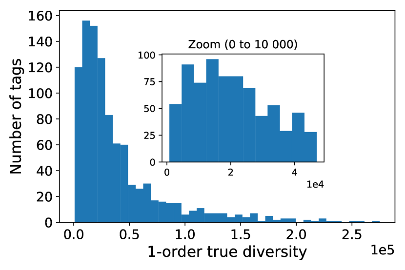
(a) ms dataset

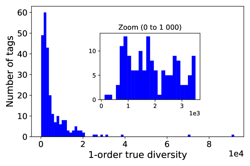
(b) amazon dataset

Figure 9: Histograms showing the distributions of the 1-order true diversities of the tag audience ($D_{1}(p_{\Pi_{\text{audience}}|t})$ for all tags in $V_{\text{tags}}$) for the ms (left) and the amazon (right) datasets.

Both plots show strongly heterogeneous distributions of individual diversities: if most of the tags have a rather narrow audience, one can identify some tags with a particularly high diversity. This is the case for the tags Rock and Pop in both datasets (see Figure 10). But even for those tags, their diversity value (around $10^{5}$ in ms and $10^{4}$ in amazon) is still one order of magnitude lower than the maximal theoretical values: 1,019,190 for ms and 465,249 for amazon (cf. Axiom 4). One can, however, nuance this observation by noticing that small diversity values are more homogeneously distributed. This is visible in the insets of Figure 9, which focus on the distribution of diversity values that are lower than 10,000 ($74\%$ of the nodes in ms, Figure 9(a)) and lower than 1,000 ($56\%$ of the nodes in amazon, Figure 9(b)). One can see in particular that the values are well distributed around the mean value of the dataset (respectively 24,850 for ms and and 2,905 for amazon). This indicates that while one may spot some extremely diverse musical contents (Rock and Pop, for instance), most of them are narrowed towards a smaller and less diverse set of users (such as Country and Punkrock in ms or New-Age in amazon).

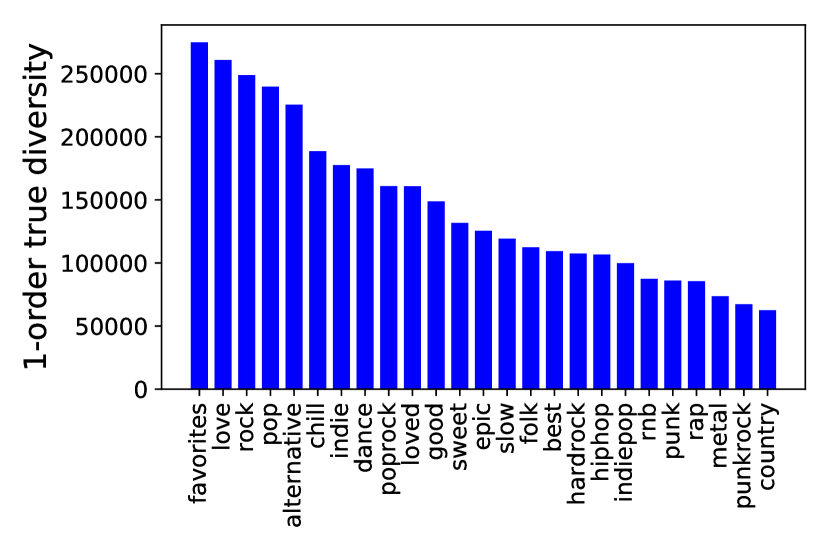
(a) ms dataset

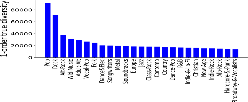
(b) amazon dataset

Figure 10: Ordered 1-order true diversities of the tag audience $D_{1}(p_{\Pi_{\text{audience}}|t})$ for 25 selected tags for the ms (left) and the amazon (right) datasets.

In order to further investigate how such diversity measures can be used to analyze specific categories, we show in Figure 10 a selection of 25 tags for the two datasets. It is worth mentioning here that for the ms dataset, the tags are actually provided by the users themselves that can decide to use any word to tag any song (this is known as a folksonomy [113]). While most tags coincide with common music genres (like Rock, Pop, Folk, Metal, …), others are obviously meant to give an appreciation of the songs (like Favorites, Love, Best, …) or even to depict a moment at which a song is listened to (like BeforeSleep or InShower). The wide range of usage of the tags is an opportunity for us to assess how our network diversity measures respond to those different behaviors. For instance, one can expect tags like Favorites to be related to a broader and more diverse audience than Metal since the songs tagged by the former do not belong to a dedicated musical category. This is indeed confirmed by Figure 10(a) which shows that popular tags like Favorites and Love have a diversity higher than any other tags of the dataset.

In contrast with the case of the ms dataset, the classification imposed by Amazon provides only tags that describe musical genres. This allows for a direct comparison of the musical categories presented in Figure 10(b), which provides interesting insights on the way users commit to the different categories. For instance, if we compare Adult-Alternative and World-Music with R&B and Dance-Pop, it is remarkable that the two former ones have a diversity twice higher although the four tags have songs reviewed by the same number of users (approximately 300,000 users). This is a clear indication that users posting reviews on Adult-Alternative and World-Music songs are much more committed (the reviews are more uniformly distributed among the users) than the ones of R&B and Dance-Pop.

5.2.3 1-order true diversity of users’ attention.

We now turn to the diversity of users’ attention, the diversity of tags listened by users. Figure 11 presents the distribution of the 1-order true diversities $D_{1}(p_{\Pi_{\text{audience}}|t})$ for all users $u\in V_{\text{users}}$. We compute and present these values using the ms (Figure 11(a)) and amazon (Figure 11(b)) datasets. In contrast with the distributions presented in Figure 9, the diversity of users’ attention is clearly homogeneous and centered around small values (compared to the maximal theoretical ones). This indicates that even if some users have a particularly high diversity, the vast majority of them have a relatively narrow consumption of the musical products. It is worth noting that, compared to the study of tags, that often had a meaningful name, we have no information regarding the profile of a user who is just an anonymized value in the dataset. Thus we cannot focus on specific users to provide an interpretation of the diversity values like we did in the previous section.

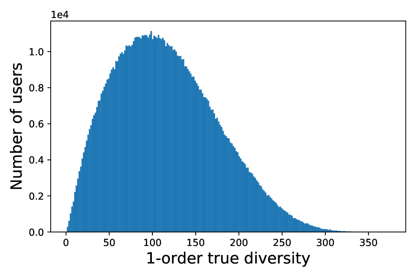
(a) ms dataset

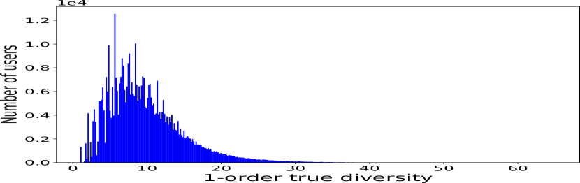
(b) amazon dataset

Figure 11: Histograms showing the distributions of the 1-order true diversities of the attention of users ($D_{1}(p_{\Pi_{\text{attention}}|u})$) for users $u\in V_{\text{users}}$ for the ms (left) and amazon (right) datasets.

However, it is possible to study how the diversity of the users depends on their activity on the platform. More precisely, let us define the volume of a user $u\in V_{\text{users}}$ as the sum of the number of tags for all songs listened to (in the case of the ms dataset) or reviewed (in the case of the amazon dataset) by $u$, multiplied by their play count (the number of songs consumed by user $u$). Then we can investigate whether there is a correlation between volume and diversity. Intuitively, the highest the volume, the highest the diversity: as its volume increases, a user has indeed more opportunities to explores new musical categories, thus diversifying its activity on the platform.

To see this more clearly, Figure 12 presents the mean value of the 1-order true diversity of a user as a function of its volume, along with the $5^{th}$-, $30^{th}$-, $70^{th}$- and $95^{th}$-percentile. For both dataset, we can observe that the diversity increases along with the volume. However, we can also notice that the influence of the volume is clearly lower after a given threshold, highlighting a saturation process in the diversity of users’ attention: while the growth of the diversity is initially sharp as the volume increases, after a given threshold (around $250$ in ms and $25$ in amazon), the users listen repeatedly to, or review similar contents proposed by the platform. This is particularly obvious in amazon (Figure 12(b)) but one can also spot this phenomenon on ms (Figure 12(a)).

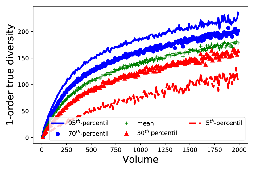
(a) ms dataset

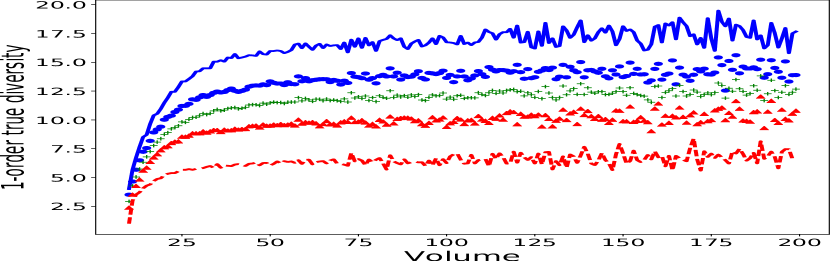
(b) amazon dataset

Figure 12: Evolution of the 1-order true diversity of users’ attention as a function of its volume for the Million Song Dataset (left) and Amazon Dataset (right).

After having presented a simple example of application of the network diversity measures in Section 5.1 and a numerical example with real datasets in this Section 5.2, we present, in the rest of Section 5 application examples for different research domains

5.3 Recommender Systems

Diversity and diversification of algorithmic recommendations has become one of the leading topics of the recommender systems research community [114, 115]. Through a variety of means, users have access today to large numbers of items (e.g., products and services in e-commerce, messages and posts in social media, or news articles in aggregators). While users enjoy an ever-growing offer, it can also become unmanageable for them to consider enough items, or to effectively explore all that is offered. Recommender systems, developed as early as in the 1980s [116], help solve this problem by filtering all possible items down to a recommended set tailored for each user or group. One recent advance in this field is the recognition of the importance of diversity and its introduction in recommendations [117, 118].

In recommender systems, diversity can help improve users’ appreciation of the quality of recommendations [119, 120]. It also has other applications, such as detecting changes in consumption behavior for context-aware recommenders [121]. As a property of recommendations, diversity has been traditionally captured by a set of related indicators proposed on intuitive bases, called serendipity, discovery, novelty, dissimilarity (see Section 8.3 of [122], or [119, 120] for a discussion of terminology and definitions). These indicators are often computed using past collective choices of items made by users [115], or classifications of items into types [20]. To this date, no general framework exists to account for all proposed diversity indices in recommender systems, nor alternatives for exploiting richer meta-data structures such as those encodable by heterogeneous information networks. This is where our proposed network diversity measures find valuable applications. They accommodate some of the existing concepts from the literature, extend the measurement of diversity to more complex data structures that can include meta-data on users and items, and give formal explicit expressions to computable quantities related to new and existing research questions in this field.

For illustrative purposes, let us consider a heterogeneous information network giving an ontology to complex data related to a situation in which we have recommended different types of items to users. Figure 13 shows the network schema of the heterogeneous information network to be considered in this example. Let us consider the following vertex types for the example:

• A vertex type of users $V_{{U}}$;

• Two vertex types for items: $V_{{I_{1}}}$ (e.g., films) and $V_{{I_{2}}}$ (e.g., series);

• Two vertex types for item classification: $V_{{T_{1}}}$ (e.g. channels/distributors) and $V_{{T_{2}}}$ (e.g. genre);

• Two vertex types of user groups: $V_{{G_{1}}}$ (e.g., demographic group) and $V_{{G_{2}}}$ (e.g., location).

Figure 13: Network schema of a heterogeneous information network in a setting from recommender systems, where users in $V_{{U}}$, belonging to groups $V_{{G_{1}}}$ and $V_{{G_{2}}}$ interact and are recommended two different sets of items $V_{{I_{1}}}$ and $V_{{I_{2}}}$, which are classified using types in $V_{{T_{1}}}$ and $V_{{T_{2}}}$.

In order to consider random walks constrained to meta paths, and following the example in Section 5.1, we denote with capital letter $X$ the random variables supported by a vertex type. For example, $X_{{U}}$ is a random vertex in $V_{{U}}$ and $X_{{I_{1}}}$ is a random vertex in $V_{{I_{1}}}$.

In the heterogeneous information network illustrated in Figure 13, we also consider different edge types:

• An edge type between users $E_{U}$ (e.g., users following or friending each others on a social network);

• Edge types from groups to users: $E_{G_{1}}$ (e.g., associating users with demographic groups) and $E_{G_{2}}$ (e.g., associating users with locations);

• Edge types indicating classification of items into types: $E_{\tau_{11}}$ and $E_{\tau_{12}}$ for $V_{{I_{1}}}$, and $E_{\tau_{22}}$ for $V_{{I_{2}}}$;

• Edge types representing when users have liked ($E_{\text{like}}$), seen ($E_{\text{seen}}$), or rated ($E_{\text{rate}}$) an item, or representing when users have been recommended items ($E_{\text{rec},1}$ and $E_{\text{rec},2}$).

All elements in the proposed example are useful for representing common practices in recommender systems. Settings for recommendation where there are two –or more– types of items ($V_{{I_{1}}}$ and $V_{{I_{2}}}$ in our example) are common in cross-domain recommendation [123], and more generally in heterogeneous information network recommendation [26]. Relations between users and items can be of different kinds in recommendation settings: edges can be used to indicate that a user has rated an item in explicit feedback –or scoring, or noting– systems ($E_{\text{rate}}$ in the example), or to indicate that a user has liked an item in implicit feedback systems ($E_{\text{like}}$ in the example). Some recommender systems and diversity measures can take into account whether a user has previously seen an item [124] ($E_{\text{seen}}$ in the example). Also, settings where meta-data are associated with users is very common in demographic or location filtering [125], and are represented in the example by using vertex types $V_{{G_{1}}}$ and $V_{{G_{2}}}$. Finally, edges between users signaling relations such as friendship of a user following another one on social networks ($E_{U}$ in the example) may also be exploited for recommendations [126, 127], and certainly in diversity computations. As stated before, Figure 13 represents the network schema (cf. Definition 7) of our example.

Most diversity computations in recommender systems consist in providing a measure of the diversity of items recommended to a user, or an aggregation of this quantity for all users. Diversity between items can be computed, for example, with respect to a classification of items [20] (e.g., genres for films). In the proposed framework, this concept would be captured by the individual diversity. Let us imagine that $V_{{U}}$ are users, that $V_{{I_{2}}}$ are films, and that $V_{{T_{2}}}$ are film genres (e.g., comedy, thriller, etc.). The individual genre ($V_{{T_{2}}}$) diversity of films ($V_{{I_{2}}}$) recommended to a user $u\in V_{{U}}$ is

$$D_{\alpha}\left(X_{{U}}\xrightarrow{E_{\text{rec},2}}X_{{I_{2}}}\xrightarrow{E_{\tau_{12}}}X_{{T_{1}}}\>|\>X_{{U}}=u\right).$$

Similarly, the mean genre ($V_{{T_{2}}}$) diversity of films ($V_{{I_{2}}}$) recommended to all users $V_{{U}}$ is the mean individual diversity

$$D_{\alpha}\left(X_{{U}}\xrightarrow{E_{\text{rec},2}}X_{{I_{2}}}\xrightarrow{E_{\tau_{12}}}X_{{T_{1}}}\>|\>X_{{U}}\right),$$

which can be computed as a geometric mean by choosing $X_{{U}}\sim\text{Uniform}(V_{{U}})$ for the starting point of the meta path constrained random walk.

In another classic setting, the diversity of an item is computed according to the number of users that have previously chosen or liked it (sometimes called novelty [128]). In the proposed framework, an aggregation of this quantity for items proposed to all users corresponds to the following network diversity measure:

$$D_{\alpha}\left(X_{{U}}\xrightarrow{E_{\text{rec},1}}X_{{I_{1}}}\xrightarrow{E_{\text{like}}^{\intercal}}X_{{U}}^{\prime}\>|\>X_{{U}}\right).$$

More interestingly, other relevant quantities expressible as network diversity measures have no explicit expression in other frameworks of the literature. The clearest example is the comparison between the mean individual and collective recommended diversities: for example, $D_{\alpha}\left(X_{{U}}\xrightarrow{E_{\text{rec},1}}X_{{I_{1}}}\xrightarrow{E_{\tau_{11}}}X_{{T_{1}}}\>|\>X_{{U}}\right)$ versus $D_{\alpha}\left(X_{{U}}\xrightarrow{E_{\text{rec},1}}X_{{I_{1}}}\xrightarrow{E_{\tau_{11}}}X_{{T_{1}}}\right)$. Distinguishing between these two concepts (cf. Figure 6) is important when taking interest in diversity beyond its use as a quality of recommendations; for example, when studying phenomena such as filter bubbles, which could manifest at some level of aggregation of users, while still having a high collective diversity. Some concepts at the core of Recommender Systems could also be expressed in our network diversity framework, such as the so-called User-Based Collaborative Filtering (see Section 4.2 of [122]):

$$D_{\alpha}\left(X_{{U}}\xrightarrow{E_{\text{rec},1}}V_{{I_{1}}}\xrightarrow{E_{\text{like}}^{\intercal}}X_{{U}}^{\prime}\xrightarrow{E_{\text{like}}}V_{{I_{1}}}^{\prime}\xrightarrow{E_{\tau_{11}}}V_{{T_{1}}}\right),$$

which corresponds to the collective type diversity of items chosen by users that chose items recommended to users.

Let us present in a schematic fashion, in Table 3, different examples of concepts related to diversity that are of interest for research questions in the domain of recommender systems, along with the respective quantities that can be identified, expressed, and computed as network diversity measures. The reader is referred to [morales2020testing] for an example of the application of the network diversity measures in conjunction with recommendation tasks. In the cited article, after presenting different experimental protocols and datasets known to the Recommender Systems community, the authors examine the performance of recommendations using the networks diversity measures, whose theoretical development and properties are the object of this article.

Table 3: Schematic representation of examples of concepts related to diversity in recommender systems and the network diversity measures that can be used to address them in quantitative studies.

Examples of concepts expressible in research questions	Corresponding network diversity measures
Mean individual diversity of recommendation of items $V_{{I_{1}}}$ according to types $V_{{T_{1}}}$ relative to the corresponding collective diversity	$D_{\alpha}\left(X_{{U}}\xrightarrow{E_{\text{rec},1}}X_{{I_{1}}}\xrightarrow{E_{\tau_{11}}}X_{{T_{1}}}\>\|\>X_{{U}}\xrightarrow{E_{\text{rec},1}}X_{{I_{1}}}\xrightarrow{E_{\tau_{11}}}X_{{T_{1}}}\>|\>X_{{U}}\right)$
Collective diversity of recommended items $V_{{I_{1}}}$ according types $V_{{T_{1}}}$ relative to the distribution of types of liked times	$D_{\alpha}\left(X_{{U}}\xrightarrow{E_{\text{rec},1}}X_{{I_{1}}}\xrightarrow{E_{\tau_{11}}}X_{{T_{1}}}\>\|\>X_{{U}}\xrightarrow{E_{\text{like}}}X_{{I_{1}}}\xrightarrow{E_{\tau_{11}}}X_{{T_{1}}}\right)$
Collective diversity of recommendations of items in $V_{{I_{1}}}$ (e.g., films) according to types $V_{{T_{2}}}$ (e.g., genres) relative to the one of $V_{{I_{2}}}$ (e.g., series)	$D_{\alpha}\left(X_{{U}}\xrightarrow{E_{\text{rec},1}}X_{{I_{1}}}\xrightarrow{E_{\tau_{12}}}X_{{T_{2}}}\>\|\>X_{{U}}\xrightarrow{E_{\text{rec},2}}X_{{I_{2}}}\xrightarrow{E_{\tau_{22}}}X_{{T_{2}}}\right)$
Diversity of items $V_{{I_{1}}}$ recommended to friends of $u\in V_{{U}}$ according to types $V_{{T_{1}}}$	$D_{\alpha}\left(X_{{U}}\xrightarrow{E_{U}}X_{{U}}^{\prime}\xrightarrow{E_{\text{rec},1}}X_{{I_{1}}}\xrightarrow{E_{\tau_{12}}}X_{{T_{1}}}\>|\>X_{{U}}=u\right)$
Diversity of items $V_{{I_{1}}}$ liked by group $g\in V_{{G_{1}}}$ according to types $V_{{T_{1}}}$	$D_{\alpha}\left(X_{{G_{1}}}\xrightarrow{E_{G_{1}}^{\intercal}}X_{{U}}\xrightarrow{E_{\text{like}}}X_{{I_{1}}}\xrightarrow{E_{\tau_{12}}}X_{{T_{1}}}\>|\>X_{{G_{1}}}=g\right)$
Diversity of users $V_{{U}}$ that liked items $V_{{I_{1}}}$ of type $t\in V_{{T_{2}}}$	$D_{\alpha}\left(X_{{U}}\>|\>X_{{U}}\xrightarrow{E_{\text{like}}}X_{{I_{1}}}\xrightarrow{E_{\tau_{12}}}X_{{T_{2}}}=t\right)$
Diversity of types $V_{{T_{2}}}$ chosen by user $u\in V_{{U}}$ through their choices of items in $V_{{I_{1}}}$	$D_{\alpha}\left(X_{{U}}\xrightarrow{E_{\left(E_{\text{like}},E_{\tau_{12}}\right)}}X_{{T_{2}}}\>|\>X_{{U}}=u\right)$

5.4 Social media studies, echo chambers, and filter bubbles

The study of social media has been developed into a large and ever growing wealth of results. The importance of studies about the creation, transmission, and consumption of information on social networks has become crucial. Heterogeneous information networks provide a natural formalism for the treatment of these objects, as they can accommodate a variety of entities (e.g., posts, accounts, media outlets, tags, keywords) interacting through many different relations (e.g., users publishing posts, mentioning or following other users, using tags in publication). More complex and abstract data is often analyzed in these studies, such as the political affiliations of users and media outlets [129, 130]. The analysis of phenomena such as echo chambers and filter bubbles through the measurement of diversity of information consumption is an established practice [21, 22, 131, 132, 23]. The settings of different social media studies vary. Concrete examples are the study of the Leave and Remain Brexit campaigns on Twitter [133] and the exchange of information between US Democrats and Republicans on Facebook [134].

In this section, we illustrate the use of network diversity measures for the study of information exchange on social networks. We consider, as before, a heterogeneous information network created from activity traces of social networks and media. Figure 14 shows its network schema, with which we may illustrate the use of network diversity measures in this context. In this example, we consider: users that post or share posts (or tweets, or blog entries, or comments in forums), users that can follow (or befriend) other users, posts that may mention users, include tags (e.g., hashtags), include topics (detectable, for example, by matching strings or using topic discovery methods), and even link to articles through a URL address. In many contexts, articles may be associated with media outlets, which may in turn be identified with groups or affiliations (e.g., political parties).

Figure 14: Network schema of a heterogeneous information network in a setting from social networks and media studies, suited for the study of echo chambers and filter bubbles.

The considered heterogeneous information network can accommodate different aspects considered in social media studies. For example, Gaumont et al. [129] consider relations of political affiliation of users and interactions between them, and analyze the notion of diversity of Twitter posts according to the political communities they have reached. Other studies also consider the use of entropy measures over distributions representing the proportion of users that browse given information sources [5]. Some studies, for example [135], explicitly consider networks of information items (e.g., blog posts) and the concepts that they use.

As with the example of a generic recommender systems, we present in a schematic fashion (in Table 4) different diversity-related concepts of interest for research questions in the field of social networks and media studies, along with quantities that can be computed as network diversity measures.

Table 4: Schematic representation of diversity-related concepts in social networks and media studies, and the corresponding network diversity measures that can be used to address them in quantitative studies.

Examples of concepts expressible in research questions	Corresponding network diversity measures
Collective diversity of affiliations of users	$D_{\alpha}\left(X_{\text{users}}\xrightarrow{E_{\text{identify}}}X_{\text{affiliations}}\right)$
Collective affiliation diversity of users through the contents they share	$D_{\alpha}\left(X_{\text{users}}\xrightarrow{E_{\text{share}}}X_{\text{posts}}\xrightarrow{E_{\text{link}}}X_{\text{articles}}\xrightarrow{E_{\text{belong}}}X_{\text{medias}}\xrightarrow{E_{\text{affiliate}}}X_{\text{affiliations}}\right)$
Individual topic diversity of user $u\in V_{\text{users}}$ through posting	$D_{\alpha}\left(X_{\text{users}}\xrightarrow{E_{\text{post}}}X_{\text{posts}}\xrightarrow{E_{\text{include}}}X_{\text{topics}}\>|\>X_{\text{users}}=u\right)$
Individual topic diversity of user $u\in V_{\text{users}}$ through posting of followers	$D_{\alpha}\left(X_{\text{users}}\xrightarrow{E_{\text{follow}}^{\intercal}}X_{\text{users}}^{\prime}\xrightarrow{E_{\text{post}}}X_{\text{posts}}\xrightarrow{E_{\text{include}}}X_{\text{topics}}\>|\>X_{\text{users}}=u\right)$
Individual affiliation diversity of users mentioned by user $u\in V_{\text{users}}$	$D_{\alpha}\left(X_{\text{users}}\xrightarrow{E_{\text{post}}}X_{\text{posts}}\xrightarrow{E_{\text{mention}}}X_{\text{users}}^{\prime}\xrightarrow{E_{\text{identify}}}X_{\text{affiliations}}\>|\>X_{\text{users}}=u\right)$
Diversity of affiliation groups that treat topic $t\in V_{\text{topics}}$ in articles	$D_{\alpha}\left(X_{\text{affiliations}}\>|\>X_{\text{affiliations}}\xrightarrow{E_{\text{affiliate}}^{\intercal}}X_{\text{medias}}\xrightarrow{E_{\text{belong}}^{\intercal}}X_{\text{articles}}\xrightarrow{E_{\text{treat}}}V_{\text{topics}}=t\right)$
Affiliation diversity of users according to who they mention in their posts relative to their own identified political affiliation	$D_{\alpha}\left(X_{\text{users}}\xrightarrow{E_{\text{post}}}X_{\text{posts}}\xrightarrow{E_{\text{mention}}}X_{\text{users}}^{\prime}\xrightarrow{E_{\text{identify}}}X_{\text{affiliations}}\>\|\>X_{\text{users}}\xrightarrow{E_{\text{identify}}}X_{\text{affiliations}}\right)$

5.5 Ecology

Diversity is useful in ecology, as identified and commented in Section 2.2. Many advances in diversity measures come from this community (e.g., [13]). One prominent concept in this domain is the diversity of species in a habitat. For the computation of quantitative indices of this diversity, individuals from different species are counted or their number is estimated. From their apportionment into the species present in a habitat, diversity is then computed and reported.

Interactions among organisms are also of interest in ecology. These can be treated using graph representations and models. One of such interactions, also related to diversity, is represented by so-called food webs [136]: network models that describe species that feed on other species. In the past, there have been efforts to use graph formalisms to treat food webs [137, 138]. Similarly, other relations between species have been described using graphs, such as parasitation [139]. Another subject of interest in ecology is the description of habitats and their interconnectedness; there have been several approaches using graph theory to describe these connections [140, 141].

We suggest that all these elements present in ecology can be treated using heterogeneous information networks. Using network diversity measures, different concepts related to diversity can be computed. Let us consider for example a heterogeneous information network with vertex types for habitats ($V_{\text{habitats}}$), for individuals ($V_{\text{individuals}}$), for species ($V_{\text{species}}$), for genera ($V_{\text{genera}}$), for families ($V_{\text{families}}$), and so on as needed.

Let us also consider for our example several edge types. Edge type $E_{\text{connect}}$ is that of edges between habitats, indicating whether an individual can access a given habitat from another one. Edge type $E_{\text{inhabit}}$ is used to represent which individuals inhabit which habitats. Edge types $E_{\text{eat}}$ and $E_{\text{parasite}}$ are used to represent relations between species; which species eat which species, and similarly for parasitation. Edge type $E_{\text{belong,1}}$ is used to represent which individual belongs to which species. Finally, edge types $E_{\text{belong,2}}$ and $E_{\text{belong,3}}$ contain edges indicating which specie belongs to which genus, and which genus belongs to which family (species, genera, and families are three of the eight major taxonomic ranks in biological classification).

This setting can accommodate the common practices of measurement of –bio– diversity of a habitat $h\in V_{\text{habitats}}$, which in network diversity measures finds the expression

$$D_{\alpha}\left(X_{\text{habitats}}\xrightarrow{E_{\text{inhabit}}^{\intercal}}X_{\text{individuals}}\xrightarrow{E_{\text{belong,1}}}X_{\text{species}}\>|\>X_{\text{habitats}}=h\right),$$

with $\alpha=0$ giving the richness biodiversity, and $\alpha=\infty$ the Berger-Parker biodiversity of the habitat. Figure 15 illustrates the network schema of the described heterogeneous information network, along with a table of diversity-related concepts and their expressions as network diversity measures.

Examples of concepts expressible in research questions	Corresponding network diversity measures
Species diversity in habitat $h\in V_{\text{habitats}}$	$D_{\alpha}\left(X_{\text{species}}\>|\>X_{\text{species}}\xrightarrow{E_{\text{belong,1}}^{\intercal}}X_{\text{individuals}}\xrightarrow{E_{\text{inhabit}}}X_{\text{habitats}}=h\right)$
Genera diversity in habitat $h\in V_{\text{habitats}}$	$D_{\alpha}\left(X_{\text{genera}}\>|\>X_{\text{genera}}\xrightarrow{E_{\text{belong,2}}^{\intercal}}X_{\text{species}}\xrightarrow{E_{\text{belong,1}}^{\intercal}}X_{\text{individuals}}\xrightarrow{E_{\text{inhabit}}}X_{\text{habitats}}=h\right)$
Species diversity of habitats adjacent to those where a species $s\in V_{\text{species}}$ is present	$D_{\alpha}\left(X_{\text{species}}\xrightarrow{E_{\text{belong,1}}^{\intercal}}X_{\text{individuals}}\xrightarrow{E_{\text{inhabit}}}X_{\text{habitats}}\xrightarrow{E_{\text{connect}}}X_{\text{habitats}}^{\prime}\right.$ $\left.\quad\quad\quad\quad\quad\quad\quad\quad\quad\quad\xrightarrow{E_{\text{inhabit}}^{\intercal}}X_{\text{individuals}}^{\prime}\xrightarrow{E_{\text{belong,1}}}X_{\text{species}}^{\prime}\>|\>X_{\text{species}}=s\right)$
Species diversity of the predators of species that parasite a species $s\in V_{\text{species}}$	$D_{\alpha}\left(X_{\text{species}}\>|\>X_{\text{species}}\xrightarrow{E_{\text{eat}}}X_{\text{species}}^{\prime}\xrightarrow{E_{\text{parasite}}}X_{\text{species}}^{\prime\prime}=s\right)$
Diversity in habitat $h_{1}\in V_{\text{habitats}}$ relative to another habitat $h_{2}\in V_{\text{habitats}}$	$D_{\alpha}\left(X_{\text{habitats}}\xrightarrow{E_{\text{inhabit}}^{\intercal}}X_{\text{individuals}}\xrightarrow{E_{\text{belong,1}}}X_{\text{species}}\>|\>X_{\text{habitats}}=h_{1}\>\|\>\right.$ $\left.\quad\quad\quad\quad X_{\text{habitats}}^{\prime}\xrightarrow{E_{\text{inhabit}}^{\intercal}}X_{\text{individuals}}^{\prime}\xrightarrow{E_{\text{belong,1}}}X_{\text{species}}^{\prime}\>|\>X_{\text{habitats}}^{\prime}=h_{2}\right)$

Figure 15: Network schema of an example from ecology, and table with examples of diversity-related concepts and their expression as network diversity measures.

5.6 Antitrust and competition law

Many developments and applications of concentration measures are found in the economics community, antitrust regulation, and competition law. As shown in Section 2.2, concentration is a concept for which indices are the reciprocal of those used for the concept of diversity. Concentration or diversity indices are used to measure the degree to which some firms concentrate the production of units (or the provision of services) in an industry. Let us consider, for example, the classification and apportionment of tons of steel produced –in a given period of time in a given country– by the firms that produced them. From this apportionment or distribution, concentration of the steel industry can be quantitatively measured with diversity measures. This is the subject of the doctoral thesis of O. C. Herfindahl, for which he developed what is now known as the Herfindahl-Hirschman Index [67]. The quantitative measurement of concentration of an industry allows for important comparisons to be made by industry regulators, such as, for example, the degree of concentration of an industry should a given merger or acquisition be allowed.

This exercise in measurement of industrial concentration, and the detection and limitation of monopolistic behavior, is made significantly more difficult by the existence of cross-ownership, or cross-control relation between firms. Cross-ownership refers to situations in which firms from an industry are mutually owned in complex, network-like relations (in a simple example between two firms A and B, firm A owns a part of firm B, and firm B owns a part of firm A). Cross-control refers, similarly, to situations where firms can name board members of other firms in the same industry producing complex relations of control in a network-like fashion.

Specialized economics literature accounts for many case studies that challenge the application of the aforementioned procedure to regulation [142, 143], and that address the complex structure of co-ownership networks and their importance in regulation [144, 145]. This makes graph-theoretical approaches good candidates for making advances in the measurement of concentration in industries [146]. In particular, the proposed network diversity measures provide tools that allow the measurement of many concepts of interest in antitrust regulation and competition law when dealing with network structures.

To illustrate this, let us consider a heterogeneous information network with three vertex types: that of vertices representing produced units of services ${V}_{\text{units}}$ (e.g., tons of steel, barrels of oil, or clients of portable phone services), that of vertices representing firms ${V}_{\text{firms}}$ that produce those units or provide those services, and that of persons ${V}_{\text{persons}}$ that own the firms. To model the relations between these entities represented by vertex types, let us consider five edge types: $E_{\text{produced}}$, linking each units to the firm that produced them, $E_{\text{own}}$, linking firms to the persons that own them, $E_{\text{cross-own}}$, linking firms with each other according to cross-ownership, and similarly, $E_{\text{control}}$ and $E_{\text{cross-control}}$ linking firms with each other according to control and cross-control (for example, having the right to choose a member of the board of a given firm). For edge types $E_{\text{own}}$, $E_{\text{cross-own}}$, $E_{\text{control}}$, and $E_{\text{cross-control}}$, the multiplicity of edges can account for the units by which property or control is represented, such as, for example, shares or members of the boards of the firms. For example, if ownership of a firm is represented by 10 shares, it will have 10 edges, that can belong to edge types $E_{\text{own}}$ or $E_{\text{cross-own}}$.

In this setting the common measurement of industry diversity is expressed as

$$D_{\alpha}\left({X}_{\text{units}}\xrightarrow{E_{\text{produced}}}{X}_{\text{firms}}\right),$$

which becomes the Herfindahl-Hirschman Diversity (reciprocal of the Herfindahl-Hirschman Index) by choosing $\alpha=2$. Figure 16 illustrates the heterogeneous information network described in this example, along with a table of concepts related to diversity and expressible using the proposed network diversity measures.

Examples of concepts expressible in research questions	Corresponding network diversity measures
Industry diversity with cross-ownership relations	$D_{\alpha}\left({X}_{\text{units}}\xrightarrow{E_{\text{produced}}}{X}_{\text{firms}}\xrightarrow{E_{\text{cross-own}}}{X}_{\text{firms}}^{\prime}\right)$
Industry diversity according to persons with cross-ownership relations	$D_{\alpha}\left({X}_{\text{units}}\xrightarrow{E_{\text{produced}}}{X}_{\text{firms}}\xrightarrow{E_{\text{cross-own}}}{X}_{\text{firms}}^{\prime}\xrightarrow{E_{\text{own}}}{X}_{\text{persons}}\right)$
Diversity of cross-ownership of a firm $f\in{V}_{\text{firms}}$	$D_{\alpha}\left({X}_{\text{firms}}\xrightarrow{E_{\text{cross-own}}}{X}_{\text{firms}}^{\prime}\>|\>{X}_{\text{firms}}=f\right)$
Diversity of ownership of firms relative to their diversity of control	$D_{\alpha}\left({X}_{\text{firms}}\xrightarrow{E_{\text{own}}}{X}_{\text{persons}}\>\|\>{X}_{\text{firms}}^{\prime}\xrightarrow{E_{\text{control}}}{X}_{\text{persons}}^{\prime}\right)$

Figure 16: Network schema of a cross-ownership and cross-control heterogeneous information network in a setting from antitrust regulation or competition law, where products are apportioned in the firms that produced them, which can be cross-owned or cross-controlled by each others.

5.7 Scientometrics

Scientometrics, within the field of bibliometrics, studies the measurement and analysis of scientific literature. Overlapping with information systems, scientometrics study, for example, the importance of publications in networks of citations using metrics such as the Impact Factor or the Science Citation Index. In networks including other entities such as authors, other measurements include the h-index, an index for the productivity and citation impact of scholars. Recent studies have used heterogeneous information networks to represent data including other entities, such as journals and conferences, in order to extract extended measurements [147].

The study of networks modeling and representing scientific production is of interest for other reasons too. Diversity of topics explored by scientific communities is a concept of interest, for example, in public policy [148], and in general for the understanding and description of the structure of scientific communities [149, 150]. Another practical application of the measurement of diversity in citation networks is the maintenance of classification systems [151].

Below, we illustrate the way proposed network diversity measures can address some of the concepts relevant to these areas of research by means of an example. Let us consider a heterogeneous information network consisting of the following vertex types: authors ${V}_{\text{authors}}$, laboratories ${V}_{\text{lab.}}$ (or affiliation institutions), journals ${V}_{\text{journals}}$, scientific articles ${V}_{\text{papers}}$, keywords used by these articles ${V}_{\text{keywords}}$, and domains of research ${V}_{\text{domains}}$ (e.g., ecology, economics). We also consider edge types for representing relations between these entities (see Figure 17): affiliation $E_{\text{aff.}}$ of authors to institutions, edition (or peer-review) $E_{\text{edit}}$ of journals by authors, writing $E_{\text{write}}$ of articles by authors, use of keywords $E_{\text{use}}$ in articles, association of keywords $E_{\text{belong}}$ with domains, publication $E_{\text{publish}}$ of articles by journals, and declared treatment $E_{\text{treat}}$ of research domains by journals. Figure 17 illustrates the corresponding heterogeneous information network, along with a table of concepts related to diversity and expressible using the proposed network diversity measures.

Examples of concepts expressible in research questions	Corresponding network diversity measures
Diversity of keywords used by author $a\in{V}_{\text{authors}}$	$D_{\alpha}\left({X}_{\text{authors}}\xrightarrow{E_{\text{write}}}{X}_{\text{papers}}\xrightarrow{E_{\text{use}}}{X}_{\text{keywords}}\>|\>{X}_{\text{authors}}=a\right)$
Diversity of domains addressed in publications by author $a\in{V}_{\text{authors}}$ relative to domains he or she addresses in editing (or peer-reviewing)	$D_{\alpha}\left({X}_{\text{authors}}\xrightarrow{E_{\text{write}}}{X}_{\text{papers}}\xrightarrow{E_{\text{use}}}{X}_{\text{keywords}}\xrightarrow{E_{\text{belong}}}{X}_{\text{domains}}\>|\>{X}_{\text{authors}}=a\>\|\>\right.$
	$\quad\quad\quad\quad\left.{X}_{\text{authors}}^{\prime}\xrightarrow{E_{\text{edit}}}{X}_{\text{journals}}\xrightarrow{E_{\text{treat}}}{X}_{\text{domains}}^{\prime}\>|\>{X}_{\text{authors}}^{\prime}=a\right)$
Diversity of domains addressed by citations by authors of laboratory $l\in{V}_{\text{lab.}}$	$D_{\alpha}\left({X}_{\text{lab.}}\xrightarrow{E_{\text{aff.}}^{\intercal}}{X}_{\text{authors}}\xrightarrow{E_{\text{write}}}{X}_{\text{papers}}\xrightarrow{E_{\text{cite}}}{X}_{\text{papers}}^{\prime}\xrightarrow{E_{\text{use}}}{X}_{\text{keywords}}\xrightarrow{E_{\text{belong}}}{X}_{\text{domains}}\>|\>{X}_{\text{lab.}}=l\right)$

Figure 17: Network schema of a heterogeneous information network in an example for scientometrics, and table of examples of concepts related to diversity and expressible using the proposed network diversity measures.

6 Conclusions

This article presents a formal framework for the measurement of diversity in heterogeneous information networks. This allows for the extension of the application of diversity measures from classification modeled by apportioning into distributions, to data represented in network structures.

By presenting a concise theory resulting from the imposition of desirable properties of axioms, we organize diversity measures across a wide spectrum of domains into a family of functions defined by a single parameter $\alpha$: the true diversities. Providing a formalism for heterogeneous information networks and constrained random walks on it, we consider different probability distributions on which diversity measures are computed. These diversity measures are related to the structure of the heterogeneous information network, and thus to the phenomena or objects it represents. Diversity measures are also related to the different ways in which distributions are computed, which allows us to distinguish several types of diversities: collective, individual, mean individual, backward, relative, and projected diversities. Some of these network diversities relate to existing measures in the literature, that we framed into a comprehensive framework. But they also allow for the treatment of new concepts related to diversity in networks. We provide examples of applications in several domains.

The main contributions of this article are:

• The proposition of an axiomatic theory of diversity measures that allows us to present most of their uses across several domains with a single-parameter family of functions.

• The formalization of concepts and tools to describe and process heterogeneous information networks, that have been gaining attention in representation learning and information retrieval communities (in particular in recommender systems).

• The definition of several network diversity measures, resulting from the application of true diversities to probability distributions that are computable with the heterogeneous information network formalism. These network diversity measures allow for the referentiation, expression, and computation of concepts relevant to diversity in networks, extending the use of diversity from systems of classification and apportionment to systems best described by network-structured data.

• The mapping of some of the network diversity measures to pre-existing quantitative measurements that are widespread in different fields, and the development of new applications through examples in recommender systems, social media studies, ecology, competition law, and scientometrics.

In addition to providing means of referencing, expression, and computation on diversity-related concepts in complex data modeled by heterogeneous information networks, the network diversity measures could be leveraged in different downstream tasks performed in data mining. Expanding on those mentioned in the introduction (Section 1), we can now hint at more precise examples of applications in such tasks. In Recommender Systems, for example, previous works have used diversities associated with meta paths to avoid over-fitting in the training stage on data modeled with heterogeneous information networks [152]. Network diversity measures could allow, in this case, to target different collective and individual diversities in the function to be optimized. Other applications use meta paths to consider node similarities in strategies for node classification [153], and could leverage network diversity measures to consider parametrization of the weight given to balance and variety in diversity when used. Research in representation learning could embed different quantities computable with network diversity measures in learning strategies where diversity would be leveraged for optimizing different objective function through training [154]. Finally, we hint to other applications that would need to be explored in greater detail than it is possible here, in domains related to heterogeneous information networks and diversity, such as community detection [155, 156, 157], clustering in networks [158, 159], and the analysis of time-series resulting from temporal networks [160].

Many relevant advances in computer sciences hinge on the improvement of performance metrics through the development of novel algorithms and methodologies. This article seeks to contribute in the proposal of the metrics with which advacements are to be compared with the state of art. It is for this purpose what we propose a detailed discussion of the properties and implications of the proposed network diversity measures. We hope that this framework for the application of diversity measures to network structures will enrich research on diversity in the domains identified in Section 5 and beyond. Future developments in this line of research might consider the identification of algebraic structures for network diversity measures, and their application to case studies.

References

- [1] K. S. McCann, The diversity–stability debate, Nature 405 (6783) (2000) 228.
- [2] P. Geroski, et al., The choice between diversity and scale, Davis, E., Geroski, PA, Kay, J. A., Manning A., Smales, C., Smith, SR and Szymanski, S.(eds.) (1992) 29–45.
- [3] J. Aczél, Z. Daróczy, On measures of information and their characterizations, New York (1975) 168.
- [4] A. Rényi, et al., On measures of entropy and information, in: Proceedings of the Fourth Berkeley Symposium on Mathematical Statistics and Probability, Volume 1: Contributions to the Theory of Statistics, The Regents of the University of California, 1961, pp. 547–561.
- [5] D. Nikolov, D. F. Oliveira, A. Flammini, F. Menczer, Measuring online social bubbles, PeerJ Computer Science 1 (2015) e38.
- [6] J. Kulshrestha, M. B. Zafar, L. E. Noboa, K. P. Gummadi, S. Ghosh, Characterizing information diets of social media users., in: ICWSM, 2015, pp. 218–227.
- [7] R. K. Ursem, Diversity-guided evolutionary algorithms, in: International Conference on Parallel Problem Solving from Nature, Springer, 2002, pp. 462–471.
- [8] J. Riget, J. S. Vesterstrøm, A diversity-guided particle swarm optimizer-the arpso, Dept. Comput. Sci., Univ. of Aarhus, Aarhus, Denmark, Tech. Rep 2 (2002) 2002.
- [9] A. Stirling, A general framework for analysing diversity in science, technology and society, Journal of the Royal Society Interface 4 (15) (2007) 707–719.
- [10] C. E. Shannon, A mathematical theory of communication, Bell system technical journal 27 (3) (1948) 379–423.
- [11] C. Gini, Measurement of inequality of incomes, The Economic Journal 31 (121) (1921) 124–126.
- [12] S. A. Rhoades, The herfindahl-hirschman index, Fed. Res. Bull. 79 (1993) 188.
- [13] M. O. Hill, Diversity and evenness: a unifying notation and its consequences, Ecology 54 (2) (1973) 427–432.
- [14] D. Encaoua, A. Jacquemin, Degree of monopoly, indices of concentration and threat of entry, International economic review (1980) 87–105.
- [15] S. R. Chakravarty, W. Eichhorn, An axiomatic characterization of a generalized index of concentration, Journal of Productivity Analysis 2 (2) (1991) 103–112.
- [16] F. Pasquale, The Black Box Society: The Secret Algorithms That Control Money and Information, Harvard University Press, Cambridge, MA, USA, 2015.
- [17] E. Pariser, The Filter Bubble: What The Internet Is Hiding From You, Penguin Books Limited, 2011.
- [18] A. Datta, J. Makagon, D. Mulligan, M. Tschantz, Discrimination in online personalization: A multidisciplinary inquiry, in: Proceedings of the 1st Conference on Fairness, Accountability and Transparency, ACM, 2018.
- [19] R. Courtland, Bias detectives: the researchers striving to make algorithms fair, Nature 558 (7710) (2018) 357–360.
- [20] C.-N. Ziegler, S. M. McNee, J. A. Konstan, G. Lausen, Improving recommendation lists through topic diversification, in: Proceedings of the 14th international conference on World Wide Web, ACM, 2005, pp. 22–32.
- [21] B. Smyth, P. McClave, Similarity vs. diversity, in: Proceedings of the 4th International Conference on Case-Based Reasoning: Case-Based Reasoning Research and Development, ICCBR ’01, Springer-Verlag, 2001, pp. 347–361.
- [22] A.-A. Stoica, C. Riederer, A. Chaintreau, Algorithmic glass ceiling in social networks: The effects of social recommendations on network diversity, in: Proceedings of the 2018 World Wide Web Conference, ACM, 2018, pp. 923–932.
- [23] M. Schedl, P. Knees, F. Gouyon, New paths in music recommender systems research, in: Proceedings of the Eleventh ACM Conference on Recommender Systems, ACM, 2017, pp. 392–393.
- [24] Y. Sun, J. Han, Mining heterogeneous information networks: a structural analysis approach, Acm Sigkdd Explorations Newsletter 14 (2) (2013) 20–28.
- [25] Y. Sun, Y. Yu, J. Han, Ranking-based clustering of heterogeneous information networks with star network schema, in: Proceedings of the 15th ACM SIGKDD international conference on Knowledge discovery and data mining, ACM, 2009, pp. 797–806.
- [26] X. Yu, X. Ren, Y. Sun, Q. Gu, B. Sturt, U. Khandelwal, B. Norick, J. Han, Personalized entity recommendation: A heterogeneous information network approach, in: Proceedings of the 7th ACM international conference on Web search and data mining, ACM, 2014, pp. 283–292.
- [27] T.-y. Fu, W.-C. Lee, Z. Lei, Hin2vec: Explore meta-paths in heterogeneous information networks for representation learning, in: Proceedings of the 2017 ACM on Conference on Information and Knowledge Management, ACM, 2017, pp. 1797–1806.
- [28] M. Sydow, M. Pikuła, R. Schenkel, The notion of diversity in graphical entity summarisation on semantic knowledge graphs, Journal of Intelligent Information Systems 41 (2) (2013) 109–149.
- [29] Y. Chen, C. Wang, Hine: heterogeneous information network embedding, in: International Conference on Database Systems for Advanced Applications, Springer, 2017, pp. 180–195.
- [30] M. De Domenico, A. Solé-Ribalta, E. Cozzo, M. Kivelä, Y. Moreno, M. A. Porter, S. Gómez, A. Arenas, Mathematical formulation of multilayer networks, Physical Review X 3 (4) (2013) 041022.
- [31] M. De Domenico, A. Solé-Ribalta, E. Omodei, S. Gómez, A. Arenas, Ranking in interconnected multilayer networks reveals versatile nodes, Nature communications 6 (2015) 6868.
- [32] Y. Sun, J. Han, X. Yan, P. S. Yu, T. Wu, Pathsim: Meta path-based top-k similarity search in heterogeneous information networks, Proceedings of the VLDB Endowment 4 (11) (2011) 992–1003.
- [33] N. Lao, W. W. Cohen, Relational retrieval using a combination of path-constrained random walks, Machine learning 81 (1) (2010) 53–67.
- [34] Y. Xiong, Y. Zhu, S. Y. Philip, Top-k similarity join in heterogeneous information networks, IEEE Transactions on Knowledge and Data Engineering 27 (6) (2014) 1710–1723.
- [35] X. Yu, X. Ren, Y. Sun, B. Sturt, U. Khandelwal, Q. Gu, B. Norick, J. Han, Recommendation in heterogeneous information networks with implicit user feedback, in: Proceedings of the 7th ACM conference on Recommender systems, ACM, 2013, pp. 347–350.
- [36] C. Shi, B. Hu, W. X. Zhao, S. Y. Philip, Heterogeneous information network embedding for recommendation, IEEE Transactions on Knowledge and Data Engineering 31 (2) (2018) 357–370.
- [37] K. Yu, S. Yu, V. Tresp, Soft clustering on graphs, in: Advances in neural information processing systems, 2006, pp. 1553–1560.
- [38] R.-H. Li, J. X. Yu, Scalable diversified ranking on large graphs, IEEE Transactions on Knowledge and Data Engineering 25 (9) (2012) 2133–2146.
- [39] D. Hristova, M. J. Williams, M. Musolesi, P. Panzarasa, C. Mascolo, Measuring urban social diversity using interconnected geo-social networks, in: Proceedings of the 25th international conference on world wide web, International World Wide Web Conferences Steering Committee, 2016, pp. 21–30.
- [40] B. King, R. Jha, D. R. Radev, Heterogeneous networks and their applications: Scientometrics, name disambiguation, and topic modeling, Transactions of the Association for Computational Linguistics 2 (2014) 1–14.
- [41] S. Nandanwar, A. Moroney, M. N. Murty, Fusing diversity in recommendations in heterogeneous information networks, in: Proceedings of the Eleventh ACM International Conference on Web Search and Data Mining, ACM, 2018, pp. 414–422.
- [42] F. Vahedian, R. Burke, B. Mobasher, Meta-path selection for extended multi-relational matrix factorization, in: The Twenty-Ninth International Flairs Conference, 2016.
- [43] X. Yu, Y. Sun, B. Norick, T. Mao, J. Han, User guided entity similarity search using meta-path selection in heterogeneous information networks, in: Proceedings of the 21st ACM international conference on Information and knowledge management, Acm, 2012, pp. 2025–2029.
- [44] G. Helfman, B. B. Collette, D. E. Facey, B. W. Bowen, The diversity of fishes: biology, evolution, and ecology, John Wiley & Sons, 2009.
- [45] S. J. McNaughton, Diversity and stability of ecological communities: a comment on the role of empiricism in ecology, The American Naturalist 111 (979) (1977) 515–525.
- [46] R. M. May, Patterns of species abundance and diversity, Ecology and evolution of communities (1975) 81–120.
- [47] J. M. Smith, Trees, bundles or nets?, Trends in ecology & evolution 4 (10) (1989) 302–304.
- [48] S. Gillett, In praise of policy diversity, position paper for oii broadband forum (2003).
- [49] G. Silverberg, G. Dosi, L. Orsenigo, Innovation, diversity and diffusion: A self-organisation model, The Economic Journal 98 (393) (1988) 1032–1054.
- [50] H. Nowotny, P. Scott, M. Gibbons, P. B. Scott, Re-thinking science: Knowledge and the public in an age of uncertainty, Cambridge: Polity Press, 200.
- [51] E. V. Shevchenko, D. V. Talapin, N. A. Kotov, S. O’brien, C. B. Murray, Structural diversity in binary nanoparticle superlattices, Nature 439 (7072) (2006) 55.
- [52] E. D. Schneider, J. J. Kay, Life as a manifestation of the second law of thermodynamics, Mathematical and computer modelling 19 (6-8) (1994) 25–48.
- [53] G. Grabher, D. Stark, Organizing diversity: evolutionary theory, network analysis and postsocialism, Regional studies 31 (5) (1997) 533–544.
- [54] W. R. Ashby, Requisite variety and its implications for the control of complex systems, in: Facets of systems science, Springer, 1991, pp. 405–417.
- [55] F. J. Dyson, Statistical theory of the energy levels of complex systems. i, Journal of Mathematical Physics 3 (1) (1962) 140–156.
- [56] H.-X. Yang, Z.-X. Wu, C. Zhou, T. Zhou, B.-H. Wang, Effects of social diversity on the emergence of global consensus in opinion dynamics, Physical Review E 80 (4) (2009) 046108.
- [57] A. Stirling, On the economics and analysis of diversity, Science Policy Research Unit (SPRU), Electronic Working Papers Series, Paper 28 (1998) 1–156.
- [58] R. H. MacArthur, Patterns of species diversity, Biological reviews 40 (4) (1965) 510–533.
- [59] N. J. Gotelli, R. K. Colwell, Estimating species richness, Biological diversity: frontiers in measurement and assessment 12 (2011) 39–54.
- [60] E. P. Odum, Fundamentals of ecology, WB Saunders company, 1959.
- [61] C. E. Shannon, W. Weaver, The mathematical theory of communication. 1949, Urbana, IL: University of Illinois Press (1963).
- [62] E. C. Pielou, et al., An introduction to mathematical ecology., An introduction to mathematical ecology. (1969).
- [63] M. Wulfmeier, P. Ondruska, I. Posner, Maximum entropy deep inverse reinforcement learning, arXiv preprint arXiv:1507.04888 (2015).
- [64] W. Wang, G. Zhang, J. Lu, Collaborative filtering with entropy-driven user similarity in recommender systems, International Journal of Intelligent Systems 30 (8) (2015) 854–870.
- [65] E. H. Simpson, Measurement of diversity., nature (1949).
- [66] A. O. Hirschman, National power and the structure of foreign trade, University of California Press, 1945.
- [67] O. C. Herfindahl, Concentration in the us steel industry, Unpublished PhD. Dissertation, Columbia University (1950).
- [68] J. P. Gibbs, W. T. Martin, Urbanization, technology, and the division of labor: International patterns, American sociological review (1962) 667–677.
- [69] M. Nei, Estimation of average heterozygosity and genetic distance from a small number of individuals, Genetics 89 (3) (1978) 583–590.
- [70] S. H. Hurlbert, The nonconcept of species diversity: a critique and alternative parameters, Ecology 52 (4) (1971) 577–586.
- [71] A. Sen, M. A. Sen, S. Amartya, J. E. Foster, J. E. Foster, et al., On economic inequality, Oxford University Press, 1997.
- [72] W. H. Berger, F. L. Parker, Diversity of planktonic foraminifera in deep-sea sediments, Science 168 (3937) (1970) 1345–1347.
- [73] M. L. Weitzman, On diversity, The Quarterly Journal of Economics 107 (2) (1992) 363–405.
- [74] A. R. Solow, S. Polasky, Measuring biological diversity, Environmental and Ecological Statistics 1 (2) (1994) 95–103.
- [75] P. H. Williams, C. Humphries, R. Vane-Wright, Measuring biodiversity: taxonomic relatedness for conservation priorities, Australian systematic botany 4 (4) (1991) 665–679.
- [76] P. Nguyen, P.-P. Saviotti, M. Trommetter, B. Bourgeois, Variety and the evolution of refinery processing, Industrial and corporate change 14 (3) (2005) 469–500.
- [77] B. Runnegar, K. Campbell, M. Day, Rates and modes of evolution in the mollusca, Rates of evolution. Allen and Unwin, London (1987) 39–60.
- [78] K. Junge, Diversity of ideas about diversity measurement, Scandinavian Journal of Psychology 35 (1) (1994) 16–26.
- [79] C. R. Rao, Rao’s axiomatization of diversity measures, Wiley StatsRef: Statistics Reference Online (2014).
- [80] I. Csiszár, Axiomatic characterizations of information measures, Entropy 10 (3) (2008) 261–273.
- [81] G. Wang, M. Jiang, Axiomatic characterization of nonlinear homomorphic means, Journal of Mathematical Analysis and Applications 303 (1) (2005) 350–363.
- [82] J. Aczél, C. Alsina, Synthesizing judgements: A functional equations approach, Mathematical Modelling 9 (3-5) (1987) 311–320.
- [83] H. Dalton, The measurement of the inequality of incomes, The Economic Journal 30 (119) (1920) 348–361.
- [84] S. Hoffmann, Concavity and additivity in diversity measurement: re-discovery of an unknown concept, Univ., FEMM, 2006.
- [85] A. N. Kolmogorov, G. Castelnuovo, Sur la notion de la moyenne, G. Bardi, tip. della R. Accad. dei Lincei, 1930.
- [86] M. Nagumo, Über eine klasse der mittelwerte, in: Japanese journal of mathematics: transactions and abstracts, Vol. 7, The Mathematical Society of Japan, 1930, pp. 71–79.
- [87] H. P. Pursiainen, Consistency in aggregation, quasilinear means and index numbers, Quasilinear Means and Index Numbers (December 4, 2008) (2008).
- [88] M. Hall, N. Tideman, Measures of concentration, Journal of the american statistical association 62 (317) (1967) 162–168.
- [89] L. Jost, Entropy and diversity, Oikos 113 (2) (2006) 363–375.
- [90] L. Hannah, J. A. Kay, Concentration in modern industry: Theory, measurement and the UK experience, Springer, 1977.
- [91] L. Jost, P. DeVries, T. Walla, H. Greeney, A. Chao, C. Ricotta, Partitioning diversity for conservation analyses, Diversity and Distributions 16 (1) (2010) 65–76.
- [92] A. J. Daly, J. M. Baetens, B. De Baets, Ecological diversity: measuring the unmeasurable, Mathematics 6 (7) (2018) 119.
- [93] P. Ramaciotti Morales, L. Tabourier, S. Ung, C. Prieur, Role of the website structure in the diversity of browsing behaviors, in: Proceedings of the 30th ACM Conference on Hypertext and Social Media, ACM, 2019, pp. 133–142.
- [94] T. Van Erven, P. Harremos, Rényi divergence and kullback-leibler divergence, IEEE Transactions on Information Theory 60 (7) (2014) 3797–3820.
- [95] S. Kullback, R. A. Leibler, On Information and Sufficiency, The Annals of Mathematical Statistics 22 (1) (1951) 79–86.
- [96] T. M. Cover, J. A. Thomas, Elements of Information Theory, Wiley Series in Telecommunications and Signal Processing, Wiley-Interscience, New York, NY, USA, 2006.
- [97] K. Bollacker, C. Evans, P. Paritosh, T. Sturge, J. Taylor, Freebase: a collaboratively created graph database for structuring human knowledge, in: Proceedings of the 2008 ACM SIGMOD international conference on Management of data, AcM, 2008, pp. 1247–1250.
- [98] G. A. Miller, Wordnet: a lexical database for english, Communications of the ACM 38 (11) (1995) 39–41.
- [99] M. Ashburner, C. A. Ball, J. A. Blake, D. Botstein, H. Butler, J. M. Cherry, A. P. Davis, K. Dolinski, S. S. Dwight, J. T. Eppig, et al., Gene ontology: tool for the unification of biology, Nature genetics 25 (1) (2000) 25.
- [100] C. Shi, Y. Li, J. Zhang, Y. Sun, S. Y. Philip, A survey of heterogeneous information network analysis, IEEE Transactions on Knowledge and Data Engineering 29 (1) (2016) 17–37.
- [101] A. Singhal, Introducing the knowledge graph: things, not strings, Official google blog 5 (2012).
-
[102]
W. W. W. Consortium, Resource description
framework (rdf).
URL https://www.w3.org/RDF/ - [103] J. Han, J.-R. Wen, Mining frequent neighborhood patterns in a large labeled graph, in: Proceedings of the 22nd ACM international conference on Information & Knowledge Management, 2013, pp. 259–268.
- [104] M. Nickel, K. Murphy, V. Tresp, E. Gabrilovich, A review of relational machine learning for knowledge graphs, Proceedings of the IEEE 104 (1) (2015) 11–33.
- [105] Y. Zheng, C. Shi, X. Cao, X. Li, B. Wu, Entity set expansion with meta path in knowledge graph, in: Pacific-Asia conference on knowledge discovery and data mining, Springer, 2017, pp. 317–329.
- [106] X. Cao, C. Shi, Y. Zheng, J. Ding, X. Li, B. Wu, A heterogeneous information network method for entity set expansion in knowledge graph, in: Pacific-Asia Conference on Knowledge Discovery and Data Mining, Springer, 2018, pp. 288–299.
- [107] N. Lao, W. W. Cohen, Fast query execution for retrieval models based on path-constrained random walks, in: Proceedings of the 16th ACM SIGKDD international conference on Knowledge discovery and data mining, ACM, 2010, pp. 881–888.
- [108] C. Shi, S. Y. Philip, Heterogeneous information network analysis and applications, Springer, 2017.
- [109] R. Poulain, F. Tarissan, Investigating the lack of diversity in user behavior: The case of musical content on online platforms, Information Processing & Management 57 (2) (2020) 102169.
- [110] T. Bertin-Mahieux, D. P. Ellis, B. Whitman, P. Lamere, The million song dataset, in: Proceedings of the 12th International Conference on Music Information Retrieval, University of Miami, 2011, pp. 591–596.
- [111] R. He, J. McAuley, Ups and downs: Modeling the visual evolution of fashion trends with one-class collaborative filtering, in: Proceedings of the 25th International Conference on World Wide Web, ACM, 2016, pp. 507–517.
- [112] J. McAuley, C. Targett, Q. Shi, A. van den Hengel, Image-based recommendations on styles and substitutes, in: Proceedings of the 38th International ACM SIGIR Conference on Research and Development in Information Retrieval, ACM, 2015, pp. 43–52.
- [113] I. Peters, Folksonomies. Indexing and retrieval in Web 2.0, Walter de Gruyter, 2009.
- [114] M. Kunaver, T. Požrl, Diversity in recommender systems–a survey, Knowledge-Based Systems 123 (2017) 154–162.
- [115] T. Zhou, Z. Kuscsik, J.-G. Liu, M. Medo, J. R. Wakeling, Y.-C. Zhang, Solving the apparent diversity-accuracy dilemma of recommender systems, Proceedings of the National Academy of Sciences 107 (10) (2010) 4511–4515.
- [116] G. Salton, M. J. McGill, Introduction to modern information retrieval, mcgraw-hill, 1983.
- [117] S. M. McNee, J. Riedl, J. A. Konstan, Being accurate is not enough: how accuracy metrics have hurt recommender systems, in: CHI’06 extended abstracts on Human factors in computing systems, ACM, 2006, pp. 1097–1101.
- [118] K. Bradley, B. Smyth, Improving recommendation diversity, in: Proceedings of the Twelfth Irish Conference on Artificial Intelligence and Cognitive Science, Maynooth, Ireland, Citeseer, 2001, pp. 85–94.
- [119] T. Silveira, M. Zhang, X. Lin, Y. Liu, S. Ma, How good your recommender system is? a survey on evaluations in recommendation, International Journal of Machine Learning and Cybernetics 10 (5) (2019) 813–831.
- [120] J. Bobadilla, F. Ortega, A. Hernando, A. Gutiérrez, Recommender systems survey, Knowledge-based systems 46 (2013) 109–132.
- [121] A. L’Huillier, S. Castagnos, A. Boyer, Modéliser la diversité au cours du temps pour détecter le contexte dans un service de musique en ligne (2016).
- [122] P. Kantor, F. Ricci, L. Rokach, B. Shapira, Recommender systems handbook, Springer, 2010.
- [123] J. Tang, S. Wu, J. Sun, H. Su, Cross-domain collaboration recommendation, in: Proceedings of the 18th ACM SIGKDD international conference on Knowledge discovery and data mining, ACM, 2012, pp. 1285–1293.
- [124] S. Vargas, P. Castells, Rank and relevance in novelty and diversity metrics for recommender systems, in: Proceedings of the fifth ACM conference on Recommender systems, ACM, 2011, pp. 109–116.
- [125] L. Safoury, A. Salah, Exploiting user demographic attributes for solving cold-start problem in recommender system, Lecture Notes on Software Engineering 1 (3) (2013) 303–307.
- [126] G. Groh, C. Ehmig, Recommendations in taste related domains: collaborative filtering vs. social filtering, in: Proceedings of the 2007 international ACM conference on Supporting group work, ACM, 2007, pp. 127–136.
- [127] D. Bernardes, M. Diaby, R. Fournier, F. FogelmanSoulié, E. Viennet, A social formalism and survey for recommender systems, Acm Sigkdd Explorations Newsletter 16 (2) (2015) 20–37.
- [128] N. Hurley, M. Zhang, Novelty and diversity in top-n recommendation–analysis and evaluation, ACM Transactions on Internet Technology (TOIT) 10 (4) (2011) 14.
- [129] N. Gaumont, M. Panahi, D. Chavalarias, Reconstruction of the socio-semantic dynamics of political activist twitter networks—method and application to the 2017 french presidential election, PloS one 13 (9) (2018) e0201879.
- [130] S. Flaxman, S. Goel, J. M. Rao, Filter bubbles, echo chambers, and online news consumption, Public opinion quarterly 80 (S1) (2016) 298–320.
- [131] C. Sha, X. Wu, J. Niu, A framework for recommending relevant and diverse items., in: IJCAI, 2016, pp. 3868–3874.
- [132] M. D. Ekstrand, M. Tian, M. R. I. Kazi, H. Mehrpouyan, D. Kluver, Exploring author gender in book rating and recommendation, in: Proceedings of the 12th ACM Conference on Recommender Systems, 2018, pp. 242–250.
- [133] M. Bastos, D. Mercea, A. Baronchelli, The geographic embedding of online echo chambers: Evidence from the brexit campaign, PloS one 13 (11) (2018) e0206841.
- [134] E. Bakshy, S. Messing, L. A. Adamic, Exposure to ideologically diverse news and opinion on facebook, Science 348 (6239) (2015) 1130–1132.
- [135] C. Roth, Socio-semantic frameworks, Advances in Complex Systems 16 (04n05) (2013) 1350013.
- [136] R. T. Paine, Food web complexity and species diversity, The American Naturalist 100 (910) (1966) 65–75.
- [137] R. M. May, Ecology: The structure of food webs, Nature 301 (5901) (1983) 566–568.
- [138] J. R. Lundgren, Food webs, competition graphs, competition-common enemy graphs, and niche graphs, in: Applications of Combinatorics and Graph Theory to the Biological and Social Sciences, Springer, 1989, pp. 221–243.
- [139] R. Poulin, Network analysis shining light on parasite ecology and diversity, Trends in parasitology 26 (10) (2010) 492–498.
- [140] D. Urban, T. Keitt, Landscape connectivity: a graph-theoretic perspective, Ecology 82 (5) (2001) 1205–1218.
- [141] M. Wirth, G. F. Estabrook, D. J. Rogers, A graph theory model for systematic biology, with an example for the oncidiinae (orchidaceae), Systematic Zoology 15 (1) (1966) 59–69.
- [142] C. Kang, Ownership structure of samsung chaebol, Beyond the firm: Business groups in international and historical perspective, ed. T. Shiba, and M. Shimotani (1997) 31–58.
- [143] H.-J. Kim, Concentrated ownership and corporate control: Wallenberg sphere and samsung group, J. Korean L. 14 (2014) 39.
- [144] H. Compston, The network of global corporate control: implications for public policy, Business and Politics 15 (3) (2013) 357–379.
- [145] S. Vitali, J. B. Glattfelder, S. Battiston, The network of global corporate control, PloS one 6 (10) (2011) e25995.
- [146] M. Levy, Control in pyramidal structures, Corporate Governance: An International Review 17 (1) (2009) 77–89.
- [147] E. Yan, Y. Ding, C. R. Sugimoto, P-rank: An indicator measuring prestige in heterogeneous scholarly networks, Journal of the American Society for Information Science and Technology 62 (3) (2011) 467–477.
- [148] M. Zitt, E. Bassecoulard, Challenges for scientometric indicators: data demining, knowledge-flow measurements and diversity issues, Ethics in science and environmental politics 8 (1) (2008) 49–60.
- [149] M. Zitt, Facing diversity of science: A challenge for bibliometric indicators, Measurement: Interdisciplinary Research and Perspectives 3 (1) (2005) 38–49.
- [150] G. Heimeriks, M. Hörlesberger, P. Van den Besselaar, Mapping communication and collaboration in heterogeneous research networks, Scientometrics 58 (2) (2003) 391–413.
- [151] I. Gómez, M. Bordons, M. Fernandez, A. Méndez, Coping with the problem of subject classification diversity, Scientometrics 35 (2) (1996) 223–235.
- [152] H. Liu, Z. Jiang, Y. Song, T. Zhang, Z. Wu, User preference modeling based on meta paths and diversity regularization in heterogeneous information networks, Knowledge-Based Systems 181 (2019) 104784.
- [153] D. Yin, H. Gao, A flexible aggregation framework on large-scale heterogeneous information networks, Journal of Information Science 43 (2) (2017) 186–203.
- [154] C. Zhang, A. Swami, N. V. Chawla, Shne: Representation learning for semantic-associated heterogeneous networks, in: Proceedings of the Twelfth ACM International Conference on Web Search and Data Mining, 2019, pp. 690–698.
- [155] J. D. Cruz, C. Bothorel, F. Poulet, Entropy based community detection in augmented social networks, in: 2011 International Conference on computational aspects of social networks (CASoN), IEEE, 2011, pp. 163–168.
- [156] A. G. Nikolaev, R. Razib, A. Kucheriya, On efficient use of entropy centrality for social network analysis and community detection, Social Networks 40 (2015) 154–162.
- [157] K. R. Žalik, B. Žalik, Memetic algorithm using node entropy and partition entropy for community detection in networks, Information Sciences 445 (2018) 38–49.
- [158] Y.-X. Wang, F. S. Bao, An entropy-based weighted clustering algorithm and its optimization for ad hoc networks, in: Third IEEE International Conference on Wireless and Mobile Computing, Networking and Communications (WiMob 2007), IEEE, 2007, pp. 56–56.
- [159] E. C. Kenley, Y.-R. Cho, Entropy-based graph clustering: Application to biological and social networks, in: 2011 IEEE 11th International Conference on Data Mining, IEEE, 2011, pp. 1116–1121.
- [160] Y. Gu, A. McCallum, D. Towsley, Detecting anomalies in network traffic using maximum entropy estimation, in: Proceedings of the 5th ACM SIGCOMM conference on Internet Measurement, 2005, pp. 32–32.