A Locational Price for Power Injection Fluctuations of Variable Generation and Load

Abstract

In this paper we calculate the incremental system production cost associated with a measure of locational power injection uncertainty that can be interpreted as a locational price for tracking power fluctuations. This “Locational Price of Variability (LPV)” can be used to allocate charges for regulation reserves by location, and hence, can also be used to value distributed energy storage employed to mitigate such fluctuations. We consider policy changes that could enable the implementation of the LPV.

Nomenclature

Variables
$P_{g}$	Scheduled conventional power generation
$A$	AGC-based regulation reserve capacity
$a$	Required AGC-based regulation reserves
$\beta$	AGC-based regulation reserve participation factor
Sets and Indices
$N$	Total number of all system buses
$i,k,m$	Indices for buses
$j$	Index for transmission lines
System Parameters
$C_{g}$	Conventional generator operating costs
$C_{A}$	AGC-based regulation reserve capacity costs
$P_{g}^{min}$	Minimum conventional generator limit
$P_{g}^{max}$	Maximum conventional generator limit
$P_{flow}$	Power flow on transmission lines
$P_{br}^{max}$	Transmission line limit
$P_{ND}$	Scheduled non-dispatchable power injections
$\Delta P_{ND}$	Variability in scheduled non-dispatchable power injections
$\Gamma$	Generation shift factors
$d$	Generation weighting matrix
$\epsilon_{a}$	Allowable violation probability for regulation reserves
$\epsilon_{br}$	Allowable violation probability for transmission lines
$\sigma$	Standard deviation of distribution
Acronyms and Abbreviations
ACE	Area control error
AGC	Automatic generation control
LMP	Locational marginal price
LPV	Locational price of variability
FTR	Financial transmission rights

I Introduction

The widespread and distributed use of renewable energy sources such as wind and solar power has naturally led to increased variation in power injections as the fluctuations in these sources add to fluctuation in load. This is manifest on many time-scales, from short-term load balancing (seconds-minutes), medium term load tracking through daily ramps (minutes-hour), to long term capacity considerations (hours). See [1] for an illustrative plot of increased variability due to wind generation in Texas, and an analysis of the generation flexibility and energy storage needs to support a very high profile of wind generation. In addition to the discussion of the problems with increased ramp rates due to wind generation in Texas, there is considerable concern about the ramp rates associated with solar power in California, i.e. the famous “Duck Curve” [2]. The dramatic change in solar output (sunrise/sunset) necessitates very sharp changes in conventional generation in the absence of large amounts of energy storage. Similarly, but on a smaller scale, short-term power fluctuations due to loads are exacerbated by fluctuation in distributed renewable generation (wind/solar). This paper focuses on these faster time-scale variations associated with short-term balancing. We propose to calculate a locational price associated with short-term power variations that could be applied uniformly to variable loads and generation, and that can serve as an incentive to support energy storage technologies to smooth power generation/use.

In order to maintain system reliability, conventional generators under Automatic Generation Control (AGC) are typically employed for short-term load tracking using an Area Control Error (ACE) signal. In systems operating with electricity markets, this power-balancing regulation action is treated as an ancillary service, the costs of which are shared among participants. We suggest here that the costs of regulation services could be allocated in a manner consistent with how the load/generation fluctuations affect total system marginal cost. In particular, load tracking controllable generation must hold some capacity in reserve for tracking purposes, effectively reducing their nominal dispatch range. Also line-flow limits can be reduced to accommodate uncertainty in resulting flows. We emphasize that the impact on system cost is more than the incremental cost of power balancing - which should average to near zero for regulation. Rather, accommodating the variations will impact the nominal system dispatch and operation point, at a cost.

We calculate a price as the incremental cost associated with a measure of variability at each location. This requires the use of a probabilistic optimal power flow to capture the effect of variable loads/generation. For the purposes of this paper, we adopt the modeling approach used in [3] in which generator limits and line flow limits are cast as chance constraints. Similar to [4] and [5] we include AGC-based regulation reserves in the model. In this framework the probability of exceeding a limit is imposed to be less than some user-specified value. This allows the use of a Gaussian distribution for the uncertainty in power, and offers the standard deviation as a convenient measure. We extend the analysis in that paper by considering load variations in addition to renewable generation. Then at each bus we can calculate a sensitivity of system cost to uncertainty in power injection. Using this as a price provides an incentive to reduce short-term power fluctuations. If energy storage is considered for this purpose, the price helps provide a specific value for energy storage.

Unlike previous work, we consider variability of loads in addition to variable-resource renewable energy. We allow the optimization model to determine the amount of AGC-based regulation capacity to reserve instead of pre-assigning it. Other differences in our model include the use of a DC power flow instead of AC, we do not distinguish between up and down regulation reserves, nor do we consider other reserves or security constraints.

We mention that we introduced this conceptual approach in [6], and that this paper corrects and improves upon that paper. Specifically in [6] we used an overly-complex sensitivity model the results of which, we determined later, did not match empirically-derived sensitivities. In this paper we provide a more direct sensitivity calculation that is consistent with empirically calculated sensitivities.

The modeling and results applied to a 14-bus system are presented in the following sections, and we conclude with a discussion of practical implementation.

II Methodology

We define both the standard DC optimal power flow (DCOPF) and a DCOPF problem which considers operating reserves for conventional, dispatchable generators. We then extend the DCOPF with operating reserves to include probabilistic constraints on the AGC-based regulation reserves and transmission line limits to accommodate power injection variability. Though the energy generation market would not be used for short-term balancing in grid systems with ancillary service markets, we present the chance constrained DCOPF without regulation for a comparison.

II-A Standard DC Optimal Power Flow

II-A1 DCOPF with operating reserves

In the standard DCOPF problem, conventional power generators $P_{g}$ make up all scheduled non-dispatchable power loads and generation $P_{ND}$. Non-dispatchable generation include privately owned distributed energy resources and variable-resource renewable generation systems that the grid system operator cannot control. Operating reserves are used to track the variability in the non-dispatchable power injections $\Delta P_{ND}$. This variability can be the result of fluctuating demand or variable-resource generation. In order to accommodate this variability, system operators request that several conventional generators reserve some of their generation capacity for AGC regulation reserves $A$. The amount of actual generation used to track power fluctuations $a$ is less than the capacity $A$ reserved for this purpose.

Equations (1) - (11) describe the DCOPF with operating reserves framed as a linear program. The objective (1) is to minimize the costs of power generation $C_{g}^{T}P_{g}$ and reserve reserve capacity $C_{A}^{T}A$. Reserve generation provided by a single generator $a_{i}$ makes up some portion of the total variability as described by the participation factor $\beta_{i}$, defined in equation (9).

The generator and transmission line limits are described by $P_{g}^{min}$, $P_{g}^{max}$ and $P_{br}^{max}$. Power flow on the system transmission lines is defined by all power injections in the system, including both regulation reserves and variability, as shown in (10). Here $\Gamma_{ji}$ are the generation shift factors which describe the change in power flow based on a change in power injection. We note that the form of shift factors generally depends on a choice of slack bus, or distributed slack, while the results of this optimization do not. Any consistent shift factor representation will yield the same result. The base power generation profile, regulation reserve capacities, and the allocation of AGC weights are determined by the optimization problem.

$$\displaystyle\min_{P_{g},A}\;C_{g}^{T}P_{g}+C_{A}^{T}A$$ (1)

s.t. $$\sum_{i}^{N}P_{g,i}=-\sum_{i}^{N}P_{ND,i}$$ (2)

$$P_{g}^{min}\leq P_{g}-A$$ (3)

$$P_{g}+A\leq P_{g}^{max}$$ (4)

$$0\leq\beta$$ (5)

$$\sum_{i}^{N}\beta_{i}=1$$ (6)

$$a\leq A$$ (7)

$$|P_{flow}|\leq P_{br}^{max}$$ (8)

where $$a_{i}=-\beta_{i}\;\left(\sum_{i}^{N}\Delta P_{ND,i}\right)$$ (9)

$$P_{flow,j}=\Gamma_{j}\;\left[P_{g}+a+P_{ND}+\Delta P_{ND}\right]$$ (10)

Equation (11) expands (10) by substituting for (9).

$$P_{flow,j}= \sum_{i}^{N}\Gamma_{ji}\left(P_{g,i}+P_{ND,i}\right)+$$

$$\sum_{i}^{N}\Gamma_{ji}\left(\left(1-\beta_{i}\right)\Delta P_{ND,i}-\beta_{i}\sum_{k\neq i}^{N}\Delta P_{ND,k}\right)$$ (11)

II-A2 DCOPF without operating reserves

In this simplified DCOPF problem without operating reserves, all variability in non-dispatchable power is made up by the conventional generators. This problem is defined in (12) – (17) as a linear program. The objective function and decision variables have been reduced to only consider the conventional power generation and the associated production costs. Power flow on the transmission lines has been similarly simplified to only include generated power.

The generation weighting matrix $d$ in equation (18) describes how power injection variability at any bus will be distributed among all conventional generators in the system. Generation shift factors are calculated using the method described in [7] for the $d$ elements corresponding to a single load bus, which define the distributed slack bus weighting elements. Though the slack bus configuration (distributed versus reference) does not affect the dispatch solution provided by the DCOPF with operating reserves problem, it does affect the dispatch in this problem formulation.

$$\displaystyle\min_{P_{g}}\;C_{g}^{T}P_{g}$$ (12)

s.t. $$\sum_{i}^{N}P_{g,i}=-\sum_{i}^{N}P_{ND,i}$$ (13)

$$P_{g}^{min}\leq P_{g}$$ (14)

$$P_{g}\leq P_{g}^{max}$$ (15)

$$|P_{flow}|\leq P_{br}^{max}$$ (16)

where $$P_{flow}=\Gamma_{ji}P_{g}$$ (17)

$$d_{mi}=\begin{cases}\frac{P_{g,m}^{max}}{\sum_{k\neq i}^{N}P_{g,k}^{max}},&m\neq i\\[7.22743pt] 0,&m=1\end{cases}$$ (18)

II-B Probabilistic Constraints

II-B1 DCOPF with operating reserves

We extend the chance constraint approach developed by Roald, et al. [3] to accommodate power injection variability at any bus given optimal power flow with regulation reserves. Power injection variations further constrain both the power generation and transmission limits on the system. The probability that the required regulation reserve $a$ is within the scheduled reservation capacity $A$ is less than one by some acceptable violation probability $\epsilon_{a}$. Similarly, the probability that the power flow on transmission lines including variability is within the branch limits is less than one by $\epsilon_{br}$. These probabilities are described in (19) – (20).

$$\mathbb{P}\{a\leq A\}\geq 1-\epsilon_{a}$$ (19)

$$\mathbb{P}\{|P_{flow}|\leq P_{br}^{max}\}\geq 1-\epsilon_{br}$$ (20)

To convert these probabilistic forms of the constraints into deterministic forms compatible with the DCOPF problem, we model (19) and (20) as Gaussian normal distributions. In this way, a measure of the fluctuation from scheduled non-dispatchable power $\Delta P_{ND}$ is taken as the standard deviation of the distribution $\sigma$. The resulting cumulative distribution function is defined in equation (21). We solve (21) for a given generic violation probability $\epsilon$ to obtain $x_{\epsilon}$, as shown in (22). The analytical reformulation of constraints (19) and (20) are given in (23) and (24), after substituting for $a_{i}$ using equation (9). These reformulations are used to replace the standard DCOPF constraints (7) and (8).

Note we do not include a probabilistic constraint directly on the generator limits as defined in (3) and (4). We believe these limits will be treated as hard limits in practice, at least as far as AGC regulation reserve is concerned. Constraint (19) represents instead the probability that enough AGC-based regulation capacity will be reserved to meet the cumulative variability.

$$\Phi\left(x_{\epsilon}\right) =1-\epsilon=\int_{-\infty}^{x_{\epsilon}}\frac{1}{\sqrt{2\pi}}\;e^{\frac{-x^{2}}{2}}\;dx$$ (21)

$$x_{\epsilon} =\sqrt{2}\;\left[\textrm{erf}^{-1}\left(2\left(1-\epsilon\right)-1\right)\right]$$ (22)

$$-x_{\epsilon,a}\beta_{i}\sqrt{\sum_{i}^{N}\sigma_{i}}\leq A_{i}$$ (23)

$$\Bigg{|}\sum_{i}^{N}\Gamma_{ji}P_{g,i}+\sum_{i}^{N}\Gamma_{ji}P_{ND,i}+$$

$$x_{\epsilon,br}\sqrt{\sum_{i}^{N}\Gamma_{ji}^{2}\left(1-\beta_{i}\right)^{2}\sigma_{i}^{2}-\sum_{i}^{N}\Gamma_{ji}^{2}\beta_{i}^{2}\left(\sum_{k\neq i}^{N}\sigma_{k}^{2}\right)}\,\Bigg{|}\leq P_{br,j}^{max}$$ (24)

II-B2 DCOPF without operating reserves

In the DCOPF problem without regulation reserves, constraints (14) – (16) are similarly modified to probabilistic forms to accommodate power injection variability in (25) – (27). Using the same Gaussian distribution approach, these are converted to their deterministic forms (28) – (30), where the deviation at every bus $\sigma_{i}$ is weighted by either $d_{mi}$ or the generation shift factor $\Gamma_{ji}$.

$$\mathbb{P}\left[P_{g}+\Delta P_{ND}\geq P_{g}^{min}\right]\geq 1-\epsilon$$ (25)

$$\mathbb{P}\left[P_{g}+\Delta P_{ND}\leq P_{g}^{max}\right]\geq 1-\epsilon$$ (26)

$$\mathbb{P}\left[|\Gamma_{ji}(P_{g}+\Delta P_{ND})|\leq P_{br}^{max}\right]\geq 1-\epsilon$$ (27)

$$P_{gen}\geq P_{g}^{min}+x_{\epsilon}\sqrt{\sum_{i}^{N}d_{mi}^{2}\;\sigma_{i}^{2}}$$ (28)

$$P_{gen}\leq P_{g}^{max}-x_{\epsilon}\sqrt{\sum_{i}^{N}d_{mi}^{2}\;\sigma_{i}^{2}}$$ (29)

$$|\Gamma_{ji}P_{g}|\leq P_{br}^{max}-x_{\epsilon}\sqrt{\sum_{i}^{N}\Gamma_{ji}^{2}\;\sigma_{i}^{2}}$$ (30)

II-C Locational Price of Variability

The price of variability is defined as the change in total system cost due to a change in power injection variability at a given bus. This can be found either empirically by perturbing the power injection variability at each bus individually or analytically by calculating the partial derivative of the Lagrangian function with respect to the standard deviation $\sigma$. The Lagrangian for the reformulated chance constrained problem is given in equation (LABEL:eq:lagrangian). The locational marginal price is the sensitivity of the Lagrangian with respect to the scheduled non-dispatchable load at every bus. This is shown in equation (32). We define the locational price of variability (LPV) equivalently as the sensitivity of the Lagrangian with respect to standard deviation, as shown in (33).

As presented here, the calculation results in the dispatch of generation and regulation reserves for conventional generators, and locational prices for both energy and variability. Because this calculation occurs before real-time, it relies on an estimate of variability (mathematical uncertainty), not a measured variability.

$$\mathcal{L} {}={} \left(C_{g}^{T}P_{g}+C_{a}^{T}A\right)+\lambda_{1}^{T}\left(\sum_{i}^{N}P_{g,i}+\sum_{i}^{N}P_{ND,i}\right)$$

$$+\lambda_{2}^{T} \left(P_{g}^{min}-P_{g}+A\right)+\lambda_{3}^{T}\left(P_{g}+A-P_{g}^{max}\right)$$

$$+\lambda_{4}^{T} \left(-\beta\right)+\lambda_{5}^{T}\left(\sum_{i}^{N}\beta_{i}-1\right)$$

$$+\lambda_{6}^{T} \Bigg{(}-x_{\epsilon,a}\,\beta_{i}\sqrt{\sum_{i}^{N}\sigma_{i}^{2}}-A_{i}\Bigg{)}$$

$$+\lambda_{7}^{T} \Bigg{(}-P_{br,j}^{max}+\sum_{i}^{N}\Gamma_{ji}P_{g,i}+\sum_{i}^{N}\Gamma_{ji}P_{ND,i}+$$

$$x_{\epsilon,br}\sqrt{\sum_{i}^{N}\Gamma_{ji}^{2}\left(1-\beta_{i}\right)^{2}\sigma_{i}^{2}-\sum_{i}^{N}\Gamma_{ji}^{2}\beta_{i}^{2}\bigg{(}\sum_{k\neq i}^{N}\sigma_{k}^{2}\bigg{)}}\,\Bigg{)}$$

$$+\lambda_{8}^{T} \Bigg{(}-P_{br,j}^{max}-\sum_{i}^{N}\Gamma_{ji}P_{g,i}-\sum_{i}^{N}\Gamma_{ji}P_{ND,i}-$$

$$x_{\epsilon,br}\sqrt{\sum_{i}^{N}\Gamma_{ji}^{2}\left(1-\beta_{i}\right)^{2}\sigma_{i}^{2}-\sum_{i}^{N}\Gamma_{ji}^{2}\beta_{i}^{2}\bigg{(}\sum_{k\neq i}^{N}\sigma_{k}^{2}\bigg{)}}\,\Bigg{)}$$

$$LMP=-\frac{\partial\mathcal{L}}{\partial P_{ND}}=\;-\lambda_{1}^{T}-\lambda_{7}^{T}\bigg{(}\sum_{i}^{N}\Gamma_{ji}\bigg{)}+\lambda_{8}^{T}\bigg{(}\sum_{i}^{N}\Gamma_{ji}\bigg{)}$$ (32)

$$LPV=\frac{\partial\mathcal{L}}{\partial\sigma}=\lambda_{6}^{T}\bigg{(}-x_{\epsilon,a}\,\beta_{i}\frac{\sigma_{i}}{\sqrt{\sum_{i}^{N}\sigma_{i}^{2}}}\bigg{)}$$

$$+\lambda_{7}^{T}\Bigg{(}x_{\epsilon,br}\frac{\sum_{i}^{N}\sigma_{i}\Big{(}\Gamma_{ji}^{2}(1-\beta_{i})^{2}-\sum_{k\neq i}^{N}\Gamma_{jk}^{2}\beta_{k}^{2}\Big{)}}{\sqrt{\sum_{i}^{N}\Gamma_{ji}^{2}(1-\beta_{i})^{2}\sigma_{i}^{2}-\sum_{i}^{N}\Gamma_{ji}^{2}\beta_{i}^{2}(\sum_{k\neq i}^{N}\sigma_{k}^{2})}}\Bigg{)}$$

$$-\lambda_{8}^{T}\Bigg{(}x_{\epsilon,br}\frac{\sum_{i}^{N}\sigma_{i}\Big{(}\Gamma_{ji}^{2}(1-\beta_{i})^{2}-\sum_{k\neq i}^{N}\Gamma_{jk}^{2}\beta_{k}^{2}\Big{)}}{\sqrt{\sum_{i}^{N}\Gamma_{ji}^{2}(1-\beta_{i})^{2}\sigma_{i}^{2}-\sum_{i}^{N}\Gamma_{ji}^{2}\beta_{i}^{2}(\sum_{k\neq i}^{N}\sigma_{k}^{2})}}\Bigg{)}$$ (33)

We end this section by observing that the optimization problem with the probabilistic constraints is not a linear program, even though we began with a linear DCOPF description. It is not the purpose of this paper to investigate the range of nonlinear optimization tools available, and we use Matlab-based tools here. The results are presented in the next section.

III Results

III-A Case System Characteristics

The system studied here is a modified IEEE 14-bus system, shown in Fig. 1. There are fourteen buses, twenty branches, five conventional generators and one wind generator at bus 14, modeled here as a negative load. We assume the standard deviation associated with power injection variability is 2% for all loads and 10% for the wind generator. The system generation and load information are given in Table I. The transmission branch data is unchanged from the IEEE 14-bus system, except the transmission line between buses 2 and 5 is forced to be binding at a limit of 100 MVA. We assume an acceptable violation probability of 1% for both the regulation $\epsilon_{a}$ and line limits $\epsilon_{br}$.

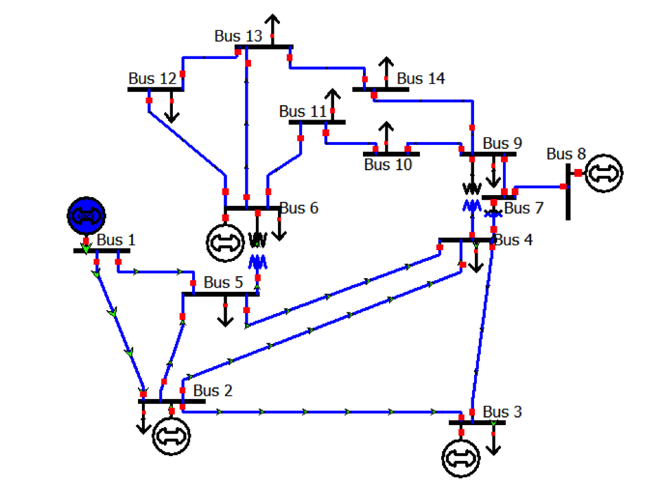
Figure 1: IEEE 14 bus test system diagram [8].

TABLE I: System Bus Information

Bus	$P_{load}$	$\sigma$	$P_{gen}^{min}$	$P_{gen}^{max}$	$C_{gen}$	$C_{reg}$
No.	(MW)	(MW)	(MW)	(MW)	($/MWh)	($/MWh)
1	34	0.68	15	332.4	21	16
2	12	0.24	15	140.0	20	11
3	9	0.18	15	100.0	35	13
4	85	1.70
5	60	1.20
6	22	0.44	15	100.0	39	12
7	103	2.06
8	30	0.60	15	100.0	40	14
9	61	1.22
10	74	1.48
11	15	0.30
12	57	1.14
13	66	1.32
14	-50	5.00

III-B Results

The results of the chance constrained DCOPF both with and without regulation reserves are compared in Table II. The economic generator dispatches and overall system costs solved for this case are given. Table III shows the calculated locational marginal prices and locational prices of variability for the cases with and without regulation reserves. The effects of the line constraint can be observed in the generator dispatches. The generators at buses 1 and 6 are dispatched at their maximum levels and the generators at buses 3 and 8 are dispatched at their minimum, accounting for the AGC reserves. These minimum dispatch generators result in lower LMPs than their offer prices. We did not consider a unit committment with this model and it may be the case that one or both of these generators may not be needed for the least-cost disptach. If they are necessary for either energy or regulation, then the difference would typically be made up via an out-of-market make whole payment to these suppliers. Note that the generator at bus 6 is more expensive than the generator at bus 3 with respect to its energy offer price. The line constraint necessitates the heavy use of this more expensive generator to supply the load in a portion of the network.

The system cost of regulation reserves for this case is small in comparison to the cost of power generation. The locational price of variability is generally smaller than the locational marginal prices for many buses where power injection variability is low. For a bus with high variability, such as the wind generator at bus 14, power injection variability costs nearly three quarters the price of electricity. The larger load at bus 7 and its higher variability contribute to its slightly higher LPV. Note that the more variable loads and generators contribute more to the combined variance in overall power fluctuations, leading to their greater impact on sensitivity studies. This expectantly leads to higher prices at those locations. The line constraint also affects the LPVs. Despite having low load variability, bus 1 also has a high LPV. At this bus regulation reserves are comparatively expensive and the generator is already operating at its generation capacity. The line constraint impedes the paths to supply balancing power for fluctuations. The prices at buses 2 and 5 are slightly elevated for similar reasons; these buses are the terminals of the congested line.

III-C Significance

We have proposed the calculation of locational prices of variability in order to allocate the costs of AGC regulation to the locations whose variabilities most impact the system. Not surprisingly, the bus locations with large variable power injections and locations which impact the constrained line have larger prices. These prices provide an incentive to reduce variations in power injections. Consider the wind generator at bus 14. As a generator it would receive revenue of 2039 ($/hr) for the supply of 50 MW, and be charged 137 ($/hr) for its variability, assuming its real-time fluctuations were similar to the expected variations. This charge amounts to almost 7 percent of its revenue. The assessment of such a charge would almost certainly warrant a cost/benefit study for the purchase of energy storage capability to reduce power fluctuations. The effect on the loads is similar but smaller because we assumed smaller fluctuations. For example, the 66 MW load at bus 13 would pay approximately 2769 ($/hr) for energy and 10 ($/hr) for variability. The added charge is less than one half of one percent of the energy charge. Nevertheless, if some load had large power fluctuations the LPV would also provide an incentive to consider energy storage or other means to smooth the power usage profile.

TABLE II: Economic Generator Dispatch

	With CC Reserves			Without CC Reserves
Generator	$P_{g}$	$A$	$\beta$	$P_{g}$
Bus No.	(MW)	(MW)	(pu)	(MW)
1	332.4	0	0	326.0
2	108.5	0.08	0.006	105.1
3	15.0	0	0	17.0
6	96.1	3.91	0.261	98.0
8	26.0	11.00	0.734	31.9
System Cost	14463	202		14641
($/hr)

TABLE III: Locational Marginal Pricing and Price of Variability

	With CC Reserves		Without CC Reserves
Bus	LMP	LPV	LMP	LPV
No.	($/MWh)	($/MWh)	($/MWh)	($/MWh)
1	25.09	28.57	25.28	1.17
2	20.00	17.13	20.00	0.99
3	29.76	4.07	30.12	0.21
4	38.20	9.99	38.87	6.59
5	44.27	10.11	45.16	10.41
6	42.29	2.75	43.11	3.06
7	39.29	11.20	40.00	9.40
8	39.29	3.26	40.00	2.95
9	39.87	6.54	40.61	6.06
10	40.30	7.96	41.05	7.81
11	41.28	1.69	42.06	1.81
12	42.10	6.97	42.91	7.63
13	41.95	7.94	42.76	8.66
14	40.78	27.35	41.55	28.15

IV Conclusion

In this paper we proposed and demonstrated a means to calculate a locational price to apply to power injection fluctuations. Our model expanded on our previous work by explicitly adding a model for AGC. This includes a market-based method for choosing generators to supply AGC in the co-optimized energy and regulation cost function. The probabilistic power flow also determined the amount of regulation reserves that are required, and the weights for the AGC controlled generators. The locational price of variability was calculated as the sensitivity of system cost to a measure of variability, in this case the standard deviation. We noted that the locations with the highest LPVs were those with either highly fluctuating power injections, or with power injections that impacted the power flow on the constrained line. We argued that the imposition of a locational charge on variability would more fairly pay for resources needed to balance load in real time. Instead of sharing the costs uniformly, the non-dispatchable resources with fluctuations that most affect system costs would be charged more for their variable power injections. These charges in turn provide an incentive to consider energy storage technologies to smooth power fluctuations.

Accepting the approach as reasonable, there are practical policy questions to consider for implementation in a market. Importantly there is a potential gap between calculating the price based on uncertainties (expectations of variability) and charging for the actual measured fluctuations. The prices presented in Table III are based on short-term expectations of nominal load, expectations of variations in load and variable renewable generation. The realizations of actual measured load, generation, and fluctuations may differ from the expectations used to calculate the prices. One could recalculate the prices ex-post, however the cost of the decision on generator dispatch was already made. There are several possible resolutions to this issue. If the history of uncertainty projections proves to match observed fluctuations well, then the method and charges can be applied as outlined in the paper. If however there are significant differences then it would make sense to dispatch generation and allocate reserves based on the best information available, and then compute prices for variability ex-post.

In either case — using prices calculated with resource allocations or prices calculated after variability is measured — the amount charged to non-dispatchable resources will likely differ from the costs of procuring regulation reserves. This is the case even with perfect projections of uncertain power injections. In our 14-bus example system, if we paid the AGC generators the highest accepted price of 14 ($/MWhr), then they would receive in total 210 ($/hr) for the allocated AGC capacity. The variable non-dispatchable loads and generation would pay in total 255 ($/hr). In this case, the sources of variable power injections would by paying 45 ($/hr) more than the AGC resources would receive and some policy would be required to handle the difference. In energy markets it is typical for loads to pay more than the the generators received due to congestion costs. In our case example using LMPS to settle payments to generators and from loads, the difference in total payments will be 8580 ($/hr). Congestion costs can be substantial and are settled using Financial Transmission Rights (FTR), for which there is a separate market. In the case of AGC, the amounts of power and the relative costs are so much smaller than the energy market that it hardly warrants a complicated structure to resolve the settlement. We recommend the price profile be used to determine the fair allocation of costs among participating entities and pro-rate the charges to cover the costs of procuring balancing power via regulation reserves. Alternatively, the small difference in payment for AGC regulation reserves could be included in the existing FTR market.

References

- [1] P. Denholm and M. Hand, “Grid flexibility and storage required to achieve very high penetration of variable renewable electricity,” Energy Policy, vol. 39, no. 3, pp. 1817–1830, 2011.
- [2] C. ISO, “What the duck curve tells us about managing a green grid,” http://www.caiso.com/Documents/FlexibleResourcesHelpRenewables_FastFacts.pdf, 2016, [Online, accessed 11-June-2017].
- [3] L. Roald, F. Oldewurtel, T. Krause, and G. Andersson, “Analytical reformulation of security constrained optimal power flow with probabilistic constraints,” in 2013 IEEE Grenoble Conference, June 2013, pp. 1–6.
- [4] T. Ding, Z. Wu, J. Lv, Z. Bie, and X. Zhang, “Corrective control to handle forecast uncertainty: A chance constrained optimal power flow,” IEEE Transactions on Sustainable Energy, vol. 7, no. 4, pp. 1547–1557, 2016.
- [5] L. Roald, S. Misra, T. Krause, and G. Andersson, “Robust co-optimization to energy and ancillary service joint dispatch considering wind power uncertainties in real-time electricity markets,” IEEE Transactions on Power Systems, vol. 32, no. 2, pp. 1626–1637, 2017.
- [6] S. Cyrus and B. C. Lesieutre, “Locational effects of variability of injected power on total cost,” in IEEE Power and Energy Conference at Illinois, 2015.
- [7] R. D. Zimmerman, C. E. Murillo-Sanchez, and R. J. Thomas, “Matpower: Steady-state operations, planning and analysis tools for power systems research and education,” IEEE Transactions on Power Systems, vol. 26, no. 1, pp. 12–19, 2011.
- [8] I. C. for a Smarter Electric Grid, “Ieee 14-bus system,” http://icseg.iti.illinois.edu/ieee-14-bus-system/, 2017, [Online, accessed 31-May-2017].