Approximation of PDE eigenvalue problems involving parameter dependent matrices

Abstract

We discuss the solution of eigenvalue problems associated with partial differential equations that can be written in the generalized form $\mathsf{A}x=\lambda\mathsf{B}x$, where the matrices $\mathsf{A}$ and/or $\mathsf{B}$ may depend on a scalar parameter. Parameter dependent matrices occur frequently when stabilized formulations are used for the numerical approximation of partial differential equations. With the help of classical numerical examples we show that the presence of one (or both) parameters can produce unexpected results.

65N30, 65N25

1 Introduction

Several schemes for the approximation of eigenvalue problems arising from partial differential equations lead to the algebraic form: find $\lambda\in\mathbb{R}$ and $x\in\mathbb{R}^{n}$ with $x\neq 0$ such that

(1) $$\mathsf{A}x=\lambda\mathsf{B}x,$$

where $\mathsf{A}$ and $\mathsf{B}$ are matrices in $\mathbb{R}^{n\times n}$.

We consider the case when the matrices $\mathsf{A}$ and $\mathsf{B}$ are symmetric and positive semidefinite and may depend on a parameter. This is a typical situation found in applications where elliptic partial differential equations are approximated by schemes that require suitable parameters to be tuned (for consistency and/or stability reasons). In this paper we discuss in particular applications arising from the use of the Virtual Element Method (VEM), see [19, 5, 15, 20, 21, 14, 22], where suitable parameters have to be chosen for the correct approximation. Similar situations are present, for instance, when a parameter-dependent stabilization is used for the approximation of discontinuous Galerkin formulations and when a penalty penalty term is added to the discretization of the eigenvalue problem associated with Maxwell’s equations [10, 12, 11, 6, 8, 26, 23, 7, 2]

In general, it may be not immediate to describe how the matrices $\mathsf{A}$ and $\mathsf{B}$ depend on the given parameters. For simplicity, we consider the case when the dependence is linear: under suitable assumptions it is easy to discuss how the computed spectrum varies with respect to the parameters.

The description of the spectrum in the linear case is not surprising and is well known to a broad scientific community [13, 25, 24, 18, 17]. Nevertheless, the main focus of perturbation theory for eigenvalues and eigenvectors is usually centered on the asymptotic behavior when the parameters tend to zero. In our case, the asymptotic parameter is usually the mesh size $h$ and we are interested in the convergence when $h$ goes to zero, that is when the size of the involved matrices tends to infinity. The presence of additional parameters makes the convergence more difficult to describe and can produce unexpected results in the pre-asymptotic regime. For this reason, we start by recalling how the spectrum of problem (1) is influhenced by the parameter, without considering $h$, and we translate those results to an example of interest in Section 3.1 where the discretization parameter $h$ is considered as well.

We assume that the matrices $\mathsf{A}$ and $\mathsf{B}$ satisfy the following condition for $\mathsf{C}=\mathsf{A},\mathsf{B}$.

Assumption 1.

The matrix $\mathsf{C}$ can be split into the sum

(2) $$\mathsf{C}=\mathsf{C}_{1}+\gamma\mathsf{C}_{2},$$

where $\gamma$ is a non negative real number and $\mathsf{C}_{1}$ and $\mathsf{C}_{2}$ are symmetric. The matrices $\mathsf{C}_{1}$ and $\mathsf{C}_{2}$ satisfy the following properties:

1. $\mathsf{C}_{1}$ is positive semidefinite with kernel $K_{\mathsf{C}_{1}}$;

2. $\mathsf{C}_{2}$ is positive semidefinite and positive definite on $K_{\mathsf{C}_{1}}$;

3. $\mathsf{C}_{2}$ vanishes on $K_{\mathsf{C}_{1}}^{\perp}$, the orthogonal complement of $K_{\mathsf{C}_{1}}$ in $\mathbb{R}^{n}$.

In Section 2 we describe the spectrum of (1) as a function of the parameters, in various situations that mimic the behavior of matrices $\mathsf{A}$ and $\mathsf{B}$ originating from several discretization schemes.

Section 3, which is the core of this paper, discusses the influence of the parameters on the VEM approximation of eigenvalue problems. Several numerical examples complete the papers, showing that the parameters have to be carefully tuned and that wrong choices can produce useless results.

2 Parametric algebraic eigenvalue problem

Given two symmetric and positive semidefinite matrices $\mathsf{A}$ and $\mathsf{B}$ that can be written as

(3) $$\mathsf{A}=\mathsf{A}_{1}+\alpha\mathsf{A}_{2}$$

and

(4) $$\mathsf{B}=\mathsf{B}_{1}+\beta\mathsf{B}_{2},$$

with nonnegative parameters $\alpha$ and $\beta$, we consider the eigensolutions to the generalized problem (1).

We assume that the splitting of the matrices $\mathsf{A}$ and $\mathsf{B}$ is obtained with symmetric matrices and satisfies 1 for $\mathsf{C}_{1}=\mathsf{A}_{1},\mathsf{B}_{1}$ and $\mathsf{C}_{2}=\mathsf{A}_{2},\mathsf{B}_{2}$. Moreover we denote by $n_{\mathsf{A}_{1}}$ and $n_{\mathsf{B}_{1}}$ the dimension of $K_{\mathsf{A}_{1}}$ and $K_{\mathsf{B}_{1}}$, respectively.

Remark 1.

Problem (1) has $n$ eigenvalues if and only if $\mathrm{rank}\mathsf{B}=n$, see [16]. If $\mathsf{B}$ is singular the spectrum can be finite, empty, or infinite (if $\mathsf{A}$ is singular too). If $\mathsf{A}$ is non singular, usually one can circumvent this difficulty by computing the eigenvalues of $\mathsf{B}x=\mu\mathsf{A}x$ and setting $\lambda=1/\mu$. The kernel of $\mathsf{B}$ is the eigenspace associated with the vanishing eigenvalue with multiplicity $m$, and the original problem has exactly $m$ eigenvalues conventionally set to $\infty$.

We want to study the behavior of the eigenvalues as the parameters $\alpha$ and $\beta$ vary. We consider three cases.

2.1 Case 1

We fix $\beta>0$ so that $\mathsf{B}$ is positive definite. This implies that the eigenvalues of (1) are all non negative. Let us consider first $\alpha=0$ so that (1) reduces to

(5) $$\mathsf{A}_{1}x=\lambda\mathsf{B}x.$$

Since $\mathsf{A}_{1}$ is positive semidefinite, $\lambda=0$ is an eigenvalue of (5) with multiplicity equal to $n_{\mathsf{A}_{1}}=\dim(K_{\mathsf{A}_{1}})$ and $K_{\mathsf{A}_{1}}$ is the associated eigenspace. In addition, we have $m_{A}=n-n_{\mathsf{A}_{1}}$ positive eigenvalues $\{\mu_{1}\leq\dots\leq\mu_{m_{A}}\}$ counted with their multiplicity (since we are dealing with a symmetric problem, we do not distinguish between geometric and algebraic multiplicity). We denote by $v_{j}\in K_{\mathsf{A}_{1}}^{\perp}$ the eigenvector associated with $\mu_{j}$, that is

$$\mathsf{A}_{1}v_{j}=\mu_{j}\mathsf{B}v_{j}.$$

Thanks to property c) of 1 when $\mathsf{C}=\mathsf{A}$, we observe that

$$\mathsf{A}v_{j}=\mathsf{A}_{1}v_{j}+\alpha\mathsf{A}_{2}v_{j}=\mathsf{A}_{1}v_{j}=\mu_{j}\mathsf{B}v_{j}.$$

Therefore $(\mu_{j},v_{j})$, for $j=1,\dots,m_{A}$, are eigensolutions of the original system (1).

On the other hand, the eigensolutions of

$$\mathsf{A}_{2}w=\nu\mathsf{B}w$$

are characterized by the fact that $n_{\mathsf{A}_{1}}$ eigenvalues $\nu_{i}$ ($i=1,\dots,n_{\mathsf{A}_{1}}$) are strictly positive with corresponding eigenvectors $w_{i}$ belonging to $K_{\mathsf{A}_{1}}$, while the remaining $m_{A}$ eigenvalues vanish and have $K_{\mathsf{A}_{1}}^{\perp}$ as eigenspace. Thus, property a) of 1, for $\mathsf{C}=\mathsf{A}$, yields

$$\mathsf{A}w_{i}=\mathsf{A}_{1}w_{i}+\alpha\mathsf{A}_{2}w_{i}=\alpha\mathsf{A}_{2}w_{i}=\alpha\nu_{i}\mathsf{B}w_{i},$$

which means that $(\alpha\nu_{i},w_{i})$, for $i=1,\dots,n_{\mathsf{A}_{1}}$, are eigensolutions of (1).

Summarizing the eigenvalues of (1) are:

(6) $$\lambda_{k}=\left\{\begin{array}[]{ll}\alpha\nu_{k}&\text{if }1\leq k\leq n_{\mathsf{A}_{1}}\\ \mu_{k-n_{\mathsf{A}_{1}}}&\text{if }n_{\mathsf{A}_{1}}+1\leq k\leq n.\end{array}\right.$$

The left panel in Fig. 1 shows the eigenvalues of a simple example where $\mathsf{A}\in\mathbb{R}^{6\times 6}$ is obtained by the combination of diagonal matrices with entries

(7) $$\operatorname{diag}(\mathsf{A}_{1})=[3,4,5,6,0,0],\quad\operatorname{diag}(\mathsf{A}_{2})=[0,0,0,0,1,2].$$

and $\mathsf{B}=\mathbb{I}_{6}$ is the identity matrix.

Along the vertical lines we see the eigenvalues corresponding to a fixed value of $\alpha$. The eigenvalues $3,4,5,6$ are associated with eigenvectors in $K_{\mathsf{A}_{1}}^{\perp}$ and do not depend on $\alpha$. The solid lines starting at the origin display the eigenvalues $1,2$ multiplied by $\alpha$.

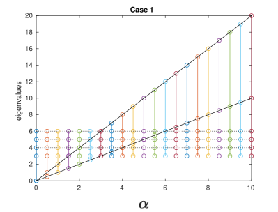
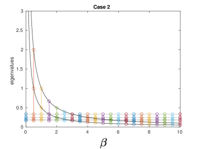
Figure 1: Dependence of the eigenvalues on the parameters $\alpha$ (Case 1) and $\beta$ (Case 2), respectively

Remark 2.

We observe that if $\mathsf{A}_{2}$ is not positive definite on $K_{\mathsf{A}_{1}}$, its kernel has a nonempty intersection with $K_{\mathsf{A}_{1}}$. Let $n_{12}$ be the dimension of this intersection, then problem (1) admits $n_{12}$ vanishing eigenvalues which appear in the first case of (6).

2.2 Case 2

Let us now fix $\alpha>0$, so that $\mathsf{A}$ is positive definite. We have that all the eigenvalues are positive. We observe that when $\beta=0$, the matrix $\mathsf{B}=\mathsf{B}_{1}$ may be singular, therefore it is convenient to consider the following problem:

(8) $$\mathsf{B}x=\chi\mathsf{A}x,$$

where $\chi=\frac{1}{\lambda}$. If $\chi=0$, we conventionally set $\lambda=\infty$. Problem (8) reproduces the same situation we had in Case 1, with the matrices $\mathsf{A}$ and $\mathsf{B}$ switched. Repeating the same arguments as before, we obtain that problem (8) has two families of eigenvalues

$$\chi_{k}=\left\{\begin{array}[]{ll}\beta\xi_{k}&\text{if }1\leq k\leq n_{\mathsf{B}_{1}}\\ \zeta_{k-n_{\mathsf{B}_{1}}}&\text{if }n_{\mathsf{B}_{1}}+1\leq k\leq n,\end{array}\right.$$

where

$$\mathsf{B}_{1}r_{j}=\zeta_{j}\mathsf{A}r_{j},\ j=1,\dots,n-n_{\mathsf{B}_{1}} \text{ with }r_{j}\in K_{\mathsf{B}_{1}}^{\perp}$$

$$\mathsf{B}_{2}s_{i}=\xi_{i}\mathsf{A}s_{i},\ i=1,\dots,n_{\mathsf{B}_{1}} \text{ with }s_{i}\in K_{\mathsf{B}_{1}}.$$

Going back to the original problem (1), we can conclude that the eigensolutions of (1) are the following ones:

(9) $$\left(\frac{1}{\beta\xi_{k}},s_{k}\right) \text{ for }k=1,\dots,n_{\mathsf{B}_{1}}$$

$$\left(\frac{1}{\zeta_{k-n_{\mathsf{B}_{1}}}},r_{k-n_{\mathsf{B}_{1}}}\right) \text{ for }k=n_{\mathsf{B}_{1}}+1,\dots,n.$$

In the right panel of Fig. 1, we report the eigenvalues of a simple example where $\mathsf{A}=\mathbb{I}_{6}$ and $\mathsf{B}$ is obtained by combining $\mathsf{B}_{1}=\mathsf{A}_{1}$ and $\mathsf{B}_{2}=\mathsf{A}_{2}$ defined in (7). We see that the eigenvalues $\frac{1}{3},\frac{1}{4},\frac{1}{5},\frac{1}{6}$ are independent of $\beta$ and that the remaining two eigenvalues lie along the hyperbolas $\frac{1}{\beta}$ and $\frac{1}{2\beta}$, plotted with solid line.

2.3 Case 3

We consider now the case when $\alpha$ and $\beta$ can vary independently from each other. We have different situations corresponding to the relation between $K_{\mathsf{A}_{1}}$ and $K_{\mathsf{B}_{1}}$. To ease the reading, let us introduce the following notation:

(10a) $$\mathsf{A}_{1}v=\mu\mathsf{B}_{1}v$$

(10b) $$\mathsf{A}_{1}w=\nu\mathsf{B}_{2}w$$

(10c) $$\mathsf{A}_{2}y=\chi\mathsf{B}_{1}y$$

(10d) $$\mathsf{A}_{2}z=\eta\mathsf{B}_{2}z.$$

In this case the space $\mathbb{R}^{n}$ can be decomposed into four mutually orthogonal subspaces

$$\mathbb{R}^{n}=(K_{\mathsf{A}_{1}}\cap K_{\mathsf{B}_{1}})\oplus(K_{\mathsf{A}_{1}}\cap K_{\mathsf{B}_{1}}^{\perp})\oplus(K_{\mathsf{A}_{1}}^{\perp}\cap K_{\mathsf{B}_{1}})\oplus(K_{\mathsf{A}_{1}}^{\perp}\cap K_{\mathsf{B}_{1}}^{\perp}).$$

Let us denote by $n_{\mathsf{A}_{1}\cap\mathsf{B}_{1}}$ the dimension of $K_{\mathsf{A}_{1}}\cap K_{\mathsf{B}_{1}}$. If $K_{\mathsf{A}_{1}}\cap K_{\mathsf{B}_{1}}\neq\emptyset$, for $x\in K_{\mathsf{A}_{1}}\cap K_{\mathsf{B}_{1}}$ the eigenproblem to be solved is $\alpha\mathsf{A}_{2}x=\lambda\beta\mathsf{B}_{2}x$, hence the eigenvalues are given by $\frac{\alpha}{\beta}\eta_{i}$ $i=1,\dots,n_{\mathsf{A}_{1}\cap\mathsf{B}_{1}}$, see (10d). Next, if $x\in K_{\mathsf{A}_{1}}\cap K_{\mathsf{B}_{1}}^{\perp}$ we have to solve $\alpha\mathsf{A}_{2}x=\lambda\mathsf{B}_{1}x$, which admits $(\alpha\chi_{i},y_{i})$ $i=1,\dots,n_{\mathsf{A}_{1}}-n_{\mathsf{A}_{1}\cap\mathsf{B}_{1}}$ as eigensolutions where $(\chi_{i},y_{i})$ are defined in (10c). Similarly, if $x\in K_{\mathsf{A}_{1}}^{\perp}\cap K_{\mathsf{B}_{1}}$, we find that the eigensolutions are $\left(\frac{1}{\beta}\nu_{i},w,_{i}\right)$ $i=1,\dots,n_{\mathsf{B}_{1}}-n_{\mathsf{A}_{1}\cap\mathsf{B}_{1}}$ with $(\nu_{i},w_{i})$ given by (10b). In the last case, $x\in K_{\mathsf{A}_{1}}^{\perp}\cap K_{\mathsf{B}_{1}}^{\perp}$, the matrices $\mathsf{A}$ and $\mathsf{B}$ are non singular and thanks to property c) in  1, for $\mathsf{C}=\mathsf{A}$ and $\mathsf{C}=\mathsf{B}$, we obtain that the eigenvalues are positive and independent of $\alpha$ and $\beta$ and correspond to those of (10a). In conclusion, we have

$$\lambda_{k}=\left\{\begin{array}[]{ll}\displaystyle\frac{\alpha}{\beta}\eta_{k}&\quad\text{ if }1\leq k\leq n_{\mathsf{A}_{1}\cap\mathsf{B}_{1}}\\ \alpha\chi_{k-n_{\mathsf{A}_{1}\cap\mathsf{B}_{1}}}&\quad\text{ if }n_{\mathsf{A}_{1}\cap\mathsf{B}_{1}}+1\leq k\leq n_{\mathsf{A}_{1}}\\ \displaystyle\frac{1}{\beta}\nu_{k-n_{\mathsf{A}_{1}}}&\quad\text{ if }n_{\mathsf{A}_{1}}+1\leq k\leq n_{\mathsf{A}_{1}}+n_{\mathsf{B}_{1}}-n_{\mathsf{A}_{1}\cap\mathsf{B}_{1}}\\ \mu_{k-n_{\mathsf{A}_{1}}+n_{\mathsf{B}_{1}}-n_{\mathsf{A}_{1}\cap\mathsf{B}_{1}}}&\quad\text{ if }n_{\mathsf{A}_{1}}+n_{\mathsf{B}_{1}}-n_{\mathsf{A}_{1}\cap\mathsf{B}_{1}}+1\leq k\leq n.\end{array}\right.$$

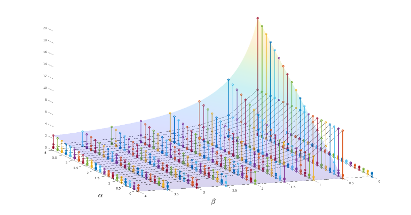
Figure 2: Eigenvalues when $K_{\mathsf{A}_{1}}\cap K_{\mathsf{B}_{1}}\neq\emptyset$ as a function of $\alpha$ and $\beta$

We report in Fig. 2 the eigenvalues illustrating this last case when we have diagonal matrices given by

$$\operatorname{diag}(\mathsf{A}_{1})=[3,0,0,4,5,6] \quad\operatorname{diag}(\mathsf{A}_{2})=[0,1,2,0,0,0]$$

$$\operatorname{diag}(\mathsf{B}_{1})=[7,8,0,0,9,10] \quad\operatorname{diag}(\mathsf{B}_{2})=[0,0,0.8,1,0,0].$$

The surface contains the eigenvalues depending on both $\alpha$ and $\beta$, the hyperbolas those depending only on $\beta$ and the straight lines those depending only on $\alpha$. If we cut the three dimensional picture with a plane at $\beta>0$ fixed we recognize the behavior analyzed in Section 2.1 and shown in Fig. 1 left. Analogously, taking a plane with $\alpha>0$ fixed, we recover Case 2 (see Section 2.2).

If $K_{\mathsf{A}_{1}}\cap K_{\mathsf{B}_{1}}=\emptyset$, we set $n_{\mathsf{A}_{1}\cap\mathsf{B}_{1}}=0$, hence the eigenvalues are

$$\lambda_{k}=\left\{\begin{array}[]{ll}\alpha\chi_{k}&\text{ if }1\leq k\leq n_{\mathsf{A}_{1}}\\ \displaystyle\frac{1}{\beta}{\nu_{k-n_{\mathsf{A}_{1}}}}&\text{ if }n_{\mathsf{A}_{1}}+1\leq k\leq n_{\mathsf{A}_{1}}+n_{\mathsf{B}_{1}}\\ \mu_{k-n_{\mathsf{A}_{1}}-n_{\mathsf{B}_{1}}}&\text{ if }n_{\mathsf{A}_{1}}+n_{\mathsf{B}_{1}}+1\leq k\leq n\end{array}.\right.$$

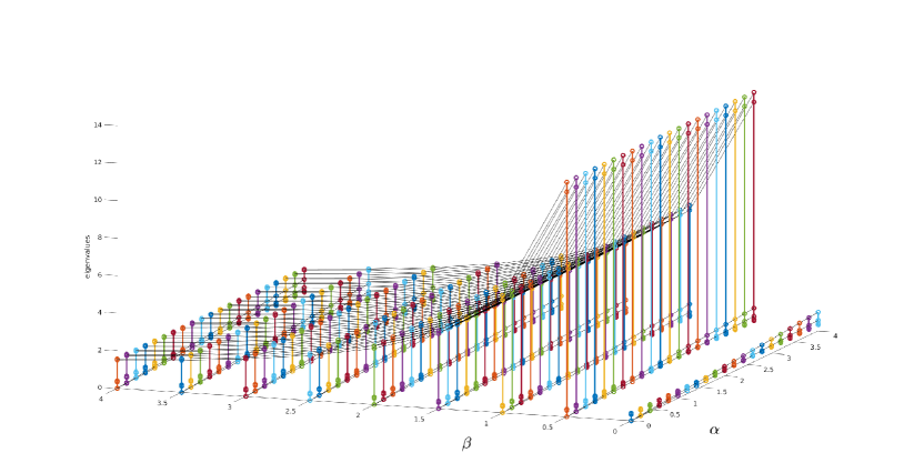
Figure 3: Eigenvalues when $K_{\mathsf{A}_{1}}\cap K_{\mathsf{B}_{1}}=\emptyset$ as a function of $\alpha$ and $\beta$

In order to illustrate the case $K_{\mathsf{A}_{1}}\cap K_{\mathsf{B}_{1}}=\emptyset$, we report in Fig. 3 the eigenvalues computed using the following diagonal matrices with entries

$$\operatorname{diag}(\mathsf{A}_{1})=[0,0,3,4,5,6], \quad\operatorname{diag}(\mathsf{A}_{2})=[1,2,0,0,0,0],$$

$$\operatorname{diag}(\mathsf{B}_{1})=[7,8,9,10,0,0], \quad\operatorname{diag}(\mathsf{B}_{2})=[0,0,0,0,0.8,1].$$

For a fixed $\alpha$, we can see in solid line the hyperbolas $\frac{\nu_{j}}{\beta}$, $j=1,2$ while when $\beta$ is fixed we can see the straight lines $\alpha\chi_{j}$, $j=1,2$. The remaining two eigenvalues are independent of $\alpha$ and $\beta$.

3 Virtual element method for eigenvalue problems

In this section we recall how algebraic eigenvalue problems similar to the ones discussed in the previous section can be obtained withing the framework of the Virtual Element Method (VEM) for the discretization of elliptic eigenvalue problems, see [15, 14].

We consider the model problem of the Laplacian operator. Given a connected open domain with Lipschitz continuous boundary $\Omega\subseteq\mathbb{R}^{d}$, with $d=2,3$, we look for eigenvalues $\lambda\in\mathbb{R}$ and eigenfunctions $u\neq 0$ such that

$$\left\{\begin{array}[]{ll}-\Delta u=\lambda u&\quad\text{ in }\Omega\\ u=0&\quad\text{ on }\partial\Omega.\end{array}\right.$$

In view of the application of VEM, we consider the weak form: find $\lambda\in\mathbb{R}$ and $u\in H^{1}_{0}(\Omega)$ with $u\neq 0$ such that

(11) $$a(u,v)=\lambda b(u,v)\quad\forall v\in H^{1}_{0}(\Omega),$$

where

$$a(u,v)=(\nabla u,\nabla v),\quad b(u,v)=(u,v),$$

and $(\cdot,\cdot)$ is the scalar product in $L^{2}(\Omega)$.

It is well-known that problem (11) admits an infinite sequence of positive eigenvalues

$$0<\lambda_{1}\leq\dots\leq\lambda_{i}\leq\cdots$$

repeated according to their multiplicity, each one associated with an eiegenfunction $u_{i}$ with the following properties

(12) $$a(u_{i},u_{j})=b(u_{i},u_{j})=0\quad\text{if }i\neq j$$

$$b(u_{i},u_{i})=1,\quad a(u_{i},u_{i})=\lambda_{i}.$$

Let us briefly recall the definition of the virtual element spaces and of the discrete bilinear forms which we are going to use in this section, see [3, 1]. We present only the two dimensional spaces, the three dimensional ones are obtained using the 2D virtual elements on the faces.

We decompose $\Omega$ into polygons $P$, with diameter $h_{P}$ and area $|P|$. Similarly, if $e$ is an edge of an element $P$, we denote by $h_{e}=|e|$ its length. Depending on the context $\partial P$ refers to either the boundary of $P$ or the set of the edges of $P$. The notation $\mathcal{T}_{h}$ and $\mathcal{E}_{h}$ stands for the set of the elements and the edges, respectively. As usual, $h=\max_{P\in\mathcal{T}_{h}}h_{P}$. We assume the following mesh regularity condition (see [3]): there exists a positive constant $\gamma$, independent of $h$, such that each element $P\in\mathcal{T}_{h}$ is star-shaped with respect to a ball of radius greater than $\gamma h_{P}$; moreover, for every element $P$ and for every edge $e\subset\partial P$, it holds $h_{e}\geq\gamma h_{P}$.

For $k\geq 1$ and $P\in\mathcal{T}_{h}$ we define

$$\tilde{V}_{h}^{k}(P)=\{v\in H^{1}(P):v|_{\partial P}\in C^{0}(\partial P),v|_{e}\in\mathbb{P}_{k}(e)\ \forall e\subset\partial P,\Delta v\in\mathbb{P}_{k}(P)\}.$$

We consider the following linear forms on the space $\tilde{V}_{h}^{k}(P)$

1. : the values $v(V_{i})$ at the vertices $V_{i}$ of $P$,

2. : the scaled edge moments up to order $k-2$

   $$\dfrac{1}{|e|}\int_{e}vm\,\text{d}s\quad\forall m\in\mathcal{M}_{k-2}(e),\ \forall e\subset\partial P,$$

3. : the scaled element moments up to order $k-2$

   $$\dfrac{1}{|P|}\int_{P}vm\,\text{d}x\quad\forall m\in\mathcal{M}_{k-2}(P),\$$

where $\mathcal{M}_{k-2}(\omega)$ is the set of scaled monomials on $\omega$, namely

$$\mathcal{M}_{k-2}(\omega)=\Big{\{}\Big{(}\dfrac{\mathbf{x}-\mathbf{x}_{\omega}}{h_{\omega}}\Big{)}^{s},|s|\leq k-2\Big{\}},$$

with $\mathbf{x}_{\omega}$ the barycenter of $\omega$, and with the convention that $\mathcal{M}_{-1}(\omega)=\emptyset$.

From the values of the linear operators D1–D3, on each element $P$ we can compute a projection operator $\Pi_{k}^{\nabla}:\tilde{V}_{h}^{k}(P)\rightarrow\mathbb{P}_{k}(P)$ defined as the unique solution of the following problem:

(13) $$a^{P}(\Pi_{k}^{\nabla}v-v,p)=0\quad\forall p\in\mathbb{P}_{k}(P)$$

$$\int_{\partial P}(\Pi_{k}^{\nabla}v-v)\text{d}s=0,$$

where $a^{P}(u,v)=(\nabla u,\nabla v)_{P}$ and $(\cdot,\cdot)_{P}$ denotes the $L^{2}(P)$-scalar product.

The local virtual space is defined as

(14) $$V_{h}^{k}(P)=\left\{v\in\tilde{V}_{h}^{k}(P):\int_{P}(v-\Pi_{k}^{\nabla}v)p\text{d}x=0\ \forall p\in(\mathbb{P}_{k}\setminus\mathbb{P}_{k-2})(P)\right\},$$

where $(\mathbb{P}_{k}\setminus\mathbb{P}_{k-2})(P)$ contains the polynomials in $\mathbb{P}_{k}(P)$ $L^{2}$-orthogonal to $\mathbb{P}_{k-2}(P)$.

We recall that by construction $\mathbb{P}_{k}(P)\subset V_{h}^{k}(P)$, so that the optimal rate of convergence is ensured. Moreover, the linear operators D1–D3 provide a unisolvent set of degrees of freedom (DoFs) for $V_{h}^{k}(P)$, which allows us to define and compute $\Pi_{k}^{\nabla}$ on $V_{h}^{k}(P)$. In addition, the $L^{2}$-projection operator $\Pi^{0}_{k}:V_{h}^{k}(P)\to\mathbb{P}_{k}(P)$ is also computable using the DoFs.

The global virtual space is

(15) $$V_{h}^{k}=\{v\in H^{1}_{0}(\Omega):v|_{P}\in V_{h}^{k}(P)\ \forall P\in\mathcal{T}_{h}\}.$$

In order to discretize problem (11), we introduce the discrete counterparts $a_{h}$ and $b_{h}$ of the bilinear forms $a$ and $b$, respectively. Both discrete forms are obtained as sum of the following local contributions: for all $u_{h},v_{h}\in V_{h}^{k}$

(16) $$a_{h}^{P}(u_{h},v_{h})=a^{P}(\Pi_{k}^{\nabla}u_{h},\Pi_{k}^{\nabla}v_{h})+S_{a}^{P}((I-\Pi_{k}^{\nabla})u_{h},(I-\Pi_{k}^{\nabla})v_{h})$$

$$b_{h}^{P}(u_{h},v_{h})=b^{P}(\Pi^{0}_{k}u_{h},\Pi^{0}_{k}v_{h})+S_{b}^{P}((I-\Pi^{0}_{k})u_{h},(I-\Pi^{0}_{k})v_{h}),$$

where $b^{P}(u,v)=(u,v)_{P}$, and $S_{a}^{P}$ and $S_{b}^{P}$ are symmetric positive definite bilinear forms on $V_{h}^{k}(P)\times V_{h}^{k}(P)$ such that

(17) $$c_{0}a^{P}(v,v)\leq S_{a}^{P}(v,v)\leq c_{1}a^{P}(v,v) \quad\forall v\in V_{h}^{k}(P)\text{ with }\Pi_{k}^{\nabla}v=0$$

$$c_{2}b^{P}(v,v)\leq S_{b}^{P}(v,v)\leq c_{3}b^{P}(v,v) \quad\forall v\in V_{h}^{k}(P)\text{ with }\Pi^{0}_{k}v=0,$$

for some positive constants $c_{i}$ ($i=0,\dots,3$) independent of $h$. We define $a_{h}(u_{h},v_{h})=\sum_{P\in\mathcal{T}_{h}}a_{h}^{P}(u_{h},v_{h})$ and $b_{h}(u_{h},v_{h})=\sum_{P\in\mathcal{T}_{h}}b_{h}^{P}(u_{h},v_{h})$.

The virtual element counterpart of (11) reads: find $\lambda_{h}$ and $u_{h}\in V_{h}^{k}$ with $u_{h}\neq 0$ such that

(18) $$a_{h}(u_{h},v_{h})=\lambda_{h}b_{h}(u_{h},v_{h})\quad\forall v_{h}\in V_{h}^{k}.$$

Thanks to (17), the discrete problem (18) admits $N_{h}=\dim{V_{h}^{k}}$ positive eigenvalues

$$0<\lambda_{1h}\leq\dots\lambda_{N_{h}h}$$

and the corresponding eigenfunctions $u_{ih}$, for $i=1,\dots,N_{h}$, enjoy the discrete counterpart of properties in (12).

The following convergence result has been proved in [15].

Theorem 1.

Let $\lambda$ be an eigenvalue of (11) of multiplicity $m$ and $\mathcal{E}_{\lambda}$ the corresponding eigenspace. Then there are exactly $m$ discrete eigenvalues of (18) $\lambda_{j(i)h}$ ($i=1,\dots,m$) tending to $\lambda$. Moreover, assuming that $u\in H^{1+r}(\Omega)$, for all $u\in\mathcal{E}_{\lambda}$, the following inequalities hold true:

$$|\lambda-\lambda_{j(i)h}|\leq Ch^{2t}$$

$$\hat{\delta}(\mathcal{E}_{\lambda},\oplus_{i}\mathcal{E}_{j(i)h})\leq Ch^{t},$$

where $t=\min(k,r)$, $\hat{\delta}(\mathcal{E},\mathcal{F})$ represents the gap between the spaces $\mathcal{E}$ and $\mathcal{F}$, and $\mathcal{E}_{\ell h}$ is the eigenspace spanned by $u_{\ell h}$.

Remark 3.

It is also possible to consider on the right hand side of (18) the bilinear form for $\tilde{b}_{h}(u_{h},v_{h})=\sum_{P\in\mathcal{T}_{h}}b^{P}(\Pi^{0}_{k}u_{h},\Pi^{0}_{k}v_{h})$. This leads to the following discrete eigenvalue problem: find $(\tilde{\lambda}_{h},\tilde{u}_{h})\in\mathbb{R}\times V_{h}^{k}$ with $\tilde{u}_{h}\neq 0$ such that

(19) $$a_{h}(\tilde{u}_{h},v_{h})=\tilde{\lambda}_{h}\tilde{b}_{h}(\tilde{u}_{h},v_{h})\quad\forall v_{h}\in V_{h}^{k}.$$

The analogue of 1 holds true for this partially non stabilized discretization as well.

3.1 Computational aspects and numerical results

In order to compute the solution of problems (18) and (19), we need to describe how to obtain the matrices associated to our bilinear forms. By construction the matrix $\mathsf{A}_{1}$ (respectively, $\mathsf{B}_{1}$) associated with $\sum_{P}a^{P}(\Pi_{k}^{\nabla}\cdot,\Pi_{k}^{\nabla}\cdot)$ (respectively, $\sum_{P}b^{P}(\Pi^{0}_{k}\cdot,\Pi^{0}_{k}\cdot)$) has kernel corresponding to the elements $v_{h}\in V_{h}^{k}$ such that $\Pi_{k}^{\nabla}v_{h}$ is constant (respectively, $\Pi^{0}_{k}v_{h}=0$) for all $P\in\mathcal{T}_{h}$.

We observe that the local contributions of the bilinear forms displayed in (16) mimic the following exact relations

(20) $$a^{P}(u_{h},v_{h})=a^{P}(\Pi_{k}^{\nabla}u_{h},\Pi_{k}^{\nabla}v_{h})+a^{P}((I-\Pi_{k}^{\nabla})u_{h},(I-\Pi_{k}^{\nabla})v_{h})$$

$$b^{P}(u_{h},v_{h})=b^{P}(\Pi^{0}_{k}u_{h},\Pi^{0}_{k}v_{h})+b^{P}((I-\Pi^{0}_{k})u_{h},(I-\Pi^{0}_{k})v_{h}).$$

Let us denote by $\mathsf{A}^{\ell}_{1}$, $\mathsf{A}^{\ell}_{2}$, $\mathsf{B}^{\ell}_{1}$ and $\mathsf{B}^{\ell}_{2}$ the matrices whose entries are given by

(21) $$(\mathsf{A}^{\ell}_{1})_{ij}=a^{P}(\Pi_{k}^{\nabla}\phi_{i},\Pi_{k}^{\nabla}\phi_{j}), (\mathsf{A}^{\ell}_{2})_{ij}=a^{P}((I-\Pi_{k}^{\nabla})\phi_{i},(I-\Pi_{k}^{\nabla})\phi_{j})$$

$$(\mathsf{B}^{\ell}_{1})_{ij}=b^{P}(\Pi^{0}_{k}\phi_{i},\Pi^{0}_{k}\phi_{j}), (\mathsf{B}^{\ell}_{2})_{ij}=b^{P}((I-\Pi^{0}_{k})\phi_{i},(I-\Pi^{0}_{k})\phi_{j})$$

with $\phi_{i}$ basis functions for $V_{h}^{k}(P)$.

Even if the global matrices $\mathsf{A}$ and $\mathsf{B}$ do not satisfy the properties stated in 1, it turns out that 1 is fulfilled by $\mathsf{C}=\mathsf{B}^{\ell}_{1}+\beta\mathsf{B}^{\ell}_{2}$; moreover, $\mathsf{C}=\mathsf{A}^{\ell}_{1}+\alpha\mathsf{A}^{\ell}_{2}$ is characterized by the situation described in Remark 2.

We start with the pair $\mathsf{A}^{\ell}_{1}$ and $\mathsf{A}^{\ell}_{2}$. The kernel $K_{\mathsf{A}^{\ell}_{1}}$, with abuse of notation, is characterized by

$$K_{\mathsf{A}^{\ell}_{1}}=\{v\in V_{h}^{k}(P):a^{P}(\Pi_{k}^{\nabla}v,\Pi_{k}^{\nabla}w)=0\ \forall w\in V_{h}^{k}(P)\},$$

that is, $K_{\mathsf{A}^{\ell}_{1}}$ is made of $v$ with constant $\Pi_{k}^{\nabla}v$ on $P$. Moreover, the orthogonal complement of $K_{\mathsf{A}^{\ell}_{1}}$, denoted by $K_{\mathsf{A}^{\ell}_{1}}^{\perp}$ contains the elements $v\in V_{h}^{k}(P)$ such that $a^{P}(v,w)=0$ for all $w\in K_{\mathsf{A}^{\ell}_{1}}$.

We now show that $\mathsf{A}^{\ell}_{2}(K_{\mathsf{A}^{\ell}_{1}}^{\perp})=0$, that is, for all $v\in K_{\mathsf{A}^{\ell}_{1}}^{\perp}$, $a^{P}((I-\Pi_{k}^{\nabla})v,(I-\Pi_{k}^{\nabla})w)=0$ for all $w\in V_{h}^{k}(P)$. We recall that, if $v\in K_{\mathsf{A}^{\ell}_{1}}^{\perp}$, then $a^{P}(v,w)=0$ for all $w\in K_{\mathsf{A}^{\ell}_{1}}$. This implies that for $v\in K_{\mathsf{A}^{\ell}_{1}}^{\perp}$ and $w\in K_{\mathsf{A}^{\ell}_{1}}$, it holds true that $a^{P}(v,w)=a^{P}((I-\Pi_{k}^{\nabla})v,(I-\Pi_{k}^{\nabla})w)=0$. Now we can write for all $w\in V_{h}^{k}(P)$

$$a^{P}((I-\Pi_{k}^{\nabla})v,(I-\Pi_{k}^{\nabla})w)$$

$$\quad=a^{P}((I-\Pi_{k}^{\nabla})v,(I-\Pi_{k}^{\nabla})(I-\Pi_{k}^{\nabla})w)+a^{P}((I-\Pi_{k}^{\nabla})v,(I-\Pi_{k}^{\nabla})\Pi_{k}^{\nabla}w)=0.$$

Indeed, $\Pi_{k}^{\nabla}(I-\Pi_{k}^{\nabla})w=0$ implies that $(I-\Pi_{k}^{\nabla})w\in K_{\mathsf{A}^{\ell}_{1}}$, and thus the first term vanishes, while for the second term it is enough to observe that $\Pi_{k}^{\nabla}(\Pi_{k}^{\nabla}w)=\Pi_{k}^{\nabla}w$. Thus property c) of 1 is verified for $\mathsf{C}=\mathsf{A}$.

Concerning property b) of 1, we have by construction, that $a^{P}((I-\Pi_{k}^{\nabla})v,(I-\Pi_{k}^{\nabla})v)\geq 0$ for all $v\in V_{h}^{k}(P)$, see (20). On the other hand, if $v$ is constant on $P$, then $\Pi_{k}^{\nabla}v=v$ is constant, therefore $v\in K_{\mathsf{A}^{\ell}_{1}}$ and $(I-\Pi_{k}^{\nabla})v=0$ so that $v$ belongs also to the kernel of $\mathsf{A}^{\ell}_{2}$. Hence the pair $\mathsf{A}^{\ell}_{1}$ and $\mathsf{A}^{\ell}_{2}$ does not satisfy property b), but it is in the situation described in Remark 2.

Let us now consider the pair $\mathsf{B}^{\ell}_{1}$ and $\mathsf{B}^{\ell}_{2}$. We observe that the kernel of $\mathsf{B}^{\ell}_{1}$ is characterized by $\Pi^{0}_{k}v=0$. The analysis performed for the pair $\mathsf{A}^{\ell}_{1}$ and $\mathsf{A}^{\ell}_{2}$ can be repeated and gives that in this case 1 is verified for $\mathsf{C}=\mathsf{B}$.

As a consequence of the assembling of the local matrices, the global matrices $\mathsf{A}_{1}$ and $\mathsf{A}_{2}$ ($\mathsf{B}_{1}$ and $\mathsf{B}_{2}$, respectively) do not satisfy anymore the properties listed in 1. In particular, for $k=1$ we shall see that the matrices $\mathsf{A}_{1}$ and $\mathsf{B}_{1}$ are not singular. Nevertheless, we are going to show that the numerical results look pretty much similar to the ones reported in Section 2.

Moreover, in practice the matrices $\mathsf{A}^{\ell}_{2}$ and $\mathsf{B}^{\ell}_{2}$ are not available and they are replaced by using the local bilinear forms $S_{a}^{P}$ and $S_{b}^{P}$ given in (16) as follows.

Let us denote by $\mathbf{u}_{h},\mathbf{v}_{h}\in\mathbb{R}^{N_{P}}$ the vectors containing the values of the $N_{P}$ local DoFs associated to $u_{h},v_{h}\in V_{h}^{k}(P)$. Then, we define the local stabilized forms as

$$S_{a}^{P}(u_{h},v_{h})=\sigma_{P}\mathbf{u}_{h}^{\top}\mathbf{v}_{h},\quad S_{b}^{P}(u_{h},v_{h})=\tau_{P}h_{P}^{2}\mathbf{u}_{h}^{\top}\mathbf{v}_{h}$$

where the stability parameters $\sigma_{P}$ and $\tau_{P}$ are positive constants which might depend on $P$ but are independent of $h$. We point out that this choice implies the stability requirements in (17). In the applications, the parameter $\sigma_{P}$ is usually chosen depending on the mean value of the eigenvalues of the matrix stemming from the term $a_{P}(\Pi_{k}^{\nabla}\cdot,\Pi_{k}^{\nabla}\cdot)$, and $\tau_{P}$ as the mean value of the eigenvalues of the matrix resulting from $\frac{1}{h^{2}_{P}}(\Pi^{0}_{k}\cdot,\Pi^{0}_{k}\cdot)_{P}$. The choice of the stabilized form $S_{a}^{P}$ is discussed in some papers concerning the source problem, see, e.g., [4] and the references therein. One can find an analysis of the stabilization parameters $\sigma_{P}$ in [9].

If $\sigma_{P}$ and $\tau_{P}$ vary in a small range, it is reasonable to take $\sigma_{P}=\alpha$ and $\tau_{P}=\beta$ for all $P$ and this is the situation which we discuss further. Therefore, the structure of the matrices is $\mathsf{A}=\mathsf{A}_{1}+\alpha\mathsf{A}_{2}$ and $\mathsf{B}=\mathsf{B}_{1}+\beta\mathsf{B}_{2}$ where $\mathsf{A}_{2}$ and $\mathsf{B}_{2}$ are the matrices with local contribution given by $\mathbf{u}_{h}^{\top}\mathbf{v}_{h}$ and $h_{P}^{2}\mathbf{u}_{h}^{\top}\mathbf{v}_{h}$, respectively. We study the behavior of the eigenvalues as $\alpha$ and $\beta$ vary in given ranges.

In the following tests $\Omega$ is the unit square partitioned using a sequence of Voronoi meshes with a given number of elements. In Fig. 4 we report the coarsest mesh with 50 elements ($h=0.2350$, 151 edges, 102 vertices). We recall that the exact eigenvalues are given by $(i^{2}+j^{2})\pi^{2}$ for $i,j\in\mathbb{N}\setminus\{0\}$ with eigenfunctions $\sin(i\pi x)\sin(j\pi y)$. The following numerical results have been obtained using Matlab and, in particular, the routine eig for the computation of the eigenvalues. In the following figures, we shall always report the computed eigenvalues divided by $\pi^{2}$.

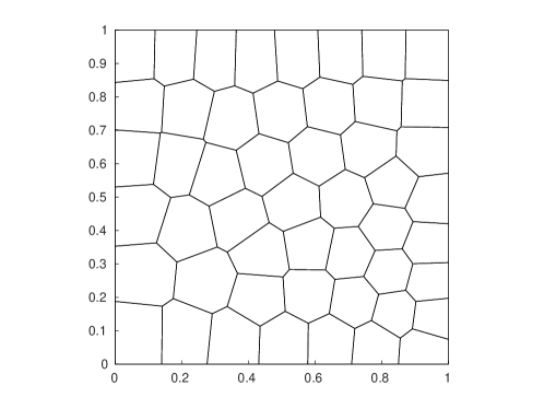
Figure 4: Voronoi mesh with 50 polygons.

Table 1 and Table 2 display the dimension of the kernel of the matrices $\mathsf{A}_{1}$ and $\mathsf{B}_{1}$ for $k=1,2,3$, and for different numbers $N$ of the elements in the mesh.

Table 1: Dimension of $K_{\mathsf{A}_{1}}$ with respect to $k$ and the number of elements

$k$		$N=50$		$N=100$		$N=200$		$N=400$		$N=800$
1		0		0		0		0		0
2		3		30		99		258		565
3		27		94		246		588		1312

Table 2: Dimension of $K_{\mathsf{B}_{1}}$ with respect to $k$ and the number of elements

$k$		$N=50$		$N=100$		$N=200$		$N=400$		$N=800$
1		0		0		0		0		0
2		0		0		0		0		0
3		0		1		43		182		504

In particular we see that for $k=1$ the matrix $\mathsf{A}_{1}$ is nonsingular.

We have computed the lowest eigenvalue of $\mathsf{A}_{1}x=\lambda\mathsf{B}_{1}x$, which gives an estimate of the inf-sup constant of the discrete problem (18). The results, presented in Table 3, show that the first eigenvalue is decreasing, and this behavior corresponds to the fact that the bilinear form $\sum_{P}a^{P}(\Pi_{k}^{\nabla}\cdot,\Pi_{k}^{\nabla}\cdot)$ is not stable.

Table 3: First eigenvalues of $\mathsf{A}_{1}x=\lambda\mathsf{B}_{1}x$ for different meshes

$N=50$	$N=100$	$N=200$	$N=400$	$N=800$
1.92654e+00	1.74193e+00	1.06691e+00	6.81927e-01	5.54346e-01

We now discuss some tests, where we present the behavior of the eigenvalues as the parameters $\alpha$ and $\beta$ vary, for the mesh with $N=200$ and different degree $k$ of the polynomials in the space $V_{h}^{k}$.

The rows of Fig. 5 contain the results for fixed $k$ and the values $\beta=0,1,5$, while, in the columns, $\beta$ is fixed and $k$ varies. In each picture, we plot in red the exact eigenvalues and with different colors those corresponding to $\alpha=10^{r}$ with $r=-3,\dots,1$.

These plots clearly confirm that the choice of the parameters for optimal performance is not so immediate. Consider, in particular, that we are solving the Laplace eigenvalue problem (isotropic diffusion) on a domain as simple as a square. For an arbitrary elliptic problem and more general domains the situation could be much more complicated. For $\beta=0$, the first 30 eigenvalues are well approximated with higher degree of polynomials whenever $\alpha\geq 0.1$. The value $\alpha=0.1$ seems to be the best choice in the case $k=1$. Increasing $\beta$ does not produce much improvement. All the pictures seem to indicate that higher values of $\alpha$ might give better results. In particular, for $k=2,3$ the first 30 eigenvalues are approximated with a reasonable accuracy for $\alpha=10$ and $\beta=1$. Increasing $\beta$ and keeping $\alpha=10$, we see that a smaller number of eigenvalues are captured.

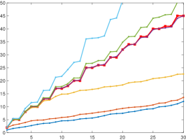
(a) $k=1$, $\beta=0$

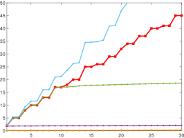
(b) $k=1$, $\beta=1$

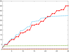
(c) $k=1$, $\beta=5$

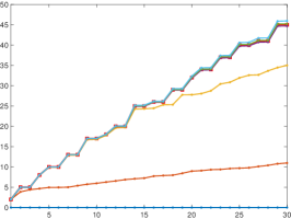
(d) $k=2$, $\beta=0$

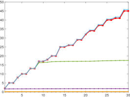
(e) $k=2$, $\beta=1$

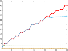
(f) $k=2$, $\beta=5$

(g) $k=3$, $\beta=0$

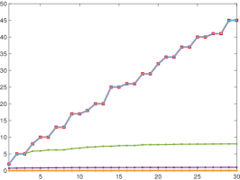
(h) $k=3$, $\beta=1$

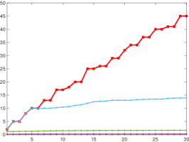
(i) $k=3$, $\beta=5$

Figure 5: First 30 eigenvalues for different values of $k$, $\alpha$ and $\beta$

Figure 6 shows the behavior of the eigenvalues as $\alpha$ varies from $0$ to $10$. At a first glance the pictures remind of Fig. 1 (left) even if, as it has been explained before, the situation is not exactly matching what we discussed in Section 2.

Each subplot reports all computed eigenvalues between $0$ and $40$; the dotted horizontal lines represent the exact solutions. The first $30$ computed eigenvalues are connected together with lines of different colors in an automated way. An “ideal” good approximation would correspond to a series of colored lines matching the dotted lines of the exact eigenvalues. It is interesting to look at the differences between various degrees ($k$ from $1$ to $3$ moving from the top to the bottom) and values of $\beta$ (equal to $0$, $1$, and $5$ from left to right).

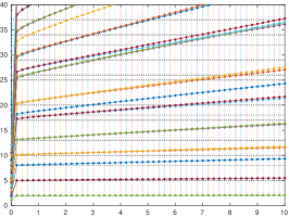
(a) $k=1$, $\beta=0$, $\alpha\in[0,10]$

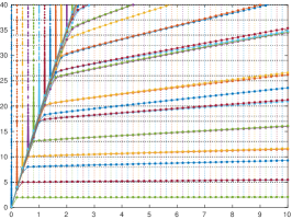
(b) $k=1$, $\beta=1$, $\alpha\in[0,10]$

(c) $k=1$, $\beta=5$, $\alpha\in[0,10]$

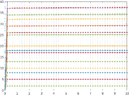
(d) $k=2$, $\beta=0$, $\alpha=[0,10]$

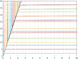
(e) $k=2$, $\beta=1$, $\alpha=[0,10]$

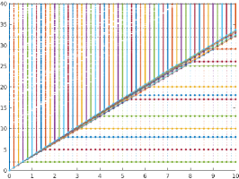
(f) $k=2$, $\beta=5$, $\alpha=[0,10]$

(g) $k=3$, $\beta=0$, $\alpha=[0,10]$

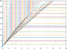
(h) $k=3$, $\beta=1$, $\alpha=[0,10]$

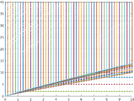
(i) $k=3$, $\beta=5$, $\alpha=[0,10]$

Figure 6: Eigenvalues versus $\alpha$ for different values of $k$ and $\beta$

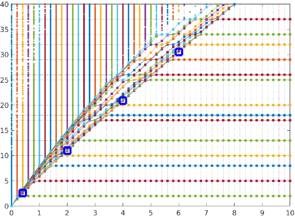
Figure 7: Same plot as in Fig. 6(h) with four marked (spurious) eigenvalues

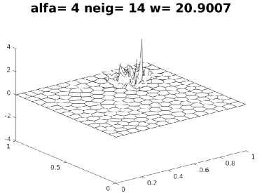
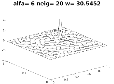
Figure 8: Eigenfunctions corresponding to the eigenvalues marked in Fig. 7

More reliable results seem to be obtained for large $k$ and small $\beta$. Actually, the limit case of $\beta=0$ appears to be the safest choice. This is in agreement with the claim of [5] where the authors remark that “even the value $\sigma_{E}=0$ yields very accurate results, in spite of the fact that for such a value of the parameter the stability estimate and hence most of the proofs of the theoretical results do not hold” (note that $\sigma_{E}=0$ in [5] has the same meaning as $\beta$ in our paper). It is interesting to observe that the analysis of [15], summarized in 1, covers the case $\beta=0$ as well. On the other hand $\beta=0$ may produce a singular matrix $\mathsf{B}$ and this could be not convenient from the computational point of view.

In order to better understand the behavior of the eigenvalues reported in Fig. 6(h), we highlight in Fig. 7 four eigenvalues that are apparently aligned along an oblique line. The corresponding eigenfunctions are reported in Fig. 8. The four eigenfunctions look similar, so that the analogy with Fig. 1 (left) is even more evident.

We conclude this discussion with an example where, for a given value of $\alpha$, a good eigenvalue (i.e., an eigenvalue corresponding to a correct approximation) is crossing a spurious one (i.e., an eigenvalue belonging to an oblique line). In this case it may happen that the two eigenfunctions mix together, thus yielding to an even more complicated situation. This behavior is reported in Fig. 9, where a region of the plot shown in Fig. 6(h) is blown-up close to an intersection point: actually three eigenvalues (a spurious one and two corresponding to good ones) are clustered at the marked intersection points.

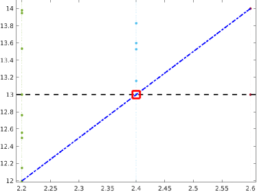
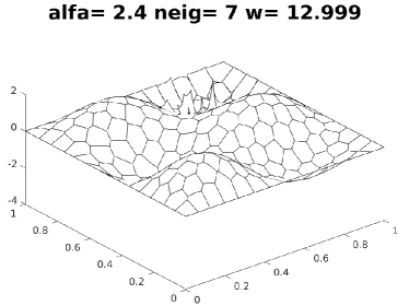
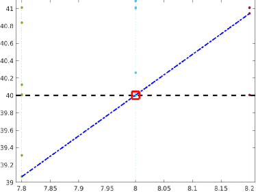
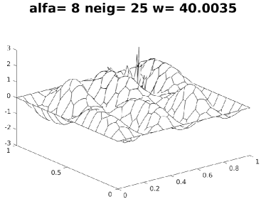
Figure 9: Intersections of good and spurious eigenvalues

Figure 10 shows the computed eigenvalues smaller that $40$ when $\beta$ varies from $0$ to $5$ and for a fixed value of $\alpha$. As in Fig. 5 and in analogy with Fig. 6, the rows correspond to the degree $k$ of polynomials, while the columns refer to different values of $\alpha$. The dotted horizontal lines represent the exact eigenvalues. The lines with different colors in each picture follow the $n$-th eigenvalue for $n=1,\dots,30$. It turns out that all lines are originating from curves that look like hyperbolas when $\beta$ is large. Following each of these hyperbolas from $\beta=+\infty$ backwards, it happens that when the hyperbola meets a correct approximation of an eigenvalue of the continuous problem, it deviates from its trajectory and becomes a (almost horizontal) straight line. In the case $k=1$, we see that the higher eigenvalues are computed with decreasing accuracy as $\beta$ approaches $0$.

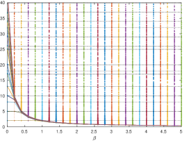
(a) $k=1$, $\alpha=0.1$, $\beta\in[0,5]$

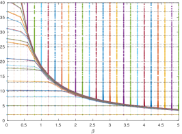
(b) $k=1$, $\alpha=1$, $\beta\in[0,5]$

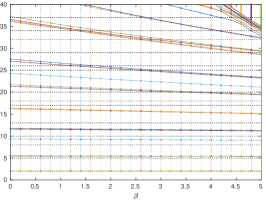
(c) $k=1$, $\alpha=10$, $\beta\in[0,5]$

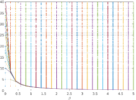
(d) $k=2$, $\alpha=0.1$, $\beta=[0,5]$

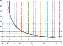
(e) $k=2$, $\alpha=1$, $\beta=[0,5]$

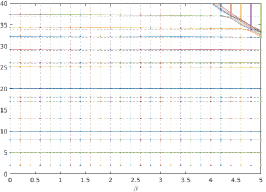
(f) $k=2$, $\alpha=10$, $\beta=[0,5]$

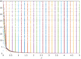
(g) $k=3$, $\alpha=0.1$, $\beta=[0,5]$

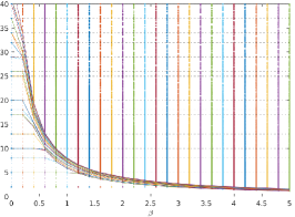
(h) $k=3$, $\alpha=1$, $\beta=[0,5]$

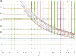
(i) $k=3$, $\alpha=10$, $\beta=[0,5]$

Figure 10: Eigenvalues versus $\beta$ for different values of $k$ and $\alpha$

We recognize in these pictures the situation presented in Section 2.2, corresponding to the behavior of the eigenvalues when the parameter $\beta$ in matrix $\mathsf{B}$ varies. In this test, the kernel of matrix $\mathsf{B}_{1}$ is not empty only for $k=3$. Nevertheless, we can see that when $\beta$ approaches $0$, there are several eigenvalues going to $\infty$. On the other side, for greater values of $\beta$ we obtain several spurious eigenvalues. The range of $\beta$, which gives eigenvalues close to the exact ones, clearly depends on $k$ and $\alpha$.

Figure 11 displays, in separate pictures, the first four eigenvalues, with $k=1$, $\alpha=10$, different values of $h$, and $0\leq\beta\leq 400$. Taking into account that the routine eig sorts the eigenvalues in ascending order, the four pictures display, in lexicographical order, the first, second, third and fourth computed eigenvalues. In each subplot, each line refers to a particular mesh. We can see that the eigenvalues computed with the finest mesh seem to be insensitive with respect to the value of $\beta$. On the opposite side the coarsest mesh gives approximations of the correct values only when $\beta$ is very small and, furthermore, the accuracy is rather low. For each eigenvalue and each fixed mesh we recognize a critical value of the parameter such that greater values of $\beta$ produce spurious eigenvalues. The behavior of these eigenvalues clearly reproduces that of the eigenvalues in Fig. 1 (right) referring to Case 2. The results are plotted with a different perspective depending on the fact that the results now depend also on the computational mesh. The right bottom plot of Fig. 11 highlights a phenomenon which already appears in Fig. 10(i). Indeed, we see that the red line corresponding to the fourth computed eigenvalue for $N=400$ lies along an hyperbola until $\beta=65$ where it reaches the value $5$ associated with second and third exact eigenvalues. Between $\beta=65$ and $\beta=55$ the red line remains close to $5$, then decreasing $\beta$ it follows a different hyperbola until it reaches the expected value for $\beta=35$.

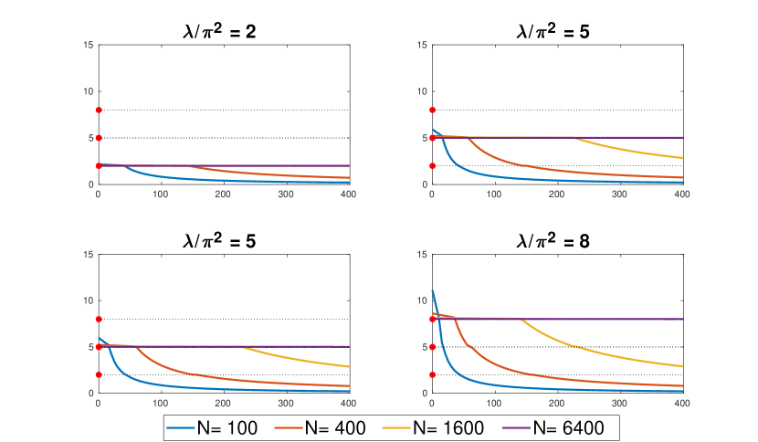
Figure 11: First four eigenvalues

Conclusions

In this paper we have discussed how numerically computed eigenvalues can depend on discretization parameters. Section 2 shows the dependence on $\alpha$ and $\beta$ of the eigenvalues of (1) when $\mathsf{A}$ and $\mathsf{B}$ have the forms (3) and (4), respectively. In Section 3 we have studied the behavior of the eigenvalues of the Laplace operator computed with the Virtual Element Method. The presence of two parameters resembles the abstract setting of Section 2; even if assumptions satisfied by the VEM matrices are more complicated than the ones previously discussed, the numerical results are pretty much in agreement. The present work opens the question of a viable choice of the parameters for eigenvalue computations when the discretization scheme depends on a suitable tuning of them (such as in the case of VEM).

References

- [1] B. Ahmad, A. Alsaedi, F. Brezzi, L. D. Marini, and A. Russo, Equivalent projectors for virtual element methods, Comput. Math. Appl., 66 (2013), pp. 376–391, https://doi.org/10.1016/j.camwa.2013.05.015, https://doi.org/10.1016/j.camwa.2013.05.015.
- [2] S. Badia and R. Codina, A nodal-based finite element approximation of the Maxwell problem suitable for singular solutions, SIAM J. Numer. Anal., 50 (2012), pp. 398–417, https://doi.org/10.1137/110835360.
- [3] L. Beirão da Veiga, F. Brezzi, A. Cangiani, G. Manzini, L. D. Marini, and A. Russo, Basic principles of virtual element methods, Math. Models Methods Appl. Sci., 23 (2013), pp. 199–214, https://doi.org/10.1142/S0218202512500492.
- [4] L. Beirão da Veiga, C. Lovadina, and A. Russo, Stability analysis for the virtual element method, Math. Models Methods Appl. Sci., 27 (2017), pp. 2557–2594, https://doi.org/10.1142/S021820251750052X.
- [5] L. Beirão da Veiga, D. Mora, G. Rivera, and R. Rodríguez, A virtual element method for the acoustic vibration problem, Numer. Math., 136 (2017), pp. 725–763, https://doi.org/10.1007/s00211-016-0855-5.
- [6] D. Boffi, M. Farina, and L. Gastaldi, On the approximation of Maxwell’s eigenproblem in general 2D domains, Computers & Structures, 79 (2001), pp. 1089 – 1096.
- [7] A. Bonito and J.-L. Guermond, Approximation of the eigenvalue problem for the time harmonic Maxwell system by continuous Lagrange finite elements, Math. Comp., 80 (2011), pp. 1887–1910, https://doi.org/10.1090/S0025-5718-2011-02464-6.
- [8] A. Buffa and I. Perugia, Discontinuous Galerkin approximation of the Maxwell eigenproblem, SIAM J. Numer. Anal., 44 (2006), pp. 2198–2226, https://doi.org/10.1137/050636887.
- [9] A. Cangiani, G. Manzini, A. Russo, and N. Sukumar, Hourglass stabilization and the virtual element method, Internat. J. Numer. Methods Engrg., 102 (2015), pp. 404–436, https://doi.org/10.1002/nme.4854.
- [10] M. Costabel and M. Dauge, Maxwell and Lamé eigenvalues on polyhedra, Math. Methods Appl. Sci., 22 (1999), pp. 243–258.
- [11] M. Costabel and M. Dauge, Weighted regularization of Maxwell equations in polyhedral domains. A rehabilitation of nodal finite elements, Numer. Math., 93 (2002), pp. 239–277, https://doi.org/10.1007/s002110100388.
- [12] M. Costabel and M. Dauge, Computation of resonance frequencies for Maxwell equations in non-smooth domains, in Topics in computational wave propagation, vol. 31 of Lect. Notes Comput. Sci. Eng., Springer, Berlin, 2003, pp. 125–161, https://doi.org/10.1007/978-3-642-55483-4_4.
- [13] L. Elsner and J. G. Sun, Perturbation theorems for the generalized eigenvalue problem, Linear Algebra Appl., 48 (1982), pp. 341–357, https://doi.org/10.1016/0024-3795(82)90120-3.
- [14] F. Gardini, G. Manzini, and G. Vacca, The nonconforming virtual element method for eigenvalue problems, ESAIM Math. Model. Numer. Anal., 53 (2019), pp. 749–774, https://doi.org/10.1051/m2an/2018074.
- [15] F. Gardini and G. Vacca, Virtual element method for second-order elliptic eigenvalue problems, IMA J. Numer. Anal., 38 (2018), pp. 2026–2054, https://doi.org/10.1093/imanum/drx063.
- [16] G. H. Golub and C. F. Van Loan, Matrix computations, Johns Hopkins Studies in the Mathematical Sciences, Johns Hopkins University Press, Baltimore, MD, fourth ed., 2013.
- [17] A. Greenbaum, R. cang Li, and M. L. Overton, First-order perturbation theory for eigenvalues and eigenvectors, 2019, https://arxiv.org/abs/1903.00785.
- [18] R.-C. Li and G. W. Stewart, A new relative perturbation theorem for singular subspaces, Linear Algebra Appl., 313 (2000), pp. 41–51, https://doi.org/10.1016/S0024-3795(00)00074-4.
- [19] D. Mora, G. Rivera, and R. Rodríguez, A virtual element method for the Steklov eigenvalue problem, Math. Models Methods Appl. Sci., 25 (2015), pp. 1421–1445, https://doi.org/10.1142/S0218202515500372.
- [20] D. Mora, G. Rivera, and I. Velásquez, A virtual element method for the vibration problem of Kirchhoff plates, ESAIM Math. Model. Numer. Anal., 52 (2018), pp. 1437–1456, https://doi.org/10.1051/m2an/2017041.
- [21] D. Mora and I. Velásquez, A virtual element method for the transmission eigenvalue problem, Math. Models Methods Appl. Sci., 28 (2018), pp. 2803–2831, https://doi.org/10.1142/S0218202518500616.
- [22] O.Čertík, F. Gardini, G. Manzini, L. Mascotto, and G. Vacca, The p- and hp-versions of the virtual element method for elliptic eigenvalue problems, Computers & Mathematics with Applications, (2019), https://doi.org/https://doi.org/10.1016/j.camwa.2019.10.018.
- [23] D. Sármány, F. Izsák, and J. J. W. van der Vegt, Optimal penalty parameters for symmetric discontinuous Galerkin discretisations of the time-harmonic Maxwell equations, J. Sci. Comput., 44 (2010), pp. 219–254, https://doi.org/10.1007/s10915-010-9366-1.
- [24] B. Simon, Fifty years of eigenvalue perturbation theory, Bull. Amer. Math. Soc. (N.S.), 24 (1991), pp. 303–319, https://doi.org/10.1090/S0273-0979-1991-16020-9.
- [25] G. W. Stewart and J. G. Sun, Matrix perturbation theory, Computer Science and Scientific Computing, Academic Press, Inc., Boston, MA, 1990.
- [26] T. Warburton and M. Embree, The role of the penalty in the local discontinuous Galerkin method for Maxwell’s eigenvalue problem, Comput. Methods Appl. Mech. Engrg., 195 (2006), pp. 3205–3223, https://doi.org/10.1016/j.cma.2005.06.011.