An extended 3-3-1 model with two scalar triplets and linear seesaw mechanism

Abstract

Low energy linear seesaw mechanism responsible for the generation of the tiny active neutrino masses, is implemented in the extended 3-3-1 model with two scalar triplets and right handed Majorana neutrinos where the gauge symmetry is supplemented by the $A_{4}$ flavor discrete group and other auxiliary cyclic symmetries, whose spontaneous breaking produces the observed pattern of SM charged fermion masses and fermionic mixing parameters. Our model is consistent with the low energy SM fermion flavor data as well as with the constraints arising from meson oscillations. Some phenomenological aspects such as the $Z^{\prime}$ production at proton-proton collider and the lepton flavor violating decay of the SM-like Higgs boson are discussed. The scalar potential of the model is analyzed in detail and the SM-like Higgs boson is identified.

Keywords: Extensions of electroweak gauge sector, Extensions of electroweak Higgs sector, Electroweak radiative corrections, Neutrino mass and mixing

I Introduction

It is well-known, that there are various experimental and theoretical observations indicating that the Standard Model (SM) must be extended. Among the theories beyond the SM, the models based on the gauge group $SU(3)_{C}\times SU(3)_{L}\times U(1)_{X}$ (called 3-3-1 for short) [1, 2, 3, 4, 5, 6, 7, 8, 9, 10, 11, 12, 13, 14, 15, 16, 17, 18, 19, 20, 21, 22, 23, 24, 25, 26, 27, 28, 29, 30, 31, 32, 33, 34, 35, 36, 37, 38, 39, 40, 41, 42, 43, 44, 45, 46, 47, 48, 49] have some intriguing features allowing them to explain the number of SM fermion families, the electric charge quantization [50, 51], etc. In the ordinary 3-3-1 models, the Higgs sector contains at least three scalar triplets significantly extending their scalar spectrum. Attempts aimed to reduce the Higgs sector of the 3-3-1 models have been undertaken in the literature. A model with the parameter $\beta=-\frac{1}{\sqrt{3}}$, defined in (3) and characterizing the embedding of the electric charge generator into $SU(3)_{L}$, has been proposed in Refs. [52, 53, 54, 55, 56, 57, 47]. Due to its restricted scalar sector it is called the economical 3-3-1 model. However, this and other similar versions of the 3-3-1 model with the reduced scalar content failed to reproduce the neutrino oscillation data. In a view of these difficulties a 3-3-1 model with $\beta=\frac{1}{\sqrt{3}}$ and containing just two Higgs triplets has been studied in Ref. [41]. In this model the masses of light active neutrinos and charged fermions are generated via Type-I Seesaw and the Universal Seesaw mechanisms, respectively. However, the fermion mixing was not addressed in Ref. [41].

In the present paper we propose a multiscalar singlet extension of the 3-3-1 model with two $SU(3)_{L}$ scalar triplets and three right handed Majorana neutrinos. The gauge group of the model is extended with the $A_{4}$ group and some other cyclic symmetries in order to implement the linear seesaw mechanism responsible for the tiny masses of the active neutrinos. A well-known advantage of the linear seesaw mechanism [58, 59, 60, 61, 62, 63, 64, 65, 66, 62, 67] is its testability at the LHC, since it implies sterile neutrinos with TeV-scale masses. Our model also successfully addresses the observed pattern of the SM fermion masses and mixings, as a result of the spontaneous breaking of the above mentioned discrete group factors, in an analogous way to the Froggat-Nielsen mechanism [68], which has also been implemented in 3-3-1 models through the breaking of a $U(1)$ global symmetry in Refs. [69, 70, 71]. We choose $A_{4}$ as the smallest discrete group having one three-dimensional and three distinct one-dimensional irreducible representations allowing us to naturally accommodate the three families of the SM. The $A_{4}$ discrete flavour group has received a lot interest by the model building community due to its remarkable ability to elucidate the observed pattern of SM fermion masses and mixing angles [72, 73, 74, 75, 76, 77, 78, 79, 80, 81, 82, 83, 84, 85, 86, 87, 88, 89, 90, 91, 92, 93, 94, 95, 96, 31, 97, 98, 39, 99, 100, 101, 102, 103, 104, 105, 106, 107, 62, 108, 109, 110, 111, 112].

Comparing our model with others, we note, in particular, that our $U(1)_{X}$-charge assignments of the left handed quark $SU(3)_{L}$-triplets are different from those in the model of Ref. [41]. Due to this difference we have two exotic down type quarks and one exotic up type quarks whereas in the model of Ref. [41] there are two exotic up type quarks and one exotic down type quark. In addition, whereas in our model the small masses for the active neutrinos are produced from a linear seesaw mechanism, in the model of Ref. [41] they are generated from a type-I seesaw mechanism. In Ref. [41], the extra fermion lying in the bottom of the lepton triplet is a charged lepton instead of the right-handed neutrino, which is the field of the third component of $SU(3)_{L}$ leptonic triplet in our model.

Let us also note that our model is more predictive and significantly more economical in its particle content than the 3-3-1 model with $T^{\prime}$ and $S_{4}$ symmetries proposed in [47, 48]. For instance, whereas the scalar sector of the $T^{\prime}$ flavored 3-3-1 model [47] includes two $SU(3)_{L}$ scalar triplets and $23$ gauge singlet scalar fields, the present model has two $SU(3)_{L}$ scalar triplets and $16$ $SU(3)_{L}$ singlet scalar fields. As for the scalar sector of the 3-3-1 model with $S_{4}$ family symmetry [48], it contains 3 $SU(3)_{L}$ scalar triplets and $32$ gauge singlet scalar fields, which is much larger than the number of scalar degrees of freedom of our model. Let us note, that in the proposed model some quarks and scalar fields carry lepton number, which leads to flavor lepton number violating decay modes of the SM-like Higgs boson. In what follows we will study this phenomenological aspect of our model as well as the production of the extra heavy neutral gauge boson $Z^{\prime}$ and its detection in the dimuon channel at the LHC. However, the emphasis will be made on studying the SM fermion masses and mixings.

The paper is organized as follows. In Sect. II we introduce the model setup. Sects. III and V are devoted to the model predictions for the masses and mixings in the quark and lepton sectors, respectively. Sect. IV discusses the constraints on the $Z^{\prime}$ mass arising from meson oscillations. In Sect. VII the lepton flavor violating (LFV) decays of the charged leptons and the Higgs boson are considered. In Sect. VIII we summarize our results and discuss their further implications. In Appendix A we present the discrete group $A_{4}$ group characters. A detailed description of the Higgs sector of the model is given in Appendix B. The analytic formulas for one-loop contributions to the LFV decay amplitudes of the SM-like Higgs boson are collected in Appendix C. The couplings of neutral gauge bosons $Z$ and $Z^{\prime}$ to fermions are listed in appendix D.

II The model

We propose a 3-3-1 model where the scalar sector is composed of two $SU(3)_{L}$ scalar triplets and seven $SU(3)_{L}$ scalar singlets and the fermion sector corresponds to the one of the 3-3-1 models with three right handed Majorana neutrinos. In our model the $SU(3)_{C}\times SU(3)_{L}\times U(1)_{X}$  gauge symmetry is supplemented with the $A_{4}\times Z_{8}\times Z_{14}\times Z_{22}$ discrete group, so that the full symmetry $\mathcal{G}$ exhibits the following three-step spontaneous breaking:

$$\mathcal{G}=SU(3)_{C}\times SU(3)_{L}\times U(1)_{X}\times A_{4}\times Z_{8}\times Z_{14}\times Z_{22}$$ (1)

$$\hskip 99.58464pt\Downarrow\Lambda_{int}$$

$$\hskip 42.67912ptSU(3)_{C}\times SU(3)_{L}\times U(1)_{X}$$

$$\hskip 99.58464pt\Downarrow v_{\chi}$$

$$\hskip 42.67912ptSU(3)_{C}\otimes SU(2)_{L}\times U(1)_{Y}$$

$$\hskip 99.58464pt\Downarrow v_{\eta}$$

$$\hskip 65.44133ptSU(3)_{C}\otimes U(1)_{Q}$$

where the different symmetry breaking scales satisfy the following hierarchy

$$v_{\eta}=v=246\mbox{GeV}\ll v_{\chi}\sim\mathcal{O}(10)\mbox{TeV}.$$ (2)

In the 3-3-1 model under consideration, the electric charge is defined in terms of the $SU(3)$ generators and the identity by:

$$Q=T_{3}+\beta T_{8}+X=T_{3}-\frac{1}{\sqrt{3}}T_{8}+X,$$ (3)

where we have chosen $\beta=-\frac{1}{\sqrt{3}}$ (without non-SM electric charges), which implies that bottom component of the lepton $SU(3)_{L}$-triplet is a neutral field $\nu_{R}^{C}$ thus allowing to build the Dirac matrix with the usual field $\nu_{L}$ in the top component of the lepton triplet. Adding gauge singlet right-handed Majorana neutrinos $N_{iR}$ $(i=1,2,3)$ will allow us to implement a low scale seesaw mechanism, which could be inverse or linear, to generate the masses for the light active neutrinos. These low scale seesaw mechanisms offer attractive explanations for the smallest of neutrino masses because they can be tested at the LHC via the production and decay of sterile neutrinos. It is worth mentioning that the sterile neutrinos can be produced at the LHC in association with a SM charged lepton and in pairs, via quark-antiquark annihilation mediated by a $W$ and heavy $W^{\prime}$ and $Z^{\prime}$ gauge bosons, respectively. In our model the sterile neutrinos have the following two body decay modes: $N^{\pm}_{a}\rightarrow l^{\pm}_{i}W^{\mp}$ and $N^{\pm}_{a}\rightarrow\nu_{i}Z$ (where $a,i=1,2,3$), which are suppressed by the small active-sterile neutrino mixing angle. Furthermore the heavy sterile neutrinos $N^{\pm}_{a}$ can decay via off-shell gauge bosons via the following modes: $N^{\pm}_{a}\rightarrow l^{+}_{i}l^{-}_{j}\nu_{k}$, $N^{\pm}_{a}\rightarrow l^{-}_{i}u_{j}\bar{d}_{k}$, $N^{\pm}_{a}\rightarrow b\bar{b}\nu_{k}$ (where $a,i,j,k=1,2,3$ are flavour indices). Thus, the heavy sterile neutrinos can be detected at the LHC from the observation of an excess of events with respect to the SM background in a final state composed of a pair of opposite sign charged leptons plus two jets. Studies of inverse seesaw neutrino signatures at colliders as well as the production of heavy neutrinos at the LHC are carried out in [113, 114, 115, 116, 117, 118, 119, 120, 121, 122, 123, 124, 125, 126, 127, 128, 129]. A detailed study of the sterile neutrino production at the LHC and the sterile neutrino modes goes beyond the scope of this work and will be done elsewhere.

The cancellation of chiral anomalies implies that the number of triplets equals that of antitriplets, so that quarks are unified in the following $SU(3)_{C}\times SU(3)_{L}\times U(1)_{X}$ left- and right-handed representations [2, 7, 130, 9]:

$$Q_{nL} =\left(D_{n}\,,-U_{n}\,,J_{n}\,\right)^{T}_{L}\sim(3,3^{\ast},0),\hskip 28.45274ptQ_{3L}=\left(U_{3}\,,D_{3}\,,\,T\right)^{T}_{L}\sim\left(3,3,\frac{1}{3}\right),\hskip 28.45274ptn=1,2,$$

$$D_{iR} \sim\left(3,1,-\frac{1}{3}\right),\hskip 28.45274ptU_{iR}\sim\left(3,1,\frac{2}{3}\right),\hskip 28.45274ptJ_{nR}\sim\left(3,1,-\frac{1}{3}\right),\hskip 28.45274ptT_{R}\sim\left(3,1,\frac{2}{3}\right),\quad i=1,2,3\,.$$

Furthermore, the requirement of chiral anomaly cancellation constrains the leptons to the following $SU(3)_{C}\times SU(3)_{L}\times U(1)_{X}$ left- and right-handed representations [2, 7, 130]:

$$L_{iL}=\left(\nu_{i}\,,e_{i}\,,\nu_{i}^{c}\right)^{T}_{L}\sim\left(1,3,-\frac{1}{3}\right),\hskip 28.45274pte_{iR}\sim(1,1,-1),\hskip 28.45274pti=1,2,3,$$ (4)

In the present model the fermion sector is extended by introducing three right handed Majorana neutrinos, singlets under the 3-3-1 group, so that they have the following $SU(3)_{C}\times SU(3)_{L}\times U(1)_{X}$ assignments:

$$N_{iR}\sim(1,1,0),\hskip 28.45274pti=1,2,3.$$

Note that in the Ref.[41], where $\beta=+\frac{1}{\sqrt{3}}$, the third component of lepton triplet is an extra charged leptons.

We assign the scalar fields to the following $SU(3)_{C}\times SU(3)_{L}\times U(1)_{X}$ representations:

$$\chi = \begin{pmatrix}\chi_{1}^{0}\\ \chi_{2}^{-}\\ \frac{1}{\sqrt{2}}(v_{\chi}+\xi_{\chi}\pm i\zeta_{\chi})\end{pmatrix}\sim\left(1,3,-\frac{1}{3}\right),\hskip 28.45274pt\eta=\begin{pmatrix}\frac{1}{\sqrt{2}}(v_{\eta}+\xi_{\eta}\pm i\zeta_{\eta})\\ \eta_{2}^{-}\\ \eta_{3}^{0}\end{pmatrix}\sim\left(1,3,-\frac{1}{3}\right),$$ (5)

$$\sigma \sim (1,1,0),\hskip 28.45274pt\hskip 28.45274pt\xi_{i}\sim(1,1,0),\hskip 28.45274pt\hskip 28.45274pt\zeta_{i}\sim(1,1,0),\hskip 28.45274pt\hskip 28.45274pti=1,2,3.$$

$$\rho_{i} \sim (1,1,0),\hskip 28.45274pt\hskip 28.45274pt\varphi_{i}\sim(1,1,0),\hskip 28.45274pt\hskip 28.45274pt\phi_{i}\sim(1,1,0).$$

Here $v_{\chi},v_{\eta}$ are the vev’s setting symmetry breaking scales in (1), (2).
The scalar assignments under the $A_{4}\times Z_{8}\times Z_{14}\times Z_{22}$ discrete group are summarized in Table 1.

In our model this discrete global symmetry group is not only spontaneously broken, it is softly broken as well. Let us note that the gauge singlet scalars of our models are complex, which implies that in order to provide masses for the CP odd parts of these scalars, one has to include $A_{4}\times Z_{8}\times Z_{14}\times Z_{22}$ soft breaking bilinear terms in the scalar potential involving a pair of these scalar singlets. These soft breaking scalar mass terms will also be useful for resolving the domain wall problem, arising from the spontaneous breaking the global discrete symmetries.

	$\chi$	$\eta$	$\sigma$	$\xi$	$\zeta$	$\rho$	$\phi$	$\varphi$
$A_{4}$	$\mathbf{1}$	$\mathbf{1}$	$\mathbf{1}^{\prime}$	$\mathbf{3}$	$\mathbf{3}$	$\mathbf{3}$	$\mathbf{3}$	$\mathbf{3}$
$Z_{8}$	$0$	$-1$	$0$	$1$	$-7$	$-1$	$-1$	$4$
$Z_{14}$	$0$	$-1$	$0$	$1$	$-7$	$1$	$1$	$1$
$Z_{22}$	$0$	$-2$	$-1$	$2$	$-1$	$2$	$2$	$2$

Table 1: Scalar assignments under $A_{4}\times Z_{8}\times Z_{14}\times Z_{22}$.

In Appendix B we present more details about the scalar sector of our model.

In what follows we briefly describe the gauge sector of our model. Here we have 8 electroweak $SU(3)_{L}$ gauge bosons, $W_{a\mu}$, and a $U(1)_{X}$ gauge boson, $\widetilde{B}_{\mu}$.

From the scalar kinetic term one finds the interactions:

$$(D^{\mu}H)^{\dagger}D_{\mu}H\supset\partial^{\mu}R_{H}^{\dagger}P_{\mu}I_{H}-R^{\dagger}P^{\mu}\partial_{\mu}I_{H}\,{\color[rgb]{0,0,1},}\,H=\eta,\chi,$$ (6)

The covariant derivative is defined as

$$D_{\mu}=\partial_{\mu}-iT_{a}W_{a\mu}-ig_{X}T_{9}X\widetilde{B}_{\mu}=\partial_{\mu}-i\Pi_{\mu}$$ (7)

with:

$$\Pi_{\mu}=\frac{g}{2}\left(\begin{array}[]{ccc}W_{3\mu}+\frac{1}{\sqrt{3}}W_{8\mu}+t\sqrt{\frac{2}{3}}X\widetilde{B}_{\mu}&\sqrt{2}W_{\mu}^{+}&\sqrt{2}X_{\mu}^{q_{1}}\\ \sqrt{2}W_{\mu}^{-}&-W_{3\mu}+\frac{1}{\sqrt{3}}W_{8\mu}+t\sqrt{\frac{2}{3}}X\widetilde{B}_{\mu}&\sqrt{2}Y_{\mu}^{q_{2}}\\ \sqrt{2}X_{\mu}^{-q_{1}}&\sqrt{2}Y_{\mu}^{-q_{2}}&-\frac{2}{\sqrt{3}}W_{8\mu}+t\sqrt{\frac{2}{3}}X\widetilde{B}_{\mu}\end{array}\right),\hskip 28.45274ptt=\frac{g_{X}}{g}$$

where

$$W_{\mu}^{\pm}=\frac{1}{\sqrt{2}}\left(W_{1}\mp iW_{2}\right),\hskip 28.45274ptX_{\mu}^{q_{1}}=\frac{1}{\sqrt{2}}\left(W_{4}-iW_{5}\right),\hskip 28.45274ptY_{\mu}^{q_{2}}=\frac{1}{\sqrt{2}}\left(W_{6}-iW_{7}\right).$$ (8)

Then, in the gauge sector we have three electrically neutral $q=0$ gauge fields, which combine to form the photon and $Z$, $Z^{\prime}$-bosons, two fields $W^{\pm}$ with $q=\pm 1$ and $X_{\mu}^{q_{1}}$, $Y_{\mu}^{q_{2}}$ with electrical charges

$$q_{1} = \frac{1}{2}+\frac{\sqrt{3}\beta}{2},\hskip 28.45274ptq_{2}=-\frac{1}{2}+\frac{\sqrt{3}\beta}{2}.$$ (9)

Physical neutral gauge bosons for $\beta=-\frac{1}{\sqrt{3}}$ are given by:

$$A_{\mu} = c_{W}\left(-\sqrt{\frac{1}{3}}t_{W}W_{8\mu}+\frac{\sqrt{3-4s_{W}^{2}}}{\sqrt{3}c_{W}}\widetilde{B}_{\mu}\right)+s_{W}W_{3\mu},$$

$$Z_{\mu} = c_{W}W_{3\mu}-s_{W}\left(-\sqrt{\frac{1}{3}}t_{W}W_{8\mu}+\frac{\sqrt{3-4s_{W}^{2}}}{\sqrt{3}c_{W}}\widetilde{B}_{\mu}\right),$$

$$Z_{\mu}^{\prime} = -\sqrt{\frac{1}{3}}t_{W}\widetilde{B}_{\mu}-\frac{\sqrt{3-4s_{W}^{2}}}{\sqrt{3}c_{W}}W_{8\mu}$$

$$X_{\mu}^{0} = \frac{1}{\sqrt{2}}\left(W_{\mu 4}-iW_{\mu 5}\right),\hskip 28.45274pt\bar{X}_{\mu}^{0}=\frac{1}{\sqrt{2}}\left(W_{\mu 4}+iW_{\mu 5}\right)$$ (10)

where $c_{W}=\cos\theta_{W}$, $s_{W}=\cos\theta_{W}$ and $t_{W}=\tan\theta_{W}$, being $\theta_{W}$ the weak mixing angle. In addition, for $\beta=-\frac{1}{\sqrt{3}}$, which corresponds to our model, we find the relations:

$$\widetilde{B}_{\mu}=-\sqrt{\frac{1}{3}}t_{W}Z_{\mu}^{\prime}+\frac{\sqrt{3-4s_{W}^{2}}}{\sqrt{3}c_{W}}\left(c_{W}A_{\mu}-s_{W}Z_{\mu}\right),\hskip 28.45274ptW_{8\mu}=-\sqrt{\frac{1}{3}}t_{W}\left(c_{W}A_{\mu}-s_{W}Z_{\mu}\right)-\frac{\sqrt{3-4s_{W}^{2}}}{\sqrt{3}c_{W}}Z_{\mu}^{\prime},$$ (11)

$$t=\frac{g_{X}}{g}=\frac{3\sqrt{2}s_{W}}{\sqrt{3-4s_{W}^{2}}}.$$ (12)

The electrically charged gauge bosons are given by:

$$W_{\mu}^{\pm}=\frac{1}{\sqrt{2}}\left(A_{\mu 1}\mp iA_{\mu 2}\right)\,,\hskip 8.5359ptY_{\mu}^{\pm}=\frac{1}{\sqrt{2}}\left(A_{\mu 6}\pm iA_{\mu 7}\right)\,$$ (13)

where $Y^{\pm}$ and $X^{0}$ are bilepton gauge bosons. With the above-discussed structure of the scalar sector of the model, the massive gauge bosons acquire the following masses [131]:

$$m^{2}_{W}=m^{2}_{Z}c^{2}_{W}=\frac{g^{2}}{4}v_{\eta}^{2}\,,\hskip 8.5359ptM^{2}_{X^{0}}=M^{2}_{\bar{X}^{0}}=\frac{g^{2}}{4}\left(v^{2}_{\chi}+v_{\eta}^{2}\right)\,,\hskip 8.5359ptM^{2}_{Y}=\frac{g^{2}}{4}v_{\chi}^{2}\,\,,\hskip 8.5359ptM^{2}_{Z^{\prime}}\simeq\frac{g^{2}v_{\chi}^{2}}{3-t^{2}_{W}},$$ (14)

where $v_{\eta}=v=246$ GeV. From (14) we find the mass splitting

$$M^{2}_{X^{0}}-M^{2}_{Y}=m^{2}_{W}\,.$$ (15)

In Ref. [132] it was shown that the contributions of the bilepton gauge boson $Y^{\pm},X^{0}$ to the oblique $S$ and $T$ parameters are constrained to be in the ranges $-0.085\lesssim S\lesssim 0.05$, $-0.001\lesssim T\lesssim 0.08$, respectively. In the scenario where the mixing angles between the exotic and the SM quarks are small, which is the the case of our model, the exotic quark contributions to these oblique parameters are very subleading since they are suppressed by the square of the small mixing angles. Consequently, the dominant contributions to the oblique $S$ and $T$ parameters are the ones arising from the bilepton gauge bosons $Y^{\pm}$ and $X^{0}$. Notice that the aforementioned range of values for the $S$ and $T$ parameters allow one to have a region of the model parameter space where the obtained values for these oblique parameters are inside the experimentally allowed region of Ref. [133] enclosed by the ellipses in the $S-T$ plane.

The fermion assignments under the $A_{4}\times Z_{8}\times Z_{14}\times Z_{22}$ discrete group are summarized in Table 2.

	$Q_{1L}$	$Q_{2L}$	$Q_{3L}$	$U_{1R}$	$U_{2R}$	$U_{3R}$	$T_{R}$	$D_{1R}$	$D_{2R}$	$D_{3R}$	$J_{1R}$	$J_{2R}$	$L_{L}$	$N_{R}$	$e_{1R}$	$e_{2R}$	$e_{3R}$
$A_{4}$	$\mathbf{1}^{\prime\prime}$	$\mathbf{1}^{\prime}$	$\mathbf{1}$	$\mathbf{1}^{\prime\prime}$	$\mathbf{1}^{\prime}$	$\mathbf{1}$	$\mathbf{1}$	$\mathbf{1}^{\prime}$	$\mathbf{1}^{\prime\prime}$	$\mathbf{1}^{\prime\prime}$	$\mathbf{1}^{\prime\prime}$	$\mathbf{1}^{\prime}$	$\mathbf{3}$	$\mathbf{3}$	$\mathbf{1}$	$\mathbf{1}^{\prime}$	$\mathbf{1}$
$Z_{8}$	$0$	$0$	$0$	$-3$	$-1$	$1$	$0$	$2$	$4$	$-1$	$0$	$0$	$0$	$0$	$0$	$3$	$0$
$Z_{14}$	$0$	$0$	$0$	$5$	$-1$	$1$	$0$	$2$	$4$	$-1$	$0$	$0$	$-4$	$-4$	$-6$	$-6$	$-6$
$Z_{22}$	$-5$	$-4$	$0$	$-8$	$-6$	$2$	$0$	$-14$	$-9$	$-1$	$-5$	$-4$	$-7$	$-8$	$-5$	$-9$	$-11$

Table 2: Fermion assignments under $A_{4}\times Z_{8}\times Z_{14}\times Z_{22}$.

We assume the following VEV pattern for the $A_{4}$ triplet SM singlet scalars $\xi$, $\zeta$, $\rho$, $\varphi$ and $\phi$:

$$\left\langle\xi\right\rangle = \frac{v_{\xi}}{\sqrt{3}}(1,1,1),\hskip 28.45274pt\left\langle\zeta\right\rangle=\frac{v_{\zeta}}{\sqrt{2}}(1,0,1),\hskip 28.45274pt\left\langle\rho\right\rangle=\frac{v_{\rho}}{\sqrt{3}}(1,1,1),$$

$$\left\langle\varphi\right\rangle = \frac{v_{\varphi}}{\sqrt{3}}\left(\cos\alpha+e^{i\psi}\sin\alpha,\omega\left(\cos\alpha+\omega e^{i\psi}\sin\alpha\right),\omega^{2}\left(\cos\alpha+\omega^{2}e^{i\psi}\sin\alpha\right)\right),$$ (16)

$$\left\langle\phi\right\rangle = \frac{v_{\phi}}{\sqrt{3}}\left(\cos\alpha-e^{-i\psi}\sin\alpha,\omega^{2}\left(\cos\alpha-\omega^{2}e^{-i\psi}\sin\alpha\right),\omega\left(\cos\alpha-\omega e^{-i\psi}\sin\alpha\right)\right),\hskip 28.45274pt\omega=e^{\frac{2\pi i}{3}},$$

which are consistent with the scalar potential minimization equations for a large region of parameter space, as shown in details in Refs. [134, 39].

With the above particle content, the relevant Yukawa terms for the quark and lepton sectors invariant under the group $\mathcal{G}$ are:

$$-\mathcal{L}_{Y}^{(q)} = y^{(T)}\overline{Q}_{3L}\chi T_{R}+y_{33}^{(U)}\overline{Q}_{3L}\eta U_{3R}$$

$$+y_{22}^{(U)}\varepsilon_{abc}\overline{Q}_{2L}^{a}\eta^{b}\chi^{c}U_{2R}\frac{(\xi\xi)_{\mathbf{\mathbf{1}}}}{\Lambda^{3}}+y_{11}^{(U)}\varepsilon_{abc}\overline{Q}_{1L}^{a}\eta^{b}\chi^{c}U_{1R}\frac{\left(\xi^{3}\zeta\right)_{\mathbf{\mathbf{1}}}}{\Lambda^{5}}$$

$$+y_{1}^{(J)}\overline{Q}_{1L}\chi^{\ast}J_{1R}+y_{2}^{(J)}\overline{Q}_{2L}\chi^{\ast}J_{2R}$$

$$+y_{33}^{(D)}\varepsilon_{abc}\overline{Q}_{3L}^{a}\left(\eta^{\ast}\right)^{b}\left(\chi^{\ast}\right)^{c}D_{3R}\frac{\sigma}{\Lambda^{2}}+y_{22}^{(D)}\overline{Q}_{2L}\eta^{\ast}D_{2R}\frac{\left(\xi^{2}\zeta\right)_{\mathbf{\mathbf{1}}}}{\Lambda^{3}}$$

$$+y_{11}^{(D)}\overline{Q}_{1L}\eta^{\ast}D_{1R}\frac{\left(\xi^{4}\zeta\right)_{\mathbf{\mathbf{1}}}}{\Lambda^{5}}+y_{12}^{(D)}\overline{Q}_{1L}\eta^{\ast}D_{2R}\frac{\left(\xi^{2}\zeta\right)_{\mathbf{\mathbf{1}}}\sigma}{\Lambda^{4}}+y_{13}^{(D)}\overline{Q}_{1L}\eta^{\ast}D_{3R}\frac{\sigma^{6}}{\Lambda^{6}}+y_{23}^{(D)}\overline{Q}_{2L}\eta^{\ast}D_{3R}\frac{\sigma^{5}}{\Lambda^{5}}+H.c,$$

$$-\mathcal{L}_{Y}^{(l)} = y_{1}^{(L)}\varepsilon_{abc}\left(\overline{L}_{L}^{a}\left(\eta^{\ast}\right)^{b}\left(\chi^{\ast}\right)^{c}\rho\right)_{\mathbf{\mathbf{1}}}e_{1R}\frac{\sigma^{6}}{{\Lambda^{8}}}+y_{2}^{(L)}\varepsilon_{abc}\left(\overline{L}_{L}^{a}\left(\eta^{\ast}\right)^{b}\left(\chi^{\ast}\right)^{c}\varphi\right)_{\mathbf{\mathbf{1}}}e_{2R}\frac{\sigma^{2}}{\Lambda^{4}}+\frac{y_{3}^{(L)}}{\Lambda^{2}}\varepsilon_{abc}\left(\overline{L}_{L}^{a}\left(\eta^{\ast}\right)^{b}\left(\chi^{\ast}\right)^{c}\rho\right)_{\mathbf{\mathbf{1}}}e_{3R}$$ (18)

$$+z_{1}^{(L)}\varepsilon_{abc}\left(\overline{L}_{L}^{a}\left(\eta^{\ast}\right)^{b}\left(\chi^{\ast}\right)^{c}\phi\right)_{\mathbf{\mathbf{1}}}e_{1R}\frac{\sigma^{6}}{{\Lambda^{8}}}+\frac{z_{3}^{(L)}}{\Lambda^{2}}\varepsilon_{abc}\left(\overline{L}_{L}^{a}\left(\eta^{\ast}\right)^{b}\left(\chi^{\ast}\right)^{c}\phi\right)_{\mathbf{\mathbf{1}}}e_{3R}$$

$$+y^{(L)}_{\rho}\varepsilon_{abc}\varepsilon_{dec}\left(\overline{L}_{L}^{a}\left(L_{L}^{C}\right)^{b}\right)_{\mathbf{3a}}\eta^{d}\chi^{e}\frac{\zeta\sigma^{11}}{\Lambda^{13}}+y_{1\eta}^{(L)}\left(\overline{L}_{L}\eta N_{R}\right)_{\mathbf{3s}}\frac{\xi\sigma^{\ast}}{\Lambda^{2}}+y_{2\eta}^{(L)}\left(\overline{L}_{L}\eta N_{R}\right)_{\mathbf{3a}}\frac{\xi\sigma^{\ast}}{\Lambda^{2}}$$

$$+y_{\chi}^{(L)}\left(\overline{L}_{L}\chi N_{R}\right)_{\mathbf{1}^{\prime}}\frac{\sigma^{\ast}}{\Lambda}+H.c.\ ,$$

where the dimensionless couplings $y,z$ in Eqs. (II) and (18) are $\mathcal{O}(1)$ parameters. In addition to these terms, the symmetries unavoidably allow the following terms:

$$y^{(T3)}\overline{Q}_{3L}\chi U_{3R}\frac{(\xi^{*2}\xi)_{1}}{\Lambda^{3}},\hskip 56.9055pty^{(3T)}\overline{Q}_{3L}\eta T_{R}\frac{(\xi^{*}\xi^{2})_{1}}{\Lambda^{3}}$$

$$y^{(J_{2}D_{3})}\overline{Q}_{2L}\chi^{\ast}D_{3R}\frac{(\xi^{2}\xi^{*})_{1}\sigma^{5}}{\Lambda^{8}},\hskip 56.9055pty^{(D_{3}J_{2})}\varepsilon_{abc}\overline{Q}_{3L}^{a}\left(\eta^{\ast}\right)^{b}\left(\chi^{\ast}\right)^{c}D_{3R}\frac{(\xi^{\ast 2}\xi)_{1^{\prime}}\sigma^{\ast 4}}{\Lambda^{8}}\,.$$

These terms will generate very small mixing angles of the third generation SM up and down type quarks with the exotic quarks. Such mixing angles are of the order of $\lambda^{5}$ and $\lambda^{11}$ (being $\lambda=0.225$), for the up and down type quarks, respectively, thus allowing us to safely neglect these strongly suppressed corrections, which will not be considered in our analysis. Furthermore, as it will shown in Sect. III, the quark assignments under the different group factors of our model will give rise to SM quark mass textures where the CKM quark mixing angles only arise from the down type quark sector. As indicated by the current low energy quark flavor data encoded in the standard parametrization of the quark mixing matrix, the complex phase responsible for CP violation in the quark sector is associated with the quark mixing angle in the $1$-$3$ plane. Thus, the Yukawa coupling $y_{13}^{(D)}$ in Eq. (II) is required to be complex in order to successfully reproduce the experimental values of the quark mixing angles and CP violating phase.

In a generic scenario the Yukawa couplings are complex. However, not all of them are physical. Some phases can be rotated away by the phase rotation of the quark and lepton fields. The conditions for the rotation away of the Yukawa phases in the quark sector by the redefinition of the phases $\alpha_{f}$ of the quark fields are:

$$\arg\left(y_{33}^{\left(D\right)}\right)-\alpha_{Q_{3L}}+\alpha_{D_{3R}} = 0,\hskip 28.45274pt\arg\left(y_{23}^{\left(D\right)}\right)-\alpha_{Q_{2L}}+\alpha_{D_{3R}}=0,$$

$$\arg\left(y_{13}^{\left(D\right)}\right)-\alpha_{Q_{1L}}+\alpha_{D_{3R}} = 0,\hskip 28.45274pt\arg\left(y_{22}^{\left(D\right)}\right)-\alpha_{Q_{2L}}+\alpha_{D_{2R}}=0,$$

$$\arg\left(y_{12}^{\left(D\right)}\right)-\alpha_{Q_{1L}}+\alpha_{D_{2R}} = 0,\hskip 28.45274pt\arg\left(y_{11}^{\left(D\right)}\right)-\alpha_{Q_{1L}}+\alpha_{D_{1R}}=0,$$

$$\arg\left(y_{1}^{\left(J\right)}\right)-\alpha_{Q_{1L}}+\alpha_{J_{1R}} = 0,\hskip 28.45274pt\arg\left(y_{2}^{\left(J\right)}\right)-\alpha_{Q_{2L}}+\alpha_{J_{2R}}=0,$$

$$\arg\left(y_{11}^{\left(U\right)}\right)-\alpha_{Q_{1L}}+\alpha_{U_{1R}} = 0,\hskip 28.45274pt\arg\left(y_{22}^{\left(U\right)}\right)-\alpha_{Q_{2L}}+\alpha_{U_{2R}}=0,$$

$$\arg\left(y_{33}^{\left(U\right)}\right)-\alpha_{Q_{3L}}+\alpha_{U_{3R}} = 0,\hskip 28.45274pt\arg\left(y^{\left(T\right)}\right)-\alpha_{Q_{3L}}+\alpha_{T_{R}}=0,$$ (19)

Consequently all the Yukawa phases in the quark sector can be rotated away, unless one considers phases of the scalar fields. Therefore, without considering phase rotation of the scalar fields, all the Yukawa couplings of the quark sector can be set real. Thus, in view of the above, the observed CP violation in the quark sector will arise from complex vacuum expectation values of the gauge singlet scalars charged under the discrete symmetries of the model. Therefore, the spontaneous breaking of the discrete symmetries of our model, gives rise to the observed CP violation in the quark sector. This mechanism of generating CP violation in the fermion sector from the spontaneous breaking of the discrete groups is called Geometrical CP violation and has been implemented in other models. A concise review of group theoretical origin of CP violation is provided in Ref. [135]

Next, we explain the reason for introducing the discrete group factors in our model. We introduce the $A_{4}$ and $Z_{14}$ discrete groups with the aim of reducing the number of model parameters, thus making our model more predictive. In addition, these discrete groups allow us to get predictive and viable textures for the fermion sector capable of successfully explaining the observed pattern of fermion masses and mixing angles, as will be shown in Sects. III and V. The $A_{4}$ and $Z_{14}$ discrete groups select the allowed entries of the mass matrices for SM quarks.

The $Z_{8}$ discrete symmetry separates the $A_{4}$ scalar triplet $\xi$ participating in the charged lepton Yukawa interactions from the remaining $A_{4}$ scalar triplets. The $Z_{14}$ discrete symmetry separates the $A_{4}$ scalar triplet $\zeta$ participating in the Dirac neutrino Yukawa interactions from the $A_{4}$ scalar triplet  $\xi$ appearing in some of the neutrino Yukawa interactions involving the right handed Majorana neutrinos $N_{iR}$ ($i=1,2,3$). Let us note that the different $A_{4}\times Z_{14}\times Z_{22}$ charge assignments for the quark fields shown in Table 2 give rise to a CKM quark mixing matrix solely emerging from the down type quark sector. The spontaneous breaking of the $Z_{14}\times Z_{22}$ discrete group yields the hierarchical structure of the SM charged fermion mass matrix and quark mixing angles. Furthermore, the $Z_{22}$ symmetry is the smallest cyclic symmetry allowing one to construct a Dirac Yukawa term $\left(\overline{L}_{L}^{a}\left(L_{L}^{C}\right)^{b}\right)_{\mathbf{3a}}\eta^{d}\chi^{e}\frac{\zeta\sigma^{11}}{\Lambda^{13}}$ of dimension thirteen from an $\frac{\sigma^{11}}{\Lambda^{11}}$ insertion on the $\left(\overline{L}_{L}^{a}\left(L_{L}^{C}\right)^{b}\right)_{\mathbf{3a}}\eta^{d}\chi^{e}\frac{\zeta}{\Lambda^{2}}$ operator, necessary for obtaining the required $\lambda^{19}$ suppression (where $\lambda=0.225$ is one of the Wolfenstein parameters) crucial for natural explanation of the smallness of the Dirac neutrino mass matrix and thus of the light active neutrino masses, as it will be explained in more details in Sect. V. Thus, in view of the above, the hierarchy among charged fermion masses and quark mixing angles is caused by the spontaneous breaking of the $A_{4}\times Z_{14}\times Z_{22}$ discrete group. Consequently, the quark masses are related with the quark mixing angles and we therefore set the VEVs of the scalar fields $\eta$, $\chi$, $\sigma$, $\xi_{j}$, $\zeta_{j}$ ($j=1,2,3$) with respect to the Wolfenstein parameter $\lambda$ and the model cutoff $\Lambda$, as follows:

$$v_{\eta}\sim\lambda^{4}\Lambda<v_{\zeta}\sim\lambda^{3}\Lambda<v_{\chi}\sim\lambda^{2}\Lambda<v_{\xi}\sim v_{\sigma}\sim v_{\rho}\sim v_{\varphi}\sim v_{\phi}\sim\lambda\Lambda\,.$$ (20)

It is worth mentioning, as follows from Eqs. (II) and (18) that the Yukawa interactions have a total of 21 parameters from which 18 are assumed to be real and 3 are taken to be complex. However not all of these parameters enter in the physical observables of the quark and lepton sectors. Such physical observables are determined by the resulting low energy SM fermion mass matrices which do depend on effective parameters which contain some of the Yukawa couplings as well as the VEVs of the scalar fields of the model. After the assumption shown in Eq. (20) is made and the benchmarks described in sections III and IV are considered, the number of effective parameters can be reduced.

Furthermore, the VEV hierarchy $v_{\eta}\ll v_{\chi}\sim v_{\zeta}\ll v_{\xi}\sim v_{\sigma}\sim v_{\rho}\sim v_{\varphi}\sim v_{\phi}$ is followed from the SSB chain of Eq. (1) and it also follows from gauge boson mass expressions: for example, masses of the SM gauge bosons depend on $v_{\eta}$ while masses of new gauge bosons (X,Y) and $Z^{\prime}$ depend on $v_{\chi}$. In addition, the VEV hierarchy $v_{\zeta}\ll v_{\xi}\sim v_{\sigma}\sim v_{\rho}\sim v_{\varphi}\sim v_{\phi}$ can be explained by an appropriate relations between the different mass coefficients of the bilinear terms of the scalar potential and the VEVs of such scalar fields. This can be explicitly shown by considering the simplified scenario of two singlet scalar fields $S_{1}$ and $S_{2}$, whose VEVs satisfy the hierarchy $v_{S_{2}}\ll v_{S_{1}}$. The scalar potential for such singlet fields is:

$$V=-\mu_{S_{1}}^{2}\left|S_{1}\right|^{2}-\mu_{S_{2}}^{2}\left|S_{2}\right|^{2}+\lambda_{1}\left|S_{1}\right|^{4}+\lambda_{2}\left|S_{2}\right|^{4}+\lambda_{3}\left|S_{1}\right|^{2}\left|S_{2}\right|^{2}.$$ (21)

Its minimization implies:

$$\mu_{S_{1}}^{2}=2\lambda_{1}v_{S_{1}}^{2}+\lambda_{3}v_{S_{2}}^{2},\hskip 42.67912pt\mu_{S_{2}}^{2}=2\lambda_{2}v_{S_{2}}^{2}+\lambda_{3}v_{S_{1}}^{2}.$$ (22)

Thus, the VEV hierarchy $v_{S_{2}}\ll v_{S_{1}}$, can be justified by requiring $\mu_{S_{2}}^{2}\simeq 2\mu_{S_{1}}^{2}$ and considering the case where the quartic scalar couplings satisfy $\lambda_{i}\simeq\lambda$ ($i=1,2,3$). A straightforward but tedious extension of the aforementioned argument will yield to a large set of relationships between the different mass coefficients of the bilinear terms of the scalar potential and the VEVs of the large number of gauge singlet scalar fields of our model that will generate the VEV hierarchy shown in Eq. (20).

It is worth mentioning that there are several operators invariant under the $SU\left(3\right)_{C}\times SU\left(3\right)_{L}\times U\left(1\right)_{X}$ gauge symmetry that can generate flavour and/or baryon number violation. Following [136], we find that these operators are given by:

$$\overline{L}_{iL}L_{jL}^{C}L_{kL}\overline{L_{rL}^{C}},\hskip 28.45274pt\overline{L}_{iL}e_{jR}\overline{Q}_{nL}U_{kR},\hskip 28.45274pt\overline{Q}_{nL}Q_{mL}^{C}\overline{Q}_{3L}L_{iL}^{C},\hskip 28.45274pt\overline{Q}_{nL}L_{iL}^{C}U_{iR}^{C}\overline{D}_{jR},$$

$$\overline{L}_{iL}e_{jR}Q_{3L}\overline{D}_{kR},\hskip 28.45274pt\overline{Q}_{nL}Q_{3L}^{C}\overline{U}_{jR}e_{kR}^{C},\hskip 28.45274pt\overline{D}_{iR}U_{jR}^{C}\overline{U}_{kR}e_{rR}^{C},\hskip 28.45274pt\overline{Q}_{nL}Q_{3L}^{C}U_{iR}\overline{D_{jR}^{C}},$$

$$\overline{L}_{iL}Q_{3L}^{C}Q_{3L}\overline{L_{jL}^{C}},\hskip 28.45274pt\overline{Q}_{3L}Q_{mL}^{C}Q_{3L}\overline{Q_{sL}^{C}},\hskip 28.45274pt\overline{Q}_{nL}Q_{mL}^{C}Q_{pL}\overline{Q_{sL}^{C}},\hskip 28.45274pt\overline{Q}_{3L}Q_{3L}^{C}Q_{3L}\overline{Q_{3L}^{C}}.$$ (23)

where all subindices go from $1$ to $3$ excepting $n$, $m$, $s$ and $p$, which take the values of $1$ and $2$. However all these operators, excepting $\overline{Q}_{3L}Q_{3L}^{C}Q_{3L}\overline{Q_{3L}^{C}}$, are forbidden by the $A_{4}\times Z_{8}\times Z_{14}\times Z_{22}$ discrete symmetry. Despite this operator contributes to proton decay, it is phenomenologically innocent, since its contribution is suppressed by the eight power of the very small $\theta_{13}^{\left(q\right)}\sim\lambda^{4}$ ($\lambda=0.225$) quark mixing angle.

III Quark masses and mixings

From the quark Yukawa interactions given by Eq. (II) we find the following expressions for the non-vanishing elements of the SM up and down quark mass matrices

$$M_{U11}=y_{11}^{\left(U\right)}\frac{v_{\chi}\left\langle\left(\xi^{3}\zeta\right)_{\mathbf{1}}\right\rangle}{\sqrt{2}\Lambda^{5}}\frac{v}{\sqrt{2}},\hskip 28.45274ptM_{U22}=y_{22}^{\left(U\right)}\frac{v_{\chi}\left\langle\left(\xi\xi\right)_{\mathbf{1}}\right\rangle}{\sqrt{2}\Lambda^{3}}\frac{v}{\sqrt{2}},\hskip 28.45274ptM_{U33}=y_{33}^{\left(U\right)}\frac{v}{\sqrt{2}},$$

$$M_{D11}=y_{11}^{\left(D\right)}\frac{\left\langle\left(\xi^{4}\zeta\right)_{\mathbf{1}}\right\rangle}{\Lambda^{5}}\frac{v}{\sqrt{2}},\hskip 28.45274ptM_{D12}=y_{12}^{\left(D\right)}\frac{v_{\sigma}\left\langle\left(\xi^{2}\zeta\right)_{\mathbf{1}}\right\rangle}{\Lambda^{4}}\frac{v}{\sqrt{2}},\hskip 28.45274ptM_{D13}=y_{13}^{\left(D\right)}\frac{v_{\sigma}^{6}}{\Lambda^{6}}\frac{v}{\sqrt{2}},$$

$$M_{D22}=y_{22}^{\left(D\right)}\frac{\left\langle\left(\xi^{2}\zeta\right)_{\mathbf{1}}\right\rangle}{\Lambda^{3}}\frac{v}{\sqrt{2}},\hskip 28.45274ptM_{D23}=y_{23}^{\left(D\right)}\frac{v_{\sigma}^{5}}{\Lambda^{5}}\frac{v}{\sqrt{2}},\hskip 28.45274ptM_{D33}=-y_{33}^{\left(D\right)}\frac{v_{\chi}v_{\sigma}}{\sqrt{2}\Lambda^{2}}\frac{v}{\sqrt{2}}.$$ (24)

where $v=246$ GeV is the scale of electroweak symmetry breaking and $\left\langle....\right\rangle$ stands for the vacuum expectation value of the product of the singlet scalar fields. For the VEV pattern of our model (20) we find for the SM quark mass matrices:

$$M_{U}=\left(\begin{array}[]{ccc}a_{1}^{(U)}\lambda^{8}&0&0\\ 0&a_{2}^{(U)}\lambda^{4}&0\\ 0&0&a_{3}^{(U)}\end{array}\right)\frac{v}{\sqrt{2}},\hskip 28.45274pt\hskip 28.45274ptM_{D}=\left(\begin{array}[]{ccc}a_{11}^{(D)}\lambda^{7}&a_{12}^{(D)}\lambda^{6}&a_{13}^{(D)}\lambda^{6}\\ 0&a_{22}^{(D)}\lambda^{5}&a_{23}^{(D)}\lambda^{5}\\ 0&0&a_{33}^{(D)}\lambda^{3}\end{array}\right)\frac{v}{\sqrt{2}},$$ (25)

where $a_{1}^{(U)},a_{11}^{(D)},...$ are $\mathcal{O}(1)$ dimensionless parameters being products of the dimensionless couplings $y^{(K)}$ in Eq. (II).

Note that due to different $A_{4}\times Z_{14}\times Z_{22}$ charge assignments of the quark fields, the exotic and the SM quarks do not mix with each other. Thus the exotic quark masses are:

$$m_{T}=y^{(T)}\frac{v_{\chi}}{\sqrt{2}},\hskip 28.45274ptm_{J^{1}}=y_{1}^{(J)}\frac{v_{\chi}}{\sqrt{2}}=\frac{y_{1}^{(J)}}{y^{(T)}}m_{T},\hskip 28.45274ptm_{J^{2}}=y_{2}^{(J)}\frac{v_{\chi}}{\sqrt{2}}=\frac{y_{2}^{(J)}}{y^{(T)}}m_{T}.$$ (26)

As seen from Eq. (25), the model has ten physical parameters, allowing one reproduce any value of ten observables: six quark masses, three mixing angles and one Jarlskog CP invariant shown in Table 3. The corresponding values of the model parameters are:

$$\begin{array}[]{c}a_{1}^{(U)}\simeq 1.085\,,\hskip 28.45274pta_{2}^{(U)}\simeq 1.391\,,\hskip 28.45274pta_{3}^{(U)}\simeq 0.994\,,\\ a_{11}^{(D)}\simeq 0.527\,,\hskip 28.45274pta_{22}^{(D)}\simeq 0.491\,,\hskip 28.45274pta_{33}^{(D)}\simeq 1.438\,,\\ a_{12}^{(D)}\simeq 0.501\,,\hskip 28.45274pt\left|a_{13}^{(D)}\right|\simeq 0.467\,,\hskip 28.45274pt\arg(a_{13}^{(D)})\simeq-60.96^{\circ}\,,\hskip 28.45274pta_{23}^{(D)}\simeq 1.210\,.\end{array}$$ (27)

An important feature of the above result is that the absolute values of all $a$-parameters are of the order of unity. Thus, the symmetries of our model allow us to naturally explain the hierarchy of quark mass spectrum without appreciable tuning of these effective parameters.

Observable	S-4	S-3	S-2a	S-2b	Experimental value
$m_{u}(\mathrm{MeV})$	$1.12$	$1.12$	$1.12$	$1.12$	$1.24\pm 0.22$
$m_{c}(\mathrm{GeV})$	$0.617$	$0.617$	$0.617$	$0.617$	$0.63\pm 0.02$
$m_{t}(\mathrm{GeV})$	$174$	$174$	$174$	$174$	$172.9\pm 0.4$
$m_{d}(\mathrm{MeV})$	$2.64$	$2.23$	$2.24$	$2.34$	$2.69\pm 0.19$
$m_{s}(\mathrm{MeV})$	$54.7$	$46.4$	$46.4$	$48.5$	$53.5\pm 4.6$
$m_{b}(\mathrm{GeV})$	$2.76$	$2.76$	$2.76$	$2.76$	$2.86\pm 0.03$
$\sin\theta^{(q)}_{12}$	$0.220$	$0.220$	$0.220$	$0.220$	$0.2245\pm 0.00044$
$\sin\theta^{(q)}_{23}$	$0.0506$	$0.0506$	$0.0506$	$0.0506$	$0.0421\pm 0.00076$
$\sin\theta^{(q)}_{13}$	$0.00354$	$0.00370$	$0.00370$	$0.00387$	$0.00365\pm 0.00012$
$J_{q}$	$3.35\times 10^{-5}$	$3.50\times 10^{-5}$	$3.47\times 10^{-5}$	$2.97\times 10^{-5}$	$\left(3.18\pm 0.15\right)\times 10^{-5}$

Table 3: Model benchmark scenarios S-4, S-3, S-2 with four, three and two free parameters, respectively, as well as experimental values of the quark sector observables from Ref. [137, 138]. We use the experimental values of the quark masses at the $M_{Z}$ scale from Ref. [137]

.

Another observation about the set of values given in Eq. (27) is that it shows rather particular pattern: some of them are practically equal between each other. This fact suggests to consider the following simplified benchmark scenarios with a limited number of the free parameters:

S-4 (4 free parameters): $$\hskip 5.69046pta_{11}^{(D)}=a_{12}^{(D)}=a_{22}^{(D)},\ \ \ a_{1}^{(U)}=a_{3}^{(U)}=1,\ \ \ a_{23}^{(D)}=a_{33}^{(D)}=a_{2}^{(U)}.$$ (28)

Best-fit values: $$\hskip 5.69046pta_{2}^{(U)}\simeq 1.40,\ \ \ a_{11}^{(D)}\simeq 0.53,\ \ \ \left|a_{13}^{(D)}\right|\simeq 0.43,\ \ \ \arg(a_{13}^{(D)})\simeq-60.86^{\circ}\$$

S-3 (3 free parameters): $$\hskip 5.69046pta_{11}^{(D)}=a_{12}^{(D)}=a_{22}^{(D)}=\left|a_{13}^{(D)}\right|,\ \ \ a_{1}^{(U)}=a_{3}^{(U)}=1,\ \ \ a_{23}^{(D)}=a_{33}^{(D)}=a_{2}^{(U)}.$$ (29)

Best-fit values: $$\hskip 5.69046pta_{2}^{(U)}\simeq 1.40,\ \ \ a_{11}^{(D)}\simeq 0.45,\ \ \ \arg(a_{13}^{(D)})\simeq-60.9^{\circ}\$$

S-2a (2 free parameters): $$\hskip 5.69046pta_{11}^{(D)}=a_{12}^{(D)}=a_{22}^{(D)}=\left|a_{13}^{(D)}\right|,\ \ \ a_{1}^{(U)}=a_{3}^{(U)}=1,\ \ \ a_{23}^{(D)}=a_{33}^{(D)}=a_{2}^{(U)},\ \ \$$

Best-fit values: $$\hskip 5.69046pta_{2}^{(U)}\simeq 1.40,\ \ \ a_{11}^{(D)}\simeq 0.45,\ \ \ \arg(a_{13}^{(D)})=-60^{\circ}.$$ (30)

S-2b (2 free parameters): $$\hskip 5.69046pta_{11}^{(D)}=a_{12}^{(D)}=a_{22}^{(D)}=\left|a_{13}^{(D)}\right|,\ \ \ a_{1}^{(U)}=a_{3}^{(U)}=1,\ \ \ a_{23}^{(D)}=a_{33}^{(D)}=a_{2}^{(U)},\ \ \$$

Best-fit values: $$\hskip 5.69046pta_{2}^{(U)}\simeq 1.40,\ \ \ a_{11}^{(D)}\simeq 0.47,\ \ \ \arg(a_{13}^{(D)})=-45^{\circ}.$$

As seen from Table 3, all the quark observables are reproduced with a reasonable precision even in the 2-parameter scenarios S-2a and S-2b. This result hints that the model framework allows introduction of certain extra symmetries significantly reducing the number of free parameters. This possibility will be studied elsewhere.

Figure 1 shows the correlation of the quark mixing parameter $\sin\theta^{(q)}_{13}$ with the Jarlskog invariant. To obtain this figure, the quark sector parameters were randomly generated in a range of values where the CKM parameters and the quark masses are inside the $3\sigma$ experimentally allowed range. Such correlation shows that that the quark mixing parameter $\sin\theta^{(q)}_{13}$ and the Jarlskog invariant $J_{q}$ are located in the ranges $0.0033\lesssim\sin\theta^{(q)}_{13}\lesssim 0.0040$ and $2.7\times 10^{-5}\lesssim J_{q}\lesssim 3.65\times 10^{-5}$, respectively. We also found in this numerical analysis that the remaining quark mixing parameters are in the following ranges: $0.223\lesssim\sin\theta^{(q)}_{12}\lesssim 0.226$ and $0.040\lesssim\sin\theta^{(q)}_{23}\lesssim 0.045$.

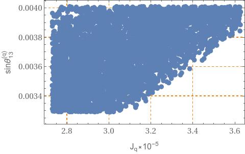
Figure 1: Correlation of the quark mixing parameter $\sin\theta^{(q)}_{13}$ with the Jarlskog invariant.

Finally, the LHC signature of the exotic $T$, $J_{1}$ and $J_{2}$ quarks in our model is defined by the fact that they will mainly decay into a top quark plus neutral scalar and can be pair produced at the LHC via Drell-Yan and gluon fusion processes mediated by charged gauge bosons and gluons, respectively. Consequently, we consider the observation of an excess of events in the multijet and multilepton final state as the smoking gun of our model at the LHC. A detailed study of the collider phenomenology of the model is beyond the scope of this paper and is left for future studies.

IV Meson oscillations

It is worth mentioning that the non universal $U(1)_{X}$ charge assignments for the left handed quark fields give rise to flavour changing neutral processes (FCNC) mediated by the $Z^{\prime}$ gauge boson. These FCNC interactions contribute to the $K^{0}-\bar{K}^{0}$, $B^{0}_{d}-\bar{B}^{0}_{d}$ and $B^{0}_{s}-\bar{B}^{0}_{s}$ mass differences. It is worth mentioning that the $D^{0}-\bar{D}^{0}$ meson oscillations are absent at tree level since the symmetries of our model constrain the up type quark mass matrix to be diagonal. In this section we discuss the implications of our model in the Flavour Changing Neutral Current (FCNC) interactions in the down type quark sector. The flavour violating $Z^{\prime}$ interactions in the down type quark sector produce meson oscillations. The $K^{0}-\bar{K}^{0}$, $B_{d}^{0}-\bar{B}_{d}^{0}$ and $B_{s}^{0}-\bar{B}_{s}^{0}$ meson mixings are described by the following effective Hamiltonians:

$$\mathcal{H}_{eff}^{\left(K^{0}-\bar{K}^{0}\right)}\mathcal{=}\frac{4\sqrt{2}G_{F}c_{W}^{4}m_{Z}^{2}}{\left(3-4s_{W}^{2}\right)m_{Z^{\prime}}^{2}}\left|\left(V_{DL}^{\ast}\right)_{32}\left(V_{DL}\right)_{31}\right|^{2}O^{\left(K^{0}-\bar{K}^{0}\right)},$$ (31)

$$\mathcal{H}_{eff}^{\left(B_{d}^{0}-\bar{B}_{d}^{0}\right)}\mathcal{=}\frac{4\sqrt{2}G_{F}c_{W}^{4}m_{Z}^{2}}{\left(3-4s_{W}^{2}\right)m_{Z^{\prime}}^{2}}\left|\left(V_{DL}^{\ast}\right)_{31}\left(V_{DL}\right)_{33}\right|^{2}O^{\left(B_{d}^{0}-\bar{B}_{d}^{0}\right)},$$ (32)

$$\mathcal{H}_{eff}^{\left(B_{s}^{0}-\bar{B}_{s}^{0}\right)}\mathcal{=}\frac{4\sqrt{2}G_{F}c_{W}^{4}m_{Z}^{2}}{\left(3-4s_{W}^{2}\right)m_{Z^{\prime}}^{2}}\left|\left(V_{DL}^{\ast}\right)_{32}\left(V_{DL}\right)_{33}\right|^{2}O^{\left(B_{s}^{0}-\bar{B}_{s}^{0}\right)}.$$ (33)

The $K^{0}-\bar{K}^{0}$, $B_{d}^{0}-\bar{B}_{d}^{0}$ and $B_{s}^{0}-\bar{B}_{s}^{0}$ meson mixings in our model is caused by the tree level $Z^{\prime}$ exchange, thus giving generating the following operators:

$$O^{\left(K^{0}-\bar{K}^{0}\right)} = \left(\overline{s}\gamma_{\mu}P_{L}d\right)\left(\overline{s}\gamma^{\mu}P_{L}d\right),\hskip 19.91684pt\hskip 19.91684ptO^{\left(B_{d}^{0}-\bar{B}_{d}^{0}\right)}=\left(\overline{d}\gamma_{\mu}P_{L}b\right)\left(\overline{d}\gamma^{\mu}P_{L}b\right),$$ (34)

$$O^{\left(B_{s}^{0}-\bar{B}_{s}^{0}\right)} = \left(\overline{s}\gamma_{\mu}P_{L}b\right)\left(\overline{s}\gamma^{\mu}P_{L}b\right).$$ (35)

Furthermore, the following relations have been taken into account:

$$\widetilde{M}_{f} = \left(M_{f}\right)_{diag}=V_{fL}^{\dagger}M_{f}V_{fR},\hskip 28.45274pt\hskip 28.45274ptf_{\left(L,R\right)}=V_{f\left(L,R\right)}\widetilde{f}_{\left(L,R\right)},$$

$$\overline{f}_{iL}\left(M_{f}\right)_{ij}f_{jR} = \overline{\widetilde{f}}_{kL}\left(V_{fL}^{\dagger}\right)_{ki}\left(M_{f}\right)_{ij}\left(V_{fR}\right)_{jl}\widetilde{f}_{lR}=\overline{\widetilde{f}}_{kL}\left(V_{fL}^{\dagger}M_{f}V_{fR}\right)_{kl}\widetilde{f}_{lR}=\overline{\widetilde{f}}_{kL}\left(\widetilde{M}_{f}\right)_{kl}\widetilde{f}_{lR}=m_{fk}\overline{\widetilde{f}}_{kL}\widetilde{f}_{kR},$$

$$k = 1,2,3\,.$$ (36)

Here, $\widetilde{f}_{k\left(L,R\right)}$ and $f_{k\left(L,R\right)}$ ($k=1,2,3$) are the SM fermionic fields in the mass and interaction bases, respectively.

It is worth mentioning as shown in detail in Appendix B, that our model has the alignment limit for the lightest $126$ GeV SM like Higgs boson given that the remaining scalars are much heavier than the electroweak symmetry breaking scale $246$ GeV. Furthermore, our model at low energies, below the scale the scale of breaking of the $SU(3)_{C}\times SU(3)_{L}\times U(1)_{X}$ gauge symmetry, corresponds to a multiscalar singlet extension of the SM. Thus, the light $126$ GeV Higgs boson will not induce tree-level FCNC. This phenomenologically dangerous effect can happen in the presence of at least two SM doublet scalars before the electroweak symmetry breaking. To avoid this trouble, one can resort to the Glashow-Weinberg-Paschos theorem [139, 140] stating that there will be no tree-level FCNC coming from the scalar sector, if all right-handed fermions of a given electric charge couple to only one of the doublets.

Besides that, the contributions to FCNC arising from the heavier scalars are strongly suppressed by their large mass scale and the very small mixings of the scalar singlets and the CP even neutral component of $\chi$ with the CP even electrically neutral component of $\eta$ (which is mostly composed of the $126$ GeV SM like Higgs boson). Because of this reason the FCNC interactions in our model mainly arise from the tree-level exchange of the $Z^{\prime}$ gauge boson. This situation is different than the one presented in 3-3-1 models with three scalar triplets like the ones considered in [69, 70, 71], where two of the three scalar triplets do acquire VEVs at the electroweak symmetry breaking scale thus implying that at low energies below the TeV scale, the theory corresponds to a 2HDM where tree-level neutral scalar contributions to FCNC do exist. This problem was elegantly solved in Refs. [69, 70, 71] by implementing the Froggatt-Nielsen mechanism in this version of the 3-3-1 model.

On the other hand, the $K-\bar{K}$, $B_{d}^{0}-\bar{B}_{d}^{0}$ and $B_{s}^{0}-\bar{B}_{s}^{0}$ mass splittings are given by:

$$\Delta m_{K}=\left(\Delta m_{K}\right)_{SM}+\Delta m_{K}^{\left(NP\right)},\hskip 28.45274pt\Delta m_{B_{d}}=\left(\Delta m_{B_{d}}\right)_{SM}+\Delta m_{B_{d}}^{\left(NP\right)},\hskip 28.45274pt\Delta m_{B_{s}}=\left(\Delta m_{B_{s}}\right)_{SM}+\Delta m_{B_{s}}^{\left(NP\right)},$$ (37)

where $\left(\Delta m_{K}\right)_{SM}$, $\left(\Delta m_{B_{d}}\right)_{SM}$ and $\left(\Delta m_{B_{s}}\right)_{SM}$ are the SM contributions, whereas $\Delta m_{K}^{\left(NP\right)}$ , $\Delta m_{B_{d}}^{\left(NP\right)}$ and $\left(\Delta m_{B_{s}}\right)_{SM}$ are new physics contributions.

In our model, the new physics contributions to the meson differences are given by:

$$\Delta m_{K}^{\left(NP\right)}=\frac{4\sqrt{2}G_{F}c_{W}^{4}m_{Z}^{2}}{\left(3-4s_{W}^{2}\right)m_{Z^{\prime}}^{2}}\left|\left(V_{DL}^{\ast}\right)_{32}\left(V_{DL}\right)_{31}\right|^{2}f_{K}^{2}B_{K}\eta_{K}m_{K},$$ (38)

$$\Delta m_{B_{d}}^{\left(NP\right)}=\frac{4\sqrt{2}G_{F}c_{W}^{4}m_{Z}^{2}}{\left(3-4s_{W}^{2}\right)m_{Z^{\prime}}^{2}}\left|\left(V_{DL}^{\ast}\right)_{31}\left(V_{DL}\right)_{33}\right|^{2}f_{B_{d}}^{2}B_{B_{d}}\eta_{B_{d}}m_{B_{d}},$$ (39)

$$\Delta m_{B_{s}}^{\left(NP\right)}=\frac{4\sqrt{2}G_{F}c_{W}^{4}m_{Z}^{2}}{\left(3-4s_{W}^{2}\right)m_{Z^{\prime}}^{2}}\left|\left(V_{DL}^{\ast}\right)_{32}\left(V_{DL}\right)_{33}\right|^{2}f_{B_{s}}^{2}B_{B_{s}}\eta_{B_{s}}m_{B_{s}}.$$ (40)

Using the following parameters [141, 142, 143, 144, 145, 146, 147]:

$$\Delta m_{K} = \left(3.484\pm 0.006\right)\times 10^{-12}MeV,\hskip 42.67912pt\left(\Delta m_{K}\right)_{SM}=3.483\times 10^{-12}MeV$$

$$f_{K} = 160MeV,\hskip 42.67912ptB_{K}=0.85,\hskip 42.67912pt\eta_{K}=0.57,\hskip 42.67912ptm_{K}=497.614MeV.$$

$$\left(\Delta m_{B_{d}}\right)_{\exp} = \left(3.337\pm 0.033\right)\times 10^{-10}MeV,\hskip 42.67912pt\left(\Delta m_{B_{d}}\right)_{SM}=3.582\times 10^{-10}MeV,$$

$$f_{B_{d}} = 188MeV,\hskip 42.67912ptB_{B_{d}}=1.26,\hskip 42.67912pt\eta_{B_{d}}=0.55,\hskip 42.67912ptm_{B_{d}}=5279.5MeV.$$

$$\left(\Delta m_{B_{s}}\right)_{\exp} = \left(104.19\pm 0.8\right)\times 10^{-10}MeV,\hskip 42.67912pt\left(\Delta m_{B_{s}}\right)_{SM}=121.103\times 10^{-10}MeV,$$

$$f_{B_{s}} = 225MeV,\hskip 42.67912ptB_{B_{s}}=1.26,\hskip 42.67912pt\eta_{B_{s}}=0.55,\hskip 42.67912ptm_{B_{s}}=5366.3MeV.$$

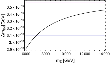
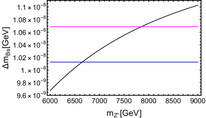
Figure 2: The $K^{0}-\bar{K}^{0}$, $B_{d}^{0}-\bar{B}_{d}^{0}$ and $B_{s}^{0}-\bar{B}_{s}^{0}$ mass splittings as as function of the $Z^{\prime}$ mass.

We plot in figure 2 the $K^{0}-\bar{K}^{0}$, $B_{d}^{0}-\bar{B}_{d}^{0}$ and $B_{s}^{0}-\bar{B}_{s}^{0}$ mass splittings as as function of the $Z^{\prime}$ mass. As seen from figure 2, the $K^{0}-\bar{K}^{0}$, $B_{d}^{0}-\bar{B}_{d}^{0}$ and $B_{s}^{0}-\bar{B}_{s}^{0}$ oscillations caused by the flavor changing neutral interactions reach values close to their experimental upper limits and the constraints arising from these meson oscillations set the $Z^{\prime}$ mass in the range $7$ TeV$\lesssim m_{Z^{\prime}}\lesssim 8$ TeV.

V Lepton masses and mixings

From the charged lepton Yukawa terms, we find the charged lepton mass matrix in the form:

$$M_{l} = \left(\begin{array}[]{ccc}a_{1}\lambda^{9}+b_{1}\lambda^{9}\left(\cos(\alpha)-e^{-i\psi}\sin(\alpha)\right)&b_{2}\lambda^{5}\left(\cos(\alpha)+e^{i\psi}\sin(\alpha)\right)&a_{3}\lambda^{3}+b_{3}\lambda^{3}\left(\cos(\alpha)-e^{-i\psi}\sin(\alpha)\right)\\ a_{1}\lambda^{9}+b_{1}\lambda^{9}\omega^{2}\left(\cos(\alpha)-e^{-i\psi}\omega^{2}\sin(\alpha)\right)&b_{2}\lambda^{5}\omega\left(\cos(\alpha)+e^{i\psi}\omega\sin(\alpha)\right)&a_{3}\lambda^{3}+b_{3}\lambda^{3}\omega^{2}\left(\cos(\alpha)-e^{-i\psi}\omega^{2}\sin(\alpha)\right)\\ a_{1}\lambda^{9}+b_{1}\lambda^{9}\omega\left(\cos(\alpha)-e^{-i\psi}\omega\sin(\alpha)\right)&b_{2}\lambda^{9}\omega^{2}\left(\cos(\alpha)+e^{i\psi}\omega^{2}\sin(\alpha)\right)&a_{3}\lambda^{3}+b_{3}\lambda^{3}\omega\left(\cos(\alpha)-e^{-i\psi}\omega\sin(\alpha)\right)\\ \end{array}\right)$$

$$\times\frac{v_{\eta}}{\sqrt{2}},$$

where $a_{1}$, $a_{3}$, $b_{i}$ ($i=1,2,3$) are $\mathcal{O}(1)$ parameters constructed of the parameters $y^{(L)}_{i},z^{(L)}$. Note that the charged lepton masses are linked to the scale of the electroweak symmetry breaking through their power dependence on the Wolfenstein parameter $\lambda$, with $\mathcal{O}(1)$ coefficients. Furthermore, from the lepton Yukawa terms given in Eq. (18) it follows that our model does not feature flavor changing leptonic neutral Higgs decays at tree level.

For the neutrino sector we find from Eq. (18) the neutrino mass term:

$$-2\mathcal{L}_{mass}^{(\nu)}=\left(\begin{array}[]{ccc}\overline{\nu_{L}^{\ C}}&\overline{\nu_{R}}&\overline{N_{R}}\end{array}\right)M_{\nu}\left(\begin{array}[]{c}\nu_{L}\\ \nu_{R}^{\ C}\\ N_{R}^{\ C}\end{array}\right)+H.c,$$ (46)

where $\nu_{iR}\equiv((\nu^{c})_{L})^{C}$ corresponds to the third components of the lepton triplet introduced in Eq. (4). The $A_{4}$ family symmetry of the model constrains the neutrino mass matrix to be of the form:

$$M_{\nu}=\left(\begin{array}[]{ccc}0_{3\times 3}&M_{1}&M_{2}\\ M_{1}^{T}&0_{3\times 3}&M_{3}\\ M_{2}^{T}&M_{3}^{T}&0_{3\times 3}\end{array}\right)$$ (47)

with

$$M_{1} = \frac{v_{\eta}v_{\chi}v_{\zeta}}{2\sqrt{2}\Lambda^{2}}\left(\frac{v_{\sigma}}{\Lambda}\right)^{11}\left(\begin{array}[]{ccc}0&\omega^{2}&0\\ -\omega^{2}&0&1\\ 0&-1&0\end{array}\right),\hskip 28.45274pt\hskip 28.45274ptM_{2}=y_{1\eta}^{(L)}\frac{v_{\eta}v_{\xi}}{\sqrt{6}\Lambda}\left(\frac{v_{\sigma}}{\Lambda}\right)\left(\begin{array}[]{ccc}0&(1+x)\omega^{2}&(1-x)\omega\\ (1-x)\omega^{2}&0&1+x\\ (1+x)\omega&1-x&0\end{array}\right),$$ (54)

$$M_{3} = y_{\chi}^{(L)}\frac{v_{\chi}}{\sqrt{2}}\left(\frac{v_{\sigma}}{\Lambda}\right)\left(\begin{array}[]{ccc}1&0&0\\ 0&\omega&0\\ 0&0&\omega^{2}\end{array}\right),\hskip 28.45274pt\hskip 28.45274ptx=\frac{y_{2\eta}^{(L)}}{y_{1\eta}^{(L)}},\hskip 28.45274pt\hskip 28.45274pt\omega=e^{\frac{2\pi i}{3}}.$$ (58)

The light active masses arise from linear seesaw mechanism and the physical neutrino mass matrices are:

$$M_{\nu}^{(1)} = -\left[M_{2}M_{3}^{-1}M_{1}^{T}+M_{1}\left(M_{3}^{T}\right)^{-1}M_{2}^{T}\right]\,,$$ (59)

$$M_{\nu}^{(2)} = -\frac{1}{2}\left(M_{3}+M_{3}^{T}\right)+\frac{1}{4}\left[M_{1}^{T}(M_{3}^{\ast})^{-1}M_{2}^{\ast}+M_{2}^{\dagger}(M_{3}^{\dagger})^{-1}M_{1}\right]\,,$$ (60)

$$M_{\nu}^{(3)} = \frac{1}{2}\left(M_{3}+M_{3}^{T}\right)+\frac{1}{4}\left[M_{1}^{T}(M_{3}^{\ast})^{-1}M_{2}^{\ast}+M_{2}^{\dagger}(M_{3}^{\dagger})^{-1}M_{1}\right]\,\,,$$ (61)

where $M_{\nu}^{(1)}$ is the active neutrino mass matrix whereas $M_{\nu}^{(2)}$ and $M_{\nu}^{(3)}$ are the sterile neutrino mass matrices. Explicitly we have

$$M_{\nu}^{(1)} = \frac{y_{1\eta}^{(L)}}{\sqrt{2}y_{\chi}^{(L)}}\left(\frac{v_{\sigma}}{\Lambda}\right)^{11}\frac{v_{\eta}v_{\zeta}v_{\xi}}{\Lambda^{3}}\left(\begin{array}[]{ccc}-2(x+1)&\omega^{2}(x-1)&2\omega x\\ \omega^{2}(x-1)&-4\omega x&x+1\\ 2\omega x&x+1&-2\omega^{2}(x-1)\end{array}\right)\frac{v_{\eta}}{\sqrt{2}}$$ (65)

$$= \left(\begin{array}[]{ccc}-2(x+1)&\omega^{2}(x-1)&2\omega x\\ \omega^{2}(x-1)&-4\omega x&x+1\\ 2\omega x&x+1&-2\omega^{2}(x-1)\end{array}\right)m_{\nu},\hskip 28.45274ptm_{\nu}=\frac{a_{\nu}\lambda^{19}v}{\sqrt{2}}\,.$$ (69)

The experimental values of charged lepton masses, the neutrino mass squared splittings, the leptonic mixing parameters and Dirac CP violating phase can be reproduced for the normal ordering (NO) of the neutrino mass spectrum with the following values of the model effective parameters:

$$\begin{array}[]{c}a_{1}\simeq 0.983,\hskip 28.45274pta_{3}\simeq-0.483,\hskip 28.45274ptb_{1}\simeq-0.755,\hskip 28.45274ptb_{2}\simeq-0.597,\hskip 28.45274ptb_{3}\simeq-0.199,\hskip 28.45274ptx\simeq 0.431,\\ m_{\nu}\simeq 16.34\ \mbox{meV},\hskip 28.45274pt\alpha\simeq 122.25^{\circ}\,,\hskip 28.45274pt\beta\simeq-42.82^{\circ}\,,\hskip 28.45274pt\gamma\simeq-59.36^{\circ}\,,\hskip 28.45274pt\psi\simeq 98.44^{\circ}\,.\end{array}$$ (70)

Using the values of the lepton model effective parameters of Eq. (70), the PMNS leptonic mixing matrix takes the form:

$$U_{PMNS}=U^{\dagger}_{l}U_{\nu}=\left(\begin{array}[]{ccc}-0.818231-0.0686404i&-0.318382+0.449127i&0.148954\,+0.0227392i\\ 0.0515003\,+0.373766i&-0.379958-0.371145i&0.731222\,+0.202101i\\ -0.180118-0.388575i&0.634519\,-0.110392i&0.564605\,-0.288074i\\ \end{array}\right)$$ (71)

where:

$$U_{l} = \left(\begin{array}[]{ccc}-0.625827&-0.614417&-0.48045\\ -0.406057-0.298325i&0.726662\,+0.202306i&-0.400359+0.129878i\\ 0.569876\,-0.172341i&-0.112245-0.202306i&-0.59877+0.483205i\\ \end{array}\right),$$ (75)

$$U_{\nu} = \left(\begin{array}[]{ccc}0.566967&0.12785&-0.813759\\ 0.396158\,+0.686167i&-0.177447-0.307348i&0.248135\,+0.429782i\\ -0.112675+0.195159i&-0.463062+0.802046i&-0.151256+0.261983i\\ \end{array}\right).$$ (79)

As seen from Table 4, the model values are consistent with the experimental ones. Again, akin to the quark sector, the absolute value of the effective dimensionless parameters $a^{(l)},x$ are of the order of unity. We interpret this fact in a way that the lepton mass hierarchy is explained on account of the model structure, symmetries and field content, without unnatural tuning these effective parameters.

Observable	Model	bpf $\pm 1\sigma$ [148]	bpf $\pm 1\sigma$ [149]	$2\sigma$ range [148]	$3\sigma$ range [148]	$3\sigma$ range [149]
$\Delta m_{21}^{2}$ [$10^{-5}$eV2]	$7.59$	$7.55_{-0.16}^{+0.20}$	$7.40_{-0.20}^{+0.21}$	$7.20-7.94$	$7.05-8.14$	$6.80-8.02$
$\Delta m_{31}^{2}$ [$10^{-3}$eV2]	$2.53$	$2.50\pm 0.03$	$2.494_{-0.031}^{+0.033}$	$2.44-2.57$	$2.41-2.60$	$2.399-2.593$
$\theta^{(l)}_{12}(^{\circ})$	$33.84$	$34.5_{-1.0}^{+1.2}$	$36.62_{-0.76}^{+0.78}$	$32.5-36.8$	$31.5-38.0$	$31.42-36.05$
$\theta^{(l)}_{13}(^{\circ})$	$8.67$	$8.45_{-0.14}^{+0.16}$	$8.54\pm 0.15$	$8.2-8.8$	$8.0-8.9$	$8.09-8.98$
$\theta^{(l)}_{23}(^{\circ})$	$50.12$	$47.9_{-1.7}^{+1.0}$	$47.2_{-3.9}^{+1.9}$	$43.1-49.8$	$41.8-50.7$	$40.3-51.5$
$\delta^{(l)}_{CP}(^{\circ})$	$-85.29$	$-142_{-27}^{+38}$	$-108_{-31}^{+43}$	$182-315$	$157-349$	$144-374$

Table 4: Model and experimental values of the light active neutrino masses, leptonic mixing angles and CP violating phase for the scenario of normal (NH) neutrino mass hierarchy. The experimental values are taken from Refs. [148, 149]

Figure 3 shows the correlations of the leptonic mixing angles with the leptonic Dirac CP-violating phase as well as the correlations between the leptonic mixing parameters. To obtain these Figures, the lepton sector parameters were randomly generated in a range of values where the neutrino mass squared splittings, leptonic mixing parameters and leptonic Dirac CP violating phase are consistent with the experimental data. These lepton sector observables are inside the $1\sigma$ experimentally allowed range, excepting $\theta^{(l)}_{23}$ which is inside the $3\sigma$ range. We found the leptonic Dirac CP violating phase in the range $-90^{\circ}\lesssim\delta^{(l)}_{CP}\lesssim-25^{\circ}$, whereas the leptonic mixing angles are obtained to be in the ranges $31.5^{\circ}\lesssim\theta^{(l)}_{12}\lesssim 37.5^{\circ}$, $48.0^{\circ}\lesssim\theta^{(l)}_{23}\lesssim 51.5^{\circ}$ and $8.15^{\circ}\lesssim\theta^{(l)}_{12}\lesssim 8.9^{\circ}$.

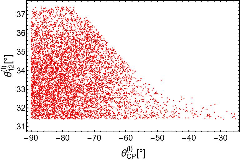
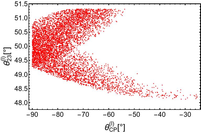
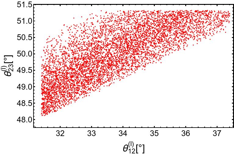
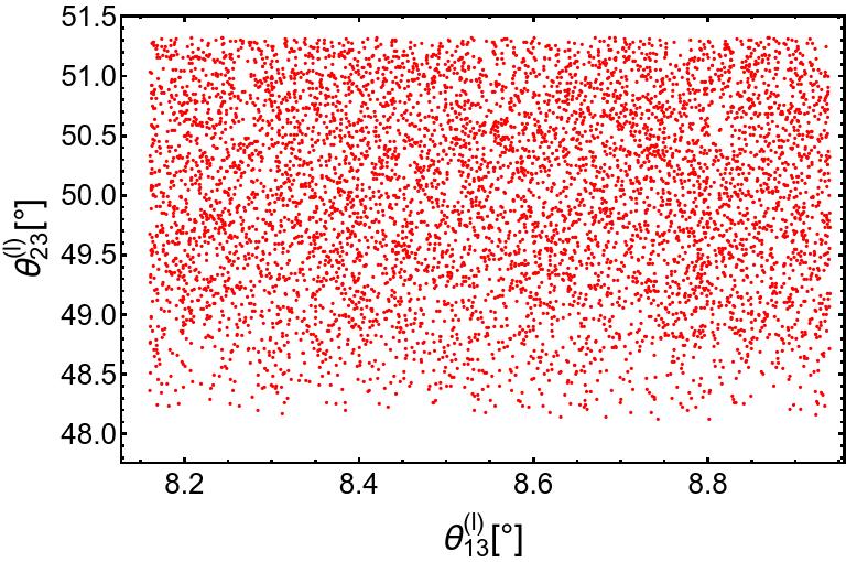
Figure 3: Correlations between the different lepton sector observables.

Let us consider the effective Majorana neutrino mass parameter

$$m_{\beta\beta}=\left|\sum_{j}U_{ek}^{2}m_{\nu_{k}}\right|,$$ (80)

where $U_{ej}$ and $m_{\nu_{k}}$ are the the PMNS leptonic mixing matrix elements and the neutrino Majorana masses, respectively. The neutrinoless double beta ($0\nu\beta\beta$) decay amplitude is proportional to $m_{\beta\beta}$.

Fig. 4 shows the correlation of the effective Majorana neutrino mass parameter $m_{ee}$ vs the lightest neutrino mass $m_{1}$.

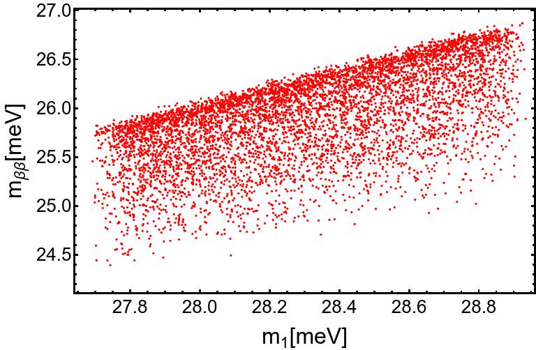
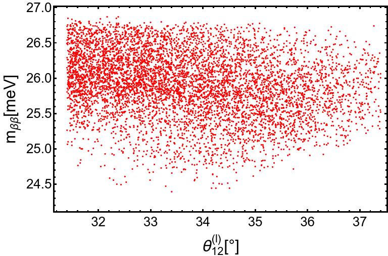
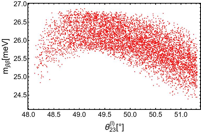
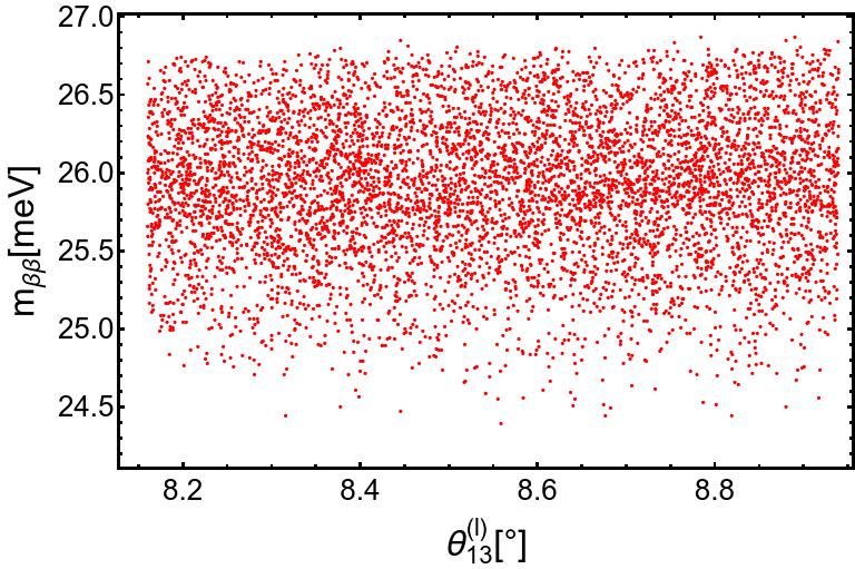
Figure 4: Correlations of the effective Majorana neutrino mass parameter $m_{\beta\beta}$ with the lightest neutrino mass $m_{1}$ and with the leptonic mixing parameters.

As can be seen from Fig. 4, our model predicts the values of the effective Majorana neutrino mass parameter in the range $24.5$ meV$\lesssim m_{\beta\beta}\lesssim$ $27$ meV, which is within the declared reach of the next-generation bolometric CUORE experiment [150] or, more realistically, of the next-to-next-generation ton-scale $0\nu\beta\beta$-decay experiments. The current most stringent experimental upper limit $m_{\beta\beta}\leq 160$ meV is set by $T_{1/2}^{0\nu\beta\beta}(^{136}\mathrm{Xe})\geq 1.1\times 10^{26}$ yr at 90% C.L. from the KamLAND-Zen experiment [151].

VI $Z^{\prime}$ gauge boson production at the LHC

Here we compute the total cross section for the production of the heavy $Z^{\prime}$ gauge boson, defined in Eq (10), at the LHC via Drell-Yan mechanism. We consider the dominant contribution due to the parton distribution functions of the light up, down and strange quarks, so that the total cross section for the production of a $Z^{\prime}$ via quark antiquark annihilation in proton-proton collisions with center of mass energy $\sqrt{S}$ takes the form:

$$\sigma_{pp\rightarrow Z^{\prime}}^{\left(DrellYan\right)}(S) = \frac{g^{2}\pi}{6c_{W}^{2}S}\left\{\left[\left(g_{uL}^{\prime}\right)^{2}+\left(g_{uR}^{\prime}\right)^{2}\right]\int_{\ln\sqrt{\frac{m_{Z^{\prime}}^{2}}{S}}}^{-\ln\sqrt{\frac{m_{Z^{\prime}}^{2}}{S}}}f_{p/u}\left(\sqrt{\frac{m_{Z^{\prime}}^{2}}{S}}e^{y},\mu^{2}\right)f_{p/\overline{u}}\left(\sqrt{\frac{m_{Z^{\prime}}^{2}}{S}}e^{-y},\mu^{2}\right)dy\right.$$ (81)

$$+\left.\left[\left(g_{dL}^{\prime}\right)^{2}+\left(g_{dR}^{\prime}\right)^{2}\right]\int_{\ln\sqrt{\frac{m_{Z^{\prime}}^{2}}{S}}}^{-\ln\sqrt{\frac{m_{Z^{\prime}}^{2}}{S}}}f_{p/d}\left(\sqrt{\frac{m_{Z^{\prime}}^{2}}{S}}e^{y},\mu^{2}\right)f_{p/\overline{d}}\left(\sqrt{\frac{m_{Z^{\prime}}^{2}}{S}}e^{-y},\mu^{2}\right)dy\right.$$

$$+\left.\left[\left(g_{dL}^{\prime}\right)^{2}+\left(g_{dR}^{\prime}\right)^{2}\right]\int_{\ln\sqrt{\frac{m_{Z^{\prime}}^{2}}{S}}}^{-\ln\sqrt{\frac{m_{Z^{\prime}}^{2}}{S}}}f_{p/s}\left(\sqrt{\frac{m_{Z^{\prime}}^{2}}{S}}e^{y},\mu^{2}\right)f_{p/\overline{s}}\left(\sqrt{\frac{m_{Z^{\prime}}^{2}}{S}}e^{-y},\mu^{2}\right)dy\right\}\,,$$

where $g_{uL(R)}^{\prime}$, $g_{dL(R)}^{\prime}$ are the $Z^{\prime}$ couplings to left (right) handed up and down type quarks, respectively. These couplings are given in Appendix D. The functions $f_{p/u}\left(x_{1},\mu^{2}\right)$ ($f_{p/\overline{u}}\left(x_{2},\mu^{2}\right)$), $f_{p/d}\left(x_{1},\mu^{2}\right)$ ($f_{p/\overline{d}}\left(x_{2},\mu^{2}\right)$) and $f_{p/s}\left(x_{1},\mu^{2}\right)$ ($f_{p/\overline{s}}\left(x_{2},\mu^{2}\right)$) are the distributions of the light up, down and strange quarks (antiquarks), respectively, in the proton which carry momentum fractions $x_{1}$ ($x_{2}$) of the proton.

The factorization scale is taken to be $\mu=m_{Z^{\prime}}$.

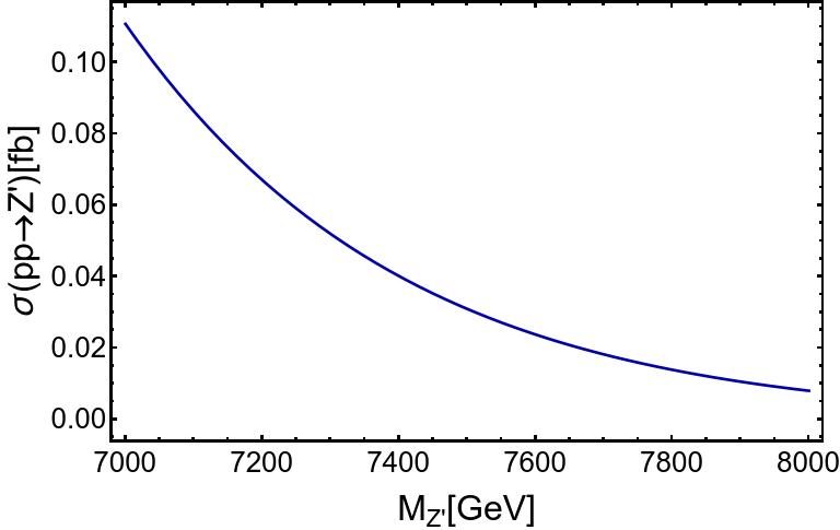
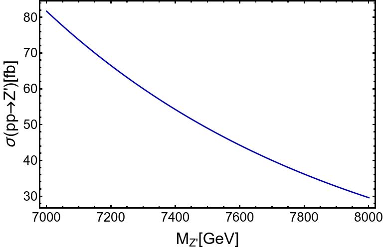
Figure 5: Total cross section for the $Z^{\prime}$ production via Drell-Yan mechanism at the LHC for $\sqrt{S}=13$ TeV (left plot) and $\sqrt{S}=28$ TeV (right plot) and as a function of the $Z^{\prime}$ mass.

Fig. 5 (left panel) displays the $Z^{\prime}$ total production cross section at the LHC via the Drell-Yan mechanism for $\sqrt{S}=13$ TeV as a function of the $Z^{\prime}$ mass $M_{Z^{\prime}}$ in the range from $7$ TeV up to $8$ TeV. We consider $M_{Z^{\prime}}\geq 7$ TeV in order to fulfill the bound arising from the experimental data on $K$, $B_{d}$ and $B_{s}$ meson mixings obtained in section IVFor this region of $Z^{\prime}$ masses we find that the total production cross section ranges from $0.11$ fb up to $0.01$ fb. The heavy neutral $Z^{\prime}$ gauge boson, after being produced, will subsequently decay into the pair of the SM particles, with the dominant decay mode into quark-antiquark pairs as shown in Refs. [152, 9]. The two body decays of the $Z^{\prime}$ gauge boson in 3-3-1 models have been studied in details in Ref. [152]. In particular, in Ref. [152] it has been shown that in 3-3-1 models the $Z^{\prime}$ decays into a lepton pair have branching ratios of the order of $10^{-2}$, which implies that the total LHC cross section for the $pp\to Z^{\prime}\to l^{+}l^{-}$ resonant production at $\sqrt{S}=13$ TeV will be of the order of $10^{-3}$ fb for a $7$ TeV $Z^{\prime}$ gauge boson, which is below its corresponding lower experimental limit from the LHC searches [153]. On the other hand, at the proposed energy upgrade of the LHC up to 28 TeV center of mass energy, the total cross section for the Drell-Yan production of a heavy $Z^{\prime}$ neutral gauge boson gets significantly enhanced reaching values ranging from $82$ fb up to $30$ fb, as indicated in the right panel of Fig. 5. Consequently, the LHC cross section for the $pp\to Z^{\prime}\to l^{+}l^{-}$ resonant production at $\sqrt{S}=28$ TeV will be of the order of $1$ fb for a $7$ TeV $Z^{\prime}$ gauge boson, which is consisteny with its corresponding lower experimental limit arising from the LHC searches [153].

VII Lepton flavour violating decays

Let us analyze the implications of our model for the LFV decays of the SM charged leptons and Higgs boson.

Given that the SM charged lepton mass matrix (94) cannot be diagonalized analytically in the practically useful form, in this section, for the sake of simplicity, we restrict ourselves to a simplified benchmark scenario characterized by the relations:

$$z_{1}^{(L)}=y_{1}^{(L)},\ \ v_{\phi}=e^{i\gamma}\sin\beta v_{\varphi},\ \ v_{\rho}=v_{\varphi}\cos\beta,\ \ y_{3}^{(L)}=-e^{-i\gamma}y_{4}^{(L)}\tan\beta,\hskip 28.45274ptz_{3}^{(L)}=e^{-i\gamma}y_{4}^{(L)}\cot\beta.$$ (82)

Then, the charged lepton mass matrix takes the form:

$$M_{l} = R_{lL}diag\left(m_{e},m_{\mu},m_{\tau}\right),\hskip 28.45274ptR_{lL}=\frac{1}{\sqrt{3}}\left(\begin{array}[]{ccc}1&1&1\\ 1&\omega&\omega^{2}\\ 1&\omega^{2}&\omega\end{array}\right)\left(\begin{array}[]{ccc}1&0&0\\ 0&\cos\alpha&-\sin\alpha e^{-i\psi}\\ 0&\sin\alpha e^{i\psi}&\cos\alpha\end{array}\right)\left(\begin{array}[]{ccc}\cos\beta&0&-\sin\beta e^{-i\gamma}\\ 0&1&0\\ \sin\beta e^{i\gamma}&0&\cos\beta\end{array}\right),$$ (92)

$$\omega = e^{\frac{2\pi i}{3}},$$ (93)

where the charged lepton masses are:

$$m_{e}=a_{1}^{(l)}\lambda^{9}\frac{v}{\sqrt{2}},\hskip 28.45274ptm_{\mu}=a_{2}^{(l)}\lambda^{5}\frac{v}{\sqrt{2}},\hskip 28.45274ptm_{\tau}=a_{3}^{(l)}\lambda^{3}\frac{v}{\sqrt{2}}.$$ (94)

In Appendix B we derived an expression (B) for the SM Higgs boson, $h^{0}_{1}$, as a linear combination of the scalars present in our model. We combine such relations with the definitions of the charged lepton mass eigenstates and masses:

$$\widetilde{M}_{f} = \left(M_{f}\right)_{diag}=V_{fL}^{\dagger}M_{f}V_{fR},\hskip 28.45274pt\hskip 28.45274ptf_{\left(L,R\right)}=V_{f\left(L,R\right)}\widetilde{f}_{\left(L,R\right)},$$

$$\overline{f}_{iL}\left(M_{f}\right)_{ij}f_{jR} = \overline{\widetilde{f}}_{kL}\left(V_{fL}^{\dagger}\right)_{ki}\left(M_{f}\right)_{ij}\left(V_{fR}\right)_{jl}\widetilde{f}_{lR}=\overline{\widetilde{f}}_{kL}\left(V_{fL}^{\dagger}M_{f}V_{fR}\right)_{kl}\widetilde{f}_{lR}=\overline{\widetilde{f}}_{kL}\left(\widetilde{M}_{f}\right)_{kl}\widetilde{f}_{lR}=m_{fk}\overline{\widetilde{f}}_{kL}\widetilde{f}_{kR},$$

$$k = 1,2,3\,.$$ (95)

where $\widetilde{f}_{k\left(L,R\right)}$ and $f_{k\left(L,R\right)}$ ($k=1,2,3$) are the SM fermion mass and interaction eigenstates, respectively.

Then, considering the first three terms in Eq.  (18) we find the $h^{0}_{1}ee$ couplings

$$-\mathcal{L}_{h^{0}_{1}ee} \subset\left(1+\frac{\xi_{\eta}}{v_{\eta}}+\frac{\xi_{\chi}}{v_{\chi}}\right)\left(m_{e_{i}}\overline{e_{iL}}e_{iR}+\mathrm{H.c.}\right)\rightarrow\frac{g}{2m_{W}}\left(c_{\alpha}+s_{\alpha}t_{\theta}\right)h^{0}_{1}\left(m_{e_{i}}\overline{e_{iL}}e_{iR}+\mathrm{H.c.}\right),$$ (96)

coinciding in the limit $s_{\alpha}\to 0$ with the SM ones. As seen from the above formula, there are no lepton flavor violating decays of the SM-like Higgs bosons (LFVHD) $h^{0}_{1}\rightarrow e_{i}^{\pm}e_{j}^{\mp}$ with $i\neq j$ at tree level. This is consistent with the latest experimental result, where no signals were found setting the upper bound Br$(h^{0}_{1}\rightarrow\tau^{\mp}\mu^{\pm},\tau^{\mp}e^{\pm})<\mathrm{O}(10^{-3})$ at 95 % confidence level [154, 155]. This feature distinguishes our model from some previous models with discrete symmetry that predicted tree-level LFVHD [156]. However, the SM-like Higgs bosons in our model still couple with the heavy neutrinos through the four last Yukawa terms in Eq. (18). Hence, the LFVHD may arise at one-loop level, as in the models of the standard seesaw, inverse seesaw, and 3-3-1 model with massive neutrinos and inverse seesaw mechanism [157, 158, 159, 160, 161, 162]. While the standard seesaw model predicts suppressed branching ratios for LFVHD, these branchings can reach interesting values of the order of $10^{-5}$ in the models with inverse seesaw mechanisms. Recent studies predict that the experimental sensitivities for LFVHD can reach values of the order of $10^{-5}$ in the near future [163, 164].

The one-loop diagrams contributing to the LFV decays of $e_{i}\rightarrow e_{j}\gamma$ and the SM-like Higgs boson decay $h^{0}_{1}\rightarrow e_{i}e_{j}$ with $i\neq j$ are exactly the same as those that appear in the seesaw and inverse seesaw versions of the SM. The difference is the neutrino mixing matrix, arising from the linear seesaw mechanism. Hence, it will be interesting to estimate how large the Br$(h^{0}_{1}\rightarrow e_{i}e_{j})$ can become under the current bounds of Br$(\mu\rightarrow e\gamma)<4.2\times 10^{-13}$ [165]. It is expected that the future experimental sensitivities to the LFV decays will be improved, namely $6\times 10^{-14}$ for Br$(\mu\rightarrow\,e\gamma)$ [166, 167], and about $\mathcal{O}(10^{-9})$ for the two decays Br$(\tau\rightarrow\,e\gamma)$ and Br$(\tau\rightarrow\,\mu\gamma)$ [168] (for a recent review see, for instance, Ref. [169]).

We will use the approximate formulas for the Br$(e_{i}\rightarrow e_{j}\gamma)$ in 3-3-1 models given in Ref. [170], which were checked to be well-consistent with the results obtained from the exact numerical computation. Other approaches used for discussions of LFV decays of charged leptons in 3-3-1 models were also given previously in the literature [28, 171, 172]. Analytic formulas for calculating the one-loop contributions to LFVHD in the unitary gauge are given in Ref. [161, 162, 32], and were shown to be consistent with previous works [160]. Using these formulas, we only determine couplings between physical states and ignore all Goldstone bosons.

From the definition of the $SU(3)_{L}\times U(1)_{X}$ covariant derivative (7) we find its part related with the charged gauge bosons in our model

$$\Pi^{CC}_{\mu}\equiv\frac{1}{\sqrt{2}}\begin{pmatrix}0&W^{+}_{\mu}&0\\ W^{-}_{\mu}&0&Y^{-}_{\mu}\\ 0&Y^{+}_{\mu}&0\end{pmatrix}.$$ (97)

Hence the couplings of the SM-like Higgs with the charged gauge bosons are given by:

$$\mathcal{L}_{h^{0}_{1}VV} \subset\left(D_{\mu}\eta\right)^{\dagger}\left(D^{\mu}\eta\right)+\left(D_{\mu}\chi\right)^{\dagger}\left(D^{\mu}\chi\right),$$

$$\mathcal{L}_{h^{0}_{1}VV} =g\,m_{W}c_{\alpha}h^{0}_{1}W^{+\mu}W^{-}_{\mu}+g\,m_{Y}h^{0}_{1}s_{\alpha}Y^{+\mu}Y^{-}_{\mu}.$$ (98)

The matrix $U_{lL}$ in Eq. (93) will be used to change the basis of the left-handed charged leptons from the flavor basis to the physical one. Specifically, the correspondence between the original basis of the left-handed leptons and the physical one is $\overline{e_{L}}R_{lL}\leftrightarrow\overline{e_{L}}$, or $e_{L}\leftrightarrow R_{lL}e_{L}$, while the right handed ones are unchanged. This means that $e_{iL}\to U_{lL,ij}e_{jL}$ and $\overline{e_{iL}}\to\overline{e_{jL}}U^{\dagger}_{lL,ji}$ with $i,j=1,2,3$.

From Eqs. (96) and (VII), we note that the couplings SM-like Higgs boson with normal charged leptons and gauge boson $W^{\pm}$ in the model under consideration ans the SM are $(c_{\alpha}+s_{\alpha}t_{\theta})$ and $c_{\alpha}$, respectively. The lower bound $m_{Z^{\prime}}\geq 4$ TeV gives $v_{\chi}\geq 10$ TeV, which results in small $s_{\alpha}\simeq t_{2\alpha}/2\sim t_{\theta}\sim v/v_{\chi}\sim\mathcal{O}(10^{-2})$, therefore $c_{\alpha}=1+\mathcal{O}(10^{-4})$. Similarly for the couplings of SM-like Higgs bosons with the SM quarks and the neutral gauge boson $Z$, where $\xi_{\eta}$ plays role of the SM Higgs boson after the first breaking step. After the second one, the physical state of the SM-like Higgs boson is $h^{0}_{1}\simeq c_{\alpha}\xi_{\eta}$ and the relative difference the Z boson with other particle is $c_{\phi}$ with $s_{\phi}\sim v^{2}/v^{2}_{\chi}$ given in Eq. (133). Hence, the largest relative differences between the couplings of the $h^{0}_{1}$ predicted by our model and the SM are $c_{\alpha}$ and $c_{\alpha}c_{\phi}$. As a consequence, these couplings of the SM-like Higgs bosons are still in the allowed regions constrained from experiments.

The neutrino mass matrix $M_{\nu}$ in Eq. (47) is diagonalized via an unitary $9\times 9$ matrix $U_{\nu}$, namely

$$U_{\nu}^{T}M_{\nu}U_{\nu} =\hat{M}_{\nu}=\mathrm{diag}(m_{n_{1}},m_{n_{2}},...,\hat{m}_{n_{9}})=\mathrm{diag}(\hat{m}_{\nu},\;\hat{m}_{N}),$$ (99)

where $\hat{m}_{\nu}=\mathrm{diag}(m_{n_{1}},\;m_{n_{2}},\;m_{n_{3}})$ and $\hat{m}_{N}=\mathrm{diag}(m_{n_{4}},\;m_{n_{5}},...,\;m_{n_{9}})$ are the masses of active and exotic neutrinos $n_{L}=(n_{1L},n_{2L},...,n_{9L})$. They are Majorana fermions that satisfy $n_{kR}=n^{c}_{kL}$ with $k=1,2,...,9$. Relations between the interaction and physical basis for the neutrino fields are: $(\overline{\nu^{C}_{L}}\quad\overline{\nu_{R}}\quad\overline{N_{R}})=\overline{n_{R}}U^{T}_{\nu}$ and $(\nu_{L}\quad\nu^{C}_{R}\quad N^{C}_{R})^{T}=U_{\nu}n_{L}$.

The couplings of charged gauge bosons with leptons are given by

$$\mathcal{L}_{V^{\pm}\ell\ell} =i(\overline{L_{L}}\gamma^{\mu}P^{CC}_{\mu}L_{L})_{1}=\frac{g}{\sqrt{2}}\left(\overline{e_{iL}}\gamma^{\mu}\nu_{iL}W^{-}_{\mu}+\overline{e_{iL}}\gamma^{\mu}(\nu^{c}_{i})_{L}Y^{-}_{\mu}+\mathrm{H.c.}\right).$$

$$\rightarrow\mathcal{L}_{V^{\pm}\ell\ell} =\frac{g}{\sqrt{2}}\left[(U_{lL})_{ji}(U_{\nu})_{ik}\overline{e_{jL}}\gamma^{\mu}n_{kL}W^{-}_{\mu}+(U_{lL})_{ji}(U_{\nu})_{(i+3)k}\overline{e_{jL}}\gamma^{\mu}n_{kL}Y^{-}_{\mu}+\mathrm{H.c.}\right],$$ (100)

where the sums are taken for $i,j=1,2,3$ and $k=1,2,..,9$, and we have used $(\nu^{c}_{i})_{L}=\nu^{C}_{iR}$.

Based on Eq. (18), couplings of SM-like Higgs boson with neutrinos are included in the following interactions:

$$-\mathcal{L}_{h^{0}_{1}nn} \subset\left(1+\frac{\xi_{\eta}}{v_{\eta}}+\frac{\xi_{\chi}}{v_{\chi}}\right)\left[\overline{\nu^{C}_{L}}M_{1}\nu^{C}_{R}+\mathrm{H.c.}\right]+\left(1+\frac{\xi_{\eta}}{v_{\eta}}\right)\left[\overline{\nu^{C}_{L}}M_{2}N^{C}_{R}+\mathrm{H.c.}\right]+\left(1+\frac{\xi_{\chi}}{v_{\chi}}\right)\left[\overline{\nu_{R}}M_{3}N^{C}_{R}+\mathrm{H.c.}\right],$$

$$-\mathcal{L}_{h^{0}_{1}nn} =\frac{g}{2m_{W}}h^{0}_{1}\left[\left(c_{\alpha}+s_{\alpha}t_{\theta}\right)\left(\overline{\nu^{C}_{L}}M_{1}\nu^{C}_{R}+\mathrm{H.c.}\right)+c_{\alpha}\left(\overline{\nu^{C}_{L}}M_{2}N^{C}_{R}+\mathrm{H.c.}\right)+s_{\alpha}t_{\theta}\left(\overline{\nu^{C}_{L}}M_{3}N^{C}_{R}+\mathrm{H.c.}\right)\right]$$

$$=\frac{gc_{\alpha}}{2m_{W}}h^{0}_{1}\left[\left(1+t_{\alpha}t_{\theta}\right)(U_{\nu})_{ik}(M_{1})_{ij}(U_{\nu})_{(j+3)p}+(U_{\nu})_{ik}(M_{2})_{ij}(U_{\nu})_{(j+6)p}\right.$$

$$+\left.t_{\alpha}t_{\theta}(U_{\nu})_{(i+3)k}(M_{3})_{ij}(U_{\nu})_{(j+6)p}\right]\overline{n_{kR}}n_{pL}+\mathrm{H.c}.,$$ (101)

where the sums are taken for $i,j=1,2,3$ and $k,p=1,2,...,9$. By defining a symmetric coefficient $\lambda_{kp}=\lambda_{pk}$ satisfying

$$\lambda_{kp}\equiv\left(1+t_{\alpha}t_{\theta}\right)(U_{\nu})_{ik}(M_{1})_{ij}(U_{\nu})_{(j+3)p}+(U_{\nu})_{ik}(M_{2})_{ij}(U_{\nu})_{(j+6)p}+t_{\alpha}t_{\theta}(U_{\nu})_{(i+3)k}(M_{3})_{ij}(U_{\nu})_{(j+6)p}+(k\leftrightarrow p),$$

Eq. (VII) can be written in the form

$$-\mathcal{L}_{h^{0}_{1}nn}=\frac{gc_{\alpha}}{4m_{W}}h^{0}_{1}\overline{n_{k}}\left[\lambda_{kp}P_{L}+\lambda^{*}_{kp}P_{R}\right]n_{p},$$ (102)

where $P_{L,R}=(1\mp\gamma_{5})/2$ are chiral operators and $n_{p,k}$ are four-component spinors of Majorana neutrinos. This form of the couplings $h\overline{n_{k}}n_{p}$ allows us to use the Feynman rules in Ref. [173] for calculating LFVHD at one loop level.

Based on Ref. [170], the branching ratio for the $e_{i}\rightarrow e_{j}\gamma$ ($i>j$) decay takes the form:

$$\mathrm{Br}(e_{i}\rightarrow e_{j}\gamma) =\frac{12\pi^{2}}{G_{F}^{2}}|D_{ij}|^{2}\times\mathrm{Br}(e_{i}\rightarrow e_{j}\bar{\nu_{j}}\nu_{i}),$$ (103)

where $G_{F}=g^{2}/(4\sqrt{2}m_{W}^{2})$ and $D_{ij}$ is the one-loop contribution due to virtual charged gauge bosons and Majorana neutrinos running in the internal lines of the loops. Such contribution can be written as $D_{ij}=D^{W}_{ij}+D^{Y}_{ij}$, where:

$$D^{W}_{ij} =-\frac{eg^{2}}{32\pi^{2}m_{W}^{2}}\sum_{k=1}^{9}\sum_{a,b=1}^{3}(U_{lL}^{*})_{ib}(U^{*}_{\nu})_{bk}(U_{lL})_{ja}(U_{\nu})_{ak}F(t_{kW}),$$

$$D^{Y}_{ij} =-\frac{eg^{2}}{32\pi^{2}m_{Y}^{2}}\sum_{k=1}^{9}\sum_{a,b=1}^{3}(U_{lL}^{*})_{i(b+3)}(U^{*}_{\nu})_{(b+3)k}(U_{lL})_{j(a+3)}(U_{\nu})_{(a+3)k}F(t_{kY}),$$ (104)

where

$$t_{kW}\equiv\frac{m^{2}_{n_{k}}}{m_{W}^{2}},\;t_{kY}\equiv\frac{m^{2}_{n_{k}}}{m_{Y}^{2}},\quad F(x)\equiv-\frac{10-43x+78x^{2}-49x^{3}+4x^{4}+18x^{3}\ln(x)}{12(x-1)^{4}}.$$ (105)

We note that $F(x)$ was given in Ref. [174]. The above formulas were used in the inverse seesaw 3-3-1 models [162] and were confirmed to be numerically consistent with the previous work of  Re. [28]. Numerical values of Br$(e_{i}\rightarrow e_{j}\bar{\nu_{j}}\nu_{i})$ will be fixed as Br$(\mu\rightarrow e\bar{\nu_{e}}\nu_{\mu})\simeq 100\%$, Br$(\tau\rightarrow e\bar{\nu_{e}}\nu_{\tau})\simeq 17.82\%$, and Br$(\tau\rightarrow\mu\bar{\nu_{\mu}}\nu_{\tau})\simeq 17.39\%$ [138]. At low energy we take $g^{2}=e^{2}/s^{2}_{W}=4\pi\alpha_{\mathrm{em}}/s^{2}_{W}$, where $\alpha_{\mathrm{em}}\simeq 1/137$ and $s^{2}_{W}\simeq 0.231$.

For the LFVHD, one loop diagrams for Br$(h^{0}_{1}\to e_{i}e_{j})$ are shown in Fig. 6.

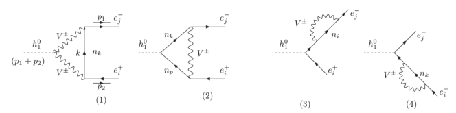
Figure 6: One-loop diagrams contributing to the SM-like Higgs boson decay $h^{0}_{1}\to e_{i}e_{j}$ in the unitary gauge, $V^{\pm}=W^{\pm},Y^{\pm}$.

The decay width for the process $h_{1}^{0}\rightarrow e_{i}e_{j}$ is given by:

$$\Gamma(h_{1}^{0}\rightarrow e_{i}e_{j})\equiv\Gamma(h_{1}^{0}\rightarrow e_{i}^{-}e_{j}^{+})+\Gamma(h^{0}_{1}\rightarrow e_{i}^{+}e_{j}^{-})=\frac{m_{h^{0}_{1}}}{8\pi}\left(|\Delta_{(ij)L}|^{2}+|\Delta_{(ij)R}|^{2}\right),$$ (106)

with the condition $m_{h_{1}^{0}}\gg m_{i,j}$ being $m_{i,j}$ the charged lepton masses.

The corresponding branching ratio is

$${\mathrm{B}r}(h^{0}_{1}\rightarrow e_{i}e_{j})=\Gamma(h_{1}^{0}\rightarrow e_{i}e_{j})/\Gamma^{\mathrm{total}}_{h_{1}^{0}}$$ (107)

where $\Gamma^{\mathrm{total}}_{h_{1}^{0}}\simeq 4.1\times 10^{-3}$ GeV [175]. We define the $\Delta_{(ij)L,R}$ functions

$$\Delta_{(ij)L,R}=\sum_{i=1}^{4}\left(\Delta^{(i)W}_{(ij)L,R}+\Delta^{(i)Y}_{(ij)L,R}\right),$$ (108)

where analytic forms for the functions in the r.h.s. are shown in Appendix C (for detailed calculations, see Refs. [161, 32]). The above formulas were crosschecked using FORM [176, 177].

Numerical input parameters we use for the analysis of the LFV processes correspond to the benchmark point given in Eq. (70), which implies that the corresponding values of the physical observables of the lepton sector are automatically consistent with the neutrino oscillation experimental data. The mixing matrix of the charged lepton sector is fixed as given in Eq. (79). The neutrino mixing matrix $U_{\nu}$ and neutrino masses can be numerically determined from Eq. (99), by using the numerical parameters given in (70). According to our estimates $M^{(1)}_{\nu}$ is nearly independent of $v_{\chi}$. On the other hand the heavy neutrino masses show significant $v_{\chi}$-dependence, because they get main contributions from $M_{3}$ given in Eq. (54). Furthermore they are nearly degenerate, which implies, $m_{n_{4}}\simeq m_{n_{5}}\simeq...\simeq\,m_{n_{9}}\simeq y^{(L)}_{\chi}\frac{v_{\chi}}{\sqrt{2}}\left(\frac{v_{\sigma}}{\Lambda}\right)$ as indicated by Eqs. (60) and (61). Hence we can see the dependence of the LFV branching ratios on the heavy neutrino masses, which are related to $v_{\chi}$ as shown by Eqs. (60), (61) and (54). Besides the two VEVs $v_{\phi}$ and $v_{\rho}$ that were fixed in the discussion of the charged lepton sector, we choose $v_{\xi}=v_{\sigma}=v_{\phi}=\lambda\Lambda$, while the three factors in front of the matrices $M_{1,2,3}$ in Eq. (54) can be written in terms of $y_{1,2}$ as follows

$$y_{1}v_{\eta}\lambda^{16} \equiv\frac{v_{\eta}v_{\chi}v_{\zeta}}{2\sqrt{2}\Lambda^{2}}\left(\frac{v_{\sigma}}{\Lambda}\right)^{11},\quad y_{1\eta}^{(L)}\frac{v_{\eta}v_{\xi}}{\sqrt{6}\Lambda}\left(\frac{v_{\sigma}}{\Lambda}\right)\equiv y_{2}v_{\eta}\lambda^{2},\quad y_{\chi}^{(L)}\frac{v_{\chi}}{\sqrt{2}}\left(\frac{v_{\sigma}}{\Lambda}\right)=\frac{y_{1}y_{2}v^{2}_{\eta}\lambda^{18}}{m_{\nu}},$$ (109)

where $y_{1,2}\sim\mathcal{O}(1)$. In our numerical analysis we fix $\Lambda\simeq 96$ TeV, and the CP-even neutral Higgs mixing parameters are set as follows $s_{\alpha}=0$, $c_{\alpha}=1$. In addition, we consider values for the $Z^{\prime}$ mass satisfying $M_{Z^{\prime}}>4$ TeV, which correspond to a $SU(3)_{L}\times U(1)_{X}$ symmetry breaking scale fulfilling $v_{\chi}>10$ TeV, as derived from the approximate formula $M^{2}_{Z^{\prime}}\simeq g^{2}c^{2}_{W}v^{2}_{\chi}/(3-4s^{2}_{W})$ [131]. Numerical results for Br$(e_{i}\rightarrow e_{j}\gamma)$ and Br$(h^{0}_{1}\rightarrow e_{i}e_{j})$ depending on $y_{1}$ and $y_{2}$ are illustrated in Table 5 for $v_{\chi}=15$ TeV. For $v_{\chi}$ around this value, all numerical results are the same hence it is unnecessary to discuss them here.

$(y_{1},y_{2})$	$m_{n_{4}}$ [GeV]	Br$(\mu\rightarrow e\gamma)$	Br$(\tau\rightarrow e\gamma)$	Br$(\tau\rightarrow\mu\gamma)$	Br$(h^{0}_{1}\rightarrow\mu\,e)$	Br$(h^{0}_{1}\rightarrow\tau\,e)$	Br$(h^{0}_{1}\rightarrow\tau\mu)$
$(0.1,0.1)$	$81.4$	$2.8\times 10^{-13}$	$8.5\times 10^{-14}$	$6.8\times 10^{-13}$	$3.1\times 10^{-18}$	$4.4\times 10^{-13}$	$3.6\times 10^{-12}$
$(0.5,0.1)$	$407$	$4.3\times 10^{-15}$	$1.3\times 10^{-15}$	$1.1\times 10^{-14}$	$9.6\times 10^{-20}$	$1.3\times 10^{-14}$	$1.1\times 10^{-13}$
$(2,0.1)$	$1627.8$	$2.5\times 10^{-17}$	$7.8\times 10^{-18}$	$6.2\times 10^{-17}$	$1.2\times 10^{-19}$	$1.6\times 10^{-14}$	$1.3\times 10^{-13}$
$(5,0.1)$	$4069.5$	$6.8\times 10^{-19}$	$2.1\times 10^{-19}$	$1.7\times 10^{-18}$	$8.3\times 10^{-19}$	$1.2\times 10^{-13}$	$9.5\times 10^{-13}$
$(0.1,0.5)$	$4.1\times 10^{2}$	$2.7\times 10^{-12}$	$8.2\times 10^{-13}$	$6.6\times 10^{-12}$	$6.1\times 10^{-17}$	$8.5\times 10^{-12}$	$7.0\times 10^{-11}$
$(0.5,0.5)$	$2.03\times 10^{3}$	$6.6\times 10^{-15}$	$2.0\times 10^{-15}$	$1.6\times 10^{-14}$	$1.2\times 10^{-16}$	$1.6\times 10^{-11}$	$1.4\times 10^{-10}$
$(2,0.5)$	$8.14\times 10^{3}$	$2.7\times 10^{-17}$	$8.2\times 10^{-18}$	$6.6\times 10^{-17}$	$1.6\times 10^{-15}$	$2.3\times 10^{-10}$	$1.9\times 10^{-9}$
$(0.1,2)$	$1.63\times 10^{3}$	$4.1\times 10^{-12}$	$1.2\times 10^{-12}$	$9.9\times 10^{-12}$	$1.9\times 10^{-14}$	$2.6\times 10^{-9}$	$2.2\times 10^{-8}$
$(0.5,2)$	$8.14\times 10^{3}$	$6.9\times 10^{-15}$	$2.1\times 10^{-15}$	$1.7\times 10^{-14}$	$4.1\times 10^{-13}$	$5.8\times 10^{-8}$	$4.8\times 10^{-7}$
$(0.1,4.5)$	$3.66\times 10^{3}$	$4.2\times 10^{-12}$	$1.3\times 10^{-12}$	$1.0\times 10^{-11}$	$2.8\times 10^{-12}$	$3.9\times 10^{-7}$	$3.2\times 10^{-6}$
$(0.2,\;4.5)$	$7325.4$	$2.7\times 10^{-13}$	$8.2\times 10^{-14}$	$6.6\times 10^{-13}$	$9.2\times 10^{-12}$	$1.3\times 10^{-6}$	$1.1\times 10^{-5}$

Table 5: Branching ratios for the LFV decays with $v_{\chi}=15$ TeV. The second column presents the numerical values of the heavy neutrino masses.

The product $y_{1}y_{2}$ is constrained by the perturbative limit of the Yukawa coupling $y_{1}y_{2}\sim y^{L}_{\chi}<\sqrt{4\pi}\simeq 3.5$, as follows from Eq. (109). Table 5 shows the numerical values of the Branching ratios for the LFV decays with $v_{\chi}=15$ TeV and different values of the Yukawa couplings $y_{1}$ and $y_{2}$ and heavy neutrino masses. Notice that a specific value of $(y_{1},y_{2})$ in Table 5, will predict a value for the Yukawa coupling $y^{L}_{\chi}\simeq\sqrt{2}m_{n_{4}}/(v_{\chi}\lambda)\leq 3.5$, leading to $m_{n_{4}}\leq 0.557v_{\chi}$. Thus for $v_{\chi}=15$ TeV we have $m_{n_{4}}\leq 8.35$ TeV.

Based on the numerical results reported in Table 5, we can see that Br$(\mu\rightarrow\,e\gamma)$ can reach values close to its recent experimental bound provided that $y_{1}$ is small enough. On the other hand, Br$(h^{0}_{1}\rightarrow\mu\tau)$ can reach $\mathcal{O}(10^{-5})$ values when $y_{2}$ is large enough, like for example $y_{2}=4.5$ as shown in Table 5. Furthermore, increasing $y_{2}$ will result in larger values for Br$(h^{0}_{1}\rightarrow\mu\tau)$. We can see that the Br$(h^{0}_{1}\rightarrow e_{i}e_{j})$ is enhanced when the heavy neutrino mass $m_{n_{4}}$ is increased, which is a generic behavior observed in inverse seesaw models [160, 161]. Because the experiment data favors lower bounds of $y_{1}$, and the perturbative limit of $y^{L}_{\chi}$ and $v_{\chi}$ results in upper bounds of $y_{2}$, there exist upper bounds, which are order of $\mathcal{O}(10^{-5})$ and $\mathcal{O}(10^{-6})$ for the Branching ratios of the two decays $h^{0}_{1}\rightarrow\mu\tau,e\tau$ for the numerical values of the free parameters chosen above. The remaining LFV decays $\tau\rightarrow\mu\gamma,e\gamma$ and $h^{0}_{1}\rightarrow e\mu$ have much smaller Branching ratios than the characteristic sensitivities of current experimental searches.

VIII Conclusions

We constructed a viable multiscalar singlet extension of the 3-3-1 model with two scalar triplets and three right handed Majorana neutrinos where the tiny masses for the light active neutrinos are produced by the linear seesaw mechanism. Our model is based on the $A_{4}$ family symmetry, which is supplemented by other auxiliary symmetries. The observed pattern of the SM charged fermion masses and fermionic mixing parameters originates from the spontaneous breaking of the discrete symmetries of the model and does not require any fine-tuning of the model parameters.

We analyzed the implications of our model in the lepton flavour violating processes. We demonstrated that the branching ratio Br$(\mu\rightarrow\,e\gamma)$ can reach values close to the recent upper experimental bounds, thus constraining the values of Br$(\tau\rightarrow\mu\gamma)$ and Br$(\tau\rightarrow e\gamma)$ to be much smaller than the corresponding experimental sensitivities. On the other hand, the model allows Br$(h^{0}_{1}\rightarrow\mu\tau)$ and Br$(h^{0}_{1}\rightarrow\,e\tau)$ to reach the values of about $\mathcal{O}(10^{-5})$ and $\mathcal{O}(10^{-6})$, respectively. Besides that, we have studied the implications of our model in meson oscillations and we have found that our model is consistent with the constraints arising from meson mixings. We also studied the production of the heavy $Z^{\prime}$ gauge boson in proton-proton collisions via the Drell-Yan mechanism. We found that the corresponding total cross section ranges at the LHC from $0.11$ fb up to $0.01$ fb when the $Z^{\prime}$ gauge boson mass is varied within $7-8$ TeV interval. The $Z^{\prime}$ production cross section will be significantly enhanced at the proposed energy upgrade of the LHC with $\sqrt{S}=28$ TeV reaching typical values of $82-30$ fb. From these results we found that the $pp\to Z^{\prime}\to l^{+}l^{-}$ resonant production cross section reach the values of about $10^{-3}$ fb and $1$ fb for $M_{Z^{\prime}}=7$ TeV at the energies $\sqrt{s}=13$ TeV and $\sqrt{s}=28$ TeV, respectively.

The first value of the resonant production cross section is below and the second lies on the verge of the sensitivities of the LHC experiments at the corresponding energies.

Appendix A The product rules for $A_{4}$

The $A_{4}$ group has one three-dimensional $\mathbf{3}$ and three distinct one-dimensional $\mathbf{1}$, $\mathbf{1}^{\prime}$ and $\mathbf{1}^{\prime\prime}$ irreducible representations, satisfying the following product rules:

$$\hskip 51.21495pt\mathbf{3}\otimes\mathbf{3}=\mathbf{3}_{s}\oplus\mathbf{3}_{a}\oplus\mathbf{1}\oplus\mathbf{1}^{\prime}\oplus\mathbf{1}^{\prime\prime},$$ (110)

$$\mathbf{1}\otimes\mathbf{1}=\mathbf{1},\hskip 14.22636pt\mathbf{1}^{\prime}\otimes\mathbf{1}^{\prime\prime}=\mathbf{1},\hskip 14.22636pt\mathbf{1}^{\prime}\otimes\mathbf{1}^{\prime}=\mathbf{1}^{\prime\prime},\hskip 14.22636pt\mathbf{1}^{\prime\prime}\otimes\mathbf{1}^{\prime\prime}=\mathbf{1}^{\prime},$$

Considering $\left(x_{1},x_{2},x_{3}\right)$ and $\left(y_{1},y_{2},y_{3}\right)$ as the basis vectors for two $A_{4}$-triplets $\mathbf{3}$, the following relations are fulfilled:

$$\left(\mathbf{3}\otimes\mathbf{3}\right)_{\mathbf{1}}=x_{1}y_{1}+x_{2}y_{2}+x_{3}y_{3},$$ (111)

$$\left(\mathbf{3}\otimes\mathbf{3}\right)_{\mathbf{3}_{s}}=\left(x_{2}y_{3}+x_{3}y_{2},x_{3}y_{1}+x_{1}y_{3},x_{1}y_{2}+x_{2}y_{1}\right),\ \ \ \ \left(\mathbf{3}\otimes\mathbf{3}\right)_{\mathbf{1}^{\prime}}=x_{1}y_{1}+\omega x_{2}y_{2}+\omega^{2}x_{3}y_{3},$$

$$\left(\mathbf{3}\otimes\mathbf{3}\right)_{\mathbf{3}_{a}}=\left(x_{2}y_{3}-x_{3}y_{2},x_{3}y_{1}-x_{1}y_{3},x_{1}y_{2}-x_{2}y_{1}\right),\ \ \ \left(\mathbf{3}\otimes\mathbf{3}\right)_{\mathbf{1}^{\prime\prime}}=x_{1}y_{1}+\omega^{2}x_{2}y_{2}+\omega x_{3}y_{3},$$

where $\omega=e^{i\frac{2\pi}{3}}$. The representation $\mathbf{1}$ is trivial, while the non-trivial $\mathbf{1}^{\prime}$ and $\mathbf{1}^{\prime\prime}$ are complex conjugate to each other. Some reviews of discrete symmetries in particle physics are found in Refs. [178, 179, 180, 181]. The discrete symmetry $A_{4}$ was first implemented to the 3-3-1 models in the Refs [182] and [11].

Appendix B Scalar sector

Here we present more details about the scalar sector of our model containing the SM Higgs boson.

The scalar potential of the model can be splitted in the following two parts:

$$V_{S}=V^{\mathrm{invariant}}_{S}+V^{\mathrm{soft}}_{S}.$$ (112)

The first part $V^{\mathrm{invariant}}_{S}$ is invariant under the $A_{4}\times Z_{8}\times Z_{14}\times Z_{22}$ discrete and $SU(3)_{C}\times SU(3)_{L}\times U(1)_{X}$ gauge symmetries,

$$V^{\mathrm{invariant}}_{S} =\mu_{\chi}^{2}\chi^{\dagger}\chi+\mu_{\eta}^{2}\eta^{\dagger}\eta+\mu_{\sigma}^{2}\sigma^{*}\sigma+\mu_{\xi}^{2}(\xi^{*}\xi)_{1}+\mu_{\zeta}^{2}(\zeta^{*}\zeta)_{1}+\mu_{\rho}^{2}(\rho^{*}\rho)_{1}+\mu_{\varphi}^{2}(\varphi^{*}\varphi)_{1}+\mu_{\phi}^{2}(\phi^{*}\phi)_{1}+\left[\mu_{\phi\rho}^{2}(\phi^{*}\rho)_{1}+\mathrm{H.c.}\right]$$

$$+\lambda_{\chi}(\chi^{\dagger}\chi)^{2}+\lambda_{\eta}(\eta^{\dagger}\eta)^{2}+\lambda_{\sigma}(\sigma^{*}\sigma)^{2}+\sum_{S_{i},S_{j}}\left[(S_{i}^{*}S_{i})(S_{j}^{*}S_{j})\right]_{1}$$

$$+\lambda_{\chi\eta}(\chi^{\dagger}\chi)(\eta^{\dagger}\eta)+\lambda^{\prime}_{\chi\eta}(\chi^{\dagger}\eta)(\eta^{\dagger}\chi)+(\sigma^{\ast}\sigma)\left[\lambda_{\chi\sigma}(\chi^{\dagger}\chi)+\lambda_{\eta\sigma}(\eta^{\dagger}\eta)\right]$$

$$+\left\{\left[(\rho\rho)(\phi^{*}\phi^{*})\right]_{1}+\left[(\xi\rho)(\varphi^{*}\varphi^{*})\right]_{1}+\left[(\xi\phi)(\varphi^{*}\varphi^{*})\right]_{1}+\mathrm{H.c.}\right\}$$

$$+(\sigma^{\ast}\sigma)\left\{\sum_{S}\lambda_{S\sigma}(S^{*}S)_{1}+\left[\lambda_{\phi\rho\sigma}(\phi^{*}\rho)_{1}+\mathrm{H.c.}\right]\right\}$$

$$+(\chi^{\dagger}\chi)\left\{\sum_{S}\lambda_{S\chi}(S^{*}S)_{1}+\left[\lambda_{\phi\rho\chi}(\phi^{*}\rho)_{1}+\mathrm{H.c.}\right]\right\}$$

$$+(\eta^{\dagger}\eta)\sum_{S}\lambda_{S\eta}(S^{*}S)_{1}+\left[\lambda_{\phi\rho\eta}(\phi^{*}\rho)_{1}+\mathrm{H.c.}\right]$$

$$+\sum_{S}\left\{\left[(\phi^{*}\rho)(S^{*}S)\right]_{1}+\mathrm{H.c.}\right\},$$ (113)

where $S,S_{i},S_{j}=\xi,\zeta,\rho,\varphi,\phi$ are the scalar fields defined in Eq. (II). The second part $V^{\mathrm{soft}}_{S}$ consists of $A_{4}\times Z_{8}\times Z_{14}\times Z_{22}$ soft-breaking terms needed to generate non-zero masses for the CP-odd neutral Higgs bosons as well as to solve the domain wall problem. The complete set of these soft-breaking terms is

$$V^{\mathrm{soft}}_{S} =\mu^{\prime 2}_{\sigma}\sigma^{2}+f_{\sigma}\sigma^{3}+\sum_{S}\left[\mu^{2}_{1^{\prime},S}\left(S^{2}\right)_{1^{\prime}}+f_{S}\left(S^{2}\right)_{1}\sigma\right]+\mathrm{H.c.},$$ (114)

where $S=\xi,\zeta,\rho,\varphi,\phi$; all parameters $\mu^{\prime}_{\sigma}$, $f_{\sigma}$, $\mu^{2}_{1^{\prime},S}$, and $f_{S}$ have the same dimension of mass.

The $A_{4}$-invariant products of four $A_{4}$-triplets $x,y,z,t$ can be decomposed as:

$$\left[(xy)(zt)\right]_{1} \equiv\lambda^{xyzt}_{1}(xy)_{1}(zt)_{1}+\lambda^{xyzt}_{2}(xy)_{1^{\prime}}(zt)_{1^{\prime\prime}}+\lambda^{xyzt}_{3}(xy)_{1^{\prime\prime}}(zt)_{1^{\prime}}+\lambda^{xyzt}_{4}\left[(xy)_{3s}(zt)_{3s}\right]_{1}$$

$$+\lambda^{xyzt}_{5}\left[(xy)_{3s}(zt)_{3a}\right]_{1}+\lambda^{xyzt}_{6}\left[(xy)_{3a}(zt)_{3s}\right]_{1}+\lambda^{xyzt}_{7}\left[(xy)_{3a}(zt)_{3a}\right]_{1}.$$ (115)

The products like $\left[(xz)(yt)\right]_{1}$, $\left[(xt)(yz)\right]_{1}$,… are not included in the scalar potential (113) because they can always be written as linear combinations of the seven $A_{4}$-products in the right hand side of Eq. (B). This fact can be easily demonstrated, using the rules given in Appendix A. Let us note that due to the antisymmetry and symmetry properties of the $3_{a}$ and $3_{s}$ triplet components in the products $(\xi\xi)$ and $(\zeta\zeta)$, we obtain $(3_{s}3_{a})_{1}+\mathrm{H.c.}=0$. Hence many terms of this kind does not appear in the scalar potential. Therefore, particular cases are written as

$$\left[(S^{*}S)^{2}\right]_{1} \equiv\lambda^{S}_{1}(S^{*}S)_{1}(S^{*}S)_{1}+\lambda^{S}_{2}(S^{*}S)_{1^{\prime}}(S^{*}S)_{1^{\prime\prime}}+\lambda^{S}_{4}\left[(S^{*}S)_{3_{s}}(S^{*}S)_{3_{s}}\right]_{1}+\lambda^{S}_{7}\left[(S^{*}S)_{3_{a}}(S^{*}S)_{3_{a}}\right]_{1},$$

$$\left[S_{i}^{*}S_{i}S_{j}^{*}S_{j}\right]_{1} \equiv\lambda^{S_{i}S_{j}}_{1}(S_{i}^{*}S_{i})_{1}(S_{j}^{*}S_{j})_{1}+\left[\lambda^{S_{i}S_{j}}_{2}(S_{i}^{*}S_{i})_{1^{\prime}}(S_{j}^{*}S_{j})_{1^{\prime\prime}}+\mathrm{H.c.}\right]+\lambda^{S_{i}S_{j}}_{4}(S_{i}^{*}S_{i})_{3_{s}}(S_{j}^{*}S_{j})_{3_{s}}$$

$$+\lambda^{S_{i}S_{j}}_{7}(S_{i}^{*}S_{i})_{3_{a}}(S_{j}^{*}S_{j})_{3_{a}},\hskip 8.5359ptS_{i}\neq S_{j},$$

$$\left[(\xi\xi)(\varphi^{*}\varphi^{*})\right]_{1} =\lambda^{\prime\xi\varphi}_{1}(\xi\xi)_{1}(\varphi^{*}\varphi^{*})_{1}+\lambda^{\prime\xi\varphi}_{2}(\xi\xi)_{1^{\prime}}(\varphi^{*}\varphi^{*})_{1^{\prime\prime}}+\lambda^{\prime\xi\varphi}_{3}(\xi\xi)_{1^{\prime\prime}}(\varphi^{*}\varphi^{*})_{1^{\prime}}+\lambda^{\prime\xi\varphi}_{4}\left[(\xi\xi)_{3s}(\varphi^{*}\varphi^{*})_{3s}\right]_{1},$$

$$\left[(\rho\rho)(\phi^{*}\phi^{*})\right]_{1} =\lambda^{\prime\rho\phi}_{1}(\rho\rho)_{1}(\phi^{*}\phi^{*})_{1}+\lambda^{\prime\rho\phi}_{2}(\rho\rho)_{1^{\prime}}(\phi^{*}\phi^{*})_{1^{\prime\prime}}+\lambda^{\prime\rho\phi}_{3}(\rho\rho)_{1^{\prime\prime}}(\phi^{*}\phi^{*})_{1^{\prime}}+\lambda^{\prime\rho\phi}_{4}\left[(\rho\rho)_{3s}(\phi^{*}\phi^{*})_{3s}\right]_{1},$$

$$\left[(\xi\varphi^{*})(\rho\phi^{*})\right]_{1} =\lambda^{\xi\varphi\rho\phi^{*}}_{1}(\xi\varphi^{*})_{1}(\rho\phi^{*})_{1}+\lambda^{\xi\varphi\rho\phi^{*}}_{2}(\xi\varphi^{*})_{1^{\prime}}(\rho\phi^{*})_{1^{\prime\prime}}+\lambda^{\xi\varphi\rho\phi^{*}}_{3}(\xi\varphi^{*})_{1^{\prime\prime}}(\rho\phi^{*})_{1^{\prime}}+\lambda^{\xi\varphi\rho\phi^{*}}_{4}\left[(\xi\varphi^{*})_{3s}(\rho\phi^{*})_{3s}\right]_{1}$$

$$+\lambda^{\xi\varphi\rho\phi^{*}}_{5}\left[(\xi\varphi^{*})_{3s}(\rho\phi^{*})_{3a}\right]_{1}+\lambda^{\xi\varphi\rho\phi^{*}}_{6}\left[(\xi\varphi^{*})_{3a}(\rho\phi^{*})_{3s}\right]_{1}+\lambda^{\xi\varphi\rho\phi^{*}}_{7}\left[(\xi\varphi^{*})_{3a}(\rho\phi^{*})_{3a}\right]_{1},$$

$$\left[(\xi\varphi^{*})(\rho^{*}\phi)\right]_{1} =\lambda^{\xi\varphi\rho^{*}\phi}_{1}(\xi\varphi^{*})_{1}(\rho^{*}\phi)_{1}+\lambda^{\xi\varphi\rho^{*}\phi}_{2}(\xi\varphi^{*})_{1^{\prime}}(\rho^{*}\phi)_{1^{\prime\prime}}+\lambda^{\xi\varphi\rho^{*}\phi}_{3}(\xi\varphi^{*})_{1^{\prime\prime}}(\rho^{*}\phi)_{1^{\prime}}+\lambda^{\xi\varphi\rho^{*}\phi}_{4}\left[(\xi\varphi^{*})_{3s}(\rho^{*}\phi)_{3s}\right]_{1}$$

$$+\lambda^{\xi\varphi\rho^{*}\phi}_{5}\left[(\xi\varphi^{*})_{3s}(\rho^{*}\phi)_{3a}\right]_{1}+\lambda^{\xi\varphi\rho^{*}\phi}_{6}\left[(\xi\varphi^{*})_{3a}(\rho^{*}\phi)_{3s}\right]_{1}+\lambda^{\xi\varphi\rho^{*}\phi}_{7}\left[(\xi\varphi^{*})_{3a}(\rho^{*}\phi)_{3a}\right]_{1}.$$ (116)

The above scalar potential has a fairly large number of scalar self-interactions.

The VEV’s chosen in Eq. (16) must satisfy all the minimization conditions of the scalar potential (113), namely

$$\left.\frac{\partial\,V_{H}}{\partial\,S^{0}}\right|_{S^{0}=\langle S^{0}\rangle,\forall\,S^{0}}=0.$$ (117)

The model contains 20 neutral scalar components, where three of them have zero VEVs. This leads to 20 minimization equations relating the VEVs to the parameters of the scalar potential. We find that two equations for $\chi^{0}_{1}$ and $\rho^{0}_{3}$ are automatically satisfied. The remaining 18 equations allow expressing 18 parameters of the model in terms of the other ones.

In order to generate fermions masses consistent with experiments we introduced in (20) the VEV pattern implying new relations between VEVs. Let us show that this pattern is consistent with the scalar potential (113). It suffices to consider the simplified case of the scalar potential in the decoupling limit, when the quartic couplings of the scalar $SU(3)_{L}$-triplets vanish, with the exception of two $SU(3)_{L}$-triples. We will comment on more general cases later. The minimization conditions for the neutral scalars with real vev’s take in the decoupling limit the form

$$S^{0}=\chi^{0}_{3}\rightarrow\mu_{\chi}^{2} =-\frac{\lambda_{\chi\eta}v_{\eta}^{2}}{2}-\lambda_{\chi}v_{\chi}^{2},$$

$$S^{0}=\eta^{0}_{1}\rightarrow\mu_{\eta}^{2} =-\frac{\lambda_{\chi\eta}v_{\chi}^{2}}{2}-\lambda_{\eta}v_{\eta}^{2},$$

$$S^{0}=\sigma^{0}\rightarrow\mu_{\sigma}^{2} =-v_{\sigma}^{2}\lambda_{\sigma}-2\mu^{\prime 2}_{\sigma}-\frac{3f_{\sigma}v_{\sigma}}{\sqrt{2}}-\frac{\sqrt{2}\left(f_{\zeta}v_{\zeta}^{2}+f_{\xi}v_{\xi}^{2}+f_{\rho}v_{\rho}^{2}\right)}{v_{\sigma}}$$

$$\quad-\frac{\sqrt{2}f_{\phi}v_{\phi}^{2}e^{i\psi}s_{2\alpha}}{v_{\sigma}}+\frac{\sqrt{2}f_{\varphi}v_{\varphi}^{2}e^{-i\psi}s_{2\alpha}}{v_{\sigma}},$$

$$S^{0}=\xi_{1}^{0},\xi_{2}^{0},\xi_{3}^{0}\rightarrow\mu_{\xi}^{2} =-\sqrt{2}f_{\xi}v_{\sigma}-\frac{2}{3}v_{\xi}^{2}(3\lambda_{1}^{\xi}+4\lambda_{4}^{\xi}),$$

$$\mu_{1^{\prime}\xi}^{2} =0,$$

$$S^{0}=\zeta_{1}^{0},\zeta_{3}^{0}\rightarrow\mu_{\zeta}^{2} =-\sqrt{2}f_{\zeta}v_{\sigma}-v_{\zeta}^{2}(2\lambda_{1}^{\zeta}+\lambda_{3}^{\zeta}+2\lambda_{4}^{\zeta}),$$

$$\mu_{1^{\prime}\zeta}^{2} =-\frac{v_{\zeta}^{2}(2w+1)(\lambda_{2}^{\zeta}-\lambda_{3}^{\zeta})}{2(w+2)},$$

$$S^{0}=\rho_{1}^{0},\rho_{2}^{0},\rho_{3}^{0}\rightarrow\mu_{\rho}^{2} =-\frac{2}{3}v_{\rho}^{2}(3\lambda_{1}^{\rho}+4\lambda_{4}^{\rho}),$$

$$\mu_{\phi\rho}^{2} =0,\;\mu_{1^{\prime}\rho}^{2}=0,$$ (118)

where we have used that $\sum_{i=1}^{3}\langle\phi_{i}\rangle^{2}=v_{\phi}^{2}e^{i\psi}s_{2\alpha}$ and $\sum_{i=1}^{3}\langle\varphi_{i}\rangle^{2}=-v_{\varphi}^{2}e^{-i\psi}s_{2\alpha}$.

Next, we consider the $A_{4}$-triplets $\phi$ and $\varphi$ with complex VEVs given in Eq. (16). With $\mu_{\phi\rho}=0$, we have three different minimization equations for $\phi$ in the following forms:

$$S^{0}=\phi^{0}_{1}\rightarrow 0= \frac{3x_{1}^{2}\mu_{\phi}^{2}}{2v_{\phi}^{2}}+\lambda_{1}^{\phi}\left(x_{1}^{2}+x_{2}^{2}+x_{3}^{2}\right)+\lambda_{2}^{\phi}\left(2x_{1}^{2}-x_{2}^{2}-x_{3}^{2}\right)+4x_{1}^{2}\lambda_{4}^{\phi}+\frac{3\mu_{1^{\prime}\phi}^{2}}{v_{\phi}^{2}}+\frac{3f_{\phi}v_{\sigma}}{\sqrt{2}v_{\phi}^{2}},$$

$$S^{0}=\phi^{0}_{2}\rightarrow 0= \frac{3x_{2}^{2}\mu_{\phi}^{2}}{2v_{\phi}^{2}}+\lambda_{1}^{\phi}\left(x_{1}^{2}+x_{2}^{2}+x_{3}^{2}\right)+\lambda_{2}^{\phi}\left(-x_{1}^{2}+2x_{2}^{2}-x_{3}^{2}\right)+4x_{2}^{2}\lambda_{4}^{\phi}+\frac{3w\mu_{1^{\prime}\phi}^{2}}{v_{\phi}^{2}}+\frac{3f_{\phi}v_{\sigma}}{\sqrt{2}v_{\phi}^{2}},$$

$$S^{0}=\phi^{0}_{3}\rightarrow 0= \frac{3x_{3}^{2}\mu_{\phi}^{2}}{2v_{\phi}^{2}}+\lambda_{1}^{\phi}\left(x_{1}^{2}+x_{2}^{2}+x_{3}^{2}\right)+\lambda_{2}^{\phi}\left(-x_{1}^{2}-x_{2}^{2}+2x_{3}2\right)+4x_{3}^{2}\lambda_{4}^{\phi}+\frac{3w^{2}\mu_{1^{\prime}\phi}^{2}}{v_{\phi}^{2}}+\frac{3f_{\phi}v_{\sigma}}{\sqrt{2}v_{\phi}^{2}},$$ (119)

where $x_{1}=c_{\alpha}+e^{i\psi}s_{\alpha}$, $x_{2}=w\left(c_{\alpha}+we^{i\psi}s_{\alpha}\right)$, and $x_{3}=w^{2}\left(c_{\alpha}+w^{2}e^{i\psi}s_{\alpha}\right)$ that satisfy $x_{1}+x_{2}+x_{3}=0$. Other relations used in our calculation are: $\sum_{i=1}^{3}x_{i}^{2}=6c_{\alpha}s_{\alpha}e^{i\psi}$. From the scalar potential minimization equations we find:

$$\mu_{\phi}^{2} =-\frac{2}{3}v_{\phi}^{2}(3\lambda_{1}^{\phi}+4\lambda_{4}^{\phi})-\frac{3\sqrt{2}f_{\phi}v_{\sigma}}{x_{1}^{2}+x_{2}^{2}+x_{3}^{2}},\ \mu_{1^{\prime}\phi}^{2}=0,$$

$$\lambda_{2}^{\phi} =\lambda_{1}^{\phi}+\frac{3f_{\phi}v_{\sigma}}{\sqrt{2}v_{\phi}^{2}\left(x_{1}^{2}+x_{2}^{2}+x_{3}^{2}\right)}.$$ (120)

In the same way, we treat the minimization conditions for $\varphi$ and find the following relations

$$\mu_{\varphi}^{2} =-\frac{2}{3}v_{\varphi}^{2}(3\lambda_{1}^{\varphi}+4\lambda_{4}^{\varphi})-\frac{3\sqrt{2}f_{\varphi}v_{\sigma}}{y_{1}^{2}+y_{2}^{2}+y_{3}^{2}},\;\mu_{1^{\prime}\varphi}^{2}=0,$$

$$\lambda_{2}^{\varphi} =\lambda_{1}^{\varphi}+\frac{3f_{\varphi}v_{\sigma}}{\sqrt{2}v_{\varphi}^{2}\left(y_{1}^{2}+y_{2}^{2}+y_{3}^{2}\right)},$$ (121)

where $y_{1}=c_{\alpha}-e^{-i\psi}s_{\alpha}$, $y_{2}=w^{2}\left(c_{\alpha}-w^{2}e^{-i\psi}s_{\alpha}\right)$, and $y_{3}=w\left(c_{\alpha}-we^{-i\psi}s_{\alpha}\right)$.

Thus, we see that the minimization conditions in the decoupling limit do not constrain the vev’s. This conclusion is valid in the general case, when all the quartic coupling return back to the scalar potential. This is trivially because these couplings just introduce new independent parameters, which can not introduce any constraint on the vev’s.

Let us identify the SM-like Higgs boson with one of the scalars of our model or their linear combination.

Note that the neutral CP-even components of the Higgs bosons always contain only one massless state absorbed by the gauge boson $X^{0}$. This state is one of the linear combinations of the two real components $R(\chi^{0}_{1})$ and $R(\eta^{0}_{3})$, which have zero VEVs. More precisely, the model contains two would-be Goldstone bosons $G_{X},G^{*}_{X}$, a neutral CP-odd Higgs boson $h_{a}$, and a mass eigenstate $h^{0}_{3}$. Namely, defining

$$t_{\theta}=\tan\theta=\frac{v_{\eta}}{v_{\chi}},$$

we have the following relations between the original and the mass eigenstates of the neutral Higgs bosons

$$\begin{pmatrix}R_{\chi_{1}}\\ R_{\eta_{3}}\end{pmatrix} =\begin{pmatrix}c_{\theta}&s_{\theta}\\ -s_{\theta}&c_{\theta}\end{pmatrix}\begin{pmatrix}G_{X}\\ h^{0}_{3}\end{pmatrix},\;\begin{pmatrix}I_{\chi_{1}}\\ I_{\eta_{3}}\end{pmatrix}=\begin{pmatrix}c_{\theta}&s_{\theta}\\ -s_{\theta}&c_{\theta}\end{pmatrix}\begin{pmatrix}\overline{G}_{X}\\ h_{a}\end{pmatrix},$$

$$m_{G_{X}} =m_{\overline{G}_{X}}=0,\quad m^{2}_{h^{0}_{3}}=m^{2}_{h_{a}}=\frac{1}{2}\lambda^{\prime}_{\eta\chi}(v^{2}_{\eta}+v^{2}_{\chi}).$$ (122)

The $R_{\zeta_{2}}$ is one mass eigenstate with mass $m^{2}_{R_{\zeta_{2}}}=\frac{2}{9}(-3\lambda)v_{\zeta}^{2}$.

The remaining CP-even components of the neutral Higgs boson consist of 17 states $\xi_{\chi}=\sqrt{2}R_{\chi^{0}_{3}}$, $\xi_{\eta}=\sqrt{2}R_{\eta^{0}_{1}}$, $R_{\sigma}$, $R_{\xi_{i}}$ ($i=1,2,3$), $R_{\zeta_{1}}$, and $R_{\zeta_{3}}$. The squared mass matrix of these states is the $17\times 17$ matrix denoted as $\mathcal{M}^{2}_{h}$. This matrix has non-zero determinant, which means that all the neutral CP-even Higgs bosons are massive. In addition, $\mathrm{Det}[\mathcal{M}^{2}_{h}]_{v_{\eta}=0}=0$ implies that there is at least one Higgs boson with mass at the electroweak scale. That lightest CP even scalar state is identified with the SM-like $126$ GeV Higgs boson.

To illustrate that there is one Higgs that can be identified with the $126$ GeV SM-like Higgs boson found by LHC, we consider the simplified case when the $SU(3)_{L}$ triplets $\chi$ and $\eta$ decouple from $S=\sigma$, $\xi_{i}$, $\zeta_{1},\;\zeta_{3}$, $\rho_{i},\;\varphi_{i}$, and $\phi_{i}$ so that the corresponding quartic couplings vanish $\lambda_{\eta S}=\lambda_{\chi S}=0$. Then, the matrix $\mathcal{M}^{2}_{h}$ is split into two block-diagonal $2\times 2$ and $15\times 15$ matrices. The first matrix in the basis $(\xi_{\eta},\;\xi_{\chi})$ takes form

$$\mathcal{M}^{2}_{h1}=\begin{pmatrix}2\lambda_{\eta}v_{\eta}^{2}&\lambda_{\eta\chi}v_{\chi}v_{\eta}\\ \lambda_{\eta\chi}v_{\chi}v_{\eta}&2\lambda_{\chi}v_{\chi}^{2}\end{pmatrix}.$$ (123)

Its mass eigenstates, $h^{0}_{1}$ and $h^{0}_{2}$, and their masses are

$$m^{2}_{h^{0}_{1,2}} =\lambda_{\chi}v_{\chi}^{2}+\lambda_{\eta}v_{\eta}^{2}\mp\sqrt{\left(\lambda_{\chi}v_{\chi}^{2}-\lambda_{\eta}v_{\eta}^{2}\right)^{2}+\lambda_{\eta\chi}^{2}v_{\chi}^{2}v_{\eta}^{2}},$$

$$\begin{pmatrix}\xi_{\eta}\\ \xi_{\chi}\end{pmatrix} =\begin{pmatrix}c_{\alpha}&s_{\alpha}\\ -s_{\alpha}&c_{\alpha}\end{pmatrix}\begin{pmatrix}h^{0}_{1}\\ h^{0}_{2}\end{pmatrix},\quad t_{2\alpha}\equiv\tan(2\alpha)=\frac{\lambda_{\eta\chi}t_{\theta}}{\lambda_{\chi}-\lambda_{\eta}t_{\theta}^{2}}.$$ (124)

These two neutral Higgs bosons are similar in many respects to those discussed in the model [41]. Analogously to this model, in our case in the limit $t_{\theta}\ll 1$, we find that $m^{2}_{h^{0}_{1}}\simeq\left(2\lambda_{\eta}-\frac{\lambda_{\eta\chi}^{2}}{\lambda_{\chi}}\right)v^{2}_{\eta}$, as should be for the SM Higgs boson, the mass of which is generated on the electroweak scale. Thus, we identify $h^{0}_{1}$ with the SM-like Higgs boson found by the LHC. The simplified case when $t_{\theta}\ll 1$ is used in our discussion of the LFV Higgs decays in Sec. VII.

The soft breaking terms introduced in the Higgs potential (114) are enough to generate non-zero masses for all CP-odd Higgs bosons in the model under consideration, even some of them vanish by the minimization conditions of the Higgs potential. Namely, in the limit of $f_{S}=0$ with all $S=\sigma,\xi,\;\zeta,\rho,\;\varphi,\;\phi$, the total squared mass matrix of the CP-odd neutral components in the basis $S_{0}=(I_{\sigma},\;I_{\xi_{i}},\;I_{\zeta_{i}},I_{\rho,_{i}}\;I_{\phi_{i}},\;I_{\varphi_{i}})$ separates into the six block sub-matrices, including one physical state $I_{\sigma}$ and another five $3\times 3$ matrices.

$$m^{2}_{a_{\sigma}} =-4\mu^{\prime 2}_{\sigma},\;$$

$$m^{2}_{\xi_{i}} =\left\{\frac{1}{3}v_{\xi}^{2}(3\lambda_{1}^{\xi}+4\lambda_{4}^{\xi}),\frac{1}{3}v_{\xi}^{2}(-15\lambda_{1}^{\xi}+18\lambda_{2}^{\xi}+4\lambda_{4}^{\xi}),\frac{1}{3}v_{\xi}^{2}(-15\lambda_{1}^{\xi}+18\lambda_{2}^{\xi}+4\lambda_{4}^{\xi})\right\},$$

$$M^{2}_{I_{\zeta}} =\left(\begin{array}[]{ccc}\frac{-3\lambda_{3}^{\zeta}w-4\lambda_{1}^{\zeta}(w+2)+\lambda_{2}^{\zeta}(7w+8)}{2(w+2)}&0&2\lambda_{1}^{\zeta}-\lambda_{2}^{\zeta}-\lambda_{3}^{\zeta}\\ 0&\frac{3\lambda_{2}^{\zeta}+\lambda_{3}^{\zeta}+8\lambda_{4}^{\zeta}+2\lambda_{3}^{\zeta}w+4\lambda_{4}^{\zeta}w-8\lambda_{1}^{\zeta}(w+2)}{2(w+2)}&0\\ 2\lambda_{1}^{\zeta}-\lambda_{2}^{\zeta}-\lambda_{3}^{\zeta}&0&\frac{3\lambda_{3}^{\zeta}(w+1)-4\lambda_{1}^{\zeta}(w+2)+\lambda_{2}^{\zeta}(w+5)}{2(w+2)}\\ \end{array}\right){\color[rgb]{0,0,1}v_{\zeta}^{2}},$$ (128)

$$m^{2}_{a_{\rho_{i}}} =\frac{v_{\rho^{2}}}{3}\times\{3\lambda_{1}^{\rho}+4\lambda_{4}^{\rho},-15\lambda_{1}^{\rho}+18\lambda_{2}^{\rho}+4\lambda_{4}^{\rho},-15\lambda_{1}^{\rho}+18\lambda_{2}^{\rho}+4\lambda_{4}^{\rho}\},$$

$$\frac{M^{2}_{I_{\phi}}}{v^{2}_{\phi}} =\mathrm{diag}\left\{2\lambda_{4}^{\phi}\left(x_{1}^{2}+x_{2}^{2}-\frac{4}{3}\right)+\left(3x_{3}^{2}-2\right)\lambda_{1}^{\phi},\;2\lambda_{4}^{\phi}\left(x_{1}^{2}+x_{3}^{2}-\frac{4}{3}\right)+\left(3x_{2}^{2}-2\right)\lambda_{1}^{\phi},\left(3x_{1}^{2}-2\right)\lambda_{1}^{\phi}+2\lambda_{4}^{\phi}\left(x_{2}^{2}+x_{3}^{2}-\frac{4}{3}\right)\right\},$$

$$\frac{M^{2}_{I_{\varphi}}}{v^{2}_{\varphi}} =\mathrm{diag}\left\{2\lambda_{4}^{\varphi}\left(y_{1}^{2}+y_{2}^{2}-\frac{4}{3}\right)+\left(3y_{3}^{2}-2\right)\lambda_{1}^{\varphi},2\lambda_{4}^{\varphi}\left(3y_{1}^{2}+3y_{3}^{2}-\frac{4}{3}\right)+\left(3y_{2}^{2}-2\right)\lambda_{1}^{\varphi},\left(3y_{1}^{2}-2\right)\lambda_{1}^{\varphi}+2\lambda_{4}^{\varphi}\left(y_{2}^{2}+y_{3}^{2}-\frac{4}{3}\right)\right\},$$ (129)

where $m^{2}_{a_{S_{i}}}$ denotes the squared mass eigenstate of the CP-odd Higgs boson corresponding to the original basis $\{I_{S_{i}}\}$. It can be seen that the CP-odd Higgs boson masses get contributions from the discrete symmetry preserving terms. Other trilinear soft-breaking terms with $f_{S}\neq 0$ will yield complicated mixings among these Higgs bosons, without affecting the phenomenology of our model, since this scalar sector, being very heavy, is decoupled from the SM fields. Notice that since we are considering a CP conserving scalar potential, the heavy neutral CP odd scalars do not mix with the CP even electrically neutral component of the $SU(3)_{L}$ scalar triplet $\eta$. On the other hand, the heavy physical scalar states arising from the gauge singlet scalars are mainly decoupled from the $126$ GeV SM like Higgs boson due to the very small mixings between the scalar singlets and the CP even electrically neutral component of $\eta$. Consequently, we are in the decoupling scenario where the coupling strengths of the $126$ GeV SM like Higgs boson with SM particle are very close to the SM expectation. In view of the above, setting $f_{S}\neq 0$ will not affect the main physics results of this paper. One can also think about introduction of an additional ad hoc symmetry forbidding the trilinear terms in (114) and thus guarantying $f_{S}=0$. The study of this possibility goes beyond the scope of this paper and is deferred for a future work.

Appendix C Analytic formulas of LFVHD at the one loop level

One-loop contributions to LFVHD defined in Eq. (108) are written in terms of Passarino-Veltman (PV) functions [183]. In this work, they are denoted as $B^{(i)}_{0,1},\,B^{(12)}_{0},\,C_{0}$ and $C_{1,2}$. In the limit $m_{i,j}\simeq 0$, their analytic formulas were given in Refs. [32, 161, 184]. These functions are used for our numerical analysis. It has been shown numerically that they are in a good agreement with the exact results computed by LoopTools [185] in Ref. [186].

The analytic expressions of $\Delta^{(i)W}_{L,R}\equiv\Delta^{(i)W}_{(ij)L,R}$ given in Eq. (108), where $i$ implies the diagram (i) in Fig. 6, are

$$\Delta^{(1)W}_{L} =-\frac{g^{3}c_{\alpha}m_{j}}{64\pi^{2}m_{W}^{3}}\sum_{k=1}^{9}\sum_{a,b=1}^{3}(U_{\nu})_{ak}(U^{*}_{\nu})_{bk}(U_{\ell L})_{ja}(U^{*}_{\ell L})_{ib}$$

$$\times\left\{m_{n_{k}}^{2}\left(B^{(1)}_{1}-B^{(1)}_{0}-B^{(2)}_{0}\right)-m_{i}^{2}B^{(2)}_{1}+\left(2m_{W}^{2}+m^{2}_{h^{0}_{1}}\right)m_{n_{k}}^{2}C_{0}\right.$$

$$-\left.\left[2m_{W}^{2}\left(2m_{W}^{2}+m_{n_{k}}^{2}+m_{j}^{2}-m_{i}^{2}\right)+m_{n_{k}}^{2}m_{h^{0}_{1}}^{2}\right]C_{1}+\left[2m_{W}^{2}\left(m_{j}^{2}-m^{2}_{h^{0}_{1}}\right)+m_{i}^{2}m^{2}_{h^{0}_{1}}\right]C_{2}\frac{}{}\right\},$$

$$\Delta^{(1)W}_{R} =-\frac{g^{3}c_{\alpha}m_{i}}{64\pi^{2}m_{W}^{3}}\sum_{k=1}^{9}\sum_{a,b=1}^{3}(U_{\nu})_{ak}(U^{*}_{\nu})_{bk}(U_{\ell L})_{ja}(U^{*}_{\ell L})_{ib}$$

$$\times\left\{-m_{n_{k}}^{2}\left(B^{(2)}_{1}+B^{(1)}_{0}+B^{(2)}_{0}\right)+m_{j}^{2}B^{(1)}_{1}+\left(2m_{W}^{2}+m^{2}_{h^{0}_{1}}\right)m_{n_{k}}^{2}C_{0}\right.$$

$$-\left.\left[2m_{W}^{2}\left(m_{i}^{2}-m^{2}_{h}\right)+m_{j}^{2}m^{2}_{h^{0}_{1}}\right]C_{1}+\left[2m_{W}^{2}\left(2m_{W}^{2}+m_{n_{k}}^{2}-m_{j}^{2}+m_{i}^{2}\right)+m_{n_{k}}^{2}m_{h^{0}_{1}}^{2}\right]C_{2}\frac{}{}\right\},$$

$$\Delta^{(2)W}_{L} =-\frac{g^{3}c_{\alpha}m_{j}}{64\pi^{2}m_{W}^{3}}\sum_{k,p=1}^{9}\sum_{a,b=1}^{3}(U_{\nu})_{ak}(U^{*}_{\nu})_{bp}(U_{\ell L})_{ja}(U^{*}_{\ell L})_{ib}$$

$$\times\left\{\lambda^{0*}_{kp}m_{n_{p}}\left[B^{(12)}_{0}-m_{W}^{2}C_{0}+\left(2m_{W}^{2}+m_{n_{k}}^{2}-m_{j}^{2}\right)C_{1}\right]\right.$$

$$\hskip 11.38092pt\left.+\lambda^{0}_{kp}m_{n_{k}}\left[B^{(1)}_{1}+\left(2m_{W}^{2}+m_{n_{p}}^{2}-m_{i}^{2}\right)C_{1}\right]\right\},$$

$$\Delta^{(2)W}_{R} =-\frac{g^{3}c_{\alpha}m_{i}}{64\pi^{2}m_{W}^{3}}\sum_{k,p=1}^{9}\sum_{a,b=1}^{3}(U_{\nu})_{ak}(U^{*}_{\nu})_{bp}(U_{\ell L})_{ja}(U^{*}_{\ell L})_{ib}$$

$$\times\left\{\lambda_{kp}m_{n_{k}}\left[B^{(12)}_{0}-m_{W}^{2}C_{0}-\left(2m_{W}^{2}+m_{n_{p}}^{2}-m_{i}^{2}\right)C_{2}\right]\right.$$

$$\hskip 11.38092pt-\left.\lambda^{0*}_{kp}m_{n_{p}}\left[B^{(2)}_{1}+\left(2m_{W}^{2}+m_{n_{k}}^{2}-m_{j}^{2}\right)C_{2}\right]\right\},$$

$$\Delta^{(3+4)W}_{L} =-\frac{g^{3}m_{j}m_{i}^{2}(c_{\alpha}+s_{\alpha}t_{\theta})}{64\pi^{2}m^{3}_{W}(m_{j}^{2}-m_{i}^{2})}\sum_{k=1}^{9}\sum_{a,b=1}^{3}(U_{\nu})_{ak}(U^{*}_{\nu})_{bk}(U_{\ell L})_{ja}(U^{*}_{\ell L})_{ib}$$

$$\times\left[2m_{n_{k}}^{2}\left(B^{(1)}_{0}-B^{(2)}_{0}\right)-\left(2m_{W}^{2}+m_{n_{k}}^{2}\right)\left(B^{(1)}_{1}+B^{(2)}_{1}\right)-m_{j}^{2}B^{(1)}_{1}-m_{i}^{2}B^{(1)}_{2}\right],$$

$$\Delta^{(3+4)W}_{R} =\frac{m_{j}}{m_{i}}\Delta^{(3+4)W}_{L}$$

$$\Delta^{(1)Y}_{L} =-\frac{g^{3}s_{\alpha}m_{j}}{64\pi^{2}m_{Y}^{3}}\sum_{k=1}^{9}\sum_{a,b=1}^{3}(U_{\nu})_{(a+3)k}(U^{*}_{\nu})_{(b+3)k}(U_{\ell L})_{ja}(U^{*}_{\ell L})_{ib}$$

$$\times\left\{m_{n_{k}}^{2}\left(B^{(1)}_{1}-B^{(1)}_{0}-B^{(2)}_{0}\right)-m_{i}^{2}B^{(2)}_{1}+\left(2m_{Y}^{2}+m^{2}_{h^{0}_{1}}\right)m_{n_{k}}^{2}C_{0}\right.$$

$$-\left.\left[2m_{Y}^{2}\left(2m_{Y}^{2}+m_{n_{k}}^{2}+m_{j}^{2}-m_{i}^{2}\right)+m_{n_{k}}^{2}m_{h^{0}_{1}}^{2}\right]C_{1}+\left[2m_{Y}^{2}\left(m_{j}^{2}-m^{2}_{h^{0}_{1}}\right)+m_{i}^{2}m^{2}_{h^{0}_{1}}\right]C_{2}\frac{}{}\right\},$$

$$\Delta^{(1)Y}_{R} =-\frac{g^{3}c_{\alpha}m_{i}}{64\pi^{2}m_{Y}^{3}}\sum_{k=1}^{9}\sum_{a,b=1}^{3}(U_{\nu})_{(a+3)k}(U^{*}_{\nu})_{(b+3)k}(U_{\ell L})_{ja}(U^{*}_{\ell L})_{ib}$$

$$\times\left\{-m_{n_{k}}^{2}\left(B^{(2)}_{1}+B^{(1)}_{0}+B^{(2)}_{0}\right)+m_{j}^{2}B^{(1)}_{1}+\left(2m_{Y}^{2}+m^{2}_{h^{0}_{1}}\right)m_{n_{k}}^{2}C_{0}\right.$$

$$-\left.\left[2m_{Y}^{2}\left(m_{i}^{2}-m^{2}_{h}\right)+m_{j}^{2}m^{2}_{h^{0}_{1}}\right]C_{1}+\left[2m_{Y}^{2}\left(2m_{Y}^{2}+m_{n_{k}}^{2}-m_{j}^{2}+m_{i}^{2}\right)+m_{n_{k}}^{2}m_{h^{0}_{1}}^{2}\right]C_{2}\frac{}{}\right\},$$

$$\Delta^{(2)Y}_{L} =-\frac{g^{3}c_{\alpha}m_{j}}{64\pi^{2}m_{Y}^{3}}\sum_{k,p=1}^{9}\sum_{a,b=1}^{3}(U_{\nu})_{(a+3)k}(U^{*}_{\nu})_{(b+3)p}(U_{\ell L})_{ja}(U^{*}_{\ell L})_{ib}$$

$$\times\left\{\lambda^{0*}_{kp}m_{n_{p}}\left[B^{(12)}_{0}-m_{Y}^{2}C_{0}+\left(2m_{Y}^{2}+m_{n_{k}}^{2}-m_{j}^{2}\right)C_{1}\right]\right.$$

$$\hskip 11.38092pt\left.+\lambda^{0}_{kp}m_{n_{k}}\left[B^{(1)}_{1}+\left(2m_{Y}^{2}+m_{n_{p}}^{2}-m_{b}^{2}\right)C_{1}\right]\right\},$$

$$\Delta^{(2)Y}_{R} =-\frac{g^{3}c_{\alpha}m_{i}}{64\pi^{2}m_{Y}^{3}}\sum_{k,p=1}^{9}\sum_{a,b=1}^{3}(U_{\nu})_{(a+3)k}(U^{*}_{\nu})_{(b+3)p}(U_{\ell L})_{ja}(U^{*}_{\ell L})_{ib}$$

$$\times\left\{\lambda^{0}_{kp}m_{n_{k}}\left[B^{(12)}_{0}-m_{Y}^{2}C_{0}-\left(2m_{Y}^{2}+m_{n_{p}}^{2}-m_{i}^{2}\right)C_{2}\right]\right.$$

$$\hskip 11.38092pt-\left.\lambda^{0*}_{kp}m_{n_{p}}\left[B^{(2)}_{1}+\left(2m_{Y}^{2}+m_{n_{k}}^{2}-m_{j}^{2}\right)C_{2}\right]\right\},$$

$$\Delta^{(3+4)Y}_{L} =-\frac{g^{3}m_{j}m_{i}^{2}(c_{\alpha}+s_{\alpha}t_{\theta})}{64\pi^{2}m^{3}_{Y}(m_{j}^{2}-m_{i}^{2})}\sum_{k=1}^{9}\sum_{a,b=1}^{3}(U_{\nu})_{(a+3)k}(U^{*}_{\nu})_{(b+3)k}(U_{\ell L})_{ja}(U^{*}_{\ell L})_{ib}$$

$$\times\left[2m_{n_{k}}^{2}\left(B^{(1)}_{0}-B^{(2)}_{0}\right)-\left(2m_{Y}^{2}+m_{n_{k}}^{2}\right)\left(B^{(1)}_{1}+B^{(2)}_{1}\right)-m_{j}^{2}B^{(1)}_{1}-m_{i}^{2}B^{(1)}_{2}\right],$$

$$\Delta^{(3+4)Y}_{R} =\frac{m_{j}}{m_{i}}\Delta^{(3+4)Y}_{L}.$$ (130)

Appendix D Couplings of the $Z$ and $Z^{\prime}$ gauge bosons to fermions

The interactions between fermions and neutral gauge bosons are determined as

$$\mathcal{L}_{\mathrm{ngaugefermion}}=g\overline{f}\gamma^{\mu}P_{\mu}^{NC}f\,,$$ (131)

where $f$ denotes all fermions in the model under consideration. Then one gets

• Electromagnetic interaction, as usual: $\mathcal{L}_{em}=e\overline{f}\gamma^{\mu}QfA_{\mu}$ .

• Interaction between $Z$ with fermion

  $$\mathcal{L}_{Zf} =\frac{g}{c_{W}}\overline{f}\gamma^{\mu}\left[c_{\phi}\left(T_{3}-s^{2}_{W}Q\right)-s_{\phi}\left(\frac{\sqrt{3-4s^{2}_{W}}}{\sqrt{3}}T_{8}+\frac{s^{2}_{W}}{\sqrt{3-4s^{2}_{W}}}X\right)\right]fZ_{\mu}$$

  $$\equiv\frac{g}{c_{W}}\overline{f}_{L,R}\gamma^{\mu}g_{L,R}f_{L,R}Z_{\mu}\,,$$ (132)

  where $\phi$ is the $Z-Z^{\prime}$ mixing angle given in Ref [131], $s_{\phi}\equiv\sin\phi$, $c_{\phi}\equiv\cos\phi$,

  $$\tan\phi\simeq s_{\phi}\simeq\frac{(1-2s_{W}^{2})\sqrt{3-4s_{W}^{2}}}{4c_{W}^{4}}\left(\frac{v_{\eta}^{2}}{v^{2}_{\chi}}\right),\;M^{2}_{Z^{\prime}}\simeq\frac{g^{2}c_{W}^{2}}{4(3-4s_{W}^{2})}\left[4v^{2}_{\chi}+\frac{v^{2}_{\eta}(1-2s^{2}_{W})^{2}}{c_{W}^{4}}\right].$$ (133)

  The couplings of the $Z$ gauge boson with fermion are presented in Table 6, ignoring mixing of SM and exotic quarks.

  Table 6: Couplings between $Z$ boson and fermions

  .

  	$g_{L}$	$g_{R}$
  $\nu_{i}$	$\frac{c_{\phi}}{2}+\frac{s_{\phi}(-1+2s_{W}^{2})}{2\sqrt{3-4s^{2}_{W}}}$	$\frac{s_{\phi}c_{W}^{2}}{\sqrt{1-4s_{W}^{2}}}$
  $e_{i}$	$c_{\phi}\left(-\frac{1}{2}+s^{2}_{W}\right)+\frac{s_{\phi}(-1+2s_{W}^{2})}{2\sqrt{3-4s^{2}_{W}}}$	$c_{\phi}s^{2}_{W}+s_{\phi}\frac{s^{2}_{W}}{\sqrt{3-4s^{2}_{W}}}$
  $U_{n}$	$\frac{c_{\phi}}{6}(3-4s_{W}^{2})+s_{\phi}\frac{\sqrt{3-4s^{2}_{W}}}{6}$	$-\frac{2}{3}c_{\phi}s^{2}_{W}-\frac{2s_{\phi}s_{W}^{2}}{3\sqrt{3-4s_{W}^{2}}}$
  $D_{n}$	$\frac{c_{\phi}}{6}(-3+2s_{W}^{2})+s_{\phi}\frac{\sqrt{3-4s^{2}_{W}}}{6}$	$\frac{1}{3}c_{\phi}s^{2}_{W}+\frac{s_{\phi}s_{W}^{2}}{3\sqrt{3-4s_{W}^{2}}}$
  $U_{3}$	$\frac{c_{\phi}}{6}(3-4s_{W}^{2})+\frac{s_{\phi}(-3+2s_{W}^{2})}{6\sqrt{3-4s^{2}_{W}}}$	$-\frac{2}{3}c_{\phi}s^{2}_{W}-s_{\phi}\frac{2s^{2}_{W}}{3\sqrt{3-4s^{2}_{W}}}$
  $D_{3}$	$\frac{c_{\phi}}{6}(-3+2s_{W}^{2})+\frac{s_{\phi}(-3+2s_{W}^{2})}{6\sqrt{3-4s^{2}_{W}}}$	$\frac{1}{3}c_{\phi}s^{2}_{W}+s_{\phi}\frac{s^{2}_{W}}{3\sqrt{3-4s^{2}_{W}}}$
  $T$	$-\frac{2}{3}c_{\phi}s^{2}_{W}-\frac{s_{\phi}(-3+5s_{W}^{2})}{3\sqrt{3-4s^{2}_{W}}}$	$-\frac{2}{3}c_{\phi}s^{2}_{W}-s_{\phi}\frac{2s^{2}_{W}}{3\sqrt{3-4s^{2}_{W}}}$
  $J_{n}$	$\frac{1}{3}c_{\phi}s^{2}_{W}-s_{\phi}\frac{\sqrt{3-4s^{2}_{W}}}{3}$	$\frac{1}{3}c_{\phi}s^{2}_{W}+s_{\phi}\frac{s^{2}_{W}}{3\sqrt{3-4s^{2}_{W}}}$

  It can be seen that $s_{\phi}\rightarrow 0$ when $m_{Z}^{2}/M^{2}_{Z^{\prime}}\rightarrow 0$, leading to the consequence that $g_{L}\simeq g_{R}$ for the exotic quarks $T,J_{1,2}$, as given in table 6. Note that in the limit $\phi\rightarrow 0$, the couplings of $Z$ to the SM fermions are the same as those of the SM $Z$ boson.

• Interaction between $Z^{\prime}$ with fermion

  $$\mathcal{L}_{Z^{\prime}f} =\frac{g}{c_{W}}\overline{f}\gamma^{\mu}\left[c_{\phi}\left(\frac{\sqrt{3-4s^{2}_{W}}}{\sqrt{3}}T_{8}+\frac{s^{2}_{W}}{\sqrt{3-4s^{2}_{W}}}X\right)+s_{\phi}\left(T_{3}-s^{2}_{W}Q\right)\right]fZ^{\prime}_{\mu}$$

  $$\equiv\frac{g}{c_{W}}\overline{f}_{L,R}\gamma^{\mu}g^{\prime}_{L,R}f_{L,R}Z^{\prime}_{\mu},$$ (134)

  It is worth noting that couplings of $Z$ and $Z^{\prime}$ are related to each other by replacing $c_{\phi}\leftrightarrow s_{\phi}$.

  The couplings of the $Z_{\prime}$ gauge boson with fermion (by replacing $c_{\phi}\rightarrow s_{\phi}$ and $s_{\phi}\rightarrow-c_{\phi}$) are presented in Table 7 .

  Table 7: Couplings between $Z^{\prime}$ boson and fermions

  	$g^{\prime}_{L}$	$g^{\prime}_{R}$
  $\nu_{i}$	$\frac{s_{\phi}}{2}+\frac{c_{\phi}(-1+2s_{W}^{2})}{2\sqrt{3-4s^{2}_{W}}}$	$-\frac{c_{\phi}c_{W}^{2}}{\sqrt{1-4s_{W}^{2}}}$
  $e_{i}$	$s_{\phi}\left(-\frac{1}{2}+s^{2}_{W}\right)-\frac{c_{\phi}(-1+2s_{W}^{2})}{2\sqrt{3-4s^{2}_{W}}}$	$s_{\phi}s^{2}_{W}-c_{\phi}\frac{s^{2}_{W}}{\sqrt{3-4s^{2}_{W}}}$
  $U_{n}$	$\frac{s_{\phi}}{6}(3-4s_{W}^{2})-c_{\phi}\frac{\sqrt{3-4s^{2}_{W}}}{6}$	$-\frac{2}{3}s_{\phi}s^{2}_{W}+\frac{2c_{\phi}s_{W}^{2}}{3\sqrt{3-4s_{W}^{2}}}$
  $D_{n}$	$\frac{s_{\phi}}{6}(-3+2s_{W}^{2})-c_{\phi}\frac{\sqrt{3-4s^{2}_{W}}}{6}$	$\frac{1}{3}s_{\phi}s^{2}_{W}-\frac{c_{\phi}s_{W}^{2}}{3\sqrt{3-4s_{W}^{2}}}$
  $U_{3}$	$\frac{s_{\phi}}{6}(3-4s_{W}^{2})-\frac{c_{\phi}(-3+2s_{W}^{2})}{6\sqrt{3-4s^{2}_{W}}}$	$-\frac{2}{3}s_{\phi}s^{2}_{W}+c_{\phi}\frac{2s^{2}_{W}}{3\sqrt{3-4s^{2}_{W}}}$
  $D_{3}$	$\frac{s_{\phi}}{6}(-3+2s_{W}^{2})-\frac{c_{\phi}(-3+2s_{W}^{2})}{6\sqrt{3-4s^{2}_{W}}}$	$\frac{1}{3}s_{\phi}s^{2}_{W}-c_{\phi}\frac{s^{2}_{W}}{3\sqrt{3-4s^{2}_{W}}}$
  $T$	$-\frac{2}{3}s_{\phi}s^{2}_{W}-\frac{c_{\phi}(3-5s_{W}^{2})}{3\sqrt{3-4s^{2}_{W}}}$	$-\frac{2}{3}s_{\phi}s^{2}_{W}+c_{\phi}\frac{2s^{2}_{W}}{3\sqrt{3-4s^{2}_{W}}}$
  $J_{n}$	$\frac{1}{3}s_{\phi}s^{2}_{W}+c_{\phi}\frac{\sqrt{3-4s^{2}_{W}}}{3}$	$\frac{1}{3}s_{\phi}s^{2}_{W}-c_{\phi}\frac{s^{2}_{W}}{3\sqrt{3-4s^{2}_{W}}}$

Note that in both Tables, dealing with neutrino we used $\nu^{c}_{L}\sim\nu_{R}$.

For practical uses, we present neutral currents in the vector and axial forms as follows

$$\mathcal{L}_{Zf} = \frac{g}{2c_{W}}\overline{f}\gamma^{\mu}(g_{V}-\gamma_{5}g_{A})fZ_{\mu}\,,$$ (135)

$$\mathcal{L}_{Z^{\prime}f} = \frac{g}{2c_{W}}\overline{f}\gamma^{\mu}(g^{\prime}_{V}-\gamma_{5}g^{\prime}_{A})fZ^{\prime}_{\mu}\,,$$ (136)

where the relation among two kinds of couplings is given by

$$g_{V}=g_{L}+g_{R}\,,\hskip 8.5359ptg_{A}=g_{L}-g_{R}\,.$$ (137)

References

- [1] H. Georgi and A. Pais, “Generalization of Gim: Horizontal and Vertical Flavor Mixing,” Phys. Rev. D19 (1979) 2746.
- [2] J. W. F. Valle and M. Singer, “Lepton Number Violation With Quasi Dirac Neutrinos,” Phys. Rev. D28 (1983) 540.
- [3] F. Pisano and V. Pleitez, “An SU(3) x U(1) model for electroweak interactions,” Phys. Rev. D46 (1992) 410–417, arXiv:hep-ph/9206242 [hep-ph].
- [4] R. Foot, O. F. Hernandez, F. Pisano, and V. Pleitez, “Lepton masses in an SU(3)-L x U(1)-N gauge model,” Phys. Rev. D47 (1993) 4158–4161, arXiv:hep-ph/9207264 [hep-ph].
- [5] P. H. Frampton, “Chiral dilepton model and the flavor question,” Phys. Rev. Lett. 69 (1992) 2889–2891.
- [6] H. N. Long, “SU(3)-L x U(1)-N model for right-handed neutrino neutral currents,” Phys. Rev. D54 (1996) 4691–4693, arXiv:hep-ph/9607439 [hep-ph].
- [7] H. N. Long, “The 331 model with right handed neutrinos,” Phys. Rev. D53 (1996) 437–445, arXiv:hep-ph/9504274 [hep-ph].
- [8] R. Foot, H. N. Long, and T. A. Tran, “ and gauge models with right-handed neutrinos,” Phys. Rev. D50 no. 1, (1994) R34–R38, arXiv:hep-ph/9402243 [hep-ph].
- [9] A. E. Carcamo Hernandez, R. Martinez, and F. Ochoa, “Z and Z’ decays with and without FCNC in 331 models,” Phys. Rev. D73 (2006) 035007, arXiv:hep-ph/0510421 [hep-ph].
- [10] P. V. Dong, H. N. Long, D. V. Soa, and V. V. Vien, “The 3-3-1 model with flavor symmetry,” Eur. Phys. J. C71 (2011) 1544, arXiv:1009.2328 [hep-ph].
- [11] P. V. Dong, L. T. Hue, H. N. Long, and D. V. Soa, “The 3-3-1 model with flavor symmetry,” Phys. Rev. D81 (2010) 053004, arXiv:1001.4625 [hep-ph].
- [12] P. V. Dong, H. N. Long, C. H. Nam, and V. V. Vien, “The flavor symmetry in 3-3-1 models,” Phys. Rev. D85 (2012) 053001, arXiv:1111.6360 [hep-ph].
- [13] R. H. Benavides, W. A. Ponce, and Y. Giraldo, “ models with four families,” Phys. Rev. D82 (2010) 013004, arXiv:1006.3248 [hep-ph].
- [14] P. V. Dong, H. N. Long, and H. T. Hung, “Question of Peccei-Quinn symmetry and quark masses in the economical 3-3-1 model,” Phys. Rev. D86 (2012) 033002, arXiv:1205.5648 [hep-ph].
- [15] D. T. Huong, L. T. Hue, M. C. Rodriguez, and H. N. Long, “Supersymmetric reduced minimal 3-3-1 model,” Nucl. Phys. B870 (2013) 293–322, arXiv:1210.6776 [hep-ph].
- [16] P. T. Giang, L. T. Hue, D. T. Huong, and H. N. Long, “Lepton-Flavor Violating Decays of Neutral Higgs to Muon and Tauon in Supersymmetric Economical 3-3-1 Model,” Nucl. Phys. B864 (2012) 85–112, arXiv:1204.2902 [hep-ph].
- [17] D. T. Binh, L. T. Hue, D. T. Huong, and H. N. Long, “Higgs revised in supersymmetric economical 3-3-1 model with -type terms,” Eur. Phys. J. C74 no. 5, (2014) 2851, arXiv:1308.3085 [hep-ph].
- [18] A. E. Carcamo Hernandez, R. Martinez, and F. Ochoa, “Radiative seesaw-type mechanism of quark masses in ,” Phys. Rev. D87 no. 7, (2013) 075009, arXiv:1302.1757 [hep-ph].
- [19] A. E. Cárcamo Hernández, R. Martinez, and F. Ochoa, “Fermion masses and mixings in the 3-3-1 model with right-handed neutrinos based on the flavor symmetry,” Eur. Phys. J. C76 no. 11, (2016) 634, arXiv:1309.6567 [hep-ph].
- [20] A. E. Cárcamo Hernández, R. Martinez, and J. Nisperuza, “ discrete group as a source of the quark mass and mixing pattern in models,” Eur. Phys. J. C75 no. 2, (2015) 72, arXiv:1401.0937 [hep-ph].
- [21] A. E. Cárcamo Hernández, E. Cataño Mur, and R. Martinez, “Lepton masses and mixing in models with a flavor symmetry,” Phys. Rev. D90 no. 7, (2014) 073001, arXiv:1407.5217 [hep-ph].
- [22] C. Kelso, H. N. Long, R. Martinez, and F. S. Queiroz, “Connection of , electroweak, dark matter, and collider constraints on 331 models,” Phys. Rev. D90 no. 11, (2014) 113011, arXiv:1408.6203 [hep-ph].
- [23] V. V. Vien and H. N. Long, “The flavor symmetry in 3-3-1 model with neutral leptons,” JHEP 04 (2014) 133, arXiv:1402.1256 [hep-ph].
- [24] V. Q. Phong, H. N. Long, V. T. Van, and L. H. Minh, “Electroweak phase transition in the economical 3-3-1 model,” Eur. Phys. J. C75 no. 7, (2015) 342, arXiv:1409.0750 [hep-ph].
- [25] V. Q. Phong, H. N. Long, V. T. Van, and N. C. Thanh, “Electroweak sphalerons in the reduced minimal 3-3-1 model,” Phys. Rev. D90 no. 8, (2014) 085019, arXiv:1408.5657 [hep-ph].
- [26] S. M. Boucenna, S. Morisi, and J. W. F. Valle, “Radiative neutrino mass in 3-3-1 scheme,” Phys. Rev. D90 no. 1, (2014) 013005, arXiv:1405.2332 [hep-ph].
- [27] G. De Conto, A. C. B. Machado, and V. Pleitez, “Minimal 3-3-1 model with a spectator sextet,” Phys. Rev. D92 no. 7, (2015) 075031, arXiv:1505.01343 [hep-ph].
- [28] S. M. Boucenna, J. W. F. Valle, and A. Vicente, “Predicting charged lepton flavor violation from 3-3-1 gauge symmetry,” Phys. Rev. D92 no. 5, (2015) 053001, arXiv:1502.07546 [hep-ph].
- [29] S. M. Boucenna, S. Morisi, and A. Vicente, “The LHC diphoton resonance from gauge symmetry,” Phys. Rev. D93 no. 11, (2016) 115008, arXiv:1512.06878 [hep-ph].
- [30] R. H. Benavides, L. N. Epele, H. Fanchiotti, C. G. Canal, and W. A. Ponce, “Lepton number violation and neutrino masses in 3-3-1 models,” Adv. High Energy Phys. 2015 (2015) 813129, arXiv:1503.01686 [hep-ph].
- [31] A. E. Cárcamo Hernández and R. Martinez, “A predictive 3-3-1 model with flavor symmetry,” Nucl. Phys. B905 (2016) 337–358, arXiv:1501.05937 [hep-ph].
- [32] L. T. Hue, H. N. Long, T. T. Thuc, and T. Phong Nguyen, “Lepton flavor violating decays of Standard-Model-like Higgs in 3-3-1 model with neutral lepton,” Nucl. Phys. B907 (2016) 37–76, arXiv:1512.03266 [hep-ph].
- [33] A. E. C. Hernández and I. Nišandžić, “LHC diphoton resonance at 750 GeV as an indication of electroweak symmetry,” Eur. Phys. J. C76 no. 7, (2016) 380, arXiv:1512.07165 [hep-ph].
- [34] R. M. Fonseca and M. Hirsch, “A flipped 331 model,” JHEP 08 (2016) 003, arXiv:1606.01109 [hep-ph].
- [35] R. M. Fonseca and M. Hirsch, “Lepton number violation in 331 models,” Phys. Rev. D94 no. 11, (2016) 115003, arXiv:1607.06328 [hep-ph].
- [36] F. F. Deppisch, C. Hati, S. Patra, U. Sarkar, and J. W. F. Valle, “331 Models and Grand Unification: From Minimal SU(5) to Minimal SU(6),” Phys. Lett. B762 (2016) 432–440, arXiv:1608.05334 [hep-ph].
- [37] M. Reig, J. W. F. Valle, and C. A. Vaquera-Araujo, “Realistic model with a type II Dirac neutrino seesaw mechanism,” Phys. Rev. D94 no. 3, (2016) 033012, arXiv:1606.08499 [hep-ph].
- [38] A. E. Cárcamo Hernández, S. Kovalenko, H. N. Long, and I. Schmidt, “A variant of 3-3-1 model for the generation of the SM fermion mass and mixing pattern,” JHEP 07 (2018) 144, arXiv:1705.09169 [hep-ph].
- [39] A. E. Cárcamo Hernández and H. N. Long, “A highly predictive flavour 3-3-1 model with radiative inverse seesaw mechanism,” J. Phys. G45 no. 4, (2018) 045001, arXiv:1705.05246 [hep-ph].
- [40] C. Hati, S. Patra, M. Reig, J. W. F. Valle, and C. A. Vaquera-Araujo, “Towards gauge coupling unification in left-right symmetric theories,” Phys. Rev. D96 no. 1, (2017) 015004, arXiv:1703.09647 [hep-ph].
- [41] E. R. Barreto, A. G. Dias, J. Leite, C. C. Nishi, R. L. N. Oliveira, and W. C. Vieira, “Hierarchical fermions and detectable from effective two-Higgs-triplet 3-3-1 model,” Phys. Rev. D97 no. 5, (2018) 055047, arXiv:1709.09946 [hep-ph].
- [42] A. E. Cárcamo Hernández, H. N. Long, and V. V. Vien, “The first flavor 3-3-1 model with low scale seesaw mechanism,” Eur. Phys. J. C78 no. 10, (2018) 804, arXiv:1803.01636 [hep-ph].
- [43] V. V. Vien, H. N. Long, and A. E. Cárcamo Hernández, “Lepton masses and mixings in a flavoured 3-3-1 model with type I and II seesaw mechanisms,” Mod. Phys. Lett. A34 no. 01, (2019) 1950005, arXiv:1812.07263 [hep-ph].
- [44] A. G. Dias, J. Leite, D. D. Lopes, and C. C. Nishi, “Fermion Mass Hierarchy and Double Seesaw Mechanism in a 3-3-1 Model with an Axion,” Phys. Rev. D98 no. 11, (2018) 115017, arXiv:1810.01893 [hep-ph].
- [45] M. M. Ferreira, T. B. de Melo, S. Kovalenko, P. R. D. Pinheiro, and F. S. Queiroz, “Lepton Flavor Violation and Collider Searches in a Type I + II Seesaw Model,” Eur. Phys. J. C79 no. 11, (2019) 955, arXiv:1903.07634 [hep-ph].
- [46] D. T. Huong, D. N. Dinh, L. D. Thien, and P. Van Dong, “Dark matter and flavor changing in the flipped 3-3-1 model,” JHEP 08 (2019) 051, arXiv:1906.05240 [hep-ph].
- [47] A. E. Cárcamo Hernández, Y. Hidalgo Velásquez, and N. A. Pérez-Julve, “A 3-3-1 model with low scale seesaw mechanisms,” Eur. Phys. J. C79 no. 10, (2019) 828, arXiv:1905.02323 [hep-ph].
- [48] A. E. Cárcamo Hernández, N. A. Pérez-Julve, and Y. Hidalgo Velásquez, “Fermion masses and mixings and some phenomenological aspects of a 3-3-1 model with linear seesaw mechanism,” Phys. Rev. D100 no. 9, (2019) 095025, arXiv:1907.13083 [hep-ph].
- [49] A. E. Cárcamo Hernández, D. T. Huong, and H. N. Long, “Minimal model for the fermion flavor structure, mass hierarchy, dark matter, leptogenesis, and the electron and muon anomalous magnetic moments,” Phys. Rev. D102 no. 5, (2020) 055002, arXiv:1910.12877 [hep-ph].
- [50] C. A. de Sousa Pires and O. P. Ravinez, “Charge quantization in a chiral bilepton gauge model,” Phys. Rev. D58 (1998) 035008, arXiv:hep-ph/9803409 [hep-ph]. [Phys. Rev.D58,35008(1998)].
- [51] P. V. Dong and H. N. Long, “Electric charge quantization in SU(3)(C) x SU(3)(L) x U(1)(X) models,” Int. J. Mod. Phys. A21 (2006) 6677–6692, arXiv:hep-ph/0507155 [hep-ph].
- [52] W. A. Ponce, Y. Giraldo, and L. A. Sanchez, “Minimal scalar sector of 3-3-1 models without exotic electric charges,” Phys. Rev. D67 (2003) 075001, arXiv:hep-ph/0210026 [hep-ph].
- [53] P. V. Dong, H. N. Long, D. T. Nhung, and D. V. Soa, “SU(3)(C) x SU(3)(L) x U(1)(X) model with two Higgs triplets,” Phys. Rev. D73 (2006) 035004, arXiv:hep-ph/0601046 [hep-ph].
- [54] P. V. Dong, D. T. Huong, T. T. Huong, and H. N. Long, “Fermion masses in the economical 3-3-1 model,” Phys. Rev. D74 (2006) 053003, arXiv:hep-ph/0607291 [hep-ph].
- [55] P. V. Dong and H. N. Long, “The Economical SU(3)(C) X SU(3)(L) X U(1)(X) model,” Adv. High Energy Phys. 2008 (2008) 739492, arXiv:0804.3239 [hep-ph].
- [56] J. G. Ferreira, Jr, P. R. D. Pinheiro, C. A. d. S. Pires, and P. S. R. da Silva, “The Minimal 3-3-1 model with only two Higgs triplets,” Phys. Rev. D84 (2011) 095019, arXiv:1109.0031 [hep-ph].
- [57] P. V. Dong, D. Q. Phong, D. V. Soa, and N. C. Thao, “The economical 3-3-1 model revisited,” Eur. Phys. J. C78 no. 8, (2018) 653, arXiv:1706.06152 [hep-ph].
- [58] R. N. Mohapatra and J. W. F. Valle, “Neutrino Mass and Baryon Number Nonconservation in Superstring Models,” Phys. Rev. D34 (1986) 1642.
- [59] E. K. Akhmedov, M. Lindner, E. Schnapka, and J. W. F. Valle, “Left-right symmetry breaking in NJL approach,” Phys. Lett. B368 (1996) 270–280, arXiv:hep-ph/9507275 [hep-ph].
- [60] E. K. Akhmedov, M. Lindner, E. Schnapka, and J. W. F. Valle, “Dynamical left-right symmetry breaking,” Phys. Rev. D53 (1996) 2752–2780, arXiv:hep-ph/9509255 [hep-ph].
- [61] M. Malinsky, J. C. Romao, and J. W. F. Valle, “Novel supersymmetric SO(10) seesaw mechanism,” Phys. Rev. Lett. 95 (2005) 161801, arXiv:hep-ph/0506296 [hep-ph].
- [62] D. Borah and B. Karmakar, “Linear seesaw for Dirac neutrinos with flavour symmetry,” Phys. Lett. B789 (2019) 59–70, arXiv:1806.10685 [hep-ph].
- [63] M. Hirsch, S. Morisi, and J. W. F. Valle, “A4-based tri-bimaximal mixing within inverse and linear seesaw schemes,” Phys. Lett. B679 (2009) 454–459, arXiv:0905.3056 [hep-ph].
- [64] C. O. Dib, G. R. Moreno, and N. A. Neill, “Neutrinos with a linear seesaw mechanism in a scenario of gauged B-L symmetry,” Phys. Rev. D90 no. 11, (2014) 113003, arXiv:1409.1868 [hep-ph].
- [65] M. Chakraborty, H. Z. Devi, and A. Ghosal, “Scaling ansatz with texture zeros in linear seesaw,” Phys. Lett. B741 (2015) 210–216, arXiv:1410.3276 [hep-ph].
- [66] R. Sinha, R. Samanta, and A. Ghosal, “Maximal Zero Textures in Linear and Inverse Seesaw,” Phys. Lett. B759 (2016) 206–213, arXiv:1508.05227 [hep-ph].
- [67] A. Das, T. Nomura, H. Okada, and S. Roy, “Generation of a radiative neutrino mass in the linear seesaw framework, charged lepton flavor violation, and dark matter,” Phys. Rev. D96 no. 7, (2017) 075001, arXiv:1704.02078 [hep-ph].
- [68] C. D. Froggatt and H. B. Nielsen, “Hierarchy of Quark Masses, Cabibbo Angles and CP Violation,” Nucl. Phys. B 147 (1979) 277–298.
- [69] K. Huitu and N. Koivunen, “Froggatt-Nielsen mechanism in a model with gauge group,” Phys. Rev. D 98 no. 1, (2018) 011701, arXiv:1706.09463 [hep-ph].
- [70] K. Huitu and N. Koivunen, “Suppression of scalar mediated FCNCs in a -model,” JHEP 10 (2019) 065, arXiv:1905.05278 [hep-ph].
- [71] K. Huitu, N. Koivunen, and T. J. Kärkkäinen, “Natural neutrino sector in a 331-model with Froggatt-Nielsen mechanism,” JHEP 02 (2020) 162, arXiv:1908.09384 [hep-ph].
- [72] E. Ma and G. Rajasekaran, “Softly broken A(4) symmetry for nearly degenerate neutrino masses,” Phys. Rev. D64 (2001) 113012, arXiv:hep-ph/0106291 [hep-ph].
- [73] X.-G. He, Y.-Y. Keum, and R. R. Volkas, “A(4) flavor symmetry breaking scheme for understanding quark and neutrino mixing angles,” JHEP 04 (2006) 039, arXiv:hep-ph/0601001 [hep-ph].
- [74] F. Feruglio, C. Hagedorn, Y. Lin, and L. Merlo, “Lepton Flavour Violation in Models with A(4) Flavour Symmetry,” Nucl. Phys. B809 (2009) 218–243, arXiv:0807.3160 [hep-ph].
- [75] F. Feruglio, C. Hagedorn, Y. Lin, and L. Merlo, “Lepton Flavour Violation in a Supersymmetric Model with A(4) Flavour Symmetry,” Nucl. Phys. B832 (2010) 251–288, arXiv:0911.3874 [hep-ph].
- [76] M.-C. Chen and S. F. King, “A4 See-Saw Models and Form Dominance,” JHEP 06 (2009) 072, arXiv:0903.0125 [hep-ph].
- [77] I. de Medeiros Varzielas and L. Merlo, “Ultraviolet Completion of Flavour Models,” JHEP 02 (2011) 062, arXiv:1011.6662 [hep-ph].
- [78] G. Altarelli, F. Feruglio, L. Merlo, and E. Stamou, “Discrete Flavour Groups, and Lepton Flavour Violation,” JHEP 08 (2012) 021, arXiv:1205.4670 [hep-ph].
- [79] Y. H. Ahn and S. K. Kang, “Non-zero and CP violation in a model with flavor symmetry,” Phys. Rev. D86 (2012) 093003, arXiv:1203.4185 [hep-ph].
- [80] N. Memenga, W. Rodejohann, and H. Zhang, “ flavor symmetry model for Dirac neutrinos and sizable ,” Phys. Rev. D87 no. 5, (2013) 053021, arXiv:1301.2963 [hep-ph].
- [81] R. Gonzalez Felipe, H. Serodio, and J. P. Silva, “Neutrino masses and mixing in A4 models with three Higgs doublets,” Phys. Rev. D88 no. 1, (2013) 015015, arXiv:1304.3468 [hep-ph].
- [82] I. de Medeiros Varzielas and D. Pidt, “UV completions of flavour models and large ,” JHEP 03 (2013) 065, arXiv:1211.5370 [hep-ph].
- [83] H. Ishimori and E. Ma, “New Simple Neutrino Model for Nonzero and Large ,” Phys. Rev. D86 (2012) 045030, arXiv:1205.0075 [hep-ph].
- [84] S. F. King, S. Morisi, E. Peinado, and J. W. F. Valle, “Quark-Lepton Mass Relation in a Realistic Extension of the Standard Model,” Phys. Lett. B724 (2013) 68–72, arXiv:1301.7065 [hep-ph].
- [85] A. E. Carcamo Hernandez, I. de Medeiros Varzielas, S. G. Kovalenko, H. Päs, and I. Schmidt, “Lepton masses and mixings in an multi-Higgs model with a radiative seesaw mechanism,” Phys. Rev. D88 no. 7, (2013) 076014, arXiv:1307.6499 [hep-ph].
- [86] K. S. Babu, E. Ma, and J. W. F. Valle, “Underlying A(4) symmetry for the neutrino mass matrix and the quark mixing matrix,” Phys. Lett. B552 (2003) 207–213, arXiv:hep-ph/0206292 [hep-ph].
- [87] G. Altarelli and F. Feruglio, “Tri-bimaximal neutrino mixing, A(4) and the modular symmetry,” Nucl. Phys. B741 (2006) 215–235, arXiv:hep-ph/0512103 [hep-ph].
- [88] S. Gupta, A. S. Joshipura, and K. M. Patel, “Minimal extension of tri-bimaximal mixing and generalized symmetries,” Phys. Rev. D85 (2012) 031903, arXiv:1112.6113 [hep-ph].
- [89] S. Morisi, M. Nebot, K. M. Patel, E. Peinado, and J. W. F. Valle, “Quark-Lepton Mass Relation and CKM mixing in an A4 Extension of the Minimal Supersymmetric Standard Model,” Phys. Rev. D88 (2013) 036001, arXiv:1303.4394 [hep-ph].
- [90] G. Altarelli and F. Feruglio, “Tri-bimaximal neutrino mixing from discrete symmetry in extra dimensions,” Nucl. Phys. B720 (2005) 64–88, arXiv:hep-ph/0504165 [hep-ph].
- [91] A. Kadosh and E. Pallante, “An A(4) flavor model for quarks and leptons in warped geometry,” JHEP 08 (2010) 115, arXiv:1004.0321 [hep-ph].
- [92] A. Kadosh, “ and charged Lepton Flavor Violation in ”warped” models,” JHEP 06 (2013) 114, arXiv:1303.2645 [hep-ph].
- [93] F. del Aguila, A. Carmona, and J. Santiago, “Neutrino Masses from an A4 Symmetry in Holographic Composite Higgs Models,” JHEP 08 (2010) 127, arXiv:1001.5151 [hep-ph].
- [94] M. D. Campos, A. E. Cárcamo Hernández, S. Kovalenko, I. Schmidt, and E. Schumacher, “Fermion masses and mixings in an grand unified model with an extra flavor symmetry,” Phys. Rev. D90 no. 1, (2014) 016006, arXiv:1403.2525 [hep-ph].
- [95] V. V. Vien and H. N. Long, “Neutrino mixing with nonzero and CP violation in the 3-3-1 model based on flavor symmetry,” Int. J. Mod. Phys. A30 no. 21, (2015) 1550117, arXiv:1405.4665 [hep-ph].
- [96] A. S. Joshipura and K. M. Patel, “Generalized - symmetry and discrete subgroups of O(3),” Phys. Lett. B749 (2015) 159–166, arXiv:1507.01235 [hep-ph].
- [97] B. Karmakar and A. Sil, “An realization of inverse seesaw: neutrino masses, and leptonic non-unitarity,” Phys. Rev. D96 no. 1, (2017) 015007, arXiv:1610.01909 [hep-ph].
- [98] P. Chattopadhyay and K. M. Patel, “Discrete symmetries for electroweak natural type-I seesaw mechanism,” Nucl. Phys. B921 (2017) 487–506, arXiv:1703.09541 [hep-ph].
- [99] E. Ma and G. Rajasekaran, “Cobimaximal neutrino mixing from and its possible deviation,” EPL 119 no. 3, (2017) 31001, arXiv:1708.02208 [hep-ph].
- [100] S. Centelles Chuliá, R. Srivastava, and J. W. F. Valle, “Generalized Bottom-Tau unification, neutrino oscillations and dark matter: predictions from a lepton quarticity flavor approach,” Phys. Lett. B773 (2017) 26–33, arXiv:1706.00210 [hep-ph].
- [101] F. Björkeroth, E. J. Chun, and S. F. King, “Accidental Peccei–Quinn symmetry from discrete flavour symmetry and Pati–Salam,” Phys. Lett. B777 (2018) 428–434, arXiv:1711.05741 [hep-ph].
- [102] R. Srivastava, C. A. Ternes, M. Tórtola, and J. W. F. Valle, “Testing a lepton quarticity flavor theory of neutrino oscillations with the DUNE experiment,” Phys. Lett. B778 (2018) 459–463, arXiv:1711.10318 [hep-ph].
- [103] D. Borah and B. Karmakar, “ flavour model for Dirac neutrinos: Type I and inverse seesaw,” Phys. Lett. B780 (2018) 461–470, arXiv:1712.06407 [hep-ph].
- [104] A. S. Belyaev, S. F. King, and P. B. Schaefers, “Muon g-2 and dark matter suggest nonuniversal gaugino masses: case study at the LHC,” Phys. Rev. D97 no. 11, (2018) 115002, arXiv:1801.00514 [hep-ph].
- [105] A. E. Cárcamo Hernández and S. F. King, “Muon anomalies and the Yukawa relations,” Phys. Rev. D99 no. 9, (2019) 095003, arXiv:1803.07367 [hep-ph].
- [106] R. Srivastava, C. A. Ternes, M. Tórtola, and J. W. F. Valle, “Zooming in on neutrino oscillations with DUNE,” Phys. Rev. D97 no. 9, (2018) 095025, arXiv:1803.10247 [hep-ph].
- [107] L. M. G. De La Vega, R. Ferro-Hernandez, and E. Peinado, “Simple models for dark matter stability with texture zeros,” Phys. Rev. D99 no. 5, (2019) 055044, arXiv:1811.10619 [hep-ph].
- [108] S. Pramanick, “Radiative generation of realistic neutrino mixing with ,” arXiv:1903.04208 [hep-ph].
- [109] A. E. Cárcamo Hernández, J. Marchant González, and U. J. Saldaña-Salazar, “Viable low-scale model with universal and inverse seesaw mechanisms,” Phys. Rev. D100 no. 3, (2019) 035024, arXiv:1904.09993 [hep-ph].
- [110] A. E. Cárcamo Hernández, M. González, and N. A. Neill, “Low scale type I seesaw model for lepton masses and mixings,” Phys. Rev. D101 no. 3, (2020) 035005, arXiv:1906.00978 [hep-ph].
- [111] G.-J. Ding, S. F. King, and X.-G. Liu, “Modular A4 symmetry models of neutrinos and charged leptons,” JHEP 09 (2019) 074, arXiv:1907.11714 [hep-ph].
- [112] H. Okada and M. Tanimoto, “Towards unification of quark and lepton flavors in modular invariance,” arXiv:1905.13421 [hep-ph].
- [113] P. S. B. Dev and R. N. Mohapatra, “TeV Scale Inverse Seesaw in SO(10) and Leptonic Non-Unitarity Effects,” Phys. Rev. D81 (2010) 013001, arXiv:0910.3924 [hep-ph].
- [114] P. S. Bhupal Dev, R. Franceschini, and R. N. Mohapatra, “Bounds on TeV Seesaw Models from LHC Higgs Data,” Phys. Rev. D86 (2012) 093010, arXiv:1207.2756 [hep-ph].
- [115] A. Das and N. Okada, “Inverse seesaw neutrino signatures at the LHC and ILC,” Phys. Rev. D88 (2013) 113001, arXiv:1207.3734 [hep-ph].
- [116] J. A. Aguilar-Saavedra, F. Deppisch, O. Kittel, and J. W. F. Valle, “Flavour in heavy neutrino searches at the LHC,” Phys. Rev. D85 (2012) 091301, arXiv:1203.5998 [hep-ph].
- [117] S. P. Das, F. F. Deppisch, O. Kittel, and J. W. F. Valle, “Heavy Neutrinos and Lepton Flavour Violation in Left-Right Symmetric Models at the LHC,” Phys. Rev. D86 (2012) 055006, arXiv:1206.0256 [hep-ph].
- [118] C.-H. Lee, P. S. Bhupal Dev, and R. N. Mohapatra, “Natural TeV-scale left-right seesaw mechanism for neutrinos and experimental tests,” Phys. Rev. D88 no. 9, (2013) 093010, arXiv:1309.0774 [hep-ph].
- [119] A. Das, P. S. Bhupal Dev, and N. Okada, “Direct bounds on electroweak scale pseudo-Dirac neutrinos from TeV LHC data,” Phys. Lett. B735 (2014) 364–370, arXiv:1405.0177 [hep-ph].
- [120] A. Das, P. Konar, and S. Majhi, “Production of Heavy neutrino in next-to-leading order QCD at the LHC and beyond,” JHEP 06 (2016) 019, arXiv:1604.00608 [hep-ph].
- [121] A. Das, P. Konar, and A. Thalapillil, “Jet substructure shedding light on heavy Majorana neutrinos at the LHC,” JHEP 02 (2018) 083, arXiv:1709.09712 [hep-ph].
- [122] A. Das and N. Okada, “Bounds on heavy Majorana neutrinos in type-I seesaw and implications for collider searches,” Phys. Lett. B774 (2017) 32–40, arXiv:1702.04668 [hep-ph].
- [123] A. Das, P. S. B. Dev, and C. S. Kim, “Constraining Sterile Neutrinos from Precision Higgs Data,” Phys. Rev. D95 no. 11, (2017) 115013, arXiv:1704.00880 [hep-ph].
- [124] A. Das, Y. Gao, and T. Kamon, “Heavy neutrino search via semileptonic Higgs decay at the LHC,” Eur. Phys. J. C79 no. 5, (2019) 424, arXiv:1704.00881 [hep-ph].
- [125] A. Das, S. Jana, S. Mandal, and S. Nandi, “Probing right handed neutrinos at the LHeC and lepton colliders using fat jet signatures,” Phys. Rev. D99 no. 5, (2019) 055030, arXiv:1811.04291 [hep-ph].
- [126] A. Das, “Searching for the minimal Seesaw models at the LHC and beyond,” Adv. High Energy Phys. 2018 (2018) 9785318, arXiv:1803.10940 [hep-ph].
- [127] A. Bhardwaj, A. Das, P. Konar, and A. Thalapillil, “Looking for Minimal Inverse Seesaw scenarios at the LHC with Jet Substructure Techniques,” J. Phys. G47 no. 7, (2020) 075002, arXiv:1801.00797 [hep-ph].
- [128] J. C. Helo, H. Li, N. A. Neill, M. Ramsey-Musolf, and J. C. Vasquez, “Probing neutrino Dirac mass in left-right symmetric models at the LHC and next generation colliders,” Phys. Rev. D99 no. 5, (2019) 055042, arXiv:1812.01630 [hep-ph].
- [129] S. Pascoli, R. Ruiz, and C. Weiland, “Heavy neutrinos with dynamic jet vetoes: multilepton searches at , 27, and 100 TeV,” JHEP 06 (2019) 049, arXiv:1812.08750 [hep-ph].
- [130] R. A. Diaz, R. Martinez, and F. Ochoa, “SU(3)(c) x SU(3)(L) x U(1)(X) models for beta arbitrary and families with mirror fermions,” Phys. Rev. D72 (2005) 035018, arXiv:hep-ph/0411263 [hep-ph].
- [131] H. N. Long, N. V. Hop, L. T. Hue, N. H. Thao, and A. E. Cárcamo Hernández, “Some phenomenological aspects of the 3-3-1 model with the Cárcamo-Kovalenko-Schmidt mechanism,” Phys. Rev. D100 no. 1, (2019) 015004, arXiv:1810.00605 [hep-ph].
- [132] H. N. Long and T. Inami, “S, T, U parameters in SU(3)(C) x SU(3)(L) x U(1) model with right-handed neutrinos,” Phys. Rev. D61 (2000) 075002, arXiv:hep-ph/9902475 [hep-ph].
- [133] M. Baak, M. Goebel, J. Haller, A. Hoecker, D. Ludwig, K. Moenig, M. Schott, and J. Stelzer, “Updated Status of the Global Electroweak Fit and Constraints on New Physics,” Eur. Phys. J. C72 (2012) 2003, arXiv:1107.0975 [hep-ph].
- [134] A. E. Cárcamo Hernández, H. N. Long, and V. V. Vien, “A 3-3-1 model with right-handed neutrinos based on the family symmetry,” Eur. Phys. J. C76 no. 5, (2016) 242, arXiv:1601.05062 [hep-ph].
- [135] M.-C. Chen and M. Ratz, “Group-theoretical origin of CP violation,” arXiv:1903.00792 [hep-ph].
- [136] B. Grzadkowski, M. Iskrzynski, M. Misiak, and J. Rosiek, “Dimension-Six Terms in the Standard Model Lagrangian,” JHEP 10 (2010) 085, arXiv:1008.4884 [hep-ph].
- [137] Z.-z. Xing, “Flavor structures of charged fermions and massive neutrinos,” Phys. Rept. 854 (2020) 1–147, arXiv:1909.09610 [hep-ph].
- [138] Particle Data Group Collaboration, M. Tanabashi et al., “Review of Particle Physics,” Phys. Rev. D98 no. 3, (2018) 030001.
- [139] S. L. Glashow and S. Weinberg, “Natural Conservation Laws for Neutral Currents,” Phys. Rev. D 15 (1977) 1958.
- [140] E. A. Paschos, “Diagonal Neutral Currents,” Phys. Rev. D 15 (1977) 1966.
- [141] A. Dedes and A. Pilaftsis, “Resummed Effective Lagrangian for Higgs Mediated FCNC Interactions in the CP Violating MSSM,” Phys. Rev. D 67 (2003) 015012, arXiv:hep-ph/0209306.
- [142] A. Aranda, C. Bonilla, and J. L. Diaz-Cruz, “Three generations of Higgses and the cyclic groups,” Phys. Lett. B 717 (2012) 248–251, arXiv:1204.5558 [hep-ph].
- [143] S. Khalil and S. Salem, “Enhancement of in model with 45 plet,” Nucl. Phys. B 876 (2013) 473–492, arXiv:1304.3689 [hep-ph].
- [144] F. S. Queiroz, C. Siqueira, and J. W. F. Valle, “Constraining Flavor Changing Interactions from LHC Run-2 Dilepton Bounds with Vector Mediators,” Phys. Lett. B 763 (2016) 269–274, arXiv:1608.07295 [hep-ph].
- [145] A. J. Buras and F. De Fazio, “331 Models Facing the Tensions in Processes with the Impact on , and ,” JHEP 08 (2016) 115, arXiv:1604.02344 [hep-ph].
- [146] P. M. Ferreira, I. P. Ivanov, E. Jiménez, R. Pasechnik, and H. Serôdio, “CP4 miracle: shaping Yukawa sector with CP symmetry of order four,” JHEP 01 (2018) 065, arXiv:1711.02042 [hep-ph].
- [147] N. T. Duy, T. Inami, and D. T. Huong, “Physical constraints derived from FCNC in the 3-3-1-1 model,” arXiv:2009.09698 [hep-ph].
- [148] P. F. de Salas, D. V. Forero, C. A. Ternes, M. Tortola, and J. W. F. Valle, “Status of neutrino oscillations 2018: 3 hint for normal mass ordering and improved CP sensitivity,” Phys. Lett. B782 (2018) 633–640, arXiv:1708.01186 [hep-ph].
- [149] I. Esteban, M. C. Gonzalez-Garcia, M. Maltoni, I. Martinez-Soler, and T. Schwetz, “Updated fit to three neutrino mixing: exploring the accelerator-reactor complementarity,” JHEP 01 (2017) 087, arXiv:1611.01514 [hep-ph].
- [150] CUORE Collaboration, F. Alessandria et al., “Sensitivity of CUORE to Neutrinoless Double-Beta Decay,” arXiv:1109.0494 [nucl-ex].
- [151] KamLAND-Zen Collaboration, A. Gando et al., “Search for Majorana Neutrinos near the Inverted Mass Hierarchy Region with KamLAND-Zen,” Phys. Rev. Lett. 117 no. 8, (2016) 082503, arXiv:1605.02889 [hep-ex]. [Addendum: Phys. Rev. Lett.117,no.10,109903(2016)].
- [152] M. A. Perez, G. Tavares-Velasco, and J. J. Toscano, “Two body decays in the minimal 331 model,” Phys. Rev. D69 (2004) 115004, arXiv:hep-ph/0402156 [hep-ph].
- [153] ATLAS Collaboration, M. Aaboud et al., “Search for additional heavy neutral Higgs and gauge bosons in the ditau final state produced in 36 ATLAS detector,” JHEP 01 (2018) 055, arXiv:1709.07242 [hep-ex].
- [154] CMS Collaboration, A. M. Sirunyan et al., “Search for lepton flavour violating decays of the Higgs boson to and e in proton-proton collisions at 13 TeV,” JHEP 06 (2018) 001, arXiv:1712.07173 [hep-ex].
- [155] ATLAS Collaboration, G. Aad et al., “Searches for lepton-flavour-violating decays of the Higgs boson in TeV pp collisions with the ATLAS detector,” Phys. Lett. B800 (2020) 135069, arXiv:1907.06131 [hep-ex].
- [156] M. D. Campos, A. E. Cárcamo Hernández, H. Päs, and E. Schumacher, “Higgs as an indication for flavor symmetry,” Phys. Rev. D91 no. 11, (2015) 116011, arXiv:1408.1652 [hep-ph].
- [157] A. Pilaftsis, “Lepton flavor nonconservation in H0 decays,” Phys. Lett. B285 (1992) 68–74.
- [158] J. G. Korner, A. Pilaftsis, and K. Schilcher, “Leptonic CP asymmetries in flavor changing H0 decays,” Phys. Rev. D47 (1993) 1080–1086, arXiv:hep-ph/9301289 [hep-ph].
- [159] E. Arganda, A. M. Curiel, M. J. Herrero, and D. Temes, “Lepton flavor violating Higgs boson decays from massive seesaw neutrinos,” Phys. Rev. D71 (2005) 035011, arXiv:hep-ph/0407302 [hep-ph].
- [160] E. Arganda, M. J. Herrero, X. Marcano, and C. Weiland, “Imprints of massive inverse seesaw model neutrinos in lepton flavor violating Higgs boson decays,” Phys. Rev. D91 no. 1, (2015) 015001, arXiv:1405.4300 [hep-ph].
- [161] N. H. Thao, L. T. Hue, H. T. Hung, and N. T. Xuan, “Lepton flavor violating Higgs boson decays in seesaw models: new discussions,” Nucl. Phys. B921 (2017) 159–180, arXiv:1703.00896 [hep-ph].
- [162] T. P. Nguyen, T. T. Le, T. T. Hong, and L. T. Hue, “Decay of standard model-like Higgs boson in a 3-3-1 model with inverse seesaw neutrino masses,” Phys. Rev. D97 no. 7, (2018) 073003, arXiv:1802.00429 [hep-ph].
- [163] I. Chakraborty, A. Datta, and A. Kundu, “Lepton flavor violating Higgs boson decay at the ILC,” J. Phys. G43 no. 12, (2016) 125001, arXiv:1603.06681 [hep-ph].
- [164] Q. Qin, Q. Li, C.-D. Lü, F.-S. Yu, and S.-H. Zhou, “Charged lepton flavor violating Higgs decays at future colliders,” Eur. Phys. J. C78 no. 10, (2018) 835, arXiv:1711.07243 [hep-ph].
- [165] MEG Collaboration, A. M. Baldini et al., “Search for the lepton flavour violating decay with the full dataset of the MEG experiment,” Eur. Phys. J. C76 no. 8, (2016) 434, arXiv:1605.05081 [hep-ex].
- [166] A. M. Baldini et al., “MEG Upgrade Proposal,” arXiv:1301.7225 [physics.ins-det].
- [167] MEG II Collaboration, A. M. Baldini et al., “The design of the MEG II experiment,” Eur. Phys. J. C78 no. 5, (2018) 380, arXiv:1801.04688 [physics.ins-det].
- [168] Belle-II Collaboration, W. Altmannshofer et al., “The Belle II Physics Book,” PTEP 2019 no. 12, (2019) 123C01, arXiv:1808.10567 [hep-ex]. [Erratum: PTEP2020,no.2,029201(2020)].
- [169] L. Calibbi and G. Signorelli, “Charged Lepton Flavour Violation: An Experimental and Theoretical Introduction,” Riv. Nuovo Cim. 41 no. 2, (2018) 71–174, arXiv:1709.00294 [hep-ph].
- [170] L. T. Hue, L. D. Ninh, T. T. Thuc, and N. T. T. Dat, “Exact one-loop results for in 3-3-1 models,” Eur. Phys. J. C78 no. 2, (2018) 128, arXiv:1708.09723 [hep-ph].
- [171] G. Arcadi, C. P. Ferreira, F. Goertz, M. M. Guzzo, F. S. Queiroz, and A. C. O. Santos, “Lepton Flavor Violation Induced by Dark Matter,” Phys. Rev. D97 no. 7, (2018) 075022, arXiv:1712.02373 [hep-ph].
- [172] M. Lindner, M. Platscher, and F. S. Queiroz, “A Call for New Physics : The Muon Anomalous Magnetic Moment and Lepton Flavor Violation,” Phys. Rept. 731 (2018) 1–82, arXiv:1610.06587 [hep-ph].
- [173] H. K. Dreiner, H. E. Haber, and S. P. Martin, “Two-component spinor techniques and Feynman rules for quantum field theory and supersymmetry,” Phys. Rept. 494 (2010) 1–196, arXiv:0812.1594 [hep-ph].
- [174] T. P. Cheng and L.-F. Li, “ in Theories With Dirac and Majorana Neutrino Mass Terms,” Phys. Rev. Lett. 45 (1980) 1908.
- [175] A. Denner, S. Heinemeyer, I. Puljak, D. Rebuzzi, and M. Spira, “Standard Model Higgs-Boson Branching Ratios with Uncertainties,” Eur. Phys. J. C71 (2011) 1753, arXiv:1107.5909 [hep-ph].
- [176] J. A. M. Vermaseren, “New features of FORM,” arXiv:math-ph/0010025 [math-ph].
- [177] J. Kuipers, T. Ueda, J. A. M. Vermaseren, and J. Vollinga, “FORM version 4.0,” Comput. Phys. Commun. 184 (2013) 1453–1467, arXiv:1203.6543 [cs.SC].
- [178] H. Ishimori, T. Kobayashi, H. Ohki, Y. Shimizu, H. Okada, and M. Tanimoto, “Non-Abelian Discrete Symmetries in Particle Physics,” Prog. Theor. Phys. Suppl. 183 (2010) 1–163, arXiv:1003.3552 [hep-th].
- [179] G. Altarelli and F. Feruglio, “Discrete Flavor Symmetries and Models of Neutrino Mixing,” Rev. Mod. Phys. 82 (2010) 2701–2729, arXiv:1002.0211 [hep-ph].
- [180] S. F. King and C. Luhn, “Neutrino Mass and Mixing with Discrete Symmetry,” Rept. Prog. Phys. 76 (2013) 056201, arXiv:1301.1340 [hep-ph].
- [181] S. F. King, A. Merle, S. Morisi, Y. Shimizu, and M. Tanimoto, “Neutrino Mass and Mixing: from Theory to Experiment,” New J. Phys. 16 (2014) 045018, arXiv:1402.4271 [hep-ph].
- [182] F. Yin, “Neutrino mixing matrix in the 3-3-1 model with heavy leptons and A(4) symmetry,” Phys. Rev. D75 (2007) 073010, arXiv:0704.3827 [hep-ph].
- [183] G. Passarino and M. J. G. Veltman, “One Loop Corrections for e+ e- Annihilation Into mu+ mu- in the Weinberg Model,” Nucl. Phys. B160 (1979) 151–207.
- [184] A. Denner and S. Dittmaier, “Reduction schemes for one-loop tensor integrals,” Nucl. Phys. B734 (2006) 62–115, arXiv:hep-ph/0509141 [hep-ph].
- [185] T. Hahn and M. Perez-Victoria, “Automatized one loop calculations in four-dimensions and D-dimensions,” Comput. Phys. Commun. 118 (1999) 153–165, arXiv:hep-ph/9807565 [hep-ph].
- [186] K. H. Phan, H. T. Hung, and L. T. Hue, “One-loop contributions to neutral Higgs decay ,” PTEP 2016 no. 11, (2016) 113B03, arXiv:1605.07164 [hep-ph].