Fair Active Learning

Abstract.

Machine learning (ML) is increasingly being used in high-stakes applications impacting society. Therefore, it is of critical importance that ML models do not propagate discrimination. Collecting accurate labeled data in societal applications is challenging and costly. Active learning is a promising approach to build an accurate classifier by interactively querying an oracle within a labeling budget. We design algorithms for fair active learning that carefully selects data points to be labeled so as to balance model accuracy and fairness. We demonstrate the effectiveness and efficiency of our proposed algorithms over widely used benchmark datasets using demographic parity and equalized odds notions of fairness.

1. Introduction

Data-driven decision making plays a significant role in modern societies by enabling wise decisions and to make societies more just, prosperous, inclusive, and safe. However, this comes with a great deal of responsibilities as improper development of data science technologies can not only fail but make matters worse. Judges in US courts, for example, use criminal assessment algorithms that are based on the background information of individuals for setting bails or sentencing criminals. While it could potentially lead to safer societies, an improper usage could result in deleterious consequences on people’s lives. For instance, the recidivism scores provided for the judges are highly criticized as being discriminatory, as they assign higher risks to African American individuals (Angwin et al., 2016).

Machine learning (ML) is in the center of data-driven decision making as it provides insightful unseen information about phenomena based on available observations. Two major reasons of unfair outcome of ML models are Bias in training data and Proxy attributes. The former is mainly due to the inherent bias (discrimination) in the historical data that reflects unfairness in society. For example, redlining is a systematic denial of services used in the past against specific racial communities, affecting historical data records (Jan, 2018). Proxy attributes on the other hand, are often used due to the limited access to labeled data, especially when it comes to societal applications. For example, when actual future recidivism records of individuals are not available, one may resort to information such as “prior arrests” that are easy to collect and use it as a proxy for the true labels, albeit a discriminatory one.

Example 0.

A company is interested in creating a model for predicting recidivism to be used by judges when setting bails; they want to predict how likely a person is to commit a crime in the future. Suppose the company has access to the background information of some criminal defendants. However, the collected data is not labeled. That is because there is no evidence available at the time of the trial if an individual will commit a crime in the future or not. Considering a time window, it is possible to label an individual in the dataset by checking the background of the individual within the time window after being released. However, it is costly as it might require expert efforts for data collection, integration and entity resolution.

Example 0.

A loan consulting company would like to create a model for financial agencies to identify “valuable customers” who will pay off their loans on time. The company has collected a dataset of customers who have received a loan in the past few years. The dataset includes information such as demographics, education and income level of individuals. Unfortunately, at the time of approving loans, it is not known whether customers will pay their debt on time, and hence, the data are not labeled. Nevertheless, the company has hired experts who, given the information of admitted applicants in the past, can verify their background and assess if payments were made on time. Of course, considering the costs associated with a background check, it is not viable to freely label all customers.

Both of the above examples use biased historical data for building their models. For instance, the income in Example 2 is known to include gender bias (Jones, 1983). Similarly, using prior count as a proxy attribute in Example 1 is racially biased (Angwin et al., 2016). Also, in both examples the datasets are unlabeled.

A new paradigm of fairness in machine learning (Barocas et al., 2019) has emerged to address the unfairness issues of predictive outcomes. These work often assume the availability of (possibly biased) labeled data in sufficient quantity. When this assumption is violated, their performance degrades. In many practical societal applications such as Example 1, one operates in a constrained environment. Obtaining accurate labeled data is expensive, and could only be obtained in a limited amount. Training the model by using the (problematic) proxy attribute as the true label will result in an unfair model.

In this work, our goal is to develop efficient and effective algorithms for fair models in an environment where the budget for obtained labeled data is bounded. Active learning (Settles, 2012) is a widely used strategy for such a scenario. It sequentially chooses the unlabeled instances where their labeling is the most beneficial for the performance improvement of the ML model.

In this paper, we aim to develop an active learning framework that will yield fair(er) models. Fairness has different definitions and is measurable in various ways. Specifically, we consider a model fair if its outcome does not depend on sensitive attributes such as race or gender. We adopt demographic parity (aka statistical parity), one of the popular fairness measures (Kusner et al., 2017; Dwork et al., 2012).

Summary of contributions. We introduce fairness in active learning for constructing fair models in the context of limited labeled data. We propose a fair active learning (FAL) framework to balance model performance and fairness (§ 4). At a high-level, FAL uses an accuracy-fairness optimizer for selecting samples to be labeled. We propose three strategies for the optimizer, namely FAL $\alpha$-aggregate (§ 5.1), FAL Nested (§ 5.2), and FAL Nested Append (§ 5.3). Given that sample points are unlabeled in the context of AL, the optimizer uses expected unfairness reduction, proposed in § 4. For the special case of generalized linear models, we propose an fairness by covariance (§ 6), an efficient alternative for expected unfairness reduction that reduces the asymptotic time complexity of FAL to be the same as traditional active learning. While our default notion of fairness is based on Demographic Parity, we also provide extension to other fairness models (§ 7). We conduct comprehensive experiments to evaluate the performance of our proposal on benchmark datasets (§ 8). Our result confirm that FAL can significantly reduce unfairness while not significantly impacting the model accuracy. In particular, our optimization FAL Nested Append had the best performance across different experiments and fairness models, confirming the improvements proposed for accuracy-fairness trade-off.

2. Related work

Algorithmic Fairness in ML. Algorithmic fairness is a topic of extensive interest with (Barocas et al., 2017; Žliobaitė, 2017; Mehrabi et al., 2019) providing surveys on discrimination and fairness in machine learning. Existing works have formulated fairness in classification as a constrained optimization (Zafar et al., 2017; Menon and Williamson, 2018; Celis et al., 2019; Hardt et al., 2016; Huang and Vishnoi, 2019). A body of work focus on modifying the classifier, in-process, to build fair classifiers (Fish et al., 2016; Goh et al., 2016; Dwork et al., 2012; Komiyama et al., 2018; Corbett-Davies et al., 2017). Some others remove disparate impact through pre-processing the training data (Zemel et al., 2013; Kamiran and Calders, 2012; Feldman et al., 2015; Krasanakis et al., 2018; Asudeh et al., 2019), while the last group post-process model outcomes to achieve fairness (Kim et al., 2018; Hardt et al., 2016; Pleiss et al., 2017; Hébert-Johnson et al., 2017). Our proposal is orthogonal to the fair ML literature. While our goal in this paper is on selecting the samples to be labeled, fair ML algorithms aim to build fair models for a given set of labeled samples.

This paper is the first to introduce fair active learning. Besides this paper, we are aware of one subsequent work that considers fairness in active learning (Sharaf and Daumé III, [n.d.]). The setting of this work differs from the standard active learning setting: instead of seeking to minimize the number of labeled data, (Sharaf and Daumé III, [n.d.]) starts with a pre-existing labeled data and seek to minimize the disparity by labeling additional samples. In contrast, we tackle the traditional active learning setting with no labeled data. Fairness has also been studied in few works that consider the intersection of fairness and active feature acquisition (Noriega-Campero et al., 2019; Bakker et al., 2020). Our work is orthogonal to this research since our goal is not feature acquisition but rather active learning.

There has been extensive work in the KDD community on diverse aspects of fairness including quantification and evaluation (Speicher et al., 2018; Srivastava et al., 2019; DiCiccio et al., 2020), tradeoffs of fairness (Corbett-Davies et al., 2017) and applications such as ranking (Beutel et al., 2019), search and recommenders (Geyik et al., 2019) and truth discovery (Li et al., 2020).

Active Learning. Different active learning scenarios (Membership Query Synthesis, Stream-Based Selective Sampling, pool-Based Active Learning) and sampling strategies (Uncertainty Sampling, Query-By-Committee, Expected Model Change, Variance Reduction, etc.) have been proposed and are surveyed in (Settles, 2012). Uncertainty sampling is one of the most popular approaches for active learning (Lewis and Catlett, 1994; Balcan et al., 2007; Tong and Koller, 2001), which merely selects data points based on the single objective function of informativeness. There are several active learning approaches proposed to incorporate more than one criteria for sampling, such as representativeness (Xu et al., 2003; Donmez et al., 2007; Huang et al., 2010).

3. Background

In this section, we introduce the data model, the active learning framework with uncertainty sampling heuristic, and fairness model.

3.1. Learning Model

Given a classifier and a pool of unlabeled data $\mathcal{U}$, Active Learning (AL) identifies the data points to be labeled so that an accurate model could be learned as quickly as possible. $\mathcal{U}$ is assumed to be an independent and identically distributed (i.i.d) sample set collected from the underlying unknown distribution. For each data point $P_{i}\in\mathcal{U}$, we use the notation $X^{(i)}$ for the $d$-dimensional vector of input features and $X^{(i)}_{j}$ to refer to the value of $j$th feature, $x_{j}$. Each data point is associated with a non-ordinal categorical sensitive attribute $S$ such as gender and race. We use the notation $S^{(i)}$ to refer to the sensitive attribute of $P_{i}$. We also use $y^{(i)}$ to refer to the label of a point $P_{i}$ with $K$ possible values $\{0,\cdots,K-1\}$.

The goal is to learn a classifier function $C:X\rightarrow Y$ that maps the feature space $X$ to the labels $Y$. Let $\hat{y}=C(X)$ be the predicted label for $X$. Pool-based active learning (Lewis and Gale, 1994), sequentially selects instances from $\mathcal{U}$ to be labeled by an expert oracle and forms a labeled set $\mathcal{L}$ for training. Labeling, however, is costly and usually there is a limited labeling budget $B$. The challenge is to design an effective sampling strategy that wisely utilizes the budget to build the most accurate model. Uncertainty sampling (Lewis and Gale, 1994), a widely used strategy, chooses the point $P\in\mathcal{U}$ that the current model is least certain about its label. The classifier $C_{t-1}$ for iteration $t$ chooses the data point that maximizes the Shannon entropy ($\mathcal{H}$) (Shannon, 1948) over the label probabilities.

(1) $$X^{*}=\underset{X\in\mathcal{U}}{\mbox{argmax}}~{}\mathcal{H}(y|X,\mathcal{L})$$

Using Equation 1, the active learning algorithm iteratively selects a point from $\mathcal{U}$ to be labeled next. It uses the classifier trained in the previous step to obtain probabilities of the labels. The algorithm obtains the label from the labeling oracle, and adds the point to the set of labeled dataset $\mathcal{L}$, using it to train the classifier $C_{t}$. This process continues until the labeling budget is exhausted.

3.2. (Un)Fairness Model

We develop our fairness model on the notion of model independence or demographic parity (DP) (Barocas et al., 2019; Žliobaitė, 2017; Zafar et al., 2017), also referred by terms such as statistical parity (Dwork et al., 2012; Simoiu et al., 2017), and disparate impact (Barocas and Selbst, 2016; Feldman et al., 2015). Although our focus in this paper is on fairness based on model independence, in § 7 we show how to extend our framework for other measures based on separation ($\hat{y}\bot S~{}|~{}y$) and sufficiency ($y\bot S~{}|~{}\hat{y}$) (Barocas et al., 2019). Given a classifier $C$ and a random point $\langle X,S\rangle$ with a predicted label $\hat{y}=C(X)$, DP holds iff $\hat{y}\bot S$ (Barocas et al., 2017, 2019). For a binary classifier, let $\hat{y}=1$ count as “acceptance” (such as receiving a loan). DP requires that the acceptance rate be the same for all groups of $S$ i.e. female or male in this case. For a binary classifier and a binary sensitive attribute, the statistical independence of a sensitive attribute from the predicted label induces the following notions for DP:

1. $\mathbb{P}(\hat{y}=1|S=0)=\mathbb{P}(\hat{y}=1|S=1)$: The probability of acceptance is equal for members of different demographic groups. For instance, in Example 1 members of different race groups have an equal chance for being classified as low risk.

2. $\mathbb{P}(S=1|\hat{y}=1)=\mathbb{P}(S=1)$: If the population ratio of a particular group is $\rho$ (i.e. $\mathbb{P}(S=1))$, the ratio of this group in the accepted class is also $\rho$. For instance, in Example 2, let $\rho$ be the female ratio in the applicants’ pool. Under DP, female ratio in the set of admitted applications for a loan equals to $\rho$.

3. $I(\hat{y};S)=0$: Mutual information is the measure of mutual dependence between two variables. When $\hat{y}$ and $S$ are independent, their mutual information is zero. That is, the conditional entropy $H(S|\hat{y})$ is equal to $H(S)$.

4. $cov(\hat{y},S)=0$: When $\hat{y}$ and $S$ are independent, $cov(\hat{y},S)$ is equal to zero.

A disparity (or unfairness) measure can be defined using any of the above notions. The absolute differences or the ratio of probabilities in bullets 1 or 2 provide four disparity measurements. Mutual information and covariance (or correlation) provide two natural measures, since the greater the absolute value of the two is the greater the disparity. In this paper, we do not limit ourselves to any of the unfairness measures (demographic disparity) and give the user the freedom to provide a customized measure. We denote (user-provided) measure of unfairness as $\mathcal{F}(S,C)$. When $S$ is clear by context, we simplify it to $\mathcal{F}(C)$.

4. Fair Active Learning (FAL) Framework

By carefully selecting samples to be labeled, AL has the potential to mitigate algorithmic bias by incorporating the fairness measure into its sampling process. Still, not considering fairness while building models can result in model unfairness. As a naïve resolution, one could decide to drop the sensitive attribute from the training data. This, however, is not sufficient since the bias in the features may cause model unfairness (Buolamwini and Gebru, 2018; Zou and Schiebinger, 2018). Hence, a smart sampling strategy is needed to mitigate the bias. Blindly optimizing for fairness could result in an inaccurate model. For instance, in Example 1, consider a model that randomly classifies individuals as high-risk. This model indeed satisfies demographic parity since the probability of the outcome is (random and therefore) independent of $S$. However, such a model provides zero information about how risky an individual is.

We propose the Fair Active Learning (FAL) framework to balance between accuracy and fairness. FAL is an iterative approach similar to standard active learning approaches. As shown in Figure 1, the central component of FAL is the sample selection unit (SSU) that chooses an unlabeled point $\langle X^{(i)},S^{(i)}\rangle$ from $\mathcal{U}$ and obtains the label from an oracle. The labeled point $\langle X^{(i)},S^{(i)},y^{(i)}\rangle$ is moved to $\mathcal{L}$, the set of labeled points that is used to train $C_{t}$. In the next iteration, $t+1$, SSU employs $C_{t}$ and selects the next point to be labeled. This process continues until the budget for labeling is exhausted.

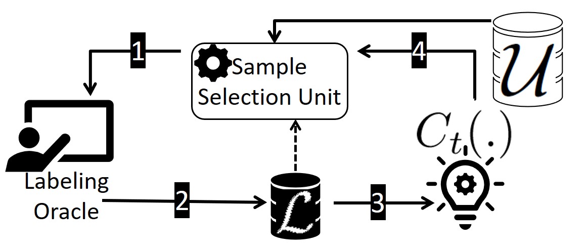
Figure 1. FAL framework.

At a high level, SSU can be viewed as two computation blocks stacked on top of each other. The upper block is the fairness-accuracy optimizer that selects a point from $\mathcal{U}$ to be labeled next such that a combination of accuracy (misclassification reduction) and fairness (unfairness reduction) is maximized. We shall provide the details of this block in § 5.

The accuracy-fairness optimizer relies on the lower block for estimating unfairness values. Let $C_{t-1}$ be the current model, created in the previous iteration $t-1$. In order to evaluate the unfairness reduction after labeling a sample point $\langle X^{(i)},S^{(i)}\rangle\in\mathcal{U}$, the optimizer block needs to compute the unfairness of the current model $\mathcal{F}(C_{t-1})$, as well as the unfairness of the model after labeling the sample point $\mathcal{F}(C_{t}^{i})$. Computing $\mathcal{F}(C_{t}^{i})$ turns out to be problematic as at the time of evaluating the candidate points in $\mathcal{U}$, we still do not know their labels. On the other hand, to evaluate $\mathcal{F}(C_{t}^{i})$, we need to know what the model parameters will be after labeling the point $\langle X^{(i)},S^{(i)}\rangle$ and adding it to $\mathcal{L}$. In other word, in order to evaluate a point to whether or not it should be labeled, we need to know its label in advance! This contradicts with the fact that $\mathcal{U}$ is unlabeled.

To resolve this issue, using a decision theoretic approach  (Settles, 2012), we consider the expected unfairness reduction: selecting the point that is expected to impart the largest reduction to the current model unfairness, after acquiring its label. Therefore, instead of $\mathcal{F}(C_{t})$ in Equation 3, we plug in the expected fairness $E\big{[}\mathcal{F}^{i}_{t}\big{]}$. In this way, we are approximating the expected future fairness of a model using $\mathcal{L}\cup X,\forall X\in\mathcal{U}$ over all possible labels under the current model. Consider a point $P_{i}\in\mathcal{U}$ and let $C^{i,k}_{t}$ be the model after adding $P_{i}$ to $\mathcal{L}$ if its true label is $y^{(i)}=k$. Inevitably, SSU does not know the label in advance. Hence, it must instead calculate the unfairness as an expectation over the possible labels. Equation 2 denotes the expected (un)fairness computation used by SSU:

(2) $$E\big{[}\mathcal{F}^{i}_{t}\big{]}=\sum_{k=0}^{K-1}\mathcal{F}(C^{i,K-1}_{t})\mathbb{P}(y=k|X^{(i)})$$

Using Figure 4 for explanation, for every point $P_{i}=\langle X^{(i)},S^{(i)}\rangle$ in the unlabeled pool, SSU considers different values of $\{0,\dots,K-1\}$ as possible labels for $P_{i}$. For every possible label $y_{k}$, it updates the model parameters to the intermediate model $C^{i,k}_{t}$ using $\mathcal{L}\cup\{\langle X^{(i)},S^{(i)},k\rangle\}$.

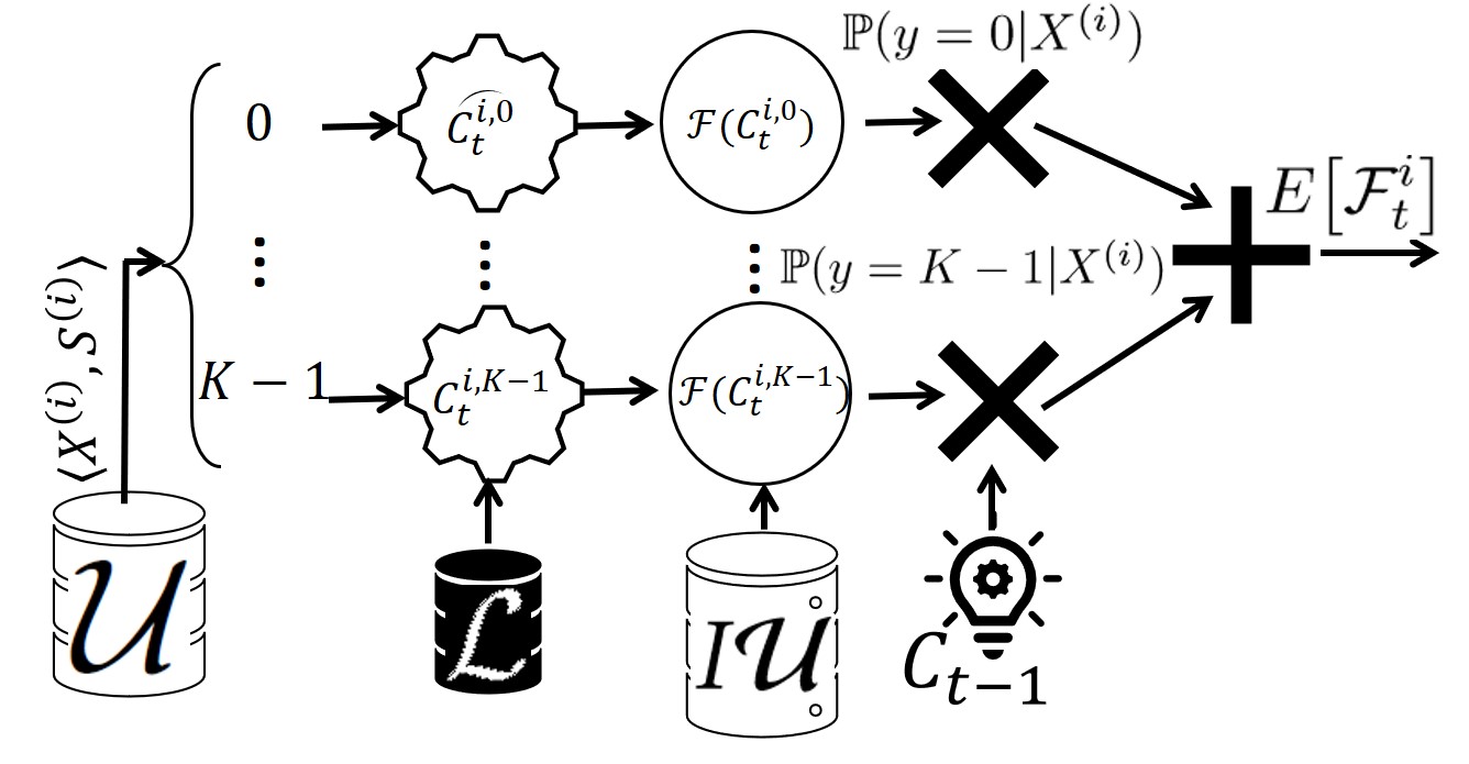
Figure 2. Computing expected unfairness for $\langle X^{(i)},S^{(i)}\rangle\in\mathcal{U}$.

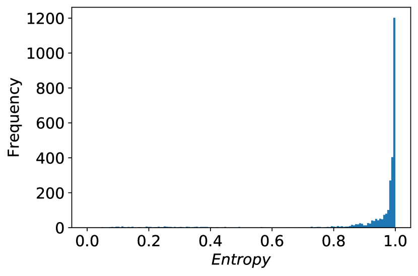
Figure 3. Distribution of entropy for COMPAS dataset.

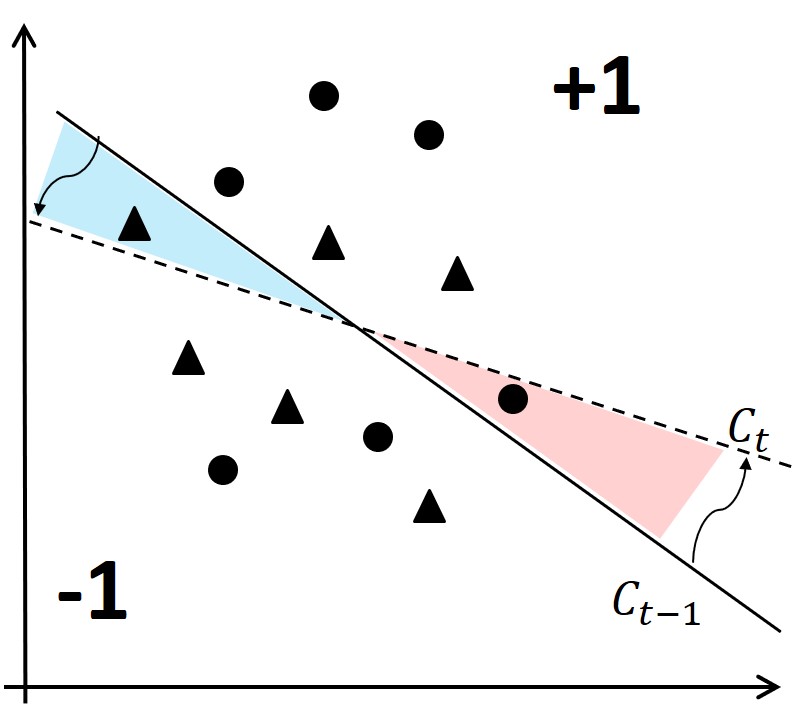
Figure 4. Toy example.

Algorithm 1 ExpF

0:  $\langle X^{(i)},S^{(i)}\rangle,\mathcal{L},C_{t-1}$

1:  $sum=0$

2:  for $k=0$ to $K-1$ do

3:     train $C^{i,k}_{t}$ using $\mathcal{L}\cup\{\langle X^{(i)},S^{(i)},y_{k}\rangle\}$

4:     compute $\mathcal{F}(C^{i,k}_{t})$, using $I\mathcal{U}$

5:     $sum=sum+\mathcal{F}(C^{i,k}_{t})\mathbb{P}(y=k|X^{(i)})$

6:  end for

7:  return $sum$

Since the points to be labeled are selective samples from $\mathcal{U}$, and moved from $\mathcal{U}$ to $\mathcal{L}$, after the process starts, neither $\mathcal{U}$ nor $\mathcal{L}$ can be seen as i.i.d. samples of the actual underlying distribution, and therefore, cannot be used to estimate the fairness. However, $\mathcal{U}$ initially follows the underlying distribution. Therefore, to create a dataset for evaluating the fairness of the model for sample selection, we utilize the initial unlabeled pool $\mathcal{U}$ (referred as $I\mathcal{U}$) and use it in different FAL iterations. Following the standard AL, at every iteration, for every possible label for a point $\langle X^{(i)},S^{(i)}\rangle$, SSU uses the current model $C_{t-1}$ for calculating $\mathbb{P}(y=k|X^{(i)})$. Algorithm 1 shows the pseudo-code of for computing the expected unfairness. In order to compute the expected unfairness, Algorithm 1 requires to train $K$ models, each for a possible label for the point $\langle X^{(i)},S^{(i)}\rangle$, which makes it inefficient. In § 6, we propose a constant-time approximation alternative that enables the same asymptotic time complexity as traditional active learning. We shall then provide the details of extending the fairness block for other measures of fairness beyond DP in § 7.

Having discussed the FAL framework and the unfairness estimation block, we will next describe the accuracy-fairness optimization block used by SSU for selecting the next sample to be labeled.

5. Accuracy-Fairness Optimization

5.1. FAL $\alpha$-aggregate

Similar to AL, FAL is also an iterative process that selects a sample from the unlabeled pool $\mathcal{U}$ to be labeled and added to the labeled pool $\mathcal{L}$. However, FAL $\alpha$-aggregate considers a combination of unfairness and misclassification error reduction as the optimization objective for the sampling step. Specifically, for a sample point $\langle X^{(i)},S^{(i)}\rangle\in\mathcal{U}$, we consider the Shannon entropy measure $\mathcal{H}_{t-1}(y^{(i)})$ for misclassification error, while considering demographic disparity $\mathcal{F}(C_{t}^{i})$ for unfairness — $C_{t}^{i}$ is the classifier trained on $\mathcal{L}$ at iteration $t$, after labeling the point $\langle X^{(i)},S^{(i)}\rangle$ and $\mathcal{H}_{t-1}(y^{(i)})$ is the entropy of the $y^{(i)}$ based on the current model $C_{t-1}$. The formulation can be viewed as a multi-objective optimization for fairness and misclassification error. Another perspective is to view the fairness as a regularization term to the optimization. Equation 3 is consistent with both of these views and is therefore considered in our framework.

(3) $$\operatorname*{argmax}_{\langle X^{(i)},S^{(i)}\rangle\in\mathcal{U}}\alpha\,\mathcal{H}_{t-1}(y^{(i)})+(1-\alpha)\big{(}\mathcal{F}(C_{t-1})-\mathcal{F}(C_{t}^{i})\big{)}$$

$(\mathcal{F}(C_{t-1})-\mathcal{F}(C_{t}^{i}))$ is the unfairness reduction (fairness improvement) term and the coefficient $\alpha\in[0,1]$ is the user-provided parameter that determines the trade-off between the model fairness and model performance. Values closer to $1$ put greater emphasize on model performance, while smaller values of $\alpha$ put greater importance on fairness. As we shall elaborate in § 8, entropy and fairness values are standardized to the same scale before being combined in Equation 3.

While $\alpha$ controls the trade-off between the accuracy (entropy) and the fairness terms, selecting an appropriate $\alpha$ value might not be clear for the user. More importantly, FAL might find it challenging to use a fixed learning strategy based on $\alpha$ in different iterations. To avoid parameter tuning in active learning instead of using a fixed $\alpha$ for all iterations, one can use a decay function that begins with a large value of $\alpha$, which improves the accuracy of the model. As the model becomes more stable, the value of $\alpha$ gets dropped, putting more weight on improving fairness. This concept is applied in different context, such as assigning learning rate (Schaul et al., 2013), where a larger value is used initially that gradually decreases over time. Our approach is agnostic to the decay function used. In the experiments, we use a function that linearly interpolates between the range [0,1]. The pseudo-code of FAL with $\alpha$-aggregate is provided in Algorithm 2.

Algorithm 2 FAL $\alpha$-aggregate

1:  for $t=1$ to $B$ do

2:     $max=0$

3:     for $i=1$ to $|\mathcal{U}|$ do

4:        H =$-\sum_{k=0}^{K-1}\mathbb{P}(y=k|X)\log\mathbb{P}(y=k|X)$

5:        $F=$ ExpF$\big{(}\langle X^{(i)},S^{(i)}\rangle,\mathcal{L},C_{t-1}\big{)}$

6:        $obj=\alpha(i)H+(1-\alpha(i))(\mathcal{F}(C_{t-1})-F)$

7:        if $obj>max$ then

8:           $max=obj$; $\langle X^{*},S^{*}\rangle=\langle X^{(i)},S^{(i)}\rangle$

9:        end if

10:     end for

11:     $y=$ label $X^{*}$ using the labeling oracle

12:     move $\langle X^{*},S^{*},y\rangle$ to $\mathcal{L}$

13:     train the classifier $C_{t}$ using $\mathcal{L}$

14:  end for

15:  return $C_{t}$

5.2. FAL Nested

Accurately estimating the expected unfairness reduction is critical for the performance of FAL. Looking at Equation 2, computing the expected fairness directly depends on the probability estimations of the current model $C_{t-1}$ for different class labels $k$. The miscalculation of these probabilities leads to an inaccurate estimation of fairness. Sacrificing accuracy for fairness in previous steps will affect the estimation of expected fairness in subsequent steps. Such erroneous estimation of the expected unfairness improvement as a result, contribute to the selection of points that do not support (and may even deteriorate) the fairness of the model and may not be good for model accuracy. In order to prevent this phenomena, it is necessary to always maintain an accurate intermediate model – i.e., to ensure that the selected points to be labeled will not negatively impact the accuracy of the model.

Fortunately, we make an observation in practice that helps us keeping the intermediate models accurate while achieving fairness. As we shall further explain in the following, our observation, also helps us to even reduce the computation cost of the model by only focusing on a subset of $\mathcal{U}$, instead of the full set.

It turns out in practice the distribution of the entropy of the data points in $\mathcal{U}$ is right-skewed, i.e. having a large number of points with entropy close to 1, i.e., all these points are almost equally good candidates from the accuracy perspective. We observed this in our real experiments, including the one on COMPAS dataset shown in Figure 4.

Consider the set of points on the right-most bucket with entropy close to one. Any of the points in this set are good candidates from lens of active learning (Equation 1) to ensure the high quality of the intermediate models. On the other hand, the relatively large size of the set (as observed in Figure 4) increases the chance that it contains a point with a high potential for reducing unfairness.

We use the above observation to design a nested optimization for accuracy and fairness. In particular, instead of computing a score by linearly combining the two terms (Equation 3), we apply a nested optimization where in the first level, we select a subset of $\mathcal{U}_{A}\subset\mathcal{U}$ of the top-$\ell$ points that maximize the entropy $\mathcal{H}(y^{(i)})$ using the current classifier $C_{t-1}$:

(4) $$\mathcal{U}_{A}=\underset{\langle X^{(i)},S^{(i)}\rangle\in\mathcal{U}}{\ell\mbox{-argmax}}\mathcal{H}(y|X,\mathcal{L})$$

where the function $\ell$-argmax returns $\ell$ samples with maximum values. The first optimization level only optimizes for accuracy, to ensure maintaining a high accuracy for the intermediate model. Next, changing the optimization criteria to fairness in the second level, SSU selects a point from $\mathcal{U}_{A}$ that maximizes the unfairness improvement (Equation 5) and pass it to the labeling oracle.

$$\operatorname*{argmax}_{\langle X^{(i)},S^{(i)}\rangle\in\mathcal{U}_{A}}\big{(}\mathcal{F}(C_{t-1})-\mathcal{F}(C_{t}^{i})\big{)}$$

(5) $$= \operatorname*{argmin}_{\langle X^{(i)},S^{(i)}\rangle\in\mathcal{U}_{A}}\mathcal{F}(C_{t}^{i})$$

Besides assuring the accurate estimations of expected unfairness reduction, the nested optimization helps to reduce the time-complexity of FAL. This is especially important as it reduces the number of points to be evaluated for fairness from $|\mathcal{U}|$ to $\ell$. Note that, in order to estimate the unfairness reduction for every sample (Figure 4), Algorithm 1 requires retraining of $k$ models. As a result, the computation time to run the framework is dominated by the total time to compute fairness values for the points in the unlabeled pool, before selecting one to be labeled. Hence, reducing the number of points to be evaluated for fairness significantly reduces the computation cost by a factor of $\frac{\ell}{|\mathcal{U}|}$.

5.3. FAL Nested-Append

Since the sample points in $\mathcal{U}$ are unlabeled, FAL has no choice but to estimate the expected unfairness reduction after labeling a point, according to how likely it will take each possible label. But whether unfairness reduces depends on the actual label after adding the point to $\mathcal{L}$. To further clarify this, let us consider a toy example highlighted in Figure 4. To simplify the explanation, we use 6 triangle and 6 circle points, each representing a demographic group, to evaluate the fairness of a linear binary classifier. Suppose the decision boundary of current classifier ($C_{t-1}$) is the one shown in solid line in the figure, and the points in the top-right of the line are classified as +1. $C_{t-1}$ classifies two third (4 out of 6) of circles, but only one third (2 out of 6) of triangles as +1, hence is not fair according to DP.

Looking at the figure, to make the classifier fair, FAL needs to rotate the border towards the dashed line. Consider the two angles highlighted in the figure in the intersection of the two lines. To make the rotation, FAL needs to find points in $\mathcal{U}$ with the true +1 label that belong to the top-left angle, or the ones with the true -1 label in the bottom-right angle. Note that such points are misclassified by the current classifier. As a result, it is less likely to find the points with proper labels needed for reducing unfairness. On the other hand, if the label is not as hoped, adding the new point will not help to reduce unfairness. Therefore, to boost FAL for improving fairness, our next optimization, FAL Nested-Append, replicates the points that get labeled in a way that unfairness gets reduced. Let $\tilde{P}_{i}=\langle\tilde{X}^{(i)},\tilde{S}^{(i)}\rangle\in\mathcal{U}_{A}$ be the point selected using FAL Nested. Let $\mathcal{F}(C_{t})$ be the unfairness of the model after collecting the true label of $\tilde{P}_{i}$ and adding it to $\mathcal{L}$. If $\mathcal{F}(C_{t})-\mathcal{F}(C_{t-1})>0$, the algorithm replicates $\tilde{P}_{i}$ in $\mathcal{L}$, further boosting its impact for unfairness reduction. In particular, since FAL Nested puts more emphasize on accuracy, FAL Nested-Append helps to account more for fairness. As we shall show in § 8, boosting the performance of FAL Nested for fairness, FAL Nested-Append had the best performance across different experiments.

6. Efficient FAL by Covariance

Our proposed FAL framework is agnostic to the choice of classifier $C$. In this section, we show that it is possible to design efficient algorithm for the special case of generalized linear models. An appealing property of our algorithm is that, using the efficient computation provided in Appendix A, it has same asymptotic time complexity as traditional active learning. We achieve this by avoiding the model retraining step for calculating the expected fairness of unlabeled samples, in Algorithm 1.

Consider a generalized linear model in form of $\hat{y}=\theta^{\top}X$. The covariance between the model and a sensitive attribute $S$ should be zero under model independence (demographic parity). We make a key observation in Lemma 1 that shows this covariance, $cov(S,\hat{y})$, only depends on $cov(S,X)$ and $\theta$.

Lemma 1.

For a generalized linear model in form of $\hat{y}=\theta^{\top}X$, $cov(S,\hat{y})=\theta^{\top}cov(S,X)$.

According to Lemma 1, the covariance of the model with the sensitive attribute (that results in unfairness) depends only on the weight vector $\theta$ and the underlying covariance of features $X$ with $S$. We can reduce the model unfairness by ensuring that the model does not assign high weights to the problematic features (the features with high covariance with $S$). This observation allows us to indirectly optimize for fairness through covariance instead of computing expected unfairness reduction.

Consider a feature $x_{i}$ that is highly correlated with the sensitive attribute (i.e., $cov(x_{i},S)$ is high) and also has a high weight $\theta_{i}$ in the current model. Our objective is to reduce the weight assigned to such features. The reason the model has assigned a large weight to $x_{i}$ is that $x_{i}$ is highly predictive of $y$ in $\mathcal{L}$. Therefore, in order to reduce the weight $\theta_{i}$, we need to reduce $cov_{\mathcal{L}}(x_{i},y)$ in the labeled pool $\mathcal{L}$ to make it less predictive of $y$ in $\mathcal{L}$. Now, consider a point $P_{j}=\langle X^{(j)},S^{(j)}\rangle\in\mathcal{U}$ and its value $X^{(j)}_{i}$ on feature $x_{i}$. Depending on $X^{(j)}_{i}$ and its label $y^{(j)}$ (after labeling), the point $P_{j}$ can impact $cov(x_{i},y)$ in $\mathcal{L}$. Indeed, we don’t know $y^{(j)}$ during the sample selection step. Still, similar to § 5, we can consider the probability distribution over $y$ and calculate the expected improvement in covariance. Let $cov_{i}=cov_{\mathcal{L}}(x_{i},y)$ be the covariance of $x_{i}$ and $y$ in $\mathcal{L}$ and $cov_{j,i,k}=cov_{\mathcal{L}\cup\{\langle X^{(j)},S^{(j)},k\rangle\}}(x_{i},y)$ the covariance of $x_{i}$ and $y$ after adding $\langle X^{(j)},S^{(j)},k\rangle$ to $\mathcal{L}$. The expected covariance improvement for $x_{i}$ after adding $P_{j}$ to $\mathcal{L}$ is

(6) $$E\big{[}cov^{\downarrow}_{j,i}\big{]}=\sum_{k=0}^{K-1}(|cov_{i}|-|cov_{j,i,k}|)\mathbb{P}(y=k|X^{(j)})$$

Following Lemma 1 the contribution of the covariance reduction for a feature $x_{i}$ to fairness is proportional to $|\theta_{i}cov(x_{i},S)|$. Subsequently, it is important to reduce $cov_{\mathcal{L}}(x_{i},y)$ for the features that are highly correlated with the sensitive attribute and have a high weight $\theta_{i}$ in the model. Therefore, the (indirect) fairness improvement by covariance for a point $P_{j}\in\mathcal{U}$ can be computed as following:

(7) $$E\big{[}FbC^{\downarrow}_{j}\big{]}=\sum\limits_{i=1}^{d}|\theta_{i}cov(S,x_{i})|E\big{[}cov^{\downarrow}_{j,i}\big{]}$$

Now, it is enough to replace the term for expected unfairness reduction $\big{(}\mathcal{F}(C_{t-1})-\mathcal{F}(C_{t}^{i})\big{)}$, in Equations 3 and 5, with $E\big{[}FbC^{\downarrow}_{i}\big{]}$.

7. Extension to Other Fairness Models

So far in this paper, we considered independence ($\hat{y}\bot S$) for fairness. Next, we discuss how to extended our findings to other measures based on separation and sufficiency (Barocas et al., 2019), such as equalized odds (Hardt et al., 2016), where the prediction outcome $\hat{y}$ is independent of the sensitive feature $S$ given the true label $y$, i.e. $P(\hat{y}=1|y=1,S=0)=P(\hat{y}=1|y=1,S=1),y\in{0,1}$.

The fairness-accuracy optimizer of FAL is not limited to a specific notion of fairness for balancing accuracy and fairness. Similarly, the notion of expected unfairness reduction does not rely on a specific notion of fairness as $\mathcal{F}(.)$ in Equation 2 can be computed using any fairness measure, besides demographic parity. As a result, at a high-level, the FAL framework should work as-is for other notions of fairness as well. However, as we shall explain in the following, computing $\mathcal{F}(.)$ would require additional information that comes at a cost of randomly labeling a subset of data.

Looking at Figure 4, recall that we use the initial unlabeled set $I\mathcal{U}$ for estimating the fairness of a model. $I\mathcal{U}$ follows the underlying data distribution and, hence, can be used for evaluating the demographic disparity. However, this set cannot be used for estimating fairness according to separation or sufficiency since its instances are not labeled. On the other hand, the pool of labeled data are not representative of the underlying data distribution.

Our resolution is to use a small subset of $\mathcal{C}_{\mathcal{U}}\subset I\mathcal{U}$ for fairness computation, accepting the potential error in estimations relative to the size of the set. Before starting the FAL process, we need to label $\mathcal{C}_{\mathcal{U}}$. Once labeled, $\mathcal{C}_{\mathcal{U}}$ will be used for calculating $\mathcal{F}(.)$ based on other notions of fairness, and FAL can be executed as-is. In § 8, we run experiments to show the extension of FAL for equalized odds.

8. Experiments

The experiments were performed on a Linux machine with a Core I9 CPU and 128GB memory. The algorithms were implemented using Python 3.7 .

8.1. Datasets

COMPAS: published by ProPublica (Angwin et al., 2016), this dataset contains information of juvenile felonies such as marriage status, race, age, prior convictions, and the charge degree of the current arrest. We normalized data so that it has zero mean and unit variance. We consider race as sensitive attribute and filtered dataset to black and white defendants. The dataset contains 5,875 records, after filtering. Following the standard practice (Corbett-Davies et al., 2017; Mehrabi et al., 2019), we use two-year violent recidivism record as the true label of recidivism: $y^{(i)}=1$ if the recidivism is greater than zero and $y^{(i)}=0$ otherwise.

Adult dataset: contains 45,222 individuals income extracted from the 1994 census data with attributes such as age, occupation, education, race, sex, marital-status, hours-per-week, native country, etc. We use income (a binary attribute with values $\geq 50k$$ and $\leq 50k$$) as the true label. We consider sex as the sensitive attribute. We normalized data so that it has zero mean and unit variance.

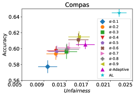
(a) FAL $\alpha$-aggregate

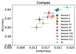
(b) FAL Nested

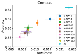
(c) FAL Nested-Append

(d) FAL $\alpha$-aggregate

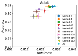
(e) FAL Nested

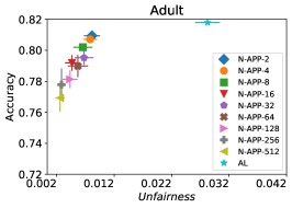
(f) FAL Nested-Append

Figure 5. The average DP and accuracy of different FAL approaches.

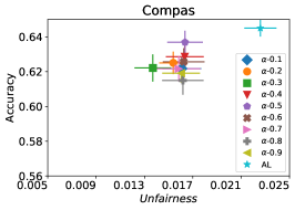
(a) FBC $\alpha$-aggregate

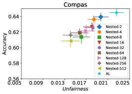
(b) FBC Nested

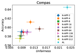
(c) FBC Nested-Append

Figure 6. The average DP and accuracy of different FBC approaches, COMPAS Dataset.

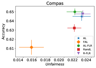
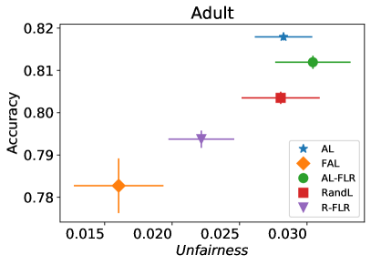
Figure 7. Comparison with baselines.

Figure 8. FAL with Equalized odds, COMPAS Dataset.

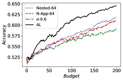
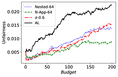
Figure 9. Performance evaluation over budget.

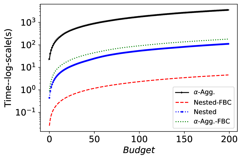
Figure 10. Computation time.

8.2. Algorithms Evaluated

All our proposed approaches are evaluated using a regularized $\ell_{2}$ norm logistic regression classifier with a regularization strength of one. We trained the logistic regression with liblinear optimizer and with maximum iteration of 100. Our findings are transferable to other classifiers. We begin by comparing our proposed approach against a wide variety of representative baselines. Then, we focus on understanding the effectiveness and performances of our proposed approaches under different settings.

Baselines: We consider four baselines in order to build a fair classifier in a limited data environment. We first start to evaluate passive methods, RandL and R-FLR, that select all the samples randomly at one shot to form a training set and fit a regular and fair logistic regression (proposed by  (Zafar et al., 2017)), respectively. We then evaluate active methods, AL and AL-FLR, which iteratively select a sample point based on its informativeness (Equation 1) and fits a regular and fair logistic regression  (Zafar et al., 2017) in each iteration, respectively.

Our Algorithms: We evaluate our fairness-accuracy optimization algorithms proposed in § 5, namely FAL $\alpha$-aggregate (FAL-$\alpha$), FAL Nested (Nested), and FAL Nested-Append (N-App). For FAL-$\alpha$, we normalize the accuracy and fairness improvement values as ($v$-min)/(max-min) before combining them in Equation 3. Besides fixed values of $\alpha$, we also consider an adaptive $\alpha$ parameter, using a decay function that, starting from $\alpha=1$ to $\alpha=0$, the value $\alpha$ drops by 0.1 every $\lfloor B/11\rfloor$ iterations. For Nested, and N-App, we consider different exponents of 2 as the value of $\ell$ (in Equation 4) from $2$ to $512$.

Our default choice for computing unfairness reduction is Algorithm 1. The efficient FAL by covariance (FBC), proposed in §6, is also evaluated to show the computation time improvement. We evaluate FBC with the three optimization approaches FAL-$\alpha$, Nested, and N-App. Finally, in order to show the extension of our proposal for other fairness models, we run FAL using Equalized Odds as the fairness measure.

8.3. Performance Evaluation

We perform the experiments using 30 random splits of the datasets into training $\mathcal{U}$ ($60\%$ of the examples) and testing ($40\%$ of the examples). We consider the mean and variance over the 30 random splits. We specify the maximum labeling budget to 200 after which performance leveled off. In each FAL and AL scenarios, we start with six labeled points and sequentially select points to label, until the budget is exhausted. Mutual information is our default measure of demographic parity.

We first evaluate the performance of FAL-$\alpha$ versus the passive and active baselines RandL, R-FLR, AL, and AL-FLR, using accuracy and fairness measures to show the deficiency of these approaches in construction of a final fair classifier. Figure 8 illustrates the performance of baselines and FAL-$\alpha$ where $\alpha=0.6$ for COMPAS and Adult datasets. The bars indicate the standard deviation on 30 random split of data. We observe that the baselines had similar performances on fairness. Even applying a fair classifier (FLR) fails to improve the fairness. FAL-$\alpha$, on the other hand, significantly reduces unfairness while sustaining a comparable accuracy.

In our next experiment illustrated in Figure 5, we evaluate the average performance of three different optimizers FAL-$\alpha$, Nested, and N-App, the efficient algorithms proposed in §5 and compare it against AL. Figure 5(a) presents a comprehensive comparison of FAL with different user-defined $\alpha$ and adaptive alpha, versus AL on COMPAS dataset. We can observe that FAL-$\alpha$ achieved a good level of fairness across different $\alpha$ values. Figure 5(b) corresponds to the performance of Nested, which focuses on the upper percentile of the entropy distribution, to ensure that the selected points are improving accuracy, and not only the unfairness. As expected, the results indicate that this approach nudges up the accuracy of FAL-$\alpha$. Finally, in Figure 5(c), we evaluate the average performance of N-App on COMPAS dataset. Compared to both FAL-$\alpha$ and Nested, the unfairness level of the model dramatically improved by appending the points two times when they truly improve the unfairness level in each iteration. Similarly, we replicated the results for Adult dataset as in Figure 5(d), 5(e), and 5(f). It can be seen that the effective N-App approach significantly improves the unfairness level of the model while maintaining its accuracy.

We also evaluate the average performance of FBC approach as proposed in §6. Figure 6 includes the results of FBC with the three proposed optimizers on COMPAS dataset (the results for Adult dataset are provided in Appendix C). The results are fairly consistent with the results we observed in Figure 5 for COMPAS dataset. Note that FBC is an approximation of the expected unfairness reduction and is computationally more efficient to be used in FAL algorithm (Figure 10). As we discussed in §7, our proposed approaches can be extended to use other fairness measures. Figure 8 corresponds to the experimental setup where he Equalized Odds notion of fairness as proposed in (Hardt et al., 2016) is used in FAL-$\alpha$ for measuring fairness. The results indicate the effectiveness of FAL compared to AL using different $\alpha$ values. The results of the same setting for Adult dataset is provided in Figure 13(a) in Appendix.

Figure 10 corresponds to the average (un)fairness and average accuracy score on 30 random runs. Looking at the figure, we can observe that Nested-64 enforces the accuracy while considering the fairness in the sample selection. Hence, with a higher accuracy and lower unfairness it outperforms FAL-$\alpha$-0.6. Note that the performance of N-App-64, outperforms both FAL-$\alpha$-0.6 and Nested-64 as expected.

Figure 10 shows the computation time of each sampling iteration for different accuracy-fairness optimizers compared to the original FAL. FBC is orders of magnitude faster than FAL as it avoids the need to compute expected fairness. On the other hand, since it indirectly optimizes for fairness, FAL outperforms it on fairness.

9. Final Remarks

Prior works on fair classification assume the availability of sufficiently labeled data. In a number of societal applications such as recidivism prediction, the labeled data is unavailable and collecting it is expensive and time-consuming. The traditional active learning approach focuses on accuracy, often at the cost of fairness. In this paper, we proposed a framework for fairness in active learning that balances fairness and accuracy by selecting samples from the unlabeled pool that maximizes a linear combination of misclassification error reduction and improvement over expected fairness. We described a wide variety of optimizations for improving accuracy, fairness, and running time. Specifically, FAL Nested-Append successfully achieves a deft balance between accuracy and fairness. Our extensive experiments on real datasets confirm that our proposed approach produces a fairer model without significantly sacrificing the accuracy. We hope that our proposed approach will have a positive impact by improving 1the model fairness in a number of real-world scenarios.

Appendix

Appendix A Efficiently Computing Covariance of $X$ and $y$ in $\mathcal{L}$

When the number of features $d$ is a constant, it is possible to further improve the efficiency by computing $E\big{[}FbC^{\downarrow}_{j}\big{]}$ in constant time by maintaining the aggregates from the previous steps. Therefore, the time complexity of the fair active learning framework (without considering the labeling cost) drops from $O(B\cdot T\cdot|\mathcal{U}|)$ to $O\big{(}B\cdot(|\mathcal{U}|+T)\big{)}$, the same as traditional active learning.

First, we note that $cov(x_{i},S)$, the covariance of each feature $x_{i}$ with $S$, does not depend on $\mathcal{L}$ and can be computed in advance, using the unlabeled samples in $\mathcal{U}$. It is computed once for every feature at the beginning of the process and the same numbers will be used in different iterations. The values of $cov_{i}=cov_{\mathcal{L}}(x_{i},y)$ and $cov_{j,i,k}=cov_{\mathcal{L}\cup\{\langle X^{(j)},S^{(j)},y^{(j)}=k\rangle\}}(x_{i},y)$ in Equation 6, however, depend on the set of labeled data and should get recomputed at different iterations and for different points $P_{j}\in\mathcal{U}$. We maintain the following aggregates for efficiently computing these values:

$$~{}\mathcal{G}_{y}~{}=\sum_{\forall\langle X^{(\ell)},S^{(\ell)},y^{(\ell)}\rangle\in\mathcal{L}}y^{(\ell)}$$

$$\forall i\in[1,d]:~{} \mathcal{G}_{x}[i]=\sum_{\forall\langle X^{(\ell)},S^{(\ell)},y^{(\ell)}\rangle\in\mathcal{L}}X^{(\ell)}_{i}$$

$$\forall i\in[1,d]:~{} \mathcal{G}_{z}[i]=\sum_{\forall\langle X^{(\ell)},S^{(\ell)},y^{(\ell)}\rangle\in\mathcal{L}}X^{(\ell)}_{i}y^{(\ell)}$$

Note that at every iteration each of the above aggregates can be updated in constant time by adding the corresponding value from the new point to it. Now, using these aggregates:

$$cov_{i}=cov_{\mathcal{L}}(x_{i},y)=\frac{\mathcal{G}_{z}[i]}{n}-\frac{\mathcal{G}_{x}[i]}{n}\times\frac{\mathcal{G}_{y}}{n}$$

Similarly, for a point $P_{j}=\langle X^{(j)},S^{(j)}\rangle\in\mathcal{U}$ and a label $y^{(j)}=k$:

$$cov_{j,i,k}=\frac{\mathcal{G}_{z}[i]+kX^{(j)}_{i}}{n+1}-\frac{\mathcal{G}_{x}[i]+X^{(j)}_{i}}{n+1}\times\frac{\mathcal{G}_{y}+k}{n+1}$$

Appendix B Proof of Lemma 1

$$cov(S,\hat{y}) =E[S\,\hat{y}]-E[S]E[\hat{y}]$$

$$E[S]E[\hat{y}] =\mu_{S}E\big{[}\sum\theta_{i}x_{i}\big{]}=\mu_{S}\sum\theta_{i}\mu_{x_{i}}$$

$$=\theta_{1}\mu_{S}\mu_{x_{1}}+\theta_{2}\mu_{S}\mu_{x_{2}}+\cdots+\theta_{d}\mu_{S}\mu_{x_{d}}$$

$$E[S\hat{y}] =E\big{[}S\,\sum\theta_{i}x_{i}\big{]}=E\big{[}\sum S\,\theta_{i}x_{i}\big{]}$$

$$=E\big{[}S\,\theta_{1}x_{1}+S\,\theta_{2}x_{2}+\cdots+S\,\theta_{d}x_{d}\big{]}$$

$$=E\big{[}S\,\theta_{1}x_{1}\big{]}+E\big{[}S\,\theta_{2}x_{2}\big{]}+\cdots+E\big{[}S\,\theta_{d}x_{d}\big{]}$$

$$=\theta_{1}E\big{[}S\,x_{1}\big{]}+\cdots+\theta_{d}E\big{[}S\,x_{d}\big{]}$$

$$\Rightarrow cov(S,\hat{y}) =\theta_{1}E\big{[}S\,x_{1}\big{]}+\cdots+\theta_{d}E\big{[}S\,x_{d}\big{]}-$$

$$~{}~{}~{}~{}(\theta_{1}\mu_{S}\mu_{x_{1}}+\cdots+\theta_{d}\mu_{S}\mu_{x_{d}})$$

$$=\theta_{1}(E\big{[}S\,x_{1}\big{]}-\mu_{S}\mu_{x_{1}})+\cdots+\theta_{d}(E\big{[}S\,x_{d}\big{]}-\mu_{S}\mu_{x_{d}})$$

$$=\sum\limits_{i=1}^{d}\theta_{i}cov(S,x_{i})=\theta^{\top}cov(S,X)$$

Appendix C Complimentary Experiment Results

In this section, we provide additional experimental results on the performance of our proposed algorithms, using FBC and Equalized Odds.

Figure 11 presents results for FBC approach using three different optimizers, FAL-$\alpha$, Nested, and N-App on Adult dataset. It can be seen that our ideal N-App approach outperforms other optimizers when we use the efficient FBC approach for fairness approximation.

In Figure 8 we provided our experiment results for Equalized Odds, using N-App, on COMPAS dataset. Figure 12 shows our complimentary results for the other two accuracy-fairness optimizers: FAL-$\alpha$ and Nested.

Finally, Figure 13 provides results of FAL using three different optimizer for Equalized Odds on Adult dataset. The results indicate that our efficient and effective N-App approach outperforms other optimizers in terms of unfairness reduction while maintaining accuracy.

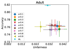
(a) FBC $\alpha$-aggregate

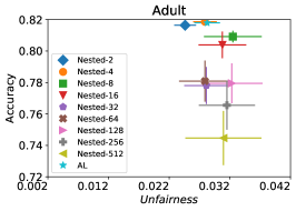
(b) FBC Nested

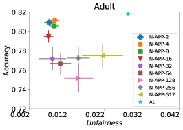
(c) FBC Nested-Append

Figure 11. The average DP and accuracy of different FBC approaches, Adult Dataset.

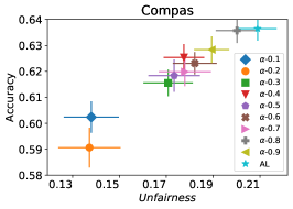
(a) $\alpha$-aggregate

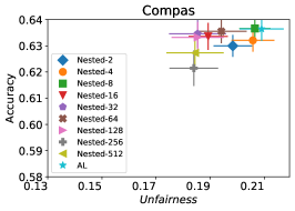
(b) Nested

Figure 12. Equalized Odds, COMPAS Dataset.

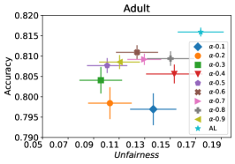
(a) $\alpha$-aggregate

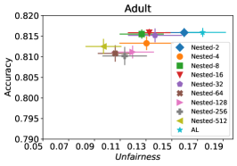
(b) Nested

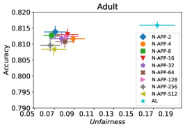
(c) Nested-Append

Figure 13. Equalized Odds, Adult Dataset.

References

- (1)
- Angwin et al. (2016) J. Angwin, J. Larson, S. Mattu, and L. Kirchner. 2016. Machine Bias: Risk Assessments in Criminal Sentencing. ProPublica (2016). https://bit.ly/2s0UMfA
- Asudeh et al. (2019) Abolfazl Asudeh, Zhongjun Jin, and HV Jagadish. 2019. Assessing and remedying coverage for a given dataset. In ICDE. IEEE, 554–565.
- Bakker et al. (2020) M. A Bakker, H. R. Valdés, D. P. Tu, K. P Gummadi, K. R Varshney, A. Weller, and A. Pentland. 2020. Fair Enough: Improving Fairness in Budget-Constrained Decision Making Using Confidence Thresholds.. In SafeAI@ AAAI.
- Balcan et al. (2007) Maria-Florina Balcan, Andrei Broder, and Tong Zhang. 2007. Margin based active learning. In COLT. Springer, 35–50.
- Barocas et al. (2017) Solon Barocas, Moritz Hardt, and Arvind Narayanan. 2017. Fairness in machine learning. NIPS Tutorial (2017).
- Barocas et al. (2019) Solon Barocas, Moritz Hardt, and Arvind Narayanan. 2019. Fairness and machine learning: Limitations and opportunities. fairmlbook.org.
- Barocas and Selbst (2016) Solon Barocas and Andrew D Selbst. 2016. Big data’s disparate impact. Calif. L. Rev. 104 (2016), 671.
- Beutel et al. (2019) Alex Beutel, Jilin Chen, Tulsee Doshi, Hai Qian, Li Wei, Yi Wu, Lukasz Heldt, Zhe Zhao, Lichan Hong, Ed H Chi, et al. 2019. Fairness in recommendation ranking through pairwise comparisons. In SIGKDD. 2212–2220.
- Buolamwini and Gebru (2018) Joy Buolamwini and Timnit Gebru. 2018. Gender shades: Intersectional accuracy disparities in commercial gender classification. In FAccT. 77–91.
- Celis et al. (2019) L Elisa Celis, Lingxiao Huang, Vijay Keswani, and Nisheeth K Vishnoi. 2019. Classification with fairness constraints: A meta-algorithm with provable guarantees. In FAccT. ACM, 319–328.
- Corbett-Davies et al. (2017) Sam Corbett-Davies, Emma Pierson, Avi Feller, Sharad Goel, and Aziz Huq. 2017. Algorithmic decision making and the cost of fairness. In SIGKDD. ACM, 797–806.
- DiCiccio et al. (2020) Cyrus DiCiccio, Sriram Vasudevan, Kinjal Basu, Krishnaram Kenthapadi, and Deepak Agarwal. 2020. Evaluating fairness using permutation tests. In SIGKDD.
- Donmez et al. (2007) Pinar Donmez, Jaime G Carbonell, and Paul N Bennett. 2007. Dual strategy active learning. In ECIR.
- Dwork et al. (2012) Cynthia Dwork, Moritz Hardt, Toniann Pitassi, Omer Reingold, and Richard Zemel. 2012. Fairness through awareness. In ITCS. ACM, 214–226.
- Feldman et al. (2015) Michael Feldman, Sorelle A Friedler, John Moeller, Carlos Scheidegger, and Suresh Venkatasubramanian. 2015. Certifying and removing disparate impact. In SIGKDD.
- Fish et al. (2016) Benjamin Fish, Jeremy Kun, and Ádám D Lelkes. 2016. A confidence-based approach for balancing fairness and accuracy. In SDM. SIAM, 144–152.
- Geyik et al. (2019) Sahin Cem Geyik, Stuart Ambler, and Krishnaram Kenthapadi. 2019. Fairness-aware ranking in search & recommendation systems with application to linkedin talent search. In SIGKDD. 2221–2231.
- Goh et al. (2016) Gabriel Goh, Andrew Cotter, Maya Gupta, and Michael P Friedlander. 2016. Satisfying real-world goals with dataset constraints. In NeurIPS. 2415–2423.
- Hardt et al. (2016) Moritz Hardt, Eric Price, Nati Srebro, et al. 2016. Equality of opportunity in supervised learning. In NeurIPS. 3315–3323.
- Hébert-Johnson et al. (2017) Ursula Hébert-Johnson, Michael P Kim, Omer Reingold, and Guy N Rothblum. 2017. Calibration for the (computationally-identifiable) masses. arXiv preprint arXiv:1711.08513 (2017).
- Huang and Vishnoi (2019) Lingxiao Huang and Nisheeth K Vishnoi. 2019. Stable and Fair Classification. arXiv preprint arXiv:1902.07823 (2019).
- Huang et al. (2010) Sheng-Jun Huang, Rong Jin, and Zhi-Hua Zhou. 2010. Active learning by querying informative and representative examples. In NeurIPS. 892–900.
- Jan (2018) Tracy Jan. 2018. Redlining was banned 50 years ago. It’s still hurting minorities today. Washington Post.
- Jones (1983) Frank L Jones. 1983. Sources of gender inequality in income: what the Australian Census says. Social Forces 62, 1 (1983), 134–152.
- Kamiran and Calders (2012) Faisal Kamiran and Toon Calders. 2012. Data preprocessing techniques for classification without discrimination. KAIS 33, 1 (2012), 1–33.
- Kim et al. (2018) Michael P Kim, Amirata Ghorbani, and James Zou. 2018. Multiaccuracy: Black-box post-processing for fairness in classification. arXiv preprint arXiv:1805.12317 (2018).
- Komiyama et al. (2018) Junpei Komiyama, Akiko Takeda, Junya Honda, and Hajime Shimao. 2018. Nonconvex optimization for regression with fairness constraints. In ICML.
- Krasanakis et al. (2018) Emmanouil Krasanakis, Eleftherios Spyromitros-Xioufis, Symeon Papadopoulos, and Yiannis Kompatsiaris. 2018. Adaptive sensitive reweighting to mitigate bias in fairness-aware classification. In WWW. 853–862.
- Kusner et al. (2017) Matt J Kusner, Joshua Loftus, Chris Russell, and Ricardo Silva. 2017. Counterfactual fairness. In NeurIPS. 4066–4076.
- Lewis and Catlett (1994) David D Lewis and Jason Catlett. 1994. Heterogeneous uncertainty sampling for supervised learning. In Machine learning proceedings 1994. Elsevier, 148–156.
- Lewis and Gale (1994) David D Lewis and William A Gale. 1994. A sequential algorithm for training text classifiers. In SIGIR’94. Springer, 3–12.
- Li et al. (2020) Yanying Li, Haipei Sun, and Wendy Hui Wang. 2020. Towards Fair Truth Discovery from Biased Crowdsourced Answers. In SIGKDD. 599–607.
- Mehrabi et al. (2019) Ninareh Mehrabi, Fred Morstatter, Nripsuta Saxena, Kristina Lerman, and Aram Galstyan. 2019. A survey on bias and fairness in machine learning. arXiv preprint arXiv:1908.09635 (2019).
- Menon and Williamson (2018) Aditya Krishna Menon and Robert C Williamson. 2018. The cost of fairness in binary classification. In FAccT. 107–118.
- Noriega-Campero et al. (2019) Alejandro Noriega-Campero, Michiel A Bakker, Bernardo Garcia-Bulle, and Alex’Sandy’ Pentland. 2019. Active fairness in algorithmic decision making. In AIES. 77–83.
- Pleiss et al. (2017) Geoff Pleiss, Manish Raghavan, Felix Wu, Jon Kleinberg, and Kilian Q Weinberger. 2017. On fairness and calibration. In NeurIPS. 5680–5689.
- Schaul et al. (2013) Tom Schaul, Sixin Zhang, and Yann LeCun. 2013. No more pesky learning rates. In ICML. 343–351.
- Settles (2012) Burr Settles. 2012. Active Learning. In Synthesis Lectures on Artificial Intelligence and Machine Learning 18. 1–111.
- Shannon (1948) Claude Elwood Shannon. 1948. A mathematical theory of communication. Bell system technical journal 27, 3 (1948), 379–423.
- Sharaf and Daumé III ([n.d.]) Amr Sharaf and Hal Daumé III. [n.d.]. Promoting Fairness in Learned Models by Learning to Active Learn under Parity Constraints. ([n. d.]).
- Simoiu et al. (2017) Camelia Simoiu, Sam Corbett-Davies, Sharad Goel, et al. 2017. The problem of infra-marginality in outcome tests for discrimination. The Annals of Applied Statistics 11, 3 (2017), 1193–1216.
- Speicher et al. (2018) Till Speicher, Hoda Heidari, Nina Grgic-Hlaca, Krishna P Gummadi, Adish Singla, Adrian Weller, and Muhammad Bilal Zafar. 2018. A unified approach to quantifying algorithmic unfairness: Measuring individual &group unfairness via inequality indices. In SIGKDD. 2239–2248.
- Srivastava et al. (2019) Megha Srivastava, Hoda Heidari, and Andreas Krause. 2019. Mathematical notions vs. human perception of fairness: A descriptive approach to fairness for machine learning. In SIGKDD. 2459–2468.
- Tong and Koller (2001) Simon Tong and Daphne Koller. 2001. Support vector machine active learning with applications to text classification. JMLR 2, Nov (2001), 45–66.
- Xu et al. (2003) Zhao Xu, Kai Yu, Volker Tresp, Xiaowei Xu, and Jizhi Wang. 2003. Representative sampling for text classification using support vector machines. In European conference on information retrieval. Springer, 393–407.
- Zafar et al. (2017) Muhammad Bilal Zafar, Isabel Valera, Manuel Gomez Rodriguez, and Krishna P Gummadi. 2017. Fairness beyond disparate treatment & disparate impact: Learning classification without disparate mistreatment. In WWW. 1171–1180.
- Zemel et al. (2013) Rich Zemel, Yu Wu, Kevin Swersky, Toni Pitassi, and Cynthia Dwork. 2013. Learning fair representations. In ICML. 325–333.
- Žliobaitė (2017) Indrė Žliobaitė. 2017. Measuring discrimination in algorithmic decision making. Data Mining and Knowledge Discovery 31, 4 (2017), 1060–1089.
- Zou and Schiebinger (2018) James Zou and Londa Schiebinger. 2018. AI can be sexist and racist—it’s time to make it fair.