Personalized Policy Learning using Longitudinal Mobile Health Data

Abstract

We address the personalized policy learning problem using longitudinal mobile health application usage data. Personalized policy represents a paradigm shift from developing a single policy that may prescribe personalized decisions by tailoring. Specifically, we aim to develop the best policy, one per user, based on estimating random effects under generalized linear mixed model. With many random effects, we consider new estimation method and penalized objective to circumvent high-dimension integrals for marginal likelihood approximation. We establish consistency and optimality of our method with endogenous app usage. We apply our method to develop personalized push (“prompt”) schedules in 294 app users, with a goal to maximize the prompt response rate given past app usage and other contextual factors. We found the best push schedule given the same covariates varied among the users, thus calling for personalized policies. Using the estimated personalized policies would have achieved a mean prompt response rate of 23% in these users at 16 weeks or later: this is a remarkable improvement on the observed rate (11%), while the literature suggests 3%-15% user engagement at 3 months after download. The proposed method compares favorably to existing estimation methods including using the R function “glmer” in a simulation study.

Keywords: conditional inference, endogenous variables, individualized decision rule, pushed notifications.

1 Introduction

Mobile technologies such as smartphones and wearables enable continuous monitoring of exposure to environmental stressors and ecological assessment of health-relevant data over an extended period of time, thereby facilitating the delivery of tailored intervention in an adaptive manner (Riley et al.,, 2011). Examples abound. Heron and Smyth, (2010) review the use of tailored interventions based on momentary assessments to support management of a variety of health behaviors and symptoms such as smoking, diabetes, and weight loss. Depp et al., (2010) study the efficacy of personalized pushed engagement based on real-time data in mental illness patients. Mohr et al., (2013) envision a continuous evaluation system of health apps based on evidence generated by routinely collected data. To illustrate, we consider a suite of smartphone apps (called IntelliCare) that serves users with anxiety or depression using different psychological treatment strategies including cognitive behavioral therapy, positive psychology, and physical activity-based interventions (Mohr et al.,, 2017). The suite consists of a Hub app that helps users navigate apps within the IntelliCare ecosystem and coordinate their experience, with a specific function to provide links and recommendations for other IntelliCare apps so as to maximize user engagement based on a user’s app usage history (Cheung et al.,, 2018). In this article, we are motivated by a sub-study of the IntelliCare suite, in which the Hub app would send pushed notifications to prompt a user to complete a short four-item patient health questionnaire repeatedly on 7-day intervals at a random time during the day. While the purpose of the prompts is to remind user to assess their depression and anxiety symptoms, the response rate was expected to be modest and declining quickly over time based user engagement reported in the literature (Christmann et al.,, 2009; Helander et al.,, 2014). Since time of day is a known factor of mobile application usage (Bohmer et al.,, 2011), the objective of this study is to learn the best time period to push the prompt (policy) that maximizes response given other contextual factors a user experiences as well as the user’s past engagement. In addition, since there is often unobserved between-user heterogeneity due to a user’s own circumstances that is difficult to capture or measure (Ohrnberger et al.,, 2017), the eventual goal is to develop policies, one for each user, that can provide personalized feedback through their interaction with the IntelliCare apps.

Numerous policy learning methods that support decision making using medical data and mobile health data have been proposed. For example, there is a large statistical literature on reinforcement learning algorithms that estimate optimal policies under a nomothetic model (Murphy,, 2003; Qian and Murphy,, 2011; Zhang et al.,, 2012; Laber et al.,, 2014; Song et al.,, 2015; Zhao et al.,, 2012, 2015; Ertefaie and Strawderman,, 2018; Luckett et al.,, 2019). A nomothetic approach assumes that a population model captures all between-subject heterogeneity and facilitates estimation by pooling data across participants. While this approach may address user heterogeneity and allow for the estimation of personalized policies by incorporating appropriate interactions with the actions, it often requires the untestable assumption of no unobserved confounders. Alternatively, an ideographic approach achieves personalization using an “N-of-1” approach whereby a person’s own decision model is estimated using the person’s own data only (Lillie et al.,, 2011; Kravitz and Duan,, 2014; Lei et al.,, 2017). Although this approach in principle allows for insights about individuals without assumptions about any reference population, its practicality relies on how long a user can be followed. In general, the efficiency of this approach may suffer, especially in situations where an action exhibits similar effects on all individuals.

In this article, we consider estimating personalized policies under the generalized linear mixed model (GLMM) framework with the outcome at each time point as the dependent variable and time-varying covariates, action and their interactions as the predictors. For instance, in the IntelliCare “Prompt” sub-study, the outcome of interest is a binary response and the action is the time period during a day when a prompt is pushed. The estimated policy aims to recommend an action that maximizes the predicted outcome based on the contextual factors experienced by a user and the user’s past engagement. In addition to tailoring, each user will have a personalized policy through the estimation of the random effects, which capture individual departure from the population model due to unobserved heterogeneity.

While GLMM is one of the most popular methods to handle longitudinal outcome data, GLMM-based estimation methods are largely designed for settings where the covariates are exogenous with respect to the outcome process. When the time-varying covariates are allowed to be endogenous, that is, letting them depend on the outcome process, previous treatment assignments, and possibly random effect parameters, estimation of the GLMM fixed effect coefficients—based on likelihood or generalized estimating equations—may lead to bias, because it no longer corresponds to the conditional interpretation of the parameters see Pepe and Anderson, (1994) and Diggle et al., (2002) for example. In the case of linear mixed models, when the conditional interpretation of fixed effects is consistent with the scientific interest in predicting person-specific effects, Qian et al., (2019) show that standard software can be used to obtain a valid estimate of the fixed effects if the time-varying covariates are independent of the random effects parameters conditional on past history. In this article, we examine the conditions under which the proposed estimation method work in the presence of endogeneity in GLMM. Furthermore, as it will be shown in Section 3, our method does not require a full conditional distribution of outcome or random effects to be correctly specified, but relies on a much weaker assumption that the conditional mean outcome model is correctly specified.

We note some previous work on estimating personalized treatment using GLMM. For example, Cho et al., (2017) use GLMM to predict individual outcome under each treatment arm with a random slope on the treatment indicator, and build a random forest model to predict random slope using patients baseline covariates. Personalized treatment can then be implemented by selecting the treatment with the maximal estimated random effects. However, little if any of the previous work includes random effects for treatment-by-covariate interactions in the model, thus having no provision for tailoring. Allowing for random effects for treatment-by-covariate interactions presents a key computational challenge, as most methods rely on approximating of the marginal likelihood of the outcomes by integrating out the random effects. When there are moderate or large number of random effects terms, standard GLMM software fail to produce accurate approximation of the integrals. To address the computational challenge, we propose a novel algorithm that estimates the fixed effects and random effects jointly with a ridge-type penalty on the latter. In addition, to avoid overfitting individual deviations from the population mean, we propose to apply a group lasso penalty on the random effects (Yuan and Lin,, 2006). This penalized approach is critical in circumventing the large number of random effects for treatment-by-covariate interactions.

This article is organized as follows. In Section 2, we set up the formulation of the personalized policy learning problem, and present new policy estimation methods. We then study the theoretical properties of the proposed method in Section 3, and compare it with some existing approaches in Section 4. We will revisit the IntelliCare Prompt study in Section 5 and apply the proposed method to develop personalized policies in the study. We end this article with some concluding remarks in Section 6. Details of computational algorithms, technical derivations, and proofs are provided as separate Supplementary Materials.

2 Personalized Policy Learning

2.1 Notations and Problem Formulation

Suppose mobile application user $i$ is tracked longitudinally over $m_{i}$ time points. At time $t$, an action $A_{it}$ taking values in a pre-specified finite discrete action space $\mathcal{A}$ is randomized to the user, with a vector of covariates $S_{it}\in\mathcal{S}$ observed prior to the action. Let $Y_{it}$ denote the outcome of interest observed after each action, with the convention that large values of $Y_{it}$ are good. We note that the covariates $S_{it}$ may include endogenous variables that depend on previous outcomes and actions, as well as other exogenous and contextual factors. In summary, the trajectory of each user is denoted by the triplets $\left\{(S_{it},A_{it},Y_{it}):t=1,\ldots,m_{i}\right\}$. We further denote the entire history up to $t$ by $\underline{S}_{it}=(S_{i1},\ldots,S_{it})$ and $\underline{A}_{it}=(A_{i1},\ldots,A_{it})$.

Our objective is to estimate for a given user $i$ a personalized policy $\pi_{0i}$, which when implemented will result in the maximal conditional expected outcome, $E_{\pi_{0i}}(Y_{it}|\underline{S}_{it},\underline{A}_{i,t-1})$, where the expectation is taken with respect to the conditional distribution of $Y_{it}$ given the history $(\underline{S}_{it},\underline{A}_{i,t-1})$ and action $A_{i,t}$ is consistent with $\pi_{0i}$. We further make the commonly used assumption that the conditional distribution of $Y_{it}$ given $\underline{S}_{it},\underline{A}_{it}$ is Markovian, so that $E_{\pi_{0i}}(Y_{it}|\underline{S}_{it},\underline{A}_{i,t-1})=E_{\pi_{0i}}(Y_{it}|S_{it})=E\{Y_{it}|S_{it},A_{it}=\pi_{0i}(S_{it})\}$. We note that $S_{it}$ can include lagged variables at previous time points (e.g., $Y_{i,t-2}$). Further let $Q_{0i}(s,a)=E(Y_{it}|S_{it}=s,A_{it}=a)$ so as to make explicit the conditional expectation is user-specific. Then $\pi_{0i}(s)\in\arg\max_{a\in\mathcal{A}}Q_{0i}(s,a)$. Once $\pi_{0i}$ is estimated by $\hat{\pi}_{i}$ (say), the estimated policy will be used to guide decision making for the user in the future time points. While this formulation of the problem assumes a stationary policy in that the function $Q_{0i}$ is time-invariant, the policy decisions can be time-dependent by including time in the covariate state $S_{it}$. In our application, this assumption is aligned with the fact that mobile application usage is habitual given other contextual factors.

We facilitate the learning problem under the GLMM framework, and postulate

$$Q_{0i}(S_{it},A_{it})= \,g^{-1}\left\{h_{1}(S_{it},A_{it})^{\intercal}\bm{\beta}_{0}+h_{2}(S_{it},A_{it})^{\intercal}\bm{\alpha}_{0i\cdot}^{\intercal}\right\}:=Q(S_{it},A_{it};\bm{\beta}_{0},\bm{\alpha}_{0i\cdot}),$$ (1)

for $i=1,\ldots,n$ and $t=1,\ldots,m_{i}$, where $g(\cdot)$ is a known strictly monotone increasing link function. For example, the canonical forms of $g(\cdot)$ are respectively the identity function for continuous outcome, logit for binary outcome, and logarithmic for counts. Here $\bm{\beta}_{0}$ is a $p$-dimensional vector of unknown parameters, and $h_{1}(S_{it},A_{it})\in\mathbb{R}^{p}$ is a pre-specified vector function of $(S_{it},A_{it})$ so that $h_{1}(S_{it},A_{it})^{\intercal}\bm{\beta}_{0}$ is the fixed effects component; for example, $h_{1}(S_{it},A_{it})^{\intercal}\bm{\beta}=\beta_{0}+\beta_{1}S_{it}+\beta_{2}A_{it}+\beta_{3}S_{it}A_{it}$. The random effects are denoted by $\bm{\alpha}_{0}$, an $n\times q$ ($q\leq p$) matrix with the $i$-th row, $\bm{\alpha}_{0i\cdot}$, denoting the random effects parameters for the $i$-th user, and $h_{2}(S_{it},A_{it})\in\mathbb{R}^{q}$ is a sub-vector of $h_{1}(S_{it},A_{it})$ chosen so that $h_{2}(S_{it},A_{it})^{\intercal}\bm{\alpha}_{0i\cdot}$ models subject-specific deviations from the mean model. Under model (1) and a monotone increasing $g(\cdot)$, the optimal policy $\pi_{0i}$ can be expressed as

$$\pi_{0i}(S_{it})\in\arg\max_{a\in\mathcal{A}}\left(h_{1}(S_{it},a)^{\intercal}\bm{\beta}_{0}+h_{2}(S_{it},a)^{\intercal}\bm{\alpha}_{0i\cdot}^{\intercal}\right).$$ (2)

Note that $\bm{\alpha}_{0i\cdot}$ play dual roles in our proposed method. On one hand, it defines the individual deviation from the mean model of the $i$-th user, and can be viewed as a fixed parameter to be estimated and to be acted upon. This role operationalizes the personalized policy decisions (2). On the other hand, $\{\bm{\alpha}_{0i\cdot}\}$ can be viewed as a random sample of the population. This viewpoint motivates some degree of “smoothness” in the estimation of $\bm{\alpha}_{0i\cdot}$’s, which is described next.

2.2 Policy Estimation

Let $\{\ell(Y_{it},S_{it},A_{it};\bm{\beta},\bm{\alpha}_{i\cdot},\phi):\bm{\beta}\in\mathbb{R}^{p},\bm{\alpha}_{i\cdot}^{\intercal}\in\mathbb{R}^{q}\}$ denote the working conditional log-likelihood of $Y_{it}$ under a fully specified GLMM with the systematic component (1). For example, with a continuous $Y_{it}$, we may set $\ell(\cdot)$ to be the Gaussian log-likelihood with mean $Q(S_{it},A_{it};\bm{\beta},\bm{\alpha}_{i\cdot})$, variance $\sigma^{2}$, and an identity link. When $Y_{it}$ is binary, we may choose $\ell(\cdot)$ to be the Bernoulli log-likelihood with probability $Q(S_{it},A_{it};\bm{\beta},\bm{\alpha}_{i\cdot})$ and an logit link. However, the theoretical results described in Section 3 will hold for any choice of $\ell(\cdot)$ that satisfies

$$E\Big{[}\sum_{i=1}^{n}\sum_{t=1}^{m_{i}}\nabla_{\bm{\beta}}\ell(Y_{it},S_{it},A_{it};\bm{\beta},\bm{\alpha}_{i\cdot},\phi)\big{|}_{\bm{\beta}=\bm{\beta}_{0},\bm{\alpha}=\bm{\alpha}_{0}}\Big{]}=\bm{0}$$

and $$E\Big{[}\sum_{t=1}^{m_{i}}\nabla_{\bm{\alpha}_{i\cdot}}\ell(Y_{it},S_{it},A_{it};\bm{\beta},\bm{\alpha}_{i\cdot},\phi)\big{|}_{\bm{\beta}=\bm{\beta}_{0},\bm{\alpha}=\bm{\alpha}_{0}}\Big{]}=\bm{0}\mbox{ for }i=1,\ldots,n,$$ (3)

where $\bm{\alpha}_{i\cdot}$ is the $i$-th row of $\bm{\alpha}$, $\phi$ is a nuisance parameter in the working log-likelihood, and $\nabla_{\bm{\beta}}\ell$ and $\nabla_{\bm{\alpha}_{i\cdot}}\ell$ denote the partial derivatives of $\ell$ with respect to $\bm{\beta}$ and $\bm{\alpha}_{i\cdot}$, respectively. It is easy to verify that the Gaussian and the Bernoulli log-likelihoods satisfy (3); and since they are often the practical choices for continuous and binary outcomes, they may be used as pseudo-log-likelihood in many applications. Correspondingly, we define the penalized pseudo-log-likelihood

$$L_{ppl}(\bm{\beta},\bm{\alpha})=\sum_{i=1}^{n}\sum_{t=1}^{m_{i}}\ell(Y_{it},S_{it},A_{it};\bm{\beta},\bm{\alpha}_{i\cdot},\phi)-\frac{1}{2}\sum_{i=1}^{n}\bm{\alpha}_{i\cdot}\bm{D}^{-}\bm{\alpha}_{i\cdot}^{\intercal}-\lambda\sum_{l=1}^{q}w_{l}\|\bm{\alpha}_{\cdot l}\|,$$ (4)

where $\bm{D}\in\mathbb{R}^{q\times q}$ is a symmetric positive semi-definite matrix, $\bm{D}^{-}$ is the Moore-Penrose generalized inverse of $\bm{D}$, and $\lambda\geq 0$ is a tuning parameter.

We propose to estimate $\bm{\beta}_{0}$ and $\bm{\alpha}_{0}$ by maximizing (4). The maximum penalized-pseudo-likelihood estimator is denoted by

$$(\hat{\bm{\beta}},\hat{\bm{\alpha}})=\arg\max_{\bm{\beta}\in\mathbb{R}^{p},\bm{\alpha}\in\mathbb{R}^{n\times q}}L_{ppl}(\bm{\beta}.\bm{\alpha}),$$ (5)

and the corresponding personalized policy for user $i$ is estimated by

$$\hat{\pi}_{i}(s)\in\arg\max_{a\in\mathcal{A}}\left(h_{1}(s,a)^{\intercal}\hat{\bm{\beta}}+h_{2}(s,a)^{\intercal}\hat{\bm{\alpha}}_{i\cdot}^{\intercal}\right),$$

analogously to $\pi_{0i}$ in (2).

The second term on the right hand side of (4) puts a ridge-type penalty to shrink and stabilize the estimation of the random effects $\bm{\alpha}\in\mathbb{R}^{n\times q}$. Under the viewpoint that $\{\bm{\alpha}\}$ is a random sample of a population, it is natural to choose $\bm{D}$ to reflect the variance-covariance matrix of $\bm{\alpha}_{0i\cdot}^{\intercal}$, although it is not required for the asymptotic properties to hold (see Section 3). The third term in (4) is the group lasso penalty, where each group $l$ contains the random effects parameter of the $l$-th term in $h_{2}(S_{it},A_{it})$ for all $n$ users. Under a similar viewpoint, it is intuitive to set the group-specific weight $w_{l}\geq 0$ to be inverse proportional to the variance of $\bm{\alpha}_{il}$.

In practice, we propose to update $\bm{D}$, $\phi$ and $w_{l}$’s iteratively, in conjunction with the trust region newton (TRON) algorithm in the estimation of $\bm{\beta}$ and $\bm{\alpha}$. Briefly, the TRON algorithm combines the trust region method (Steihaug,, 1983) and the truncated newton method (Nash,, 2000) to solve an unconstrained convex optimization problem. At each iteration, TRON defines a trust region and approximates the objective function using a quadratic model within the region. If a pre-specified change of the objective function is achieved in the current iteration, the updated direction is accepted and the region is expanded; the region will be shrunk otherwise. The approximation sub-problem is solved via the conjugate gradient method. Since TRON solves the inverse of a potentially large Hessian matrix by iteratively updating the parameters, convergence can be achieved quickly with a large and dense Hessian. Overall, the computational cost per iteration is of the order of the number of nonzero elements in the design matrix. In addition, we propose to choose the tuning parameter $\lambda$ for the group lasso penalty using an AIC-type criterion. The details are given in Section S1 of the Supplementary Material.

3 Theoretical Remarks

In this section, we study the asymptotic behavior of $\hat{\bm{\beta}}$ and $\hat{\bm{\alpha}}$, and conditional and marginal performance of estimated policies $\hat{\pi}_{i}$’s under the following assumptions. All proofs are given in Section S2 of the Supplementary Material.

1. There exists a positive constant $c_{1}$, such that the treatment randomization probability $P(A_{it}=a_{t}|\underline{S}_{it}=\underline{s}_{t},\underline{A}_{i,t-1}=\underline{a}_{t-1})\geq c_{1}$ for all possible values of $(\underline{s}_{t},\underline{a}_{t})$ at any time point $t\geq 1$.

2. The random vectors $h_{1}(S_{it},A_{it})$ and $h_{2}(S_{it},A_{it})$ and outcome $Y_{it}$ are square integrable under the data generative distribution for $t\geq 1$ and $i=1,\ldots,n$.

3. The latent random effects $\bm{\alpha}_{0i\cdot},i=1,\ldots,n$, are independent and identically distributed with mean $\bm{0}$ and finite variance $\bm{\Sigma}$.

4. There exists $(\bm{\beta}_{0},\bm{\alpha}_{0})$ such that (1) holds, and $(\bm{\beta}_{0},\bm{\alpha}_{0})$ is $P_{\bm{\alpha}_{0}}$-almost surely an interior point of a compact set $\Omega\in\mathbb{R}^{p+nq}$.

5. The pseudo-log-likelihood $\ell(Y_{it},S_{it},A_{it};\bm{\beta},\bm{\alpha}_{i\cdot},\phi)$ is concave in $(\bm{\beta},\bm{\alpha})$, satisfies condition (3), and its expected second order derivative is continuous in $(\bm{\beta},\bm{\alpha})$.

6. Denote $\ell_{1}(\bm{\beta},\bm{\alpha})=\sum_{i=1}^{n}\sum_{t=1}^{m_{i}}\ell(Y_{it},S_{it},A_{it};\bm{\beta},\bm{\alpha}_{i\cdot},\phi)$. We need the following regularity conditions:

   1. As $N:=\sum_{i=1}^{n}m_{i}\to\infty$, $\bm{\beta}_{0}$ satisfies
      $\phantom{bbbbb}\quad N^{-1}E\left\{\big{[}\nabla_{\bm{\beta}}\ell_{1}(\bm{\beta}_{0},\bm{\alpha}_{0})\big{]}^{\intercal}\nabla_{\bm{\beta}}\ell_{1}(\bm{\beta}_{0},\bm{\alpha}_{0})\right\}=O(1)$;
      $\phantom{bbbbb}\sup_{(\bm{\beta},\bm{\alpha})\in\Omega}\|N^{-1}\nabla^{\intercal}_{\bm{\beta}}\nabla_{\bm{\beta}}\ell_{1}(\bm{\beta},\bm{\alpha})-E\left\{N^{-1}\nabla^{\intercal}_{\bm{\beta}}\nabla_{\bm{\beta}}\ell_{1}(\bm{\beta},\bm{\alpha})|\bm{\alpha}_{0}\right\}\|_{{\rm F}}=o_{P}(1)$ $P_{\bm{\alpha}_{0}}$-almost surely, where $\|\cdot\|_{{\rm F}}$ denotes the Frobenius norm;
      and $\bm{M}_{\bm{\beta}\bm{\beta}}\triangleq-\liminf_{N\to\infty}E\left\{N^{-1}\nabla^{\intercal}_{\bm{\beta}}\nabla_{\bm{\beta}}\ell_{1}(\bm{\beta}_{0},\bm{\alpha}_{0})\right\}$ is positive definite with all eigenvalues greater than $\delta_{0}>0$.

   2. $\sup_{i}m_{i}^{-1}E\left\{\nabla_{\bm{\alpha}_{i\cdot}}\ell_{1}(\bm{\beta}_{0},\bm{\alpha}_{0})^{\intercal}\nabla_{\bm{\alpha}_{i\cdot}}\ell_{1}(\bm{\beta}_{0},\bm{\alpha}_{0})\right\}=O(1)$.

   3. For $i=1,\ldots,n$, as $m_{i}\to\infty$, $\bm{\alpha}_{0i\cdot}$ satisfies
      $\phantom{bbbbb}\sup_{(\bm{\beta},\bm{\alpha})\in\Omega}\|m_{i}^{-1}\nabla^{\intercal}_{\bm{\alpha}_{i\cdot}}\nabla_{\bm{\alpha}_{i\cdot}}\ell_{1}(\bm{\beta},\bm{\alpha})-E\left\{m_{i}^{-1}\nabla^{\intercal}_{\bm{\alpha}_{i\cdot}}\nabla_{\bm{\alpha}_{i\cdot}}\ell_{1}(\bm{\beta},\bm{\alpha})|\bm{\alpha}_{0}\right\}\|_{{\rm F}}=o_{P}(1)$ $P_{\bm{\alpha}_{0}}$-almost surely;
      and $\bm{M}_{\bm{\alpha}_{i\cdot}\bm{\alpha}_{i\cdot}}\triangleq-\liminf_{m_{i}}E\left\{m_{i}^{-1}\nabla^{\intercal}_{\bm{\alpha}_{i\cdot}}\nabla_{\bm{\alpha}_{i\cdot}}\ell_{1}(\bm{\beta}_{0},\bm{\alpha}_{0})\right\}$ is positive definite with all eigenvalues greater than $\delta_{0}>0$.

7. The weights satisfy $\max_{\{l\in\{1,\ldots,q\}:\sigma^{2}_{l}>0\}}|w_{l}|=O_{P}(1)$, where $\sigma_{l}^{2}$ is the $l$-th diagonal element of $\bm{\Sigma}$, the variance-covariance matrix of $\bm{\alpha}_{0i\cdot}$.

8. The tuning parameter $\lambda$ satisfies $\lambda=o\left\{n^{-1}(\sum_{i=1}^{n}m_{i}^{-1})^{1/2}\right\}$.

Theorem 1

Suppose Assumptions (C1)-(C8) hold. As $n,\min_{i}\{m_{i}\}\to\infty$, $(\hat{\bm{\beta}},\hat{\bm{\alpha}})$ satisfies $||\hat{\bm{\beta}}_{\lambda}-\bm{\beta}_{0}||=O_{p}(N^{-1/2})$ and $||\hat{\bm{\alpha}}_{\lambda i}-\bm{\alpha}_{0i\cdot}||=O_{P}(m_{i}^{-1/2})$, $i=1,\ldots,n$.

Remarks. Condition (C6) is similar to the regularity conditions required in maximum likelihood estimation. In particular, when the covariates $S_{it}$’s are exogenous, it is easy to verify that (C6) holds under the regularity conditions used in GLMM. Interestingly, Condition (C6) will hold under many situations when $S_{it}$’s are endogenous; and importantly, these situations can be verified. For illustration purposes, we verify this condition in the Appendix in two quite common scenarios: (i) when $Y_{it}$ is binary and the distribution of $S_{it}$ directly depends on the latent random effects $\bm{\alpha}_{0i\cdot}$; (ii) when $Y_{it}$ follows Gaussian distribution and $S_{it}=Y_{i,t-1}$.

Theorem 1 characterizes the asymptotic behavior of every $\hat{\bm{\alpha}}_{i\cdot}$ under the condition that $\min_{i}{m_{i}}\to\infty$. This condition, however, can be relaxed if we are only interested in the asymptotic behavior of $\hat{\bm{\alpha}}_{i\cdot}$ on average. Specifically, we only require that the proportion of $m_{i}$’s that do not go to infinity goes to zero. Without loss of generality, suppose $m_{1}\leq m_{2}\leq\ldots\leq m_{n}$. Let $k_{n}$ be the index so that $m_{k_{n}}$ is bounded, and $m_{k_{n}+1}\to\infty$.

Corollary 1

Suppose (C6)(iii) holds for $i=k_{n}+1,\ldots,n$, and the remaining assumptions in (C1)-(C8) continue to hold. As $n,\min_{i>k_{n}}\{m_{i}\}\to\infty$, suppose $k_{n}/n\to 0$. Then, $||\hat{\bm{\beta}}-\bm{\beta}_{0}||=O_{P}(N^{-1/2})$ and

$$\frac{1}{n}\sum_{i=1}^{n}\|\hat{\bm{\alpha}}_{i\cdot}-\bm{\alpha}_{0i\cdot}\|^{2}=O_{P}\left(\frac{k_{n}}{n}+\frac{1}{n}\sum_{i=k_{n}+1}^{n}m_{i}^{-1}\right).$$

Next, we present the properties of the estimated personalized policies $\hat{\pi}_{i}$. Specifically we consider both the conditional expected outcome under $\hat{\pi}_{i}$ at each time point $t$ given $S_{it}=s_{t}$, and the marginal expected outcome assuming $\hat{\pi}_{i}$ is used to make decision for user $i$ from the beginning to time point $t$. The results are stated in the theorem below.

Theorem 2

Assume all conditions in Corollary 1 hold. Suppose the inverse link function of the corresponding exponential family distribution, $g^{-1}(\cdot)$, is Hölder continuous. That is, for any $\eta_{1},\eta_{2}$ in the domain, $|g^{-1}(\eta_{1})-g^{-1}(\eta_{2})|\leq L|\eta_{1}-\eta_{2}|^{\gamma}$, where $L$ is a positive constant and $0<\gamma\leq 1$. Then for any $t\geq 1$, as $n,\min_{i>k_{n}}\{m_{i}\}\to\infty$,

$$\frac{1}{n}\sum_{i=1}^{n}[E_{\pi_{0i}}(Y_{it}|S_{it}=s_{t},\bm{\alpha}_{0i\cdot})-E_{\hat{\pi}}(Y_{it}|S_{it}=s_{t},\bm{\alpha}_{0i\cdot})]=O_{P}\left(\left[\frac{k_{n}}{n}+\frac{1}{n}\sum_{i=k_{n}+1}^{n}m_{i}^{-1}\right]^{\gamma/2}\right).$$ (6)

In addition, assume

$$P_{\bm{\alpha}_{0i\cdot}}\left[\left\{\bm{\alpha}_{0i\cdot}:P\left(\arg\max_{a\in\mathcal{A}}Q(S_{i,t-1}(\underline{\pi}_{0i,t-2}),a;\bm{\beta}_{0},\bm{\alpha}_{0i\cdot})\mbox{ is unique }\big{|}\bm{\alpha}_{0i\cdot}\right)=1\right\}\right]=1,$$ (7)

where $S_{i,t-1}(\underline{\pi}_{0i,t-2})$ is the potential outcome of $S_{i,t-1}$ that would have been observed were $\pi_{0i}$ used to make decision up to time point $t-2$. Then we have,

$$\frac{1}{n}\sum_{i=1}^{n}\left|E_{\pi_{0i}}(Y_{it}|\bm{\alpha}_{0i\cdot})-E_{\hat{\pi}_{i}}(Y_{it}|\bm{\alpha}_{0i\cdot})\right|=o_{P}(1).$$ (8)

Remarks.

1. The personalized policy $\pi_{0i}$ is optimal in the conditional sense, in that it yields the maximal expected outcome if treatment assignment $A_{it}$ is consistent with $\pi_{0i}$ given $S_{it}$. As such, Equation (6) describes the conditional optimality of estimated policies $\hat{\pi}_{i}$’s given the current information. We note that $\pi_{0i}$ may not necessarily be optimal in a marginal sense after integrating out $S_{it}$, because the distribution of $S_{it}$ depends on previous treatment assignment. Therefore, Equation (8) in the above theorem implies consistency rather than optimality.

2. Condition (7) implies that the optimal decision at time $t-1$ is unique almost surely, given that ${\pi}_{0i}$ were used to make decision at previous time points. This assumption is not needed to show consistency when $t=1$.

4 Simulation study

4.1 Setup

In this section, we examine the estimation properties of the maximum penalized-pseudo-likelihood estimator $(\hat{\bm{\beta}},\hat{\bm{\alpha}})$ in (5) and the performance of the personalized policy $\hat{\pi}_{i}$ using simulation.

In a simulated trial, each user would be followed for $m=10,20,30$ time points for training purposes, with 10 additional subsequent testing time points. At time point $t$, user $i$ would receive one of three possible actions with equal probability, that is, the actions were generated randomly with probabilities $(1/3,1/3,1/3)$; the actions $A_{it}$’s were then coded using two dummy variables and were centered. The covariate process $S_{it}=(X_{it},t)$ included a binary endogenous variable $X_{it}\in\{-1,1\}$, which would depend on the previous outcome $Y_{i,t-1}$, the previous action $A_{i,t-1}$ and the random effects $\bm{\alpha}$. Specifically, we set $P(X_{i1}=1)=\alpha_{0i0}$, and

$$P(X_{it}=1|A_{i,t-1},S_{i,t-1},\bm{\alpha}_{0i\cdot})=\mbox{expit}((-3Y_{i,t-1}+2X_{i,t-1}-A_{i,t-1})/10+\alpha_{0i4}-\alpha_{0i5}+\alpha_{0i6}-\alpha_{0i7}),$$

for $t\geq 2$, where expit$(\cdot)$ is the expit function, $\alpha_{0i0}\sim U(0,1)$, and $\alpha_{0ij}$ is the $j$-th component of $\bm{\alpha}_{0i\cdot}$ for $j=1,\ldots,q$. We considered both binary and continuous outcomes. The conditional mean of the outcome was defined according to (1) where $h_{1}(S_{it},A_{it})=h_{2}(S_{it},A_{it})=(1,S_{it},A_{it},S_{it}\otimes A_{it})$ and $\otimes$ denotes the Kronecker product, with logit and identity links respectively for the binary and continuous outcomes. The continuous outcomes were generated with an independent Gaussian noise with standard deviation 1.5. The true fixed effects were specified by

$$\bm{\beta}_{0}=(-1,0.2,-1.5,0.8,0.7,0.1,0.2,-1.2,-1.4)^{\intercal}.$$

We considered two scenarios for the random effects $\bm{\alpha}_{0}$, which were generated from mean zero Gaussian: we set variance-covariance matrix to be $diag(2,0.1,0.1,3,4,4,5,10,12)$ to represent a scenario with non-sparse random effects, and $diag(2,0.1,0.1,3,0,0,5,10,12)$ with sparse random random effects. We generated 200 simulated trials, each having $n=50$ users. Once the random effects were sampled, they were treated as fixed parameters in the 50 users.

The estimation properties of the policy parameters based on the training data were evaluated using mean squared error (MSE), defined as $\sum_{i=1}^{n}||\hat{\bm{\beta}}(\pi)+\hat{\bm{\alpha}}_{i\cdot}^{\intercal}(\pi)-(\bm{\beta}_{0}(\pi)+\bm{\alpha}_{0i\cdot}^{\intercal}(\pi))||_{2}^{2}/(n\times\mbox{dim}(\bm{\beta}_{0}(\pi)))$, where $\bm{\beta}(\pi)$ is the sub-vector of $\bm{\beta}$ involved in policy $\pi$ (i.e. coefficients of $A_{it}$ and $S_{it}\otimes A_{it}$). The quality of decisions at the testing time points by the estimated policies was evaluated in terms of the expected conditional outcome under $\hat{\bm{\pi}}=\{\hat{\pi}_{i}\}$ at each testing time point $t$:

$$V^{\hat{\bm{\pi}}}(s_{t})\triangleq\frac{1}{n}\sum_{i=1}^{n}E^{\hat{\pi}_{i}}(Y_{it}|S_{it}=s_{t})=\frac{1}{n}\sum_{i=1}^{n}Q(S_{it}=s_{t},A_{it}=\hat{\pi}_{i}(s_{t});\bm{\beta}_{0},\bm{\alpha}_{0i\cdot}),$$

$t=m+1,m+2,\ldots,m+10$. To facilitate comparison across scenarios, we standardized the expected outcome against the optimal policy $\bm{\pi}_{0}=\{\pi_{0i}\}$ and the worst policy $\bm{\pi}_{\rm worst}=\{\pi_{\rm worst,i}\}$ and obtained the value ratio (VR) for the estimated policy $\hat{\bm{\pi}}$:

$$VR^{\hat{\bm{\pi}}}(s_{t})=\frac{V^{\hat{\bm{\pi}}}(s_{t})-V^{\bm{\pi}_{\rm worst}}(s_{t})}{V^{\bm{\pi}_{0}}(s_{t})-V^{\bm{\pi}_{\rm worst}}(s_{t})}.$$

4.2 Comparison Methods

In the simulation, we considered some existing methods as alternatives to the proposed personalized policy learning method, which shall be denoted as PPL in the followings.

Under the GLMM framework, instead of using the proposed algorithm described in Section 2.2, we used the “glmer” function in the lme4 package in R (Bates et al.,, 2014). This method shall be denoted as glmer. The function “glmer” would involve approximating the marginal likelihood by integrating over the random effects. This could be problematic in situations with a large number of random effects (thus having a high-dimensional integrals) and endogenous covariates.

In addition, we considered the regularized penalized quasi-likelihood (rPQL) approach developed by Hui et al., (2017) for exogenous covariates as yet another alternative to estimating $(\bm{\beta},\bm{\alpha})$ under the GLMM framework. While rPQL also imposed a group lasso penalty, our proposed algorithm took a different computational approach: First, we adopted the novel trust region method to solve the optimization problem; second, we updated the weights $w_{l}$’s iteratively whereas rPQL would keep the weights at their initial values throughout the computation.

While the methods above would prescribe personalized policies, we also considered using generalized estimating equations (GEE) to estimate a population-level effect, and developed a non-personalized policy by choosing actions maximizing the estimated population mean. We used an independence working correlation structure, so as to avoid bias under linear models with endogenous variables; see Boruvka et al., (2018).

Finally, we examined the performance of an “N-of-1” approach whereby each user’s personalized policy was estimated by fitting a generalized linear model to the user’s own data only. That is, there was no borrowing information from across users in this method with multiple generalized linear model (MGLM). We anticipated that MGLM would have difficulties when $m$ was small, especially with Bernoulli outcomes.

4.3 Simulation Results

Table 1 compares the MSE of the policy parameters in the simulation scenario with non-sparse random effects. Overall, the proposed PPL has the smallest MSE when $m=20,30$. Its superior performance to the other two GLMM-based methods (glmer and rPQL) indicates the computational advantages of using the trust region algorithm with iterated weights. These three methods, as expected, improve with large $m$, that is, having more data points.

The “N-of-1” MGLM performs poorly with binary outcome and when $m=10$ with continuous outcome. Even with a moderate-to-large $m=30$, the method remains inferior to the other methods. This signifies the importance of borrowing information from across users, even though our goal is to produce different policies for different users.

Interestingly, GEE has the smallest MSE when $m=10$ and performs relatively well with the larger $m$’s. While it is somewhat surprising at first glance, we note that by avoiding estimating the random effects ($\bm{\alpha}$ is estimated with $\bm{0}$), GEE will induce the least variability and hence the MSE. It is illuminating that the method’s MSE does not improve as $m$ increases, when bias becomes dominating in the bias-variance tradeoff.

Table 1: Estimation properties under scenario with non-sparse random effects (Average MSE (SD) over $200$ simulation trials).

	Binary			Continuous
Method	$m$=10	$m$=20	$m$=30	$m$=10	$m$=20	$m$=30
PPL	8.22(3.31)	5.41(0.61)	4.70(0.58)	8.99(3.67)	3.69(0.47)	2.37(0.22)
glmer	43.39(34.16)	9.65(2.72)	6.39(1.17)	13.94(4.79)	4.87(0.65)	3.03(0.38)
GEE	7.87(2.92)	6.08(0.57)	6.17(0.52)	8.38(2.83)	5.94(0.38)	5.74(0.21)
MGLM	>1E10	>1E10	>1E10	272.35(93.00)	36.24(35.00)	8.10(4.33)
rPQL	8.71(3.9)	5.87(0.73)	5.23(0.65)	7.73(2.32)	5.31(0.30)	4.44(0.26)

Table 2 compares the methods under the scenario with sparse random effects. The relative performance of the methods is similar to that in Table 1, although the bias induced by GEE becomes more apparent as the variability in the data is smaller in this scenario. In particular, PPL and glmer has substantially smaller MSE in this scenario than when random effects are not as sparse.

Table 2: Estimation properties under scenario with sparse random effects. (Average MSE (SD) over $200$ simulation trials).

	Binary			Continuous
Method	$m$=10	$m$=20	$m$=30	$m$=10	$m$=20	$m$=30
PPL	7.75(3.57)	4.41(0.80)	3.69(0.69)	7.17(3.09)	2.44(0.46)	1.33(0.20)
glmer	44.56(38.85)	8.80(2.50)	5.73(1.50)	11.75(4.08)	3.48(0.64)	1.86(0.33)
GEE	7.24(3.06)	5.04(0.71)	5.11(0.64)	7.15(2.98)	4.85(0.37)	4.67(0.23)
MGLM	>1E10	>1E10	>1E10	274.92(105.00)	34.73(31.90)	7.19(1.78)
rPQL	8.04(3.86)	4.89(0.92)	4.22(0.82)	6.31(1.96)	4.42(0.40)	3.08(0.32)

To compare the decision quality of the five methods, Figures 1 and 2 plot the simulated mean value ratio at the testing time points following $m=10$ training time points from each user, respectively under non-sparse random effects and sparse random effects.

The proposed PPL has the largest value ratio for each possible state $X_{t}$ for both binary and continuous outcomes. That GEE producing the smallest MSE when $m=10$ does not translate into good decision quality, as the method has the smallest value ratio uniformly in our simulation, when compared to all other personalized policy methods. This serves as an important illustration how simply considering personalized policy, as opposed to personalized decisions (which GEE also prescribes), could lead to potentially radical gain. It is interesting to note that methods that induce large variability in estimation can be quite competitive; for example, MGLM and glmer for continuous outcome when $X_{t}=1$. It is due to the fact that the decision quality largely relies on correctly estimating the sign of the random effects, not the magnitude. Therefore, one ought to examine both the estimation properties and decision quality in the comparison of methods. Overall, our simulation results indicate the proposed PPL win in these terms. The relative performance of the methods is similar when $m=20,30$, and the results are presented in Section S3 of the Supplementary Material.

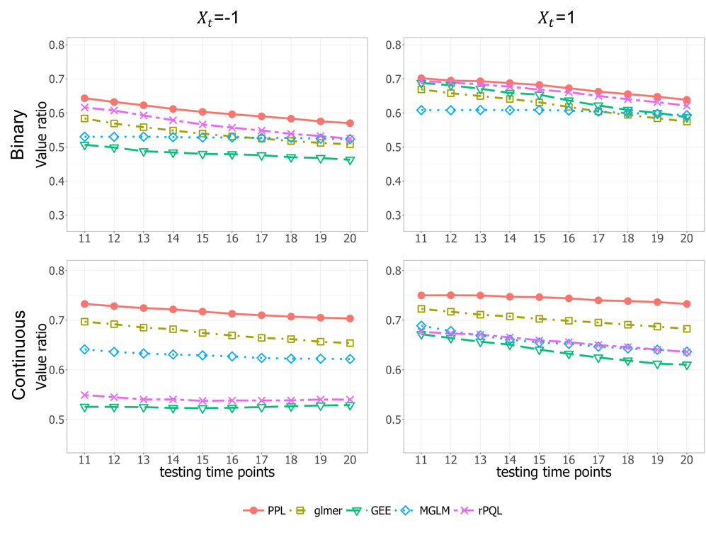
Figure 1: Value ratio at each testing time point in the simulation with $m=10$ under scenario with non-sparse random effects by different $X_{t}$.

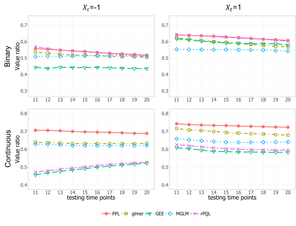
Figure 2: Value ratio at each testing time point in the simulation with $m=10$ under scenario with sparse random effects by different $X_{t}$.

5 Application

We apply the proposed PPL to estimate the best personalized push schedule in 294 users, who have received at least 20 prompts to complete the patient-health questionnaire since they downloaded the Hub app. Since the prompts were scheduled on 7-day intervals, this would represent a subsample of users with at least 20 weeks of app use. The distribution of the number of prompts in these users is shown in Figure 3. In the data, we tracked the timestamp of when a prompt was sent. For the purpose of this analysis, we grouped the time of prompt into four periods: Night ($a_{1}$): from midnight to 6:00am; Morning ($a_{2}$): from 6:00am to noon; Afternoon ($a_{3}$): from noon to 6:00pm; Evening ($a_{4}$): from 6:00pm to midnight. The observed proportions of the four periods were respectively 0.10, 0.23, 0.35, and 0.32. Using $a_{1}$ as the reference group, we used three dummy variables, centered by the observed proportions, to code the actions $a_{2},a_{3}$, and $a_{4}$ in model fitting.

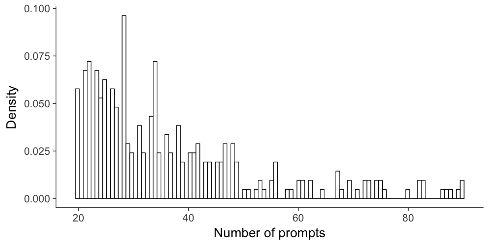
Figure 3: The distribution of the number of prompts in 294 IntelliCare users.

The state $S_{it}$ at each time point consisted of three variables. First, the number of times the Hub was launched (launches) in the week prior to the prompt was recorded. Second, the timestamp indicated whether a prompt was sent on a weekday (weekday). Third, the time point $t$ of the prompt was included as a predictor in the covariate process $S_{it}$. With a binary response outcome, we estimated $(\bm{\beta},\bm{\alpha})$ under model (1) with a logit link, $h_{1}(S,A)=(1,launches,t,weekday,A,launches\otimes A,weekday\otimes A,t\otimes A)$ and $h_{2}(S,A)=(1,A,launches\otimes A,weekday\otimes A,t\otimes A)$ using the first 80% of the time points of each user as training data. Since each user had at least 20 prompts, we had $m_{i}\geq 16$ in the training data for all 294 users.

Table 3 summarizes the results of the model fit. The positive fixed effects for $a_{2},a_{3},a_{4}$ suggest prompts in the morning, afternoon, and evening tend to induce better response rate than those sent during the night (midnight to 6:00am). The effects associated with these non-night periods are even greater on weekdays, indicated by the positive (fixed) interaction between weekday and these periods. While this result is not surprising, we also note substantial heterogeneity of the period effects and the $weekday$:period interactions, whose SD$(\hat{\bm{\alpha}})$s have comparable magnitude to $\hat{\bm{\beta}}$. This supports the needs for personalizing push schedule in our application.

In contrast, for the $launches$:period interactions and the $t$:period interactions, the fixed effects ($\hat{\bm{\beta}}$) dominate the random effects; heterogeneity of the random effects coefficients are measured by SD$(\hat{\bm{\alpha}})$. Based on the fixed effects, the response rate decreases over time, by 0.20 in log-odds over $t=5$ time points. This is in line with findings in the literature; see Helander et al., (2014) for example. In addition, every five additional launches of the Hub in the prior week improves the log-odds of response to a night prompt by $1.52$. Based on the negative coefficients of launches:period interactions, a large number of launches also seems to attenuate or even negate the effects of the time of prompts. This suggests that for active users who engage the Hub often, their response pattern is less sensitive to the time of the prompt.

Table 3: Model fit using the training data: $\hat{\bm{\beta}}$ is the coefficients of the fixed effects, and SD$(\hat{\bm{\alpha}})$ is the standard deviation of the fitted individual random effects coefficients.

Variables	$\hat{\bm{\beta}}$	SD$(\hat{\bm{\alpha}})$
$Intercept$	-1.80	1.31
$weekday$	0.01	—
$launches$ (per 5 times)	1.52	—
$t$ (per 5 time points)	-0.20	—
Morning ($a_{2}$)	1.65	1.13
Afternoon ($a_{3}$)	1.57	0.95
Evening ($a_{4}$)	1.06	0.78
$weekday:a_{2}$	0.73	0.34
$weekday:a_{3}$	0.16	0.62
$weekday:a_{4}$	0.66	0.52
$launches:a_{2}$	-2.46	0.39
$launches:a_{3}$	-1.40	0.21
$launches:a_{4}$	-1.15	0.43
$t:a_{2}$	- 1.25	0.66
$t:a_{3}$	-0.96	0.47
$t:a_{4}$	-0.93	0.44

The quality of these personalized policies in the testing data is evaluated by the mean response rate under the policies estimated via inverse probability treatment weighted method averaged over all test time points. The mean response rate according to PPL would have been 23%, which compares favorably to other studies in light of the fact that all testing points are at least 16 weeks from first download. It has been reported that user engagement is in the range of 3% to 15% in the third month after download (Helander et al.,, 2014). As a reference point, the observed response rate in the testing data is 11%. In addition, we analyzed the prompt response data using the other methods with the same 80%-20% split of training and testing data, and obtained the mean response rate 14%, 17%, 14%, and 8% respectively for glmer, GEE, MGLM, and rPQL.

6 Discussion

This article makes several contributions. First, we have shown personalized policies lead to higher value than non-personalized policy (i.e., GEE) in our simulation study, and have clearly demonstrated substantial heterogeneity of the action effects in the prompt response data. These results imply a paradigm shift and call for the necessity of personalized policies, which fundamentally differ from a single policy that may allow personalized decisions by tailoring. Second, we propose a novel computational algorithm for the estimation of model parameters under GLMM and for developing personalized policies. We have demonstrated, by simulation and in our data application, that the algorithm leads to better estimation properties and decision quality when compared to some existing methods, namely glmer and rPQL. Third, we have provided theoretical justifications of the proposed PPL by examining its asymptotic properties under a fairly general set of assumptions. In particular, we have established consistency and optimality in the presence of endogenous covariate process, where the covariates may depend on previous outcomes, actions, and even the latent random effects. As endogeneity is ubiquitous in longitudinal mobile application usage (how many times a user launched the Hub app would likely depend on how he/she had interacted with the Hub in the past), these theoretical results have broadened the applicability of PPL to many practical situations.

Appendix: Examples of endogenous covariates

In this section, we verify condition (C6) in two examples with endogenous covariates. In the first example, $Y_{it}$ is binary , and the distribution of $S_{it}$ directly depends on the random effects parameters $\bm{\alpha}_{0i\cdot}$. In the second example, $Y_{it}$ is Gaussian, and $S_{it}=Y_{i,t-1}$. For simplicity, we verify the condition with $n=1$ (since individuals are i.i.d.), and omit subscript $i$ from the notations. In both examples, we consider a scalar mean zero random effects parameter $\alpha_{0}\in\mathbb{R}$, and the treatment $A_{t}\in\{-1,1\}$ is randomly assigned with $P(A_{t}=1)=P(A_{t}=-1)=1/2$ for $t\geq 1$.

Example 1. For binary outcome $Y_{t}\in\{0,1\}$, suppose

$$g(E(Y_{t}|S_{t},A_{t}))=(\beta_{0}+\alpha_{0})S_{t}A_{t},$$

where $g(\cdot)$ is the logit link. Conditioning on $\alpha$, $S_{t},t=1,\ldots,m$, are i.i.d. $N(\alpha_{0},\tau^{2})$.

Let $\ell(Y_{t},S_{t},A_{t};\beta,\alpha)$ be the log-likelihood of Bermoulli distribution with mean $\frac{e^{(\beta+\alpha)S_{t}A_{t}}}{1+e^{(\beta+\alpha)S_{t}A_{t}}}$. Then $\ell_{1}(\beta,\alpha)=\sum_{t=1}^{m}\ell(Y_{t},S_{t},A_{t};\beta,\alpha)$ satisfies

$$\ell_{1}(\beta,\alpha) = \sum_{t=1}^{m}Y_{t}(\beta+\alpha)S_{t}A_{t}-\log\left\{1+e^{(\beta+\alpha)S_{t}A_{t}}\right\},$$

$$\nabla_{\beta}\ell_{1}(\beta,\alpha) = \nabla_{\alpha}\ell_{1}(\beta,\alpha)=\sum_{t=1}^{m}S_{t}A_{t}\left\{Y_{t}-\frac{e^{(\beta+\alpha)S_{t}A_{t}}}{1+e^{(\beta+\alpha)S_{t}A_{t}}}\right\},$$

$$\mbox{and }\nabla_{\beta}^{\intercal}\nabla_{\beta}\ell_{1}(\beta,\alpha) = \nabla_{\alpha}^{\intercal}\nabla_{\alpha}\ell_{1}(\beta,\alpha)=-\sum_{t=1}^{m}\frac{S_{t}^{2}e^{(\beta+\alpha)S_{t}A_{t}}}{\left\{1+e^{(\beta+\alpha)S_{t}A_{t}}\right\}^{2}}.$$

It is easy to verify that

$$E\left\{\nabla_{\beta}\ell_{1}(\beta_{0},\alpha_{0})\right\}=E\left\{\nabla_{\alpha}\ell_{1}(\beta_{0},\alpha_{0})\right\}=0,$$

$$\frac{1}{m}E\left[\left\{\nabla_{\beta}\ell_{1}(\beta_{0},\alpha_{0})\right\}^{2}\right]=\frac{1}{m}E\left[\left\{\nabla_{\alpha}\ell_{1}(\beta_{0},\alpha_{0})\right\}^{2}\right]$$

$$= \frac{1}{m}\sum_{t=1}^{m}E\left\{\frac{S_{t}^{2}e^{(\beta_{0}+\alpha_{0})S_{t}A_{t}}}{\left\{1+e^{(\beta_{0}+\alpha_{0})S_{t}A_{t}}\right\}^{2}}\right\}=E\left\{\frac{S_{1}^{2}e^{(\beta_{0}+\alpha_{0})S_{1}A_{1}}}{\left\{1+e^{(\beta_{0}+\alpha_{0})S_{1}A_{1}}\right\}^{2}}\right\}<\infty,$$

and

$$\bm{M}_{\beta\beta}=\bm{M}_{\alpha\alpha}=E\left\{\frac{S_{1}^{2}e^{(\beta_{0}+\alpha_{0})S_{1}A_{1}}}{\left\{1+e^{(\beta_{0}+\alpha_{0})S_{1}A_{1}}\right\}^{2}}\right\}>0.$$

Finally, conditioning on $\alpha_{0}$, $\left\{\frac{S_{t}^{2}e^{(\beta+\alpha)S_{t}A_{t}}}{\left\{1+e^{(\beta+\alpha)S_{t}A_{t}}\right\}^{2}},t=1,\ldots,m\right\}$ are i.i.d., where $\alpha=\alpha_{0}+u$. By the uniform law of large numbers theorem,

$$\sup_{(\beta,\alpha)\in\Omega}\left|m^{-1}\nabla_{\beta}^{\intercal}\nabla_{\beta}\ell_{1}(\beta,\alpha)-E\left\{\frac{S_{1}^{2}e^{(\beta+\alpha)S_{1}A_{1}}}{\left\{1+e^{(\beta+\alpha)S_{1}A_{1}}\right\}^{2}}\bigg{|}\alpha_{0}\right\}\right|=o_{P}(1).$$

Example 2. Suppose

$$Y_{t}|S_{t},A_{t},\beta_{0},\alpha_{0}\sim N\{(\beta_{0}+\alpha_{0})S_{t}A_{t},\sigma^{2}\},$$

where $S_{t}=Y_{t-1}$, and $Y_{0}\equiv\mu_{0}$ is a constant. We consider $l(\cdot)$ to be the log-likelihood of Gaussian distribution. Below we show that condition (C6) holds when

$$P_{\alpha_{0}}(|\beta_{0}+\alpha_{0}|<1)=1.$$ (9)

Note that condition (9) is a sufficient condition for an AR(1) process to be stationary.

$$\ell_{1}(\beta,\alpha) = -\frac{1}{2\sigma^{2}}\sum_{t=1}^{m}\left\{Y_{t}-(\beta+\alpha)Y_{t-1}A_{t}\right\}^{2},$$

$$\nabla_{\beta}\ell_{1}(\beta,\alpha) = \nabla_{\alpha}\ell_{1}(\beta,\alpha)=\frac{1}{\sigma^{2}}\sum_{t=1}^{m}\left\{Y_{t}-(\beta+\alpha)Y_{t-1}A_{t}\right\}Y_{t-1}A_{t},$$

$$\mbox{and }\nabla_{\beta}^{\intercal}\nabla_{\beta}\ell_{1}(\beta,\alpha) = \nabla_{\alpha}^{\intercal}\nabla_{\alpha}\ell_{1}(\beta,\alpha)=-\frac{1}{\sigma^{2}}\sum_{t=1}^{m}Y_{t-1}^{2}.$$

We can verify that

$$E\left\{\nabla_{\beta}\ell_{1}(\beta_{0},\alpha_{0})\right\}=E\left\{\nabla_{\alpha}\ell_{1}(\beta_{0},\alpha_{0})\right\}=0.$$

Noticing that $E(Y_{t}^{2})=\sum_{k=1}^{t-1}\sigma^{2}E\left\{(\beta_{0}+\alpha_{0})^{2(k-1)}\right\}$, we have,

$$\frac{1}{m}E\left[\left\{\nabla_{\beta}\ell_{1}(\beta_{0},\alpha_{0})\right\}^{2}\right]=\frac{1}{m}E\left[\left\{\nabla_{\alpha}\ell_{1}(\beta_{0},\alpha_{0})\right\}^{2}\right]$$

$$= \frac{1}{m\sigma^{2}}\sum_{t=1}^{m}E(Y_{t}^{2})=\frac{1}{m}\sum_{t=1}^{m}\sum_{k=1}^{t-1}E\left\{(\beta+\alpha)^{2(k-1)}\right\}$$

$$= \frac{1}{m}\sum_{t=1}^{m}(m-t+1)E\left\{(\beta_{0}+\alpha_{0})^{2(t-1)}\right\}$$

which is $O(1)$ when (9) holds.

Since $(m-t+1)E\left\{(\beta_{0}+\alpha_{0})^{2(t-1)}\right\}=m$ when $t=1$, we have

$$\bm{M}_{\beta\beta}=\bm{M}_{\alpha\alpha}=\frac{1}{m}\sum_{t=1}^{m}(m-t+1)E\left\{(\beta_{0}+\alpha_{0})^{2(t-1)}\right\}\geq 1.$$

Finally, under condition (9), for any $\epsilon>0$,

$$P\left\{\sup_{(\beta,\alpha^{\prime})\in\Omega}\left|\frac{1}{m}\sum_{t=1}^{m}Y_{t}^{2}-E(Y_{t}^{2}|\alpha_{0})\right|>\epsilon\bigg{|}\alpha_{0}\right\}$$

$$= P\left\{\left|\frac{1}{m}\sum_{t=1}^{m}Y_{t}^{2}-E(Y_{t}^{2}|\alpha_{0})\right|>\epsilon\bigg{|}\alpha_{0}\right\}$$

$$\leq (\epsilon m)^{-2}E\left[\sum_{t=1}^{m}\left\{Y_{t}^{2}-E(Y_{t}^{2}|\alpha_{0})\right\}\bigg{|}\alpha_{0}\right]^{2}$$

$$= (\epsilon m)^{-2}2\sigma^{4}\sum_{t=1}^{m}\sum_{k=1}^{t-1}(\beta_{0}+\alpha_{0})^{4(k-1)}+(\epsilon m)^{-2}4\sigma^{4}\sum_{t=1}^{m-1}\sum_{t^{\prime}=t+1}^{m}(\beta_{0}+\alpha_{0})^{2(t^{\prime}-t)}\sum_{l=0}^{2t-1}(\beta_{0}+\alpha_{0})^{2l}$$

$$= (\epsilon m)^{-2}O(m)=o(1),$$

which implies that

$$\sup_{(\beta,\alpha)\in\Omega}\left|m^{-1}\nabla_{\beta}^{\intercal}\nabla_{\beta}\ell_{1}(\beta,\alpha)-E\left\{m^{-1}\nabla_{\beta}^{\intercal}\nabla_{\beta}\ell_{1}(\beta,\alpha)|\alpha_{0}\right\}\right|=o_{P}(1).$$

SUPPLEMENTARY MATERIAL

Section S1 contains the estimation algorithm of policy parameters.

Section S2 contains proofs of all technical results.

Section S3 contains additional simulation results for decision quality comparison of the five methods when $m=20,30$.

References

- Bates et al., (2014) Bates, D., Mächler, M., Bolker, B., and Walker, S. (2014). Fitting linear mixed-effects models using lme4. arXiv preprint, arXiv:1406.5823.
- Bohmer et al., (2011) Bohmer, M., Hecht, B., Schoning, J., Kruger, A., and Bauer, G. (2011). Falling asleep with angry birds, facebook and kindle - a large scale study on mobile application usage. In MobileHCI, pages 47–56.
- Boruvka et al., (2018) Boruvka, A., Almirall, D., Witkiewitz, K., and Murphy, S. A. (2018). Assessing time-varying causal effect moderation in mobile health. Journal of the American Statistical Association, 113(523):1112–1121.
- Cheung et al., (2018) Cheung, K., Ling, W., Kar, r. C. J., Weingardt, K., Schueller, S. M., and Mohr, D. C. (2018). Evaluation of a recommender app for apps for the treatment of depression and anxiety: an analysis of longitudinal user engagement. Journal of the American Medical Informatics Association, 25(8):955–962.
- Cho et al., (2017) Cho, H., Wang, P., and Qu, A. (2017). Personalize treatment for longitudinal data using unspecified random-effects model. Statistica Sinica, 27:187–206.
- Christmann et al., (2009) Christmann, C. A., Hoffmann, A., and Bleser, G. (2009). Adherence in internet interventions for anxiety and depression. Journal of Medical Internet Research, 11(2):e13.
- Depp et al., (2010) Depp, C. A., Mausbach, B., Granholm, E., Cardenas, V., Ben-Zeev, D., Patterson, T. L., Lebowitz, B. D., and Jeste, D. V. (2010). Mobile interventions for severe mental illness: design and preliminary data from three approaches. The Journal of nervous and mental disease, 198(10):715.
- Diggle et al., (2002) Diggle, P., Heagerty, P., Liang, K.-Y., and Zeger, S. (2002). Analysis of longitudinal data. Oxford University Press.
- Ertefaie and Strawderman, (2018) Ertefaie, A. and Strawderman, R. L. (2018). Constructing dynamic treatment regimes over indefinite time horizons. Biometrika, 105(4):963–977.
- Helander et al., (2014) Helander, E., Kaipainen, K., Korhonen, I., and Wansink, B. (2014). Factors related to sustained use of a free mobile app for dietary self-monitoring with photography and peer feedback: retrospective cohort study. Journal of Medical Internet Research, 16(4):e109.
- Heron and Smyth, (2010) Heron, K. E. and Smyth, J. M. (2010). Ecological momentary interventions: incorporating mobile technology into psychosocial and health behaviour treatments. British journal of health psychology, 15(1):1–39.
- Hui et al., (2017) Hui, F. K., Müller, S., and Welsh, A. (2017). Joint selection in mixed models using regularized pql. Journal of the American Statistical Association, 112(519):1323–1333.
- Kravitz and Duan, (2014) Kravitz, R. and Duan, N. (2014). Design and implementation of n-of-1 trials: A user’s guide. Agency for Healthcare Research and Quality, 13(14).
- Laber et al., (2014) Laber, E., Linn, K., and Stefanski, L. (2014). Interactive model building for Q-learning. Biometrika, 101(4):831–847.
- Lei et al., (2017) Lei, H., Tewari, A., and Murphy, S. (2017). An actor-critic contextual bandit algorithm for personalized interventions using mobile devices. arXiv Preprint, arXiv:1706.09090.
- Lillie et al., (2011) Lillie, E., Patay, B., Diamant, J., Issell, B., Topol, E., and Schork, N. (2011). The n-of-1 clinical trial: the ultimate strategy for individualizing medicine. Personalized Medicine, 8(2):161–173.
- Luckett et al., (2019) Luckett, D. J., Laber, E. B., Kahkoska, A. R., Maahs, D. M., Mayer-Davis, E., and Kosorok, M. R. (2019). Estimating dynamic treatment regimes in mobile health using v-learning. Journal of the American Statistical Association, (just-accepted):1–39.
- Mohr et al., (2013) Mohr, D. C., Cheung, K., Schueller, S. M., Brown, C. H., and Duan, N. (2013). Continuous evaluation of evolving behavioral intervention technologies. American Journal of Preventive Medicine, 45(4):517–523.
- Mohr et al., (2017) Mohr, D. C., Tomasino, K. N., Lattie, E. G., Palac, H. L., Kwasny, M. J., Weingardt, K., Karr, C. J., Kaiser, S. M., Rossom, R. C., Bardsley, L. R., et al. (2017). Intellicare: an eclectic, skills-based app suite for the treatment of depression and anxiety. Journal of Medical Internet Research, 19(1):e10.
- Murphy, (2003) Murphy, S. A. (2003). Optimal dynamic treatment regimes. Journal of the Royal Statistical Society: Series B (Statistical Methodology), 65(2):331–355.
- Nash, (2000) Nash, S. G. (2000). A survey of truncated-newton methods. Journal of Computational and Applied Mathematics, 124(1-2):45–59.
- Ohrnberger et al., (2017) Ohrnberger, J., Fichera, E., and Sutton, M. (2017). The rise of consumer health wearables: promises and barriers. Journal of the Economics of Ageing, 9:52–62.
- Pepe and Anderson, (1994) Pepe, M. S. and Anderson, G. L. (1994). A cautionary note on inference for marginal regression models with longitudinal data and general correlated response data. Communications in Statistics-Simulation and Computation, 23(4):939–951.
- Qian and Murphy, (2011) Qian, M. and Murphy, S. A. (2011). Performance guarantees for individualized treatment rules. Annals of Statistics, 39(2):1180–1210.
- Qian et al., (2019) Qian, T., Klasnja, P., and Murphy, S. A. (2019). Linear mixed models under endogeneity: modeling sequential treatment effects with application to a mobile health study. arXiv:1902.10861.
- Riley et al., (2011) Riley, W. T., Rivera, D. E., Atienza, A. A., Nilsen, W., Allison, S. M., and Mermelstein, R. (2011). Health behavior models in the age of mobile interventions: are our theories up to the task? Translational Behavioral Medicine, 1(1):53–71.
- Song et al., (2015) Song, R., Wang, W., Zeng, D., and Kosorok, M. R. (2015). Penalized q-learning for dynamic treatment regimes. Statistical Sinica, 25(3):901–920.
- Steihaug, (1983) Steihaug, T. (1983). The conjugate gradient method and trust regions in large scale optimization. SIAM Journal on Numerical Analysis, 20(3):626–637.
- Yuan and Lin, (2006) Yuan, M. and Lin, Y. (2006). Model selection and estimation in regression with grouped variables. Journal of the Royal Statistical Society: Series B (Statistical Methodology), 68(1):49–67.
- Zhang et al., (2012) Zhang, B., Tsiatis, A. A., Laber, E. B., and Davidian, M. (2012). A robust method for estimating optimal treatment regimes. Biometrics, 68(4):1010–1018.
- Zhao et al., (2015) Zhao, Y., Zeng, D., Laber, E. B., and Kosorok, M. R. (2015). New statistical learning methods for estimating optimal dynamic treatment regimes. Journal of the American Statistical Association, 110(510):583–598.
- Zhao et al., (2012) Zhao, Y., Zeng, D., Rush, A. J., and Kosorok, M. R. (2012). Estimating individualized treatment rules using outcome weighted learning. Journal of the American Statistical Association, 107(499):1106–1118.