Energy-Minimizing Bit Allocation For Powerline OFDM With Multiple Delay Constraints

Abstract

We propose a bit-allocation scheme for powerline orthogonal frequency-division multiplexing (OFDM) that minimizes total transmit energy subject to total-bit and delay constraints. Multiple delay requirements stem from different sets of data that a transmitter must time-multiplex and transmit to a receiver. The proposed bit allocation takes into account the channel power-to-noise density ratio of subchannels as well as statistic of narrowband interference and impulsive noise that is pervasive in powerline communication (PLC) channels. The proposed scheme is optimal with 1 or 2 sets of data, and is suboptimal with more than 2 sets of data. However, numerical examples show that the proposed scheme performs close to the optimum. Also, it is less computationally complex than the optimal scheme especially when minimizing total energy over large number of data sets. We also compare the proposed scheme with some existing schemes and find that our scheme requires less total transmit energy when the number of delay constraints is large.

1 Introduction

Existing electrical wiring makes powerline communication (PLC) an enticing technology for home or in-car networking due to cost reduction in wire installation and for hospitals due to absence of radio-frequency transmission that could interfere with medical instruments. In IEEE 1901 standard, which stipulates broadband transmission over powerlines [1], orthogonal frequency-division multiplexing (OFDM) is applied to transmit data over subchannels. However, designing and optimizing OFDM transmission require the PLC channel models that accurately reflect the characteristics of the actual channels. The work by [2] has proposed the powerline channel models, which are widely used to analyze the performance of data transmission over PLC channels. The models account for both signal attenuation and multipath propagation due to impedance mismatching of electrical components. In addition to colored background noise, impulsive noise caused by power-supply switching must also be considered when designing PLC transmission schemes [3]. Whenever impulsive noise occurs, its power could exceed 50 dB above that of the background noise [4]. The other potential impediment to PLC transmission is narrowband interference caused by short-wave or medium-wave radio transmitters with a frequency range between 300 kHz and 3 MHz [5].

Optimizing bit, subcarrier, and power allocation for both wired and wireless OFDM have been considered by many works [6, 7, 8, 9, 10, 11, 12, 13]. In [6], subcarrier and power allocation scheme was proposed to maximize sum rate of all users, subject to proportional rate constraint. The work by [7] proposed an adaptive power loading to minimize the transmit power, subject to a fixed bit rate and maximum bit error rate (BER). For PLC channels, several work [8, 9, 10, 11, 12, 13] consider resource allocation at the transmitter with varying objectives. In [8, 11], throughput is maximized with constraints on total power or BER while in [9], outage probability is minimized with a target BER. In [10], the maximum transmission time of all subchannels is minimized for a Zimmermann channel model [2], subject to a total-energy constraint. In [12], bit-loading with a single delay constraint is performed on OFDM channels to minimize transmission energy. The work by [13] proposed subchannel and bit allocation for multiple users to minimize transmission power under transmit rate constraints.

The aim of this work is to minimize transmit energy in PLC OFDM channels. Differing particularly from [13, 10, 12] and other existing work, our proposed bit allocation is applied to a transmitter under multiple delay constraints. In our problem formulation, a transmitter must time-multiplex different sets of data with varying delay and total-bit constraints and then distributes them over OFDM subchannels. Each set of data may arise from different users or classes of service that share the same channel. For two delay constraints, we derive the optimal bit allocation over OFDM subchannels and the optimal transmit durations that minimize the total transmit energy. With three or more delay constraints, we propose a suboptimal allocation that iterates the optimal 2-delay solution and show via numerical results that the proposed suboptimal allocation performs close to the optimum. With numerical examples, we compare our proposed scheme with that by [13] and show that our scheme attains lower transmit energy when the number of delay constraints and the number of transmitted bits are large. The proposed scheme also has much lower computational complexity than the optimum does especially for a large number of delay constraints.

2 System Model and Problem Statement

We assume OFDM with $N$ subchannels and that transmitter has $K$ different sets of data with various sizes and delay requirements to transmit over time-division multiplexing (TDM) network. For the $k$th data set on the $n$th subchannel, the discrete-time received symbol is given by

$$r_{n,k}=\sqrt{P_{n,k}}H_{n}x_{n,k}+w_{n,k}$$ (1)

where $x_{n,k}$ is a transmitted symbol with zero mean and unit variance, $H_{n}$ is a complex frequency response of the $n$th subchannel, $P_{n,k}$ is a transmission power for the $k$th set of data in the $n$th subchannel, and $w_{n,k}$ is a background noise over the $n$th subchannel for the $k$th data set. We assume that channel response is relatively static during the transmission of the current data sets and thus, frequency response $H_{n}$ does not depend on the index $k$. In other words, the channel’s coherent time is sufficiently long that optimizing the transmission is meaningful. The considered channel might correspond to a large PLC network in which the dynamics of a few nodes do not alter channel response drastically.

In addition to background noise, PLC channels suffer high-energy impulsive noise, which is peaky in time domain, and narrowband interference in some environment. During an instance of impulsive noise or narrowband interference, the receiver is not able to reliably decode the received symbols. Thus, the associated achievable rate during that instance is reduced to zero. We denote the probability of impulsive noise and/or narrowband interference occurrence in subchannel $n$ by $p_{n}$. While each instance of impulsive noise affects almost all subchannels, narrowband interference from short-wave or medium-wave radio only affects a few subchannels. Thus, $p_{n}$ may not be the same for all subchannels.

With probability $1-p_{n}$, the achievable rate in bits per second per Hertz for subchannel $n$ is given by

$$C_{n,k}=\log_{2}\left(1+\frac{J_{n,k}|H_{n}|^{2}}{t_{k}B\eta_{n}}\right)$$ (2)

where $B$ is a subchannel spacing, $\eta_{n}$ is the noise’s power spectral density (PSD) of the $n$th subchannel, $t_{k}$ denotes a transmit duration for the $k$th set of data, and $J_{n,k}$ is the energy used to transmit data for that duration on the $n$th subchannel. Hence, the average number of bits transmitted via the $n$th subchannel is given by

$$\bar{Q}_{n,k} =E[C_{n,k}]t_{k}B$$ (3)

$$=(1-p_{n})t_{k}B\log_{2}\left(1+\frac{J_{n,k}}{t_{k}BG_{n}}\right)$$ (4)

where $G_{n}\triangleq\frac{\eta_{n}}{|H_{n}|^{2}}$ is an inverse of channel power-to-noise density ratio (CNR) for subchannel $n$. The energy required to transmit average $\bar{Q}_{n,k}$ bits can be computed by

$$J_{n,k}=(2^{\frac{\bar{Q}_{n,k}}{(1-p_{n})t_{k}B}}-1)t_{k}BG_{n}.$$ (5)

Assuming that the $k$th set of data consists of total average $Q_{k}$ bits, the sum of all bits for the $k$th set over all OFDM subchannels must equal or exceed $Q_{k}$

$$\sum_{n=1}^{N}\bar{Q}_{n,k}\geq Q_{k},\quad\text{for}\ 1\leq k\leq K,$$ (6)

while the total energy associated with the $k$th transmission is given by $\sum_{n=1}^{N}J_{n,k}$. We note that the transmit duration for the $k$th set of data must not exceed its delay requirement $T_{k}>0$. Without loss of generality, sets of data are ordered according to the required delay in an increasing order. Thus, $T_{1}\leq T_{2}\leq\ldots\leq T_{K}$. With that transmission order, the delay constraint for the $k$th set can be expressed as follows

$$\sum_{i=1}^{k}t_{i}\leq T_{k},\quad\text{for}\ 1\leq k\leq K.$$ (7)

In other words, the cumulative transmission time up to and including the $k$th transmission must not exceed $T_{k}$. In this work, we would like to allocate average bits $\{\bar{Q}_{n,k}\}$ over $N$ available subchannels and transmit durations $\{t_{k}\}$ for all $K$ sets of data to minimize the total transmit energy

$$\min_{\{\bar{Q}_{n,k}\},\{t_{k}\}}J\triangleq\sum_{k=1}^{K}\sum_{n=1}^{N}J_{n,k}$$ (8)

subject to total-average-bit and delay constraints in (6) and (7), respectively.

3 Proposed Bit-Allocation Scheme

First, we consider problem (8) with $K=2$. We remark that bit allocation with single data set ($K=1$) that minimizes transmit energy, has been solved by our previous work [12]. Since the objective function in (8) is convex with $\bar{Q}_{n,1},\,\bar{Q}_{n,2}\geq 0,\forall n$, and $t_{1},\,t_{2}\geq 0$, while both constraints (6) and (7) are linear with those same variables, the solutions that satisfy the Kuhn-Tucker conditions are optimal. To derive the Kuhn-Tucker conditions [14], we first form a Lagrangian as follows

$$\mathcal{L}=\sum_{n=1}^{N}(J_{n,1}+J_{n,2})+\beta_{1}(t_{1}-T_{1})+\beta_{2}(t_{1}+t_{2}-T_{2})\\ -\lambda_{1}(\sum_{n=1}^{N}\bar{Q}_{n,1}-{Q_{1}})-\lambda_{2}(\sum_{n=1}^{N}\bar{Q}_{n,2}-{Q_{2}})$$ (9)

where $\beta_{1}$, $\beta_{2}$, $\lambda_{1}$, and $\lambda_{2}$ are Lagrange multipliers associated with constraints (7) and (6), respectively. The Kuhn-Tucker conditions associated with the average bits $\bar{Q}_{n,k}$ and total-bit constraints are given by

$$\frac{\partial\mathcal{L}}{\partial\bar{Q}_{n,k}}=2^{\frac{\bar{Q}_{n,k}}{(1-p_{n})t_{k}B}}\frac{\ln(2)G_{n}}{(1-p_{n})}-\lambda_{k}\geq 0,$$ (10)

$$\bar{Q}_{n,k}\geq 0,$$ (11)

$$\bar{Q}_{n,k}\frac{\partial\mathcal{L}}{\partial\bar{Q}_{n,k}}=0,$$ (12)

for $k=1$ and $2$, and $1\leq n\leq N$, and

$$\frac{\partial\mathcal{L}}{\partial\lambda_{k}}=-\sum_{n=1}^{N}\bar{Q}_{n,k}+Q_{k}\leq 0,$$ (13)

$$\lambda_{k}\geq 0,$$ (14)

$$\lambda_{k}\frac{\partial\mathcal{L}}{\partial\lambda_{k}}=0,$$ (15)

for $k=1$ and $2$.

If subchannel $n$ of set $k$ is active or $\bar{Q}_{n,k}>0$, equations (10)-(12) imply

$$\lambda_{k}=2^{\frac{\bar{Q}_{n,k}}{(1-p_{n})t_{k}B}}\frac{\ln(2)G_{n}}{(1-p_{n})}.$$ (16)

But, if that subchannel is not used for transmission or $\bar{Q}_{n,k}=0$,

$$\lambda_{k}-2^{\frac{\bar{Q}_{n,k}}{(1-p_{n})t_{k}B}}\frac{\ln(2)G_{n}}{(1-p_{n})}<0.$$ (17)

For the first set of data ($k=1$), we can solve for the optimal bit allocation from (16) and (17) for some transmit duration $0<t_{1}\leq T_{1}$ as follows

$$\bar{Q}_{n,1}=Bt_{1}(1-p_{n})\\ \times\log_{2}\left(1+\left(\frac{1-p_{n}}{G_{n}\ln(2)}\lambda_{1}-1\right)^{+}\right)$$ (18)

where a positive-part function $x^{+}=\max\{x,0\}$. Hence, if $G_{n}\ln(2)/(1-p_{n})<\lambda_{1}$, the bit allocation in subchannel $n$ is nonzero or that subchannel is active. Given $t_{1}$, the bit allocation for each subchannel depends on $G_{n}/(1-p_{n})$ and threshold $\lambda_{1}$. If the quality of the subchannel is good ($G_{n}$ is small), the bit allocation $\bar{Q}_{n,1}$ will be large. However, if the quality of the subchannel is so poor that $G_{n}\ln(2)/(1-p_{n})<\lambda_{1}$, then that subchannel will not be active and will be allocated zero bits. Thus, $\lambda_{1}$ is the threshold that activates subchannels to transmit the first set of data. The threshold $\lambda_{1}$ can be determined from the total-bit constraint, which is obtained by summing (18) over all subchannels as follows

$$B\sum_{n=1}^{N}(1-p_{n})\log_{2}\left(1+\left(\frac{1-p_{n}}{G_{n}\ln(2)}\lambda_{1}-1\right)^{+}\right)\\ =\frac{Q_{1}}{t_{1}}.$$ (19)

Note that solving for $\lambda_{1}$ and $\{\bar{Q}_{n,1}\}$ gives water filling-like solutions. However, these solutions are not the same as the classical power allocation that maximizes sum capacity. We see from (19) that $\lambda_{1}$ increases with the transmission rate $Q_{1}/t_{1}$. Hence, if $Q_{1}/t_{1}$ is large enough, all subchannels can be active.

The threshold $\lambda_{1}$ can be solved from implicit equation (19). However, if the number of active subchannels is known, we can explicitly solve for $\lambda_{1}$ from (19) as follows

$$\log_{2}(\lambda_{1})=\frac{\frac{Q_{1}}{t_{1}B}-\sum_{n\in\mathbb{N}^{\mathrm{on}}_{1}}(1-p_{n})\log_{2}\left(\frac{1-p_{n}}{G_{n}\ln(2)}\right)}{\sum_{n\in\mathbb{N}^{\mathrm{on}}_{1}}1-p_{n}}$$ (20)

where $\mathbb{N}^{\mathrm{on}}_{1}\subset\{1,2,\dots,N\}$ is the set of active subchannels transmitting the first set of data. With (20), we propose the following iterations in Algorithm 1 to find the optimal $\lambda_{1}$ or $\lambda_{2}$. For each set of data, the algorithm takes at most $N$ iterations to find the optimal threshold $\lambda_{k}$ and the set of active subchannels $\mathbb{N}^{\mathrm{on}}_{k}$.

For a single set of data ($K=1$), we set input $t_{1}$ equal to $T_{1}$ in Algorithm 1, which will find the optimal bit allocation $\{Q_{n,1}\}$ for all $n$ and the optimal threshold $\lambda_{1}$. In the case that $K=1$ and the probability of impulsive noise or interference occurring in a subchannel is the same for all subchannels, Algorithm 1 reverts back to the bit allocation proposed in our previous work [12]. Regarding computational complexity, the algorithm takes at most $N$ iterations to find the optimal threshold $\lambda_{k}$ and the set of active subchannels $\mathbb{N}^{\mathrm{on}}_{k}$ for each set of data.

Algorithm 1 Finding the optimal thresholds and bit allocation for the $k$th data set

1:$Q_{k}$, $t_{k}$, $B$, $\{G_{n}\}$, and $\{p_{n}\}$.

2:Initialize: $\mathbb{N}^{\mathrm{on}}_{k}[0]=\{1,2,...,N\}$ and $i=0$

3:repeat

4:     $i\leftarrow i+1$

5:     $\mathbb{N}^{\mathrm{on}}_{k}[i]\leftarrow\mathbb{N}^{\mathrm{on}}_{k}[i-1]$

6:     Compute $\lambda_{k}$ from (20).

7:     for $n\in\mathbb{N}^{\mathrm{on}}_{k}[i]$ do

8:         Compute $\bar{Q}_{n,k}$ from (18).

9:         if $\bar{Q}_{n,k}=0$ then $\mathbb{N}^{\mathrm{on}}_{k}[i]\leftarrow\mathbb{N}^{\mathrm{on}}_{k}[i]\backslash\{n\}$

10:         end if

11:     end for

12:until $\mathbb{N}^{\mathrm{on}}_{k}[i]=\mathbb{N}^{\mathrm{on}}_{k}[i-1]$

13:return $\lambda_{k}$ and $\{\bar{Q}_{1,k},\bar{Q}_{2,k},\ldots,\bar{Q}_{N,k}\}$

To find the optimal transmit durations for 2 data sets ($K=2$), we derive the corresponding Kuhn-Tucker conditions for $t_{1}$ and $t_{2}$ given by

$$\frac{\partial\mathcal{L}}{\partial t_{k}}=\sum_{n=1}^{N}\bigg{[}(2^{\frac{\bar{Q}_{n,k}}{(1-p_{n})t_{k}B}}-1)BG_{n}\\ -2^{\frac{\bar{Q}_{n,k}}{(1-p_{n})t_{k}B}}\frac{\bar{Q}_{n,k}G_{n}\ln(2)}{(1-p_{n})t_{k}}\bigg{]}-\sum_{i=k}^{K}\beta_{i}\geq 0,$$ (21)

$$t_{k}\geq 0,$$ (22)

$$t_{k}\frac{\partial\mathcal{L}}{\partial t_{k}}=0,$$ (23)

for $k=1$ and $2$. Since $t_{k}>0$, $\partial\mathcal{L}/\partial t_{k}=0$. Substitute (16) in (21) to obtain

$$\lambda_{k}\left(\frac{B}{\ln(2)}\sum_{n\in\mathbb{N}^{\mathrm{on}}_{k}}(1-p_{n})-\frac{Q_{k}}{t_{k}}\right)\\ -B\sum_{n\in\mathbb{N}^{\mathrm{on}}_{k}}G_{n}-\sum_{i=k}^{K}\beta_{i}=0.$$ (24)

The Kuhn-Tucker conditions for Lagrange multipliers $\beta_{1}$ and $\beta_{2}$ are given by

$$\frac{\partial\mathcal{L}}{\partial\beta_{k}}=T_{k}-\sum_{i=1}^{k}t_{i}\geq 0,$$ (25)

$$\beta_{k}\geq 0,$$ (26)

$$\beta_{k}\frac{\partial\mathcal{L}}{\partial\beta_{k}}=0,$$ (27)

for $k=1$ and $2$. Since the second delay constraint is always tight or $t_{2}=T_{2}-t_{1}$, the associated Lagrange multiplier $\beta_{2}>0$ is given by

$$\beta_{2}=\lambda_{2}\left(\frac{B}{\ln(2)}\sum_{m\in\mathbb{N}^{\mathrm{on}}_{2}}(1-p_{m})-\frac{Q_{2}}{t_{2}}\right)\\ -B\sum_{m\in\mathbb{N}^{\mathrm{on}}_{2}}G_{m}.$$ (28)

Note that $\beta_{2}$ is a function of the rate $Q_{2}/t_{2}$, $\lambda_{2}$, and $\mathbb{N}^{\mathrm{on}}_{2}$. The last two parameters can be computed by Algorithm 1.

Similarly, if the delay constraint for the first set is tight or $t_{1}=T_{1}$, then $\beta_{1}>0$. However, if $t_{1}<T_{1}$, then $\beta_{1}=0$ where

$$\beta_{1}=\lambda_{1}\left(\frac{B}{\ln(2)}\sum_{n\in\mathbb{N}^{\mathrm{on}}_{1}}(1-p_{n})-\frac{Q_{1}}{t_{1}}\right)\\ -B\sum_{n\in\mathbb{N}^{\mathrm{on}}_{1}}G_{n}-\beta_{2}.$$ (29)

Given $t_{1}$, $\beta_{1}$ can be computed by (29) in conjunction with (28) and Algorithm 1. If the optimal $t_{1}<T_{1}$, there must exist at least one value of $t_{1}\in(0,T_{1})$ that results in $\beta_{1}=0$. Thus, instead of a brute-force search of $t_{1}$, we propose to perform binary search or bisection method [15] with a target accuracy $\delta>0$ set to be very small. For each iteration, the interval for $t_{1}$ is halved until $|\beta_{1}|<\delta$. After $t_{1}$ is found, we can compute $t_{2}=T_{2}-t_{1}$. Finally, the optimal transmit durations and bit allocation for the 2 data sets are obtained. We summarize the steps in Algorithm 2.

If the maximum delay for the first data set has not been reached or $t_{1}<T_{1}$, then $\beta_{1}=0$ and thus, combining (28) and (29) eliminates $\beta_{2}$. Since (20) shows that $\lambda_{k}$ is also a function of $Q_{k}/t_{k}$, we can show that $Q_{1}/t_{1}=Q_{2}/t_{2}$. This also holds true for $K>2$. Therefore, we conclude that if delay constraints are not too restricting, the data rates $Q_{k}/t_{k}$ obtained from the proposed scheme will be equal for all users.

Algorithm 2 Optimal transmit duration and bit allocation over subchannels for 2 sets of data

1:$Q_{1},Q_{2},T_{1},T_{2}$ where $0<T_{1}\leq T_{2}$, $B$, $\{G_{n}\}$, and $\{p_{n}\}$.

2:Set accuracy $\delta\ll 1$.

3:$t_{1}\leftarrow T_{1}$

4:Compute $\lambda_{1}$ and $\{\bar{Q}_{n,1}\}$ with Algorithm 1.

5:$t_{2}\leftarrow T_{2}-t_{1}$

6:Compute $\lambda_{2}$ and $\{\bar{Q}_{n,2}\}$ with Algorithm 1.

7:Compute $\beta_{2}$ and $\beta_{1}$ from (28) and (29).

8:if $\beta_{1}>0$ and $\beta_{2}>0$ then

9:     return $t_{1}$, $t_{2}$, $\{Q_{n,1}\}$, and $\{Q_{n,2}\}$

10:else

11:     $t_{l}\leftarrow 0$ and $t_{r}\leftarrow T_{1}$

12:     repeat

13:         $t_{1}\leftarrow\frac{t_{l}+t_{r}}{2}$

14:         Compute $\lambda_{1}$ and $\{\bar{Q}_{n,1}\}$ with Algorithm 1.

15:         $t_{2}\leftarrow T_{2}-t_{1}$

16:         Compute $\lambda_{2}$ and $\{\bar{Q}_{n,2}\}$ with Algorithm 1.

17:         Compute $\beta_{2}$ and $\beta_{1}$ from (28) and (29).

18:         if $\beta_{1}>0$ then

19:              $t_{l}\leftarrow t_{1}$

20:         else

21:              $t_{r}\leftarrow t_{1}$

22:         end if

23:     until $|\beta_{1}|<\delta$ and $\beta_{2}>0$

24:     return $t_{1}$, $t_{2}$, $\{\bar{Q}_{n,1}\}$, and $\{\bar{Q}_{n,2}\}$

25:end if

For problem (8) with the number of delay constraints $K>2$, the associated Lagrangian is given by

$$\mathcal{L}=\sum_{k=1}^{K}\sum_{n=1}^{N}J_{n,k}-\sum_{k=1}^{K}\lambda_{k}(\sum_{n=1}^{N}\bar{Q}_{n,k}-{Q_{k}})\\ +\sum_{k=1}^{K}\beta_{k}(\sum_{i=1}^{k}t_{i}-T_{k})$$ (30)

where $\lambda_{k}$ and $\beta_{k}$ denote Lagrange multipliers associated with constraints (6) and (7), respectively. Similar to the problem with $K=2$, the Kuhn-Tucker conditions can be obtained. The threshold $\lambda_{k}$ can be determined from the total-bit constraint as follows

$$B\sum_{n=1}^{N}(1-p_{n})\log_{2}\left(1+\left(\frac{1-p_{n}}{G_{n}\ln(2)}\lambda_{k}-1\right)^{+}\right)\\ =\frac{Q_{k}}{t_{k}}.$$ (31)

Given the rate $Q_{k}/t_{k}$, we can solve for $\lambda_{k}$, which is the water level that determines the set of active subchannels for set $k$ denoted by $\mathbb{N}^{\mathrm{on}}_{k}$. If a subchannel is active, the average number of allocated bits for that subchannel is given by

$$\bar{Q}_{n,k}=Bt_{k}(1-p_{n})\\ \times\log_{2}\left(1+\left(\frac{1-p_{n}}{G_{n}\ln(2)}\lambda_{k}-1\right)^{+}\right).$$ (32)

Since the last delay constraint is always tight or $t_{K}=T_{K}-\sum_{k=1}^{K-1}t_{k}$, $\beta_{K}>0$ and is given by

$$\beta_{K}=\lambda_{K}\left(\frac{B}{\ln(2)}\sum_{m\in\mathbb{N}^{\mathrm{on}}_{K}}(1-p_{m})-\frac{Q_{K}}{t_{K}}\right)\\ -B\sum_{m\in\mathbb{N}^{\mathrm{on}}_{K}}G_{m}.$$ (33)

For other data sets $k\neq K$, if the delay constraint of that set is tight or $\sum_{i=1}^{k}t_{i}=T_{k}$, then $\beta_{k}>0$. Otherwise, $\beta_{k}=0$ where

$$\beta_{k}=\lambda_{k}\left(\frac{B}{\ln(2)}\sum_{n\in\mathbb{N}^{\mathrm{on}}_{k}}(1-p_{n})-\frac{Q_{k}}{t_{k}}\right)\\ -B\sum_{n\in\mathbb{N}^{\mathrm{on}}_{k}}G_{n}-\sum_{i=k+1}^{K}\beta_{i},\quad\forall k\neq K.$$ (34)

Finding the set of optimal transmit durations $\{t_{k}\}$ involves solving a nonlinear system with (25)-(27), (31), and (33)-(34) totaling $5K$ equations, and $3K$ unknowns including the sets of Lagrange multipliers $\{\beta_{k}\}$ and $\{\lambda_{k}\}$. Once the optimal $\{t_{k}\}$ is obtained, bit allocation across subchannels for all sets can be computed by (32). However, solving for $\{t_{k}\}$ is exceedingly complex for a very large $K$.

For a simpler allocation scheme with comparable performance, we propose Algorithm 3, which iteratively applies the optimal solutions for two delay constraints ($K=2$) derived earlier. The proposed scheme is executed as follows. First, we set $\mathsf{Q}_{1}=\sum_{k=1}^{K-1}Q_{k}$ and $\mathsf{Q}_{2}=Q_{K}$, and $\mathsf{T}_{1}=T_{K-1}$ and $\mathsf{T}_{2}=T_{K}$. With $\mathsf{Q}_{1}$, $\mathsf{Q}_{2}$, $\mathsf{T}_{1}$, and $\mathsf{T}_{2}$, we apply Algorithm 2, which returns $\{\bar{\mathsf{Q}}_{n,1}\}$, $\{\bar{\mathsf{Q}}_{n,2}\}$, $\forall n$, $\mathsf{t}_{1}$, and $\mathsf{t}_{2}$. We obtain the transmit duration for the last or the $K$th data set, $t_{K}=\mathsf{t}_{2}$, and the bit allocation for the $K$th set on subchannel $n$, $\bar{Q}_{n,K}=\mathsf{Q}_{n,2}$ for $1\leq n\leq N$. To find the allocation for the $(K-1)$th set, we apply Algorithm 2 with $\mathsf{Q}_{1}=\sum_{k=1}^{K-2}Q_{k}$ and $\mathsf{Q}_{2}=Q_{K-1}$, and $\mathsf{T}_{1}=T_{K-2}$ and $\mathsf{T}_{2}=T_{K-1}$. We iterate these steps for other $K-2$ rounds or until all bit allocation and transmit durations are obtained. All steps are shown in Algorithm 3. The computational complexity of this proposed suboptimal scheme increases only linearly with $K$ and is much less than that of solving for the optimum. Moreover, numerical results will show that these suboptimal solutions perform close to the optimum.

Algorithm 3 The proposed scheme that finds transmit durations and bit allocation over subchannels for the number of delay constraints $K\geq 1$.

1:$\{Q_{k}\}$, $\{T_{k}\}$ where $0<T_{1}\leq T_{2}\leq...\leq T_{K}$, $B$, $\{G_{n}\}$, and $\{p_{n}\}$.

2:if $K>1$ then

3:     repeat

4:         $\mathsf{T}_{1}=T_{K-1}$

5:         $\mathsf{T}_{2}=T_{K}$

6:         $\mathsf{Q}_{1}=\sum_{k=1}^{K-1}Q_{k}$

7:         $\mathsf{Q}_{2}=Q_{K}$

8:         Compute $\mathsf{t}_{1}$, $\mathsf{t}_{2}$, $\{\bar{\mathsf{Q}}_{n,1}\}$, and $\{\bar{\mathsf{Q}}_{n,2}\}$ by Algorithm 2 with inputs $\mathsf{T}_{1}$, $\mathsf{T}_{2}$, $\mathsf{Q}_{1}$, and $\mathsf{Q}_{2}$, and channel parameters $B$, $\{G_{n}\}$, and $\{p_{n}\}$.

9:         $t_{K}\leftarrow\mathsf{t}_{2}$

10:         $\{\bar{Q}_{n,K}\}\leftarrow\{\bar{\mathsf{Q}}_{n,2}\}$ for all $n$

11:         $K\leftarrow K-1$

12:     until $K=1$

13:end if

14:$t_{1}\leftarrow T_{1}$

15:Compute $\{\bar{Q}_{n,1}\}$ by Algorithm 1 with $Q_{1}$, and channel parameters $B$, $\{G_{n}\}$, and $\{p_{n}\}$.

16:return $t_{1},t_{2},\ldots,t_{K}$, and $\{\bar{Q}_{n,1}\},\{\bar{Q}_{n,2}\},\ldots,\{\bar{Q}_{n,K}\}$

4 Numerical Results

To generate numerical results, we utilize a frequency response of the 15-path channel model from [2], which was obtained by measuring and approximating from the actual powerline network. The measured network consists of a 110-meter link installed in an estate of terraced houses with six 15-meter branches. A link between two points in the network consists of a distributor cable or a series connection of distributor cables. The signal propagated along the line-of-sight path and non line-of-sight paths as echoes. Cable loss due to the length of signal propagation and frequency is also captured in the model.

For PSD of the background noise, the worst case in [16, Fig. 2] is assumed. Typically, the probability of impulsive noise is less than 5% even in a highly disturbed PLC network [4]. Assuming the worst-case probability, $p_{n}$ is at least equal to 0.05. Additionally, subchannels in a frequency range of short-wave or medium-wave radio can be interfered by those radio transmitters. Thus, we assume $p_{n}=0.06$ in those subchannels accounting for interference. Models and parameters used in the proceeding numerical results are summarized in Table 1.

Table 1: Models and parameters used in the numerical results

Item	Value
Frequency response	15-path model [2]
PSD of colored noise	[16, Fig. 2]
Frequency range	0.5-20 MHz
Subcarrier spacing ($B$)	24.414 kHz
Number of subchannels ($N$)	735
Maximum transmission rate	200 Mbps
Probability of impulsive noise and interference ($p_{n}$)	$\left\{\begin{array}[]{l}0.06,1\leq n\leq 39\\ 0.05,40\leq n\leq 735\end{array}\right.$

Fig. 1 shows total transmission energy $J$ with total average $Q$ bits. First, we assume 2 data sets ($K=2$) with $T_{1}=T_{2}=5$ s (40 TDM slots), and $Q_{1}=0.25Q$, and $Q_{2}=0.75Q$. We remark that delay constraint $T_{k}$ is set to be a multiple of TDM time-slot (each TDM time-slot is 125 ms) and $Q_{k}$ is set such that the peak transmission rate is not to exceed 200 Mbps [1]. The total energy resulted from the proposed allocation in Algorithm 2 is shown by a solid line with that from OptQuest nonlinear program (OQNLP) shown by diamond-shape markers. OQNLP confirms that the proposed solutions satisfy the Kuhn-Tucker conditions and thus, are optimal. We also apply the proposed allocation with $K=5$, $T_{k}=3.75$ s, $\forall k$, and $Q_{k}$ from $\{0.12Q,0.1Q,0.22Q,0.16Q,0.4Q\}$. Although our proposed allocation is suboptimal when $K>2$, it performs almost the same as the optimal solutions obtained by OQNLP. The same observation can also be made for the shown results with $K=6$ with $T_{k}=2.5$ s, $\forall k$, and $Q_{k}$ from $\{0.24Q,0.1Q,0.08Q,0.16Q,0.2Q,0.22Q\}$. We note that as expected, larger energy is required with larger number of delay constraints. To demonstrate the potential energy saving from the proposed scheme, we compare it with equal-bit allocation in which all subchannels are allocated equal number of bits regardless of subchannel quality. The dotted line shows the total transmit energy for the $K=6$ case with equal-bit allocation. By applying the proposed scheme, we observe energy decrease of almost an order of magnitude for this channel.

For performance comparison, we look for existing schemes with the similar objective and constraints as ours in the literature. We have found a comparable bit-loading scheme in orthogonal frequency-division multiple access (OFDMA) by [13] whose objective is to minimize total transmit power. In [13], a transmitter assigns non-overlapping subchannels to users with different rate requirements by first allocating the number of subchannels and then assigning set of subchannels for each user. For comparison, we set the same delay requirement for all data sets or users. Total transmission energy with the allocation scheme by [13] is also shown in Fig. 1 with dashed lines. We see that with 2 data sets or users, our scheme and that by [13] perform about the same. However, with more data sets and larger amount of data to transmit, our proposed scheme clearly attains lower total energy than the existing scheme does. In an effort to minimize complexity, [13] does not jointly optimize the number of subchannels and the set of subchannels for each user. Hence, there is some performance degradation.

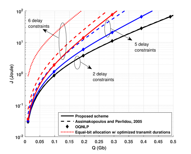
Figure 1: Total transmission energy $J$ from our scheme, that by [13], and the optimum by OQNLP are shown with total average bits $Q$.

In Fig. 2, we show the data rates resulting from our bit-allocation scheme for all 5 data sets or users ($k=1,2,\ldots,5$). In the first trial, we set the maximum delay of all sets $T_{k}=4$ s and total bits for each set to be $0.17Q$, $0.05Q$, $0.10Q$, $0.48Q$, and $0.20Q$, respectively where $Q=500$ Mb. We see that the resulting data rates for all sets are equal to 125 Mbps. Since the delay constraints in this trial are not too limiting, our scheme produces the solution with equal rates as discussed in Section 3. We compare with the data rates obtained from [13] and see that data rate for each user is not the same. The data rate from [13] is simply obtained by dividing the total bits for a user by the maximum delay. Thus, user 4 with the largest number of bits to transmit has the maximum data rate. We also display the total transmit energy for both schemes and see that our scheme consumes close to half of what [13] does. The results from the second trial with different maximum delay and set of total bits are also shown with dashed lines. The same observation for the first trial can also been made.

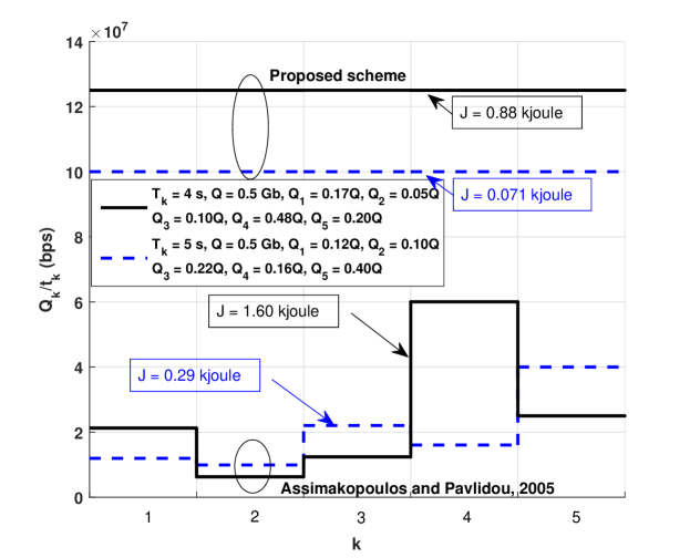
Figure 2: Data rates for all sets/users from the proposed scheme are compared with those from the scheme by [13].

In Fig 3, we examine the number of active subchannels as data rate increases. For our proposed allocation, the number of active subchannels for data set $k$ depends on the threshold $\lambda_{k}$ and rate $Q_{k}/t_{k}$ as shown in (31). The dash-dot curve is obtained from solving $\lambda_{k}$ in (31) for the given rate and then using (32) to find the number of active subchannels. For the other plots from the proposed scheme, we set $K=3$ with $T_{k}=0.25$, $1$, and $5$ s and $Q_{k}=0.25Q$, $0.2Q$, and $0.55Q$ with increasing $Q$. The number of active subchannels for all three data sets is displayed with different markers and are shown to be on the dash-dot curve as expected. We also show the number of active subchannels obtained from the allocation scheme by [13] with $T_{k}=5$ s, $\forall k$. We see that with [13], the number of active subchannels for a different data set does not follow the dash-dot curve. In [13], allocating the number of subchannels for each set will depend on the rates of all sets as well as subchannel quality. Since user 3 ($k=3$) has the largest rate requirement of all three users, the user is allocated the most number of active subchannels.

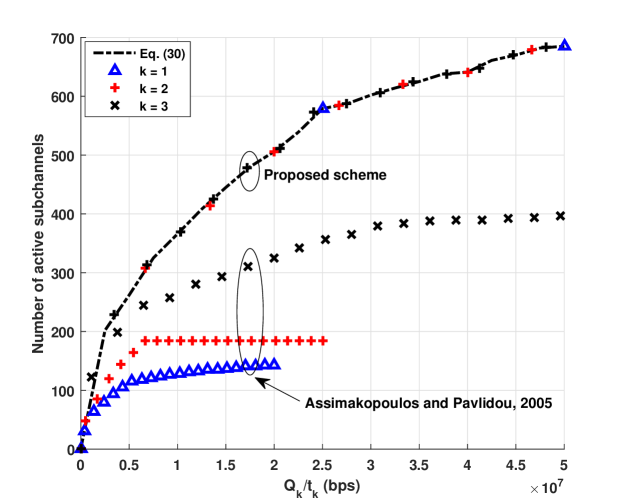
Figure 3: The number of active subchannels is shown with data rate for $K=3$.

In Fig. 4, we show the total energy obtained from the proposed allocation for systems with $K=5$, $T_{k}=0.625$, $1.25$, $1.875$, $3.125$, and $5$ s, and the following set of total bits $\{0.25Q,0.10Q,0.20Q,0.25Q,0.10Q\}$. We see that the total transmit energy must increase with the sum of total bits for all data sets denoted by $Q$. We also consider the ideal channels with no impulsive noise or narrowband interference. It is not surprising that the total transmit energy is reduced with the ideal channels. However, we note that energy reduction is small when the number of total bits $Q$ is small and is increasing with $Q$. Thus, impulsive noise and narrowband interference have a larger impact when large number of bits needs to be transmitted. We also vary the quality of the channel or CNR by increasing or decreasing the channel power of all subchannels by 5 or 10 dB and observe that the energy difference is large when the average CNR is increased or decreased significantly.

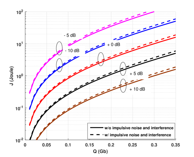
Figure 4: Total transmission energy of the proposed allocation for systems with impulsive noise and narrowband interference as indicated in Table 1 is compared with that of the ideal systems without impulsive noise and interference.

5 Conclusions

From the study, we find that the optimal bit allocation over subchannels, the optimal transmit duration, and the number of active subchannels, depend largely on the transmission rate of each data set and quality of subchannels, which is indicated by CNR and the probability of narrowband interference and impulsive noise. Our proposed bit allocation is optimal with 2 delay constraints and performs close to the optimum with more than 2 delay constraints. It is also less complex than solving for the optimal allocation. From numerical results, our scheme is shown to outperform the allocation scheme by [13] especially with large amount of data and larger number of delay constraints. Systems with narrowband interference and impulsive noise require higher transmission energy. Furthermore, the energy increase over that of systems with no or very small probability of impulsive noise is more pronounced with large total-bit requirements. Besides PLC, the proposed bit allocation can be applied to other applicable OFDM channels such as wireless multipath channels or wired transmission over twisted-pair cables with narrowband interference.

References

References

- [1] Broadband over power line networks: Medium access control and physical layer specifications, Standard IEEE 1901-2010, IEEE (2010).
- [2] M. Zimmermann, K. Dostert, A multipath model for the powerline channel, IEEE Trans. Commun. 50 (4) (2002) 553–559.
- [3] S. P. Herath, N. H. Tran, T. Le-Ngoc, On optimal input distribution and capacity limit of Bernoulli-Gaussian impulsive noise channels, in: Proc. IEEE International Conference on Communications (ICC), Ottawa, ON, Canada, 2012, pp. 3429–3433.
- [4] M. Zimmermann, K. Dostert, Analysis and modeling of impulsive noise in broad-band powerline communications, IEEE Trans. Electromagn. Compat. 44 (1) (2002) 249–258. doi:10.1109/15.990732.
- [5] T. Shongwe, V. N. Papilaya, A. J. H. Vinck, Narrow-band interference model for OFDM systems for powerline communications, in: Proc. IEEE Int. Symp. on Power Line Commun. and Its Applications Conf. (ISPLC), Johannesburg, South Africa, 2013, pp. 268–272.
- [6] Z. Shen, J. G. Andrews, B. L. Evans, Adaptive resource allocation in multiuser OFDM systems with proportional rate constraints, IEEE Trans. Wireless Commun. 4 (6) (2005) 2726–2737.
- [7] K. Liu, B. Tang, Y. Liu, Adaptive power loading based on unequal-BER strategy for OFDM systems, IEEE Commun. Lett. 13 (7) (2009) 474–476.
- [8] A. Chaudhuri, M. R. Bhatnagar, Optimised resource allocation under impulsive noise in power line communications, IET Commun. 8 (7) (2014) 1104–1108.
- [9] J. Shin, J. Jeong, Improved outage probability of indoor PLC system for multiple users using resource allocation algorithms, IEEE Trans. Power Del. 28 (4) (2013) 2228–2235.
- [10] A. Hamini, J.-Y. Baudais, J.-F. Hélard, Green resource allocation for powerline communications, in: Proc. IEEE Int. Symp. on Power Line Commun. and Its Applications Conf. (ISPLC), Udine, Italy, 2011, pp. 393–398.
- [11] F. Pancaldi, F. Gianaroli, G. M. Vitetta, Bit and power loading for narrowband indoor powerline communications, IEEE Trans. Commun. 64 (7) (2016) 3052–3063. doi:10.1109/TCOMM.2016.2575838.
- [12] P. Kas-udom, W. Santipach, Minimum-energy bit allocation over powerline OFDM channels, in: Proc. Int. Conf. on Electrical Engineering/Electronics, Computer, Telecommun. and Info. Technol. (ECTI-CON), Krabi, Thailand, 2013, pp. 1–5. doi:10.1109/ECTICon.2013.6559604.
- [13] C. Assimakopoulos, F.-N. Pavlidou, Multiuser power and bit allocation over power line channels, in: Proc. IEEE Int. Symp. on Power Line Commun. and Its Applications Conf. (ISPLC), Vancouver, Canada, 2005, pp. 255–259.
- [14] R. K. Sundaram, A First Course in Optimization Theory, Cambridge University Press, 1996, Ch. Inequality Constraints and the Theorem of Kuhn and Tucker, pp. 145–171.
- [15] R. L. Burden, J. D. Faires, Numerical Analysis, 9th Edition, Brooks/Cole, Boston, MA, USA, 2011, Ch. 2.1 The Bisection Algorithm, pp. 48–54.
- [16] L. D. Bert, P. Caldera, D. Schwingshack, A. M. Tonello, On noise modeling for power line communications, in: Proc. IEEE Int. Symp. on Power Line Commun. and Its Applications Conf. (ISPLC), Udine, Italy, 2011, pp. 283–288.