Tidal disruption flares from stars on marginally bound and unbound orbits

Abstract

We study the mass fallback rate of tidally disrupted stars on marginally bound and unbound orbits around a supermassive black hole (SMBH) by performing three-dimensional smoothed particle hydrodynamic (SPH) simulations with three key parameters. The star is modeled by a polytrope with two different indexes ($n=1.5$ and $3$). The stellar orbital properties are characterized by five orbital eccentricities ranging from $e=0.98$ to $1.02$ and five different penetration factors ranging from $\beta=1$ to $3$, where $\beta$ represents the ratio of the tidal disruption to pericenter distance radii. We derive analytic formulae for the mass fallback rate as a function of the stellar density profile, orbital eccentricity, and penetration factor. Moreover, two critical eccentricities to classify tidal disruption events (TDEs) into five different types: eccentric ($e<e_{\rm crit,1}$), marginally eccentric ($e_{\rm crit,1}\lesssim{e}<1$), purely parabolic ($e=1$), marginally hyperbolic ($1<e<e_{\rm crit,2}$), and hyperbolic ($e\gtrsim{e_{\rm crit,2}}$) TDEs, are reevaluated as $e_{\rm crit,1}=1-2q^{-1/3}\beta^{k-1}$ and $e_{\rm crit,2}=1+2q^{-1/3}\beta^{k-1}$, where $q$ is the ratio of the SMBH to stellar masses and $0<k\lesssim 2$. We find the asymptotic slope of the mass fallback rate varies with the TDE type. The asymptotic slope approaches $-5/3$ for the parabolic TDEs, is steeper for the marginally eccentric TDEs, and is flatter for the marginally hyperbolic TDEs. For the marginally eccentric TDEs, the peak of mass fallback rates can be about one order of magnitude larger than the parabolic TDE case. For marginally hyperbolic TDEs, the mass fallback rates can be much lower than the Eddington accretion rate, which can lead to the formation of a radiatively inefficient accretion flow, while hyperbolic TDEs lead to failed TDEs. Marginally unbound TDEs could be an origin of a very low density gas disk around a dormant SMBH.

1 Introduction

There is growing evidence that supermassive black holes (SMBHs) ubiquitously reside at the center of galaxies, based on observations of stellar proper motion, stellar velocity dispersion or accretion luminosity (Kormendy & Ho, 2013). Tidal disruption events (TDEs) provide a distinct opportunity to probe dormant SMBHs in inactive galaxies. Once a star approaches a SMBH and enters inside the tidal sphere, the star is tidally disrupted by the SMBH. The stellar debris then falls back to the SMBH at a super-Eddington rate, leading to a prominent flaring event with a luminosity exceeding the Eddington luminosity for weeks to months (Rees, 1988; Phinney, 1989; Evans & Kochanek, 1989).

Tidal disruption flares have been observed over the broad range of waveband from optical (van Velzen et al. 2011; Gezari et al. 2012; Holoien et al. 2016) to ultraviolet (Gezari et al., 2006, 2008; Chornock et al., 2014) to soft X-ray (Komossa & Bade 1999; Saxton et al. 2012; Maksym et al. 2013; Auchettl et al. 2017) wavelengths. The TDE rates have been estimated to be $10^{-5}-10^{-4}$ per year per galaxy for soft-X-ray selected TDEs (Donley et al., 2002; Esquej et al., 2008) and for optical-selected TDEs (van Velzen & Farrar, 2014; Holoien et al., 2016; van Velzen, 2018; Hung et al., 2018). The observed rates are consistent with the theoretically expected rates (Wang & Merritt 2004; Stone & Metzger 2016; see also Komossa 2015 and Stone et al. 2020 for a recent review). On the other hand, high-energy jetted TDEs have been detected through non-thermal emissions at radio (Zauderer et al., 2011; Alexander et al., 2016; van Velzen et al., 2016) and/or hard X-ray (Burrows et al., 2011; Brown et al., 2015) wavelengths with much lower event rate than the thermal TDE case (Farrar & Piran, 2014). Spectroscopic studies have confirmed ${\rm H\,I}$ and ${\rm He\,II}$ (Arcavi et al. 2014) as well as metal lines (Leloudas et al. 2019). Recently discovered blue-shifted (0.05c) broad absorption lines are likely to result from a high velocity outflow produced by the candidate TDE AT2018zr (Hung et al. 2019).

It still remains under debate how the standard, theoretical mass fallback rate, which is proportional to $t^{-5/3}$ (Rees, 1988; Phinney, 1989; Evans & Kochanek, 1989), can be translated into the observed light curves. Dozens of X-ray TDEs have light curves shallower than $t^{-5/3}$ (Auchettl et al., 2017), while many optical/UV TDEs are well fit by $t^{-5/3}$ (e.g. Hung et al. 2017) but some deviate from $t^{-5/3}$ (Gezari et al., 2012; Chornock et al., 2014; Arcavi et al., 2014; Holoien et al., 2014). Specifically, the slope of the light curve depends on when measurements are taken relative to the peak. PS1-10JH shows a light curve more consistent with $t^{-5/3}$ at late times as shown by Gezari et al. (2015). The decay rate becomes flatter at very late times (van Velzen et al., 2019). This flattening likely reflects the evolution of a viscously spreading disk rather than the continued evolution of the mass fallback rate (Cannizzo et al., 1990; Cannizzo & Gehrels, 2009; Shen & Matzner, 2014).

There have been some arguments that the mass fallback rate itself can deviate from the $t^{-5/3}$ decay rate. Lodato et al. (2009) demonstrated that the stellar internal structure makes the mass fallback rate deviate from the standard fallback rate in an early time. When the star is simply modeled by a polytrope, the stellar density profile is characterized by a polytropic index. In this case, the polytrope index is a key parameter to determine the mass fallback rate.

The penetration factor, which is the ratio of the tidal disruption to pericenter radii, is also an important parameter for TDEs. Guillochon & Ramirez-Ruiz (2013) showed that resultant light curves can be steeper because of the centrally condensed core surviving after the partial disruption of the star. It would happen if the penetration factor is relatively low ($\beta\lesssim 2$ for the case that the polytropic index equals to 3) (Mainetti et al., 2017). The self-gravity of the survived core can change the trajectories of the striped material and therefore the resultant mass fallback rate as well (MacLeod et al., 2012). The penetration factor also plays an important role in the process of debris circularization. The energy dissipation of a strong shock by a collision between the debris head and tail naturally leads to the formation of an accretion disk (Hayasaki et al., 2013; Bonnerot et al., 2016; Hayasaki et al., 2016), although the detailed dissipation mechanism is still under debate (Stone et al., 2013; Shiokawa et al., 2015; Piran et al., 2015). Moreover, the penetration factor is a key parameter to determine the size and temperature of the circularized accretion disk (Dai et al., 2015). Recent X-ray observation suggests that the TDE would happen with very high penetration factor (Pasham et al., 2018).

In the case of tidal disruption of a star on an elliptical orbit, Hayasaki et al. (2013) found that the resultant mass fallback rate is higher with smaller orbital eccentricity because the fallback timescale is much shorter and more material is bound to the SMBH compared to the parabolic orbit case. In contrast, the mass fallback rate can be much smaller than the Eddington rate or even zero for a hyperbolic orbit case. Hayasaki et al. (2018) proposed that there are two critical eccentricities to classify TDEs into five different types by the stellar orbit: eccentric ($e<e_{\rm crit,1}$), marginally eccentric ($e_{\rm crit,1}\lesssim{e}<1$), purely parabolic ($e=1$), marginally hyperbolic ($1<e<e_{\rm crit,2}$), and hyperbolic ($e\gtrsim{e_{\rm crit,2}}$) TDEs, respectively, where $e_{\rm crit,1}=1-2q^{-1/3}\beta^{-1}$ and $e_{\rm crit,2}=1+2q^{-1/3}\beta^{-1}$, and $q$ is the ratio of the SMBH to stellar masses. Based on this classification, they also examined the frequency of each TDE by N-body experiments. They pointed out that stars on marginally elliptical and hyperbolic orbits can be a main TDE source in a spherical star cluster. Therefore, it is clear that the orbital eccentricity (and semi-major axis through the penetration factor) is also a key parameter to make the mass fallback rate deviate from the standard $t^{-5/3}$ decay rate.

However, there is still little known about how the three key parameters: polytropic index, penetration factor, and orbital eccentricity, and their combinations affect the mass fallback rate. In this paper, we therefore revisit the mass fallback rate onto an SMBH or IMBH by taking account of the three key parameters. In Section 2, we give a new condition to classify the TDEs by the stellar orbital type based on the assumption that the spread in debris energy is proportional to the $k$-th power of the penetration factor, where $k$ is presumed to range for $0<k<2$ (see Stone et al. 2013). In addition, we derive analytically the formula of the mass fallback rates, which includes the effect of the three key parameters plus $k$ on them. In Section 3, we describe our numerical simulation approach and compare the semi-analytical solutions of the mass fallback rates with the simulation results. Finally, Section 4 is devoted to the conclusion of our scenario.

2 Revisit of mass fallback rates

In this section, we revisit the mass fallback rate by taking account of a stellar density profile (Lodato et al., 2009) and the orbital eccentricity (Hayasaki et al., 2018), including the dependence of the penetration factor, $\beta=r_{\rm t}/r_{\rm p}$, where $r_{\rm p}$ is the pericenter distance, on a spread in debris specific energy. As a star approaches to a SMBH or an IMBH, it is torn apart by the tidal force of the black hole, which dominates the self-gravity of the star at the tidal disruption radius:

$$r_{\rm t}=\left(\frac{M_{\rm bh}}{m_{*}}\right)^{1/3}r_{*}\approx 24\left(\frac{M_{\rm bh}}{10^{6}\,{M}_{\odot}}\right)^{-2/3}\left(\frac{m_{*}}{{M}_{\odot}}\right)^{-1/3}\left(\frac{r_{*}}{{R}_{\odot}}\right)r_{\rm S}.$$ (1)

Here we denote the black hole mass as $M_{\rm bh}$, stellar mass and radius as $m_{*}$ and $r_{*}$, and the Schwarzschild radius as $r_{\rm S}=2{\rm G}M_{\rm bh}/{\rm c}^{2}$, where $G$ and $c$ are Newton’s gravitational constant and the speed of light, respectively.

Following Stone et al. (2013), the tidal force produces a spread in specific energy of the stellar debris:

$$\Delta\mathcal{E}=\beta^{k}\Delta\epsilon,$$ (2)

where $k$ is the power-law index of the penetration factor in the leading order term of the tidal potential energy (hereafter, tidal spread energy index) and

$$\Delta\epsilon=\frac{GM_{\rm bh}r_{*}}{r_{\rm t}^{2}}$$ (3)

is the standard spread energy (Rees, 1988; Evans & Kochanek, 1989). If $\beta=1$ or $k=0$, Equation (2) reduces to the standard equation. The possible range of $k$ has been taken as $0\leq{k}\leq 2$.

The mass fallback rate can be written by the chain rule as

$$\frac{dM}{dt}=\frac{dM}{d\epsilon}\frac{d\epsilon}{dt},$$ (4)

where $dM/d\epsilon$ is the differential mass distribution of the stellar debris with specific energy $\epsilon$. Because the thermal energy of the stellar debris is negligible compared with the debris binding energy, $\epsilon\approx\epsilon_{\rm d}$:

$$\epsilon_{\rm d}\equiv-\frac{GM_{\rm bh}}{2a_{\rm d}},$$ (5)

where $a_{\rm d}$ is the semi-major axis of the stellar debris. Applying the Kepler’s third law to equation (5), we obtain that

$$\frac{d\epsilon_{\rm d}}{dt}=\frac{1}{3}(2\pi{GM}_{\rm bh})^{2/3}t^{-5/3}.$$ (6)

2.1 Effect of stellar density profiles

Lodato et al. (2009) included the effect of the stellar density profile on the differential mass distribution of the stellar debris as

$$\frac{dM}{d\epsilon_{\rm d}}=\frac{dM}{d\Delta r}\frac{d\Delta r}{d\epsilon_{\rm d}},$$ (7)

where $\Delta r$ is the radial width of the star. In our case, the relation between the radial width and the debris specific binding energy is given by

$$\frac{\Delta r}{r_{*}}=\frac{|\epsilon_{\rm d}|}{\Delta\mathcal{E}}=\frac{\mathcal{A}_{c}}{a_{\rm d}},$$ (8)

where $\mathcal{A}_{\rm c}$ is the critical semi-major axis:

$$\mathcal{A}_{\rm c}=a_{\rm c}\beta^{-k},$$ (9)

with $a_{\rm c}\equiv(M_{\rm bh}/m_{*})^{1/3}r_{\rm t}/2$. If $\beta=1$ or $k=0$ is adopted here, equation (8) reduces to that of Lodato et al. (2009). Moreover, the radial width depends on the orbital period of the stellar debris through the binding energy, i.e., $\Delta{r}\propto{a}_{\rm d}^{-1}\propto{t^{-2/3}}$.

The internal density structure of the star is given by the radial integral of the stellar density

$$\frac{dM}{d\Delta r}=2\pi\int_{\Delta r}^{r_{*}}\rho\left(r\right)r{\rm d}r,$$ (10)

where $\rho\left(r\right)$ is the spherically symmetric mass density of the star and the polytropes with no stellar rotation are considered. We can integrate equation (10) by solving the Lane-Emden equation: $\left(1/\xi^{2}\right)d\left(\xi^{2}d\theta/d\xi\right)/d\xi=-\theta^{n}$, where $\theta\left(\xi\right)=\rho/\rho_{\rm c}$, $\xi=r/r_{\rm c}$, $\rho_{\rm c}$ is the normalization density, $r_{\rm c}=\sqrt{(n+1)K\rho_{\rm c}^{1/n-1}/4\pi{G}}$ is the normalization radius, $n$ is a polytropic index, $K$ is a polytropic constant, respectively (Chandrasekhar, 1967). Substituting equations (8) and (10) into equation (7), we obtain the differential mass distribution as

$$\frac{dM}{d\epsilon_{\rm d}}=\frac{3}{2}\left(\frac{\rho_{\rm c}}{\bar{\rho}}\right)\left(\frac{r_{\rm c}}{r_{*}}\right)^{2}\left(\frac{m_{*}}{\Delta\mathcal{E}}\right)\int_{\Delta{r}/r_{\rm c}}^{r_{*}/r_{\rm c}}\theta\left(\xi\right)\xi{\rm d}\xi,$$ (11)

where $\bar{\rho}=m_{*}/(4\pi{r_{*}^{3}}/3)$ is the mean density of the star. Because $\theta(\xi)$ is obtained by solving the Lane-Emden equation numerically, $dM/d\epsilon_{\rm d}$ is semi-analytically determined (see also Figure 2). Following the Kepler’s third law, we can estimate the orbital period of the most tightly bound debris as

$$t_{\rm mtb}^{{}^{\prime}}=2\pi\sqrt{\frac{\mathcal{A}_{\rm c}^{3}}{GM_{\rm bh}}}=t_{\rm mtb}\beta^{-3k/2},$$ (12)

where $t_{\rm mtb}=2\pi\sqrt{a_{c}^{3}/GM_{\rm bh}}$ corresponds to the $\beta=1$ case. Substituting equations (6) and (11) into equation (4), we obtain the mass fallback rate:

$$\frac{dM}{dt} = \left(\frac{\rho_{\rm c}}{\bar{\rho}}\right)\left(\frac{r_{\rm c}}{r_{*}}\right)^{2}\left(\frac{m_{*}}{t_{\rm mtb}^{{}^{\prime}}}\right)\left(\frac{t}{t_{\rm mtb}^{{}^{\prime}}}\right)^{-5/3}\int_{\Delta{r}/r_{\rm c}}^{r_{*}/r_{\rm c}}\theta\left(\xi\right)\xi{\rm d}\xi$$ (13)

$$= \left(\frac{\rho_{\rm c}}{\bar{\rho}}\right)\left(\frac{r_{\rm c}}{r_{*}}\right)^{2}\left(\frac{1}{\beta^{k}}\right)\left(\frac{m_{*}}{t_{\rm mtb}}\right)\left(\frac{t}{t_{\rm mtb}}\right)^{-5/3}\int_{\Delta r/r_{\rm c}}^{r_{*}/r_{\rm c}}\theta(\xi)\xi d\xi$$

For $n=3$ and $\xi\ll 1$, the normalized density can be expanded to be $\theta(\xi)\approx 1-\xi^{2}/6+\mathcal{O}(\xi^{4})$. Since we obtain from equation (8) and (12) that $\Delta{r}/r_{\rm c}=(r_{*}/r_{\rm c})(t/t_{\rm mtb})^{-2/3}\beta^{-k}$, we can approximately estimate the mass fallback rate as $dM/dt\approx(1/2)(\rho_{c}/\bar{\rho})(1/\beta^{k})(m_{*}/t_{\rm mtb})(t/t_{\rm mtb})^{-5/3}[1-(t/t_{\rm mtb})^{-4/3}\beta^{-2k}][1-(1/12)(r_{*}/r_{\rm c})^{2}(1+(t/t_{\rm mtb})^{-4/3}\beta^{-2k})]$. We find that the mass fallback rate depends on not only the stellar density profile but also the penetration factor and the tidal spread energy index, which leads to the deviation from $t^{-5/3}$.

2.2 Effect of stellar orbital properties

In this section, we investigate stars that approach the SMBH on parabolic, eccentric, and hyperbolic orbits. The specific energy of the stellar debris is in the range of $-\Delta\mathcal{E}-GM/(2a)\leq{\epsilon_{\rm d}}\leq\Delta\mathcal{E}+GM/(2a)$, where $a$ is the orbital semi-major axis of the approaching star.

Following Hayasaki et al. (2018), the TDEs are classified by the critical eccentricities in terms of the orbital eccentricity of the star:

$$\left\{\begin{array}[]{ll}0\leq e<e_{\rm crit,1}&{\rm eccentric\,\,TDEs}\\ e_{\rm crit,1}\leq e<1&{\rm marginally\,\,eccentric\,\,TDEs}\\ e=1&{\rm parabolic\,\,TDEs}\\ 1<e\leq e_{\rm crit,2}&{\rm marginally\,\,hyperbolic\,\,TDEs}\\ e_{\rm crit,2}<e&{\rm hyperbolic\,\,TDEs},\\ \end{array}\right.$$ (19)

where $e_{\rm crit,1}$ and $e_{\rm crit,2}$ are modified as

$$e_{\rm crit,1} = 1-2q^{-1/3}\beta^{k-1},$$

$$e_{\rm crit,2} = 1+2q^{-1/3}\beta^{k-1}$$ (20)

with $q\equiv{M}_{\rm bh}/m_{*}$, respectively. If $\beta=1$ or $k=0$, these two terms reduce to the previously defined critical eccentricities (see equations (5) and (6) of Hayasaki et al. 2018). The modified specific binding energy of the most tightly bound stellar debris for eccentric or hyperbolic stellar orbits is given by

$$\epsilon_{\rm mtb}=-\Delta\mathcal{E}\pm\frac{GM_{\rm bh}}{2a}=-\left(1\mp\frac{\mathcal{A}_{\rm c}}{a}\right)\Delta\mathcal{E},$$ (21)

where the negative and positive signs of the specific orbital energy of the star indicate the eccentric and hyperbolic orbit cases, respectively. The orbital period of the most tightly bound debris is also changed as

$$\tau_{\rm mtb}=2\pi\sqrt{\frac{\mathcal{A}_{\rm c}^{3}}{GM_{\rm bh}}}\left(1\mp\frac{\mathcal{A}_{\rm c}}{a}\right)^{-3/2}=t_{\rm mtb}\left(\beta^{-3k/2}\right)\left(1\mp\frac{\mathcal{A}_{\rm c}}{a}\right)^{-3/2},$$ (22)

where we use equation (12) and $\mathcal{A}_{\rm c}/a$ should be smaller than unity for the upper negative sign (hyperbolic TDE) case. The differential mass distribution is thus changed from equation (11) to

$$\frac{dM}{d\epsilon_{\rm d}}=\frac{3}{2}\left(\frac{\rho_{\rm c}}{\bar{\rho}}\right)\left(\frac{r_{\rm c}}{r_{*}}\right)^{2}\left(\frac{m_{*}}{\Delta\mathcal{E}}\right)\int_{\Delta{r}^{{}^{\prime}}/r_{\rm c}}^{r_{*}/r_{\rm c}}\theta\left(\xi\right)\xi{\rm d}\xi,$$ (23)

where $\Delta{r}^{{}^{\prime}}$ is the newly defined radial width of the star and is given by

$$\frac{\Delta{r}^{{}^{\prime}}}{r_{*}}=\frac{|\epsilon_{\rm d}^{{}^{\prime}}|}{\Delta\mathcal{E}}=\frac{\mathcal{A}_{\rm c}}{a_{\rm d}}\left(1\mp\frac{a_{\rm d}}{a}\right)$$ (24)

with the modification of the debris binding energy, i.e., $\epsilon_{\rm d}^{{}^{\prime}}=-GM/(2a_{\rm d})\pm{GM}/(2a)$. Note that $\theta(\xi)=0$ if $\Delta{r}^{{}^{\prime}}/r_{*}$ is greater than unity because there is no stellar gas there.

Substituting equations (6) and (23) into equation (4) and applying equations (21) and (22), we can obtain the modified mass fallback rate as

$$\frac{dM}{dt} =\left(\frac{\rho_{\rm c}}{\bar{\rho}}\right)\left(\frac{r_{\rm c}}{r_{*}}\right)^{2}\left(1\mp\frac{\mathcal{A}_{\rm c}}{a}\right)\left(\frac{m_{*}}{\tau_{\rm mtb}}\right)\left(\frac{t}{\tau_{\rm mtb}}\right)^{-5/3}\int_{\Delta{r}^{{}^{\prime}}/r_{\rm c}}^{r_{*}/r_{\rm c}}\theta\left(\xi\right)\xi{\rm d}\xi.$$

$$=\left(\frac{\rho_{\rm c}}{\bar{\rho}}\right)\left(\frac{r_{\rm c}}{r_{*}}\right)^{2}\left(\frac{1}{\beta^{k}}\right)\left(\frac{m_{*}}{t_{\rm mtb}}\right)\left(\frac{t}{t_{\rm mtb}}\right)^{-5/3}\int_{\Delta{r}^{{}^{\prime}}/r_{\rm c}}^{r_{*}/r_{\rm c}}\theta\left(\xi\right)\xi{\rm d}\xi.$$ (25)

Applying $\theta(\xi)\simeq 1-\xi^{2}/6+O(\xi^{4})$ to equation (25) for the $n=3$ and $\xi\ll 1$ case, we approximately estimate the mass fallback rate as $dM/dt\approx(\rho_{c}/\bar{\rho})(1/\beta^{k})(m_{*}/t_{\rm mtb})(t/t_{\rm mtb})^{-5/3}[1-(t/t_{\rm mtb})^{-4/3}\beta^{-2k}[1+(t/t_{\rm mtb})^{2/3}(a_{\rm c}/a)]^{2}][1-(1/12)(r_{*}/r_{\rm c})^{2}(1+(t/t_{\rm mtb})^{-4/3}\beta^{-2k}[1+(t/t_{\rm mtb})^{2/3}(a_{\rm c}/a)]^{2})]$. This is applied only for eccentric to parabolic orbit cases and is not valid for the hyperbolic orbit case, because the expansion formula of $\theta(\xi)$ corresponds to the density profile of the central part of the approaching star, which is unbound to the black hole if the star is on a hyperbolic orbit. We find the mass fallback rate depends on the stellar density profile with the orbital eccentricity (or semi-major axis), the penetration factor, and the tidal spread energy index, leading to the deviation from $t^{-5/3}$. We test this hypothesis by numerical simulations and describe our results in Section 3.

2.3 Numerical simulations

We evaluate how well the analytical solution matches the numerical simulations by using a three-dimensional (3D) Smoothed Particle Hydrodynamics (SPH) code. The SPH code is developed based on the original version of Benz (1990); Benz et al. (1990) and substantially modified as described in Bate et al. (1995) and parallelized using both OpenMP and MPI.

Two-stage simulations are performed to model a tidal interaction between a star and a black hole. In the first-stage simulation, we model the star by a polytrope with $n=1.5$ and $n=3$ for a solar-type star. We run the simulations until the polytrope is virialized. In the second-stage simulation, the star is initially located at a distance of three times the tidal disruption radii and approaches the SMBH following Kepler’s third law for five orbital eccentricities and five different penetration factors per each orbital eccentricity. In summary, we run a total 50 simulations in the second-stage. The stellar mass, stellar radius, and black hole mass are held constant throughout the simulations at $m_{*}=1\,M_{\odot}$, $r_{*}=1\,R_{\odot}$, and $M_{\rm{bh}}=10^{6}\,M_{\odot}$, respectively. The total number of SPH particles used in each simulation is slightly more than $10^{6}$ and the run time is measured in units of $\Omega_{*}^{-1}=\sqrt{r_{*}^{3}/(Gm_{*})}\simeq 1.6\times 10^{3}\,\rm{s}$.

Tables 1 and 2 present a summary of the SPH simulation models and the corresponding spread energy indices obtained from the simulations. For both tables, the first to third columns show the polytropic index ($n$), the penetration factor ($\beta$), and the orbital eccentricity ($e$), respectively. The fourth and fifth columns show two critical eccentricities $e_{\rm crit,1}$ and $e_{\rm crit,2}$, respectively (see equation 20). The final column presents the tidal spread energy index ($k$), which is estimated by fitting the simulation data (see the detail in Section 3.2). We find from Tables 1 and 2 that the $e=0.98$ and $e=0.99$, $e=1.0$, $e=1.01$, and $e=1.02$ cases correspond to marginally eccentric, parabolic, marginally hyperbolic, hyperbolic TDEs, respectively.

Table 1: Summary for parameters of our simulations. The first column shows the polytrope index ($n$). The second and third columns present the penetration factor ($\beta$) and the orbital eccentricity ($e$), respectively. The fourth and fifth columns show the two critical eccentricities $e_{\rm crit,1}$ and $e_{\rm crit,2}$, respectively (see equation 20). The final column presents the specific energy index ($k$), which is obtained by fitting the simulation data (see equation 26.

$n$	$\beta$	$e$	$e_{\rm crit,1}$	$e_{\rm crit,2}$	$k$
	1		0.980	1.02	$-$
	1.5		0.983	1.02	0.595
1.5	2	0.98	0.987	1.01	0.332
	2.5		0.989	1.01	0.293
	3		0.982	1.02	0.902
	1		0.980	1.02	$-$
	1.5		0.983	1.02	0.593
1.5	2	0.99	0.987	1.00	0.327
	2.5		0.989	1.01	0.287
	3		0.982	1.02	0.897
	1		0.980	1.02	$-$
	1.5		0.983	1.02	0.646
1.5	2	1.0	0.987	1.01	0.324
	2.5		0.989	1.01	0.273
	3		0.990	1.01	0.323

$n$	$\beta$	$e$	$e_{\rm crit,1}$	$e_{\rm crit,2}$	$k$
	1		0.980	1.02	$-$
	1.5		0.983	1.02	0.584
1.5	2	1.01	0.988	1.01	0.317
	2.5		0.989	1.01	0.275
	3		0.991	1.01	0.318
	1		0.980	1.02	$-$
	1.5		0.983	1.02	0.580
1.5	2	1.02	0.988	1.01	0.312
	2.5		0.989	1.01	0.270
	3		0.991	1.01	0.313

Table 2: Summary for parameters of our simulations. The format of each column is the same as Table 1, but for the $n=3$ case.

$n$	$\beta$	$e$	$e_{\rm crit,1}$	$e_{\rm crit,2}$	k
	1		0.980	1.02	$-$
	1.5		0.968	1.03	2.17
3	2	0.98	0.970	1.03	1.58
	2.5		0.976	1.02	1.19
	3		0.980	1.02	00.981
	1		0.980	1.02	$-$
	1.5		0.968	1.03	2.14
3	2	0.99	0.970	1.03	1.57
	2.5		0.976	1.02	1.19
	3		0.980	1.02	00.978
	1		0.980	1.02	$-$
	1.5		0.968	1.03	2.12
3	2	1.0	0.970	1.03	1.57
	2.5		0.976	1.02	1.19
	3		0.981	1.02	00.974

$n$	$\beta$	$e$	$e_{\rm crit,1}$	$e_{\rm crit,2}$	$k$
	1		0.980	1.02	$-$
	1.5		0.969	1.03	2.10
3	2	1.01	0.971	1.03	1.56
	2.5		0.976	1.02	1.19
	3		0.981	1.02	00.971
	1		0.980	1.02	$-$
	1.5		0.969	1.03	2.07
3	2	1.02	0.971	1.03	1.55
	2.5		0.976	1.02	1.18
	3		0.981	1.02	00.967

3 Results

In this section, we describe the simulation results in order to compare our semi-analytical prediction with that of the SPH simulations.

3.1 Differential mass distribution of stellar debris

We first compare the simulated differential mass distribution of the stellar debris over the specific energy measured at a run time of $t=4$ with the Gaussian-fitted distributions; we then compare our findings with the semi-analytical solution given by equation (25). The relevance of the fitting is also discussed.

Figure 1 shows the energy distribution of the debris for $n=1.5$ with five different penetration factors. Panel (a) shows the differential mass distribution for the standard, parabolic case ($e=1.0$). Panels (b)-(e) show results for the marginally eccentric ($e=0.98$ and $0.99$) and marginally hyperbolic ($e=1.01$ and $e=1.02$) TDE cases, respectively. In all the panels, the red, green, blue, magenta, and brown color points are the differential mass distributions for $\beta=1$, $\beta=1.5$, $\beta=2$, $\beta=2.5$, and $\beta=3$, respectively. The corresponding fitted curves are obtained using the FindFit model provided by Mathematica and are represented in the same color format. It can find a non-linear fitting with the gaussian function, $f(x)=(1/\sqrt{2\pi}\sigma)\exp[-(1/2)([x-\mu]/\sigma)^{2}]$, where $\mu$ is the position of the center of the peak and $\sigma$ is the standard deviation which is proportional to a half width at half maximum (HWHM). We also simply evaluate the accuracy of the fitting by using the root mean square (RMS) and its square is given by ${\rm RMS}^{2}\,=\sum_{i=1}^{N_{\rm d}}\,([y_{i}-f(x_{i})]/f(x_{i}))^{2}/N_{\rm d}$, where $N_{\rm d}$ is the number of data points, and $x_{i}$ and $y_{i}$ are the normalized specific energy at the $i$-th data point and the corresponding differential mass distribution, respectively. We evaluate the RMS using only points within $1\,\sigma$ of the Gaussian fitted curve, $\Delta\mathcal{E}_{\rm sim}$. We confirm that for parabolic TDEs, the differential mass is distributed around a specific energy of zero and also a half of the debris mass, independently of $\beta$, is bound by the SMBH. As we predicted in Section 2.2, the position of the peak of the differential mass is shifted in the negative direction for eccentric TDEs and the resultant differential mass is distributed over there, while the position of the peak is positively shifted for the hyperbolic TDE cases. The deviation of the peak position corresponds to $a_{\rm c}/a$ to an accuracy of less than $2\%$. Most of the debris mass can fallback to the SMBH because of their negative binding energy in marginally eccentric TDEs, whereas most of the debris mass moves far away from the SMBH because of their positive binding energy in marginally hyperbolic TDE case. The debris mass becomes more widely distributed for the debris specific energy as the penetration factor increases, particularly for the marginally eccentric and hyperbolic TDEs. In all cases, the peak of the differential mass distribution is smaller as the penetration factor is larger.

Figure 2 is the same format as Figure 1 but for the $n=3$ case. For the parabolic TDEs, a half of stellar debris is bound, whereas other half is unbound to the SMBH. The differential mass distributions for $\beta=2$, $\beta=2.5$, and $\beta=3$ are similar as those of $n=1.5$, while the distribution of $\beta=1$ is steeper than that of $n=1.5$ because the central density of $n=3$ polytrope is one order magnitude higher than $n=1.5$ case, leading to the partial disruption of the star. This tendency appears to be independent of the orbital eccentricity.

Figure 3 depicts the penetration factor dependence of the RMS between the simulated data points and the Gaussian-fitted curves. Panels (a) and (b) represent the n=1.5 and the n=3 cases, respectively. We see from panel (a) that the maximum RMS value is $\sim 18\%$ at $\beta=1.5$, whereas the maximum RMS value is less than $5\%$ at $\beta=2.5$. As shown in panel (b), the maximum RMS value is $\sim 24\%$ at $\beta=2.0$, whereas the maximum RMS value is less than $7\%$ at $\beta=1.0$. We also find that the RMS does not depend on the orbital eccentricity for the $n=1.5$ and $n=3$ cases. Figures 4 and 5 show the comparison between the Gaussian-fitted curves with the semi-analytic solutions with $n=1.5$ and $n=3$, which is given by equation (25), respectively. We find from the figures that the simulated curves are good agreement with the semi-analytical solutions.

As another evaluation of the Gaussian fitting model, we compare the mass of the bound part of the stellar debris for both the simulated data and the corresponding Gaussian fitted model. Each bound mass is calculated by

$$m_{\rm b,Fit} = \int^{0}_{\epsilon_{\rm d,b}}\left(\frac{dM}{d\epsilon}\right)_{\rm Fit}\,d\epsilon$$

$$m_{\rm b,SPH} = \int^{0}_{\epsilon_{\rm d,b}}\left(\frac{dM}{d\epsilon}\right)_{\rm SPH}\,d\epsilon,$$

where $\epsilon_{\rm d,b}=-(GM_{\rm bh}/a_{\rm d}+{GM_{\rm bh}}/a)/2$ and note that $\epsilon_{\rm d,b}\rightarrow-GM_{\rm bh}/a_{\rm d}$ because of $a\rightarrow\infty$ for parabolic TDEs. We can then evaluate the error rate as $\Delta{m}=|m_{\rm b,SPH}-m_{\rm b,Fit}|/m_{\rm b,SPH}$. For all the models of the marginally eccentric and parabolic TDEs, the error rate is distributed over $0.01\lesssim\Delta{m}\lesssim 0.04$. On the other hand, the mass of the bound part of the stellar debris is so tiny for the marginally hyperbolic TDEs that we instead evaluate the unbound mass of the stellar debris. For the simulated data and the corresponding fitted data, each unbound mass is calculated by

$$m_{\rm ub,Fit} = \int^{\epsilon_{\rm d,ub}}_{0}\left(\frac{dM}{d\epsilon}\right)_{\rm Fit}\,d\epsilon$$

$$m_{\rm ub,SPH} = \int^{\epsilon_{\rm d,ub}}_{0}\left(\frac{dM}{d\epsilon}\right)_{\rm SPH}\,d\epsilon,$$

where $\epsilon_{\rm d,ub}=(GM_{\rm bh}/a_{\rm d}+{GM_{\rm bh}}/a)/2$. For all the models of the marginally hyperbolic TDEs, the error rate is distributed over $0.01\lesssim\Delta{m}\lesssim 0.09$, where $\Delta{m}=|m_{\rm ub,SPH}-m_{\rm ub,Fit}|/m_{\rm ub,SPH}$. We note that the largest error rate ($\Delta{m}\sim 0.09$) is seen in the case of $n=1.5$, $\beta=2.5$, and $e=1.02$, and the error rate ranges $0.01\lesssim{\Delta{m}}\lesssim 0.04$ in the other cases. While the deviation between the simulated data and the corresponding fitted data is less than $5\%$ for all the models of marginally eccentric and parabolic TDEs, it is less than $10\%$ for the cases of marginally hyperbolic TDEs.

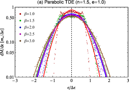
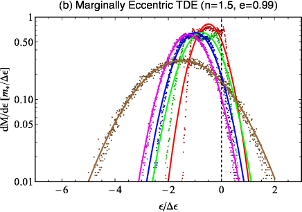
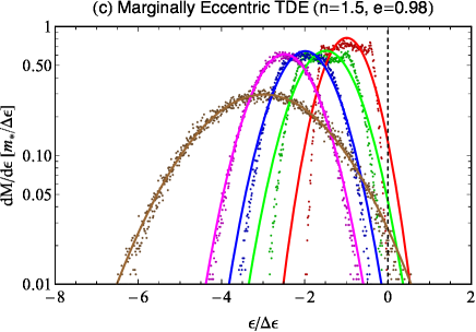
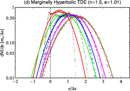
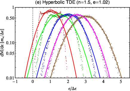
Figure 1: Simulated energy distribution of stellar debris for a $n=1.5$ polytrope (the differential debris mass is normalized by $m_{*}/\Delta\epsilon$). Each panel shows a different orbital eccentricity. The different colors correspond to different penetration factors ($\beta$). The solid lines are Gaussian fits to the simulation data.

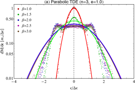
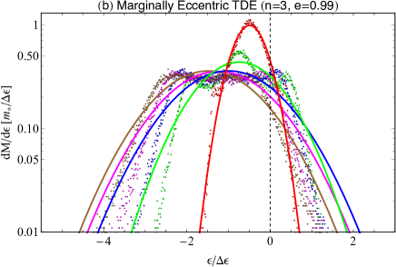
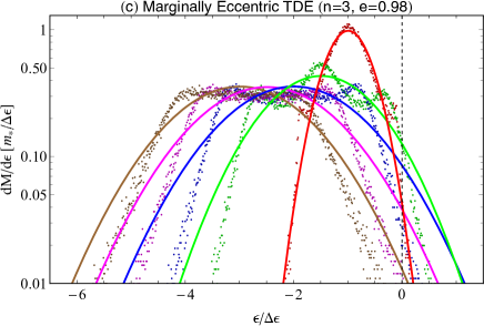
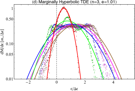
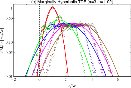
Figure 2: The same format as Figure 1, but for the case of $n=3$

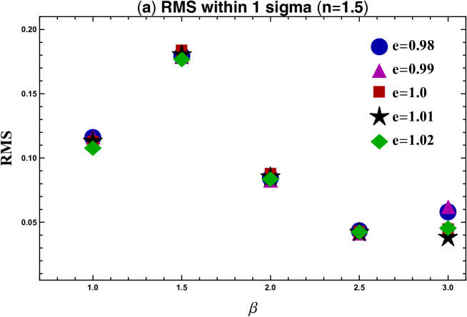
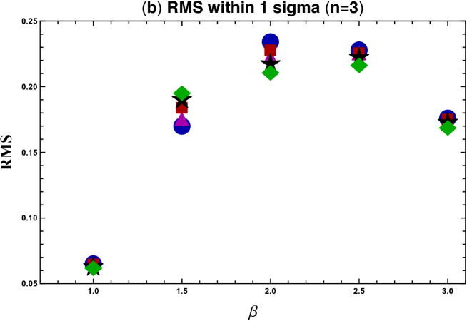
Figure 3: The root-mean square (RMS) between simulated data points and the Gaussian-fitted curves. Panels (a) and (b) panel show a $n=1.5$ and $n=3$ polytrope cases, respectively. The definition of RMS is shown in the second paragraph of Section 3.1.

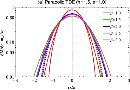
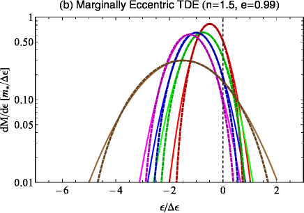
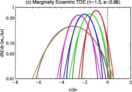
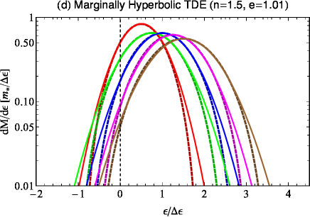
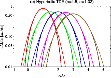
Figure 4: Comparison between the Gaussian fits to the simulation data and the corresponding semi-analytical distributions for an $n=1.5$ polytrope. Each panel shows a different orbital eccentricity. The solid and dashed lines show the Gaussian-fits and the semi-analytical distributions, respectively.

The color format of each line is the same as that of Figure 1.

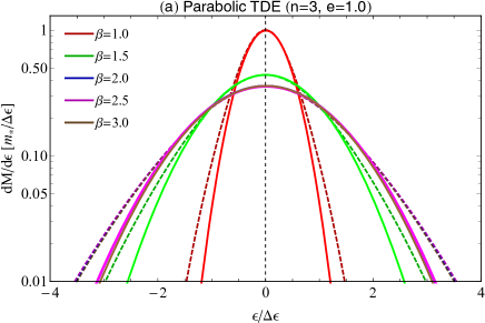
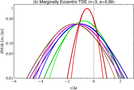
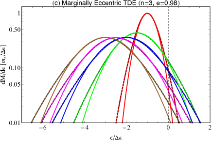
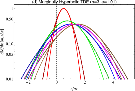
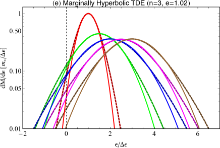
Figure 5: The same format as Figure 2, but for the case of $n=3$

3.2 Evaluation of tidal spread energy index: k

Assuming that the standard deviation of the Gaussian-fitted curve, $\Delta\mathcal{E}_{\rm sim}$, corresponds to the analytical spread energy $\Delta\mathcal{E}$, we can evaluate the power-law index of spread in tidal energy from equation (2) by

$$k=\frac{\log(\Delta\mathcal{E}_{\rm sim}/\Delta\epsilon)}{\log\beta}.$$ (26)

Figure 6 shows the dependence of the simulated spread energy on the penetration factor. Panels (a) and (b) show $\beta$-dependence of $\Delta\mathcal{E}_{\rm sim}/\Delta\mathcal{E}$ for the $n=1.5$ and $n=3$ cases, respectively. Panels (c) and (d) depict $\beta$-dependence of $\Delta\mathcal{E}_{\rm sim}/\Delta\epsilon$ for the $n=1.5$ and $n=3$ cases, respectively. In each panel, the blue circles, magenta triangles, red squares, black stars and green rhombuses represent results of $e=0.98$, $0.99$, $1.0$, $1.01$ and $1.02$, respectively. We find from panels (a) and (b) that the simulated spread energies are in good agreement with the analytical values for the $n=1.5$ and $n=3$ cases, although the error of $2\%$ is obtained for $\beta=1$. In addition, $\Delta\mathcal{E}_{\rm sim}/\Delta\epsilon$ slightly increases for $\beta=1$ as the orbital eccentricity decreases. We also find from panels (c) and (d) that the simulated spread energy, overall, increases beyond $\Delta\epsilon$ as the penetration factor increases.

$k$ with different penetration factors for the $n=1.5$ and $n=3$ cases, respectively. Panels (a) to (d) show results for $\beta=1.5,\beta=2,\beta=2.5$, and $\beta=3$, respectively. These two figures show that the value of $k$ is distributed between $0.2$ and $0.9$ for $n=1.5$, while the value of $k$ takes between $0.95$ and $2.2$ for the $n=3$ case. The detailed values of $k$ can be seen at the sixth column of Tables 1 and 2. We also find that the value of $k$ is larger than 2 only for the $\beta=1.5$ and $n=3$ case.

Figure 7 depicts the dependence of the tidal spread energy index on the orbital eccentricity with different penetration factors: $\beta=1.5,\beta=2,\beta=2.5$, and $\beta=3$. Each panel shows a different polytrope. These two figures show that the value of $k$ is distributed between $0.2$ and $0.9$ for $n=1.5$, while the value of $k$ takes between $0.95$ and $2.2$ for the $n=3$ case. The detailed values of $k$ can be seen at the sixth column of Tables 1 and 2. It is found from panel (b) that the value of $k$ is higher as $\beta$ is smaller for a $n=3$ polytrope, and this tendency is independent of the orbital eccentricity. We also find that the value of $k$ can be larger than 2 only for the $\beta=1.5$ and $n=3$ case.

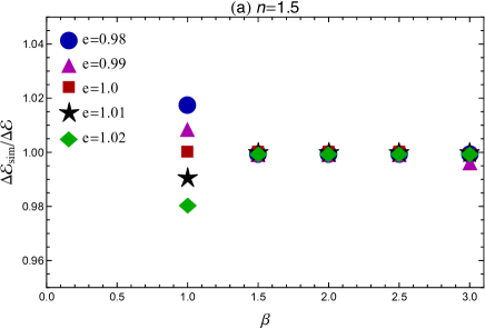
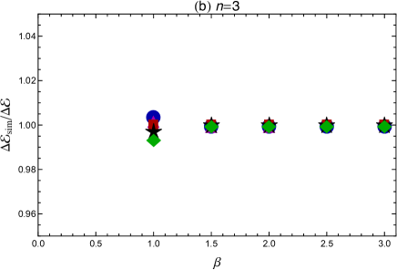
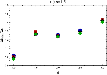
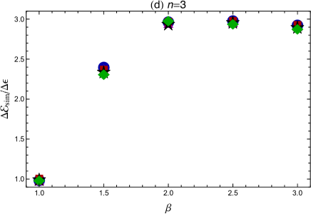
Figure 6: Dependence of the simulated spread energy on the penetration factor. Panels (a) and (b) show $\beta$-dependence of $\Delta\mathcal{E}_{\rm sim}/\Delta\mathcal{E}$ for the $n=1.5$ and $n=3$ cases, respectively. Panels (c) and (d) depict $\beta$-dependence of $\Delta\mathcal{E}_{\rm sim}/\Delta\epsilon$ for the $n=1.5$ and $n=3$ cases, respectively. Note that the relation between respective normalization is given by $\Delta\mathcal{E}=\Delta\epsilon\,\beta^{k}$ (see also equation 2). In each panel, the blue circles, magenta triangles, red squares, black stars, and green rhombuses represent results for $e=0.98$, $0.99$, $1.0$, $1.01$ and $1.02$, respectively.

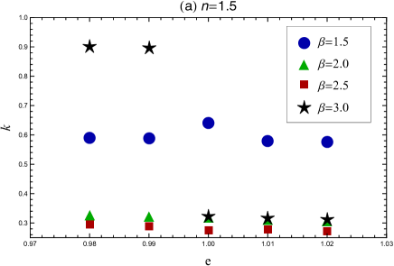
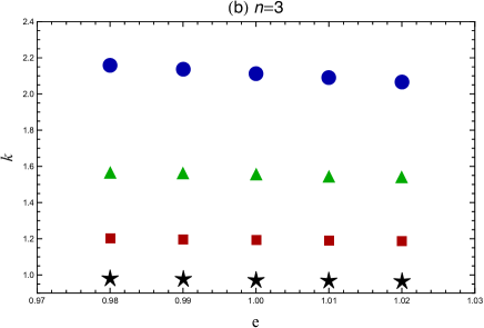
Figure 7: Orbital eccentricity dependence of the tidal spread energy index. Panels (a) and (b) represent it for the $n=1.5$ and $n=3$ cases, respectively. The blue circles, green triangles, red squares, and black stars denote the value of $k$ for $\beta=1.5$, $\beta=2$, $\beta=2.5$, and $\beta=3$, respectively.

3.3 Mass fallback rates

In this section, we evaluate the mass fallback rate of each model by using equation (4), where $dM/d\epsilon$ is given by the Gaussian fitted curves.

Figures 8 and 9 depict the Gaussian-fitted mass fallback rates for $n=1.5$ and $n=3$ polytropes, respectively. The red and blue curves represent the mass fallback rates of $\beta=1$ and $\beta=2.5$ in Figure 8, while they correspond to the $\beta=1$ and $\beta=3$ cases in Figure 9. Panels (a)-(d) depict the mass fallback rate of the parabolic TDE ($e=1.0$), marginally eccentric TDEs ($e=0.99$ and $e=0.98$), and the marginally hyperbolic TDE ($e=1.01$), respectively. The figures indicate that the peak of the mass fallback rate is higher as $\beta$ is higher, except for the marginally hyperbolic TDE of the $n=1.5$ case. This implies that the integral part of equation 25 (i.e., stellar density profile) more tightly correlates with the penetration factor compared with the $1/\beta^{k}$ term. The reason why the $\beta=1$ rate is overall higher than the $\beta=2.5$ rate for the marginally hyperbolic TDE is that the amount of the bound debris of $\beta=1$ is larger than that of $\beta=2.5$ (see Panel (d) of Figure 1). Overall, the mass fallback rates of marginally eccentric TDEs are an order of magnitude or more larger than those of the parabolic TDE, while the mass fallback rates of the marginally hyperbolic TDEs are less than or comparable to the Eddington rate and about one or a few orders of magnitude smaller than those of the parabolic TDEs.

Figure 10 depicts the slope of the Gaussian-fitted mass fallback rate as a function of time normalized by $t_{\rm mtb}$ for the case of a $n=1.5$ polytrope. Assuming that $dM/dt=At^{s}$, the slope of the mass fallback rate is given by

$$s=t\left(\frac{d^{2}M/dt^{2}}{dM/dt}\right),$$ (27)

where the proportionality coefficient, $A$, is a constant value. The solid blue, magenta, red, and black lines represents the slope of $e=0.98$, $e=0.99$, $e=1.0$, and $e=1.01$ cases, respectively, whereas the dashed line denotes the asymptotic slope of the mass fallback rate for the standard case, $-5/3$. Each panel depicts a different penetration factor. We find that the mass fallback rates of all types of TDEs are flatter than $t^{-5/3}$ at early times, while they are different at very late times for respective TDEs. The mass fallback rate asymptotically approaches to $t^{-5/3}$ for parabolic TDEs, is steeper than $t^{-5/3}$ for marginally eccentric TDEs, and is flatter for marginally hyperbolic TDEs. The time evolution of the slope in the $n=3$ case is qualitatively same as the evolution of the slope in the $n=1.5$ case as shown in Figure 11.

These outcomes are theoretically explained in the following way. Assuming $dM/d\epsilon=B{t}^{\alpha}$ ($B>1$), the slope of the mass fallback rate can be written by

$$s=\alpha-\frac{5}{3},$$ (28)

where we adopt the Keplerian third law to equation (4). Equation (28) indicates that the mass fallback rate is flatter (steeper) than $t^{-5/3}$ if $\alpha$ is positive (negative). Because $d^{2}M/d\epsilon^{2}=3\left(2\pi GM_{\rm bh}\right)^{-2/3}B\alpha t^{\alpha+2/3}$ where we used equation (6) for the derivation, $\alpha$ should be positive (negative) if the slope of $dM/d\epsilon$ about $\epsilon$ is positive (negative). It is clearly seen from Figure 1 that since the inclination of $dM/d\epsilon$ at the far negative side of $\epsilon$ is positive for all types of TDEs and all the given range of the penetration factor, $\alpha$ should be positive at early times. That is why the mass fallback rate is, independently of $\beta$, flatter than $t^{-5/3}$ at early times for all types of TDEs. On the other hand, it is clear from Figure 1 that the inclination of $dM/d\epsilon$ of parabolic TDEs is nearly flat at zero energy so that $\alpha\approx 0$ for all the given range of the penetration factor. Thus, the asymptotic slope of the mass fallback rate should be, independently of $\beta$, $-5/3$ at late times. In marginally eccentric TDEs, the inclination of $dM/d\epsilon$ is negative at zero energy (i.e., $\alpha<0$) for all the given range of the penetration factor so that the asymptotic slope is steeper than $-5/3$ at late times. In marginally hyperbolic TDEs, the inclination of $dM/d\epsilon$ is positive at zero energy (i.e., $\alpha>0$) for all the given range of the penetration factor so that the asymptotic slope is flatter than $-5/3$ at late times.

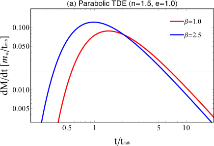
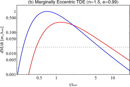
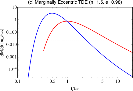
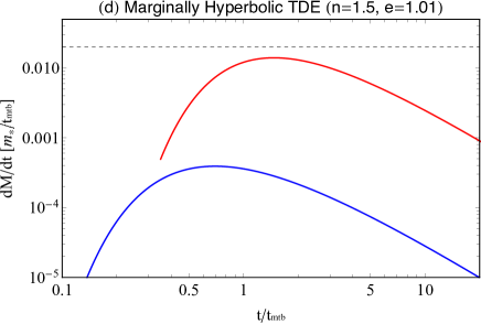
Figure 8: Gaussian-fitted mass fallback rates for a n=1.5 polytrope. They are normalized by $m_{*}/t_{\rm tmb}=0.11\,M_{\odot}/{\rm yr}\left(M_{\rm bh}/10^{6}M_{\odot}\right)^{-1/2}\left(M_{*}/M_{\odot}\right)\left(r_{*}/R_{\odot}\right)^{-3/2}\left(\beta/1\right)^{3k/2}$, where $k$ is obtained from Table 1. The red and blue solid lines show the normalized mass fallback rates of $\beta=1$ and $\beta=2.5$, respectively. The dashed line shows the normalized Eddington accretion rate. Each panel shows a different orbital eccentricity.

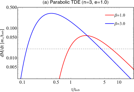
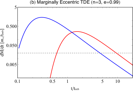
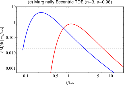
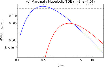
Figure 9: The same format as Figure 8, but for the $n=3$ case. The red and blue solid lines show the normalized mass fallback rates of $\beta=1$ and $\beta=3$, respectively.

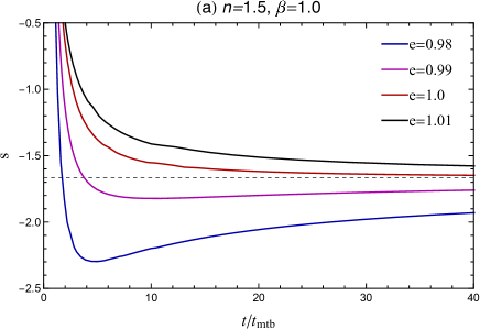
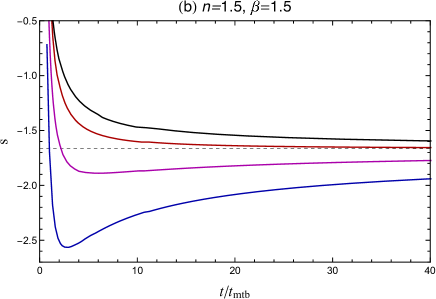
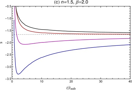
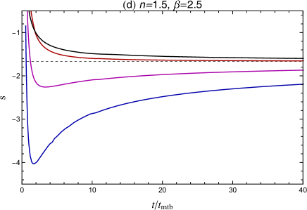
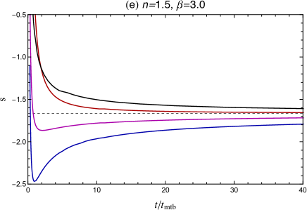
Figure 10: The slope of the Gaussian-fitted mass fallback rate as a function of time normalized by $t_{\rm mtb}$ for a $n=1.5$ polytrope. Each panel shows a different penetration factor. The blue, magenta, red, and black solid lines denote the slopes of $e=0.98$, $e=0.99$, $e=1.0$, and $e=1.01$, respectively. The dashed line represents $-5/3$, which is the slope of a standard TDE.

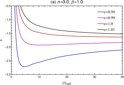
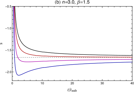
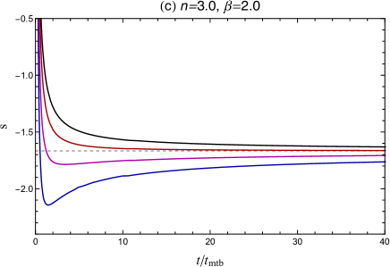
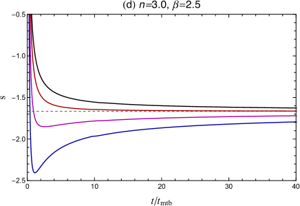
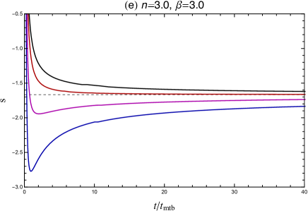
Figure 11: The same format as Figure 10, but for the $n=3$ case.

4 Discussion and Conclusions

We have revisited the mass fallback rates of marginally bound to unbound TDEs by taking account of the penetration factor ($\beta$), tidal spread energy index ($k$), orbital eccentricity ($e$), and stellar density profile with a polytropic index ($n$). We have compared the semi-analytical solutions with 3D SPH simulation results. Our primary conclusions are summarized as follows:

1. We have analytically derived the formulations of both the differential mass distribution and corresponding mass fallback rate and obtained the semi-analytical solutions for them. Both the differential mass distribution and corresponding mass fallback rate depend on the penetration factor, tidal spread energy index, orbital eccentricity (or semi-major axis), and stellar density profile (see equations 11 and 23 for differential mass distributions and equations 13 and 25 for mass fallback rates).

2. The differential mass distributions obtained by the SPH simulations show good agreement with the Gaussian-fitted curves, with errors of $\sim 5\%$ to $18\%$ for $n=1.5$, and $\sim 7\%$ to $24\%$ for $n=3$. We find that the Gaussian-fitted curves are in good agreement with the semi-analytical solutions, indicating that the analytically derived mass fallback rates can match the simulated rates within the range of the fitting accuracy.

3. The simulated spread in debris energy is larger than $\Delta\epsilon=GM_{\rm bh}/r_{\rm t}(r_{*}/r_{\rm t})$ as the penetration factor increases for all the cases, which is consistent with our assumption that the spread in debris energy is proportional to $\beta^{k}$ (see also equation (4) of Stone et al. 2013). While the tidal spread energy index is distributed over $0.27\lesssim{k}\lesssim 0.9$ for $n=1.5$ case for any value of $\beta$ and $e$, it is distributed over $0.97\lesssim{k}\lesssim 1.58$ for $n=3$ and any value of $\beta$ and $e$ except for the $\beta=1.5$ case. In this case, $k$ ranges from $2.08$ to $2.17$ depending on the orbital eccentricity.

4. We have updated the two critical eccentricities to classify five types of TDEs (see also Hayasaki et al. 2018), based on the spread in energy being proportional to $\beta^{k}$, as follows: $e_{\rm crit,1}=1-2(M_{\rm bn}/m_{*})^{-1/3}\beta^{k-1}$ and $e_{\rm crit,2}=1+2(M_{\rm bh}/m_{*})^{-1/3}\beta^{k-1}$ (see equation 20). Again, TDEs can be classified by five different types: eccentric ($e<e_{\rm crit,1}$), marginally eccentric ($e_{\rm crit,1}\lesssim{e}<1$), purely parabolic ($e=1$), marginally hyperbolic ($1<e<e_{\rm crit,2}$), and hyperbolic ($e\gtrsim{e_{\rm crit,2}}$) TDEs, respectively.

5. The mass fallback rates of the marginally eccentric TDEs are an order of magnitude or more larger than those of the parabolic TDEs, while the mass fallback rates of the marginally hyperbolic TDEs are less than or comparable to the Eddington rate and about one or a few orders of magnitude smaller than those of the parabolic TDEs.

6. We find that the mass fallback rates of all the types of TDEs are flatter than $t^{-5/3}$ at early times, while they are different at late times for the respective TDEs. The mass fallback rate asymptotically approaches to $t^{-5/3}$ for the parabolic TDEs, is steeper than $t^{-5/3}$ for the marginally eccentric TDEs, and is flatter for the marginally hyperbolic TDEs. The flatter nature at early times is because the inclination of the differential mass-energy distribution at the far side of negative debris energy is positive, while the steeper (flatter) nature at late times is because it is negative (positive) at zero energy. The reason why the asymptotic slope is $-5/3$ is that the slope of the differential mass distribution at zero energy is nearly flat (see also the detailed argument in the last two paragraphs of Section 3.3).

7. When the orbital eccentricity ranges for $1.0<e<e_{\rm crit,2}$ (i.e., marginally hyperbolic TDEs), only a little fraction of stellar mass can fall back to the black hole, which leads to the formation of advection dominated accretion flow (ADAF) or radiatively inefficient accretion flows (RIAF). The marginally hyperbolic TDEs can be an origin of ADAFs (or RIAFs) around dormant SMBHs. If the orbital eccentricity is more than $e_{\rm crit,2}$ (i.e., hyperbolic TDEs), no stellar debris can fall back to the black hole, which leads to a failed TDE.

Given the black hole mass, stellar mass and mass, and stellar density profile with a polytrope index, we see from Figures 8 and 9 that the mass fallback rate depends on the orbital eccentricity and penetration factor, and the orbital eccentricity enhances the peak of mass fallback rate than the penetration factor. The peak of the mass fallback rate can change by orders of magnitude over the range of $0.98\leq{e}\leq 1.01$ for both $n=1.5$ and $n=3$ cases. On the other hand, the mass fallback rate also strongly depends on the stellar types (i.e., stellar mass and radius): a white dwarf disruption shows a much larger fallback rate than the main sequence cases, whereas a red giant disruption represents a significantly lower rate (Law-Smith et al., 2017). TDEs of different stellar types are distinguishable, e.g., through the spectral line diagnosis because these stars have different compositions. The degeneracy between the stellar type and the orbital eccentricity should, then, be solvable by comparison with the TDEs of the same stellar types.

Partial tidal disruptions are the events where the outer layers of a star are tidally stripped by the black hole tidal forces. According to Guillochon & Ramirez-Ruiz (2013); Mainetti et al. (2017), a star can be partially disrupted if $\beta\lesssim 0.9$ for a $n=1.5$ polytrope and if $\beta\lesssim 2.0$ for a $n=3$ polytrope. No partial tidal disruption is seen for n=1.5 because of $\beta\geq 1.0$ in our simulations, while a star should be partially disrupted for the $n=3$ case with $\beta=1.0$ and $\beta=1.5$. In these cases, the mass fallback rate is thought to be asymptotically proportional to $t^{-9/4}$ (Guillochon & Ramirez-Ruiz, 2013; Coughlin & Nixon, 2019) because of the influence of the survived core on the stellar debris. However, the asymptotic slope of the mass fallback rate is $-5/3$ in our parabolic TDE case and is steeper only for the marginally eccentric TDEs. It suggests that there can be a degeneracy between the partial disruption of stars on parabolic orbits and marginally eccentric TDEs. We will study the partial disruption of stars on bound orbits to examine whether this degeneracy is solvable in a forthcoming paper.

Recent observations suggest that the peak luminosities of some candidates are significantly sub-Eddington in optical/UV (Hung et al., 2017; Mockler et al., 2019) and X-ray TDEs (Auchettl et al., 2017). These are inconsistent with the assumption that the bolometric luminosity is proportional to the mass fallback rate because the mass fallback rate significantly exceeds the Eddington accretion rate in the case of main-sequence star disruptions. Two main ideas to solve this problem have been proposed. One is the partial TDEs, where the mass fallback rate can be lower (Ivanov & Novikov, 2001; Guillochon & Ramirez-Ruiz, 2013). Another idea is that the radiative efficiency is very low for an elliptical disk accretion (Svirski et al., 2017). We propose a new approach that tidal disruption of stars on marginally hyperbolic orbits causes the low luminosity TDEs. As future works, this possibility should be tested by comparing it with the other two existing ideas.

If $4\lesssim\beta\lesssim\beta_{\rm max}$, where $\beta_{\rm max}=r_{\rm t}/r_{\rm S}\approx 24\,(M_{\rm bh}/10^{6}\,M_{\odot})^{-2/3}(m_{*}/M_{\odot})^{-1/3}(r_{*}/R_{\odot})$ is the maximum possible value of the penetration factor, the general relativistic (GR) effects get significantly important. In this case, the spread in tidal energy would not follow the simple power law of the penetration factor anymore. For example, if $\beta=10$ and $k\sim 2$, we are not sure if the spread in debris energy can be 100 times larger than the standard case, as predicted by the simple scaling (see equation 2). It is also unclear how high and steep the early time mass fallback rate is in this case. We will examine how much GR can affect $\beta$-dependence of spread in debris energy in tidal disruption of such a deep-plunging star, although some existing studies show deviation from the scaling law (Evans et al., 2015; Darbha et al., 2019; Steinberg et al., 2019).

Hayasaki & Yamazaki (2019) proposed that high-energy neutrinos with $\sim 7.5\,{\rm TeV}\,(M_{\rm bh}/10^{6}\,M_{\odot})^{5/3}$ can be emitted from an ADAF and/or RIAF formed after tidal disruption of a star by the decay of charged pions originated in ultra-relativistic protons. In the standard TDE theory, the RIAF phase would start at $t_{\rm RIAF}\sim 10^{10}\,{\rm s}$ for $10^{6}\,M_{\odot}$ black hole after a solar-type star disruption. For marginally unbound TDEs, the RIAF phase would start at about four orders of magnitude earlier than the standard case, i.e., $t_{\rm RIAF}\sim 10^{6}\,{\rm s}$ for $10^{6}\,M_{\odot}$ black hole and a solar-type star. Because the neutrino energy generation rate is estimated to be $L_{\nu}{t}_{\rm RIAF}\mathcal{R}$, where $L_{\nu}$ and $\mathcal{R}$ are the neutrino luminosity and the TDE rate respectively, such a short timescale can significantly enhance the energy generation rate even if the event rate of marginally hyperbolic TDEs would be subdominant.

References

- Alexander et al. (2016) Alexander, K. D., Berger, E., Guillochon, J., Zauderer, B. A., & Williams, P. K. G. 2016, ApJ, 819, L25
- Arcavi et al. (2014) Arcavi I. et al., 2014, ApJ, 793, 38
- Auchettl et al. (2017) Auchettl, K., Guillochon, J., & Ramirez-Ruiz, E. 2017, ApJ, 838, 149
- Bate et al. (1995) Bate, M. R., Bonnel, I. A., Price, N.M., 1995, MNRAS, 277, 362
- Bate (1995) Bate, M. R., 1995, Ph.D. Thesis, ch.2, 30-31
- Benz (1990) Benz W., 1990, in the Numerical Modeling of Nonlinear Steller Pulsations: Problems and Prospects, ed. Buchler, R.J. (Dordrecht: Kluwer Academic Publishers), 269
- Benz et al. (1990) Benz, W., Bowers, R.L., Cameron, A.G.W., Press, W.H., 1990, ApJ, 348, 647
- Bonnerot et al. (2016) Bonnerot, C. et al, 2016, MNRAS, 455, 2253
- Brown et al. (2015) Brown, G. C., Levan, A. J., Stanway, E. R., et al. 2015, MNRAS, 452, 4297
- Burrows et al. (2011) Burrows D. N. et al., 2011, Nature 476, 421
- Cannizzo et al. (1990) Cannizzo, J. K., Lee, H. M., & Goodman, J. 1990, ApJ, 351, 38
- Cannizzo & Gehrels (2009) Cannizzo, J. K., & Gehrels, N. 2009, ApJ, 700, 1047
- Chandrasekhar (1967) Chandrasekhar, S. An Introduction to the Study of Stellar Structure. New York: Dover, pp. 84-182, 1967.
- Chornock et al. (2014) Chornock, R., Berger, E., Gezari, S., et al. 2014, ApJ, 780, 44
- Coughlin & Nixon (2019) Coughlin, E. R., & Nixon, C. J. 2019, ApJ, 883, L17
- Dai et al. (2015) Dai, L., McKinney, J. C., & Miller, M. C. 2015, ApJ, 812, L39
- Darbha et al. (2019) Darbha, S., Coughlin, E. R., Kasen, D., et al. 2019, MNRAS, 488, 5267
- Donley et al. (2002) Donley J. L., Brandt W. N., Eracleous M., Boller T., 2002, AJ, 124, 1308
- Evans & Kochanek (1989) Evans C.R., Kochanek C.S., 1989, ApJ, 346, L13
- Evans et al. (2015) Evans, C., Laguna, P., & Eracleous, M. 2015, ApJ, 805, L19
- Esquej et al. (2008) Esquej, P., Saxton, R. D., Komossa, S., et al. 2008, A&A, 489, 543
- Farrar & Piran (2014) Farrar, G. R., & Piran, T. 2014, arXiv:1411.0704
- Gezari et al. (2006) Gezari, S., Martin, D. C., Milliard, B., et al. 2006, ApJ, 653, L25
- Gezari et al. (2008) Gezari, S., Basa, S., Martin, D. C., et al. 2008, ApJ, 676, 944-969
- Gezari et al. (2012) Gezari S. et al., 2012, Nature, 485, 217
- Gezari et al. (2015) Gezari, S., Chornock, R., Lawrence, A., et al. 2015, ApJ, 815, L5
- Guillochon & Ramirez-Ruiz (2013) Guillochon, J., & Ramirez-Ruiz, E. 2013, ApJ, 767, 25
- Hayasaki et al. (2013) Hayasaki, K., Stone, N., Loeb, A. 2013, MNRAS, 434, 909
- Hayasaki et al. (2016) Hayasaki, K., Stone, N., Loeb, A. 2016, MNRAS, 461, 3760
- Hayasaki et al. (2018) Hayasaki, K., Zhong, S., Li, S., Spurzem R. 2018, ApJ, 855, 129