Optimal Approximate Sampling from Discrete Probability Distributions

Abstract.

This paper addresses a fundamental problem in random variate generation: given access to a random source that emits a stream of independent fair bits, what is the most accurate and entropy-efficient algorithm for sampling from a discrete probability distribution $(p_{1},\dots,p_{n})$, where the probabilities of the output distribution $(\hat{p}_{1},\dots,\hat{p}_{n})$ of the sampling algorithm must be specified using at most $k$ bits of precision? We present a theoretical framework for formulating this problem and provide new techniques for finding sampling algorithms that are optimal both statistically (in the sense of sampling accuracy) and information-theoretically (in the sense of entropy consumption). We leverage these results to build a system that, for a broad family of measures of statistical accuracy, delivers a sampling algorithm whose expected entropy usage is minimal among those that induce the same distribution (i.e., is “entropy-optimal”) and whose output distribution $(\hat{p}_{1},\dots,\hat{p}_{n})$ is a closest approximation to the target distribution $(p_{1},\dots,p_{n})$ among all entropy-optimal sampling algorithms that operate within the specified $k$-bit precision. This optimal approximate sampler is also a closer approximation than any (possibly entropy-suboptimal) sampler that consumes a bounded amount of entropy with the specified precision, a class which includes floating-point implementations of inversion sampling and related methods found in many software libraries. We evaluate the accuracy, entropy consumption, precision requirements, and wall-clock runtime of our optimal approximate sampling algorithms on a broad set of distributions, demonstrating the ways that they are superior to existing approximate samplers and establishing that they often consume significantly fewer resources than are needed by exact samplers.

1. Introduction

Sampling from discrete probability distributions is a fundamental activity in fields such as statistics (Devroye, 1986), operations research (Harling, 1958), statistical physics (Binder, 1986), financial engineering (Glasserman, 2003), and general scientific computing (Liu, 2001). Recognizing the importance of sampling from discrete probability distributions, widely-used language platforms (Lea, 1992; MathWorks, 1993; R Core Team, 2014) typically implement algorithms for sampling from discrete distributions. As Monte Carlo methods move towards sampling billions of random variates per second (Djuric, 2019), there is an increasing need for sampling algorithms that are both efficient (in terms of the number of random bits they consume to generate a sample) and accurate (in terms of the statistical sampling error of the generated random variates with respect to the intended probability distribution). For example, in fields such as lattice-based cryptography and probabilistic hardware (de Schryver et al., 2012; Roy et al., 2013; Dwarakanath and Galbraith, 2014; Folláth, 2014; Mansinghka and Jonas, 2014; Du and Bai, 2015), the number of random bits consumed per sample, the size of the registers that store and manipulate the probability values, and the sampling error due to approximate representations of numbers are all fundamental design considerations.

We evaluate sampling algorithms for discrete probability distributions according to three criteria: (1) the entropy consumption of the sampling algorithm, as measured by the average number of random bits consumed from the source to produce a single sample (Definition 2.5); (2) the error of the sampling algorithm, which measures how closely the sampled probability distribution matches the specified distribution, using one of a family of statistical divergences (Definition 4.2); and (3) the precision required to implement the sampler, as measured by the minimum number of binary digits needed to represent each probability in the implemented distribution (Definition 2.13).

Let $(M_{1},\dots,M_{n})$ be a list of $n$ positive integers which sum to $Z$ and write $\mathbf{p}\coloneqq(p_{1},\dots,p_{n})$ for the discrete probability distribution over the set $[n]\coloneqq\{1,\dots,n\}$ defined by $p_{i}\coloneqq M_{i}/Z$ $(i=1,\dots,n)$. We distinguish between two types of algorithms for sampling from $\mathbf{p}$: (i) exact samplers, where the probability of returning $i$ is precisely equal to $p_{i}$ (i.e., zero sampling error); and (ii) approximate samplers, where the probability of returning $i$ is $\hat{p}_{i}\approx p_{i}$ (i.e., non-zero sampling error). In exact sampling, the numerical precision needed to represent the output probabilities of the sampler varies with the values $p_{i}$ of the target distribution; we say these methods need arbitrary precision. In approximate sampling, on the other hand, the numerical precision needed to represent the output probabilities $\hat{p}_{i}$ of the sampler is fixed independently of the $p_{i}$ (by constraints such as the register width of a hardware circuit or arithmetic system implemented in software); we say these methods need limited precision. We next discuss the tradeoffs between entropy consumption, sampling error, and numerical precision made by exact and approximate samplers.

1.1. Existing Methods for Exact and Approximate Sampling

Inversion sampling is a universal method for obtaining a random sample from any probability distribution (Devroye, 1986, Theorem 2.1). The inversion method is based on the identity that if $U$ is a uniformly distributed real number on the unit interval $[0,1]$, then

(1) $$\textstyle\Pr\left[\sum_{i=1}^{j-1}p_{i}\leq U<\sum_{i=1}^{j}p_{i}\right]=p_{j} (j=1,\dots,n).$$

Knuth and Yao (1976) present a seminal theoretical framework for constructing an exact sampler for any discrete probability distribution. The sampler consumes, in expectation, the least amount of random bits per sample among the class of all exact sampling algorithms (Theorem 2.9). The Knuth and Yao sampler is an implementation of the inversion method which compares (lazily sampled) bits in the binary expansion of $U$ to the bits in the binary expansion of the $p_{i}$. Despite its minimal entropy consumption and zero sampling error, the method requires arbitrary precision and the computational resources needed to implement the sampler are often exponentially larger than the number of bits needed to encode the probabilities (Theorem 3.5), even for typical distributions (Table 4). In addition to potentially requiring more resources than are available even on modern machines, the framework is presented from a theoretical perspective without readily-programmable implementations of the sampler, which has further limited its general application.

The rejection method (Devroye, 1986), shown in Algorithm 1, is another technique for exact sampling where, unlike the Knuth and Yao method, the required precision is polynomial in the number of bits needed to encode $\mathbf{p}$. Rejection sampling is exact, readily-programmable, and typically requires reasonable computational resources. However, it is highly entropy-inefficient and can consume exponentially more random bits than is necessary to generate a sample (Example 5.1).

We now discuss approximate sampling methods which use a limited amount of numerical precision that is specified independently of the target distribution $\mathbf{p}$. Several widely-used software systems such as the MATLAB Statistics Toolbox (MathWorks, 1993) and GNU C++ standard library (Lea, 1992) implement the inversion method based directly on Eq. (1), where a floating-point number $U^{\prime}$ is used to approximate the ideal real random variable $U$, as shown in Algorithm 2. These implementations have two fundamental deficiencies: first, the algorithm draws a fixed number of random bits (typically equal to the 32-bit or 64-bit word size of the machine) per sample to determine $U^{\prime}$, which may result in high approximation error (Section 2.4), is suboptimal in its use of entropy, and often incurs non-negligible computational overhead in practice; second, floating-point approximations for computing and comparing $U^{\prime}$ to running sums of $p_{i}$ produce significantly suboptimal sampling errors (Figure 3) and the theoretical properties are challenging to characterize (von Neumann, 1951; Devroye, 1982; Monahan, 1985). In particular, many of these approximate methods, unlike the method presented in this paper, are not straightforwardly described as producing samples from a distribution that is close to the target distribution with respect to a specified measure of statistical error and provide no optimality guarantees.

Algorithm 1 Rejection Sampling

Given probabilities $(M_{i}/Z)_{i=1}^{n}$: (1) Let $k$ be such that $2^{k-1}\,{<}\,Z\,{\leq}\,2^{k}$. (2) Draw a $k$-bit integer $W\in\{0,\dots,2^{k}-1\}$. (3) If $W\,{<}\,Z$, return integer $j\,{\in}\,[n]$ such that $\sum_{i=1}^{j-1}M_{i}\,{\leq}\,W\,{<}\,\sum_{i=1}^{j}M_{i}$; else go to 2.

Algorithm 2 Inversion Sampling

Given probabilities $(M_{i}/Z)_{i=1}^{n}$, precision $k$: (1) Draw a $k$-bit integer $W\in\{0,\dots,2^{k}-1\}$. (2) Let $U^{\prime}\coloneqq W/2^{k}$. (3) Return smallest integer $j\,{\in}\,[n]$ such that $U^{\prime}<\sum_{i=1}^{j}M_{i}/Z$.

The interval method (Han and Hoshi, 1997) is an implementation of the inversion method which, unlike the previous methods, lazily obtains a sequence $U_{i}$ of fair coin flips from the set $\{0,1\}$ and recursively partitions the unit interval until the outcome $j\in[n]$ can be determined. Han and Hoshi (1997) present an exact sampling algorithm (using arbitrary precision) and Uyematsu and Li (2003) present an approximate sampling algorithm (using limited precision). Although entropy consumed by the interval method is close to the optimal limits of Knuth and Yao (1976), the exact sampler uses several floating-point computations and has an expensive search loop during sampling (Devroye and Gravel, 2015, Algorithm 1). The limited-precision sampler is more entropy-efficient than the limited-precision inversion sampler (Table 2) but often incurs a higher error (Figure 3).

1.2. Optimal Approximate Sampling

This paper presents a novel class of algorithms for optimal approximate sampling from discrete probability distributions. Given a target distribution $\mathbf{p}\coloneqq(p_{1},\dots,p_{n})$, any measure of statistical error in the family of (1-1 transformations of) $f$-divergences (Definition 4.2), and a number $k$ specifying the allowed numerical precision, our system returns a sampler for $\mathbf{p}$ that is optimal in a very strong sense: it produces random variates with the minimal sampling error possible given the specified precision, among the class of all entropy-optimal samplers of this precision (Theorems 3.4 and 4.7). Moreover these samplers comprise, to the best of our knowledge, the first algorithms that, for any target distribution, measure of statistical accuracy, and specification of bit precision, provide rigorous guarantees on the entropy-optimality and the minimality of the sampling error.

The key idea is to first find a distribution $\hat{\mathbf{p}}\coloneqq(\hat{p}_{1},\dots,\hat{p}_{n})$ whose approximation error of $\mathbf{p}$ is minimal among the class of all distributions that can be sampled by any $k$-bit entropy-optimal sampler (Section 4). The second step is to explicitly construct an entropy-optimal sampler for the distribution $\hat{\mathbf{p}}$ (Section 5). In comparison with previous limited-precision samplers, our samplers are more entropy-efficient and more accurate than any sampler that always consumes at most $k$ random bits (Proposition 2.16), which includes any algorithm that uses a finite number of approximately uniform floating-point numbers (e.g., limited-precision inversion sampling and interval sampling). The time, space, and entropy resources required by our samplers can be significantly less than those required by the exact Knuth and Yao and rejection methods (Section 6.3), with an approximation error that decreases exponentially quickly with the amount of precision (Theorem 4.17).

The sampling algorithms delivered by our system are algorithmically efficient: they use integer arithmetic, admit straightforward implementations in software and probabilistic hardware systems, run in constant time with respect to the length $n$ of the target distribution and linearly in the entropy of the sampler, and can generate billions of random variates per second. In addition, we present scalable algorithms where, for a precision specification of $k$ bits, the runtime of finding the $n$ optimal approximate probabilities $\hat{\mathbf{p}}$ is order $n\log{n}$, and of building the corresponding sampler is order $nk$. Prototype implementations of the system in C and Python are available in the online artifact and at https://github.com/probcomp/optimal-approximate-sampling.

1.3. Contributions

The main contributions of this paper are:

Formulation of optimal approximate sampling algorithms for discrete distributions. This precise formulation allow us to rigorously study the notion of entropy consumption, statistical sampling error, and numerical precision. These three functional metrics are used to assess the entropy-efficiency, accuracy, and memory requirements of a sampling algorithm.

Theoretical results for the class of entropy-optimal sampling algorithms. For a specified precision, we characterize the set of output probability distributions achievable by any entropy-optimal sampler that operates within the given precision specification. We leverage these results to constrain the space of probability distributions for approximating a given target distribution to contain only those that correspond to limited-precision entropy-optimal samplers.

Algorithms for finding optimal approximations to discrete distributions. We present a new optimization algorithm that, given a target distribution $\mathbf{p}$, a measure of statistical divergence, and a precision specification, efficiently searches the combinatorially large space of entropy-optimal samplers of the given precision, to find a optimal approximation sampler that most accurately approximates the target distribution $\mathbf{p}$. We prove the correctness of the algorithm and analyze its runtime in terms of the size of the target distribution and precision specification.

Algorithms for constructing entropy-optimal sampling algorithms. We present detailed algorithms for sampling from any closest-approximation probability distribution $\hat{\mathbf{p}}$ in a way that is entropy-optimal, using the guarantees provided by the main theorems of Knuth and Yao (1976). Our prototype implementation can generate billions of random variates per second and executes between $1.5$x (for low-dimensional distributions) and $195$x (for high-dimensional distributions) faster than the limited-precision linear inversion sampler provided as part of the GNU C++ standard library (Lea, 1992).

Comparisons to baseline limited-precision sampling algorithms. For several common probability distributions, we empirically demonstrate that the proposed sampling algorithms consume less entropy and are up to 1000x—10000x more accurate than the limited-precision inversion sampler from the GNU C++ standard library (Lea, 1992) and interval algorithm (Uyematsu and Li, 2003). We also show that (i) our sampler scales more efficiently as the size of the target distribution grows; and (ii) using the information-theoretically minimal amount of bits per sample leads to up to 10x less wall-clock time spent calling the underlying pseudorandom number generator.

Comparisons to baseline exact sampling algorithms. We present a detailed study of the exact Knuth and Yao method, the rejection method, and the proposed method for a canonical discrete probability distribution. We demonstrate that our samplers can use 150x less random bits per sample than rejection sampling and many orders of magnitude less precision than exact Knuth and Yao sampling, and can (unlike exact sampling algorithms) trade off greater numerical precision in exchange for exponentially smaller sampling accuracy, all while remaining entropy-optimal.

The remainder of this paper is structured as follows: Section 2 describes the random bit model of computation for sampling algorithms and provides formal definitions used throughout the paper. Section 3 presents theoretical results on the class of entropy-optimal samplers which are leveraged in future sections. Section 4 presents an efficient algorithm for finding a closest-approximation distribution to any given target distribution. Section 5 presents algorithms for constructing entropy-optimal samplers. Section 6 investigates the properties of the optimal samplers and compares them to multiple existing sampling methods in terms of accuracy, precision, entropy, and runtime.

2. Computational models of sampling algorithms

In the algebraic model of computation over the real numbers (also known as the real RAM model (Blum et al., 1998)), a sampling algorithm has access to an ideal register machine that can (i) sample a real random variable $U$ uniformly distributed on the unit interval $[0,1]$ using a primitive called $\textsf{uniform}()$, which forms the basic unit of randomness; and (ii) store and perform algebraic operations on infinitely-precise real numbers in unit time (Devroye, 1986, Assumptions 1, 2, and 3). The algebraic model is useful for proving the correctness of exact mathematical transformations applied to a uniform random variate $U$ and for analyzing the algorithmic runtime and storage costs of preprocessing and sampling, assuming access to infinite amounts of entropy or precision (Walker, 1977; Vose, 1991; Smith, 2002; Bringmann and Panagiotou, 2017).

However, sampling algorithms that access an infinite amount of entropy and compute with infinite precision real arithmetic cannot be implemented on physical machines. In practice, these algorithms are implemented on machines which use a finite amount of entropy and compute with approximate real arithmetic (e.g., double-precision floating point). As a result, sampling algorithms typically have a non-zero sampling error, which is challenging to systematically assess in practice (Devroye, 1982). While the quality of sampling algorithms implemented in practice is often characterized using ad-hoc statistical goodness-of-fit tests on a large number of simulations (Walker, 1974; Leydold and Chaudhuri, 2014), these empirical metrics fail to give rigorous statistical guarantees about the accuracy and/or theoretical optimality of the algorithm (Monahan, 1985). In this paper, we consider an alternative computational model that is more appropriate in applications where limited numerical precision, sampling error, or entropy consumption are of interest.

2.1. The Random Bit Model

In the random bit model, introduced by von Neumann (1951), the basic unit of randomness is a random symbol in the set $\{0,1,\dots,b-1\}$ for some integer $b\geq 2$, obtained using a primitive called $\textsf{flip}()$. Since the random symbols are produced lazily by the source and the output of the sampling algorithm is a deterministic function of the discrete symbols, this model is suitable for analyzing entropy consumption and sampling error. In this paper, we consider the random bit model of computation where any sampling algorithm for a target distribution $\mathbf{p}$ over $[n]$ operates under the following assumptions:

1. each invocation of $\textsf{flip}()$ returns a single fair (unbiased) binary digit in $\{0,1\}$ (i.e., $b=2$);

2. the bits returned by separate invocations of $\textsf{flip}()$ are all mutually independent;

3. the output of the sampling algorithm is a single outcome in $[n]$, which is independent of all previous outputs of the algorithm; and

4. the output probabilities of the sampling algorithm can be specified using at most $k$ binary digits, where the numerical precision parameter $k$ is specified independently of the target distribution $\mathbf{p}$.

Several limited-precision algorithms for sampling from discrete probability distributions in the literature operate under assumptions similar to A1–A4; examples include samplers for the uniform (Lumbroso, 2013), discrete Gaussian (Folláth, 2014), geometric (Bringmann and Friedrich, 2013), random graph (Blanca and Mihail, 2012), and general discrete (Uyematsu and Li, 2003) distributions. Since these sampling algorithms use limited numerical precision that is specified independently of the target distribution (A4), they typically have some statistical sampling error.

We also note that several variants of the random bit model for random variate generation, which operate under different assumptions than A1–A4, have been thoroughly investigated in the literature. These variants include using a random source which provides flips of a biased $b$-sided coin (where the bias may be known or unknown); using a random source which provides non-i.i.d. symbols; sampling algorithms which return a random number of non-independent output symbols in each invocation; and/or sampling algorithms which use arithmetic operations whose numerical precision depends on the probabilities in the target distribution (von Neumann, 1951; Elias, 1972; Stout and Warren, 1984; Blum, 1986; Roche, 1991; Peres, 1992; Han and Verdú, 1993; Vembu and Verdú, 1995; Abrahams, 1996; Pae and Loui, 2006; Cicalese et al., 2006; Kozen, 2014; Kozen and Soloviev, 2018). For example, Pae and Loui (2006) solve the very general problem of optimally simulating an arbitrary target distribution using $k$ independent flips of a $b$-sided coin with unknown bias, where optimality is defined in the sense of the asymptotic ratio of output bits per input symbol. Kozen and Soloviev (2018) provide a unifying coalgebraic framework for implementing and composing entropy-preserving reductions between arbitrary input sources to output distributions, describe several concrete algorithms for reductions between random processes, and present bounds on the trade-off between the latency and asymptotic entropy-efficiency of these protocols.

The assumptions A1–A4 that we make in this paper are designed to explore a new set of trade-offs compared to those explored in previous works. More specifically, the current paper trades off accuracy with numerical precision in the non-asymptotic setting, while maintaining entropy-optimality of the output distribution, whereas the works of Pae and Loui (2006) and Kozen and Soloviev (2018), for example, trade off asymptotic entropy-efficiency with numerical precision, while maintaining perfect accuracy. The trade-offs we consider are motivated by the standard practice in numerical sampling libraries (Lea, 1992; MathWorks, 1993; R Core Team, 2014; Galassi et al., 2019), which (i) use an entropy source that provides independent fair bits (modulo the fact that they may use pseudorandom number generators); (ii) implement samplers that guarantee exactly one output symbol per invocation; (iii) implement samplers that have non-zero output error; and (iv) use arithmetic systems with a fixed amount of precision (using e.g., 32-bit or 64-bit floating point). For the trade-offs considered in this paper, we present results that conclusively solve the problem of finding entropy-optimal sampling algorithms operating within any precision specification that yield closest-approximation distributions among the class of all entropy-optimal samplers that also operate within the given precision. The next section formalizes these concepts.

2.2. Preliminaries

Definition 2.1 (Sampling algorithm).

Let $n\geq 1$ be an integer. A sampling algorithm, or sampler, $A:\biguplus_{k=1}^{\infty}\{0,1\}^{k}\to\{1,\dots,n,\bot\}$ is a map that sends each finite tuple of bits to either an outcome in $[n]$ or a special symbol $\bot$ that indicates more bits are needed to determine the final outcome.

Remark 2.2.

In Assumption A1 and Definition 2.1, the assumption that the source outputs binary digits in $\{0,1\}$ (i.e., $b=2$) is made without loss of generality. All the definitions and results in this paper generalize directly to the case of a source that outputs fair flips of any $b$-sided coin.

Knuth and Yao (1976) present a computational framework for expressing the set of all sampling algorithms for discrete probability distribution in the random bit model. Any sampling algorithm $A$ that draws random bits and returns an integer outcome $i$ with probability $p_{i}$ $(i=1,\dots,n)$ is equivalent to some (possibly infinite) binary tree $T$. Each internal node of $T$ has exactly 2 children and each leaf node is labeled with an outcome in $[n]$. The sampling algorithm starts at the root of $T$. It then draws a random bit $b$ from the source and takes the left branch if $b=0$ or the right branch if $b=1$. If the child node is a leaf node, the label assigned to that leaf is returned and the computation halts. Otherwise, the child node is an internal node, so a new random bit is drawn from the source and the process repeats. The next definition presents a state machine model that formally describes the behavior of any sampling algorithm in terms of such a computation tree.

Definition 2.3 (Discrete distribution generating tree).

Let $A$ be a sampling algorithm. The computational behavior of $A$ is described by a state machine $T=(S,r,n,c,\delta)$, called the discrete distribution generating (DDG) tree of $A$, where

• $S\subseteq\mathbb{N}$ is a set of states (nodes);

• $r\in S$ is a designated start node;

• $n\geq 1$ is an integer indicating the number of outcomes of the sampler;

• $c:S\to\{1,\dots,n\}\,\cup\,\{\mathsf{branch}\}$ is a function that labels each node as either a branch node or a terminal (leaf) node assigned to an outcome in $[n]$; and

• $\delta:S\times\{0,1\}\to S$ is a transition function that maps a node and a random bit to a new node.

Let $\mathbf{b}_{k}\coloneqq(b_{1},\dots,b_{k})\in\{0,1\}^{k}$ be a tuple of $k\geq 0$ bits, $i\in S$ a state, and $j\in\mathbb{N}$. The operational semantics of $T$ for a configuration $\langle i,j,\mathbf{b}_{k}\rangle$ of the state machine are defined by the following rules

(2) $$\left\langle{i,j,\mathbf{b}_{k}}\right\rangle_{T}\to\left\langle{\delta(i,b_{j+1}),{j+1},\mathbf{b}_{k}}\right\rangle_{T}0\leq j<k;\;c(i)=\mathsf{branch} \left\langle{i,j,\mathbf{b}_{k}}\right\rangle_{T}\to\bot k\leq j;\;c(i)=\mathsf{branch} \left\langle{i,j,\mathbf{b}_{k}}\right\rangle_{T}\to c(i)0\leq j\leq k;\;c(i)\in[n]$$

In Eq. (2), the arrow $\to$ defines a transition relation from the current configuration (i.e., state $i$, consumed bits $j$, and input bits $\mathbf{b}_{k}$) to either a new configuration (first rule) or to a terminal outcome in $\{1,\dots,n,\bot\}$ (second and third rules). The output of $A$ on input $\mathbf{b}_{k}$ is given by $A(\mathbf{b}_{k})\coloneqq\left\langle{r,0,\mathbf{b}_{k}}\right\rangle_{T}$.

Definition 2.4 (Output distribution).

Let $T$ be the DDG tree of a sampler $A$, $\mathbf{1}[\cdot]$ the indicator function, and $\mathbf{b}_{k}\sim\textsf{Uniform}\left(\{0,1\}^{k}\right)$ a random draw of $k\geq 0$ fair independent bits. Then

(3) $$\Pr[A(\mathbf{b}_{k})=i] =\frac{1}{2^{k}}\sum_{\mathbf{b}^{\prime}\in\{0,1\}^{k}}\mathbf{1}[\left\langle{(r,0,\mathbf{b}^{\prime})}\right\rangle_{T}=i] (i=1,\dots,n).$$

The overall probability of returning $$i \mathbf{b}_{\infty}$$, over an infinite length random stream from the source, is

(4) $$p_{i} \coloneqq\Pr[A(\mathbf{b}_{\infty})=i]=\lim_{k\to\infty}\Pr[A(\mathbf{b}_{k})=i] (i=1,\dots,n).$$

For each $k$ we have $\Pr[A(\mathbf{b}_{k})=\bot]=1-\sum_{i=1}^{n}\Pr[A(\mathbf{b}_{k})=i]$. The list of outcome probabilities $(p_{1},\dots,p_{n})$ defined in Eq. (4) is the called the output distribution of $T$, and we say that $T$ is well-formed whenever these probabilities sum to one (equivalently, whenever $A$ halts with probability one, so that $\Pr[A(\mathbf{b}_{\infty})=\bot]=0$).

Definition 2.5 (Number of consumed bits).

For each $k\geq 0$, let $\mathbf{b}_{k}\sim\textsf{Uniform}\left(\{0,1\}^{k}\right)$ be a random draw of $k$ bits from the source. The number of bits consumed by $A$ is a random variable defined by

(5) $$N_{k}(A,\mathbf{b}_{k})\coloneqq\min(k,\min\limits_{1\leq j\leq k}\{j\mid A(b_{1},\dots,b_{j})\in[n]\}) (k=0,1,\dots).$$

(where $\min(\varnothing)\coloneqq\infty$), which is precisely the (random) number of steps executed in the evaluation rules (2) on the (random) input $\mathbf{b}_{k}$. Furthermore, we define $N(A)\coloneqq\lim_{k\to\infty}N_{k}(A,\mathbf{b}_{k})$ to be the limiting number of bits per sample, which exists (in the extended reals) whenever $T$ is well-formed.

Definition 2.6 (Entropy (Shannon, 1948)).

Let $\mathbf{p}$ be a probability distribution over $[n]$. The Shannon entropy $H(\mathbf{p})\coloneqq\sum_{i=1}^{n}p_{i}\log(1/p_{i})$ is a measure of the stochasticity of $\mathbf{p}$ (unless otherwise noted, all instances of $\log$ are base 2). For each integer $n$, a deterministic distribution has minimal entropy ($H(\mathbf{p})=0$) and the uniform distribution has maximal entropy ($H(\mathbf{p})=\log(n)$).

Definition 2.7 (Entropy-optimal sampler).

A sampling algorithm $A$ (or DDG tree $T$) with output distribution $\mathbf{p}$ is called entropy-optimal if the expected number of random bits consumed from the source is minimal among all samplers (or DDG trees) that yield the same output distribution $\mathbf{p}$.

Definition 2.8 (Concise binary expansion).

We say that a binary expansion of a rational number is concise if its repeating part is not of the form $\overline{1}$. In other words, to be concise, the binary expansions of dyadic rationals must end in $\overline{0}$ rather than $\overline{1}$.

Theorem 2.9 (Knuth and Yao (1976)).

Let $\mathbf{p}\coloneqq(p_{1},\dots,p_{n})$ be a discrete probability distribution for some positive integer $n$. Let $A$ be an entropy-optimal sampler whose output distribution is equal to $\mathbf{p}$. Then the number of bits $N(A)$ consumed by $A$ satisfies $H(\mathbf{p})\leq\mathbb{E}[N(A)]<H(\mathbf{p})+2$. Further, the underlying DDG tree $T$ of $A$ contains exactly 1 leaf node labeled $i$ at level $j$ if and only if $p_{ij}=1$, where $(0.p_{i1}p_{i2}\dots)_{2}$ denotes the concise binary expansion of each $p_{i}$.

We next present three examples of target distributions and corresponding DDG trees that are both entropy-optimal, based on the construction from Theorem 2.9 and entropy-suboptimal. By Theorem 2.9, an entropy-optimal DDG tree for $\mathbf{p}$ can be constructed directly from a data structure called the binary probability matrix $\mathbf{P}$, whose entry $\mathbf{P}[i,j]$ corresponds to the $j$th bit in the concise binary expansion of $p_{i}$ ($i=1,\ldots,n;j\geq 0$). In general, the matrix $\mathbf{P}$ can contain infinitely many columns, but it can be finitely encoded when the probabilities of $\mathbf{p}$ are rational numbers.

In the case where each $p_{i}$ is dyadic, as in Example 2.10, we may instead work with the finite matrix $\mathbf{P}$ that omits those columns corresponding to a final $\overline{0}$ in every row, i.e., whose width is the maximum number of non-zero binary digits to the right of “$0.$” in a concise binary expansion of $p_{i}$.

Example 2.10.

$$\begin{bmatrix}p_{1}\\ p_{2}\\ p_{3}\end{bmatrix}=\begin{bmatrix}1/2\\ 1/4\\ 1/4\end{bmatrix}=\begin{bmatrix}.&1&0\\ .&0&1\\ .&0&1\\ \end{bmatrix}$$

Binary probability matrix

Entropy-optimal DDG tree

Entropy-suboptimal DDG tree

Consider the distribution $\mathbf{p}\coloneqq(1/2,1/4,1/4)$ over $\{1,2,3\}$. Since $p_{1}=(0.10)_{2}$ and $p_{2}=p_{3}=(0.01)_{2}$ are all dyadic, the finite matrix $\mathbf{P}$ has two columns and the entropy-optimal tree has three levels (the root is level zero). Also shown above is an entropy-suboptimal tree for $\mathbf{p}$.

Now consider the case where the values of $\mathbf{p}$ are all rational but not all dyadic, as in Example 2.11. Then the full binary probability matrix can be encoded using a probability “pseudomatrix” $\mathbf{P}$, which has a finite number of columns that contain the digits in the finite prefix and the infinitely-repeating suffix of the concise binary expansions (a horizontal bar is placed atop the columns that contain the repeating suffix). Similarly, the infinite-level DDG tree for $\mathbf{p}$ can be finitely encoded by using back-edges in a “pseudotree”. Note that the DDG trees from Definition 2.3 are technically pseudotrees of this form, where $\delta$ encodes back-edges that finitely encode infinite trees with repeating structure. The terms “trees” and “pseudotrees” are used interchangeably throughout the paper.

Example 2.11.

$$\begin{bmatrix}p_{1}\\ p_{2}\end{bmatrix}=\begin{bmatrix}3/10\\ 7/10\end{bmatrix}=\begin{bmatrix}.&0&\overline{1\;0\;0\;1}\,\\ .&1&\overline{0\;1\;1\;0}\,\\ \end{bmatrix}$$

Binary probability matrix

Entropy-optimal DDG tree

Entropy-suboptimal DDG tree

Consider the distribution $\mathbf{p}\coloneqq(3/10,7/10)$ over $\{1,2\}$. As $p_{1}$ and $p_{2}$ are non-dyadic rational numbers, their infinite binary expansions can be finitely encoded using a pseudotree. The (shortest) entropy-optimal pseudotree shown above has five levels and a back-edge (red) from level four to level one. This structure corresponds to the structure of $\mathbf{P}$, which has five columns and a prefix length of one, as indicated by the horizontal bar above the last four columns of the matrix.

If any probability $p_{i}$ is irrational, as in Example 2.12, then its concise binary expansion will not repeat, and so we must work with the full binary probability matrix, which has infinitely many columns. Any DDG tree for $\mathbf{p}$ has infinitely many levels, and neither the matrix nor the tree can be finitely encoded. Probability distributions whose samplers cannot be finitely encoded are not the focus of the sampling algorithms in this paper.

Example 2.12 (Knuth and Yao (1976)).

$$\begin{bmatrix}p_{1}\\ p_{2}\\ p_{3}\end{bmatrix}=\begin{bmatrix}1/\pi\\ 1/e\\ 1-1/\pi-1/e\end{bmatrix}=\begin{bmatrix}.&0&1&0&1&0&0&0&\dots\\ .&0&1&0&1&1&1&1&\dots\\ .&0&1&0&1&0&0&0&\dots\\ \end{bmatrix}$$

Binary probability matrix

Entropy-optimal DDG tree

Consider the distribution $\mathbf{p}\coloneqq(1/\pi,\,1/e,\,1-1/\pi-1/e)$ over $\{1,2,3\}$. The binary probability matrix has infinitely many columns and the corresponding DDG tree shown above has infinitely many levels, and neither can be finitely encoded.

2.3. Sampling Algorithms with Limited Computational Resources

The previous examples present three classes of sampling algorithms, which are mutually exclusive and collectively exhaustive: Example 2.10 shows a sampler that halts after consuming at most $k$ bits from the source and has a finite DDG tree; Example 2.11 shows a sampler that needs an unbounded number of bits from the source and has an infinite DDG tree that can be finitely encoded; and Example 2.12 shows a sampler that needs an unbounded number of bits from the source and has an infinite DDG tree that cannot be finitely encoded. The algorithms presented in this paper do not consider target distributions and samplers that cannot be finitely encoded.

In practice, any sampler $A$ for a distribution $\mathbf{p}$ of interest that is implemented in a finite-resource system must correspond to a DDG tree $T$ with a finite encoding. As a result, the output probability of the sampler is typically an approximation to $\mathbf{p}$. This approximation arises from the fact that finite-resource machines do not have unbounded memory to store or even lazily construct DDG trees with an infinite number of levels—a necessary condition for perfectly sampling from an arbitrary target distribution—let alone construct entropy-optimal ones by computing the infinite binary expansion of each $p_{i}$. Even for a target distribution whose probabilities are rational numbers, the size of the entropy-optimal DDG tree may be significantly larger than the available resources on the system (Theorem 3.5). Informally speaking, a “limited-precision” sampler $A$ is able to represent each probability $p_{i}$ using no more than $k$ binary digits. The framework of DDG trees allows us to precisely characterize this notion in terms of the maximum depth of any leaf in the generating tree of $A$, which corresponds to the largest number of bits used to encode some $p_{i}$.

Definition 2.13 (Precision of a sampling algorithm).

Let $A$ be any sampler and $T\coloneqq(S,r,n,c,\delta)$ its DDG tree. We say that $A$ uses $k$ bits of precision (or that $A$ is a $k$-bit sampler) if $S$ is finite and the longest simple path through $\delta$ starting from the root $r$ to any leaf node $l$ has exactly $k$ edges.

Remark 2.14.

Suppose $A$ uses $k$ bits of precision. If $\delta$ is cycle-free, as in Example 2.10, then $A$ halts after consuming no more than $k$ bits from the source and has output probabilities that are dyadic rationals. If $\delta$ contains a back-edge, as in Example 2.11, then $A$ can consume an unbounded number of bits from the source and has output probabilities that are general rationals.

Given a target distribution $\mathbf{p}$, there may exist an exact sampling algorithm for $\mathbf{p}$ using $k$ bits of precision which is entropy-suboptimal and for which the entropy-optimal exact sampler requires $k^{\prime}>k$ bits of precision. Example 2.11 presents such an instance: the entropy-suboptimal DDG tree has depth $k=4$ whereas the entropy-optimal DDG tree has depth $k^{\prime}=5$. Entropy-suboptimal exact samplers typically require polynomial precision (in the number of bits used to encode $\mathbf{p}$) but can be slow and wasteful of random bits (Example 5.1), whereas entropy-optimal exact samplers are fast but can require precision that is exponentially large (Theorem 3.5). In light of these space–time trade-offs, this paper considers the problem of finding the “most accurate” entropy-optimal sampler for a target distribution $\mathbf{p}$ when the precision specification is set to a fixed constant (recall from Section 1 that fixing the precision independently of $\mathbf{p}$ necessarily introduces sampling error).

Problem 2.15.

Given a target probability distribution $\mathbf{p}\coloneqq(p_{1},\dots,p_{n})$, a measure of statistical error $\Delta$, and a precision specification of $k\geq 1$ bits, construct a $k$-bit entropy-optimal sampler $\hat{T}$ whose output probabilities $\hat{\mathbf{p}}$ achieve the smallest possible error $\Delta(\mathbf{p},\hat{\mathbf{p}})$.

In the context of Problem 2.15, we refer to $\hat{\mathbf{p}}$ as a closest approximation to $\mathbf{p}$, or as a closest-approximation distribution to $\mathbf{p}$, and say that $\hat{T}$ is an optimal approximate sampler for $\mathbf{p}$.

For any precision specification $k$, the $k$-bit entropy-optimal samplers that yield some closest approximation to a given target distribution are not necessarily closer to $\mathbf{p}$ than all $k$-bit entropy-suboptimal samplers. The next proposition, however, shows they obtain the smallest error among the class of all samplers that always halt after consuming at most $k$ random bits from the source.

Proposition 2.16.

Given a target $\mathbf{p}\coloneqq(p_{1},\dots,p_{n})$, an error measure $\Delta$, and $k\geq 1$, suppose $\hat{T}$ is a $k$-bit entropy-optimal sampler whose output distribution is a $\Delta$-closest approximation to $\mathbf{p}$. Then $\hat{\mathbf{p}}$ is closer to $\mathbf{p}$ than the output distribution $\widetilde{\mathbf{p}}$ of any sampler $\widetilde{T}$ that halts after consuming at most $k$ random bits from the source.

Proof.

Suppose for a contradiction that there is an approximation $\widetilde{\mathbf{p}}$ to $\mathbf{p}$ which is the output distribution of some sampler (either entropy-optimal or entropy-suboptimal) that consumes no more than $k$ bits from the source such that $\Delta(\mathbf{p},\widetilde{\mathbf{p}})<\Delta(\mathbf{p},\hat{\mathbf{p}})$. But then all entries in $\widetilde{\mathbf{p}}$ must be $k$-bit dyadic rationals. Thus, any entropy-optimal DDG tree $\widetilde{T}$ for $\widetilde{\mathbf{p}}$ has depth $k$ and no back-edges, contradicting the assumption that the output distribution $\hat{\mathbf{p}}$ of $\hat{T}$ is a closest approximation to $\mathbf{p}$. ∎

Remark 2.17.

In light of Proposition 2.16, we will also consider the restriction of Problem 2.15 to $k$-bit entropy-optimal samplers whose DDG trees do not have back-edges, which yields an entropy-optimal sampler in the class of samplers that halt after consuming at most $k$ random bits.

2.4. Pitfalls of Naively Truncating the Target Probabilities

Let us momentarily consider the class of samplers from Proposition 2.16. Namely, for given a precision specification $k$ and target distribution $\mathbf{p}$, solve Problem 2.15 over the class of all algorithms that halt after consuming at most $k$ random bits (and thus have output distributions whose probabilities are dyadic rationals). This section shows examples of how naively truncating the target probabilities $p_{i}$ to have $k$ bits of precision (as in, e.g., Ladd (2009); Dwarakanath and Galbraith (2014)) can fail to deliver accurate limited-precision samplers for various target distributions and error measures.

More specifically, the naive truncation initializes $\hat{p}_{i}=(0.p_{1}p_{2}\dots p_{k})_{2}=\lfloor 2^{k}p_{i}\rfloor/2^{k}$. As the $\hat{p}_{i}$ may not sum to unity, lower-order bits can be arbitrarily incremented until the terms sum to one (this normalization is implicit when using floating-point computations to implement limited-precision inversion sampling, as in Algorithm 2). The $\hat{p}_{i}$ can be organized into a probability matrix $\hat{\mathbf{P}}$, which is the truncation of the full probability matrix $\mathbf{P}$ to $k$ columns. The matrix $\hat{\mathbf{P}}$ can then be used to construct a finite entropy-optimal DDG tree, as in Example 2.10. While such a truncation approach may be sensible when the error of the approximate probabilities $\hat{p}_{i}$ is measured using total variation distance, the error in the general case can be highly sensitive to the setting of lower-order bits after truncation, depending on the target distribution $\mathbf{p}$, the precision specification $k$, and the error measure $\Delta$. We next present three conceptual examples that highlight these numerical issues for common measures of statistical error that are used in various applications.

Example 2.18 (Round-off with relative entropy divergence).

Suppose the error measure is relative entropy (Kullback-Leibler divergence), $\Delta(\mathbf{p},\hat{\mathbf{p}})\coloneqq\sum_{i=1}^{n}\log(\hat{p}_{i}/p_{i})p_{i}$, which plays a key role in information theory and data compression (Kullback and Leibler, 1951). Suppose $n$, $k$ and $\mathbf{p}$ are such that $n\leq 2^{k}$ and there exists $i$ where $p_{i}=\epsilon\ll 1/2^{k}$. Then setting $\hat{p}_{i}$ so that $2^{k}\hat{p}_{i}=\lfloor 2^{k}p_{i}\rfloor=0$ and failing to increment the lower-order bit of $\hat{p}_{i}$ results in an infinite divergence of $\hat{\mathbf{p}}$ from $\mathbf{p}$, whereas, from the assumption that $n\leq 2^{k}$, there exist approximations that have finite divergence.

In the previous example, failing to increment a low-order bit results in a large (infinite) error. In the next example, choosing to increment a low-order bit results in an arbitrarily large error.

Example 2.19 (Round-off with Pearson chi-square divergence).

Suppose the error measure is Pearson chi-square, $\Delta(\mathbf{p},\hat{\mathbf{p}})\coloneqq\sum_{i=1}^{n}(p_{i}-\hat{p}_{i})^{2}/p_{i}$, which is central to goodness-of-fit testing in statistics (Pearson, 1900). Suppose that $k$ and $\mathbf{p}$ are such that there exists $i$ where $p_{i}=c/2^{k}+\epsilon$, for $0<\epsilon\ll 1/2^{k}$ for some integer $0\leq c\leq 2^{k}-1$. Then setting $\hat{p}_{i}$ so that $2^{k}\hat{p}_{i}=\lfloor 2^{k}p_{i}\rfloor=c$ (not incrementing the lower-order bit) gives a small contribution to the error, whereas setting $\hat{p}^{+}_{i}$ so that $2^{k}\hat{p}^{+}_{i}=\lfloor 2^{k}p_{i}\rfloor=c+1$ (incrementing the lower-order bit) gives a large contribution to the error. More specifically, the relative error of selecting $\hat{p}^{+}_{i}$ instead of $\hat{p}_{i}$ is arbitrarily large:

$$(p_{i}-\hat{p}_{i}^{+})^{2}/(p_{i}-\hat{p}_{i})^{2} =(c/2^{k}+\epsilon-c/2^{k}-1/2^{k})^{2}/(c/2^{k}+\epsilon-c/2^{k})^{2}$$

$$=(1/2^{k}-\epsilon)^{2}/\epsilon^{2}\approx 1/(2^{k}\epsilon)^{2}\gg 1.$$

The next example shows that the first $k$ bits of $p_{i}$ can be far from the globally optimal $k$-bit approximation, even in higher-precision regimes where $1/2^{k}\leq\min(p_{1},\dots,p_{n})$.

Example 2.20 (Round-off with Hellinger divergence).

Suppose the error measure is the Hellinger divergence, $\Delta(\mathbf{p},\hat{\mathbf{p}})\coloneqq\sum_{i=1}^{n}(\sqrt{p_{i}}-\sqrt{\hat{p}_{i}})^{2}$, which is used in fields such as information complexity (Bar-Yossef et al., 2004). Let $k=16$ and $n=1000$, with $p_{1}=5/8$ and $p_{2}=\dots=p_{n}=3/8(n-1)$. Let $(\hat{p}_{1},\dots\hat{p}_{n})$ be the $k$-bit approximation that minimizes $\Delta(\mathbf{p},\hat{\mathbf{p}})$. It can be shown that $2^{k}\hat{p}_{1}=40788$ whereas $\lfloor 2^{k}p_{1}\rfloor=40960$, so that $\bigl{\lvert}\lfloor 2^{k}p_{1}\rfloor-2^{k}\hat{p}_{1}\bigr{\rvert}=172$.

In light of these examples, we turn our attention to solving Problem 2.15 by truncating the target probabilities in a principled way that avoids these pitfalls and finds a closest-approximation distribution for any target probability distribution, error measure, and precision specification.

3. Characterizing the space of entropy-optimal sampling algorithms

This section presents several results about the class of entropy-optimal $k$-bit sampling algorithms over which Problem 2.15 is defined. These results form the basis of the algorithm for finding a closest-approximation distribution $\hat{\mathbf{p}}$ in Section 4 and the algorithms for constructing the corresponding entropy-optimal DDG tree $\hat{T}$ in Section 5, which together will form the solution to Problem 2.15.

Section 2.4 considered sampling algorithms that halt after consuming at most $k$ random bits (so that each output probability is an integer multiple of $1/2^{k}$) and showed that naively discretizing the target distribution can result in poor approximations. The DDG trees of those sampling algorithms are finite: they have depth $k$ and no back-edges. For entropy-optimal DDG trees that use $k\geq 1$ bits of precision (Definition 2.13) and have back-edges, the output distributions (Definition 2.4) are described by a $k$-bit number. The $k$-bit numbers $x$ are those such that for some integer $l$ satisfying $0\leq l\leq k$, there is some element $(x_{1},\dots,x_{k})\in\{0,1\}^{l}\times\{0,1\}^{k-l}$, where the first $l$ bits correspond to a finite prefix and the final $k-l$ bits correspond to an infinitely repeating suffix, such that $x=(0.x_{1}\ldots x_{l}\overline{x_{l+1}\ldots x_{k}})_{2}$. Write $\mathbb{B}_{kl}$ for the set of rationals in $[0,1]$ describable in this way.

Proposition 3.1.

For integers $k$ and $l$ with $0\leq l\leq k$, define $Z_{kl}\coloneqq 2^{k}-2^{l}\mathbf{1}_{l<k}$. Then

(6) $$\mathbb{B}_{kl}=\left\{\frac{0}{Z_{kl}},\frac{1}{Z_{kl}},\dots,\frac{Z_{kl}-1}{Z_{kl}},\frac{Z_{kl}}{Z_{kl}}\mathbf{1}_{l<k}\right\}.$$

Proof.

For $l=k$, the number system $\mathbb{B}_{kl}=\mathbb{B}_{kk}$ is the set of dyadic rationals in $[0,1)$ with denominator $Z_{kk}=2^{k}$. For $0\leq l<k$, any element $x\in\mathbb{B}_{kl}$ when written in base $2$ has a (possibly empty) non-repeating prefix and a non-empty infinitely repeating suffix, so that $x$ has binary expansion $(0.a_{1}\dots a_{l}\overline{s_{l+1}\dots s_{k}})_{2}$. The first two lines of equalities (Eqs. (7) and (8)) imply Eq. (9):

(7) $$2^{l}(0.a_{1}\dots a_{l})_{2} =(a_{1}\dots a_{l})_{2}=\textstyle\sum_{i=0}^{l-1}a_{l-i}2^{i},$$

(8) $$(2^{k-l}-1)(0.\overline{s_{l+1}\dots s_{k}})_{2} =(s_{l+1}\dots s_{k})_{2}=\textstyle\sum_{i=0}^{k-(l+1)}s_{k-i}2^{i},$$

(9) $$x=(0.a_{1}\dots a_{l})_{2}+2^{-l}(0.\overline{s_{l+1}\dots s_{k}})_{2} =\frac{(2^{k-l}-1)\sum_{i=0}^{l-1}a_{l-i}2^{i}+\sum_{i=0}^{k-(l+1)}s_{k-i}2^{i}}{2^{k}-2^{l}}.$$

∎

Remark 3.2.

For a rational $x\in[0,1]$, we take a representative $((x_{1},\dots,x_{l}),(x_{l+1},\dots,x_{k}))\in\mathbb{B}_{kl}$ that is both concise (Definition 2.8) and chosen such that the number $k$ of digits is as small possible.

Remark 3.3.

When $0\leq l\leq k$, we have $\mathbb{B}_{kl}\subseteq\mathbb{B}_{k+1,l+1}$, since if $x\in\mathbb{B}_{kl}$ then Proposition 3.1 furnishes an integer $c$ such that $x=c/(2^{k}-2^{l}\mathbf{1}_{l<k})=2c/(2^{k+1}-2^{l+1}\mathbf{1}_{l<k})\in\mathbb{B}_{k+1,l+1}$. Further, for $k\geq 2$, we have $\mathbb{B}_{k,k-1}\setminus\{1\}=\mathbb{B}_{k-1,k-1}\subseteq\mathbb{B}_{kk}$, since any infinitely repeating suffix comprised of a single digit can be folded into the prefix, except when the prefix and suffix are all ones.

Theorem 3.4.

Let $\mathbf{p}\coloneqq(p_{1},\dots,p_{n})$ be a non-degenerate rational distribution for some integer $n>1$. The precision $k$ of the shortest entropy-optimal DDG (pseudo)tree with output distribution $\mathbf{p}$ is the smallest integer such that every $p_{i}$ is an integer multiple of $1/Z_{kl}$ (hence in $\mathbb{B}_{kl}$) for some $l\leq k$.

Proof.

Suppose that $T$ is a shortest entropy-optimal DDG (pseudo)tree and let $k$ be its depth (note that $k\geq 1$, as $k=0$ implies $\mathbf{p}$ is degenerate). Assume $n=2$. From Theorem 2.9, Definition 2.13, and the hypothesis that the transition function $\delta$ of $T$ encodes that shortest possible DDG tree, we have that for each $i=1,2$, the probability $p_{i}$ is a rational number where the number of digits in the shortest prefix and suffix of the concise binary expansion is at most $k$. Therefore, we can write

(10) $$p_{1}=(0.a_{1}\dots a_{l_{1}}\overline{s_{l_{1}+1}\dots s_{k}}), p_{2}=(0.w_{1}\dots w_{l_{2}}\overline{u_{l_{2}+1}\dots u_{k}}),$$

where $l_{i}$ and $k-l_{i}$ are the number of digits in the shortest prefix and suffix, respectively, of each $p_{i}$.

If $l_{1}=l_{2}$ then the conclusion follows from Proposition 3.1. If $l_{1}=k-1$ and $l_{2}=k$ then the conclusion follows from Remark 3.3 and the fact that $p_{1}\neq 1$, $p_{2}\neq 1$. Now, from Proposition 3.1, it suffices to establish that $l_{1}=l_{2}\eqqcolon l$, so that $p_{1}$ and $p_{2}$ are both integer multiples of $1/Z_{kl}$. Suppose for a contradiction that $l_{1}<l_{2}$ and $l_{1}\neq k-1$. Write $p_{1}=a/c$ and $p_{2}=b/d$ where each summand is in reduced form. By Proposition 3.1, we have $c=2^{k}-2^{l_{1}}$ and $d=2^{k}-2^{l_{2}}\mathbf{1}_{l_{2}<k}$. Then as $p_{1}+p_{2}=1$ we have $ad+bc=cd$. If $c\neq d$ then either $b$ has a positive factor in common with $d$ or $a$ with $c$, contradicting the summands being in reduced form. But $c=d$ contradicts $l_{1}<l_{2}$.

The case where $n>2$ is a straightforward extension of this argument. ∎

An immediate consequence of Theorem 3.4 is that all back-edges in an entropy-optimal DDG tree that uses $k$ bits of precision must originate at level $k-1$ and end at the same level $l<k-1$. The next result, Theorem 3.5, shows that at most $Z-1$ bits of precision are needed by an entropy-optimal DDG tree to exactly flip a coin with rational probability $p=c/Z$, which is exponentially larger than the $\log(Z)$ bits needed to encode $Z$. Theorem 3.6 shows that this bound is tight for many $Z$ and, as we note in Remark 3.7, is likely tight for infinitely many $Z$. These results highlight the need for approximate entropy-optimal sampling from a computational complexity standpoint.

Theorem 3.5.

Let $M_{1},\dots,M_{n}$ be $n$ positive integers that sum to $Z$ and let $\mathbf{p}\coloneqq(M_{1}/Z,\dots,M_{n}/Z)$. Any exact, entropy-optimal sampler whose output distribution is $\mathbf{p}$ needs at most $Z-1$ bits of precision.

Proof.

By Theorem 3.4, it suffices to find integers $k\leq Z-1$ and $l\leq k$ such that $Z_{kl}$ is a multiple of $Z$, which in turn implies that any entropy-optimal sampler for $\mathbf{p}$ needs at most $Z-1$ bits.

1. $Z$ is odd. Consider $k=Z-1$. We will show that $Z$ divides $2^{Z-1}-2^{l}$ for some $l$ such $0\leq l\leq Z-2$. Let $\phi$ be Euler’s totient function, which satisfies $1\leq\phi(Z)\leq Z-1=k$. Then $2^{\phi(Z)}\equiv 1\pmod{Z}$ as $\mathrm{gcd}(Z,2)=1$. Put $l=Z-1-\phi(Z)$ and conclude that $Z$ divides $2^{Z-1}-2^{Z-1-\phi(Z)}$.

2. $Z$ is even. Let $t\geq 1$ be the maximal power of $2$ dividing $Z$, and write $Z=Z^{\prime}2^{t}$. Consider $k=Z^{\prime}-1+t$ and $l=j+t$ where $j=(Z^{\prime}-1)-\phi(Z^{\prime})$. As in the previous case applied to $Z^{\prime}$, we have that $Z^{\prime}$ divides $2^{Z^{\prime}-1}-2^{j}$, and so $Z$ divides $2^{k}-2^{l}$. We have $0\leq l\leq k$ as $1\leq\phi(Z)\leq Z-1$. Finally, $k=Z^{\prime}+t-1\leq Z^{\prime}2^{t}-1=Z-1$ as $t<2^{t}$. ∎

Theorem 3.6.

Let $M_{1},\dots,M_{n}$ be $n$ positive integers that sum to $Z$ and put $\mathbf{p}=(M_{1}/Z,\dots,M_{n}/Z)$. If $Z$ is prime and 2 is a primitive root modulo $Z$, then any exact, entropy-optimal sampler whose output distribution is $\mathbf{p}$ needs exactly $Z-1$ bits of precision.

Proof.

Since $2$ is a primitive root modulo $Z$, the smallest integer $a$ for which $2^{a}-1\equiv 0\pmod{Z}$ is precisely $\phi(Z)=Z-1$. We will show that for any $k^{\prime}<Z-1$ there is no exact entropy-optimal sampler that uses $k^{\prime}$ bits of precision. By Theorem 3.5, if there were such a sampler, then $Z_{k^{\prime}l}$ must be a multiple of $Z$ for some $l\leq k^{\prime}$. If $l<k^{\prime}$, then $Z_{k^{\prime}l}=2^{k^{\prime}}-2^{l}$. Hence $2^{k^{\prime}}\equiv 2^{l}\pmod{Z}$ and so $2^{k^{\prime}-l}\equiv 1\pmod{Z}$ as $Z$ is odd. But $k^{\prime}<Z-1=\phi(Z)$, contradicting the assumption that $2$ is a primitive root modulo $Z$. If $l=k^{\prime}$, then $Z_{k^{\prime}l}=2^{k^{\prime}}$, which is not divisible by $Z$ since we have assumed that $Z$ is odd (as $2$ is not a primitive root modulo $2$). ∎

Remark 3.7.

The bound in Theorem 3.5 is likely the tightest possible for infinitely many $Z$. Assuming Artin’s conjecture, there are infinitely many primes $Z$ for which $2$ is a primitive root, which in turns implies by Theorem 3.6 that any entropy-optimal DDG tree must have $Z$ levels.

4. Optimal approximations of discrete probability distributions

Returning to Problem 2.15, we next present an efficient algorithm for finding a closest-approximation distribution $\hat{\mathbf{p}}$ to any target distribution $\mathbf{p}$, using Theorem 3.4 to constrain the set of allowable distributions to those that are the output distribution of some entropy-optimal $k$-bit sampler.

4.1. $f$-divergences: A Family of Statistical Divergences

We quantify the error of approximate sampling algorithms using a broad family of statistical error measures called $f$-divergences (Ali and Silvey, 1966), as is common in the random variate generation literature (Cicalese et al., 2006). This family includes well-known divergences such as total variation (which corresponds to Euclidean $L_{1}$ norm), relative entropy (used in information theory (Kullback and Leibler, 1951)), Pearson chi-square (used in statistical hypothesis testing (Pearson, 1900)), Jensen–Shannon (used in text classification (Dhillon et al., 2003)), and Hellinger (used in cryptography (Steinberger, 2012) and information complexity (Bar-Yossef et al., 2004)).

Table 1. Common statistical divergences expressed as $f$-divergences.

Divergence Measure	Formula $\Delta_{g}(\mathbf{p},\mathbf{q})$	Generator $g(t)$
Total Variation	$\frac{1}{2}\sum_{i=1}^{n}\lvert q_{i}-p_{i}\rvert$	$\frac{1}{2}\lvert t-1\rvert$
Hellinger Divergence	$\frac{1}{2}\sum_{i=1}^{n}(\sqrt{p_{i}}-\sqrt{q_{i}})^{2}$	$(\sqrt{t}-1)^{2}$
Pearson Chi-Squared	$\sum_{i=1}^{n}{(q_{i}-p_{i})^{2}}/{q_{i}}$	$(t-1)^{2}$
Triangular Discrimination	$\sum_{i=1}^{n}{(p_{i}-q_{i})^{2}}/{(p_{i}+q_{i})}$	${(t-1)^{2}}/{(t+1)}$
Relative Entropy	$\sum_{i=1}^{n}\log({q_{i}}/{p_{i}}){q_{i}}$	$t\log{t}$
$\alpha$-Divergence	${{4}(1-\textstyle\sum_{i=1}^{n}(p_{i}^{(1-\alpha)/2}q_{i}^{1+\alpha}))}/{(1-\alpha^{2})}$	$4(1-t^{(1+\alpha)/2})/(1-\alpha^{2})$

Figure 1. Plots of generating functions $g$ for various $f$-divergences, a subset of which are shown in Table 1.

Definition 4.1 (Statistical divergence).

Let $n$ be a positive integer and $\mathcal{S}_{n}$ be the $(n-1)$-dimensional probability simplex, i.e., the set of all probability distributions over $[n]$. A statistical divergence $\Delta\colon\mathcal{S}_{n}\times\mathcal{S}_{n}\to[0,\infty]$ is any mapping from pairs of distributions on $[n]$ to non-negative extended real numbers, such that for all $\mathbf{p},\mathbf{q}\in\mathcal{S}_{n}$ we have $\Delta(\mathbf{p},\mathbf{q})=0$ if and only if $p_{i}=q_{i}$ $(i=1,\dots,n)$.

Definition 4.2 ($f$-divergence).

An $f$-divergence is any statistical divergence of the form

(11) $$\Delta_{g}(\mathbf{p},\mathbf{q})\coloneqq\textstyle\sum_{i=1}^{n}g(q_{i}/p_{i})p_{i},$$

for some convex function $g\colon(0,\infty)\to\mathbb{R}$ with $g(1)=0$. The function $g$ is called the generator of $\Delta_{g}$.

For concreteness, Table 1 expresses several statistical divergence measures as $f$-divergences and Figure 1 shows plots of generating functions. The class of $f$-divergences is closed under several operations; for example, if $\Delta_{g}(\mathbf{p},\mathbf{q})$ is an $f$-divergence then so is the dual $\Delta_{g_{*}}(\mathbf{q},\mathbf{p})$, where $g_{*}(t)=tg(1/t)$ is the perspective of $g$. A technical review of these concepts can be found in Liese and Vajda (2006, Section III). In this paper, we address Problem 4.6 assuming the error measure $\Delta$ is an $f$-divergence, which in turn allows us to optimize any error measure that is a 1-1 transformation of an underlying $f$-divergence.

4.2. Problem Statement for Finding Closest-Approximation Distributions

Recall that Theorem 3.4 establishes that the probability distributions that can be simulated exactly by an entropy-optimal DDG tree with $k$ bits of precision have probabilities $p_{i}$ of the form $M_{i}/Z_{kl}$, where $M_{i}$ is a non-negative integer and $Z_{kl}=2^{k}-2^{l}\mathbf{1}_{k<l}$ is the denominator of the number system $\mathbb{B}_{kl}$. This notion is a special case of the following concept.

Definition 4.3 ($Z$-type distribution (Cover and Thomas, 2006)).

For any positive integer $Z$, a probability distribution $\mathbf{p}$ over $[n]$ is said to be $Z$-type distribution if

(12) $$p_{i}\in\left\{\frac{0}{Z},\frac{1}{Z},\frac{2}{Z},\dots,\frac{Z}{Z}\right\} (i=1,\dots,n).$$

Definition 4.4.

For positive integer $n$ and non-negative integer $Z$, define the set

(13) $$\mathcal{M}[n,Z]\coloneqq\left\{(M_{1},\dots,M_{n})\;\big{|}\;M_{i}\geq 0,\;M_{i}\in\mathbb{Z},\;\textstyle\sum_{i=1}^{n}M_{i}=Z\right\},$$

which can be thought of as the set of all possible assignments of $Z$ indistinguishable balls into $n$ distinguishable bins such that each bin $i$ has $M_{i}$ balls.

Remark 4.5.

Each element $\mathbf{M}\in\mathcal{M}[n,Z]$ may be identified with a $Z$-type distribution $\mathbf{q}$ over $[n]$ by letting $q_{i}\coloneqq M_{i}/Z$ ($i=1,\dots,n$), and thus adopt the notation $\Delta_{g}(\mathbf{p},\mathbf{M})$ to indicate the $f$-divergence between probability distributions $\mathbf{p}$ and $\mathbf{q}$ (cf. Eq. (11)).

By Theorem 3.4 and Remark 4.5, Problem 2.15 is a special case of the following problem, since the output distribution of any $k$-bit entropy-optimal sampler is $Z$-type, where $Z\in\{Z_{k0},\dots,Z_{kk}\}$.

Problem 4.6.

Given a target distribution $\mathbf{p}$ over $[n]$, an $f$-divergence $\Delta_{g}$, and a positive integer $Z$, find a tuple $\mathbf{M}=(M_{1},\dots,M_{n})\in\mathcal{M}[n,Z]$ that minimizes the divergence

(14) $$\Delta_{g}(\mathbf{p},\mathbf{M})=\sum_{i=1}^{n}g\left(\frac{M_{i}}{Zp_{i}}\right)p_{i}.$$

As the set $\mathcal{M}[n,Z]$ is combinatorially large, Problem 4.6 cannot be solved efficiently by enumeration. In the next section, we present an algorithm that finds an assignment $\mathbf{M}$ that minimizes the objective function (14) among the elements of $\mathcal{M}[n,Z]$. By Theorem 3.4, for any precision specification $k\geq 0$, using $Z=Z_{kl}$ for each $l=0,\dots,k$ and then selecting the value of $l$ for which Eq. (14) is smallest corresponds to finding a closest-approximation distribution $\hat{\mathbf{p}}$ for the class of $k$-bit entropy-optimal samplers, and thus solves the first part of Problem 2.15.

Algorithm 3 Finding an error-minimal $Z$-type probability distribution.

Input:	Probability distribution $\mathbf{p}\coloneqq(p_{1},\dots,p_{n})$; integer $Z>0$; and $f$-divergence $\Delta_{g}$.
Output:	Numerators $\mathbf{M}\coloneqq(M_{1},\dots,M_{n})$ of $Z$-type distribution that minimizes $\Delta_{g}(\mathbf{p},\mathbf{M})$.

1. For each $i=1,\dots,n$:

   1. If $g\left(\frac{\lfloor Zp_{i}\rfloor}{Zp_{i}}\right)\leq g\left(\frac{\lfloor Zp_{i}\rfloor+1}{Zp_{i}}\right)$ then set $M_{i}\coloneqq\lfloor Zp_{i}\rfloor$;

      Else set $M_{i}\coloneqq\lfloor Zp_{i}\rfloor+1$.

2. For $\mathbf{W}\in\mathcal{M}[n,M_{1}+\dots+M_{n}]$, $i\in[n]$, and $\delta\in\{+1,-1\}$, define the function

   (15) $$\begin{aligned} \epsilon(\mathbf{W},i,\delta)&\coloneqq p_{i}\left[g((W_{i}+\delta)/(Zp_{i}))-g(W_{i}/(Zp_{i}))\right],\end{aligned}$$

   which is the cost of setting $W_{i}\leftarrow W_{i}+\delta$ (or $\infty$ if $(W_{i}+\delta)\not\in\{0,\dots,Z\}$).

3. Repeat until convergence:

   Let $(j,j^{\prime})\coloneqq\operatorname*{arg\,min}_{(i,i^{\prime})\in[n]^{2}\mid i\neq{i^{\prime}}}\left\{\epsilon(\mathbf{M},i,+1)+\epsilon(\mathbf{M},i^{\prime},-1)\right\}$.

   If $\epsilon(M,j,+1)+\epsilon(M,j^{\prime},-1)<0$ then:

   Update $M_{j}\leftarrow M_{j}+1$.

   Update $M_{j^{\prime}}\leftarrow M_{j^{\prime}}-1$.

4. Let $S\coloneqq(M_{1}+\dots+M_{n})-Z$ be the number of units that need to be added to $\mathbf{M}$ (if $S<0$) or subtracted from $\mathbf{M}$ (if $S>0$) in order to ensure that $\mathbf{M}$ sums to $Z$.

5. If $S=0$, then return $\mathbf{M}$ as the optimum.

6. Let $\delta_{S}\coloneqq\mathbf{1}[{S<0}]-\mathbf{1}[S>0]$.

7. Repeat $S$ times:

   Let $j\coloneqq\arg\min_{i=1,\dots,n}(\epsilon(\mathbf{M},i,\delta_{S}))$.

   Update $M_{j}\leftarrow M_{j}+\delta_{S}$.

8. Return $\mathbf{M}$ as the optimum.

4.3. An Efficient Optimization Algorithm

Algorithm 3 presents an efficient procedure that solves Problem 4.6. We now state the main theorem.

Theorem 4.7.

For any probability distribution $\mathbf{p}$, $f$-divergence $\Delta_{g}$, and denominator $Z>0$, the distribution returned by Algorithm 3 minimizes the objective function (14) over all $Z$-type distributions.

The remainder of this section contains the proof of Theorem 4.7. Section 4.3.1 establishes correctness and Section 4.3.2 establishes runtime.

4.3.1. Theoretical Analysis: Correctness

In this section, let $\mathbf{p}$, $n$, $Z$, and $g$ be defined as in Algorithm 3.

Definition 4.8.

Let $t>0$ be an integer and $\mathbf{M}\in\mathcal{M}[n,t]$. For integers $a$ and $b$, define

(16) $$\Delta^{i}[a\to b;\mathbf{M},Z]\coloneqq p_{i}\left[g\left(\frac{M_{i}+b}{Z{p_{i}}}\right)-g\left(\frac{M_{i}+a}{Z{p_{i}}}\right)\right] (i=1,\dots,n).$$

For typographical convenience, we write $\Delta^{i}\left[a\to b;\mathbf{M}\right]$ (or $\Delta^{i}\left[a\to b\right]$) when $Z$ (and $\mathbf{M}$) are clear from context. We define $\Delta^{i}\left[a\to b\right]\coloneqq\infty$ whenever $(M_{i}+b)$ or $(M_{i}+a)$ are not in $\{0,\dots,t\}$.

Remark 4.9.

The convexity of $g$ implies that for any real number $j$,

(17) $$\frac{\displaystyle g\left(\frac{M_{i}+j+1}{Z{p_{i}}}\right)-g\left(\frac{M_{i}+j}{Z{p_{i}}}\right)}{1/(Z{p_{i}})}\leq\frac{\displaystyle g\left(\frac{M_{i}+j+2}{Z{p_{i}}}\right)-g\left(\frac{M_{i}+j+1}{Z{p_{i}}}\right)}{1/(Z{p_{i}})} (i=1,\dots,n).$$

Letting $j$ range over the integers gives

(18) $$\cdots<\Delta^{i}\left[-2\to-1\right]<\Delta^{i}\left[-1\to 0\right]<\Delta^{i}\left[0\to 1\right]<\Delta^{i}\left[1\to 2\right]<\Delta^{i}\left[2\to 3\right]<\cdots.$$

By telescoping (18), if $a<b<c$ then

(19) $$\Delta^{i}\left[a\to b\right]<\Delta^{i}\left[a\to c\right].$$

Finally, it is immediate from the definition that $\Delta^{i}\left[a\to b\right]=-\Delta^{i}\left[b\to a\right]$ for all $a$ and $b$.

Theorem 4.10.

Let $t>0$ be an integer and $\mathbf{M}\coloneqq(M_{1},\dots,M_{n})$ be any assignment in $\mathcal{M}[n,t]$. If, given initial values $\mathbf{M}$ the loop defined in Step 3 of Algorithm 3 terminates, then the final values of $\mathbf{M}$ minimize $\Delta_{g}(\mathbf{p},\cdot)$ over the set $\mathcal{M}[n,t]$.

Proof.

We argue that the locally optimal assignments performed at each iteration of the loop are globally optimal. Assume toward a contradiction that the loop in Step 3 terminates with a suboptimal assignment $(W_{1},\dots,W_{n})\in\mathcal{M}[n,t]$. Then there exist indices $i$ and $j$ with $1\leq i<j\leq n$ such that for some positive integers $a$ and $b$,

(20) $$p_{j}g\left(\frac{W_{j}+a}{Z{p_{j}}}\right)+p_{i}g\left(\frac{W_{i}-b}{Z{p_{j}}}\right) <p_{j}g\left(\frac{W_{j}}{Z{p_{j}}}\right)+p_{i}g\left(\frac{W_{i}}{Z{p_{j}}}\right)$$

(21) $$\iff\Delta^{j}\left[0\to a\right]+\Delta^{i}\left[0\to-b\right] <0$$

(22) $$\iff\Delta^{j}\left[0\to a\right] <-\Delta^{i}\left[0\to-b\right]$$

(23) $$\iff\Delta^{j}\left[0\to a\right] <\Delta^{i}\left[-b\to 0\right].$$

Combining (23) with (19) gives

(24) $$\Delta^{j}\left[0\to 1\right]<\Delta^{j}\left[0\to a\right]<\Delta^{i}\left[-b\to 0\right]<\Delta^{i}\left[-1\to 0\right],$$

which implies $\epsilon_{j}(+1)+\epsilon_{i}(-1)<0$, and so the loop can execute for one more iteration. ∎

We now show that the value of $\mathbf{M}$ at the termination of the loop in Step 7 of Algorithm 3 optimizes the objective function over $\mathcal{M}[n,Z]$.

Theorem 4.11.

For some positive integer $t<Z$, suppose that $\mathbf{M}\coloneqq(M_{1},\dots,M_{n})$ minimizes the objective function $\Delta_{g}(\mathbf{p},\cdot)$ over the set $\mathcal{M}[n,t]$. Then $\mathbf{M}^{+}$ defined by $M^{+}_{i}\coloneqq M_{i}+\mathbf{1}_{i=u}$ minimizes $\Delta_{g}(\mathbf{p},\cdot)$ over $\mathcal{M}[n,t+1]$, where

(25) $$u\coloneqq\operatorname*{arg\,min}_{i=1,\dots,n}\left\{p_{i}\left[g\left(\frac{M_{i}+1}{Z{p_{i}}}\right)-g\left(\frac{M_{i}}{Z{p_{i}}}\right)\right]\right\}.$$

Proof.

Assume, for a contradiction, that there exists $\mathbf{M}^{\prime}\coloneqq(M^{\prime}_{1},\dots,M^{\prime}_{n})$ that minimizes $\Delta_{g}(\mathbf{p},\cdot)$ over $\mathcal{M}[n,t+1]$ with $\Delta_{g}(\mathbf{p},\mathbf{M}^{\prime})<\Delta_{g}(\mathbf{p},\mathbf{M}^{+})$. Clearly $\mathbf{M}^{\prime}\neq\mathbf{M}^{+}$. We proceed in cases.

1. $M^{\prime}_{u}=M_{u}$. Then there exists integers $j\neq t$ and $a\geq 1$ such that $M^{\prime}_{j}=M_{j}+a$. Hence

   (26) $$\Delta^{u}\left[0\to 1\right]<\Delta^{j}\left[0\to 1\right]\leq\Delta^{j}\left[(a-1)\to a\right] =-\Delta^{j}\left[a\to(a-1)\right]$$

   (27) $$\implies\Delta^{u}\left[0\to 1\right]+\Delta^{j}\left[a\to(a-1)\right] <0,$$

   where the first inequality of (26) follows from the minimality of $u$ in (25) and the second inequality of (26) follows from (18). Therefore, setting $M^{\prime}_{u}\leftarrow M_{u}+1$ and $M^{\prime}_{j}\leftarrow M_{j}+(a-1)$ gives a net reduction in the cost, a contradiction to the optimality of $\mathbf{M}^{\prime}$.

2. $M^{\prime}_{u}=M_{u}+1$. Assume without loss of generality (for this case) that $u=1$. Since $\mathbf{M}^{\prime}\neq\mathbf{M}^{+}$, there exists an index $j>1$ such that $M^{\prime}_{j}\neq M_{j}$. There are $t+1-(M_{1}+1)=t-M_{1}$ remaining units to distribute among $(M^{\prime}_{2},\dots,M^{\prime}_{n})$. From the optimality of $\mathbf{M}$, the tail $(M_{2},\dots,M_{n})$ minimizes $\sum_{i=2}^{n}p_{i}g(M_{i}/Z{p_{i}})$ among all tuples using $t-M_{1}$ units; otherwise a more optimal solution could be obtained by holding $M_{1}$ fixed and optimizing $(M_{2},\dots,M_{n})$. It follows that the tail $(M^{\prime}_{2},\dots,M^{\prime}_{n})$ of $\mathbf{M}^{\prime}$ is less optimal than the tail $(M_{2},\dots,M_{n})$ of $\mathbf{M}^{+}$, a contradiction to the optimality of $\mathbf{M}^{\prime}$.

3. $M^{\prime}_{u}=M_{u}+c$ for some integer $c\geq 2$. Then there exists some $j\neq t$ such that $M^{\prime}_{j}=M_{j}-a$ for some integer $a\geq 1$. From the optimality of $\mathbf{M}$, any move must increase the objective, i.e.,

   (28) $$\Delta^{u}\left[0\to 1\right] >\Delta^{j}\left[-1\to 0\right].$$

   Combining (18) with (28) gives

   (29) $$\Delta^{u}\left[(c-1)\to c\right]\geq\Delta^{u}\left[0\to 1\right]>\Delta^{j}\left[-1\to 0\right]\geq\Delta^{j}\left[-a\to-(a-1)\right]$$

   (30) $$\implies\Delta^{u}\left[c\to(c-1)\right]+\Delta^{j}\left[-a\to-(a-1)\right]<0$$

   Therefore, setting $M^{\prime}_{u}\leftarrow M_{u}+(c-1)$ and $M^{\prime}_{j}\leftarrow M_{j}-(a-1)$ gives a net reduction in the cost, a contradiction to the optimality of $\mathbf{M}^{\prime}$.

4. $M^{\prime}_{u}=M_{u}-a$ for some integer $a\geq 1$. This case is symmetric to the previous one. ∎

By a proof symmetric to that of Theorem 4.11, we obtain the following.

Corollary 4.12.

If $\mathbf{M}$ minimizes $\Delta_{g}(\mathbf{p},\cdot)$ over $\mathcal{M}[n,t]$ for some $t\leq Z$, then the assignment $\mathbf{M}^{-}$ with $M^{-}_{i}\coloneqq M_{i}-\mathbf{1}_{i=u}$ minimizes $\Delta_{g}(\mathbf{p},\cdot)$ over $\mathcal{M}[n,t-1]$, where $u\coloneqq\operatorname*{arg\,min}_{i=1,\dots,n}\Delta^{i}[0\to{-1};\mathbf{M},Z]$.

4.3.2. Theoretical Analysis: Runtime

We next establish that Algorithm 3 halts by showing the loops in Step 3 and Step 4 execute for at most $n$ iterations. Recall that Theorem 4.10 established that if the loop in Step 3 halts, then it halts with an optimal assignment. The next two theorems together establish this loop halts in at most $n$ iterations.

Theorem 4.13.

In the loop in Step 3 of Algorithm 3, there is no index $j\in[n]$ for which $M_{j}$ is incremented at some iteration of the loop and then decremented at a later iteration.

Proof.

The proof is by contradiction. Suppose that iteration $s$ is the first iteration of the loop where some index $j$ was decremented, having only experienced increments (if any) in the previous iterations $1,2,\dots,s-1$. Let $r\leq s-1$ be the iteration at which $j$ was most recently incremented, and $j^{\prime\prime}$ the index of the element which was decremented at iteration $r$ so that

(31) $$\Delta^{j}\left[0\to 1;\mathbf{M}_{r}\right]+\Delta^{j^{\prime\prime}}\left[0\to-1;\mathbf{M}_{r}\right]<0,$$

where $\mathbf{M}_{q}$ denotes the assignment at the beginning of any iteration $q$ $(q=1,\dots,s)$.

The following hold:

(32) $$\Delta^{j^{\prime}}\left[0\to 1;\mathbf{M}_{s}\right]+\Delta^{j}\left[0\to-1;\mathbf{M}_{s}\right] <0,$$

(33) $$\Delta^{j}\left[0\to 1;\mathbf{M}_{r}\right] =-\Delta^{j}\left[0\to-1;\mathbf{M}_{s}\right],$$

(34) $$\Delta^{j^{\prime}}\left[0\to 1;\mathbf{M}_{r}\right] \leq\Delta^{j^{\prime}}\left[0\to 1;\mathbf{M}_{s}\right],$$

where (32) follows from the fact that $j$ is decremented at iteration $s$ and $j^{\prime}$ is the corresponding index which was incremented that gives a net decrease in the error; (33) follows from the hypothesis that $r$ was the most recent iteration at which $j$ was incremented; and (34) follows from the hypothesis on iteration $s$, which implies that $j^{\prime}$ must have only experienced increments at iterations $1,\dots,s-1$ and the property of $\Delta^{j^{\prime}}$ from (18). These together yield

(35) $$\Delta^{j^{\prime}}\left[0\to 1;\mathbf{M}_{r}\right] \leq\Delta^{j^{\prime}}\left[0\to 1;\mathbf{M}_{s}\right]<-\Delta^{j}\left[0\to 1;\mathbf{M}_{s}\right]=\Delta^{j}\left[0\to 1;\mathbf{M}_{r}\right],$$

where the first inequality follows from (34), the second inequality from (32), and the final equality from (33). But (35) implies that the pair of indices $(j,j^{\prime\prime})$ selected (31) at iteration $r$ was not an optimal choice, a contradiction. ∎

Theorem 4.14.

The loop in Step 3 of Algorithm 3 halts in at most $n$ iterations.

Proof.

Theorem 4.13 establishes that once an item is decremented it will never incremented at a future step; and once an item is incremented it will never be decremented at a future step. To prove the bound of halting within $n$ iterations, we show that there are at most $n$ increments/decrements in total. We proceed by a case analysis on the generating function $g$.

1. $g>0$ is a positive generator. In this case, we argue that the values $(M_{1},\dots,M_{n})$ obtained in Step 1 are already initialized to the global minimum, and so the loop in Step 3 is never entered. By the hypothesis $g>0$, it follows that $g$ is decreasing on $(0,1)$ and increasing on $(1,\infty)$:

   (36) $$g\left(\frac{0}{Z{p_{i}}}\right)>\dots>g\left(\frac{\lfloor Z{p_{i}}\rfloor}{Z{p_{i}}}\right), g\left(\frac{\lfloor Z{p_{i}}\rfloor+1}{Z{p_{i}}}\right)<\dots<g\left(\frac{Z}{Z{p_{i}}}\right).$$

   Therefore, the function $g_{i}(m)\coloneqq p_{i}g(m/(Z{p_{i}}))$ attains its minimum at either $m=\lfloor Z{p_{i}}\rfloor$ or $m=\lfloor Z{p_{i}}\rfloor+1$. Since the objective function is a linear sum of the $g_{i}$, minimizing each term individually attains the global minimum. The loop in Step 3 thus executes for zero iterations.

2. $g>0$ on $(1,\infty)$ and $g<0$ on an interval $(\gamma,1)$ for some $0<\gamma<1$. The main indices $i$ of interest are those for which

   (37) $$\gamma<\frac{\lfloor Z{p_{i}}\rfloor}{Z{p_{i}}}<1<\frac{\lfloor Z{p_{i}}\rfloor+1}{Z{p_{i}}},$$

   since all indices for which $g(\lfloor Z{p_{i}}\rfloor/(Z{p_{i}}))>0$ and $g((\lfloor Z{p_{i}}\rfloor+1)/(Z{p_{i}}))>0$ are covered by the previous case. Therefore we may assume that

   (38) $$\gamma\leq\min_{i=1,\dots,n}\left(\frac{\lfloor Z{p_{i}}\rfloor}{Z{p_{i}}}\right),$$

   with $g$ increasing on $(\gamma,\infty)$. (The proof for general $\gamma$ is a straightforward extension of the proof presented here.) We argue that the loop maintains the invariant $M_{i}\leq\lfloor Z{p_{i}}\rfloor+1$ for each $i=1,\dots,n$.

   The proof is by induction on the iterations of the loop. For the base case, observe that

   (39) $$g\left(\frac{\lfloor Z{p_{i}}\rfloor}{Z{p_{i}}}\right)<0<g\left(\frac{\lfloor Z{p_{i}}\rfloor+1}{Z{p_{i}}}\right) (i=1,\dots,n),$$

   which follows from the hypothesis on $g$ in this case. The values after Step 1 are thus $M_{i}=\lfloor Z{p_{i}}\rfloor$ for each $i=1,\dots,n$. The first iteration performs one increment/decrement so the bound holds.

   For the inductive case, assume that the invariant holds for iterations $2,\dots,s-1$. Assume, towards a contradiction, that in iteration $s$ there exists $M_{j}=\lfloor Z{p_{j}}\rfloor+1$ and $M_{j}$ is incremented. Let $M_{u}$ be the corresponding element that is decremented. We analyze two cases on $M_{u}$.

   1. $M_{u}/(Z{p_{u}})\leq 1$. Then $M_{u}=\lfloor Z{p_{u}}\rfloor-a$ for some integer $a\geq 0$. But then

      (40) $$(M_{u}-a-1)/Z{p_{u}}<(M_{u}-a)/Z{p_{u}}<1<(M_{j}+1)/Z{p_{j}}<(M_{j}+2)/Z{p_{j}}$$

      and

      (41) $$p_{j}g\left(\frac{M_{j}+2}{Z{p_{j}}}\right)+p_{u}g\left(\frac{M_{u}-a-1}{Z{p_{u}}}\right) <p_{j}g\left(\frac{M_{j}+1}{Z{p_{j}}}\right)+p_{u}g\left(\frac{M_{u}-a}{Z{p_{u}}}\right)$$

      (42) $$\iff\frac{\displaystyle g\left(\frac{M_{j}+2}{Z{p_{j}}}\right)-g\left(\frac{M_{j}+1}{Z{p_{j}}}\right)}{1/(Z{p_{j}})} <\frac{\displaystyle g\left(\frac{M_{u}-a}{Z{p_{u}}}\right)-g\left(\frac{M_{u}-a-1}{Z{p_{u}}}\right)}{1/(Z{p_{u}})},$$

      a contradiction to the convexity of $g$.

   2. $1\leq M_{u}/(Z{p_{u}})$. By the inductive hypothesis, it must be that $M_{u}=\lfloor Z{p_{u}}\rfloor+1$. Since the net error of the increment and corresponding decrement is negative in the if branch of Step 3, $\Delta^{j}\left[1\to 2\right]+\Delta^{l}\left[1\to 0\right]<0$, which implies

      (43) $$\Delta^{j}\left[1\to 2\right]<-\Delta^{l}\left[1\to 0\right]=\Delta^{l}\left[0\to 1\right].$$

      Since $\Delta^{j}\left[0\to 1\right]<\Delta^{j}\left[1\to 2\right]$ from (18), it follows that $M_{j}$ should have been incremented at two previous iterations before having incremented $M_{u}\leftarrow M_{u}+1$, contradicting the minimality of the increments at each iteration.

   Since each $M_{i}$ is one greater than the initial value at the termination of the loop, and at each iteration one value is incremented, the loop terminates in at most $n$ iterations.

3. $g>0$ on $(0,1)$ and $g<0$ on some interval $(1,\gamma)$ for $1<\gamma\leq\infty$. The proof is symmetric to the previous case, with initial values $M_{i}=\lfloor Z{p_{i}}\rfloor+1$ from Step 1 and invariant $M_{i}\geq\lfloor Z{p_{i}}\rfloor$. ∎

Remark 4.15.

The overall cost of Step 3 is $O(n\log{n})$, since $(j,j^{\prime})$ can be found in $O(\log{n})$ time by performing order-preserving insertions and deletions on a pair of initially sorted lists.

Theorem 4.16.

The value $S$ defined in Step 4 of Algorithm 3 always satisfies $-(n-1)\leq S\leq n-1$.

Proof.

The smallest value of $S$ is obtained when each $M_{i}=\lfloor Z{p_{i}}\rfloor$, in which case

(44) $$0\leq\sum_{i=1}^{n}(Z{p_{i}}-\lfloor Z{p_{i}}\rfloor)\coloneqq\sum_{i=1}^{n}\chi(Z{p_{i}})\leq n-1,$$

where the first inequality follows from $\lfloor x\rfloor\leq x$ and the final inequality from the fact that $0\leq\chi(x)<1$ so that the integer $\sum_{i=1}^{n}\chi(Z{p_{i}})<n$. Therefore, $-S\leq(n-1)\implies-(n-1)\leq S$. Similarly, the largest value of $S$ is obtained when each $M_{i}=\lfloor Z{p_{i}}\rfloor+1$, so that

(45) $$\sum_{i=1}^{n}(\lfloor Z{p_{i}}\rfloor+1-Z{p_{i}})=\sum_{i=1}^{n}(1-\chi(Z{p_{i}}))=n-\sum_{i=1}^{n}\chi(Z{p_{i}})\leq n-1.$$

Therefore, $S\leq n-1$, where the final inequality uses the fact that $\chi(Z{p_{i}})\neq 0$ for some $i$ (otherwise, $M_{i}=\lfloor Z{p_{i}}\rfloor$ would be the optimum for each $i$). ∎

Theorems 4.10–4.16 together imply Theorem 4.7. Furthermore, using the implementation given in Remark 4.15, the overall runtime of Algorithm 3 is order $n\log{n}$.

Returning to Problem 2.15, from Theorems 3.4 and Theorem 4.7, the approximation error can be minimized over the set of output distributions of all entropy-optimal $k$-bit samplers as follows: (i) for each $j=0,\dots,k$, let $\mathbf{M}_{j}$ be the optimal $Z_{kj}$-type distribution for approximating $\mathbf{p}$ returned by Algorithm 3; (ii) let $l=\operatorname*{arg\,min}_{0\leq j\leq k}$ $\Delta_{g}(\mathbf{p},\mathbf{M}_{j})$; (iii) set $\hat{p}_{i}\coloneqq M_{li}/Z_{kl}$ ($i=1,\dots,n$). The optimal probabilities for any sampler that halts after consuming at most $k$ bits (as in Proposition 2.16) are given by $\hat{p}_{i}\coloneqq M_{ki}/Z_{kk}$. The next theorem establishes that, when the $f$-divergence is total variation, the approximation error decreases proportionally to $1/Z$ (the proof is in Appendix B).

Theorem 4.17.

If $\Delta_{g}$ is the total variation divergence, then any optimal solution $\mathbf{M}$ returned by Algorithm 3 satisfies $\Delta_{g}(\mathbf{p},\mathbf{M})\leq n/2Z$.

5. Constructing entropy-optimal samplers

Now that we have described how to find a closest-approximation distribution for Problem 4.6 using Algorithm 3, we next describe how to efficiently construct an entropy-optimal sampler.

Suppose momentarily that we use the rejection method (Algorithm 1) described in Section 1.1, which can sample exactly from any $Z$-type distribution, which includes all distributions returned by Algorithm 3. Since any closest-approximation distribution that is the output distribution of a $k$-bit entropy-optimal sampler has denominator $Z=Z_{kl}\leq 2^{k}$, rejection sampling needs exactly $k$ bits of precision. The expected number of trials is $2^{k}/Z$ and $k$ random bits are used per trial, so that $k2^{k}/Z\leq 2k$ bits per sample are consumed on average. The following example illustrates that the entropy consumption of the rejection method can be exponentially larger than the entropy of $\mathbf{p}$.

Example 5.1.

Let $\mathbf{p}=(a_{1}/2^{k},\dots,a_{n}/2^{k})$ with $n=k$. An entropy-optimal sampler uses at most $\log{n}$ bits per sample (Theorem 2.9), whereas rejection (Algorithm 1) uses $n$ bits per sample.

We thus turn our attention toward constructing an entropy-optimal sampler that realizes the entropy-optimality guarantees from Theorem 2.9. For the data structures in this section we use a zero-based indexing system. For positive integers $l$ and $k$, let $\mathbf{M}\coloneqq(M_{0},\dots,M_{n-1})$ be the return value of Algorithm 3 given denominator $Z_{kl}$. Without loss of generality, we assume that (i) $k$, $l$, and $M_{i}$ have been reduced so that some probability $M_{i}/Z_{kl}$ is in lowest terms; and (ii) for each $j$ we have $M_{j}<Z_{kl}$ (if $M_{j}=Z_{kl}$ for some $j$, then the sampler is degenerate: it always returns $j$).

Algorithm 4 shows the first stage of the construction, which returns the binary probability matrix $\mathbf{P}$ of $\mathbf{M}$. The $i$th row contains the first $k$ bits in the concise binary expansion of $M_{i}/Z_{kl}$, where first $l$ columns encode the finite prefix and the final $k-l$ columns encode the infinitely repeating suffix. Algorithm 5 shows the second stage, which converts $\mathbf{P}$ from Algorithm 4 into an entropy-optimal DDG tree $T$. From Theorem 2.9, $T$ has a node labeled $r$ at level $c+1$ if and only if $\mathbf{P}[r,c]=1$ (recall the root is at level $0$, so column $c$ of $\mathbf{P}$ corresponds to level $c+1$ of $T$). The MakeLeafTable function returns a hash table $L$ that maps the level-order integer index $i$ of any leaf node in a complete binary tree to its label $L[i]\in\{1,\dots,n\}$ (the index of the root is zero). The labeling ensures that leaf nodes are filled right-to-left and are labeled in increasing order. Next, we define a $\mathit{node}$ data structure with fields $\mathit{left}$, $\mathit{right}$, and $\mathit{label}$, indicating the left child, right child, and outcome label (for leaf nodes). The MakeTree function builds the tree $T$ from $L$, returning the $\mathit{root}$ node. The function stores the list $A$ of ancestors at level $l$ in right-to-left order, and constructs back-edges from any non-leaf node at level $k-1$ to the next available ancestor at level $l$ to encode the recurring subtree.

Algorithm 6 shows the third stage, which converts the $\mathit{root}$ node of the entropy-optimal DDG tree $T$ returned from Algorithm 5 into a sampling-efficient encoding $\mathit{enc}$. The PackTree function fills the array $\mathit{enc}$ such that for an internal node $i$, $\mathit{enc}[i]$ and $\mathit{enc}[i+1]$ store the indexes of $\mathit{enc}$ for the left and right child (respectively) if $i$ is a branch; and for an leaf node $i$, $\mathit{enc}[i]$ stores the label (as a negative integer). The field $\mathit{node}.\mathit{loc}$ tracks back-edges, pointing to the ancestor instead of making a recursive call whenever a node has been visited by a previous recursive call.

Now that preprocessing is complete, Algorithm 7 shows the main sampler, which uses the $\mathit{enc}$ data structure from Algorithm 6 and the flip() primitive to traverse the DDG tree starting from the root (at $\mathit{enc}[0]$). Since PackTree uses negative integers to encode the labels of leaf nodes, the SampleEncoding function returns the outcome $-\mathit{enc}[c]$ whenever $\mathit{enc}[c]<0$. Otherwise, the sampler goes to the left child (at $\mathit{enc}[c]$) if flip() returns 0 or the right child (at $\mathit{enc}[c+1]$) if flip() returns 1. The resulting sampler is very efficient and only stores the linear array $\mathit{enc}$ in memory, whose size is order $nk$. (The DDG tree of an entropy-optimal $k$-bit sampler is a complete depth-$k$ binary tree with at most $n$ nodes per level, so there are at most $nk$ leaf nodes and $nk$ branch nodes.)

For completeness, we also present Algorithm 8, which implements an entropy-optimal sampler by operating directly on the $n\times{k}$ matrix $\mathbf{P}$ returned from Algorithm 4. This algorithm is based on a recursive extension of the Knuth and Yao sampler given in Roy et al. (2013), where we allow for an infinitely repeating suffix by resetting the column counter $c$ to $l$ whenever $c=k-1$ is at the last columns. (The algorithm in Roy et al. (2013) is designed for hardware and samples from a probability matrix with a finite number of columns and no repeating suffixes. Unlike the focus of this paper, Roy et al. (2013) does not deliver closest-approximation distributions for limited-precision sampling.) Algorithm 7 is significantly more efficient as its runtime is dictated by the entropy (upper bounded by $\log{n}$) whereas the runtime of Algorithm 8 is upper bounded by $n\log{n}$ due to the order $n$ inner loop. Figure 4 in Section 6.2.3 shows that, when implemented in software, the increase in algorithmic efficiency from using a dense encoding can deliver wall-clock gains of up to 5000x on a representative sampling problem.

Algorithm 4 Building the probability matrix for a $Z_{kl}$-type probability distribution.

Input: Integers $k,l$ with $0\leq l\leq k$; integers $(M_{0},\dots M_{n-1})$ with sum $Z_{kl}\coloneqq 2^{k}-2^{l}\mathbf{1}_{l<k}$. Output: $n\times k$ probability matrix $\mathbf{P}$ of distribution $(M_{0}/Z_{kl},\dots,M_{n-1}/Z_{kl})$. 1. Repeat for each $i=0,\dots,n-1$: 1.1. If $l=k$, then let $x_{i}\coloneqq M_{i}$ and $y_{i}\coloneqq 0$; Else if $l=0$, then let $x_{i}\coloneqq 0$ and $y_{i}\coloneqq M_{i}$; Else if $0<l<k$, then let $x_{i}\coloneqq\left\lfloor{M_{i}}/({2^{k-l}-1})\right\rfloor,y_{i}\coloneqq M_{i}-(2^{k-l}-1)x_{i}$. 1.2. Let $a_{i}$ be the length-$l$ binary string encoding $x_{i}$, 1.3. Let $s_{i}$ be the length $k-l$ binary string encoding $y_{i}$. 1.4. Let $b_{i}\coloneqq a_{i}\oplus s_{i}$ be their concatenation. 2. Return the $n\times k$ matrix $\mathbf{P}\coloneqq\begin{bmatrix}b_{01}&b_{12}&\dots&b_{0,k-1}\\ \vdots&\vdots&\vdots&\vdots\\ b_{n-1,1}&b_{n-1,2}&\dots&b_{n-1,k-1}\end{bmatrix}.$

Algorithm 5 Building an entropy-optimal DDG tree from a probability matrix.

Input: $n\times k$ matrix $\mathbf{P}$ representing $n$ $k$-bit binary expansions with length-$l$ suffix. Output: $\mathit{root}$ node of discrete distribution generating tree for $\mathbf{P}$, from Theorem 2.9. 1. Define the following functions: function MakeLeafTable($\mathbf{P}$) $\triangleright$ returns map of node indices to outcomes $L\leftarrow\varnothing$; $i\leftarrow 2$ $\triangleright$ initialize dictionary and root index      for $c=0,\dots,k-1$ do $\triangleright$ for each level $c+1$ in the tree          for $r=0,\dots,n-1$ do $\triangleright$ for each outcome $r$               if $\mathbf{P}[r,c]=1$ then $\triangleright$ if the outcome is a leaf                   $L[i]\leftarrow r+1$ $\triangleright$ mark $i$ with the outcome                   $i\leftarrow i-1$ $\triangleright$ move $i$ one node left                                  $i\leftarrow 2i+2$ $\triangleright$ index of next first leaf node            return $L$ function MakeTree($i,k,l,A,L$) $\triangleright$ returns DDG tree with labels $L$      $\mathit{node}\leftarrow\mathit{Node}()$ $\triangleright$ initialize node for current index      if $i\in L$ then $\triangleright$ if node is a leaf          $\mathit{node}.\mathit{label}\leftarrow L[i]$ $\triangleright$ label it with outcome      else$\triangleright$ if node is a branch          $\mathit{level}\leftarrow\lfloor\log_{2}(i+1)\rfloor$ $\triangleright$ compute level of current node          if $\mathit{level}=l$ then $A.\textsc{Append}(\mathit{node})$ $\triangleright$ add node to list of ancestors                    $\mathit{node}.\mathit{right}\leftarrow A.\textsc{Pop}(0)\;\textbf{if}\;[\mathit{level}=k-1\mbox{ and }(2i+2)\not\in L]$ $\triangleright$ make right child          $\qquad\qquad\qquad\textbf{else}\;\textsc{MakeTree}(2i+2,k,l,A,L)$          $\mathit{node}.\mathit{left}\leftarrow A.\textsc{Pop}(0)\;\textbf{if}\;[\mathit{level}=k-1\mbox{ and }(2i+1)\not\in L]$ $\triangleright$ make left child          $\qquad\qquad\qquad\textbf{else}\;\textsc{MakeTree}(2i+1,k,l,A,L)$            return $\mathit{node}$ 2. Let $L\leftarrow\textsc{MakeLeafTable}(\mathbf{P})$. 3. Let $\mathit{root}\leftarrow\textsc{MakeTree}(0,k,l,[\,],L)$. 4. Return $\mathit{root}$.

Algorithm 6 Building a sampling-efficient linear encoding from a DDG tree.

Input: $\mathit{root}$ node of a discrete distribution generating tree. Output: Dense linear array $\mathit{enc}$ that encodes the branch and leaf nodes of the tree. 1. Define the following function: function PackTree($\mathit{enc},\mathit{node},\mathit{offset}$) $\triangleright$ returns sampling-efficient data structure      $\mathit{node}.\mathit{loc}\leftarrow\mathit{offset}$ $\triangleright$ mark node at this location      if $\mathit{node}.\mathit{label}\neq\mathsf{Nil}$ then $\triangleright$ node is a leaf          $\mathit{enc}[\mathit{offset}]\leftarrow-\mathit{node}.\mathit{label}$ $\triangleright$ label it with outcome          return $\mathit{offset}+1$ $\triangleright$ return the next offset            if $\mathit{node}.\mathit{left}.\mathit{loc}\neq\mathsf{Nil}$ then $\triangleright$ left child has been visited          $\mathit{enc}[\mathit{offset}]\leftarrow\mathit{node}.\mathit{left}.\mathit{loc}$ $\triangleright$ mark location of left child          $w\leftarrow\mathit{offset}+2$ $\triangleright$ set $w$ two cells to the right      else          $\mathit{enc}[\mathit{offset}]\leftarrow\mathit{offset}+2$ $\triangleright$ point to left child          $w\leftarrow\textsc{PackTree}[\mathit{enc},\mathit{node}.\mathit{left},\mathit{offset}+2]$ $\triangleright$ recursively build left subtree            if $\mathit{node}.\mathit{right}.\mathit{loc}\neq\mathsf{Nil}$ then $\triangleright$ right child has been visited          $\mathit{enc}[\mathit{offset}+1]\leftarrow\mathit{node}.\mathit{right}.\mathit{loc}$ $\triangleright$ mark location of right child      else          $\mathit{enc}[\mathit{offset}+1]\leftarrow w$ $\triangleright$ point to right child          $w\leftarrow\textsc{PackTree}(\mathit{enc},\mathit{node}.\mathit{right},w)$ $\triangleright$ recursively build right subtree      return $w$ $\triangleright$ return next empty cell 2. Create array $\mathit{enc}[]$ and call $\textsc{PackTree}(\mathit{enc},\mathit{root},0)$. 3. Return $\mathit{enc}$.

Algorithm 7 Sampling a DDG tree given the linear encoding from Algorithm 6.

function SampleEncoding($\mathit{enc}$)      Let $c\leftarrow 0$      while $\mathsf{True}$ do          $b\leftarrow\mathsf{flip}$          $c\leftarrow\mathit{enc}[c+b]$          if $\mathit{enc}[c]<0$ then               return $-\mathit{enc}[c]$               

Algorithm 8 Sampling a DDG tree given the probability matrix from Algorithm 4.

function SampleMatrix($\mathbf{P},k,l$)      $d\leftarrow 0$      $c\leftarrow 0$      while True do          $b\leftarrow\mathsf{flip}$          $d\leftarrow 2d+(1-b)$          for $r=0,\dots,n-1$ do               $d\leftarrow d-\mathbf{P}[r][c]$               if $d=-1$ then                   return $r+1$                                  if $c=k-1$ then               $c\leftarrow l$          else               $c\leftarrow c+1$               

6. Experimental results

We next evaluate the optimal limited-precision sampling algorithms presented in this paper. Section 6.1 investigates how the error and entropy consumption of the optimal samplers vary with the parameters of common families of discrete probability distributions. Section 6.2 compares the optimal samplers with two limited-precision baselines samplers, showing that our algorithms are up to 1000x-10000x more accurate, consume up to 10x fewer random bits per sample, and are 10x–100x faster in terms of wall-clock time. Section 6.3 compares our optimal samplers to exact samplers on a representative binomial distribution, showing that exact samplers can require high precision or consume excessive entropy, whereas our optimal approximate samplers can use less precision and/or entropy at the expense of a small sampling error. Appendix A contains a study of how the closest-approximation error varies with the precision specification and entropy of the target distribution, as measured by three different $f$-divergences. The online artifact contains the experiment code. All C algorithms used for measuring performance were compiled with gcc level 3 optimizations, using Ubuntu 16.04 on AMD Opteron 6376 1.4GHz processors.

6.1. Characterizing Error and Entropy for Families of Discrete Distributions

We study how the approximation error and entropy consumption of our optimal approximate samplers vary with the parameter values of four families of probability distributions: (i) $\textsf{Binomial}(n,p)$: the number of heads in $n$ independent tosses of a biased $p$-coin; (ii) $\textsf{Beta Binomial}(n,\alpha,\beta)$: the number of heads in $n$ independent tosses of a biased $p$-coin, where $p$ is itself randomly drawn from a $\textsf{Beta}(\alpha,\beta)$ distribution; (iii) $\textsf{Discrete Gaussian}(n,\sigma)$: a discrete Gaussian over the integers $\{-n,\dots,n\}$ with variance $\sigma^{2}$; and (iv) $\textsf{Hypergeometric}(n,m,d)$: the number of red balls obtained after $d$ draws (without replacement) from a bin that has $m$ red balls and $n-m$ blue balls.

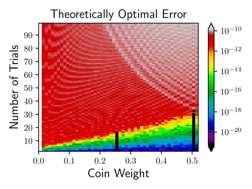
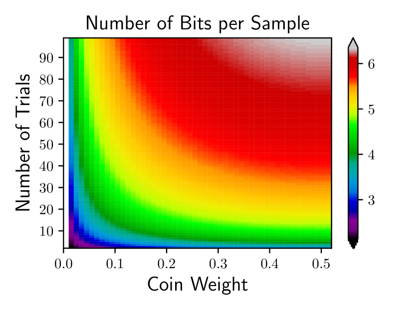
(a) Binomial

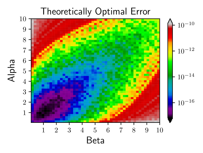
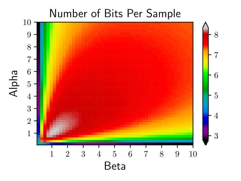
(b) Beta Binomial $(n\,{=}\,80)$

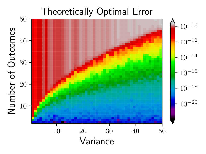
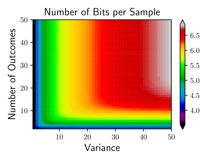
(c) Discrete Gaussian

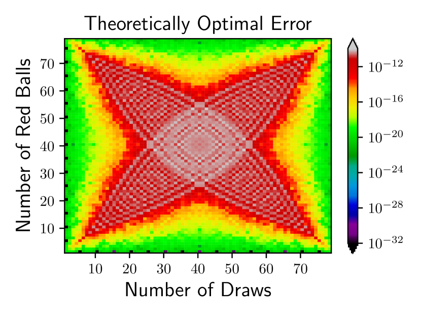
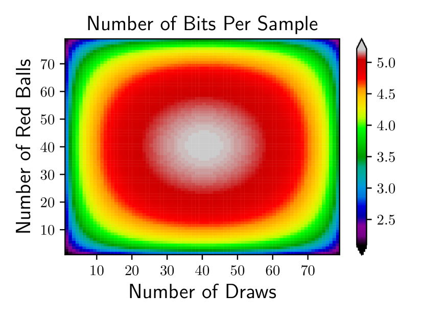
(d) Hypergeometric $(n\,{=}\,80)$

Figure 2. Characterization of the theoretically optimal approximation error (top row) and average number of bits per sample (bottom row) for four common families of probability distributions using $k=32$ bits of precision.

Figure 2 shows how the closest-approximation error (top row) and entropy consumption (bottom row) vary with two of the parameters of each family (x and y-axes) when using $k=32$ bits of precision. Since Beta Binomial and Hypergeometric have three parameters, we fix $n=80$ and vary the remaining two parameters. Closest-approximation distributions are obtained from Algorithm 3, using $Z=2^{32}$ and the Hellinger divergence (which is most sensitive at medium entropies). The plots show that, even with the same family, the closest-approximation error is highly dependent on the target distribution and the interaction between parameter values. For example, in Figure 2(a) (top panel), the black spikes at coin weight 0.25 and 0.50 correspond to pairs $(n,p)$ where the binomial distribution can be sampled exactly. Moreover, for a fixed coin weight (x-axis), the error increases as the number of trials (y-axis) increases. The rate at which the error increases with the number of trials is inversely proportional to the coin weight, which is mirrored by the fact that the average number of bits per sample (bottom panel) varies over a wider range and at a faster rate at low coin weights than at high coin weights. In Figure 2(c), for a fixed level of variance (x-axis), the error increases until the number of outcomes (y-axis) exceeds the variance, after which the tail probabilities become negligible. In Figure 2(d) when the number of red balls $m$ and number of draws $d$ are equal to roughly half of the population size $n$, the bits per sample and approximation error are highest (grey in center of both panels). This relationship stands in contrast to Figure 2(b), where approximation error is lowest (black/purple in lower left of top panel) when bits per sample is highest (grey in lower left of bottom panel). The methods presented in this paper enable rigorous and systematic assessments of the effects of bit precision on theoretically-optimal entropy consumption and sampling error, as opposed to empirical, simulation-based assessments of entropy and error which can be very noisy in practice (e.g., Jonas (2014, Figure 3.15)).

6.2. Comparing Error, Entropy, and Runtime to Baseline Limited-Precision Algorithms

We next show that the proposed sampling algorithm is more accurate, more entropy-efficient, and faster than existing limited-precision sampling algorithms. We briefly review two baselines below.

Inversion sampling. Recall from Section 1.1 that inversion sampling is a universal method based on the key property in Eq. (1). In the $k$-bit limited-precision setting, a floating-point number $U^{\prime}$ (with denominator $2^{k}$) is used to approximate a real uniform variate $U$. The GNU C++ standard library (Lea, 1992) v5.4.0 implements inversion sampling as in Algorithm 2 (using $\leq$ instead of $<$). As $W\sim\mathsf{Uniform}(\{0,1/2^{k},\dots,(2^{k}-1)/2^{k}\})$, it can be shown that the limited-precision inversion sampler has the following output probabilities $\hat{p}_{i}$, where $\widetilde{p}_{j}\coloneqq\sum_{s=1}^{j}p_{s}$ $(j=1,\dots,n)$ and $2\leq i\leq n$:

(46) $$\hat{p}_{1}\propto\lfloor 2^{k}\widetilde{p}_{1}\rfloor+\mathbf{1}_{\widetilde{p}_{1}\neq 1}; \hat{p}_{i}\propto\begin{cases}\max(0,\lceil 2^{k}\widetilde{p}_{i}\rceil-\lfloor 2^{k}\widetilde{p}_{i-1}\rfloor)&(\mbox{if }2^{k}\widetilde{p}_{i}=\lfloor 2^{k}\widetilde{p}_{i}\rfloor\mbox{ and }\widetilde{p}_{i}\neq 1)\\ \max(0,\lceil 2^{k}\widetilde{p}_{i}\rceil-\lfloor 2^{k}\widetilde{p}_{i-1}\rfloor-1)&(\mbox{otherwise})\end{cases}.$$

Interval algorithm (Han and Hoshi, 1997). This method implements inversion sampling by recursively partitioning the unit interval $[0,1]$ and using the cumulative distribution of $\mathbf{p}$ to lazily find the bin in which a uniform random variable falls. We refer to Uyematsu and Li (2003, Algorithm 1) for a limited-precision implementation of the interval algorithm using $k$-bit integer arithmetic.

Table 2. Comparison of the average number of input bits per sample used by inversion sampling, interval sampling, and the proposed method, in each of the six parameterized families using $k\,{=}\,16$ bits of precision.

Distribution	Average Number of Bits per Sample
	Inversion Sampler (Alg. 2)	Interval Sampler (Uyematsu and Li, 2003)	Optimal Sampler (Alg. 7)
Benford	16	6.34	5.71
Beta Binomial	16	4.71	4.16
Binomial	16	5.05	4.31
Boltzmann	16	1.51	1.03
Discrete Gaussian	16	6.00	5.14
Hypergeometric	16	4.04	3.39

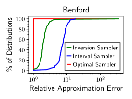
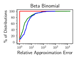
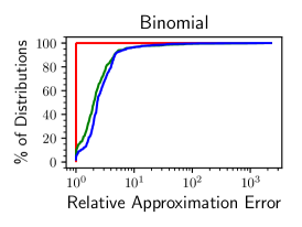
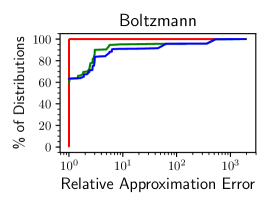
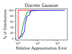
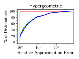
Figure 3. Comparison of the approximation error of limited-precision implementations of interval sampling (green) and inversion sampling (blue) relative to error obtained by the optimal sampler (red), for six families of probability distributions using $k\,{=}\,16$ of bits precision. The x-axis shows the approximation error of each sampler relative to the optimal error. The y-axis shows the fraction of 500 distributions from each family whose relative error is less than or equal to the corresponding value on the x-axis.

6.2.1. Error Comparison

Both the inversion and interval samplers use at most $k$ bits of precision, which, from Proposition 2.16, means that these algorithms are less accurate than the optimal approximate samplers from Algorithm 3 (using $Z=2^{k}$) and less entropy-efficient than the sampler in Algorithm 7. To compare the errors, 500 distributions are obtained by sweeping through a grid of values that parameterize the shape and dimension for each of six families of probability distributions. For each target distribution, probabilities from the inversion method (from Eq. (46)), the interval method (computed by enumeration), and the optimal approximation (from Algorithm 3) are obtained using $k=16$ bits of precision. In Figure 3, the x-axis shows the approximation error (using the Hellinger divergence) of each method relative to the theoretically-optimal error achieved by our samplers. The y-axis shows the fraction of the 500 distributions whose relative error is less than or equal to the value on the x-axis. The results show that, for this benchmark set, the output distributions of inversion and interval samplers are up to three orders of magnitude less accurate relative to the output distribution of the optimal $k$-bit approximation delivered by our algorithm.

6.2.2. Entropy Comparison

Next, we compare the efficiency of each sampler measured in terms of the average number of random bits drawn from the source to produce a sample, shown in Table 2. Since these algorithms are guaranteed to halt after consuming at most $k$ random bits, the average number of bits per sample is computed by enumerating over all $2^{k}$ possible $k$-bit strings (using $k=16$ gives 65536 possible input sequences from the random source) and recording, for each sequence of input bits, the number of consumed bits until the sampler halts. The inversion algorithm consumes all $k$ available bits of entropy, unlike the interval and optimal samplers, which lazily draw bits from the random source until an outcome can be determined. For all distributional families, the optimal sampler uses fewer bits per sample than are used by interval sampling.

Figure 4. Comparison of wall-clock time per sample and order of growth of two implementations of the optimal samplers (using Algorithms 7 and 8) with inversion sampling (using linear and binary search in Algorithm 2).

Table 3. Comparison of runtime and number of calls to the random number generator using limited-precision entropy-optimal and inversion sampling to generate $100$ million samples from $100$ dimensional distributions

Method	Entropy of Target Distribution	Number of PRNG Calls	PRNG Wall-Clock Time (ms)
Optimal Approximate Sampler (Alg. 7)	0.5	7,637,155	120
	2.5	11,373,471	160
	4.5	18,879,900	260
	6.5	24,741,348	350
Inversion Sampler (Alg. 2)	(all)	100,000,000	1410

6.2.3. Runtime Comparison

We next assess the runtime performance of our sampling algorithms as the dimension and entropy of the target distribution increases. For each $n\in\{10,100,1000,10000\}$, we generate 1000 distributions with entropies ranging from $0,\dots,\log(n)$. For each distribution, we measure the time taken to generate a sample based on 100000 simulations according to four methods: the optimal sampler using SampleEncoding (Algorithm 7); the optimal sampler using SampleMatrix (Algorithm 8); the inversion sampler using a linear scan (Algorithm 2, as in the GNU C++ standard library); and the inversion sampler using binary search (fast C implementation). Figure 4 shows the results, where the x-axis is the entropy of the target distribution and the y-axis is seconds per sample (log scale). In general, the difference between the samplers increases with the dimension $n$ of the target distribution. For $n=10$, the SampleEncoding sampler executes a median of over 1.5x faster than any other sampler. For $n=10000$, SampleEncoding executes a median of over 3.4x faster than inversion sampling with binary search and over 195x faster than the linear inversion sampler implemented in the C++ library. In comparison with SampleMatrix (Roy et al., 2013), SampleEncoding is faster by a median of 2.3x ($n=10$) to over 5000x ($n=10000$).

The worst runtime scaling is given by SampleMatrix which, although entropy-optimal, grows order $nH(\mathbf{p})$ due to the inner loop through the rows of the probability matrix. In contrast, SampleEncoding uses the dense linear array described in Section 5 and is asymptotically more efficient: its runtime depends only on the entropy $H(\mathbf{p})\leq\log{n}$. As for the inversion methods, there is a significant gap between the runtime of SampleEncoding (orange) and the binary inversion sampler (red) at low values of entropy, which is especially visible at $n=1000$ and $n=10000$. The binary inversion sampler scales order $\log{n}$ independently of the entropy, and is thus less performant than SampleEncoding when $H(\mathbf{p})\ll\log{n}$ (the gap narrows as $H(\mathbf{p})$ approaches $\log{n}$).

Table 3 shows the wall-clock improvements from using Algorithm 7. Floating-point sampling algorithms implemented in standard software libraries typically make one call to the pseudorandom number generator per sample, consuming a full 32-bit or 64-bit pseudorandom word, which in general is highly wasteful. (As a conceptual example, sampling $\textsf{Bernoulli}(1/2)$ requires sampling only one random bit, but comparing an approximately-uniform floating-point number $U^{\prime}<0.5$ as in inversion sampling uses e.g., 64 bits.) In contrast, the optimal approximate sampler (Algorithm 7) is designed to lazily consume random bits (following Lumbroso (2013), our implementation of $\mathsf{flip}$ stores a buffer of pseudorandom bits equal to the word size of the machine) which results in fewer function calls to the underlying pseudorandom number generator and 4x–12x less wall-clock time.

Table 4. Precision, entropy consumption, and sampling error of Knuth and Yao sampling, rejection sampling, and optimal approximate sampling, at various levels of precision for the $\textsf{Binomial}(50,61/500)$ distribution.

Method	Precision $k_{(l)}$	Bits per Sample	Error ($L_{1}$)
Exact Knuth and Yao Sampler (Thm. 2.9)	$$5.6\text{\times}{10}^{104}$_{(100)}$	5.24	0.0
Exact Rejection Sampler (Alg. 1)	$449_{(448)}$	735	0.0
Optimal Approximate Sampler (Alg. 3+7)	$4_{(4)}$	5.03	$2.03\text{\times}{10}^{-01}$
	$8_{(4)}$	5.22	$1.59\text{\times}{10}^{-02}$
	$16_{(0)}$	5.24	$6.33\text{\times}{10}^{-05}$
	$32_{(12)}$	5.24	$1.21\text{\times}{10}^{-09}$
	$64_{(29)}$	5.24	$6.47\text{\times}{10}^{-19}$

6.3. Comparing Precision, Entropy, and Error to Exact Sampling Algorithms

Recall that two algorithms for sampling from $Z$-type distributions (Definition 4.3) are: (i) exact Knuth and Yao sampling (Theorem 2.9), which samples from any $Z$-type distribution using at most $H(\mathbf{p})+2$ bits per sample and precision $k$ described in Theorem 3.4; and (ii) rejection sampling (Algorithm 1), which samples from any $Z$-type distribution using $k$ bits of precision (where $2^{k-1}<Z\leq 2^{k}$) using $k2^{k}/Z$ bits per sample. Consider the $\textsf{Binomial}(50,61/500)$ distribution $\mathbf{p}$, which is the number of heads in 50 tosses of a biased coin whose probability of heads is $61/500$. The probabilities are $p_{i}\coloneqq\binom{50}{i}\left({61}/{500}\right)^{i}\left({39}/{500}\right)^{n-i}$ $(i=0,\dots,n)$ and $\mathbf{p}$ is a $Z$-type distribution with $Z=$8.881\,784\,197\,001\,252\,323\,389\,053\,344\,726\,562\,5\text{\times}{10}^{134}$$. Table 4 shows a comparison of the two exact samplers to our optimal approximate samplers. The first column shows the precision $k_{(l)}$, which indicates $k$ bits are used and $l$ (where $0\leq l\leq k$) is the length of the repeating suffix in the number system $\mathbb{B}_{kl}$ (Section 3). Recall that exact samplers use finite but arbitrarily high precision. The second and third columns show bits per sample and sampling error, respectively.

Exact Knuth and Yao sampler. This method requires a tremendous amount of precision to generate an exact sample (following Theorem 3.5), as dictated by the large value of $Z$ for the $\textsf{Binomial}(50,61/500)$ distribution. The required precision far exceeds the amount of memory available on modern machines. Although at most 5.24 bits per sample are needed on average (two more than the 3.24 bits of entropy in the target distribution), the DDG tree has more than ${10}^{104}$ levels. Assuming that each level is a byte, storing the sampler would require around ${10}^{91}$ terabytes.

Exact rejection sampler. This method requires $449$ bits of precision (roughly 56 bytes), which is the number of bits needed to encode common denominator $Z$. This substantial reduction in precision as compared to the Knuth and Yao sampler comes at the cost of higher number of bits per sample, which is roughly 150x higher than the information-theoretically optimal rate. The higher number of expected bits per sample leads to wasted computation and higher runtime in practice due to excessive calls to the random number generator (as illustrated in Table 3).

Optimal approximate sampler. For precision levels ranging from $k=4$ to $64$, the selected value of $l$ delivers the smallest approximation error across executions of Algorithm 3 on inputs $Z_{kk},\dots,Z_{k0}$. At each precision, the number of bits per sample has an upper bound that is very close to the upper bound of the optimal rate, since the entropies of the closest-approximation distributions are very close to the entropy of the target distribution, even at low precision. Under the $L_{1}$ metric, the approximation error decreases exponentially quickly with the increase in precision (Theorem 4.17).

These results illustrate that exact Knuth and Yao sampling can be infeasible in practice, whereas rejection sampling requires less precision (though higher than what is typically available on low precision sampling devices (Mansinghka and Jonas, 2014)) but is wasteful in terms of bits per sample. The optimal approximate samplers are practical to implement and use significantly less precision or bits per sample than exact samplers, at the expense of a small approximation error that can be controlled based on the accuracy and entropy constraints of the application at hand.

7. Conclusion

This paper has presented a new class of algorithms for optimal approximate sampling from discrete probability distributions. The samplers minimize both statistical error and entropy consumption among the class of all entropy-optimal samplers and bounded-entropy samplers that operate within the given precision constraints. Our samplers lead to improvements in accuracy, entropy-efficiency, and wall-clock runtime as compared to existing limited-precision samplers, and can use significantly fewer computational resources than are needed by exact samplers.

Many existing programming languages and systems include libraries and constructs for random sampling (Lea, 1992; MathWorks, 1993; R Core Team, 2014; Galassi et al., 2019). In addition to the areas of scientific computing mentioned in Section 1, relatively new and prominent directions in the field of computing that leverage random sampling include probabilistic programming languages and systems (Gordon et al., 2014; Saad and Mansinghka, 2016; Staton et al., 2016; Cusumano-Towner et al., 2019); probabilistic program synthesis (Nori et al., 2015; Saad et al., 2019); and probabilistic hardware (de Schryver et al., 2012; Dwarakanath and Galbraith, 2014; Mansinghka and Jonas, 2014). In all these settings, the efficiency and accuracy of random sampling procedures play a key role in many implementation techniques. As uncertainty continues to play an increasingly prominent role in a range of computations and as programming languages move towards more support for random sampling as one way of dealing with this uncertainty, trade-offs between entropy consumption, sampling accuracy, numerical precision, and wall-clock runtime will form an important set of design considerations for sampling procedures. Due to their theoretical optimality properties, ease-of-implementation, and applicability to a broad set of statistical error measures, the algorithms in this paper are a step toward a systematic and practical approach for navigating these trade-offs.

Appendix A Optimal approximation error at various levels of bit precision

We study how the theoretically-optimal approximation error realized by our samplers (using Algorithm 3) varies with the entropy of the target distribution $\mathbf{p}$ and the number of bits of precision $k$ available to the sampling algorithm. We obtain 10000 probability distributions $\{\mathbf{p}_{1},\dots,\mathbf{p}_{10000}\}$ over $n=100$ dimensions with entropies ranging from $0$ (deterministic distribution) to $\log(100)\,{\approx}\,6.6$ (uniform distribution). For each $\mathbf{p}_{i}$ $(i=1,\dots,10000)$ and precision values $k=1,\dots,20$, we obtain an optimal approximation $\hat{\mathbf{p}}_{ik}$ using Algorithm 3 with $Z=2^{k}$ and measure the approximation error $\Delta_{ik}\coloneqq\Delta(\mathbf{p}_{i},\mathbf{p}_{ik})$. Figure 5 shows a heatmap of the approximation errors $\Delta_{ik}$ according to three common $f$-divergences: total variation, Hellinger divergence, and relative entropy, which are defined in Table 1. Under the relative entropy divergence, all approximation errors are infinite whenever the precision $k<7$ (white area; Figure 5(c)), since the sampler needs at least 7 bits of precision to assign a non-zero probability to each of the $n=100$ outcomes of the target distributions.

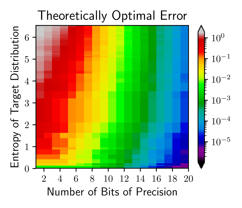
(a) Total Variation

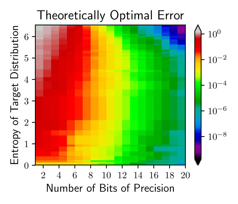
(b) Hellinger Divergence

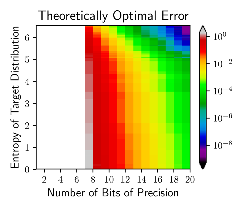
(c) Relative Entropy

Figure 5. Characterization of theoretically optimal approximation errors according to three $f$-divergences (total variation, Hellinger, and relative entropy) for target distributions over $n\,{=}\,100$ dimensions.

In all three plots, for a fixed level of entropy (y-axis), the approximation error tends to zero as the precision increases from $k=1$ to $k=20$ (x-axis). However, the relationship between approximation error and entropy of the target distribution under each divergence. For total variation, the approximation error increases as the entropy increases at both low-precision values (gray area; top-left of Figure 5(a)) and high-precision values (purple area; bottom-right of Figure 5(a)). In contrast, for relative entropy, the approximation error decreases as the entropy increases at both low-precision values (gray area; bottom-center-left of Figure 5(a)) and high-precision values (purple area; top-right of Figure 5(a)). For the Hellinger divergence, the approximation error contains both of these characteristics; more specifically, it behaves like the error under total variation at low precision (gray area; top-left of Figure 5(b)) and like the error under relative entropy at high precision (purple area; top-right of Figure 5(b)). More generally, the distributions with highest approximation error under the Hellinger divergence lie in the center of the entropy values and the distributions with the lowest approximations lie at the low and high end of the entropy values.

These studies provide systematic guidelines for obtaining theoretically-minimal errors of entropy-optimal approximate samplers according to various $f$-divergences in applications where precision and accuracy are key design considerations. For example, Jonas (2014) empirically measure the effects of bit precision (using 4 to 12 bits) on the sampling error (measured by the relative entropy) of a 1000-dimensional multinomial hardware gate. In cryptographic applications, a common requirement for various security guarantees is to sample from a discrete Gaussian lattice with an approximation error (measured by total variation) of at most $2^{-90}$ (Dwarakanath and Galbraith, 2014), and various limited-precision samplers aim to operate within these bounds (Folláth, 2014).

Appendix B Deferred Proofs

This section proves Theorem 4.17 from the main text, which is restated below.

Theorem B.1.

If $\Delta_{g}$ is the total variation divergence, then any optimal solution $\mathbf{M}$ returned by Algorithm 3 satisfies $\Delta_{g}(\mathbf{p},\mathbf{M})\leq n/2Z$.

We begin by first establishing the following result.

Theorem B.2.

Let $\mathbf{p}\coloneqq(p_{1},\dots,p_{n})$ be a probability distribution, $Z>0$ an integer, and $\Delta_{g}$ be total variation divergence. Any assignment $\mathbf{M}\in\mathcal{M}[n,Z]$ that minimizes $\Delta_{g}(\mathbf{p},\mathbf{M})$ satisfies:

(47) $$\lfloor Z{p_{i}}\rfloor\leq M_{i}\leq\lfloor Z{p_{i}}\rfloor+1 (i=1,\dots,n).$$

Proof.

Write $\chi(w)\coloneqq w-\lfloor w\rfloor$ to denote the fractional part of a real number $w$. From the correspondence of the total variation to the $L_{1}$ distance, the objective function may be rewritten as

(48) $$\Delta_{g}(\mathbf{p},\mathbf{M})=\frac{1}{2}\sum_{i=1}^{n}\left\lvert M_{i}/Z-p_{i}\right\rvert.$$

Optimizing $\Delta_{g}(\mathbf{p},\cdot)$ is equivalent to optimizing $\Delta^{\prime}_{g}(\mathbf{p},\cdot)$, defined by

(49) $$\Delta^{\prime}_{g}(\mathbf{p},\mathbf{M})\coloneqq 2Z\Delta_{g}(\mathbf{p},\mathbf{M})=\sum_{i=1}^{n}\left\lvert M_{i}-Z{p_{i}}\right\rvert.$$

Let $\mathbf{M}$ be any assignment that minimizes $\Delta^{\prime}_{g}(\mathbf{p},\cdot)$. We will show the upper bound and lower bound in (47) separately.

(Upper bound)

Assume toward a contradiction that there is some $t\in[n]$ such that $M_{t}=\lfloor Z{p_{t}}\rfloor+c$ for some integer $c>1$.

We first claim that there must be some $j\neq t$ such that $M_{j}<Z{p_{j}}$. Assume not. Then $Z{p_{i}}\leq M_{i}$ for all $i\in[n]$, which gives

(50) $$\sum_{i=1}^{n}M_{i}\geq\sum_{\begin{subarray}{c}i=1\\ i\neq t\end{subarray}}^{n}Z{p_{i}}+\lfloor Z{p_{t}}\rfloor+c =\sum_{\begin{subarray}{c}i=1\\ i\neq t\end{subarray}}^{n}Z{p_{i}}+\lfloor Z{p_{t}}\rfloor+c$$

(51) $$=\sum_{\begin{subarray}{c}i=1\\ i\neq t\end{subarray}}^{n}Z{p_{i}}+Z{p_{t}}-\chi(Z{p_{i}t})+c$$

(52) $$=\sum_{i=1}^{n}Z{p_{t}}+(c-\chi(Z{p_{t}}))=Z+(c-\chi(Z{p_{t}}))>Z,$$

where the final inequality follows from $c>1>\chi(Z{p_{t}})$. But (52) contradicts $\mathbf{M}\in\mathcal{M}[n,Z]$.

Consider the assignment $\mathbf{W}\coloneqq(W_{1},\dots,W_{n})\in\mathcal{M}[n,Z]$ defined by

(53) $$W_{i}\coloneqq\begin{cases}M_{i}-1&\mbox{if~{}}i=t,\\ M_{i}+1&\mbox{if~{}}i=j,\\ M_{i}&\mbox{otherwise}.\end{cases} (i=1,\dots,n)$$

We will establish that $\Delta^{\prime}_{g}(\mathbf{p},\mathbf{W})<\Delta^{\prime}_{g}(\mathbf{p},\mathbf{M})$, contradicting the optimality of $\mathbf{M}$. From cancellation of like-terms, we have

(54) $$\Delta^{\prime}_{g}(\mathbf{p},\mathbf{W})-\Delta^{\prime}_{g}(\mathbf{p},\mathbf{M})=\left[\lvert W_{t}-Z{p_{t}}\rvert-\lvert M_{t}-Z{p_{t}}\rvert\right]+\left[\lvert W_{j}-Z{p_{j}}\rvert-\lvert M_{j}-Z{p_{j}}\rvert\right].$$

For the first term in the right-hand side of (54), we have

(55) $$\lvert W_{t}-Z{p_{t}}\rvert-\lvert M_{t}-Z{p_{t}}\rvert=(M_{t}-1-Z{p_{t}})-(M_{t}-Z)=-1,$$

where the first equality uses the fact that $c\geq 2$, so that

(56) $$W_{t}=M_{t}-1=\lfloor Z{p_{t}}\rfloor+c-1\geq\lfloor Z{p_{t}}\rfloor+1>Z{p_{t}}.$$

We now consider the second term of (54), and proceed by cases.

1. $M_{j}<\lfloor Z{p_{j}}\rfloor$. Then clearly

   (57) $$\lvert W_{j}-Z{p_{j}}\rvert-\lvert M_{j}-Z{p_{j}}\rvert=(Z{p_{j}}-(M_{j}+1))-(Z{p_{j}}-M_{j})=-1.$$

2. $M_{j}=\lfloor Z{p_{j}}\rfloor$. Since $M_{j}<Z{p_{j}}$, we have $\lfloor Z{p_{j}}\rfloor<Z{p_{j}}$ and $0<\chi(Z{p_{j}})<1$, which gives

   (58) $$\lvert W_{j}-Z{p_{j}}\rvert-\lvert M_{j}-Z{p_{j}}\rvert =(M_{j}+1-Z{p_{j}})-(Z{p_{j}}-M_{j})$$

   (59) $$=1-2(Z{p_{j}}-M_{j})$$

   (60) $$=1-2\chi(Z{p_{j}})$$

   (61) $$<1.$$

Combining (57) and (61) from these two cases gives the upper bound

(62) $$\lvert W_{j}-Z{p_{j}}\rvert-\lvert M_{j}-Z{p_{j}}\rvert<1.$$

Using (57) and (62) in (54), we obtain

(63) $$\Delta^{\prime}_{g}(\mathbf{p},\mathbf{W})-\Delta^{\prime}_{g}(\mathbf{p},\mathbf{M}) =\left[\lvert W_{t}-Z{p_{t}}\rvert-\lvert M_{t}-Z{p_{t}}\rvert\right]+\left[\lvert W_{j}-Z{p_{j}}\rvert-\lvert M_{j}-Z{p_{j}}\rvert\right]$$

(64) $$<-1+1=0,$$

establishing a contradiction to the optimality of $\mathbf{M}$.

(Lower Bound)

Assume toward a contradiction that there exists $t\in[n]$ such that $M_{t}<\lfloor Z{p_{t}}\rfloor$.

We first claim that there must exist $j\neq t$ such that $Z{p_{j}}<M_{j}$. Assume not. Then $M_{i}\leq Z{p_{i}}$ for all $i\in[n]$, which gives

(65) $$\sum_{i=1}^{n}M_{i}<\sum_{\begin{subarray}{c}i=1\\ i\neq t\end{subarray}}^{n}Z{p_{i}}+\lfloor Z{p_{t}}\rfloor\leq\sum_{\begin{subarray}{c}i=1\\ i\neq t\end{subarray}}^{n}Z{p_{i}}+Z{p_{t}}=Z,$$

which again contradicts $\mathbf{M}\in\mathcal{M}[n,Z]$.

The remainder of the proof is symmetric to that of the upper bound, where the assignment $\mathbf{W}\in\mathcal{M}[n,Z]$ defined by

(66) $$W_{i}\coloneqq\begin{cases}M_{i}+1&\mbox{if~{}}i=t,\\ M_{i}-1&\mbox{if~{}}i=j,\\ M_{i}&\mbox{otherwise}\end{cases} (i=1,\dots,n)$$

can be shown to satisfy $\Delta^{\prime}_{g}(\mathbf{p},\mathbf{W})<\Delta^{\prime}_{g}(\mathbf{p},\mathbf{M})$, contradicting the optimality of $\mathbf{M}$. ∎

Proof of Theorem B.1.

From Theorem B.2, we have

(67) $$\lfloor Z{p_{i}}\rfloor\leq M_{i}\leq\lfloor Z{p_{i}}\rfloor+1\implies\lvert M_{i}-Z{p_{i}}\rvert\leq 1\implies\lvert M_{i}/Z-p_{i}\rvert\leq 1/Z (i=1,\dots,n),$$

which along with (48) yields $\Delta_{g}(\mathbf{p},\mathbf{M})\leq n/2Z$. ∎