A deep-learning based Bayesian approach to seismic imaging and uncertainty quantification

Abstract

Uncertainty quantification is essential when dealing with ill-conditioned inverse problems due to the inherent nonuniqueness of the solution. Bayesian approaches allow us to determine how likely an estimation of the unknown parameters is via formulating the posterior distribution. Unfortunately, it is often not possible to formulate a prior distribution that precisely encodes our prior knowledge about the unknown. Furthermore, adherence to handcrafted priors may greatly bias the outcome of the Bayesian analysis. To address this issue, we propose to use the functional form of a randomly initialized convolutional neural network as an implicit structured prior, which is shown to promote natural images and excludes images with unnatural noise. In order to incorporate the model uncertainty into the final estimate, we sample the posterior distribution using stochastic gradient Langevin dynamics and perform Bayesian model averaging on the obtained samples. Our synthetic numerical experiment verifies that deep priors combined with Bayesian model averaging are able to partially circumvent imaging artifacts and reduce the risk of overfitting in the presence of extreme noise. Finally, we present pointwise variance of the estimates as a measure of uncertainty, which coincides with regions that are more difficult to image.

1 Introduction

Seismic imaging involves an inconsistent, ill-conditioned linear inverse problem due to presence of shadow zones and complex structures in the subsurface, coherent linearization errors, and noisy measured data. As a result, there is uncertainty in the recovered unknown parameters. However, due to the computational complexity of current approaches to uncertainty quantification in seismic inversion [1], most efforts are only focused on computing a maximum a posterior (MAP) estimate. In this work, we propose using Bayesian-inference, which provides a principled way of incorporating uncertainty into the inversion by generating an ensemble of models that each are a solution to the imaging problem—i.e., sampling the posterior distribution. The choice of prior in a Bayesian framework is crucial and affects the final estimate. Conventional methods mostly rely on handcrafted and unrealistic priors, such as a Gaussian or Laplace distribution prior on the model parameters in the physical or in a transform domain. However, handcrafted priors tend to bias the outcome of the inversion, something we would like to avoid. To address this issue, motivated by earlier attempts in machine learning and geophysics [2, 3, 4], we propose to replace handcrafted priors with an implicit deep prior— i.e., reparameterize the unknown with a randomly initialized deep convolutional neural network (CNN), which is shown to act as a structured prior that promotes natural images, but not unnatural noise. To reduce the risk of overfitting the noise in the data, we perform Bayesian model averaging by sampling the posterior using stochastic gradient Langevin dynamics [SGLD, 5]. Additionally, using the obtained samples from the posterior, we compute pointwise variance of the estimates as a measure of uncertainty.

In addition to numerous efforts to incorporate ideas from deep learning into seismic processing and inversion [6, 7], in the context of Bayesian seismic inversion, there has been relatively few attempts concerning uncertainty qualification. Mosser et al. [8] first train a Generative Adversarial Network on synthetic geological structures. Next, the generator is deployed as an implicit prior in seismic waveform inversion. Finally, these authors run a variant of SGLD on the latent variable of the generative model to sample the posterior and quantify the uncertainty. On the contrary, Herrmann et al. [9] propose a new formulation in the context of seismic imaging that does not require a pretrained generative model. This scheme is based on the Expectation-Maximization method, where they jointly solve the inverse problem and train a generative model capable of directly sampling the posterior. The main distinction of their work is fast posterior sampling since it only requires feed-forward evaluation of the generative model once the joint inversion and training is finished.

First, we mathematically formulate the posterior distribution by introducing the likelihood function and prior distribution involving the deep prior. Next, we discuss our approach to obtain samples from the posterior. Finally, we showcase our method using a synthetic example in the presence of extreme noise.

2 A Bayesian approach to seismic imaging

In seismic imaging, the goal is to estimate the short-wavelength structure of the subsurface, denoted by $\delta\mathbf{m}$, given a smooth background squared-slowness model, $\mathbf{m}_{0}$, observed data, $\mathbf{d}_{i}$, and source signatures, $\mathbf{q}_{i}$, where $i=1,2,\cdots,N$ and $N$ is the number of source experiments. Below we introduce the the likelihood function and prior distribution in our Bayesian framework.

2.1 Likelihood function

We impose a multivariate Gaussian distribution, with a diagonal covariance matrix, on the noise. If $\mathbf{d}_{i}$ is $D$ dimensional, we can write the negative log-likelihood of the observed data as follows:

$$\ -\log p_{\text{noise}}\left(\left\{\mathbf{d}_{i},\mathbf{q}_{i}\right\}_{i=1}^{N}\big{|}\ \delta\mathbf{m}\right)=-\sum_{i=1}^{N}\log p_{\text{noise}}\left(\mathbf{d}_{i},\mathbf{q}_{i}\big{|}\ \delta\mathbf{m}\right)$$ (1)

$$\ =\frac{1}{2\sigma^{2}}\sum_{i=1}^{N}\|\delta\mathbf{d}_{i}-\mathbf{J}(\mathbf{m}_{0},\mathbf{q}_{i})\delta\mathbf{m}\|_{2}^{2}+\frac{ND}{2}\log(2\pi\sigma^{2}),\quad\delta\mathbf{d}_{i}=\mathbf{d}_{i}-\mathbf{P}\mathbf{A}(\mathbf{m}_{0})^{-1}\mathbf{q}_{i}.$$

In these expressions, $p_{\text{noise}}$ is the probability density function of the noise, $\sigma^{2}$ is the estimated noise variance, $\delta\mathbf{d}_{i}$ the data residual, $\mathbf{J}$ the linearized Born scattering operator, $\mathbf{A}$ the discretized wave equation, and $\mathbf{P}$ the restriction operator that restricts the wavefield to the location of the receivers.

2.2 Deep prior— a randomly initialized deep CNN

Being a structured prior for natural images, randomly initialized CNNs are utilized in solving several inverse problems [2, 3, 4]. Motivated by their success, we propose to reparameterize the unknown model perturbations, $\delta\mathbf{m}$, by a randomly initialized deep CNN, $\mathbf{g}(\mathbf{z},\mathbf{w})$—i.e., $\delta\mathbf{m}=\mathbf{g}(\mathbf{z},\mathbf{w})$, where $\mathbf{z}\sim\mathrm{N}(\mathbf{0},\mathbf{I})$ is the fixed input to the CNN and $\mathbf{w}$ denotes the unknown CNN weights, consisting of convolutional kernels and biases. We follow Lempitsky et al. [2] for the CNN architecture. We also impose a Gaussian prior on the weights of the CNN—i.e., $\mathbf{w}\sim\mathrm{N}(\mathbf{0},\frac{1}{\lambda^{2}}\mathbf{I})$, where $\lambda$ is a hyperparameter. The seemingly uninformative Gaussian prior on $\mathbf{w}$ induces a structured prior on the output space because of the carefully designed functional form of the CNN. Figure 1 demonstrates the empirical first and second order statistics induced by the deep prior obtained by evaluating the CNN using $5000$ weights sampled from the prior distribution, $p_{\text{prior}}(\mathbf{w})$.

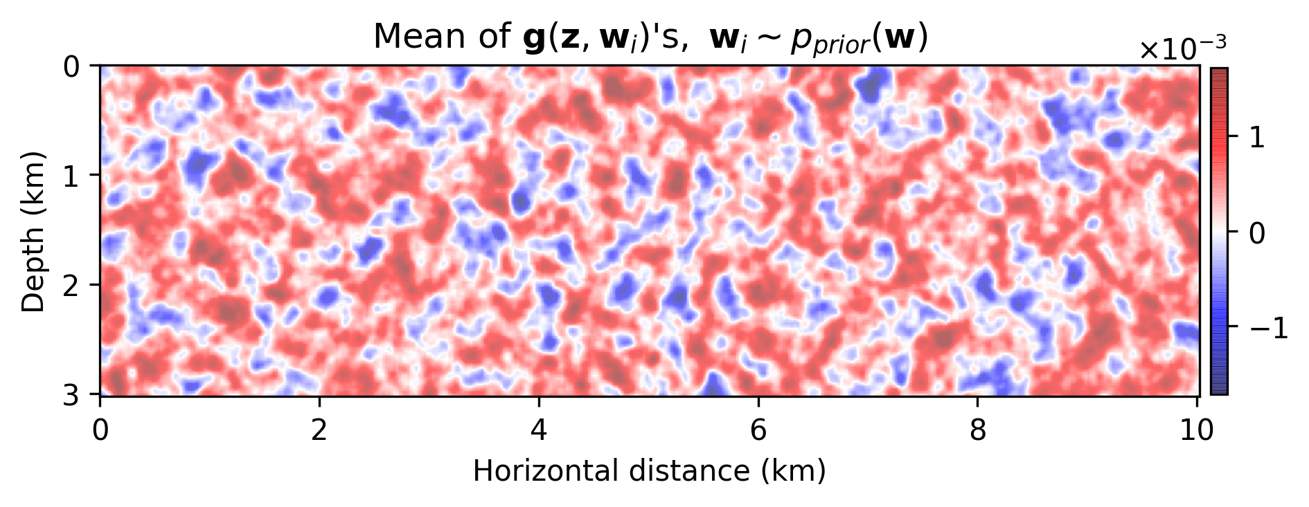
(a)

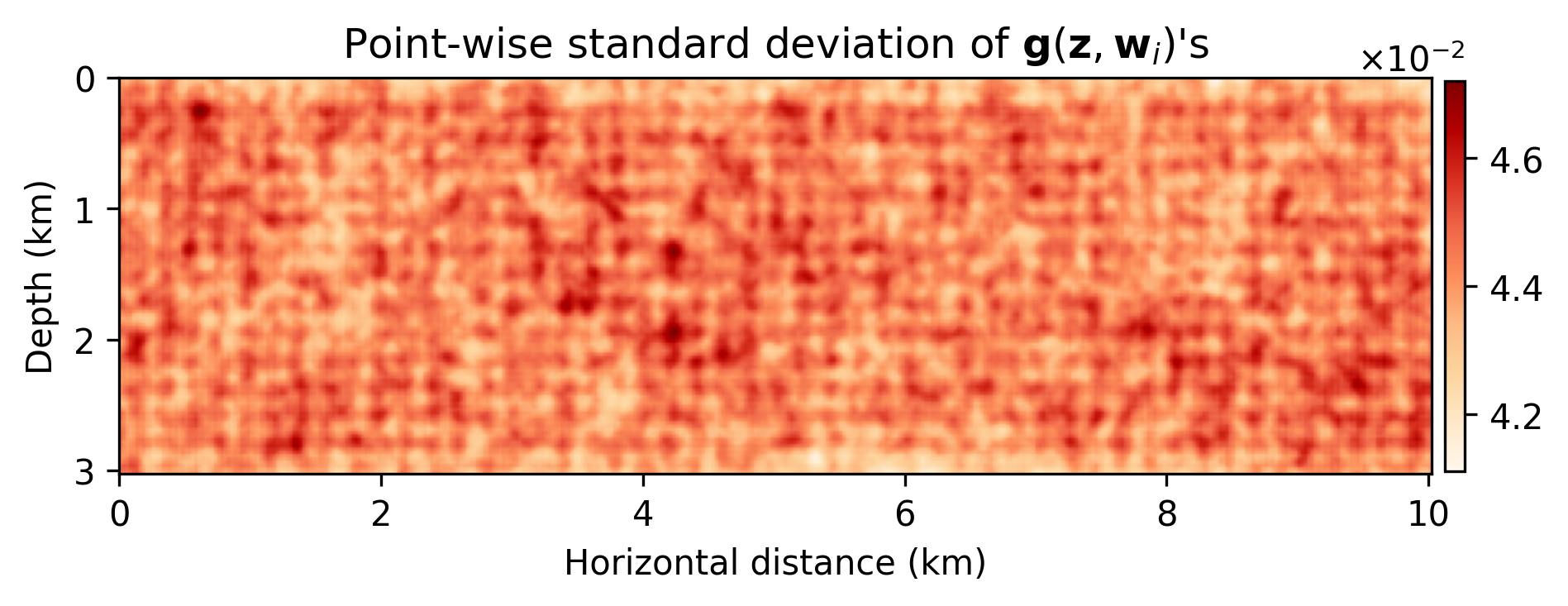
(b)

Figure 1: First and second order statistics of the implicit deep prior. a) The mean of $\mathbf{g}(\mathbf{z},\mathbf{w})$ over $5000$ samples $\mathbf{w}\sim p_{\text{prior}}(\mathbf{w})$. b) The pointwise standard deviation of $\mathbf{g}(\mathbf{z},\mathbf{w})$ over the drawn samples.

Based on the definitions above, we can write the negative log-posterior as follows:

$$-\log p_{\text{post}}\left(\mathbf{w}\big{|}\left\{\mathbf{d}_{i},\mathbf{q}_{i}\right\}_{i=1}^{N},\mathbf{z}\right) \ =-\left[\sum_{i=1}^{N}\log p_{\text{noise}}\left(\mathbf{d}_{i},\mathbf{q}_{i}\big{|}\ \mathbf{w},\mathbf{z}\right)\right]-\log p_{\text{prior}}\left(\mathbf{w}\right)\quad+\underbrace{\text{const}}_{\text{independent of }\mathbf{w}}$$ (2)

$$\ =\frac{1}{2\sigma^{2}}\sum_{i=1}^{N}\|\delta\mathbf{d}_{i}-\mathbf{J}(\mathbf{m}_{0},\mathbf{q}_{i})\mathbf{g}(\mathbf{z},\mathbf{w})\|_{2}^{2}+\frac{\lambda^{2}}{2}\|\mathbf{w}\|_{2}^{2}\quad+\quad\text{const,}$$

where $p_{\text{post}}$ is the posterior distribution. In the next section, we present how we reap information on the posterior distribution, $p_{\text{post}}(\mathbf{w}\big{|}\left\{\mathbf{d}_{i},\mathbf{q}_{i}\right\}_{i=1}^{N},\mathbf{z})$.

2.3 Sampling the posterior— stochastic gradient Langevin dynamics

The minimizer of the negative log-posterior (Equation 2) with respect to $\mathbf{w}$ is the MAP estimate. Sampling the posterior distribution, instead of simply computing the MAP estimate, allows us to incorporate the model uncertainty into the final estimate (Equation 4). While Bayesian inference in deep CNNs is generally intractable, a popular approach to sample the posterior is SGLD [5]. As described in Equation 3, SGLD is a Markov chain Monte Carlo sampler obtained by injecting Gaussian noise to stochastic gradient descent updates—i.e.,

$$\ \mathbf{w}_{k+1}=\mathbf{w}_{k}-\frac{\epsilon}{2}\nabla_{\mathbf{w}}J^{(i)}(\mathbf{w}_{k})+\boldsymbol{\eta}_{k},\quad\boldsymbol{\eta}_{k}\sim\mathrm{N}(\mathbf{0},\epsilon\mathbf{I}),$$ (3)

where $J^{(i)}(\mathbf{w})=\frac{N}{2\sigma^{2}}\|\delta\mathbf{d}_{i}-\mathbf{J}(\mathbf{m}_{0},\mathbf{q}_{i})\mathbf{g}(\mathbf{z},\mathbf{w})\|_{2}^{2}+\frac{\lambda^{2}}{2}\|\mathbf{w}\|_{2}^{2}$ approximates the negative log-posterior (Equation 2) by using the $i^{\text{th}}$ element in the sum. We integrate Devito’s [10] linearized Born scattering operator into the PyTorch [11] deep learning library, thus allowing us to compute the gradients required in Equation 3 with automatic differentiation. Our implementation can be found on GitHub. Finally, we compute the final estimation by Bayesian model averaging as follows:

$$\delta\widehat{\mathbf{m}} \ =\mathbb{E}_{\mathbf{w}\sim p_{\text{post}}(\mathbf{w}\normalsize{|}\left\{\mathbf{d}_{i},\mathbf{q}_{i}\right\}_{i=1}^{N},\mathbf{z})}\left[\mathbf{g}(\mathbf{z},\mathbf{w})\right]=\int p_{\text{post}}(\mathbf{w}\normalsize{|}\left\{\mathbf{d}_{i},\mathbf{q}_{i}\right\}_{i=1}^{N},\mathbf{z})\mathbf{g}(\mathbf{z},\mathbf{w})d\mathbf{w}$$ (4)

$$\ \simeq\frac{1}{T}\sum_{j=1}^{T}\mathbf{g}(\mathbf{z},\widehat{\mathbf{w}}_{j}),\quad\widehat{\mathbf{w}}_{j}\sim p_{\text{post}}(\mathbf{w}\normalsize{|}\left\{\mathbf{d}_{i},\mathbf{q}_{i}\right\}_{i=1}^{N},\mathbf{z}),\ j=1,\ldots,T\,,$$

where $T$ is the number of samples from the posterior distribution and $\widehat{\mathbf{w}}_{j}$’s denote the samples.

3 Numerical experiment

We apply our framework to a synthetic dataset simulated on the $2$D Overthrust model by solving the acoustic wave equation. Our dataset includes $369$ shot records with $369$ receivers separated by $27$ $\mathrm{m}$, $2$ seconds recording time, and a source wavelet with $8$ $\mathrm{Hz}$ central frequency. We add Gaussian noise drawn from $\mathrm{N}(\mathbf{0},2\mathbf{I})$ to shot records. Taking into the account the linearization error, the signal-to-noise ratio of the observed data is $-11.37$ $\mathrm{dB}$. We generate simultaneous source experiments by mixing the shot records according to $369$ normally distributed source encodings. By conducting extensive parameter tuning, we set $\lambda=170$, $\epsilon=0.002$, and we run $10000$ total SGLD iterations. After the first $3000$ burn-in iterations, we select every $50^{\text{th}}$ update of SGLD as a samples from posterior to reduce correlation among samples. We also set $\sigma^{2}=2.24$, which is the summation of the measurement noise variance and a direct estimation of linearization error variance using the ground-truth perturbation model.

The results are included in Figure 2. Figure 2b is the maximum-likelihood estimate (MLE)— i.e., using no prior distribution, obtained by minimizing Equation 1 with respect to $\delta\mathbf{m}$ with stochastic optimization and early stopping to prevent overfitting the noise, Figure 2c offers a comparison to the MAP estimate, computed by minimizing Equation 2, Figure 2d indicates the estimation via the proposed method, $\delta\widehat{\mathbf{m}}$, Figure 2e is the pointwise standard deviation among the samples from the posterior, and Figure 2f overlays the vertical profiles of the pointwise standard deviation onto the ground-truth model. The black lines indicate the horizontal locations for which we plot the standard-deviation profiles (green lines). Figures 2g and 2h show pointwise histograms of prior and posterior distributions at points indicated by blue circles in Figure 2e. We make the following observations. The prior induced by the architecture of the CNN, without any other prior knowledge, has been successful in generating a reasonable image (Figure 2c) compared to the MLE. The final estimate, $\delta\widehat{\mathbf{m}}$, is smoother than the MAP estimate and contains fewer imaging artifacts. Figure 2e indicates that we have the most uncertainty at the location of the reflectors, and it gets slightly larger by depth, close to boundaries and fault zone, which are more difficult to image. Finally, Figures 2g and 2h indicate sharpening of the histogram after Bayesian inference.

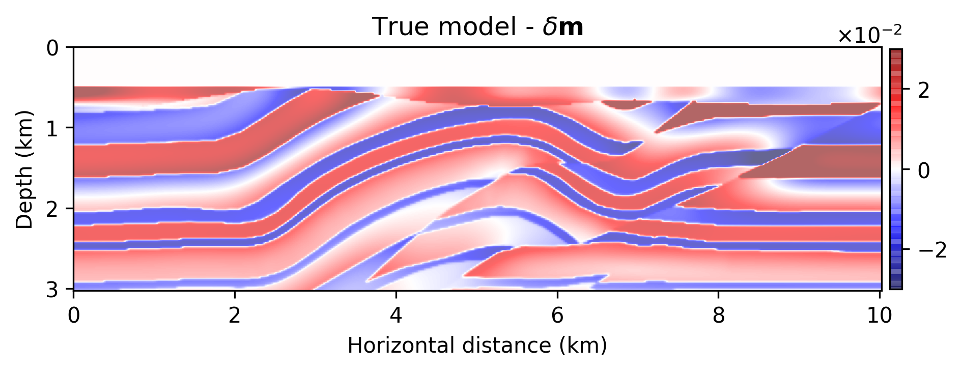
(a)

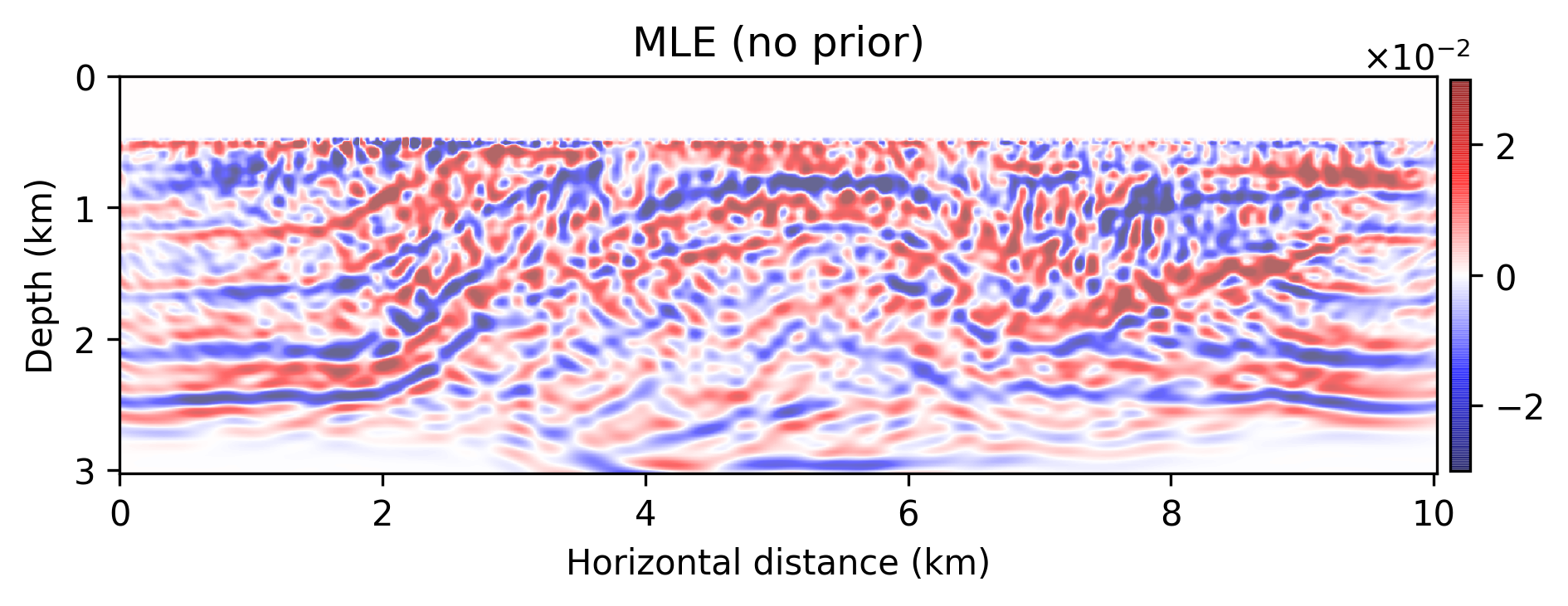
(b)

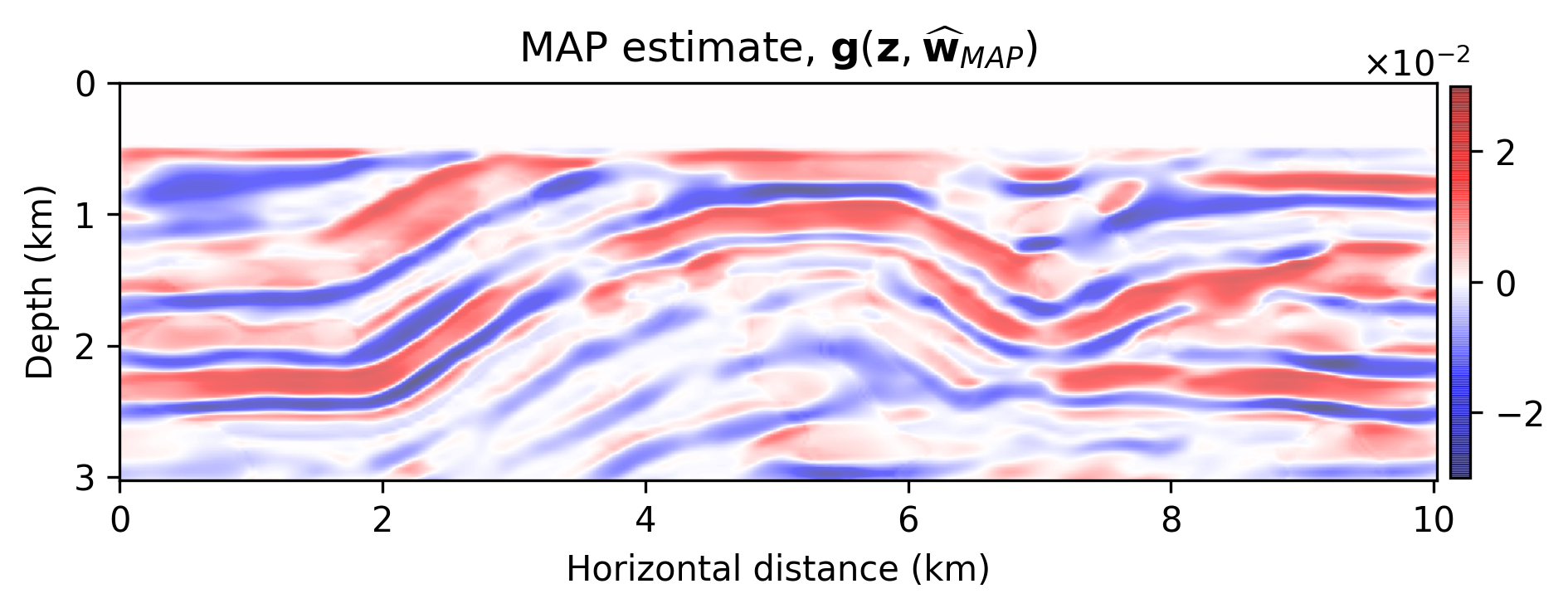
(c)

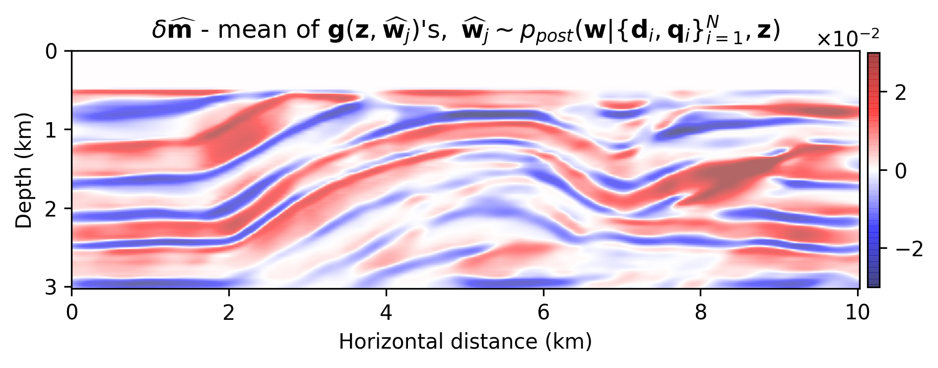
(d)

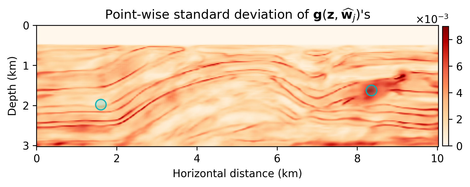
(e)

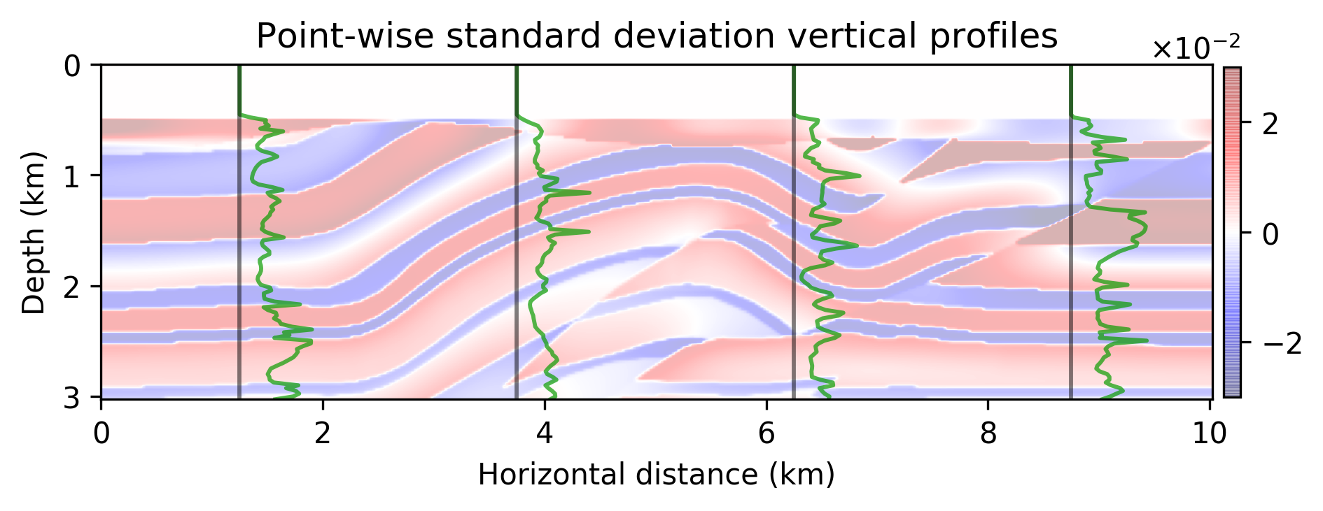
(f)

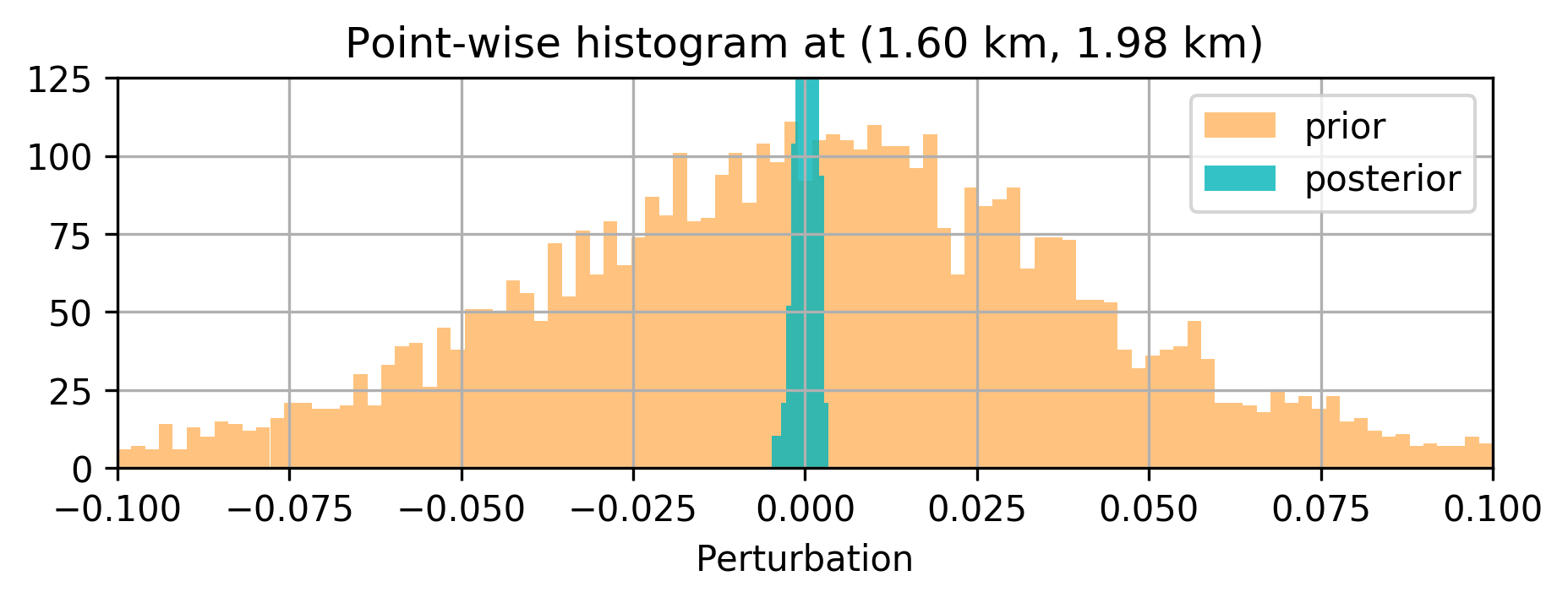
(g)

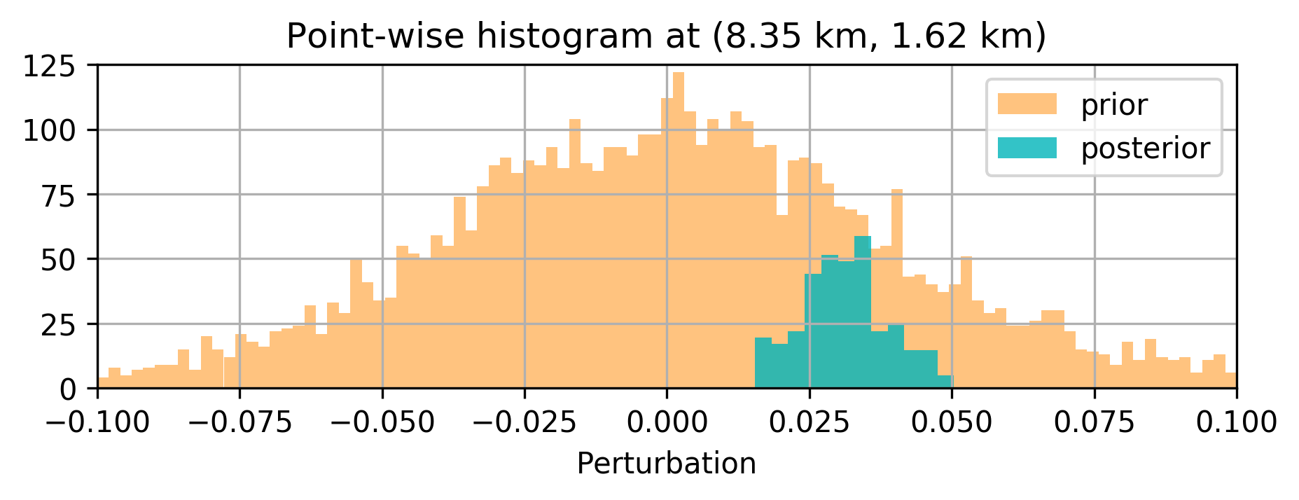
(h)

Figure 2: Imaging and uncertainty quantification. a) True model. b) The MLE —i.e., minimizer of Equation 1 with respect to $\delta\mathbf{m}$. c) The MAP estimate—i.e., minimizer of Equation 2. d) The final estimate, $\delta\widehat{\mathbf{m}}$. e) The pointwise standard deviation among samples drawn from the posterior. f) Standard-deviation profiles. g, h) Point-wise histogram plots at two points in the model indicated by blue dots in Figure 2e.

4 Discussion and conclusions

We introduced a Bayesian framework for seismic imaging that instead of adhering to handcrafted priors utilizes a structured prior induced by a carefully designed convolutional neural network. We demonstrated that our approach is capable of sampling the posterior distribution by running stochastic gradient Langevin dynamics, albeit being expensive, similar to most Markov chain Monte Carlo sampling based approaches. Not withstanding these costs, our formulation is to our knowledge an early attempt to quantify the uncertainty of a convolutional neural network-regularized linear inversion jointly capturing uncertainty in the imaging and the reparametrization with a convolutional neural network. As verified by our numerical experiment, the utilized deep prior was partially able to circumvent the imaging artifacts caused by strong measurement noise and linearization errors. By sampling the posterior and performing Bayesian model averaging, we were able to decrease the artifacts. Finally, the pointwise standard variation plot pointed out more uncertainty at the location of the reflectors, faults, edges, and deeper parts of the model, which coincide with regions that are more difficult to image. As a future direction, we propose to avoid Markov chain Monte Carlo samplers due to their computational complexity.

References

- Fang et al. [2018] Zhilong Fang, Curt Da Silva, Rachel Kuske, and Felix J. Herrmann. Uncertainty quantification for inverse problems with weak partial-differential-equation constraints. GEOPHYSICS, 83(6):R629–R647, 2018. doi: 10.1190/geo2017-0824.1.
- Lempitsky et al. [2018] V. Lempitsky, A. Vedaldi, and D. Ulyanov. Deep Image Prior. In 2018 IEEE/CVF Conference on Computer Vision and Pattern Recognition, pages 9446–9454, June 2018. doi: 10.1109/CVPR.2018.00984.
- Cheng et al. [2019] Zezhou Cheng, Matheus Gadelha, Subhransu Maji, and Daniel Sheldon. A Bayesian Perspective on the Deep Image Prior. In The IEEE Conference on Computer Vision and Pattern Recognition (CVPR), pages 5443–5451, June 2019.
- Wu and McMechan [2019] Yulang Wu and George A McMechan. Parametric convolutional neural network-domain full-waveform inversion. GEOPHYSICS, 84(6):R881–R896, 2019. doi: 10.1190/geo2018-0224.1.
- Welling and Teh [2011] Max Welling and Yee Whye Teh. Bayesian Learning via Stochastic Gradient Langevin Dynamics. In Proceedings of the 28th International Conference on International Conference on Machine Learning, ICML’11, pages 681–688, 2011.
- Siahkoohi et al. [2019] Ali Siahkoohi, Mathias Louboutin, and Felix J. Herrmann. The importance of transfer learning in seismic modeling and imaging. GEOPHYSICS, 84(6):A47–A52, 11 2019. doi: 10.1190/geo2019-0056.1.
- Rizzuti et al. [2019] Gabrio Rizzuti, Ali Siahkoohi, and Felix J. Herrmann. Learned iterative solvers for the Helmholtz equation. 81st EAGE Conference and Exhibition 2019, 2019. ISSN 2214-4609. doi: 10.3997/2214-4609.201901542. URL https://www.slim.eos.ubc.ca/Publications/Private/Submitted/2019/rizzuti2019EAGElis/rizzuti2019EAGElis.pdf.
- Mosser et al. [2019] Lukas Mosser, Olivier Dubrule, and M Blunt. Stochastic Seismic Waveform Inversion Using Generative Adversarial Networks as a Geological Prior. Mathematical Geosciences, 84(1):53–79, 2019. doi: 10.1007/s11004-019-09832-6.
- Herrmann et al. [2019] Felix J. Herrmann, Ali Siahkoohi, and Gabrio Rizzuti. Learned imaging with constraints and uncertainty quantification. In Neural Information Processing Systems (NeurIPS) 2019 Deep Inverse Workshop, 12 2019. URL https://arxiv.org/pdf/1909.06473.pdf.
- Louboutin et al. [2019] M. Louboutin, M. Lange, F. Luporini, N. Kukreja, P. A. Witte, F. J. Herrmann, P. Velesko, and G. J. Gorman. Devito (v3.1.0): an embedded domain-specific language for finite differences and geophysical exploration. Geoscientific Model Development, 12(3):1165–1187, 2019. doi: 10.5194/gmd-12-1165-2019. URL https://www.geosci-model-dev.net/12/1165/2019/.
- Paszke et al. [2019] Adam Paszke, Sam Gross, Francisco Massa, Adam Lerer, James Bradbury, Gregory Chanan, Trevor Killeen, Zeming Lin, Natalia Gimelshein, Luca Antiga, Alban Desmaison, Andreas Kopf, Edward Yang, Zachary DeVito, Martin Raison, Alykhan Tejani, Sasank Chilamkurthy, Benoit Steiner, Lu Fang, Junjie Bai, and Soumith Chintala. PyTorch: An Imperative Style, High-Performance Deep Learning Library. In Advances in Neural Information Processing Systems 32, pages 8024–8035. Curran Associates, Inc., 2019. URL http://papers.neurips.cc/paper/9015-pytorch-an-imperative-style-high-performance-deep-learning-library.pdf.