Stellar cores in the Sh 2-305 H ii region

Abstract

Using our deep optical and near-infrared photometry along with multiwavelength archival data, we here present a detailed study of the Galactic H ii region Sh 2-305, to understand the star/star-cluster formation. On the basis of excess infra-red emission, we have identified 116 young stellar objects (YSOs) within a field of view of $\sim 18^{\prime}.5\times 18^{\prime}.5$ around Sh 2-305. The average age, mass and extinction ($A_{V}$) for this sample of YSOs are 1.8 Myr, 2.9 M_⊙ and 7.1 mag, respectively. The density distribution of stellar sources along with minimal spanning tree calculations on the location of YSOs reveals at least three stellar sub-clusterings in Sh 2-305. One cluster is seen toward the center (i.e, Mayer 3), while the other two are distributed toward the north and south directions. Two massive O-type stars (VM2 and VM4; ages $\sim$ 5 Myr) are located at the center of the Sh 2-305 H ii region. The analysis of the infrared and radio maps traces the photon dominant regions (PDRs) in the Sh 2-305. Association of younger generation of stars with the PDRs is also investigated in the Sh 2-305. This result suggests that these two massive stars might have influenced the star formation history in the Sh 2-305. This argument is also supported with the calculation of various pressures driven by massive stars, slope of mass function/$K$-band luminosity function, star formation efficiency, fraction of Class i sources, and mass of the dense gas toward the sub-clusterings in the Sh 2-305.

1 Introduction

It is believed that most of the stars form in some sorts of clusters or associations of various sizes and masses within the giant molecular clouds (GMCs) (Lada & Lada, 2003). Though the smallest groups are more frequent, however about 70% - 90% of all young stars are found in embedded young clusters and groups that are found in the largest clusters (Lada & Lada, 2003; Allen et al., 2007; Grasha et al., 2017, 2018). This hierarchical distribution of star clusters is governed by the fragmentation of the dense gas under the influence of gravitational collapse and/or turbulence, dynamical motions of young stars, and other feedback processes. Hence, the distribution of embedded clusters imprints the fractal structure of the GMCs from which they born (Efremov, 1978; Scalo, 1986; Elmegreen & Falgarone, 1996; Sánchez et al., 2010).

As star clusters form at the densest part of the hierarchy, they can provide a direct observational signature of the star formation process. However, the most important observational constraints in the formation and early evolution of star clusters are structure of the clusters and the molecular gas, the initial mass function (IMF), and the star formation history. The structure of the clusters may be analyzed with the spatial distribution of the complete and unbiased sample of member stars (Schmeja et al., 2008). The spacing of the member stars in young clusters can be characterized by the Jeans scale which suggests that a Jeans-like fragmentation process is responsible for the formation of a stellar cluster from a massive dense core. Since the density and temperature (which determine the Jeans length and mass) likely vary among regions, the variation in the characteristic stellar mass of clusters is also expected. However, the characteristic mass of the stellar IMF seems invariant among clusters and even stars in the field, suggesting a mass scale for star formation that is consistent with thermal Jeans fragmentation (Larson, 2007). Though, the low-mass regime of the IMF has been the subject of numerous observational and theoretical studies over the past decade (see Offner & Arce, 2014), the universality of the IMF is a question yet to be answered (Sharma et al., 2008; Bastian, 2010; Sharma et al., 2012, 2017).

The feedback processes from the young massive stars also affect the evolution of the young embedded clusters by exhausting the remaining dust and gas, thus slowing down further star formation and the gravitational binding energy. This feedback limits the star formation efficiency (SFE) and leaves many embedded clusters unbound, with their member stars likely to disperse (Lada & Lada, 2003; Fall et al., 2010; Krumholz et al., 2014; Kim et al., 2018). In our Galaxy, the embedded-cluster phase lasts only 2-4 Myr and the vast majority of young star clusters (YSCs) which form in molecular clouds dissolve within 10 Myr or less of their birth. This early mortality of YSCs is likely a result of the low SFE that characterizes the massive molecular cloud cores within which the clusters form. Hence, observing low to modest final SFEs are key to understand the early dynamical evolution and infant mortality as well as mass distribution of member stars of such objects. Evans et al. (2009) found higher SFE ($\sim$ 30%) for young stellar objects (YSOs) in the clusters with higher surface density. However, in the case of the W5 H ii region, Koenig et al. (2008) found that the SFE is $>$10%-17% for high surface density clustering. Two of the best probes of these formation and disruption processes are comparison between the mass functions (MFs) of molecular clumps and YSCs. But the similarity of the mass distribution of embedded clusters to the mass distribution of massive cores in GMCs (Lada & Lada, 2003) indicates that the SFE and probability of disruption are at most weak functions of mass. Also, the star formation history of the GMCs remains difficult to constrain due to uncertainties in establishing the ages of young stars (Hillenbrand et al., 2008).

With an aim to investigate the stellar clustering and their origin, star formation, shape of the MF in YSCs, and effects of the feedback from massive stars on these processes, we performed a multiwavelength study of the H ii region ‘Sh 2-305’ ($\alpha$₂₀₀₀ =07^h30^m03^s, $\delta$₂₀₀₀ = -18$\arcdeg$32$\arcmin$27$\arcsec$). The size of this H ii region in optical observations is $\sim 10^{\prime}\times 10^{\prime}$ and it contains two spectroscopically known O-type stars (O8.5V:VM4 and O9.5:VM2), an embedded cluster ([DBS2003]5) (Dutra et al., 2003), five infrared sources, a water maser source, a young open star cluster ‘Mayer 3’, and other signatures of active star formation (Vogt & Moffat, 1975; Chini & Wink, 1984; Russeil et al., 1995). This region is part of a large molecular cloud complex ($\sim 6^{\circ}\times 3^{\circ}$) located at a distance of $\sim$4.2 kpc (Russeil et al., 1995). Though the distance to Mayer 3 cluster and H ii region varies from 2.5 to 5.2 kpc (cf. Vogt & Moffat, 1975; Chini & Wink, 1984; Russeil et al., 1995; Bica et al., 2003; Azimlu & Fich, 2011; Kharchenko et al., 2016), in the present work, we have adopted the distance of this H ii region to 3.7 kpc, which has been estimated in the present study (cf. Section 3.3). Most of the previous works on this region have used only optical data (Sujatha et al., 2013; Tadross et al., 2018) and were focused only on the central cluster i.e., Mayer 3, and there are no detailed studies on star formation in this H ii region. In the present work, we study the whole H ii region using deep optical and near-infrared (NIR) photometric data along with multiwavelength archival data sets from various surveys (e.g., Gaia, 2MASS, WISE, $Spitzer$, $Herschel$, NVSS) to identify and characterize a census of YSOs and look for any clues on star/star-cluster formation in this region.

The organization of the present work is as follows: In Section 2, we describe the optical/NIR observations and data reduction along with the archival data sets used in our analysis. In Section 3 we describe the schemes to study the stellar and YSO number densities, membership probability of stellar sources, distance and reddening, $K$-band Luminosity function (KLF)/MF, etc. The main results of the present study are summarized and discussed in Section 4 and we conclude in Section 5.

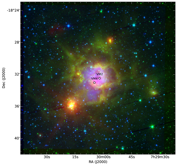
Figure 1: Color-composite image obtained by using the UK Schmidt telescope (UKST) H$\alpha$ (blue), $Spitzer$ 4.5 $\mu$m (green) and $WISE$ 22 $\mu$m (red) images of the $\sim 18^{\prime}.5\times 18^{\prime}.5$ FOV around Sh 2-305 H ii region. The locations of two massive stars VM2 (O9.5) and VM4 (O8.5) are also shown in the figure by black circles (Vogt & Moffat, 1975; Chini & Wink, 1984).

2 Observation and data reduction

2.1 Optical photometric data

The broad-band $UBV{(RI)}_{c}$ optical observations of the Sh 2-305 were taken using 2K$\times$2K CCD camera mounted on f/4 Cassegrain focus of the 1.3 m Devasthal fast optical telescope (DFOT) of Aryabhatta Research Institute of Observational Sciences (ARIES), Nainital, India. The color-composite image of the observed region of Sh 2-305 obtained by combining the UK Schmidt telescope (UKST) H$\alpha$ (blue color), $Spitzer$ 4.5 $\mu$m (green color), and $WISE$ 22 $\mu$m (red color) images is shown in Figure 1. With a pixel size of 13.5 $\mu$m $\times$ 13.5 $\mu$m and a plate scale of $0^{\prime\prime}$.54 pixel^-1, the CCD covers a field-of-view (FOV) of $\sim 18^{\prime}.5\times 18^{\prime}.5$ on the sky. The readout noise and gain of the CCD are 8.29 $e^{-}$ and 2.2 $e^{-}$/ADU, respectively. The average seeing during the observing nights was $\sim 2^{\prime\prime}$. The log of observations is given in Table 1. Along with the object frames, several bias and flat frames were also taken during the same night. The broad-band $UBV{(RI)}_{c}$ observations of the Sh 2-305 were standardized by observing stars in the SA 98 field ($\alpha_{J2000}$: 06^h52^m14^s, $\delta_{J2000}$: -00$\arcdeg$18$\arcmin$59$\arcsec$, Landolt, 1992) on the same night.

Initial processing of the data frames (i.e., bias subtraction, flat fielding, etc.) was done using the IRAF and ESO-MIDAS data reduction packages. The frames in the same filter were average combined to increase the signal-to-noise ratio of the faint stellar sources. Photometry of the combined frames was carried out by using DAOPHOT-II software (Stetson, 1987). The point spread function (PSF) was constructed for each frame using several uncontaminated stars. We used the DAOGROW program for construction of an aperture growth curve required for determining the difference between the aperture and PSF magnitudes.

Using the standard magnitudes of stars located in the SA 98 field, we have calibrated the stellar sources in the Sh 2-305. Calibration of the instrumental magnitudes to the standard system was done by using the procedures outlined by Stetson (1992). The calibration equations derived by the least-squares linear regression are as follows:

$$u=U+(4.776\pm 0.009)-(0.072\pm 0.007)(U-B)+(0.558\pm 0.011)X_{U},$$ (1)

$$b=B+(3.01\pm 0.006)-(0.147\pm 0.005)(B-V)+(0.319\pm 0.009)X_{B},$$ (2)

$$v=V+(2.467\pm 0.011)+(0.099\pm 0.007)(V-I_{c})+(0.216\pm 0.009)X_{V},$$ (3)

$$r_{c}=R_{c}+(2.067\pm 0.008)+(0.110\pm 0.012)(V-R_{c})+(0.148\pm 0.006)X_{R},$$ (4)

$$i_{c}=I_{c}+(2.592\pm 0.006)-(0.032\pm 0.004)(V-I_{c})+(0.114\pm 0.005)X_{I}$$ (5)

where $U,B,V,R_{c}$ and $I_{c}$ are the standard magnitudes and $u,b,v,r_{c}$ and $i_{c}$ are the instrumental aperture magnitudes normalized for the exposure time and $X^{\prime}s$ are the airmasses. The standard deviations of the standardization residual, $\Delta$, between standard and transformed $V$ magnitudes and $(U-B)$, $(B-V)$, $(V-I)$ and $(V-R)$ colors of standard stars are 0.006, 0.025, 0.015, 0.015 and 0.015 mag, respectively. In Figure 2 (left-hand panel), we show a comparison between the final standard magnitudes from our standardization process and the magnitudes from archive ‘APASS’. It can be seen that there is almost zero difference between the magnitudes. We have used only those stars for further analyses which are having photometric errors $<$0.1 mag. The photometry of the brightest stars that were saturated in long exposure frames, has been taken from short exposure frames. In total, 2646 stars were identified in the $\sim 18^{\prime}.5\times 18^{\prime}.5$ FOV of Sh 2-305 with detection limits of 21.92 mag and 19.78 mag in $V$ and $I_{c}$ bands, respectively.

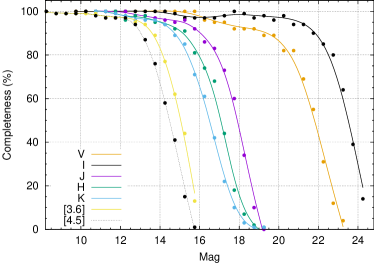
Figure 2: Left panel: Comparison between present photometry and that from ‘APASS’ in $V$ and $B$ bands. Right panel: Completeness levels as a function of magnitude derived from the artificial star experiments (ADDSTAR, see Section 2.4).

2.2 Near-infrared photometric data

NIR imaging data in $JHK$ bands were taken using TIFR Near Infrared Spectrometer and Imager (TIRSPEC) mounted on 2 m Himalayan $Chandra$ Telescope (HCT), Hanle, Ladakh, India. The detector array in the instrument is $1024\times 1024$ Hawaii-1 array covering 1 to 2.5 $\mu$m wavelength bands. With 0^′′.3 pixel^-1 resolution, the instrument provides a FOV of $307^{\prime\prime}\times 307^{\prime\prime}$ in the imaging mode (Ninan et al., 2014). As this FOV is not sufficient to cover the entire H ii region, we covered the entire region of our interest with five pointings in $J,H$ and $K$ filters. In each filter, 7 frames of 20 sec exposure were taken and each frame was created with 5 dithered images. The complete log of observation is given in Table 1. We followed the usual stpdf for NIR data: dark subtraction, flat-fielding, sky subtraction, alignment and averaging of sky-subtracted frames for each filter separately. The sky frames were generated by median combining the dithered frames and were subtracted from the science images. The final instrumental magnitudes (PSF magnitudes) were determined by the same procedure as done for optical data. Calibration of instrumental magnitudes to the standard system was done by using 2MASS point source catalog (PSC) through following transformation equations

$$(J-K)=(0.90\pm 0.05)\times(j-k)+(0.69\pm 0.02)$$ (6)

$$(H-K)=(0.98\pm 0.02)\times(h-k)+(0.68\pm 0.01)$$ (7)

$$(K-k)=(0.10\pm 0.06)\times(H-K)+(-4.88\pm 0.03)$$ (8)

where, $JHK$ and $jhk$ are the standard magnitudes of the stars taken from 2MASS catalog and instrumental magnitudes from HCT data, respectively. Because of the higher number of detected stars in $K$ and $H$ bands, we have used the $H-K$ color to calibrate the $K$ magnitude. Astrometry of the stars was done using the Graphical Astronomy and Image Analysis Tool with a rms noise of the order of $\sim$0^′′.3. We merged the sources detected in different bands with a matching radius of 1^′′. In our final NIR source catalog, we have included only those stars which are detected at least in $K$ and $H$ bands and have magnitude uncertainties less than $0.2$ mag. As the stars having $K$ band magnitudes less than 11 mag are saturated in our observations, we have taken magnitudes of those stars from the 2MASS catalog. Our final catalog contains $1812$ stars (upto $K$$\sim$18.1 mag) located in the inner region ($\sim 10^{\prime}\times 10^{\prime}$ FOV) of Sh 2-305 (cf. Figure 3).

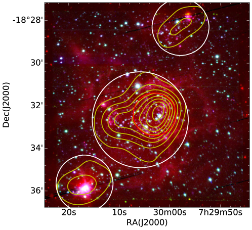
Figure 3: Color-composite image (blue: $J$-band, green: $K$-band, and red: WISE $4.6$ $\mu$m) of Sh 2-305 ($\sim 10^{\prime}\times 10^{\prime}$) covered in TIRSPEC NIR observations. The white circles represent three sub-clusterings identified in the present analysis. The red circle is the core region of the central clustering (cf. Section 3.1). The stellar surface density of the NIR sources generated using nearest neighbor method (cf. Section 3.1) is shown with the yellow contours.

2.3 Mid infrared photometric data

Sh 2-305 is observed by the $Spitzer$ space telescope on 2011 August 09 (program ID:61071; PI: Whitney Barbara A) with Infrared Array Camera (IRAC) at 3.6 $\micron$ and 4.5 $\micron$. We obtained the basic calibrated data (BCD) of the region from the Spitzer data archive. The exposure time of each BCD was 5 sec. To create final mosaicked images, we used 215 and 218 BCDs in 3.6 $\micron$ and 4.5 $\micron$, respectively. Mosaicking was performed using the MOPEX software provided by the Spitzer Science Center. All of our mosaics were built at the native instrument resolution of 1^′′.2 pixel^-1 with the standard BCDs. All the mosaics in different wavelengths are then aligned and trimmed to cover the region observed in optical wavelengths ($\sim 18^{\prime}.5\times 18^{\prime}.5$ around Sh 2-305; cf. Figure 1). These trimmed images have been used for further analyses.

In case of crowded and nebulous star-forming / H ii regions, we prefer $PSF$ photometry on IRAC data as explained in Sharma et al. (2012, 2016, 2017) and Panwar et al. (2014, 2017). Therefore, we used the DAOPHOT package available with the IRAF photometry routine to detect sources and to perform photometry in each IRAC band images. The full width at half maxima (FWHM) of each detection is measured and all detections with a FWHM $>$ 3^′′.6 are considered resolved and removed. The detected sources are also examined visually in each band to remove non-stellar objects and false detections. Aperture photometry for well isolated sources was done by using an aperture radius of 3^′′.6 with a concentric sky annulus of the inner and outer radii of 3^′′.6 and 8^′′.4, respectively. We adopted the zero-point magnitudes for the standard aperture radius (12^′′) and background annulus of (12^′′-22^′′.4) of 19.67 and 18.93 in the 3.6 $\micron$ and 4.5 $\micron$ bands, respectively. Aperture corrections were also made by using the values described in IRAC Data Handbook (Reach et al., 2006). In order to avoid source confusion due to crowding, the PSF photometry for all the sources was carried out. The necessary aperture corrections for the PSF photometry were then calculated from the selected isolated sources and were applied to the PSF magnitudes of all the sources. The sources with photometric uncertainties $<0.2$ mag in each band were considered for further analyses. Present photometry is found to be comparable to those available in the $Spitzer$ archive. A total of 2246 sources were detected upto $16.26$ mag and $15.67$ mag in the 3.6 $\micron$ and 4.5 $\micron$ bands, respectively. The NIR (2MASS and TIRSPEC) and optical counterparts of these IRAC sources were then searched within a matching radius of 1^′′.

2.4 Completeness of the photometric data

The photometric data may be incomplete due to various reasons, e.g., nebulosity, crowding of the stars, detection limit, etc. In particular, it is very important to know the completeness limits in terms of mass. The $IRAF$ routine $ADDSTAR$ was used to determine the completeness factor (CF) (for details, see Sharma et al., 2008). Briefly, in this method artificial stars of known magnitudes and positions are randomly added in the original frames and then these artificially generated frames are re-reduced by the same procedure as used in the original reduction. The ratio of the number of stars recovered to those added in each magnitude gives the CF as a function of magnitude. The CF as a function of magnitudes in different bands are given in Figure 2 (right-hand panel). In Table 2, we have listed the number of sources detected in different wavelengths along with detection and completeness limits of the multiwavelength photometric data collected in the present study.

2.5 Archival data

We have also used the 2MASS NIR (JHK_s) point source catalog (PSC) (Cutri et al., 2003) for the Sh 2-305. This catalog is reported to be 99$\%$ complete down to the limiting magnitudes of 15.8, 15.1 and 14.3 in the $J$, $H$ and $K_{s}$ band, respectively. We have selected only those sources which have NIR photometric accuracy $<$ 0.2 mag and detection in at least $H$ and $K_{s}$ bands.

The Wide-field Infrared Survey Explorer (WISE) is a 40 cm telescope in low-Earth orbit that surveyed the whole sky in four mid-infrared bands at 3.4, 4.6, 12, and 22 $\mu$m (namely $W1$, $W2$, $W3$, and $W4$ bands) with nominal angular resolutions of 6^′′.1, 6^′′.4, 6^′′.5, and 12^′′.0 in the respective bands (Wright et al., 2010). In this paper, we make use of the AllWISE catalog of the WISE survey data (Wright et al., 2010). AllWISE catalog is available via IRSA, the NASA/IPAC Infrared Science Archive. This catalog also includes the 2MASS $JHK_{s}$ magnitudes of the respective WISE sources.

3 Results and Analysis

3.1 Stellar clustering/groupings in the H ii region

A comparison between the stellar density distribution and the molecular cloud structure can provide the link between star formation, gas expulsion, and the dynamics of the clusters (Chen et al., 2004; Gutermuth et al., 2005; Sharma et al., 2006). To study the stellar surface density distribution in the Sh 2-305, we have generated surface density maps by performing nearest neighbor (NN) method on the 2MASS NIR catalog. We varied the radial distance in order to encompass the 20^th nearest star detected in 2MASS and computed the local surface density in a grid size of 6^′′. The density contours derived by this method are plotted in Figure 3 as yellow curves smoothened to a grid of size $3\times 3$ pixels. The lowest contour is 1$\sigma$ above the mean of stellar density (i.e. 7 stars/pc² at a distance of $3.7$ kpc, see Sec. 3.3) and the step size is equal to 1$\sigma$ (2.5 stars/pc² at $3.7$ kpc). The isodensity contours easily isolate the central sub-clustering (i.e., Mayer 3) of stars along with two highly elongated sub-structures in north-west and south-east directions of the central cluster.

The three sub-clusterings identified are encircled in Figure 3. The radius of the central sub-clustering i.e., ‘Mayer 3 cluster’ is 2^′.25, whereas for the other two sub-clusterings it is 1^′.3. The stellar density in the central cluster ‘Mayer 3’ region is significantly higher than for the other two sub-clusterings and its peak seems to be slightly off-center to the cluster. The stellar core region of ‘Mayer 3’ cluster is also shown by a red circle of $\sim 1^{\prime}$ radius in Figure 3. The central coordinates of the circular area for the north-west, center and south-east sub-clusterings are $\alpha_{2000}$: 07^h29^m57^s.9, $\delta_{J2000}$: -18$\arcdeg$28$\arcmin$18$\arcsec$; $\alpha_{2000}$: 07^h30^m05^s.9, $\delta_{J2000}$: -18$\arcdeg$32$\arcmin$39$\arcsec$; and $\alpha_{2000}$: 07^h30^m16^s.9, $\delta_{J2000}$: -18$\arcdeg$35$\arcmin$39$\arcsec$, respectively. We also define a bigger circular area of radius 5^′.65 centered at $\alpha_{2000}$: 07^h30^m05^s.9, $\delta_{J2000}$: -18$\arcdeg$32$\arcmin$15$\arcsec$ as a boundary of the Sh 2-305 H ii region (whole region), which encloses all of these sub-clusterings.

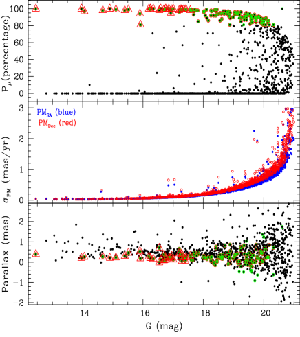
Figure 4: Left panel: PM vector-point diagrams (VPDs; top sub-panels) and Gaia DR2 $G$ vs. $(G_{BP}-G_{RP})$ CMDs (bottom sub-panels) for stars located in the Mayer 3 cluster region. The left sub-panels show all stars, while the middle and right sub-panels show the probable cluster members and field stars. Right panel: Membership probability P_μ, PM errors $\sigma_{PM}$ and parallax of stars as a function of $G$ magnitude for stars in the Mayer 3 cluster region. The probable member stars (P${}_{\mu}>$80 %) are shown by green circles while 35 members of the Sh 2-305 having parallax values with good accuracy taken from Bailer-Jones et al. (2018), are shown by red triangles.

3.2 Membership probability of stars in the Mayer 3 cluster

Gaia DR2 has opened up the possibility of an entirely new perspective on the problem of membership determination in cluster studies by providing the new and precise parallax measurements upto very faint limits. As there is a clear clustering of stars in the central region of Sh 2-305 (Mayer 3), $Gaia$ proper motion (PM) data located within this region (cf. Section 3.1, radius $<$ 2^′.25) and having PM error $\sigma_{PM}<$3 mas/yr are used to determine membership probability of stars located in this region. Proper motions (PMs), $\mu_{\alpha}$cos($\delta$) and $\mu_{\delta}$, are plotted as vector-point diagrams (VPDs) in the top sub-panels of Figure 4 (left panel). The bottom sub-panels show the corresponding $G_{(330-1050nm)}$ versus $G{{}_{BP(330-680nm)}}-G_{{RP(630-1050nm)}}$ Gaia color-magnitude diagrams (CMDs). The left sub-panels show all stars, while the middle and right sub-panels show the probable cluster members and field stars. A circular area of a radius of 0.6 mas yr^-1 around the cluster centroid in the VPD of PMs has been selected visually to define our membership criterion. The chosen radius is a compromise between loosing cluster members with poor PMs and including field stars sharing mean PM. The CMD of the most probable cluster members is shown in the lower-middle sub-panel. The lower-right sub-panel represents the CMD for field stars. Few cluster members are visible in this CMD because of their poorly determined PMs. The tight clump centering at $\mu_{xc}$ = -1.87 mas yr^-1, $\mu_{yc}$ = 2.31 mas yr^-1 and radius = 0.6 mas yr^-1 in the top-left sub-panel represents the cluster stars, and a broad distribution is seen for the probable field stars. Assuming a distance of $\sim$ 3.7 kpc (cf. Section 3.3) and a radial velocity dispersion of 1 kms^-1 for open clusters (Girard et al., 1989), the expected dispersion ($\sigma_{c}$) in PMs of the cluster would be $\sim$0.06 mas yr^-1. For remaining stars (probable field stars), we have calculated: $\mu_{xf}$ = -2.02 mas yr^-1, $\mu_{yf}$ = 3.31 mas yr^-1, $\sigma_{xf}$ = 1.77 mas yr^-1 and $\sigma_{yf}$ = 3.57 mas yr^-1. These values are further used to construct the frequency distributions of cluster stars ($\phi_{c}^{\nu}$) and field stars ($\phi_{f}^{\nu}$) by using the equations given in Yadav et al. (2013) and then the value of membership probability (ratio of distribution of cluster stars with all the stars) of all the stars within Sh 2-305 (Section 3.1, radius$<$ 5^′.65), is given by using the following equation:

$$P_{\mu}(i)={{n_{c}\times\phi^{\nu}_{c}(i)}\over{n_{c}\times\phi^{\nu}_{c}(i)+n_{f}\times\phi^{\nu}_{f}(i)}}$$ (9)

where $n_{c}$ (=0.26) and $n_{f}$(=0.74) are the normalized number of stars for the cluster and field ($n_{c}$+$n_{f}$ = 1), respectively. The membership probability estimated as above, errors in the PM, and parallax values are plotted as a function of $G$ magnitude in Figure 4 (right-hand panel). As can be seen in this plot, a high membership probability (P${}_{\mu}>$ 80 %) extends down to $G\sim$20 mag. At brighter magnitudes, there is a clear separation between cluster members and field stars supporting the effectiveness of this technique. Errors in PM become very high at faint limits and the maximum probability gradually decreases at those levels. Except few outliers, most of the stars with high membership probability (P${}_{\mu}>$ 80 %) are following a tight distribution. Finally, from the above analysis, we were able to calculate membership probability of 1000 stars in the Sh 2-305. Out of these, 137 stars were considered as members of the Sh 2-305 based on their high probability P_μ ($>$80 %) and the parallax values (black dots with green circles around them, shown in Figure 4 right-hand panel). The details of these member stars are given in Table 3. 131 of these member stars have optical counterparts from the present photometry, identified within a search radius of one arcsec.

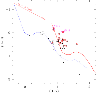
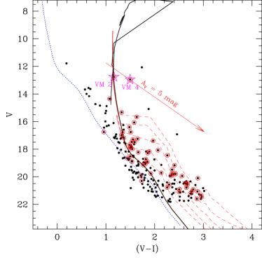
Figure 5: Left panel: $(U-B)$ vs. $(B-V)$ TCD for the sources in the Mayer 3 cluster region (radius $<$ 2^′.25, black dots). The identified member stars using PM analysis are also plotted by red circles. The dotted blue curve represents the intrinsic ZAMS for $Z=0.02$ by Schmidt-Kaler (1982). The red continuous curve represents the ZAMS shifted along the reddening vector (see text for details) by $E(B-V)_{cluster}$ = 1.17 mag for the stars associated with the cluster. Right panel: $V$ vs. $(V-I)$ CMD for the same sources. The MS isochrone for 1 Myr (red curve) and 5 Myr (black curve) by Marigo et al. (2008) and PMS isochrones of 0.5, 1, 2, 5, 10 Myr by Siess et al. (2000, dashed red curves), corrected for the distance of 3.7 kpc and reddening $E(B-V)_{cluster}=1.17$ mag, are also shown. The blue dotted curve is the 1 Myr MS isochrone by Marigo et al. (2008) corrected for the distance of 1.2 kpc and zero reddening. We have also plotted the location of two massive stars by star symbols in the figures.

3.3 Reddening, distance and age of the Mayer 3 cluster

The reddening and distance of a cluster can be derived quite accurately by using the two-color diagrams (TCDs) and CMDs of their member stars (cf., Phelps & Janes, 1994; Sharma et al., 2006). Left-hand panel of Fig. 5 shows the $(U-B)$ versus $(B-V)$ TCD with the intrinsic zero-age-main-sequence (ZAMS) shown in blue dotted curve, taken from Schmidt-Kaler (1982), along with stars located within the boundary of the central cluster Mayer 3 (i.e., radius$<$ 2^′.25) denoted by black dots. We have also over-plotted the member stars identified by using PM data as red circles. The distribution of the stars shows a large spread along the reddening vector, indicating heavy differential reddening in this region. It reveals two different populations, one (mostly black dots) distributed along the ZAMS and another (consisting mostly red circles) showing a large spread in their reddening value. The former having negligible reddening must be the foreground population and the latter could be member stars. If we look at the MIR image of this region (Figure 1), we see several dust lanes along with enhancements of nebular emission at several places. Both of them are likely responsible for the large spread in the reddening of member stars population. The ZAMS from Schmidt-Kaler (1982) is shifted along the reddening vector with a slope of $E(U-B)/E(B-V)$ = 0.72 (corresponding to $R_{V}$ $\sim$ 3.1, cf. Appendix A) to match the distribution of stars showing the minimum reddening among the member stars population (dotted curve). The other member population may be embedded in the nebulosity of this H ii region. The foreground reddening value, $E(B-V)_{cluster}$, thus comes to be $\sim$ 1.17 mag and the ZAMS reddened by this amount is shown by a red continuous curve. The approximate error in the reddening measurement ‘$E(B-V)$’ is $\sim$ 0.1 mag, as has been determined by the procedure outlined in Phelps & Janes (1994).

In the literature, the distance estimation of Mayer 3 cluster varies from 2.5 to 5.2 kpc (cf. Vogt & Moffat, 1975; Chini & Wink, 1984; Russeil et al., 1995; Bica et al., 2003; Azimlu & Fich, 2011; Kharchenko et al., 2016) which are derived both photometrically and spectroscopically. To confirm the distance to this cluster, we have used the $V$ versus $(V-I)$ CMD, generated from our deep optical photometry of the stars located in the cluster region (radius $<$ 2^′.25, black dots), as shown in Figure 5 (right-hand panel). The distribution of member stars identified using PM data analysis (red circles) have also been shown in the CMD. Here also, the CMD reveals two different populations, one (mostly black dots) for foreground stars having almost zero reddening value (near dotted curve) and another (mostly red circles) for the cluster members at higher reddening value and a larger distance.

The CMD for cluster members displays a few main-sequence (MS) stars upto $V\sim$18 mag and pre-main sequence (PMS) stars at fainter end. The dotted curve represents a ZAMS isochrone derived from Marigo et al. (2008, age=1 Myr), randomly corrected for a distance of 1.2 kpc, which is matching well with the foreground stars. We can further visually fit this MS isochrone to the distribution of member stars quite nicely, which is corrected for extinction ($E(B-V)_{cluster}$=1.17 mag) and distance ($\sim$ 3.7 kpc; solid red curve). The dashed red curves are the PMS isochrones of 0.5, 1, 2, 5 and 10 Myrs by Siess et al. (2000), corrected for the same distance (3.7 kpc) and extinction value ($E(B-V)_{cluster}$ = 1.17 mag).

An upper limit to the age of the cluster can be established from the most massive member star. The location of most massive star VM4 (O8.5) in the $V$ versus $(V-I)$ CMD is traced back along the reddening vector to the turn-off point in the MS, which is equivalent to a 5 Myr old isochrone (cf. black curve in Figure 5 right panel). Assuming a coeval star-formation event, the oldest stellar content in the Mayer 3 cluster must therefore be younger than 5 Myr.

To confirm further and establish the relation between the central cluster ‘Mayer 3’ and the Sh 2-305 H ii region, we have calculated the mean of the distances of 35 members of the Sh 2-305 having parallax values with good accuracy (i.e., error$<$ 0.1 mas) as 3.7$\pm$1.1 kpc (Bailer-Jones et al., 2018). Clearly, this value is in agreement with distance of the central cluster Mayer 3 derived earlier, indicating that both cluster and the H ii region Sh 2-305 are associated to each other at similar distance of 3.7 kpc.

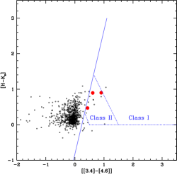
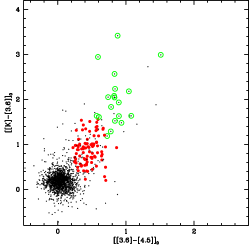
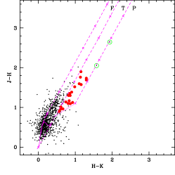
Figure 6: Left panel: ${[[3.4]-[4.5]]}$ vs. ${[H-K_{s}]}$ TCD of all the sources identified within the selected $\sim 18^{\prime}.5\times 18^{\prime}.5$ FOV of the Sh 2-305 region. The YSOs are classified as Class I and Class II based on the color criteria by Koenig & Leisawitz (2014). Middle panel: ${[[K]-[3.6]]}_{0}$ vs. ${[[3.6]-[4.5]]}_{0}$ TCD for the sources in the same FOV. The YSOs classified as Class I and Class II, are based on the color criteria by Gutermuth et al. (2009). Right panel: ${[H-K]}$ vs. ${[J-H]}$ TCD for the sources in the same FOV (Ojha et al., 2004a). The continuous and thick red dashed curves represent the reddened MS and giant branches (Bessell & Brett, 1988), respectively. The dotted red line indicates the locus of dereddened CTTSs (Meyer et al., 1997). The parallel red dashed lines are the reddening lines drawn from the tip (spectral type M4) of the giant branch (left reddening line), from the base (spectral type A0) of the MS branch (middle reddening line) and from the tip of the intrinsic CTTS line (right reddening line). The crosses on the reddening lines show an increment of $A_{V}$ = 5 mag. The YSOs classified as Class i and Class ii are shown with red dots and green circles, respectively.

3.4 Identification of YSOs in the Sh 2-305 region

Identification and characterization of YSOs in star-forming regions (SFRs) hosting massive stars are essential stpdf to examine the physical processes that govern the formation of the next generation stars in such regions. In this study, we have used NIR and MIR observations of the Sh 2-305 ($\sim$ $18^{\prime}.5\times 18^{\prime}.5$ FOV) to identify candidate YSOs based on their excess IR emission. The identification and classification schemes are described as below.

• Using AllWISE catalog of WISE MIR data: The location of WISE bands in the MIR matches where the excess emission from cooler circumstellar disk/envelope material in young stars begins to become significant in comparison to the stellar photosphere. The procedures outlined in Koenig & Leisawitz (2014) have been used to identify YSOs in this region. We refer figure 3 of Koenig & Leisawitz (2014) to summarize the entire scheme. This method includes photometric quality criteria for different WISE bands as well as the selection of candidate extragalactic contaminants (AGN, AGB stars and star-forming galaxies). Figure 6 (left panel) shows the $[[3.4]-[4.6]]$ versus $(H-K_{s})$ TCD for all the sources in the region, where 3 probable YSOs shown by red dots are classified as Class ii source.

• Using $Spitzer$ MIR data: As we have photometric data for two IRAC bands 3.6 $\mu$m and 4.5 $\mu$m, this along with $K$ band is used to plot the de-reddened [[3.6] - [4.5]]₀ versus [K - [3.6]]₀ TCD as shown in Figure 6 (middle panel). The procedure outlined in Gutermuth et al. (2009) has been used to de-redden and classify sources as Class i (green circles, 20) and Class ii (red dots, 95) YSOs. This method also includes photometric quality criteria for different IRAC bands as well as the selection of candidate contaminants (PAH galaxies and AGNs).

• Using TIRSPEC and 2MASS NIR data: We combined TIRSPEC NIR photometry (cf. Section 2.2) with the 2MASS catalog to make a final catalog covering the $18^{\prime}.5\times 18^{\prime}.5$ FOV of the selected Sh 2-305 region. Then those stars whose corresponding counterparts were found in $Spitzer$ or WISE catalog were removed from this catalog to further identify YSOs which are not detected in the WISE or $Spitzer$ photometry, by using NIR TCD (Ojha et al., 2004a). In Figure 6 (right panel) we have plotted NIR TCD of the above stars. The solid and thick broken curves represent the unreddened MS and giant branches (Bessell & Brett, 1988). The dotted line indicates the locus of unreddened Classical T Tauri Stars (CTTS) (Meyer et al., 1997). The parallel dashed lines are the reddening vectors drawn from the tip of the giant branch (upper reddening line), from the base of the MS branch (middle reddening line) and from the tip of the intrinsic CTTS line (lower reddening line). We classified the sources according to their locations in the diagram (Ojha et al., 2004a; Sharma et al., 2007; Pandey et al., 2008). The sources occupying the location between the upper and middle reddening lines (‘F’ region) are considered to be either field stars or Class iii sources and/or Class ii sources with small NIR excess. The sources located between the middle and lower reddening lines (‘T’ region) are considered to be mostly CTTS (or Class ii sources) with large NIR excess. However, we note that there may be overlap of the Herbig Ae/Be stars in the ‘T’ region (Hillenbrand, 2002). Sources that are located in the region redward of the lower reddening vector (‘P’ region) most likely are Class i objects. In Figure 6, we have shown the location of identified Class i sources with green circles (2) and Class ii objects with red dots (21).

Finally, we have merged all the YSOs identified based on their IR excess emission by using different schemes to have a final catalog of 116 YSOs in the $\sim 18^{\prime}.5\times 18^{\prime}.5$ FOV around Sh 2-305. The positions, magnitudes in different NIR/MIR bands of these YSOs, along with their classification are given in Table 4. Optical counterparts for $28$ of these YSOs were also identified by using a search radius of 1^′′ and their optical magnitudes and colors are given in Table 5.

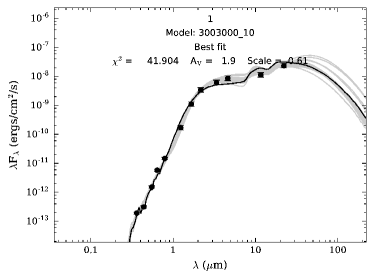
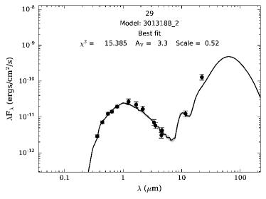
Figure 7: Sample SEDs for Class i (left-hand panel) and Class ii (right-hand panel) sources created by the SED fitting tools of Robitaille et al. (2007). The black curve shows the best fit and the gray curves show the subsequent well fits. The filled circles with error bars denote the input flux values.

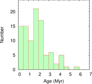
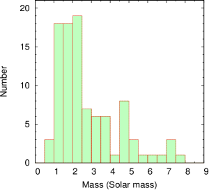
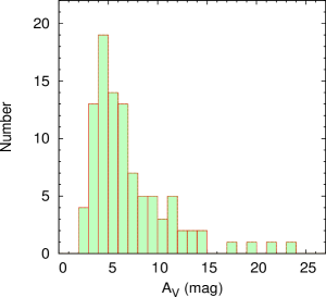
Figure 8: Histograms showing the distribution of the ages (left-hand panel), masses (middle panel) and extinction values ‘$A_{V}$’ (right-hand panel) of the YSOs (98) in the Sh 2-305 as derived from the SED fitting analysis (cf. Section 3.5).

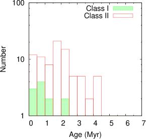
Figure 9: Left panel: Cumulative distribution of Class i (solid line) and Class ii (dotted line) YSOs as a function of their age. Right panel: Age distribution of Class i (filled histogram) and Class ii (un-filled histogram) YSOs.

3.5 Physical properties of YSOs

Since the aim of this work is to study the star formation activities in the Sh 2-305, the information regarding individual properties of the YSOs is vital, which can be derived by using the SED fitting analysis. We constructed SEDs of the YSOs using the grid models and fitting tools of Whitney et al. (2003a, b, 2004) and Robitaille et al. (2006, 2007) for characterizing and understanding their nature. This method has been extensively used in our previous studies (see. e.g., Jose et al., 2016; Sharma et al., 2017, and references therein). We constructed the SEDs of the YSOs using the multiwavelength data (optical to MIR wavelengths, i.e. 0.37, 0.44, 0.55, 0.65, 0.80, 1.2, 1.6, 2.2, 3.4, 3.6, 4.5, 4.6, 12 and 22 $\mu m$) and with a condition that a minimum of 5 data points should be available. Out of 116 YSOs, 98 satisfy this criterion and therefore are used in the further analysis. The SED fitting tool fits each of the models to the data allowing the distance and extinction as free parameters. The input distance range of the Sh 2-305 is taken as 3.3 - 4.1 kpc keeping in mind the error associated with distance, Since, this region is highly nebulous, we varied $A_{V}$ in a broader range i.e. from 3.6 (foreground reddening) to 30 mag (see also, Samal et al., 2012; Jose et al., 2013; Panwar et al., 2014). We further set photometric uncertainties of 10% for optical and 20% for both NIR and MIR data. These values are adopted instead of the formal errors in the catalog in order to minimize any possible bias in the fitting that is caused by underestimating the flux uncertainties. We obtained the physical parameters of the YSOs using the relative probability distribution for the stages of all the ‘well-fit’ models. The well-fit models for each source are defined by $\chi^{2}-\chi^{2}_{min}\leq 2N_{data}$, where $\chi^{2}_{min}$ is the goodness-of-fit parameter for the best-fit model and $N_{data}$ is the number of input data points.

In Figure 7, we show example SEDs of Class i (left panel) and Class ii (right panel) sources, where the solid black curves represent the best-fit and the gray curves are the subsequent well-fits. As can be seen, the SED of the Class I source shows substantial MIR excess in comparison to the Class ii source due to its optically thick disk. From the well-fit models for each source derived from the SED fitting tool, we calculated the $\chi^{2}$ weighted model parameters such as the $A_{V}$, stellar mass and stellar age of each YSO and they are given in Table 6. The error in each parameter is calculated from the standard deviation of all well-fit parameters. Histograms of the age, mass and $A_{V}$ of these YSOs are shown in Figure 8. It is found that $\sim$91% (89/98) of the sources have ages between 0.1 to 3.5 Myr. The masses of the YSOs are between 0.8 to 16.2 M_⊙, a majority ($\sim$80%) of them being between 0.8 to 4.0 M_⊙. These age and mass ranges are comparable to the typical age and mass of TTSs. The $A_{V}$ distribution shows a long tail indicating its large spread from $A_{V}$=2.2 - 23 mag, which is consistent with the nebulous nature of this region. The average age, mass and extinction ($A_{V}$) for this sample of YSOs are 1.8 Myr, 2.9 M_⊙ and 7.1 mag, respectively.

The evolutionary class of the selected 116 YSOs, given in the Table 4, reveals that $\sim$ 17% and $\sim$ 83 % sources are Class i and Class ii YSOs, respectively. In Figure 9 (left panel), we have shown the cumulative distribution of Class i and Class ii YSOs as a function of their ages, which manifests that Class i sources are relatively younger than Class ii sources as expected. We have performed a Kolmogorov-Smirnov (KS) test for this age distribution. The test indicates that the chance of the two populations having been drawn from the same distribution is $\sim$4%. The right-hand panel of Figure 9 plots the distribution of ages for the Class i and Class ii sources. The distribution of the Class i sources shows a peak at a very young age, i.e., $\sim$0.50-0.75 Myr, whereas that of the Class ii sources peaks at $\sim$1.50-1.75 Myr. Both of these figures show an approximate age difference of $\sim$1 Myr between the Class i and Class ii sources. Here it is worthwhile to take note that Evans et al. (2009) through c2d $Spitzer$ Legacy projects studied YSOs associated with five nearby molecular clouds and concluded that the life time of the Class i phase is 0.54 Myr. The peak in the histogram of Class i sources agrees well with them (see also Sharma et al., 2017).

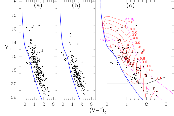
Figure 10: Left panel : $V_{0}$ vs. $(V-I_{c})_{0}$ CMD for (a) stars in the Mayer 3 cluster region, and (b) stars in the reference region. (c) is a statistically cleaned $V_{0}$ vs. $(V-I_{c})_{0}$ CMD for stars lying in the Mayer 3 cluster region. Red circles (ages $\leq$ 3.5 Myr) are used to estimate the MF of the region. The isochrone of 2 Myr by Marigo et al. (blue curve, 2008) and the PMS isochrones of 0.1 and 3.5 Myrs along with the evolutionary tracks for different masses by Siess et al. (magenta dashed and red curves, 2000) are also shown. All the curves are corrected for the distance of 3.7 kpc. The back horizontal line represents the completeness limit of the data (upto 90%) after taking into account the average extinction of the YSOs. Right panel: A plot of the MF for the statistically cleaned CMD for the stellar sources in the Mayer 3 cluster region. Log $\phi$ represents log($N$/dlog $m$). The error bars represent $\pm\sqrt{N}$ errors. The solid line shows the least squares fit to the MF distribution (black dots). Open squares are the data points falling below the completeness limit of 0.8 M_⊙. Open circles are the data points near turn-off point in the MF distribution and are not used in the fitting.

Figure 11: (a) Comparison of the observed KLF in the reference field and the simulated KLF from star count modeling. The filled circles denote the observed K-band star counts in the reference field, and triangles represent the simulation from the Galactic model (see the text). The star counts are number of stars per square degree and the error bars represent $\sqrt{N}$ errors. The KLF ($\alpha$, see Section 4.4) of the reference field (solid line) is $0.36\pm 0.07$. The simulated model is also giving the same value of slope $(0.34\pm 0.01)$. (b) The corrected KLF for the probable members in the central cluster ‘Mayer 3’ (slope: $0.40\pm 0.04$). The straight line is the least-square fit to the data points in the range 12.5-15.5 mag.

3.6 Mass Function (MF) and K-band Luminosity Function (KLF)

The MF is an important statistical tool to understand the formation of stars (Sharma et al., 2017, and references therein). The MF is often expressed by a power law, $N(\log m)\propto m^{\Gamma}$ and the slope of the MF is given as: $\Gamma=d\log N(\log m)/d\log m$, where $N(\log m)$ is the number of stars per unit logarithmic mass interval. We have used our deep optical data to generate the MF of the Sh 2-305 region. For this, we have utilized the optical $V_{0}$ versus $(V-I_{c})_{0}$ CMDs of the sources in the target region and that of the nearby field region of equal area and decontaminated the former sources from foreground/background stars and corrected for data in-completeness using a statistical subtraction method already described in detail in our previous papers (cf. Sharma et al., 2007, 2012, 2017; Pandey et al., 2008, 2013; Chauhan et al., 2011; Jose et al., 2013). As an example, in Figure 10 (left panel), we have shown the $V_{0}$ versus $(V-I_{c})_{0}$ CMDs for the stars lying within the central cluster ‘Mayer 3’ in panel ‘a’ and for those in the reference field region selected as an annular region outside the boundary of Sh 2-305 region (cf. Section 3.1) in panel ‘b’. The magnitudes were corrected for the $A_{V}$ values derived from the reddening map (cf. Section 3.7). In panel ‘c’, we have plotted the statistically cleaned $V_{0}$ versus $(V-I_{c})_{0}$ CMD for the central cluster ‘Mayer 3’ which is showing the presence of PMS stars in the region. The ages and masses of the stars in this statistically cleaned CMD have been derived by applying the procedure described earlier in our previous papers (Chauhan et al., 2009; Sharma et al., 2017). For reference, the post-main-sequence isochrone for 2 Myr calculated by Marigo et al. (2008) (thick blue curve) along with the PMS isochrones of 0.1 and 3.5 Myr (purple curves) and evolutionary tracks of different masses (red curves) by Siess et al. (2000) are also shown in panel ‘c’. These isochrones are corrected for the distance of the Sh 2-305 (3.7 kpc, cf. Section 3.3). The corresponding MF has subsequently been plotted in Figure 10 (right panel) for the central cluster ‘Mayer 3’. For this, we have used only those sources which have ages equivalent to the average age of the optically identified YSOs combined with error (i.e., $\leq$3.5 Myr, cf. Table 6). Our photometry is more than 90% complete up to $V=21.5$ mag, which corresponds to the detection limit of 0.8 M_⊙ (cf. Figure 10 (left panel) ‘c’) PMS star of $\simeq$1.8 Myr age embedded in the nebulosity of $A_{V}\simeq$3.0 mag (i.e., the average values for the optically detected YSOs, cf. Table 6). We have applied a similar approach to derive MF of the southern clustering and the whole region of the Sh 2-305 (cf. Section 3.1) and their corresponding values of MF slopes in the mass range $1.5<M_{\odot}<6.6$ are given in Table 7. The MF of the northern clustering cannot be determined due to insignificant number of optically detected stars.

The KLF is also a powerful tool to investigate the IMF of young embedded clusters, and is related to IMF by a relation, $\alpha=\dfrac{-\Gamma}{2.5\beta}$, where $\alpha$, $\Gamma$ and $\beta$ are the slopes of KLF, IMF and mass-luminosity relationship, respectively (e.g., Lada et al., 1993; Lada & Lada, 2003; Ojha et al., 2004b; Sanchawala et al., 2007; Mallick et al., 2014). To take into account the foreground/background field star contamination, we used the Besançon Galactic model of stellar population synthesis (Robin et al., 2003) and predicted the star counts in both the cluster region and in the direction of the reference field. We checked the validity of the simulated model by comparing the model KLF with that of the reference field and found that the two KLFs match rather well (Figure 11a). An advantage of using the model is that, we can separate the foreground ($d<3.7$ kpc) and the background ($d>3.7$ kpc) field stars. The foreground extinction towards the cluster region is found to be $A_{V}\sim 3.63$ mag. The model simulations with $d<3.7$ kpc and $A_{V}$ = 3.63 mag give the foreground contamination, and that with $d>3.7$ kpc and $A_{V}$ = 3.63 mag the background population. We thus determined the fraction of the contaminating stars (foreground+background) over the total model counts. This fraction was used to scale the nearby reference region and subsequently the modified star counts of the reference region were subtracted from the KLF of the cluster to obtain the final corrected KLF. This KLF is expressed by the following power-law: ${{\rm{d}N(K)}\over{\rm{d}K}}\propto 10^{\alpha K}$, where ${\rm{d}N(K)}\over{\rm{d}K}$ is the number of stars per 0.5 magnitude bin and $\alpha$ is the slope of the power law. Figure 11b shows the KLF for the Mayer 3 cluster region. Similarly, we have derived KLF for other clusterings as well as the whole region (cf. Section 3.1) and their corresponding slope values in $K$-band completeness range of $12.5<K(mag)<15.5$ are given in Table 7.

3.7 Spatial distribution of molecular gas and YSOs in the region

In the Figure 12a, we present Herschel column density ($N(\mathrm{H}_{2})$) map of the Sh 2-305 region to examine the embedded structures. The spatial resolution of the map is $\sim$12^′′. Adopting the Bayesian PPMAP procedure operated on the Herschel data (Molinari et al., 2010a) at wavelengths of 70, 160, 250, 350 and 500 $\mu$m (Marsh et al., 2015, 2017), the Herschel temperature and column density maps were produced for the EU-funded ViaLactea project (Molinari et al., 2010b). The map is also overlaid with the NVSS radio continuum contours and the column density contour (at 6.5 $\times$ 10²¹ cm^-2) to enable us to study the distribution of embedded condensations/clumps against the ionized gas. In general, the $N(\mathrm{H}_{2})$ maps shows fragmented structures with several embedded dust clumps in the target region. The peak of the NVSS radio emission appears to be surrounded by the dust clumps. We have used clumpfind algorithm (Williams et al., 1994) to identify 25 clumps in the column density map of our selected target area. The boundary and the position of each clump are also shown in Figure 12b. The mass of each clump is determined and is listed in Table 8. In this connection, we employed the equation, $M_{area}=\mu_{H_{2}}m_{H}Area_{pix}\Sigma N(H_{2})$, where $\mu_{H_{2}}$ is the mean molecular weight per hydrogen molecule (i.e., 2.8), $Area_{pix}$ is the area subtended by one pixel (i.e., 6^′′/pixel), and $\Sigma N(\mathrm{H}_{2})$ is the total column density (see also Dewangan et al., 2017). Table 8 also contains an effective radius of each clump, which is provided by the clumpfind algorithm. The clump masses vary between 35 M_⊙ and 1565 M_⊙, and the most massive clump (ID = 2 in Table 8) lies in the northern direction of the region.

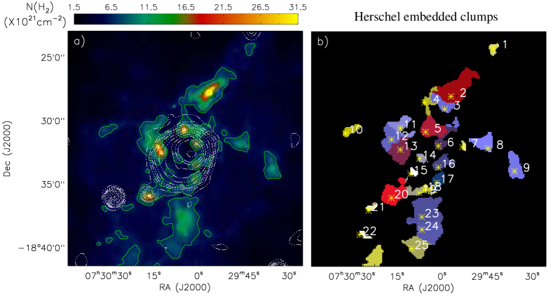
Figure 12: Left panel: $Herschel$ column density ($N(\mathrm{H}_{2})$) map of $\sim 18^{\prime}.5\times 18^{\prime}.5$ FOV of the Sh 2-305 region (see text for details). The map is also superimposed with the NVSS radio continuum contours (in white) and the column density contour (at 6.5 $\times$ 10²¹ cm^-2; in green). The NVSS 1.4 GHz contours are shown with levels of (0.45 mJy/beam) $\times$ (3, 10, 15, 20, 30, 50, 80, 120, 160, 200, 300). Right panel: The boundary of each identified clump and its position are highlighted along with its corresponding clump ID (see Table 8).

Figure 13 (top left panel) shows the color composite image generated using the WISE 12 $\mu$m (red), $Spitzer$ 4.5 $\mu$m (green) and $Spitzer$ 3.6 $\mu$m (blue) images of the Sh 2-305 region. We have also over-plotted the identified YSOs on the figure. The WISE 12 $\mu$m image covers the prominent PAH features at 11.3 $\mu$m, indicative of star formation (see e.g. Peeters et al., 2004). We can observe several filamentary structures in the 12 $\mu$m emission. The distribution of a majority of the YSOs belongs generally to these structures. The distributions of the gas and dust, seen by the MIR emissions in the 4.5 $\mu$m and 3.6 $\mu$m images, are well correlated with the distribution of YSOs. Figure 13 (top-left panel) reveals that the Sh 2-305 is a site of active star formation and there are three major groupings of YSOs, distributed from northern to southern directions in the region.

To study the density distribution of YSOs in the region, we have generated the surface density map (cf. Figure 13, red contours in the top right panel) using the nearest neighbor (NN) method (see Section 3.1), with a grid size of 6^′′ and 5^th nearest YSOs in an area $\sim 18^{\prime}.5\times 18^{\prime}.5$ of Sh 2-305. The lowest contour is 1$\sigma$ above the mean of YSO density (i.e. 1.8 stars/pc²) and the step size is equal to the 1$\sigma$ (1.3 stars/pc²).

We have also derived $A_{K}$ extinction map using the $(H-K)$ colors of the MS stars to quantify the amount of extinction and to characterize the structures of the molecular clouds (see also, Gutermuth et al., 2009, 2011; Jose et al., 2013; Sharma et al., 2016; Pandey et al., 2019). The sources showing excess emission in IR can lead to overestimation of extinction values in the derived maps. Therefore, to improve the quality of the extinction maps, the candidate YSOs and probable contaminating sources (cf. Section 3.4) must be excluded for the calculation of extinction. In order to determine the mean value of A_K, we used the NN method as described in detail in Gutermuth et al. (2005) and Gutermuth et al. (2009). Briefly, at each position in a uniform grid of 6^′′, we calculated the mean value of $(H-K)$ colors of five nearest stars. The sources deviating above 3$\sigma$ were excluded to calculate the final mean color of each point. To facilitate comparisons between the stellar density and the gas column density, we adopted the grids identical to the grid size of the stellar density map for this region. To convert $(H-K)$ color excesses into $A_{K}$, we used the relation $A_{K}$ = 1.82 $\times$ E$(H-K)$, where E$(H-K)$=$(H-K)$_obs - $(H-K)_{int}$, adopting the reddening law by Flaherty et al. (2007).

We have assumed $(H-K)_{int}$ = 0.2 mag as an average intrinsic color for all stars in young clusters (see. Allen et al., 2008; Gutermuth et al., 2009). To eliminate the foreground contribution in the extinction measurement, we used only those stars with $A_{K}>$ 0.15$\times$D, where D is the distance of the H ii region in kpc (Indebetouw et al., 2005); to generate the extinction map. The extinction map is plotted in Figure 13 (top right panel) as black contours. The lowest contour is 1$\sigma$ above the mean extinction value (i.e. $A_{V}$=6.8 mag) and the step size is equal to 1$\sigma$ (1.5 mag). The extinction map displays more or less a similar morphology around the region as in the $Herschel$ column density map.

Here, it is also worthwhile to note that the derived isodensity/$A_{K}$ values are the lower limits of their values as the sources with higher extinction may not be detected in our study. The isodensity contours of the YSOs are clearly showing three stellar groupings (similar to the surface density distribution of NIR sources shown in Figure 3), one in the central region comprising the Mayer 3 cluster, other in the north direction, and another in the south direction. The extinction map also has a north to south elongated morphology similar to the isodensity contours, however, the peak in the stellar density is slightly off from the peak in extinction contours.

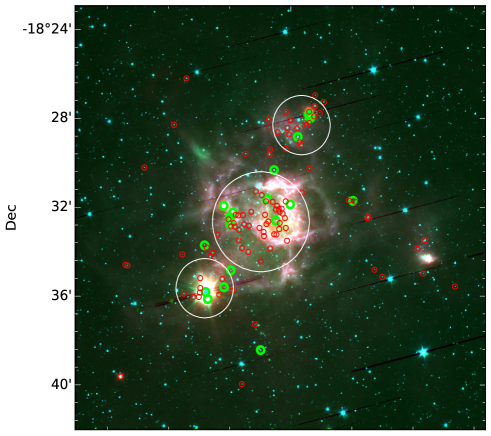
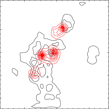
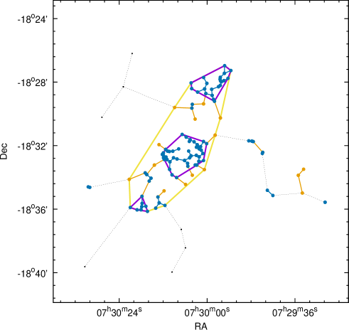
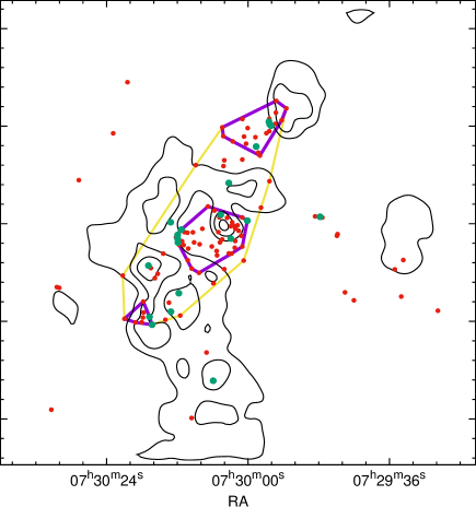
Figure 13: Top-left panel: Spatial distribution of YSOs superimposed on the $\sim 18^{\prime}.5\times 18^{\prime}.5$ color composite (red: WISE 12 $\mu$m, green: $Spitzer$ 4.5 $\mu$m, blue: $Spitzer$ 3.6 $\mu$m) image of the Sh 2-305 region. The locations of Class i (green circles) and Class ii (red circles) are also shown. The white circles represent the three clusters/clumps identified in the present analysis. Top-right panel: Isodensity contours for the YSOs distribution (red contours) and the reddening map (black contours) for the same region. Bottom-left panel: Minimal spanning tree (MST) for the identified YSOs in the same region along with the convex hull. The blue dots connected with solid blue lines and yellow dots connected with yellow lines are the branches smaller than the critical length for the cores and the active region, respectively. The identified cores and the active region are encircled with purple and yellow solid lines (i.e. Qhull), respectively. Bottom-right panel: Spatial correlation between the molecular material inferred from the extinction map (black contours) and the distribution of YSOs along with the identified cores and active region (thick purple and yellow lines, respectively).

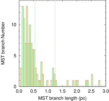
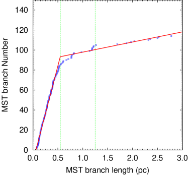
Figure 14: Histogram of MST branch length (left panel) and cumulative distribution functions (CDFs, right panel), used for the critical length analysis of YSOs. CDF plots have sorted length values on the vertical axis and a rising integer counting index on the horizontal axis. The red solid line is a two-line fit to the CDFs distribution. The inner and outer vertical green lines are the critical lengths obtained for the core and the active region (AR), respectively.

3.8 Extraction of YSO’s cores embedded in the molecular cloud

As discussed in previous sub-section, the Sh 2-305 contains three major sub-groups/cores of YSOs (cf. Figure 13, top left panel), presumably due to fragmentation of the molecular cloud. Physical parameters of these cores which might have formed in a single star-forming event, play a very important role in the study of star formation. Here, we have applied an empirical method based on the minimal sampling tree (MST) technique to isolate groupings (cores) of the YSOs from their diffuse distribution in this nebulous region (Gutermuth et al., 2009). This method effectively isolates the sub-structures without any type of smoothening and bias regarding the shapes of the distribution and it preserves the underlying geometry of the distribution (e.g., Cartwright & Whitworth, 2004; Schmeja & Klessen, 2006; Bastian et al., 2007, 2009; Gutermuth et al., 2009; Chavarría et al., 2014; Sharma et al., 2016; Pandey et al., 2019). In Figure 13 (bottom left panel), we have plotted the derived MSTs for the location of YSOs. The different color dots and lines are the positions of the YSOs and the MST branches, respectively. A close inspection of this figure reveals that the region exhibits different concentrations of YSOs distributed throughout the regions. In order to isolate these sub-structures, we have adopted a surface density threshold expressed by a critical branch length. In Figure 14 (left panel), we have plotted histograms between MST branch lengths and MST branch numbers for the YSOs. From this plot, it is clear that they have a peak at small spacings and a relatively long tail towards large spacings. These peaked distance distributions typically suggest a significant sub-region (or sub-regions) above a relatively uniform, elevated surface density. By adopting a MST length threshold, we can isolate those sources which are closer than this threshold, yielding populations of sources that make up local surface density enhancements. To obtain a proper threshold distance, we have fitted two true lines in shallow and steep segment of the cumulative distribution function (CDF) for the branch length of MST for YSOs (cf. Figure 14, right panel). We adopted the intersection point between these two lines as the MST critical branch length, as shown in Figure 14 (right panel) (see also, Gutermuth et al., 2009; Chavarría et al., 2014; Sharma et al., 2016; Pandey et al., 2019). The YSO cores were then isolated from the lower density distribution by clipping MST branches longer than the critical length found above. Similarly, we have enclosed this star-forming region by selecting the point where the shallow-sloped segment has a gap in the length distribution of the MST branches. This point can also be seen near a bump in the MST branch length histogram. We have called this region in the Sh 2-305 as its active region (AR) where recent star formation took place or that contains YSOs which moved out from the cores due to dynamical evolution. The values of the critical branch lengths for the cores and the AR are 0.55 pc and 1.25 pc, respectively (cf. Figure 14 right panel). Blue dots/blue MST connections and yellow dots/yellow MST connections in Figure 13 (bottom left panel) represent the locations of YSOs in the cores and AR of the Sh 2-305 respectively, identified by using the above procedure. The central coordinates along with number of YSOs associated with them are given in Table 9.

We have defined the enclosed area of the cores and AR by using the ‘convex hull’ which is popularly being used in the similar studies related to embedded star clusters in the SFRs (Schmeja & Klessen, 2006; Gutermuth et al., 2009; Chavarría et al., 2014; Sharma et al., 2016; Pandey et al., 2019). The convex hull is computed using the program Qhull on the positions of YSOs associated with cores and AR and their respective convex hulls are plotted in Figure 13 (lower panels) by solid purple and solid yellow lines, respectively. The total number of YSOs and the number of vertices of each convex hull are given in Table 9. We call the northern YSO core as North Clump (hereafter NC), central YSO core as Central Clump (hereafter CC), and the southern YSO core as South Clump (hereafter SC).

3.9 Feedback of massive stars in the Sh 2-305 region

In the literature, we find that the Sh 2-305 hosts two spectroscopically identified O-type stars (i.e., O8.5V and O9.5). These massive stars can interact with their surrounding environment via their different feedback pressure components (i.e., pressure of an H ii region $(P_{HII})$, radiation pressure (P_rad), and stellar wind ram pressure (P_wind)) (e.g., Bressert et al., 2012; Dewangan et al., 2017). The equations of these pressure components ($P_{HII}$, P_rad, and P_wind) are given below (e.g., Bressert et al., 2012):

$$P_{HII}=\mu m_{H}c_{s}^{2}\,\left(\sqrt{3N_{uv}\over 4\pi\,\alpha_{B}\,D_{s}^{3}}\right);$$ (10)

$$P_{rad}=L_{bol}/4\pi cD_{s}^{2};$$ (11)

$$P_{wind}=\dot{M}_{w}V_{w}/4\pi D_{s}^{2};$$ (12)

In the equations above, N_uv is the Lyman continuum photons, c_s is the sound speed in the photoionized region (=11 km s^-1; Bisbas et al., 2009), “$\alpha_{B}$” is the radiative recombination coefficient (= 2.6 $\times$ 10^-13 $\times$ (10⁴ K/T_e)^0.7 cm³ s^-1; see Kwan, 1997), $\mu$ is the mean molecular weight in the ionized gas (= 0.678; Bisbas et al., 2009), m_H is the hydrogen atom mass, $\dot{M}_{w}$ is the mass-loss rate, V_w is the wind velocity of the ionizing source, and L_bol is the bolometric luminosity of the ionizing source.

For O9.5V and O8.5V stars, we have considered $L_{bol}$ = 66070 L_⊙ and 93325 L_⊙ (Panagia, 1973), $\dot{M}_{w}$ $\approx$ 1.58 $\times$ 10^-9 M_⊙ yr^-1 and 1.6 $\times$ 10^-8 M_⊙ yr^-1 (Marcolino et al., 2009), V_w $\approx$ 1500 km s^-1 and 3051 km s^-1 (Martins & Palacios, 2017), N_uv = 1.2 $\times$ 10⁴⁸ and 2.8 $\times$ 10⁴⁸ s^-1 (Panagia, 1973), respectively. D_s is the projected distance from the location of the massive O-type stars. All of the above pressure components driven by these two massive stars are estimated for different D_s values i.e., 1 pc (inner core region of Mayer 3 cluster), 2.4 pc (extent of Mayer 3 cluster and radio emission boundary), 5 pc (mean distance of the two newly identified clumps), 7.5 pc (distance of a compact radio source, Russeil et al., 1995), and 10 pc (outer field region) and are given in Table 10.

4 Discussion

4.1 Physical properties of YSO cores and the active region

Stellar clusterings in SFRs show a wide range of sizes, morphologies and star numbers and it is important to quantify these numbers accurately to have clues on star formation events (cf. Gutermuth et al., 2008, 2009, 2011; Kuhn et al., 2014; Chavarría et al., 2014; Sharma et al., 2016). In the following sub-sections, we will investigate the physical properties of the cores and AR identified in the Sh 2-305.

4.1.1 Core morphology and structural $Q$ parameter

We estimated the area ‘$A_{hull}$’ of the each core and AR by using the convex hull of the data points, normalized by an additional geometrical factor taking into account the ratio of the number of objects inside and on the convex hull (see, Hoffman et al., 1983; Schmeja & Klessen, 2006; Sharma et al., 2016, for details). We also define the cluster radius, $R_{hull}$, as the radius of a circle with the same area, $A_{hull}$, and the circular radial size, $R_{circ}$, as half of the largest distance between any two members i.e, the radius of the minimum area circle that encloses the entire grouping, and their derived values for the identified cores/AR are given in Table 9. The aspect ratio $R^{2}_{circ}\over{R^{2}_{hull}}$, which is a measurement of the circularity of a cluster (Gutermuth et al., 2009), is also given in Table 9, for each region. The $R_{hull}$ values of the cores range between 0.7 and 1.5 pc (cf. Table 9), which is within the range to the values reported for other embedded clusters/cores in the SFRs (Gutermuth et al., 2009; Chavarría et al., 2014; Sharma et al., 2016). The NC is showing elongated morphology with aspect ratio = 1.4, similar to reported values for the cores in SFRs (Gutermuth et al., 2009; Chavarría et al., 2014; Sharma et al., 2016). The CC and SC are showing almost circular morphology. The AR is showing highly elongated morphology (aspect ratio = 2.76) with $R_{hull}$ of 3.48 pc ($\sim 3^{\prime}$.23). The total number of YSOs in the AR is 96, out of which 74 ($\sim$77%) falls in the cores. These numbers are similar to those given in the literature i.e., 62% for low mass embedded clusters (Gutermuth et al., 2009), 66% for massive embedded clusters (Chavarría et al., 2014) and 60% for cores in bright rimmed clouds (Sharma et al., 2016). The YSOs in the cores have almost similar surface density of $\sim$5.15 pc^-2 (mean value), whereas the AR is slightly less dense (2.53 pc^-2, cf., Table 9). The peak surface densities vary between 11 - 31 pc^-2. The CC is having higher density/ shorter NN2 MST length as compared to other cores (cf. Table 9), indicating a strong clustering of YSOs in the center of this region.

The spatial distribution of YSOs associated with a SFR can also be investigated by their structural $Q$ parameter values. The $Q$ parameter (Cartwright & Whitworth, 2004; Schmeja & Klessen, 2006) is used to measure the level of hierarchical versus radial distributions of a set of points, and it is defined by the ratio of the MST normalized mean branch length and the normalized mean separation between points (cf. Chavarría et al., 2014, for details). According to Cartwright & Whitworth (2004), a group of points distributed radially will have a high $Q$ value ($Q$ $>$ 0.8), while clusters with a more fractal distribution will have a low $Q$ value ($Q$ $<$ 0.8). We find that for the NC, CC and AR, the $Q$ values are less than 0.8, whereas for the SC the $Q$ value is greater than 0.8 (cf. Table 9). The AR is showing a highly fractured distribution of stars ($Q$=0.53), which is obvious with the identification of three sub-clusterings in this region. Chavarría et al. (2014) have found a weak trend in the distribution of $Q$ values per number of members, suggesting a higher occurrence of sub-clusters merging in the most massive clusters, which decreases the value of the $Q$ parameter. For our sample, we also found that the cores having higher number of sources have lower $Q$ value (cf. Table 9).

4.1.2 Associated molecular material

In the $Herschel$ column density map (see Figure 12a), we have observed the distribution of lower column density materials in the CC region as compared to the outer regions including the SC (Clump ID = 20 in Table 8) and NC (Clump ID = 2 in Table 8). We have also calculated the mean and peak $A_{V}$ values of the identified cores/AR (cf. Table 11) using the extinction maps generated earlier in Section 3.7. We found that the SC and NC are the obscured clumps, whereas CC has a comparatively lower value of $A_{V}$, indicating that the central region is devoid of molecular material may be due to the radiative effects of massive stars in the region. The $A_{V}$ value for the AR is $\sim$ 6.7 mag, which is lower than NC and SC but higher than CC.

We have also calculated the molecular mass of the identified cores/AR using the extinction maps discussed in Section 3.7. First, we have converted the average $A_{V}$ value (corrected for the foreground extinction, cf. Section 3.3) in each grid of our map into $H_{2}$ column density using the relation given by Dickman (1978) and Cardelli et al. (1989), i.e. $\rm N(H_{2})=1.25\times 10^{21}\times A_{V}~{}~{}cm^{-2}~{}~{}mag^{-1}$. Then, this $H_{2}$ column density has been integrated over the convex hull of each region and multiplied by the $H_{2}$ molecule mass to get the molecular mass of the cloud. The extinction law, $A_{K}/A_{V}=0.090$ (Cohen et al., 1981) has been used to convert $A_{K}$ values to $A_{V}$. We have also calculated dense gas mass M_0.8 in each core/AR which is the mass above a column density equivalent to A_K = 0.8 mag (as explained in Chavarría et al., 2014). The properties of the molecular clouds associated with the cores and ARs are listed in Table 11. In our sample of cores/AR, we can easily observe that with increase in the molecular material, more number of YSOs are formed.

We have also calculated the fraction of the Class i objects among all the YSOs (cf. Table 11) as an indicator of the “star formation age” of a region. The SC seems to be the youngest of all selected regions, whereas the CC is having age more than that of the whole AR. To confirm further, we have also given the mean age and mass of YSOs in each region, determined by using the SED fitting (cf. Section 3.5). Clearly, the SC is the youngest and the most massive as compared to other regions, whereas the CC is the oldest (age more that the age of AR) and less massive. Also, there is no dense gas in the CC, while the SC has most available dense gas in our sample of cores. This is also in agreement with the earlier studies (Gutermuth et al., 2009, 2011; Sharma et al., 2016) where the youngest stars are found in regions having denser molecular material as compared to more evolved PMS stars.

4.1.3 Jeans Length and star formation efficiency

Gutermuth et al. (2009) analyzed the spacings of the YSOs in the stellar cores of 36 star-forming clusters and suggested that Jeans fragmentation is a starting point for understanding the primordial structure in SFRs. We have also calculated the minimum radius required for the gravitational collapse of a homogeneous isothermal sphere (Jeans length ‘$\lambda_{J}$’) in order to investigate the fragmentation scale by using the formulas given in Chavarría et al. (2014). The Jeans lengths for the cores in the Sh 2-305 are in between 0.83 pc to 1.13 pc, which is comparable to the values given in Gutermuth et al. (2009), Chavarría et al. (2014), and Sharma et al. (2016).

We have also compared $\lambda_{J}$ and the mean separation ‘$S_{YSO}$’ between cluster members and found that the ratio $\lambda_{J}/S_{YSO}$ for the AR has a value of 4.7 which is also similar to the values given in Sharma et al. (4.9, 2016) and Chavarría et al. (4.3, 2014), respectively. The CC has the highest value and the SC has the lowest value of this ratio (cf. Table 11). The present results indicate a non-thermal driven fragmentation since it took place at scales smaller than the Jeans length (see also, Chavarría et al., 2014). We have also found that the variations in the peak YSOs density is proportional to the Jeans length of the three identified stellar clusters in the region, i.e., the CC has maximum YSOs density and longest Jeans length, whereas the SC has minimum YSOs density and the shortest Jeans length.

The wide range in observed YSO surface densities provides an opportunity to study how this quantity is related to the observed star formation efficiency (SFE) and the properties of the associated molecular cloud (Gutermuth et al., 2011). Evans et al. (2009) showed that the YSO clusterings tend to exhibit higher SFE (30%) than their lower density surroundings (3%-6%). Koenig et al. (2008) found SFEs of $>$10%-17% for high surface density clusterings and 3% for lower density regions. Sharma et al. (2016) found SFEs between 3 % and 30 % with an average of $\sim$14 % in the cores associated with eight bright-rimmed clouds. Chavarría et al. (2014) have obtained the SFE of a range of 3-45 % with an average of $\sim$ 20 % for the sample of embedded clusters. We have also calculated the SFE, defined as the percentage of gas mass converted into stars by using the cloud mass derived from $A_{K}$ inside the cluster convex hull area and the number of YSOs found in the same area (see also Koenig et al., 2008), and is given in Table 11 for each of our selected regions.

We have assigned mass to each YSOs as determined by the SED fitting analysis and the molecular mass of the selected region as determined by the reddening map (cf. Tables 9 and 11). We found that the SFEs vary between 15.6 % and 36.5% for cores and 8.5% for the AR. These numbers are comparable to previously determined values discussed above and are in agreement with the efficiencies needed to go from the core MF to the IMF (e.g., 30% in the Pipe nebula and 40% in Aquila, from Alves et al., 2007; André et al., 2010, respectively). The SC is clearly showing the highest SFE, indicating that this is a region where a very active massive star formation is going on (cf. Table 11). The SFE is not correlated with the number of the members of each region. Similar results are also shown in Sharma et al. (2016) and Chavarría et al. (2014), indicating that the feedback processes may impact only in the later stages of the cluster evolution. The present SFE estimate (8.5%) of the whole Sh 2-305 region is found to be similar to that of the Sh 2-148 region (8%, Pismis & Mampaso, 1991) which also contains two ionizing massive stars (O8 V and B2V).

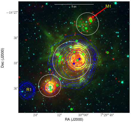
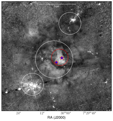
Figure 15: Left panel: Color composite image of Sh 2-305 obtained by using 22 $\mu$m (red), 3.6 $\mu$m (green) $\mu$m and 2.2 $\mu$m (blue) images taken from WISE, $Spitzer$ and 2MASS, respectively. NVSS 1.4 GHz radio continuum contours are shown by blue curves at 10, 20, 30, 40 and 50 % of the peak flux value (0.0145 Jy). Positions of the two previously identified massive stars (O8.5V:VM4 and O9.5:VM2) are shown by blue star symbols. The white circles represent the three sub-clusterings identified in the present analysis. The red circle enclosing the CC is the core region of the central clustering (cf. Section 3.1). Right panel: Spitzer ratio map of 4.5 $\mu$m/3.6 $\mu$m emission. The ratio map is smoothened using a Gaussian function with radius of four pixels.

4.2 MF and KLF slope

The higher-mass stars mostly follow the Salpeter MF (Salpeter, 1955). At lower masses, the IMF is less well constrained, but appears to flatten below 1 M_⊙ and exhibits fewer stars of the lowest masses (Kroupa, 2002; Chabrier, 2003; Luhman et al., 2016). In this study, we find a change of MF slope from the high to low mass end with a turn-off at around 1.5 M_⊙. This truncation of MF slope at a bit higher mass bins has often been noticed in other SFRs also under the influence of massive OB-type stars (Sharma et al., 2007; Pandey et al., 2008; Jose et al., 2008; Sharma et al., 2017). While the higher-mass domain is thought to be mostly formed through fragmentation and/or accretion onto the protostellar core (e.g., Padoan & Nordlund, 2002; Bonnell & Bate, 2006) in the low-mass and substellar regime additional physics is likely to play an important role. The density, velocity fields, chemical composition, tidal forces in the natal molecular clouds, and photo-erosion in the radiation field of massive stars in the vicinity can lead to different star formation processes and consequently some variation in the characteristic mass (turn-off point) of the IMF (Padoan & Nordlund, 2002; Whitworth & Zinnecker, 2004; Bate & Bonnell, 2005; Bate, 2009).

We have also found that the MF slopes are bit steeper ($\Gamma\simeq$-1.7) than the Salpeter (1955) value i.e., $\Gamma$=-1.35 in a mass range of $1.5<M_{\odot}<6.5$, indicating the abundance of low-mass stars, probably formed due to the positive feedback of the massive stars in this region. Most of the sensitive studies of massive SFRs (see, e.g. Liu et al., 2009; Espinoza et al., 2009; Preibisch et al., 2011) found large numbers of low-mass stars in agreement with the expectation from the “normal” field star MF and supports the notion that OB associations and massive star clusters are the dominant supply sources for the Galactic field star population, as already suggested by Miller & Scalo (1978).

The KLF slope value ($\alpha=0.40\pm 0.04$) for the Mayer 3 cluster is similar to the average slopes ($\alpha\sim 0.4$) for embedded clusters (Lada & Lada, 1991, 2003). For north and south sub-clusterings, the KLF slope is lower ($\alpha\simeq 0.2$). Low KLF values (0.27 - 0.31) has been found for some of the very young star clusters (Be 59: Pandey et al. (2008); Stock 8: Jose et al. (2008); W3 Main: Ojha et al. (2004a)). This indicate that the north and south sub-clusterings are bit younger as compared to the central cluster Mayer 3.

4.3 Star formation in the Sh 2-305

Russeil et al. (1995) reported the velocity of H$\alpha$ emission to be 38 km s^-1 in Sh 2-305, which was noticeable different as compared to the radial velocities from CO emission (i.e., $V_{LSR}\sim$43 km s^-1). They suggested that the champagne flow mechanism (Tenorio-Tagle, 1979) might be responsible for this discrepancy between the ionized and molecular material. In this mechanism, if the H ii region is on the near side of the molecular cloud, the ionized gas flows away from the molecular material, more or less in the direction of an observer. Massive stars can influence their surrounding and trigger the formation of new generation of stars, either by sweeping the neighboring molecular gas into a dense shell which subsequently fragments into pre-stellar cores (e.g., Elmegreen & Lada, 1977; Whitworth et al., 1994; Elmegreen, 1998) or by compressing pre-existing dense clumps (e.g., Sandford et al., 1982; Bertoldi, 1989; Lefloch & Lazareff, 1994). The former process is called ‘collect and collapse’ and the later ‘radiation driven implosion’.

There are many examples in literature in which the massive stars have triggered the formation of YSOs in the GMCs (Yadav et al., 2016; Sharma et al., 2017; Das et al., 2017, and references therein). YSOs are mostly found embedded in the GMCs with large variation in their numbers imprinting the fractal structure of the GMCs. Thus, the density variations of the YSOs (i.e., embedded clusters) provide a direct observational signature of the star formation processes. In this study also, we have identified a population of YSOs distributed in the Sh 2-305 in three major clusterings, i.e., the central cluster of YSOs (CC) lies within the boundary of cluster Mayer 3 and other two (NC & SC) in north and south directions at a distance of $\sim$5 pc from the CC. The CC lies in a region with lowest column density, which can be attributed to the dispersion of the gas by two massive stars located in this region (VM2 and VM4, cf. Figure 1). The SC is found to be highly obscured and have the highest value of SFE and the fraction of Class i sources (cf. Table 11), suggesting an active star formation in this core.

To further investigate the influence of massive stars, in the left panel of Figure 15 we show the color composite image of the Sh 2-305 obtained by using 22 $\mu$m (red), 3.6 $\mu$m (green) and 2.2 $\mu$m (blue) images. Spatial distribution of the radio continuum emission (NVSS 1.4 GHz), massive stars, and the YSOs are also shown. This region also has a compact radio source (R1 in the left panel of Figure 15), possibly a young ultra-compact H ii region lying at about $\sim 7^{\prime}$ from the Sh 2-305 center (Fich, 1993; Russeil et al., 1995) and an H₂O maser coinciding with the infrared source IRAS 07277-1821 (M1 in the left panel Figure 15) (Wouterloot et al., 1988). SC and NC appears to host radio continuum emission and H2O maser, respectively, which indicates that high (or massive) stars are forming inside these structures. Though, in general radio counterpart traces more evolved state than H2O maser, but in the present study, it is difficult to differentiate the evolution status of NC and SC considering the errors on the derived parameters. The ionized region (radio continuum emission) and the heated dust grains (22 $\micron$ emission) are distributed towards the CC in the Sh 2-305. The CC is also surrounded by 3.6 $\mu$m emission which covers the prominent PAH features at 3.3 $\mu$m, indicative of photon dominant region (PDR) under the influence of feedback from massive stars (see e.g. Peeters et al., 2004). The massive stars, VM2 and VM4, are located near the center of CC and their high energy feedback might be responsible for these emissions.

The right panel of Figure 15 shows the Spitzer ratio map of 4.5 $\mu$m/3.6 $\mu$m emission, revealing the existence of dark and bright regions. The Spitzer band at 4.5 $\mu$m contains a prominent molecular hydrogen line emission ($\nu$ = 0–0 $S$(9); 4.693 $\mu$m) and the Br-$\alpha$ emission (at 4.05 $\mu$m). The Spitzer band at 3.6 $\mu$m includes the PAH emission at 3.3 $\mu$m. Note that both these Spitzer images have the same PSF, allowing to remove point-like sources as well as continuum emission (see Dewangan et al., 2017, for more details). In the ratio map, the bright regions indicate the excess of 4.5 $\mu$m emission, while the black or dark gray regions show the domination of 3.6 $\mu$m emission. The regions with the excess of 4.5 $\mu$m emission (i.e., bright regions) are seen in the direction of the NVSS radio continuum emission, suggesting the presence of the Br-$\alpha$ emission. Furthermore, the bright regions ($\sim$ $\alpha$₂₀₀₀ =07^h29^m55.7^s, $\delta$₂₀₀₀ = -18$\arcdeg$28$\arcmin$03$\arcsec$) away from the NVSS radio continuum emission appear to trace the outflow activities in the Sh 2-305, where YSOs are also investigated. Considering the PAH feature at 3.3 $\mu$m in the 3.6 $\mu$m band, several dark regions trace the presence of PDRs in the Sh 2-305, indicating the impact of massive O-type stars (i.e., VM2 and VM4). Overall, the Spitzer map displays the signatures of outflow activities and the impact of massive stars in the Sh 2-305. Hence, star formation activities in Sh 2-305 seem to be influenced by massive O-type stars.

To quantify the impact of massive O-type stars (i.e., VM2 and VM4) on their surroundings, we have calculated the total pressure exerted by these two sources (see Section 3.9 and Table 10). The total pressure (P_total) at D_s = 1 pc (Mayer 3 cluster core), 2.4 pc (Mayer 3 cluster extent), 5 pc (location of two YSOs clumps i.e. NC and SC), and 7.5 pc (location of the radio source R1) is 6.4$\times$10^-10, 1.5$\times$10^-10, 4.8$\times$10^-11, and 2.6$\times$10^-11 (dynes  cm^-2), respectively. We have also calculated the P_total at far distance of D_s = 10 pc as 1.6$\times$10^-11 (dynes  cm^-2), which is comparable to the pressure of a typical cool molecular cloud ($P_{MC}$$\sim$10^-11–10^-12 dynes cm^-2 for a temperature $\sim$20 K and particle density $\sim$10³–10⁴ cm^-3) (see Table 7.3 of Dyson & Williams, 1980).

From these calculations, we can easily see that the pressure near massive stars (a core region having CC) is significantly higher as compared to that of a molecular cloud and then it starts to decrease with the distance. At the location of NC and SC, the pressure exerted by ionizing sources is still significant. Also, the YSOs in the NC and SC are found to be younger than that of the CC (cf. Table 11), implying that the star formation there might have started after CC. This is in line to the feedback effects from central massive stars.

Therefore, based on the distribution of warm dust/ionized region near the CC which is surrounded by the PDRs and YSOs, pressure calculations, age gradient etc., we conclude that massive O-type stars associated with the CC might have triggered the formation of younger stars located in the region including NC and SC. This argument is also supported with the slopes of MF/KLF, SFEs, mean age of YSOs, fraction of Class i sources, and dense gas mass, found in these regions.

Regarding the formation of the central massive stars itself along with the origin of radio peak powered by the ultra-compact H ii region, it requires further detailed analysis. It has been observationally reported that the merging/collisions of filamentary structures can form the dense massive star-forming clumps, where the most massive stars form (e.g., Schneider et al., 2012; Nakamura et al., 2014). Identification of embedded filaments and characterizing their physical properties (e.g. temperature and column density, velocity profile, etc) by using high-resolution multiwavelength (from radio to mm, i.e., ionized region, molecular distribution, distribution of cold and warm dust) investigation can help us to explore this scenario as well.

5 Conclusion

In the present work we studied a Galactic H ii region Sh 2-305 to understand the star formation using deep optical and NIR photometry (V$\sim$22 mag, K$\sim$18.1 mag), along with multiwavelength archival data. Following are the conclusions made from the above study.

• Stellar density distribution generated by using NIR data has been used to study the structure of the molecular cloud and clusterings in the Sh 2-305. We have found three stellar sub-clusterings in this region, i.e, one in the central region (Mayer 3) and one each towards north and south directions of the Sh 2-305. One hundred thirty seven cluster members on the basis of Gaia DR2 proper motion data are found to be associated with Mayer 3. These member stars indicate a normal reddening law towards this region. The foreground reddening and distance to the cluster come out to be $E(B-V)$ = 1.17 mag and 3.7 kpc, respectively.

• We identified $\sim$116 YSOs in the $\sim 18^{\prime}.5\times 18^{\prime}.5$ FOV of Sh 2-305 on the basis of excess IR emission. Out of them 87% (96) are Class ii and 13% (20) are Class i sources. Age and mass of 98 YSOs has been estimated using the SED fitting analysis. The masses of the YSOs range between 0.8 to 16.2 M_⊙, however, a majority ($\sim$80%) of them ranges between 0.8 to 4.0 M_⊙ . It is found that $\sim$91% (89/98) of the sources have ages between 0.1 to 3.5 Myr. The region indicates a differential reddening which vary between $A_{V}$=2.2 to 23 mag, indicating a clumpy nature of gas and dust in this region. The average age, mass and $A_{V}$ for this sample of YSOs are 1.8 Myr, 2.9 M_⊙ and 7.1 mag, respectively.

• MST analysis of YSO’s location yields three cores viz. North Clump (NC), Central Clump (CC) and South Clump (SC) which match well with the stellar density distribution. The active region contains 96 YSOs, out of which 74 (77%) belong to these cores. The average MST branch length in these cores is found to be $\sim$0.3 pc.

• Basic structural parameters of these cores have been estimated. The core size and aspect ratio vary between 1.4 - 3 pc and 0.73 - 1.40, respectively. The CC is showing higher YSOs density as compared to other cores. Mean extinction value for the NC, CC and SC is 7.4 mag, 5.9 mag, 10.1 mag, respectively. The molecular mass associated with NC, CC , SC and AR is 379.8 M_⊙, 453.8 M_⊙, 96.1 M_⊙ and 3199.7 M_⊙, respectively. We have found that the SC has the highest value of dense gas mass (55.8 M_⊙), whereas the CC has no dense gas mass associated with it. The Jeans length ‘$\lambda_{J}$’ is calculated as 1.13, 1.35 and 0.83 pc for NC, CC and SC, respectively. SFE has the highest value (36.5 %) for SC, 21.4 % for CC and the lowest value (15.6 %) for NC.

• The slope of the MF, $\Gamma$, in the mass range $1.5<M_{\odot}<6.5$ is found to be $\sim$ -1.7, which is steeper than the Salpeter (1955) value ($\Gamma$=-1.35) and suggests an abundance of low-mass stars, probably formed due to the positive feedback of the massive stars in this region. The KLF slope values for Mayer 3 cluster ($\alpha=0.40\pm 0.04$) and the north and south sub-clusterings ($\alpha\simeq 0.2$) indicate that the north and south sub-clusterings are bit younger as compared to the central cluster Mayer 3.

• It is found that the two massive O-type stars (VM2 and VM4) located in the center of Sh 2-305 might have triggered the formation of younger stars. This argument is also supported with the distribution of warm dust/ionized region surrounded by the PDRs and YSOs, pressure calculations, age gradient, slopes of MF/KLF, SFEs, mean age of YSOs, fraction of Class i sources, and dense gas mass, for the sub-clusterings found in the region.

Table 1: Log of observations.

Telescope/Instrument	Comments	Exp. (sec)$\times$ No. of frames
$[$Date of observations$]$	$[$Filter$]$
1.3 m DFOT/2K CCD	Optical imaging of Sh 2-305
$[$ 2014 Jan 29$]$	$U$	$300\times 4$
$"$	$B$	$300\times 3,30\times 3$
$"$	$V$	$300\times 3,60\times 3,10\times 3$
$"$	$R_{c}$	$300\times 3,60\times 3,10\times 3$
$"$	$I_{c}$	$300\times 3,60\times 3,10\times 3$
$[$2017 Mar 19 $]$	$I_{c}$	$1800\times 4$
$[$2017 Mar 23$]$	$V$	$1800\times 2$
	Optical imaging of Standard field (SA98)
$[$2014 Jan 29$]$	$U$	$300\times 5,120\times 1$
$"$	$B$	$120\times 2,40\times 3,60\times 1$
$"$	$V$	$30\times 3,60\times 3$
$"$	$R_{c}$	$30\times 3,20\times 3$
$"$	$I_{c}$	$30\times 3,20\times 3$
2m HCT/TIRSPEC	NIR imaging of Sh 2-305 (five pointings)
$[$2016 Feb 1 & 2017 Oct 9$]$	$J$	$20\times 35$
$"$	$H$	$20\times 35$
$"$	$K$	$20\times 35$

Table 2: Completeness of the photometric data

Band	Number of	Detection	Completeness	Completeness Limit (up to 80 %)
	sources	Limit (mag)	Limit (up 80 %) (mag)	Mass ($M_{\odot}$c)
$U$	712	20.0	$-$	$-$
$B$	1249	20.9	$-$	$-$
$V$	2646	21.9	20.5	0.7
$R_{c}$	2467	20.9	$-$	$-$
$I_{c}$	2641	20.0	22.0	0.1
$J$	1062a+ 1104b	19.2	17.0	0.7
$H$	1796a+ 1134b	18.7	16.0	0.8
$K$	1796a+ 1134b	18.1	15.5	1.1
$[3.6]$	2246	16.3	14.2	1.4
$[4.5]$	2246	15.7	13.5	1.5

^a: data from $TIRSPEC$; ^b: data from 2MASS; ^c: for distance = 3.7 kpc and $E(B-V)$ = 1.17 mag.

Table 3: Sample of 137 stars identified as a member of the Sh 2-305. The complete table is available in the electronic form only.

ID	$\alpha_{(2000)}$	$\delta_{(2000)}$	Parallax$\pm\sigma~{}~{}~{}~{}~{}$	$\mu_{\alpha}\pm\sigma$	$\mu_{\delta}\pm\sigma$	$G$	$G_{BP}-G_{RP}$	Probability
	$(degrees)$	$(degrees)$	(mas)	(mas/yr)	(mas/yr)	(mag)	(mag)	(Percentage)
1	112.506538	-18.626102	$0.108\pm 0.500$	$-1.759\pm 0.591$	$1.351\pm 0.805$	$19.979$	2.700	81
2	112.543953	-18.622734	$0.082\pm 0.113$	$-1.769\pm 0.128$	$2.049\pm 0.166$	$17.645$	1.569	98
3	112.491783	-18.620470	$0.866\pm 0.247$	$-1.729\pm 0.294$	$1.907\pm 0.352$	$18.883$	1.977	95
4	112.505150	-18.618370	$0.198\pm 0.545$	$-1.536\pm 0.618$	$2.235\pm 0.741$	$20.075$	1.849	89

Table 4: A sample table containing information for 116 YSOs identified in the Sh 2-305. The complete table is available in an electronic form only.

ID	$\alpha_{(2000)}$	$\delta_{(2000)}$	$J\pm\sigma$	$H\pm\sigma$	$K\pm\sigma$	$[3.6]\pm\sigma$	$[4.5]\pm\sigma$	$[3.4]\pm\sigma$	$[4.6]\pm\sigma$	$[12]\pm\sigma$	$[22]\pm\sigma$	Class
	$(degrees)$	$(degrees)$	(mag)	(mag)	(mag)	(mag)	(mag)	(mag)	(mag)	(mag)	(mag)
1	112.539932	-18.666079	$-$	$15.787\pm 0.171$	$14.997\pm 0.150$	$13.843\pm 0.082$	$13.189\pm 0.051$	$13.837\pm 0.026$	$12.933\pm 0.029$	$-$	$-$	II
2	112.639084	-18.660336	$12.038\pm 0.027$	$11.469\pm 0.034$	$10.863\pm 0.024$	$9.555\pm 0.109$	$9.033\pm 0.079$	$9.623\pm 0.022$	$8.912\pm 0.018$	$5.412\pm 0.012$	$3.68\pm 0.024$	II
3	112.524623	-18.640574	$-$	$15.332\pm 0.130$	$14.344\pm 0.092$	$12.871\pm 0.059$	$12.016\pm 0.048$	$12.309\pm 0.022$	$11.024\pm 0.021$	$8.505\pm 0.081$	$5.862\pm 0.047$	I
4	112.529347	-18.621298	$-$	$15.837\pm 0.176$	$14.785\pm 0.112$	$14.013\pm 0.089$	$13.362\pm 0.044$	$13.699\pm 0.054$	$12.632\pm 0.050$	$-$	$5.883\pm 0.170$	II

Table 5: A sample table containing information for 28 optically identified YSOs. IDs are the same as in Table 4. The complete table is available in an electronic form only.

ID	$V\pm\sigma$	$(U-B)\pm\sigma$	$(B-V)\pm\sigma$	$(V-R_{c})\pm\sigma$	$(V-I_{c})\pm\sigma$
	(mag)	(mag)	(mag)	(mag)	(mag)
$2$	$14.534\pm 0.003$	$0.382\pm 0.013$	$1.047\pm 0.009$	$0.541\pm 0.004$	$1.280\pm 0.005$
$7$	$17.699\pm 0.007$	$-$	$1.737\pm 0.019$	$0.976\pm 0.011$	$2.142\pm 0.011$
$11$	$17.821\pm 0.047$	$-0.222\pm 0.170$	$2.089\pm 0.056$	$1.769\pm 0.063$	$3.237\pm 0.076$
$16$	$15.555\pm 0.004$	$0.233\pm 0.018$	$0.963\pm 0.009$	$0.475\pm 0.017$	$1.272\pm 0.012$

Table 6: A sample table containing stellar parameters of selected 98 YSOs derived using the SED fitting analysis. IDs are the same as in Table 4. The complete table is available in an electronic form only.

ID	$N_{data}$	$\chi^{2}_{min}$	$A_{V}$$\pm\sigma$	Age$\pm\sigma$	Mass$\pm\sigma$
			(mag)	(Myr)	($M_{\odot}$)
1	9	2.2	$6.2\pm 3.8$	$0.4\pm 1.2$	$0.8\pm 0.8$
2	14	19.1	$2.7\pm 0.3$	$0.6\pm 0.1$	$4.9\pm 0.3$
4	9	11.0	$5.0\pm 3.6$	$0.6\pm 1.6$	$1.6\pm 1.4$
6	5	0.4	$9.6\pm 3.1$	$1.7\pm 2.5$	$3.0\pm 1.2$

Table 7: The values of mass function (MF) and $K$-band luminosity function (KLF) slopes for the stellar sub-clusterings identified in the Sh 2-305 (cf. Section 3.1).

Region	MF Slope	KLF Slope
	($\Gamma$)	$(\alpha)$
North sub-clustering	$-$	$0.24\pm 0.14$
Mayer 3	$-1.69\pm 0.49$	$0.40\pm 0.04$
South sub-clustering	$-1.78\pm 0.48$	$0.21\pm 0.04$
Whole region	$-1.76\pm 0.30$	$0.33\pm 0.04$

Table 8: Properties of the clumps identified using the Herschel column density map. Center coordinates of the identified clumps along with the radius (column 4) and mass (column 5) of the clumps are given in the table.

ID	$\alpha_{(2000)}$	$\delta_{(2000)}$	Radius	Mass
	$(^{h}:^{m}:^{s})$	$(^{o}:^{\prime}:^{\prime\prime)}$	(pc)	(M⊙)
1	07:29:43.1	-18:24:15	0.42	85
2	07:29:57.0	-18:28:03	1.32	1565
3	07:29:59.1	-18:29:03	0.81	410
4	07:30:05.9	-18:28:33	0.60	175
5	07:30:05.5	-18:30:51	0.91	700
6	07:30:01.2	-18:31:57	0.66	320
7	07:29:53.2	-18:32:03	0.28	35
8	07:29:44.8	-18:32:09	0.79	355
9	07:29:35.9	-18:33:57	0.85	415
10	07:30:32.0	-18:30:57	0.53	140
11	07:30:13.9	-18:30:33	0.77	335
12	07:30:16.8	-18:31:27	0.84	465
13	07:30:13.9	-18:32:15	0.96	845
14	07:30:07.6	-18:32:57	0.40	85
15	07:30:10.5	-18:34:09	0.33	50
16	07:30:01.2	-18:33:39	0.69	305
17	07:30:01.7	-18:34:51	0.64	270
18	07:30:05.9	-18:35:27	0.40	80
19	07:30:07.6	-18:35:39	0.55	145
20	07:30:16.8	-18:36:03	1.00	715
21	07:30:24.4	-18:37:03	0.33	50
22	07:30:27.4	-18:38:57	0.32	45
23	07:30:06.7	-18:37:33	1.25	930
24	07:30:06.7	-18:38:33	1.05	670
25	07:30:10.1	-18:40:03	0.90	415

Table 9: Properties of the identified cores and ARs. Center coordinates of the identified cores and ARs along with the total number of the YSOs are given in columns 2, 3 and 4, respectively. The vertices of the convex hull, hull radius and circle radius along with the aspect ratio are given in columns 5, 6, 7 and 8, respectively. Columns 9 and 10 represent the mean and peak stellar density obtained using the isodensity contours. Columns 11, 12 and 13 are the mean MST branch length, NN distances and $Q$ parameters, respectively.

Region	$\alpha_{(2000)}$	$\delta_{(2000)}$	Na	Vb	$R_{\rm hull}$	$R_{\rm cir}$	Aspect	$\sigma_{\rm mean}$	$\sigma_{\rm peak}$	MSTc	NN2c	$Q$
	$(^{h}:^{m}:^{s})$	$(^{o}:^{\prime}:^{\prime\prime)}$			(pc)	(pc)	Ratio	(pc-2)	(pc-2)	(pc)	(pc)
NC	07:29:58.14	-18:28:07.9	22	7	1.26	1.48	1.40	4.44	21.9	0.39	0.32	0.72
CC	07:30:06.22	-18:32:32.5	44	11	1.54	1.59	1.07	5.94	31.3	0.26	0.18	0.66
SC	07:30:18.06	-18:35:49.6	8	5	0.71	0.61	0.73	5.08	11.1	0.28	0.27	0.84
AR	07:30:06.05	-18:31:53.5	96	12	3.48	5.77	2.76	2.53	31.3	0.33	0.25	0.56

a: Number of YSOs enclosed in the group; b: Vertices of the convex hull; c: median branch length;

Table 10: Combined pressure components driven by two massive stars (i.e., O8.5V and O9.5V) at different D_s (cf. Section 3.9) .

Pressure	Ds = 1 pc	Ds = 2.4 pc	Ds = 5 pc	Ds = 7.5 pc	Ds = 10 pc
(dynes  cm-2)
PHII	4.6$\times$10-10	1.2$\times$10-10	4.1$\times$10-11	2.3$\times$10-11	1.4$\times$10-11
Prad	1.7$\times$10-10	3.0$\times$10-11	6.8$\times$10-12	3.0$\times$10-12	1.7$\times$10-12
Pwind	2.6$\times$10-12	4.7$\times$10-13	1.1$\times$10-13	4.8$\times$10-14	2.7$\times$10-14
Ptotal	6.4$\times$10-10	1.5$\times$10-10	4.8$\times$10-11	2.6$\times$10-11	1.6$\times$10-11

Table 11: Properties of the identified cores and ARs. Columns 2, 3, 4 represent the Jeans length, ratio of Jeans length with mean separation of YSOs, and star formation efficiency (SFE), respectively. The mean and peak extinction values are given in columns 5 and 6, respectively. Column 7 represents the cloud mass in the convex hull derived using the extinction maps. Column 8 represents the mass of the dense gas having $A_{K}$ greater than 0.8 mag. Columns 9, 10 and 11 represent the number of Class i, Class ii YSOs along with the fraction of Class i YSOs over total YSOs. Columns 12, 13 and 14 represent the mean age and mean mass, derived from the SED analysis along with the number of YSOs used in that analysis.

Region	$\lambda_{J}$	$\lambda_{J}$/$S_{YSO}$	SFE	$A_{V_{mean}}^{d}$	$A_{V_{peak}}$	Mass	Mass0.8	Class	Class	Frace	Age	Mass	N
	(pc)		(%)	(mag)	(mag)	(M⊙)	(M⊙)	(I)	(II)	$(\%)$	(Myr)	(M⊙)	(SED)
NC	$1.13\pm 0.22$	3.4	$15.6\pm 4$	$7.4\pm 1.5$	12.0	$379.8\pm 81$	$17.8\pm 2$	4	18	18	$1.7\pm 1.2$	$3.2\pm 1.6$	19
CC	$1.35\pm 0.27$	5.2	$21.4\pm 5$	$5.9\pm 1.4$	10.5	$453.8\pm 97$	-	7	37	16	$1.8\pm 1.2$	$2.8\pm 1.6$	39
SC	$0.83\pm 0.16$	2.5	$36.5\pm 6$	$10.1\pm 1.4$	14.0	$96.1\pm 17$	$55.8\pm 8$	2	6	25	$1.2\pm 0.9$	$6.9\pm 4.7$	5
AR	$1.86\pm 0.34$	4.7	$8.5\pm 5$	$6.7\pm 1.6$	17.9	$3199.7\pm 800$	$219.3\pm 30$	18	78	19	$1.7\pm 1.2$	$3.1\pm 2.2$	78

d = from NIR+2MASS $(H-K)$ map; e: Class i/(Class i + Class ii)

Appendix A Reddening Law

We have used the technique as described by Pandey et al. (2003) to study the nature of the diffuse interstellar medium (ISM) associated with the Sh 2-305 region. This can be represented by the ratio of total-to-selective extinction $R_{V}$ = $A_{V}$/$E(B-V)$. Though in the solar neighborhood, the normal reddening law gives the value $R_{V}$ = 3.1$\pm$ 0.2 (Whittet, 2003; Guetter & Vrba, 1989; Lim et al., 2011), in the case of several SFRs, it is found to be anomalously high (see e.g., Pandey et al., 2000, 2008; Hur et al., 2012; Pandey et al., 2013; Kumar et al., 2014). The two-color diagrams (TCDs) of the form of $(V-\lambda)$ versus $(B-V)$, where $\lambda$ indicates one of the wavelengths of the broad-band filters ($R,I,J,H,K,L$), provide an effective method for separating the influence of the normal extinction produced by the general ISM from that of the abnormal extinction arising within regions having a peculiar distribution of dust sizes (cf. Chini et al., 1990; Pandey et al., 2000). We have selected all member stars of Sh 2-305 having optical and NIR detections and plotted their $(V-\lambda)$ versus $(B-V)$ TCDs in Figure 16. Since YSOs show excess infra-red (IR) emission, their positions can deviate from those of the MS stars in the TCDs, therefore they have not been used in the calculation of the reddening law. The slopes of the least squares fit to the distribution of the MS member stars (black dots) in the $(V-I_{c}),(V-J),(V-H)$ and $(V-K)$ versus $(B-V)$ TCDs are found to be $1.20\pm 0.07,2.14\pm 0.16,2.51\pm 0.18$ and $2.67\pm 0.21$, respectively, which are within error similar to those found for the general ISM (1.10, 1.96, 2.42 and 2.60; cf., Pandey et al., 2003), indicating normal reddening law ‘$R_{V}$ = 3.1’ in this region.

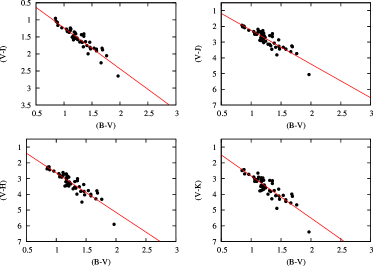
Figure 16: $(V-I_{c}),(V-J),(V-H),(V-K)$ vs. $(B-V)$ TCDs for the stars associated with the Sh 2-305 region. Straight lines show the least-square fit to the distribution of stars.

References

- Allen et al. (2007) Allen, L., Megeath, S. T., Gutermuth, R., et al. 2007, Protostars and Planets V, 361
- Allen et al. (2008) Allen, T. S., Pipher, J. L., Gutermuth, R. A., et al. 2008, ApJ, 675, 491, doi: 10.1086/525241
- Alves et al. (2007) Alves, J., Lombardi, M., & Lada, C. J. 2007, A&A, 462, L17, doi: 10.1051/0004-6361:20066389
- André et al. (2010) André, P., Men’shchikov, A., Bontemps, S., & et. al, . 2010, A&A, 518, L102, doi: 10.1051/0004-6361/201014666
- Azimlu & Fich (2011) Azimlu, M., & Fich, M. 2011, AJ, 141, 123, doi: 10.1088/0004-6256/141/4/123
- Bailer-Jones et al. (2018) Bailer-Jones, C. A. L., Rybizki, J., Fouesneau, M., Mantelet, G., & Andrae, R. 2018, AJ, 156, 58, doi: 10.3847/1538-3881/aacb21
- Bastian (2010) Bastian, N. 2010, in From Stars to Galaxies: Connecting our Understanding of Star and Galaxy Formation, 128
- Bastian et al. (2007) Bastian, N., Ercolano, B., Gieles, M., et al. 2007, MNRAS, 379, 1302, doi: 10.1111/j.1365-2966.2007.12064.x
- Bastian et al. (2009) Bastian, N., Gieles, M., Ercolano, B., & Gutermuth, R. 2009, MNRAS, 392, 868, doi: 10.1111/j.1365-2966.2008.14107.x
- Bate (2009) Bate, M. R. 2009, MNRAS, 392, 1363, doi: 10.1111/j.1365-2966.2008.14165.x
- Bate & Bonnell (2005) Bate, M. R., & Bonnell, I. A. 2005, MNRAS, 356, 1201, doi: 10.1111/j.1365-2966.2004.08593.x
- Bertoldi (1989) Bertoldi, F. 1989, ApJ, 346, 735, doi: 10.1086/168055
- Bessell & Brett (1988) Bessell, M. S., & Brett, J. M. 1988, PASP, 100, 1134, doi: 10.1086/132281
- Bica et al. (2003) Bica, E., Dutra, C. M., & Barbuy, B. 2003, A&A, 397, 177, doi: 10.1051/0004-6361:20021479
- Bisbas et al. (2009) Bisbas, T. G., Wünsch, R., Whitworth, A. P., & Hubber, D. A. 2009, A&A, 497, 649, doi: 10.1051/0004-6361/200811522
- Bonnell & Bate (2006) Bonnell, I. A., & Bate, M. R. 2006, MNRAS, 370, 488, doi: 10.1111/j.1365-2966.2006.10495.x
- Bressert et al. (2012) Bressert, E., Ginsburg, A., Bally, J., et al. 2012, ApJ, 758, L28, doi: 10.1088/2041-8205/758/2/L28
- Cardelli et al. (1989) Cardelli, J. A., Clayton, G. C., & Mathis, J. S. 1989, ApJ, 345, 245, doi: 10.1086/167900
- Cartwright & Whitworth (2004) Cartwright, A., & Whitworth, A. P. 2004, MNRAS, 348, 589, doi: 10.1111/j.1365-2966.2004.07360.x
- Chabrier (2003) Chabrier, G. 2003, PASP, 115, 763, doi: 10.1086/376392
- Chauhan et al. (2011) Chauhan, N., Pandey, A. K., Ogura, K., et al. 2011, MNRAS, 415, 1202, doi: 10.1111/j.1365-2966.2011.18742.x
- Chauhan et al. (2009) —. 2009, MNRAS, 396, 964, doi: 10.1111/j.1365-2966.2009.14756.x
- Chavarría et al. (2014) Chavarría, L., Allen, L., Brunt, C., et al. 2014, MNRAS, 439, 3719, doi: 10.1093/mnras/stu224
- Chen et al. (2004) Chen, W. P., Chen, C. W., & Shu, C. G. 2004, AJ, 128, 2306, doi: 10.1086/424855
- Chini et al. (1990) Chini, R., Kruegel, E., & Kreysa, E. 1990, A&A, 227, L5
- Chini & Wink (1984) Chini, R., & Wink, J. E. 1984, A&A, 139, L5
- Cohen et al. (1981) Cohen, J. G., Persson, S. E., Elias, J. H., & Frogel, J. A. 1981, ApJ, 249, 481, doi: 10.1086/159308
- Cutri et al. (2003) Cutri, R. M., Skrutskie, M. F., van Dyk, S., et al. 2003, VizieR Online Data Catalog, 2246, 0
- Das et al. (2017) Das, S. R., Tej, A., Vig, S., et al. 2017, MNRAS, 472, 4750, doi: 10.1093/mnras/stx2290
- Dewangan et al. (2017) Dewangan, L. K., Ojha, D. K., Zinchenko, I., Janardhan, P., & Luna, A. 2017, ApJ, 834, 22, doi: 10.3847/1538-4357/834/1/22
- Dickman (1978) Dickman, R. L. 1978, ApJS, 37, 407, doi: 10.1086/190535
- Dutra et al. (2003) Dutra, C. M., Bica, E., Soares, J., & Barbuy, B. 2003, A&A, 400, 533, doi: 10.1051/0004-6361:20030005
- Dyson & Williams (1980) Dyson, J. E., & Williams, D. A. 1980, Physics of the interstellar medium
- Efremov (1978) Efremov, Y. N. 1978, Pisma v Astronomicheskii Zhurnal, 4, 125
- Elmegreen (1998) Elmegreen, B. G. 1998, in Astronomical Society of the Pacific Conference Series, Vol. 148, Origins, ed. C. E. Woodward, J. M. Shull, & H. A. Thronson, Jr., 150
- Elmegreen & Falgarone (1996) Elmegreen, B. G., & Falgarone, E. 1996, ApJ, 471, 816, doi: 10.1086/178009
- Elmegreen & Lada (1977) Elmegreen, B. G., & Lada, C. J. 1977, ApJ, 214, 725, doi: 10.1086/155302
- Espinoza et al. (2009) Espinoza, P., Selman, F. J., & Melnick, J. 2009, A&A, 501, 563, doi: 10.1051/0004-6361/20078597
- Evans et al. (2009) Evans, II, N. J., Dunham, M. M., Jørgensen, J. K., et al. 2009, ApJS, 181, 321, doi: 10.1088/0067-0049/181/2/321
- Fall et al. (2010) Fall, S. M., Krumholz, M. R., & Matzner, C. D. 2010, ApJ, 710, L142, doi: 10.1088/2041-8205/710/2/L142
- Fich (1993) Fich, M. 1993, ApJS, 86, 475, doi: 10.1086/191787
- Flaherty et al. (2007) Flaherty, K. M., Pipher, J. L., Megeath, S. T., et al. 2007, ApJ, 663, 1069, doi: 10.1086/518411
- Girard et al. (1989) Girard, T. M., Grundy, W. M., Lopez, C. E., & van Altena, W. F. 1989, AJ, 98, 227, doi: 10.1086/115139
- Grasha et al. (2017) Grasha, K., Elmegreen, B. G., Calzetti, D., et al. 2017, ApJ, 842, 25, doi: 10.3847/1538-4357/aa740b
- Grasha et al. (2018) Grasha, K., Calzetti, D., Bittle, L., et al. 2018, MNRAS, 481, 1016, doi: 10.1093/mnras/sty2154
- Guetter & Vrba (1989) Guetter, H. H., & Vrba, F. J. 1989, AJ, 98, 611, doi: 10.1086/115161
- Gutermuth et al. (2009) Gutermuth, R. A., Megeath, S. T., Myers, P. C., et al. 2009, ApJS, 184, 18, doi: 10.1088/0067-0049/184/1/18
- Gutermuth et al. (2005) Gutermuth, R. A., Megeath, S. T., Pipher, J. L., et al. 2005, ApJ, 632, 397, doi: 10.1086/432460
- Gutermuth et al. (2011) Gutermuth, R. A., Pipher, J. L., Megeath, S. T., et al. 2011, ApJ, 739, 84, doi: 10.1088/0004-637X/739/2/84
- Gutermuth et al. (2008) Gutermuth, R. A., Myers, P. C., Megeath, S. T., et al. 2008, ApJ, 674, 336, doi: 10.1086/524722
- Hillenbrand (2002) Hillenbrand, L. A. 2002, ArXiv Astrophysics e-prints
- Hillenbrand et al. (2008) Hillenbrand, L. A., Bauermeister, A., & White, R. J. 2008, in Astronomical Society of the Pacific Conference Series, Vol. 384, 14th Cambridge Workshop on Cool Stars, Stellar Systems, and the Sun, ed. G. van Belle, 200
- Hoffman et al. (1983) Hoffman, G. L., Salpeter, E. E., & Wasserman, I. 1983, ApJ, 268, 527, doi: 10.1086/160976
- Hur et al. (2012) Hur, H., Sung, H., & Bessell, M. S. 2012, AJ, 143, 41, doi: 10.1088/0004-6256/143/2/41
- Indebetouw et al. (2005) Indebetouw, R., Mathis, J. S., Babler, B. L., & et. al, . 2005, ApJ, 619, 931, doi: 10.1086/426679
- Jose et al. (2016) Jose, J., Kim, J. S., Herczeg, G. J., et al. 2016, ApJ, 822, 49, doi: 10.3847/0004-637X/822/1/49
- Jose et al. (2008) Jose, J., Pandey, A. K., Ojha, D. K., et al. 2008, MNRAS, 384, 1675, doi: 10.1111/j.1365-2966.2007.12825.x
- Jose et al. (2013) Jose, J., Pandey, A. K., Samal, M. R., et al. 2013, MNRAS, 432, 3445, doi: 10.1093/mnras/stt700
- Kharchenko et al. (2016) Kharchenko, N. V., Piskunov, A. E., Schilbach, E., Röser, S., & Scholz, R.-D. 2016, A&A, 585, A101, doi: 10.1051/0004-6361/201527292
- Kim et al. (2018) Kim, J.-G., Kim, W.-T., & Ostriker, E. C. 2018, ApJ, 859, 68, doi: 10.3847/1538-4357/aabe27
- Koenig et al. (2008) Koenig, X. P., Allen, L. E., Gutermuth, R. A., et al. 2008, ApJ, 688, 1142, doi: 10.1086/592322
- Koenig & Leisawitz (2014) Koenig, X. P., & Leisawitz, D. T. 2014, ApJ, 791, 131, doi: 10.1088/0004-637X/791/2/131
- Kroupa (2002) Kroupa, P. 2002, Science, 295, 82, doi: 10.1126/science.1067524
- Krumholz et al. (2014) Krumholz, M. R., Bate, M. R., Arce, H. G., et al. 2014, in Protostars and Planets VI, ed. H. Beuther, R. S. Klessen, C. P. Dullemond, & T. Henning, 243
- Kuhn et al. (2014) Kuhn, M. A., Feigelson, E. D., Getman, K. V., et al. 2014, ApJ, 787, 107, doi: 10.1088/0004-637X/787/2/107
- Kumar et al. (2014) Kumar, B., Sharma, S., Manfroid, J., et al. 2014, A&A, 567, A109, doi: 10.1051/0004-6361/201323027
- Kwan (1997) Kwan, J. 1997, ApJ, 489, 284, doi: 10.1086/304773
- Lada & Lada (1991) Lada, C. J., & Lada, E. A. 1991, in Astronomical Society of the Pacific Conference Series, Vol. 13, The Formation and Evolution of Star Clusters, ed. K. Janes, 3–22
- Lada & Lada (2003) Lada, C. J., & Lada, E. A. 2003, ARA&A, 41, 57, doi: 10.1146/annurev.astro.41.011802.094844
- Lada et al. (1993) Lada, C. J., Young, E. T., & Greene, T. P. 1993, ApJ, 408, 471, doi: 10.1086/172605
- Landolt (1992) Landolt, A. U. 1992, AJ, 104, 340, doi: 10.1086/116242
- Larson (2007) Larson, R. B. 2007, Reports on Progress in Physics, 70, 337, doi: 10.1088/0034-4885/70/3/R01
- Lefloch & Lazareff (1994) Lefloch, B., & Lazareff, B. 1994, A&A, 289, 559
- Lim et al. (2011) Lim, B., Sung, H. S., Karimov, R., & Ibrahimov, M. 2011, Journal of Korean Astronomical Society, 44, 39. https://arxiv.org/abs/1103.4927
- Liu et al. (2009) Liu, Q., de Grijs, R., Deng, L. C., et al. 2009, MNRAS, 396, 1665, doi: 10.1111/j.1365-2966.2009.14838.x
- Luhman et al. (2016) Luhman, K. L., Esplin, T. L., & Loutrel, N. P. 2016, ApJ, 827, 52, doi: 10.3847/0004-637X/827/1/52
- Mallick et al. (2014) Mallick, K. K., Ojha, D. K., Tamura, M., et al. 2014, MNRAS, 443, 3218, doi: 10.1093/mnras/stu1396
- Marcolino et al. (2009) Marcolino, W. L. F., Bouret, J.-C., Martins, F., et al. 2009, A&A, 498, 837, doi: 10.1051/0004-6361/200811289
- Marigo et al. (2008) Marigo, P., Girardi, L., Bressan, A., et al. 2008, A&A, 482, 883, doi: 10.1051/0004-6361:20078467
- Marsh et al. (2015) Marsh, K. A., Whitworth, A. P., & Lomax, O. 2015, MNRAS, 454, 4282, doi: 10.1093/mnras/stv2248
- Marsh et al. (2017) Marsh, K. A., Whitworth, A. P., Lomax, O., et al. 2017, MNRAS, 471, 2730, doi: 10.1093/mnras/stx1723
- Martins & Palacios (2017) Martins, F., & Palacios, A. 2017, A&A, 598, A56, doi: 10.1051/0004-6361/201629538
- Meyer et al. (1997) Meyer, M. R., Calvet, N., & Hillenbrand, L. A. 1997, AJ, 114, 288, doi: 10.1086/118474
- Miller & Scalo (1978) Miller, G. E., & Scalo, J. M. 1978, PASP, 90, 506, doi: 10.1086/130373
- Molinari et al. (2010a) Molinari, S., Swinyard, B., Bally, J., et al. 2010a, A&A, 518, L100, doi: 10.1051/0004-6361/201014659
- Molinari et al. (2010b) —. 2010b, PASP, 122, 314, doi: 10.1086/651314
- Nakamura et al. (2014) Nakamura, F., Sugitani, K., Tanaka, T., et al. 2014, ApJ, 791, L23, doi: 10.1088/2041-8205/791/2/L23
- Ninan et al. (2014) Ninan, J. P., Ojha, D. K., Ghosh, S. K., et al. 2014, Journal of Astronomical Instrumentation, 3, 1450006, doi: 10.1142/S2251171714500068
- Offner & Arce (2014) Offner, S. S. R., & Arce, H. G. 2014, ApJ, 784, 61, doi: 10.1088/0004-637X/784/1/61
- Ojha et al. (2004a) Ojha, D. K., Tamura, M., Nakajima, Y., et al. 2004a, ApJ, 608, 797, doi: 10.1086/420876
- Ojha et al. (2004b) —. 2004b, ApJ, 616, 1042, doi: 10.1086/425068
- Padoan & Nordlund (2002) Padoan, P., & Nordlund, Å. 2002, ApJ, 576, 870, doi: 10.1086/341790
- Panagia (1973) Panagia, N. 1973, AJ, 78, 929, doi: 10.1086/111498
- Pandey et al. (2000) Pandey, A. K., Ogura, K., & Sekiguchi, K. 2000, PASJ, 52, 847
- Pandey et al. (2019) Pandey, A. K., Sharma, S., Kobayashi, N., Sarugaku, Y., & Ogura, K. 2019, MNRAS, 3221, doi: 10.1093/mnras/stz3596
- Pandey et al. (2008) Pandey, A. K., Sharma, S., Ogura, K., et al. 2008, MNRAS, 383, 1241, doi: 10.1111/j.1365-2966.2007.12641.x
- Pandey et al. (2003) Pandey, A. K., Upadhyay, K., Nakada, Y., & Ogura, K. 2003, A&A, 397, 191, doi: 10.1051/0004-6361:20021509
- Pandey et al. (2013) Pandey, A. K., Eswaraiah, C., Sharma, S., et al. 2013, ApJ, 764, 172, doi: 10.1088/0004-637X/764/2/172
- Panwar et al. (2014) Panwar, N., Chen, W. P., Pandey, A. K., et al. 2014, MNRAS, 443, 1614, doi: 10.1093/mnras/stu1244
- Panwar et al. (2017) Panwar, N., Samal, M. R., Pandey, A. K., et al. 2017, MNRAS, 468, 2684, doi: 10.1093/mnras/stx616
- Peeters et al. (2004) Peeters, E., Spoon, H. W. W., & Tielens, A. G. G. M. 2004, ApJ, 613, 986, doi: 10.1086/423237
- Phelps & Janes (1994) Phelps, R. L., & Janes, K. A. 1994, ApJS, 90, 31, doi: 10.1086/191857
- Pismis & Mampaso (1991) Pismis, P., & Mampaso, A. 1991, MNRAS, 249, 385, doi: 10.1093/mnras/249.3.385
- Preibisch et al. (2011) Preibisch, T., Ratzka, T., Kuderna, B., et al. 2011, A&A, 530, A34, doi: 10.1051/0004-6361/201116781
- Reach et al. (2006) Reach, W. T., Rho, J., Tappe, A., et al. 2006, AJ, 131, 1479, doi: 10.1086/499306
- Robin et al. (2003) Robin, A. C., Reylé, C., Derrière, S., & Picaud, S. 2003, A&A, 409, 523, doi: 10.1051/0004-6361:20031117
- Robitaille et al. (2007) Robitaille, T. P., Whitney, B. A., Indebetouw, R., & Wood, K. 2007, ApJS, 169, 328, doi: 10.1086/512039
- Robitaille et al. (2006) Robitaille, T. P., Whitney, B. A., Indebetouw, R., Wood, K., & Denzmore, P. 2006, ApJS, 167, 256, doi: 10.1086/508424
- Russeil et al. (1995) Russeil, D., Georgelin, Y. M., Georgelin, Y. P., Le Coarer, E., & Marcelin, M. 1995, A&AS, 114, 557
- Salpeter (1955) Salpeter, E. E. 1955, ApJ, 121, 161, doi: 10.1086/145971
- Samal et al. (2012) Samal, M. R., Pandey, A. K., Ojha, D. K., et al. 2012, ApJ, 755, 20, doi: 10.1088/0004-637X/755/1/20
- Sanchawala et al. (2007) Sanchawala, K., Chen, W.-P., Ojha, D., et al. 2007, ApJ, 667, 963, doi: 10.1086/521044
- Sánchez et al. (2010) Sánchez, N., Añez, N., Alfaro, E. J., & Crone Odekon, M. 2010, ApJ, 720, 541, doi: 10.1088/0004-637X/720/1/541
- Sandford et al. (1982) Sandford, II, M. T., Whitaker, R. W., & Klein, R. I. 1982, ApJ, 260, 183, doi: 10.1086/160245
- Scalo (1986) Scalo, J. M. 1986, Fund. Cosmic Phys., 11, 1
- Schmeja & Klessen (2006) Schmeja, S., & Klessen, R. S. 2006, A&A, 449, 151, doi: 10.1051/0004-6361:20054464
- Schmeja et al. (2008) Schmeja, S., Kumar, M. S. N., & Ferreira, B. 2008, MNRAS, 389, 1209, doi: 10.1111/j.1365-2966.2008.13442.x
- Schmidt-Kaler (1982) Schmidt-Kaler, T. 1982, in Landolt-Börnstein: Numerical Data and Functional Relationship in Science and Technology, Vol. 2b. eds. Schaifers K., Voigt H. H., Landolt H. (Springer-Verlag), Berlin, p. 19, ed. V. H. H. L. H. Schaifers, K.
- Schneider et al. (2012) Schneider, N., Csengeri, T., Hennemann, M., et al. 2012, A&A, 540, L11, doi: 10.1051/0004-6361/201118566
- Sharma et al. (2008) Sharma, S., Pandey, A. K., Ogura, K., et al. 2008, AJ, 135, 1934, doi: 10.1088/0004-6256/135/5/1934
- Sharma et al. (2006) —. 2006, AJ, 132, 1669, doi: 10.1086/507094
- Sharma et al. (2017) Sharma, S., Pandey, A. K., Ojha, D. K., et al. 2017, MNRAS, 467, 2943, doi: 10.1093/mnras/stx014
- Sharma et al. (2007) —. 2007, MNRAS, 380, 1141, doi: 10.1111/j.1365-2966.2007.12156.x
- Sharma et al. (2012) Sharma, S., Pandey, A. K., Pandey, J. C., et al. 2012, PASJ, 64, 107. https://arxiv.org/abs/1204.2897
- Sharma et al. (2016) Sharma, S., Pandey, A. K., Borissova, J., et al. 2016, AJ, 151, 126, doi: 10.3847/0004-6256/151/5/126
- Siess et al. (2000) Siess, L., Dufour, E., & Forestini, M. 2000, A&A, 358, 593
- Stetson (1987) Stetson, P. B. 1987, PASP, 99, 191, doi: 10.1086/131977
- Stetson (1992) Stetson, P. B. 1992, in Astronomical Society of the Pacific Conference Series, Vol. 25, Astronomical Data Analysis Software and Systems I, ed. D. M. Worrall, C. Biemesderfer, & J. Barnes, 297
- Sujatha et al. (2013) Sujatha, S., Zingade, K., Muralidharan, V., Krishna Kumar, K., & Babu, G. S. D. 2013, in Astronomical Society of India Conference Series, Vol. 9, Astronomical Society of India Conference Series
- Tadross et al. (2018) Tadross, A. L., Bendary, R., & Hasan, P. 2018, Astronomische Nachrichten, 339, 465, doi: 10.1002/asna.201813458
- Tenorio-Tagle (1979) Tenorio-Tagle, G. 1979, A&A, 71, 59
- Vogt & Moffat (1975) Vogt, N., & Moffat, A. F. J. 1975, A&A, 45, 405
- Whitney et al. (2004) Whitney, B. A., Indebetouw, R., Bjorkman, J. E., & Wood, K. 2004, ApJ, 617, 1177, doi: 10.1086/425608
- Whitney et al. (2003a) Whitney, B. A., Wood, K., Bjorkman, J. E., & Cohen, M. 2003a, ApJ, 598, 1079, doi: 10.1086/379068
- Whitney et al. (2003b) Whitney, B. A., Wood, K., Bjorkman, J. E., & Wolff, M. J. 2003b, ApJ, 591, 1049, doi: 10.1086/375415
- Whittet (2003) Whittet, D. C. B., ed. 2003, Dust in the galactic environment, 2nd ed. by D.C.B. Whittet. Bristol: Institute of Physics (IOP) Publishing, 2003 Series in Astronomy and Astrophysics, ISBN 0750306246.
- Whitworth et al. (1994) Whitworth, A. P., Bhattal, A. S., Chapman, S. J., Disney, M. J., & Turner, J. A. 1994, MNRAS, 268, 291, doi: 10.1093/mnras/268.1.291
- Whitworth & Zinnecker (2004) Whitworth, A. P., & Zinnecker, H. 2004, A&A, 427, 299, doi: 10.1051/0004-6361:20041131
- Williams et al. (1994) Williams, J. P., de Geus, E. J., & Blitz, L. 1994, ApJ, 428, 693, doi: 10.1086/174279
- Wouterloot et al. (1988) Wouterloot, J. G. A., Brand, J., & Henkel, C. 1988, A&A, 191, 323
- Wright et al. (2010) Wright, E. L., Eisenhardt, P. R. M., Mainzer, A. K., et al. 2010, AJ, 140, 1868, doi: 10.1088/0004-6256/140/6/1868
- Yadav et al. (2016) Yadav, R. K., Pandey, A. K., Sharma, S., et al. 2016, MNRAS, 461, 2502, doi: 10.1093/mnras/stw1356
- Yadav et al. (2013) Yadav, R. K. S., Sariya, D. P., & Sagar, R. 2013, MNRAS, 430, 3350, doi: 10.1093/mnras/stt136