Gravitational Waves from first-order phase transition and domain wall

Abstract

In many particle physics models, domain wall can form during the phase transition process after discrete symmetry breaking. We study the scenario within a complex singlet extended Standard Model framework, where a strongly first order phase transition can occur depending on the hidden scalar mass and the mixing between the extra heavy Higgs and the SM Higgs mass. The gravitational wave spectrum is of a typical two-peak shape, the amplitude and the peak from the strongly first order phase transition is able to be probed by the future space-based interferometers, and the one locates around the peak from the domain wall decay is far beyond the capability of the current PTA, and future SKA.

I Introduction

The observation of black hole binary merger Abbott:2016blz and the approval of Laser Interferometer Space Antenna (LISA) by European Space Agency Audley:2017drz raise growing interest in the gravitational wave study. The strongly first order Electroweak phase transition, as one of the crucial ingredients for the Electroweak baryogenesis Morrissey:2012db , can provide a detectable stochastic gravitational wave background with the peak frequency within the sensitivity of the LISA Caprini:2019egz . The phase transition in the Standard model with the observed Higgs mass is confirm to be cross-over DOnofrio:2014rug , and a first-order Electroweak phase transition usually requires extension of the Standard Model Higgs sectors Mazumdar:2018dfl . The Higgs pair searches at future collider can serve as a probe of the phase transition parameters of new physics models Arkani-Hamed:2015vfh . That make it possible to search the strongly first order phase transition in particle physics models with collider and and gravitational wave complementary Chen:2019ebq ; Alves:2019igs ; Alves:2018jsw ; Hashino:2018wee ; Hashino:2016rvx ; Bian:2019zpn . The cosmic phase transition with spontaneously broken of a discrete symmetry may create domain walls Kibble:1976sj , which can be unstable to avoid overclose the Universe Vilenkin:1981zs ; Gelmini:1988sf ; Larsson:1996sp by including approximate and explicitly broken terms in the models. Different from literatures, we are going to study domain walls formation and decay after a strongly first-order Electroweak phase transition, and study the gravitational waves produced during the process. Concretely, we study the phase transition with a complex singlet scalar extended Standard model with a $\mathbb{Z}_{3}$ symmetry. The gravitational wave from the strongly first-order phase transition (with the model) has been study previously in Refs. Kang:2017mkl ; Kannike:2019mzk ; Chiang:2019oms . Different from these studies, we study the gravitational waves produced from the strongly first-order Electroweak phase transition, and domain wall decay. We first check the strongly first-order Electroweak phase transition condition by evaluating the baryon number preservation criterion (BNPC), and then study the relation among the criterion and gravitational wave parameters, i.e, the latent heat, and the inverse duration of the phase transition. After that, we study the possibility to have a detectable gravitational wave from the domain wall decay at the European Pulsar Timing Array (EPTA Desvignes:2016yex ), the Parkes Pulsar Timing Array (PPTA Hobbs:2013aka ), and the International Pulsar Timing Array (IPTA Verbiest:2016vem ). Finally, we observe a gravitational wave signal with one peak locates at these Pulsar Timing Arrays sensitivity range and another peak can be covered by future space-based interferometers.

II The $\mathbb{Z}_{3}$ symmetric complex singlet extended Standard Model

In this work, we consider the model with the scalar potential being given by,

$$V=\mu_{H}^{2}|H|^{2}+\lambda_{H}|H|^{4}+\mu_{S}^{2}|S|^{2}+\lambda_{S}|S|^{4}+\lambda_{SH}|S|^{2}|H|^{2}+\frac{\mu_{3}}{2}(S^{3}+S^{\dagger 3})\;.$$ (1)

The cubic $\mu_{3}$ term breaks the global $U(1)$ $S\to e^{i\alpha}S$ symmetry with a remanent unbroken $\mathbb{Z}_{3}$ symmetry. We expand the scalar fields around their classical backgrounds as,

$$H=\begin{pmatrix}G^{+}\\ \frac{h+iG^{0}}{\sqrt{2}}\end{pmatrix}\;,\qquad S=\frac{s+i\chi}{\sqrt{2}}\;,$$ (2)

and obtain the tree-level potential,

$$V_{0}(h,s,\chi) =\frac{\lambda_{H}}{4}h^{4}+\frac{\lambda_{S}}{4}s^{4}+\frac{\lambda_{S}}{4}\chi^{4}+\frac{\lambda_{SH}}{4}h^{2}s^{2}+\frac{\lambda_{SH}}{4}h^{2}\chi^{2}+\frac{\lambda_{S}}{2}s^{2}\chi^{2}$$

$$+\frac{\mu_{3}}{2\sqrt{2}}s^{3}-\frac{3\mu_{3}}{2\sqrt{2}}s\chi^{2}+\frac{\mu_{H}^{2}}{2}h^{2}+\frac{\mu_{s}^{2}}{2}s^{2}+\frac{\mu_{s}^{2}}{2}\chi^{2}\;.$$ (3)

Considering the stationary point conditions,

$$\left.\frac{dV_{0}(h,s,\chi)}{dh}\right|_{h=v}=0\;,\left.\frac{dV_{0}(h,s,\chi)}{ds}\right|_{s=v_{s}}=0\;,$$ (4)

we get $\mu_{H}^{2}=-\lambda_{H}v^{2}-\frac{1}{2}\lambda_{SH}v_{s}^{2}$, $\mu_{s}^{2}=-\lambda_{S}v_{s}^{2}-\frac{1}{2}\lambda_{SH}v^{2}-\frac{3\sqrt{2}}{4}\mu_{3}v_{s}$. The Higgs mass matrix is then given by,

$$M^{2}=\begin{pmatrix}2\lambda_{H}v^{2}&\lambda_{SH}vv_{s}\\ \lambda_{SH}vv_{s}&2\lambda_{S}v_{s}^{2}+\frac{3}{2\sqrt{2}}\mu_{3}v_{s}\end{pmatrix}.$$ (5)

The stationary point can be a minimum when one have a positive determination of the zero temperature Hessian matrix, which explicitly gives

$$\lambda_{H}>0\;,8v_{s}\lambda_{S}+3\sqrt{2}\mu_{3}>0\;,8v_{s}\lambda_{H}\lambda_{S}-2v_{s}\lambda_{SH}^{2}+3\sqrt{2}\lambda_{H}\mu_{3}>0\;.$$ (6)

Introducing the rotation matrix $R=((\cos\theta,\sin\theta),(-\sin\theta,\cos\theta))$, and rotating into the mass basis through

$$\left(\begin{array}[]{l}{h_{1}}\\ {h_{2}}\end{array}\right)=\left(\begin{array}[]{cc}{\cos\theta}&{-\sin\theta}\\ {\sin\theta}&{\cos\theta}\end{array}\right)\left(\begin{array}[]{l}{h}\\ {s}\end{array}\right)\;,$$ (7)

one has,

$$m_{h_{1}}^{2}=\frac{1}{4}v_{s}(8v_{s}\lambda_{S}+3\sqrt{2}\mu_{3})\sin\theta^{2}+2v\cos\theta(v\lambda_{H}\cos\theta+v_{s}\lambda_{SH}\sin\theta)\;,$$

$$m_{h_{2}}^{2}=\frac{1}{4}v_{s}(8v_{s}\lambda_{S}+3\sqrt{2}\mu_{3})\cos\theta^{2}-2vv_{s}\lambda_{SH}\cos\theta\sin\theta+2v^{2}\lambda_{H}\sin\theta^{2}\;.$$ (8)

The mixing angle $\theta$ can be expressed as follows,

$$\tan 2\theta=\frac{\lambda_{SH}vv_{s}}{\lambda_{H}v^{2}-\lambda_{S}v_{s}^{2}-\frac{3}{4\sqrt{2}}\mu_{3}v_{s}}.$$ (9)

For our study, we consider $h_{1}=h_{SM}$, and $m_{h_{2}}>m_{h_{1}}$. After Electroweak symmetry together with the $\mathbb{Z}_{3}$ symmetry breaking, the $S\to S^{\dagger}$ is equivalent to $\chi\to-\chi$. Different from Ref. Chiang:2019oms ; Kannike:2019mzk , we do not consider $\chi$ as dark matter in this work. The mass of the pseudo-Goldstone $\chi$ is given by,

$$m_{\chi}^{2}=-\frac{9}{2\sqrt{2}}\mu_{3}v_{s},$$ (10)

which is proportional to $\mu_{3}$ as it explicitly breaks the $U(1)$ symmetry. Requiring the Electroweak together with $\mathbb{Z}_{3}$ broken vacuum being the global minimum, one has

$$m_{\chi}^{2}<\frac{9m_{h_{1}}^{2}m_{h_{2}}^{2}}{m_{h_{1}}^{2}\cos^{2}\theta+m_{h_{2}}^{2}\sin^{2}\theta}\;,$$ (11)

which severely constrain the relation among $m_{h_{2}},m_{\chi}$, and $\theta$.

The relation between the interaction coupling and physical parameters of Higgs masses, VEVs, and mixing angle $\theta$ are given as,

$$\lambda_{H} =\frac{m_{1}^{2}+m_{2}^{2}+(m_{1}^{2}-m_{2}^{2})\cos 2\theta}{4v^{2}}\;,$$ (12)

$$\lambda_{S} =\frac{3(m_{1}^{2}+m_{2}^{2})+2m_{\chi}^{2}+3(m_{2}^{2}-m_{1}^{2})\cos 2\theta}{12v_{s}^{2}}\;,$$ (13)

$$\lambda_{SH} =\frac{(m_{1}^{2}-m_{2}^{2})\sin 2\theta}{2v_{s}v}\;,$$ (14)

$$\mu_{H}^{2} =-\frac{1}{4}(m_{1}^{2}+m_{2}^{2})+\frac{1}{4v}(m_{2}^{2}-m_{1}^{2})(v\cos 2\theta+v_{s}\sin 2\theta)\;,$$ (15)

$$\mu_{S}^{2} =-\frac{1}{4}(m_{1}^{2}+m_{2}^{2})+\frac{1}{6}m_{\chi}^{2}+\frac{1}{4v_{s}}(m_{1}^{2}-m_{2}^{2})(v_{s}\cos 2\theta-v\sin 2\theta)\;,$$ (16)

$$\mu_{3} =-\frac{2\sqrt{2}}{9}\frac{m_{\chi}^{2}}{v_{s}}\;.$$ (17)

III Electroweak phase transition

In this section, we first investigate the phase transition dynamics relevant for the domain wall formation. After that, we evaluate the strongly first-order Electroweak phase transition condition given by BNPC.

III.1 phase transition dynamics

Utilizing the gauge invariant approach Zhou:2018zli ; Bian:2019zpn ; Bian:2019kmg ; Bian:2018bxr ; Alves:2018jsw ; Bian:2018mkl ; Chao:2017vrq , the finite temperature potential adopted for the study of phase transition behavior in the $\mathbb{Z}_{3}$ Complex Singlet model is given by

$$V_{T}=\frac{(\mu_{H}^{2}+c_{hT})h^{2}}{2}+\frac{(\mu_{s}^{2}+c_{sT})s^{2}}{2}+\frac{\mu_{3}s^{3}}{2\sqrt{2}}+\frac{\lambda_{H}h^{4}}{4}+\frac{\lambda_{S}s^{4}}{4}+\frac{\lambda_{SH}h^{2}s^{2}}{4}\;,$$ (18)

with the finite temperature corrections are calculated as

$$c_{hT} =\frac{1}{48}T^{2}\left(9g^{2}+3g^{\prime 2}+4\left(3y_{t}^{2}+6\lambda_{H}+\lambda_{SH}\right)\right)\;,$$ (19)

$$c_{sT} =\frac{1}{6}T^{2}(2\lambda_{S}+\lambda_{SH})\;.$$ (20)

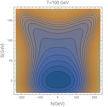
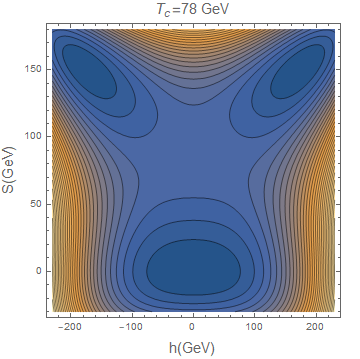
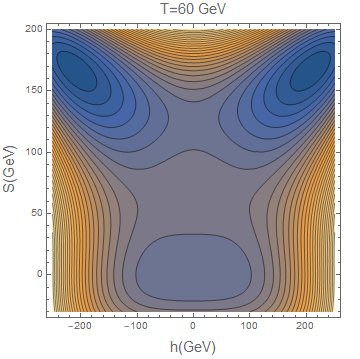
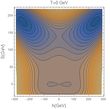
Figure 1: This is the phase transition process of $BM1$ (given in Table 1).

Depending on the vacuum structure at the zero temperature, there are two different phase transitions types, which are one-step PT $(0,0)\to(h,s)$ and two-step PT $(0,0)\to(h,0)/(0,s)\to(h,s)$, see Appendix. A for details. In this study, we focus on the one-step phase transition type. When the temperature of the Universe drops to the critical temperature, one have two potential degenerate at the vacua $O:(0,0)$ and $B:(h,s)$ occurring with a potential barrier structure. Where, one have

$$V_{T}(0,0,T_{C})=V_{T}(h_{B},s_{B},T_{C})\;,\frac{dV_{T}(h,s,T_{C})}{dh}|_{h=h_{B},s=s_{B}}=0\;,$$

$$\frac{dV_{T}(h,s,T_{C})}{ds}|_{h=h_{B},s=s_{B}}=0\;.$$ (21)

Through which, critical temperature and critical classical field value can be obtained. Here, we note that, to ensure two degenerate vacua occur the following constrains also should be satisfied (a positivitive determination of the finite temperature Hessian matrix): $M_{1}P_{1}-N_{1}^{2}>0,M_{1}>0$,where

$$\frac{d^{2}V_{T}(h,s,T_{C})}{dh^{2}}|_{h=h_{B},s=s_{B}}\equiv M_{1}\;,\frac{d^{2}V_{T}(h,s,T_{C})}{dhds}|_{h=h_{B},s=s_{B}}\equiv N_{1}\;,$$

$$\frac{d^{2}V_{T}(h,s,T_{C})}{ds^{2}}|_{h=h_{B},s=s_{B}}\equiv P_{1}\;.$$ (22)

We first select parameter points met $v_{c}/T_{c}>1$ at the critical temperature $T_{c}$ by using the above methodology, and then study if it is possible to have bubble nucleation, and if the phase transition can complete with CosmoTransitions Wainwright:2011kj . In Fig 1, we show that how the one-step phase transition process works ( $O(0,0)\to B(h,s)$). As the Universe cools down, a second minimum $B(h,s)$ develops, which indicate the break of the $\mathbb{Z}_{3}$ symmetry and EW symmetry, and the vacuum eventually becomes the present vacuum.

We choose $m_{\chi}$, $m_{2}$ ,$v_{s}$ and $\sin\theta$ as free parameters, and study the phase transition dynamics with these free parameter falls into the following ranges: $m_{\chi}\in[25,1000]\leavevmode\nobreak\ \rm{GeV}$, $m_{2}\in[200,1000]\leavevmode\nobreak\ \rm{GeV}$, $v_{s}\in[0,500]\leavevmode\nobreak\ \rm{GeV}$ and $|\sin\theta|\leq 0.37$ considering the mixing angle is constrained by the current measurements of the Higgs couplings at the LHC searches Ilnicka:2018def . For this study, the potential should be bounded from below with,

$$\lambda_{H}>0,\quad\lambda_{S}>0,\quad\lambda_{SH}+2\sqrt{\lambda_{H}\lambda_{S}}>0.$$ (23)

The unitarity constraints are,

$$|\lambda_{H}|\leqslant 4\pi,\quad|\lambda_{S}|\leqslant 4\pi,\quad|\lambda_{SH}|\leqslant 8\pi,$$ (24)

$$\lvert 3\lambda_{H}+2\lambda_{S}\pm\sqrt{9\lambda_{H}^{2}-12\lambda_{H}\lambda_{S}+4\lambda_{S}^{2}+2\lambda_{SH}^{2}}\rvert\leqslant 8\pi,$$ (25)

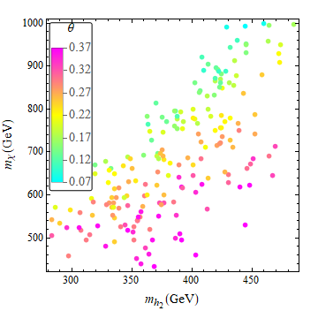
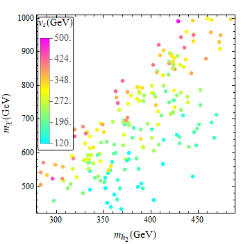
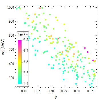
Figure 2: Left: the relation among $\theta$, $m_{\chi}$, and $m_{h_{2}}$ for EWPT points; Middle: the relation among $v_{s}$, $m_{\chi}$, and $m_{h_{2}}$ for EWPT points; Right: the phase transition strength $v_{n}/T_{n}$ as a function of $m_{\chi}$ and $\theta$.

In Fig. 2, we show the Electroweak phase transition points. The left (middle) panel indicates that a higher magnitude of $m_{\chi}$ and $m_{h_{2}}$ is accompanied with a small mixing angle $\theta$ (a higher magnitude of $v_{s}$) for the EWPT points. The right panel depicts that a stronger phase transition can be obtained with a large pseudo-scalar mass $m_{\chi}$ and a large mixing angle $\theta$.

III.2 BNPC and SFOEWPT

In this section, we estimate the strongly first-order phase transition condition through the estimation of the BNPC Patel:2011th . We first calculate the Electroweak sphaleron energy $E_{\rm sph}(T)$ at the phase transition temperature, and then check the relation between the phase transition strength $v(T)/T$ and the following quantity as suggested in Refs. Zhou:2020xqi ; Zhou:2019uzq ,

$$PT_{sph}\equiv\frac{E_{\rm sph}(T)}{T}-7\ln\frac{v(T)}{T}+\ln\frac{T}{100\rm{GeV}}\;.$$ (26)

With the quantity $PT_{sph}$ obtained above, we check if the BNPC can met as required by the successful baryon asymmetry generation within the Electroweak baryogengesis Patel:2011th ; Morrissey:2012db by the following condition Gan:2017mcv :

$$PT_{sph}>(35.9-42.8)\;.$$ (27)

The numerical range here mostly come from the uncertainty of the fluctuation determinant $\kappa=(10^{-4}-10^{-1})$ Dine:1991ck , which is estimated to be comparable with the uncertainty in the lattice simulation of the sphaleron rate at the Standard Model Electroweak cross-over DOnofrio:2014rug ; Gan:2017mcv .

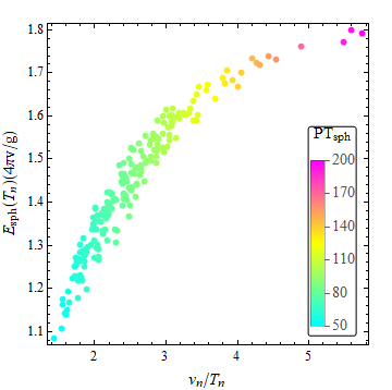
Figure 3: The $PT_{sph}$ as a function of the Electroweak sphaleron energy at nucleation temperature and the phase transition strength $v_{n}/T_{n}$.

In figure 3, it is clearly that all the phase transition points satisfy the BNPC, the sphaleron energy $E_{sph}(T_{n})$ and $PT_{sph}$ increase with the phase transition strength $v_{n}/T_{n}$ increases, and washout of the baryon asymmetry can be avoided. For uncertainty from Electroweak phase transition duration and bubble nucleation in the evaluation of BNPC, we refer to Ref. Patel:2011th .

IV Gravitational Waves

Since, we have the Electroweak symmetry breaking and $\mathbb{Z}_{3}$ breaking simultaneously, we expect two source of the gravitational radiation at the early Universe. In this section, we study the stochastic gravitational wave from the strongly first-order Electroweak phase transition and the domain wall decay at latter time.

IV.1 GW from EWPT

As a crucial parameter for the gravitational wave, $\alpha$ (which is the energy budget of SFOEWPT normalized by the radiative energy) is defined as

$$\alpha=\frac{\Delta\rho}{\rho_{R}}\;.$$ (28)

Here, $\rho_{R}=\pi^{2}g_{\star}T_{\star}^{4}/30$ is radiation energy of the bath or the plasma background, and $\Delta\rho$ is the latent heat from the phase transition to the energy density of the radiation bath or the plasma background. We take $T_{\star}\approx T_{n}$. There is another parameter $\beta$ which characterizes the inverse time duration of the SFOEWPT. Then the GW spectrum peak frequency is defined as

$$\frac{\beta}{H_{n}}=T\frac{d(S_{3}(T)/T)}{dT}|_{T=T_{n}}\;.$$ (29)

Both the two parameter can be obtained after the solution of the bounce. The action of the bounce configuration of the field that connects the Electroweak broken vacuum (true vacuum, $\mathbb{Z}_{3}$ broken) and the Electroweak preserving vacuum (false vacuum, $\mathbb{Z}_{3}$ preserving),

$$S_{3}(T)=\int 4\pi r^{2}dr\bigg{[}\frac{1}{2}\big{(}\frac{d\phi_{b}}{dr}\big{)}^{2}+V(\phi_{b},T)\bigg{]}\;,$$ (30)

through solving the equation of motion for $\phi_{b}$ (it is subspace of $h$ and $s$ for this study), with the boundary conditions of

$$\lim_{r\rightarrow\infty}\phi_{b}=0\;,\quad\quad\frac{d\phi_{b}}{dr}|_{r=0}=0\;.$$ (31)

The phase transition completes at the nucleation temperature when the thermal tunneling probability for bubble nucleation per horizon volume and per horizon time is of order unity Affleck:1980ac ; Linde:1981zj ; Linde:1980tt :

$$\Gamma\approx A(T)e^{-S_{3}/T}\sim 1\;.$$ (32)

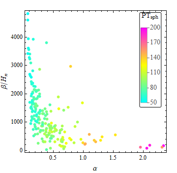
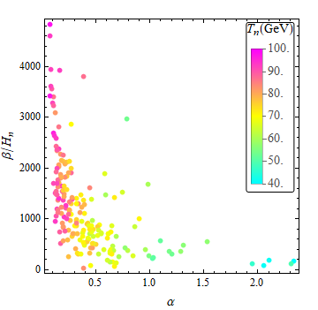
Figure 4: Left: We plot the relations between $\alpha$ and $\beta/H_{n}$ with the $PT_{sph}$ as color-code; Right: we show GW parameters $\beta/H_{n}$ and $\alpha$ relation, with nucleation temperature $T_{n}$ as color-code.

Before going to the study of gravitational wave, we first present the relation between the quantity of $PT_{sph}$ and the two crucial parameters for gravitational wave ($\alpha,\beta/H_{n}$) in the left panel of the Fig. 4. With a smaller $\beta/H_{n}$ (i.e., a long phase transition duration time) and a larger $\alpha$ (a larger phase transition strength), we obtain a larger $PT_{sph}$. Therefore, the BNPC can be satisfied much better. In the right panel of the Fig. 4, we present the relation among the nucleation temperature $T_{n}$ and the gravitational wave ($\alpha,\beta/H_{n}$). Which depicts that a large $\alpha$ along with a small $\beta/H_{n}$ can be obtained for a small $T_{n}$, one can expect a detectable gravitational wave there Alves:2018jsw . Indeed, the two plots also tell that a lower bubble nucleation temperature $T_{n}$ leads to a larger $PT_{sph}$.

The GWs from the EWPT mainly come from sound waves and MHD turbulence, with the total energy being given by Caprini:2015zlo

$$\Omega_{\rm GW}h^{2}(f)\approx\Omega h^{2}_{\rm sw}(f)+\Omega h^{2}_{\rm turb}(f)\;.$$ (33)

Here, we consider detonation bubble and take the bubble wall velocity $v_{b}$ and the efficiency factor $\kappa$ are functions of $\alpha$ Steinhardt:1981ct ,

$$v_{b}=\frac{1/\sqrt{3}+\sqrt{\alpha^{2}+2\alpha/3}}{1+\alpha},\quad\kappa=\frac{\alpha_{\infty}}{\alpha}\left(\frac{\alpha_{\infty}}{0.73+0.083\sqrt{\alpha_{\infty}}+\alpha_{\infty}}\right).$$ (34)

The peak frequency of the sound wave locates atHindmarsh:2013xza ; Hindmarsh:2015qta

$$f_{\rm sw}=1.9\times 10^{-5}\frac{\beta}{H}\frac{1}{v_{b}}\frac{T_{*}}{100}\left({\frac{g_{*}}{100}}\right)^{\frac{1}{6}}{\rm Hz}\;,$$ (35)

with the following energy density being given by

$$\Omega h^{2}_{\rm sw}(f)=2.65\times 10^{-6}\left(\frac{\beta}{H}\right)^{-1}\left(\frac{\kappa\alpha}{1+\alpha}\right)^{2}\left(\frac{g_{*}}{100}\right)^{-\frac{1}{3}}v_{b}\left(\frac{f}{f_{\rm sw}}\right)^{3}\left(\frac{7}{4+3\left(f/f_{\rm sw}\right)^{2}}\right)^{7/2}.$$ (36)

Here, the $\kappa$ describes the fraction of the latent heat transferred into the kinetic energy of plasma, we obtain the value by consider the the hydrodynamic analysis Espinosa:2010hh . The MHD turbulence in the plasma is the second important source of GW signals from phase transition, the peak frequency locates at Caprini:2009yp

$$f_{\rm turb}=2.7\times 10^{-5}\frac{\beta}{H}\frac{1}{v_{b}}\frac{T_{*}}{100}\left({\frac{g_{*}}{100}}\right)^{\frac{1}{6}}{\rm Hz}\;,$$ (37)

and the energy density is

$$\Omega h^{2}_{\rm turb}(f)=3.35\times 10^{-4}\left(\frac{\beta}{H}\right)^{-1}\left(\frac{\epsilon\kappa\alpha}{1+\alpha}\right)^{\frac{3}{2}}\left(\frac{g_{*}}{100}\right)^{-\frac{1}{3}}v_{b}\frac{\left(f/f_{\rm turb}\right)^{3}\left(1+f/f_{\rm turb}\right)^{-\frac{11}{3}}}{\left[1+8\pi fa_{0}/(a_{*}H_{*})\right]}\;,$$ (38)

where the efficiency factor $\epsilon\approx 0.05$, and the precent Hubble parameter

$$h_{\ast}=\bigl{(}1.65\times 10^{-5}Hz\bigr{)}\left(\frac{T_{*}}{100\rm{GeV}}\right)\left(\frac{g_{\ast}}{100}\right)^{1/6}\;.$$ (39)

IV.2 GW from domain wall decay

To get domain wall solution formed after the phase transition Vilenkin:2000jqa , we first introduce the phase of the singlet as $S=v_{s}e^{i\phi}$, and get the potential of $\phi$ as:

$$V=\frac{\mu_{H}^{2}}{2}v^{2}+\frac{\lambda_{H}}{4}v^{4}+\frac{\mu_{S}^{2}}{2}v_{s}^{2}+\frac{\lambda_{S}}{4}v_{s}^{4}+\frac{\lambda_{SH}}{4}v_{s}^{2}v^{2}+\frac{\mu_{3}}{2\sqrt{2}}v_{s}^{3}\cos(3\phi).$$ (40)

With $\eta^{2}=v_{s}^{2}/2$, the kinetic term of $\phi$ can be obtained as,

$$\mathcal{L}_{\text{kinetic }}(\phi)=\eta^{2}\left(\partial_{\mu}\phi\right)\left(\partial^{\mu}\phi\right)\;.$$ (41)

The field equation,

$$\partial_{\mu}\frac{\partial\mathcal{L}_{\text{kinetic }}}{\partial_{\mu}(\partial\phi)}+\frac{\partial V}{\partial\phi}=0\;,$$ (42)

yields

$$\frac{\mathrm{d}^{2}\phi}{\mathrm{d}z^{2}}-\frac{1}{3B^{2}}\sin(3\phi)=0\;,$$ (43)

with

$$\frac{1}{B^{2}}=-\frac{9}{4}\mu_{3}v_{s}^{2}\;,\phi=\frac{4}{3}\arctan(e^{\frac{z}{B}})\;.$$ (44)

From which, we can consider a planar domain wall orthogonal to the z-axis Hattori:2015xla , i.e., $\phi(z)$. The domain wall tension is estimated as,

$$\sigma=\int dz\rho_{\text{wall }}(z)=\int\bigg{(}\bigg{|}\frac{dS}{dz}\bigg{|}^{2}+V\bigg{(}\frac{S(z)}{\sqrt{2}},\frac{v}{\sqrt{2}}\bigg{)}-V\bigg{(}\frac{v_{s}}{\sqrt{2}},\frac{v}{\sqrt{2}}\bigg{)}\bigg{)}dz\;.$$ (45)

The same as the previous study of GWs at EWPT, we assume the gravitational radiation produced in the radiation dominated era. After the formation of the domain wall after the EWPT, one have the domain wall decay. With the peak frequency is given by the Hubble parameter at the decay time Hiramatsu:2013qaa :

$$f^{dw}\left(t_{0}\right)_{\mathrm{peak}}=\frac{a\left(t_{\mathrm{dec}}\right)}{a\left(t_{0}\right)}H\left(t_{\mathrm{dec}}\right)\simeq 3.99\times 10^{-9}\mathrm{Hz}\mathcal{A}^{-1/2}\left(\frac{1\mathrm{TeV}^{3}}{\sigma_{\mathrm{wall}}}\right)^{1/2}\left(\frac{\Delta V}{1\mathrm{MeV}^{4}}\right)^{1/2}\;,$$ (46)

and peak amplitude of the gravitational waves at the present time $t_{0}$ is estimated as Hiramatsu:2013qaa ; Kadota:2015dza

$$\Omega^{dw}_{\mathrm{GW}}h^{2}\left(t_{0}\right)_{\mathrm{peak}}\simeq 5.20\times 10^{-20}\times\tilde{\epsilon}_{\mathrm{gw}}\mathcal{A}^{4}\left(\frac{10.75}{g_{*}}\right)^{1/3}\left(\frac{\sigma_{\mathrm{wall}}}{1\mathrm{TeV}^{3}}\right)^{4}\left(\frac{1\mathrm{MeV}^{4}}{\Delta V}\right)^{2}.$$ (47)

Requiring the domain wall decay before they overclose Universe yields,

$$\sigma_{wall}<2.93\times 10^{4}\mathrm{TeV}^{3}\mathcal{A}^{-1}(\frac{0.1sec}{t_{dec}})\;.$$ (48)

The bias term $\Delta V$ in Eq. (46,47) here is introduced to explicitly break the $\mathbb{Z}_{3}$ symmetry, which determines the decay time of the domain wall,

$$t_{dec}\approx\mathcal{A}\sigma_{wall}/(\Delta V)\;.$$ (49)

Requiring the domain wall decay before the BBN with $t_{dec}\leq 0.01sec$ Kawasaki:2004yh ; Kawasaki:2004qu , one has a lower limit on the magnitude of the bias term:

$$\Delta V\gtrsim 6.6\times 10^{-2}\mathrm{MeV}^{4}\mathcal{A}\left(\frac{\sigma_{wall}}{1\mathrm{TeV}^{3}}\right)\;.$$ (50)

We note that the magnitude of the bias term should be much less than that of the potential around the core of domain walls ($\Delta V\ll V$ ) such that the discrete $\mathbb{Z}_{3}$-symmetry holds approximately and not affect the phase transition dynamics. In this study, we take the area parameter $\mathcal{A}=1.2$ for $\mathbb{Z}_{3}$ symmetry as in Ref Kadota:2015dza , the efficiency parameter $\tilde{\epsilon}_{\mathrm{gw}}=0.7$ Hiramatsu:2013qaa , and the degree of freedom at the domain wall decay time $g_{*}=10.75$  Kadota:2015dza . The whole spectrum of the gravitational wave can be obtained after considering the slope of spectrum $\Omega_{GW}^{dw}h^{2}\propto f^{3}$ when $f\textless f_{peak}$, and $\Omega^{dw}_{GW}h^{2}\propto f^{-1}$ when $f\geqslant f_{peak}$ as estimated in Ref Hiramatsu:2013qaa .

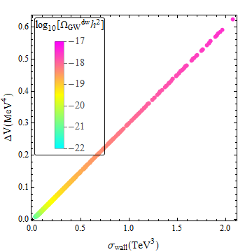
Figure 5: We show the relation between the surface mass density $\sigma_{wall}$ and the bias term $\Delta V$, with the $\Omega^{dw}_{GW}h^{2}$ as the color-code.

Eq. 46 and Eq. 47 indicate that $f^{dw}_{peak}$ is proportional to $\left(\frac{\Delta V}{\sigma_{\mathrm{wall}}}\right)^{1/2}$ and $\Omega_{GW}^{dw}h^{2}$ is proportional to $\sigma_{\mathrm{wall}}^{4}$. In order to evaluate the detectability of the GW from the domain from the SFOEWPT, we fix $f^{dw}_{peak}\approx 2\times 10^{-9}Hz$ at the sensitivity frequency of PPTA Hobbs:2013aka to get $\Delta V$ from the the Eq. 46 with $\sigma_{wall}$ calculated using the SFOEWPT allowed points. As we can see in Fig. 5, with increase of $\sigma_{wall}$ and $\Delta V$, $\Omega_{GW}^{dw}h^{2}$ can reach to $3.56\times 10^{-18}$, which is far beyond the sensitivity of the current PTA and the future SKA. Ref. Saikawa:2017hiv shows that a higher magnitude of the gravitational wave spectrum from the domain wall decay requires a large surface mass density of domain walls, which cannot be realized in the SFOEWPT parameter spaces in this model.

IV.3 GW from EWPT with domain wall decay

	$m_{\chi}$ (GeV)	$m_{h_{2}}$ (GeV)	$v_{s}$ (GeV)	$\theta$	$T_{n}$ (GeV)	$\beta/H_{n}$	$\alpha$
$BM_{1}$	625.08	361.31	184.10	0.30	50.16	219.62	1.02
$BM_{2}$	814.81	370.24	243.05	0.13	69.46	152.41	0.66

Table 1: Benchmarks in the Fig. 6.

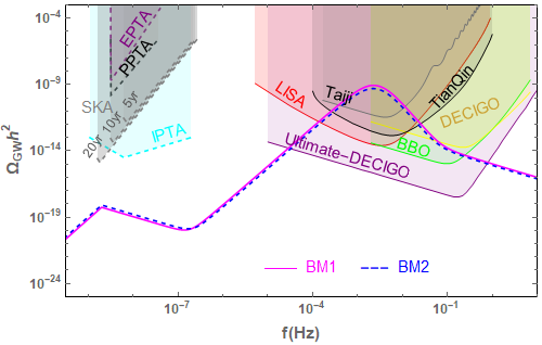
Figure 6: Gravitational wave signals from the strong first order electroweak phase transition with domain wall formation and decay.

We present the gravitational radiation from SFOEWPT and domain wall decay in Fig. 6 after sum the two contributions. The strength of GW from SFOEWPT is dominant in the higher frequency, and GW strength from the domain wall decay controls the GW spectrum of the low frequency. The gravitational wave signal spectrum with the second higher peak locates around $f_{peak}\sim 10^{-3}-10^{-2}$ Hz can be probed by the projected space-based interferometers, such as: LISA Klein:2015hvg , BBO Corbin:2005ny , DECIGO (Ultimate-DECIGO) Kudoh:2005as ; Musha:2017usi , TianQin  Luo:2015ght and Taiji Gong:2014mca programs. While, the first lower peak from domain wall decay is beyond the sensitivity of EPTA, PPTA, IPTA, and SKA.

V Conclusion and discussion

With the complex singlet scalar preserving $\mathbb{Z}_{3}$ symmetry, we study the possibility to achieve a one-step strongly first order Electroweak phase transition after considering the baryon number preservation criterion. After that, we studied the gravitational wave prediction from the strongly first-order Electroweak phase transition with domain wall decay, a two-peak shape is found as expected. The peak of the predicted gravitational wave signal from the domain wall decay locates around $f_{peak}^{dw}\sim\mathcal{O}(10^{-9})Hz$ with the amplitude of the spectrum cannot be probed by the current sensitivity region of EPTA, PPTA, and IPTA. The peak of the predicted GW spectrum from the phase transition locates at around $f_{peak}^{pt}\sim\mathcal{O}(10^{-3}-10^{-2})Hz$, with the amplitude within the capability of the projected space-base interferometers, such as: LISA, BBO, DECIGO, UDECIGO, TianQin and Taiji.

VI Acknowledgements

This work is supported by the National Natural Science Foundation of China under grant No.11605016 and No.11647307, and the Fundamental Research Fund for the Central Universities of China (No. 2019CDXYWL0029). We are grateful to Tanmay Vachaspati, Alexander Vilenkin, Ken’ichi Saikawa, Salah Nasri, and Michael J. Ramsey-Musolf for helpful communications and discussions.

Appendix A Vacuum structures and phase transition types

As shown in Fig. 7, there are totally four possible vacuums locate at $(0,0)$,$(h,0)$,$(0,s)$, and $(h,s)$.

$$O\leavevmode\nobreak\ point\leavevmode\nobreak\ :\leavevmode\nobreak\ h\to 0,S\to 0\;,$$

$$A\leavevmode\nobreak\ point\leavevmode\nobreak\ :\leavevmode\nobreak\ h\to 0,S\to\frac{9\mu_{3}^{2}-16\lambda_{S}\mu_{S}^{2}-3\sqrt{9\mu_{3}^{4}-32\lambda_{S}\mu_{3}^{2}\mu_{S}^{2}}}{16\lambda_{S}^{2}}\;,$$

$$B\leavevmode\nobreak\ point\leavevmode\nobreak\ :\leavevmode\nobreak\ h\to h_{B},S\to S_{B}\;,$$

$$C\leavevmode\nobreak\ point\leavevmode\nobreak\ :\leavevmode\nobreak\ h\to\sqrt{\frac{-\mu_{H}^{2}}{\lambda_{H}}},S\to 0\;.$$

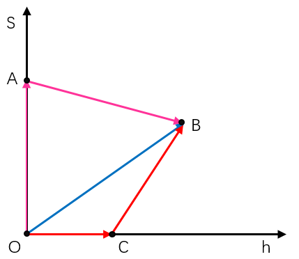
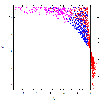
Figure 7: Left: The tree level potential vacuum structure of $\mathbb{Z}_{3}$ model. Right: We show the three types PT points distribution in the $\theta-\lambda_{SH}$ plane.

Therefore, three types phase transition process could happen: One of them is one-step PT ($O\to B$)(Blue), and two-step PT ($O\to A(C)\to B$) (Magenta(Red)). The one-step PT points gather around the $\theta>0$ region. For parameter space with a negative $\theta$, the two-step $O\to C\to B$ could take place. Meanwhile, the two-step PT ($O\to A\to B$) occurs with $\theta\geq 0.35$ that is not favored by the current LHC measurements.

Appendix B Electroweak sphaleron

To compute $E_{sph}(T)$, we obtain the sphaleron solutions following a method suggested in Refs Manton:1983nd ; Klinkhamer:1984di . Since $U(1)_{Y}$ contributions are sufficiently small Klinkhamer:1990fi ; James:1992re , we employ the spherically symmetric ansatz. Specifically, we consider the configuration of gauge, Higgs and singlet scalar fields are expressed as:

$$A_{i}(\mu,r,\theta,\phi) =-\frac{i}{g}f(r)\partial_{i}U(\mu,\theta,\phi)U^{-1}(\mu,\theta,\phi),$$ (51)

$$H(\mu,r,\theta,\phi) =\frac{v[T]}{\sqrt{2}}\left[(1-h(r))\left(\begin{array}[]{c}0\\ e^{-i\mu}\cos\mu\end{array}\right)+h(r)U(\mu,\theta,\phi)\left(\begin{array}[]{c}0\\ 1\end{array}\right)\right],$$ (56)

$$S(\mu,r,\theta,\phi) =\frac{v_{s}(T)}{\sqrt{2}}s(r).$$ (57)

where $A_{i}$ are SU(2) gauge fields, $A_{i}=\frac{1}{2}A_{i}^{a}\tau^{a}$, and $U(\mu,\theta,\phi)$ is defined as

$$U(\mu,\theta,\phi)=\left(\begin{array}[]{cc}e^{i\mu}(\cos\mu-i\sin\mu\cos\theta)&e^{i\phi}\sin\mu\sin\theta\\ -e^{-i\phi}\sin\mu\sin\theta&e^{-i\mu}(\cos\mu+i\sin\mu\cos\theta)\end{array}\right),$$ (60)

The sphaleron energy in the finite temperature can be written as:

$$E_{\rm sph}(T)=\frac{4\pi\Omega[T]}{g}\int_{0}^{\infty}\!d\xi\,\Bigl{[}4\biggl{(}\frac{df}{d\xi}\biggr{)}^{2}s_{\mu}^{2}+\frac{8}{\xi^{2}}f^{2}\bigl{(}1-f\bigr{)}^{2}s_{\mu}^{4}+\frac{\xi^{2}v[T]^{2}}{2\Omega[T]^{2}}\biggl{(}\frac{dh}{d\xi}\biggr{)}^{2}s_{\mu}^{2}$$

$$\qquad+\frac{\xi^{2}v_{s}[T]^{2}}{2\Omega[T]^{2}}\biggl{(}\frac{ds}{d\xi}\biggr{)}^{2}+s_{\mu}^{2}\frac{v[T]^{2}}{\Omega[T]^{2}}(\bigl{(}1-f\bigr{)}^{2}h^{2}-2fh(1-f)(1-h)c_{\mu}^{2}+f^{2}(1-h)^{2}c_{\mu}^{2})$$

$$\qquad+\frac{\xi^{2}}{g^{2}\Omega[T]^{4}}V_{eff}[\mu,h,s,T]\Bigr{]}$$ (61)

with $\mu\in[0,\pi]$. The configuration at $\mu=\pi/2$ corresponds to the sphaleron, where $\xi=g\Omega[T]r$, and the $V_{eff}[\mu,h,s,T]=V_{potential}[\mu,h,s,T]-|\Delta[T]|$, and $\Delta[T]$ is the cosmological constant energy density. And the $\Delta[T]$ can be regarded as the minimal value of the potential at temperature $T$. For example, in the $\mathbb{Z}_{3}$ after the temperature cooling at $T=0$ GeV, the constant energy density $\Delta[T]=V_{potential}[\mu,v,v_{s},T]$. That is to say, $Min[V_{eff}[\mu,h,s,T]]=0\leavevmode\nobreak\ \rm{GeV}^{4}$. The parameter $\Omega[T]$ can take any nonvanishing value of mass dimension one (for example $v[T]$, $v_{S}[T]$ or $\sqrt{v[T]^{2}+v_{S}[T]^{2}}$);

From Eq. (B), the equations of motion are found to be

$$\frac{d^{2}f}{d\xi^{2}}=\frac{2}{\xi^{2}}f(1-f)(1-2f)s_{\mu}^{2}+\frac{1}{4}(h^{2}(f-1)-h(1-h)(1-2f)c_{\mu}^{2}+f(1-h)^{2}c_{\mu}^{2})\;,$$

$$\frac{d}{d\xi}\left(\xi^{2}\frac{dh}{d\xi}\right)=2h(1-f)^{2}-2f(1-f)(1-2h)c_{\mu}^{2}-2f^{2}(1-h)c_{\mu}^{2}+\frac{\xi^{2}}{g^{2}}\frac{1}{v[T]^{2}\Omega[T]^{2}}\frac{\partial V_{\rm eff}}{\partial h}\;,$$

$$\frac{d}{d\xi}\left(\xi^{2}\frac{ds}{d\xi}\right)=\frac{\xi^{2}}{g^{2}}\frac{1}{v_{S}[T]^{2}\Omega[T]^{2}}\frac{\partial V_{\rm eff}}{\partial s}\;.$$ (62)

The sphaleron solutions could be obtained with the boundary condition,

$$\lim_{\xi\to 0}f(\xi)=0,\quad\lim_{\xi\to 0}h(\xi)=0,\quad\lim_{\xi\to 0}s^{\prime}(\xi)=0,$$ (63)

$$\lim_{\xi\to\infty}f(\xi)=1,\quad\lim_{\xi\to\infty}h(\xi)=1,\quad\lim_{\xi\to\infty}s(\xi)=1.$$ (64)

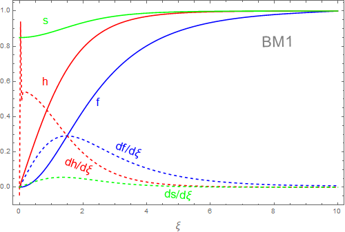
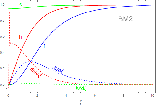
Figure 8: Numerically solved Sphaleron($\mu=\pi/2$) profiles of f, h, s and their derivatives as a function of the dimensionless quantity $\xi$ for the two benchmarks in Table 1.

In Fig. 8, we demonstrate the profile of the Higgs field, $SU(2)$ gauge field, singlet scalar field, and their derivatives behavior, respectively. In Fig. 9, we illustrate that the sphaleron energy $E_{sph}(T)$ and VEVs of $h(v_{h})$ and $s(v_{s})$ decrease as the temperature drops for the two benchmark points in Table 1. The sphaleron energy $E_{sph}(T)$ is highly sensitive to the VEV of $h$, as indicated in Ref. Patel:2011th .

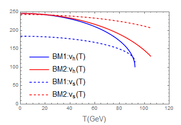
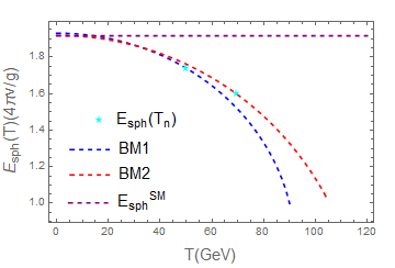
Figure 9: Left: Finite temperature VEVs of h(blue) and s(red) versus $T$ for SFOEWPT points. Right: EW sphaleron energy as a function of temperature.

References

- (1) B. P. Abbott et al. [LIGO Scientific and Virgo Collaborations], Phys. Rev. Lett. 116, no. 6, 061102 (2016) doi:10.1103/PhysRevLett.116.061102 [arXiv:1602.03837 [gr-qc]].
- (2) P. Amaro-Seoane et al. [LISA Collaboration], arXiv:1702.00786 [astro-ph.IM].
- (3) D. E. Morrissey and M. J. Ramsey-Musolf, New J. Phys. 14, 125003 (2012) doi:10.1088/1367-2630/14/12/125003.
- (4) C. Caprini et al., arXiv:1910.13125 [astro-ph.CO].
- (5) M. D’Onofrio, K. Rummukainen and A. Tranberg, Phys. Rev. Lett. 113, no. 14, 141602 (2014) doi:10.1103/PhysRevLett.113.141602 [arXiv:1404.3565 [hep-ph]].
- (6) A. Mazumdar and G. White, Rept. Prog. Phys. 82, no. 7, 076901 (2019) doi:10.1088/1361-6633/ab1f55 [arXiv:1811.01948 [hep-ph]].
- (7) N. Arkani-Hamed, T. Han, M. Mangano and L. T. Wang, Phys. Rept. 652, 1 (2016) doi:10.1016/j.physrep.2016.07.004 [arXiv:1511.06495 [hep-ph]].
- (8) N. Chen, T. Li, Y. Wu and L. Bian, arXiv:1911.05579 [hep-ph].
- (9) A. Alves, D. Gon?alves, T. Ghosh, H. K. Guo and K. Sinha, arXiv:1909.05268 [hep-ph].
- (10) K. Hashino, R. Jinno, M. Kakizaki, S. Kanemura, T. Takahashi and M. Takimoto, Phys. Rev. D 99, no. 7, 075011 (2019) doi:10.1103/PhysRevD.99.075011 [arXiv:1809.04994 [hep-ph]].
- (11) K. Hashino, M. Kakizaki, S. Kanemura and T. Matsui, Phys. Rev. D 94, no. 1, 015005 (2016) doi:10.1103/PhysRevD.94.015005 [arXiv:1604.02069 [hep-ph]].
- (12) L. Bian, H. K. Guo, Y. Wu and R. Zhou, arXiv:1906.11664 [hep-ph].
- (13) A. Alves, T. Ghosh, H. K. Guo, K. Sinha and D. Vagie, JHEP 1904, 052 (2019) doi:10.1007/JHEP04(2019)052 [arXiv:1812.09333 [hep-ph]].
- (14) T. W. B. Kibble, J. Phys. A 9, 1387 (1976). doi:10.1088/0305-4470/9/8/029
- (15) A. Vilenkin, Phys. Rev. D 23, 852 (1981). doi:10.1103/PhysRevD.23.852
- (16) G. B. Gelmini, M. Gleiser and E. W. Kolb, Phys. Rev. D 39, 1558 (1989). doi:10.1103/PhysRevD.39.1558
- (17) S. E. Larsson, S. Sarkar and P. L. White, Phys. Rev. D 55, 5129 (1997) doi:10.1103/PhysRevD.55.5129 [hep-ph/9608319].
- (18) Z. Kang, P. Ko and T. Matsui, JHEP 1802, 115 (2018) doi:10.1007/JHEP02(2018)115 [arXiv:1706.09721 [hep-ph]].
- (19) K. Kannike, K. Loos and M. Raidal, arXiv:1907.13136 [hep-ph].
- (20) C. W. Chiang and B. Q. Lu, arXiv:1912.12634 [hep-ph].
- (21) G. Desvignes et al., Mon. Not. Roy. Astron. Soc. 458, no. 3, 3341 (2016) doi:10.1093/mnras/stw483 [arXiv:1602.08511 [astro-ph.HE]].
- (22) G. Hobbs, Class. Quant. Grav. 30, 224007 (2013) doi:10.1088/0264-9381/30/22/224007 [arXiv:1307.2629 [astro-ph.IM]].
- (23) J. P. W. Verbiest et al., Mon. Not. Roy. Astron. Soc. 458, no. 2, 1267 (2016) doi:10.1093/mnras/stw347 [arXiv:1602.03640 [astro-ph.IM]].
- (24) A. Ilnicka, T. Robens and T. Stefaniak, Mod. Phys. Lett. A 33, no. 10n11, 1830007 (2018) doi:10.1142/S0217732318300070 [arXiv:1803.03594 [hep-ph]].
- (25) R. Zhou, W. Cheng, X. Deng, L. Bian and Y. Wu, JHEP 1901, 216 (2019) doi:10.1007/JHEP01(2019)216 [arXiv:1812.06217 [hep-ph]].
- (26) L. Bian, Y. Wu and K. P. Xie, JHEP 1912, 028 (2019) doi:10.1007/JHEP12(2019)028 [arXiv:1909.02014 [hep-ph]].
- (27) L. Bian and X. Liu, Phys. Rev. D 99, no. 5, 055003 (2019) doi:10.1103/PhysRevD.99.055003 [arXiv:1811.03279 [hep-ph]].
- (28) L. Bian and Y. L. Tang, JHEP 1812, 006 (2018) doi:10.1007/JHEP12(2018)006 [arXiv:1810.03172 [hep-ph]].
- (29) W. Chao, H. K. Guo and J. Shu, JCAP 1709, 009 (2017) doi:10.1088/1475-7516/2017/09/009 [arXiv:1702.02698 [hep-ph]].
- (30) C. L. Wainwright, Comput. Phys. Commun. 183, 2006 (2012) doi:10.1016/j.cpc.2012.04.004 [arXiv:1109.4189 [hep-ph]].
- (31) H. H. Patel and M. J. Ramsey-Musolf, JHEP 1107, 029 (2011) doi:10.1007/JHEP07(2011)029 [arXiv:1101.4665 [hep-ph]].
- (32) R. Zhou and L. Bian, arXiv:2001.01237 [hep-ph].
- (33) R. Zhou, L. Bian and H. K. Guo, arXiv:1910.00234 [hep-ph].
- (34) X. Gan, A. J. Long and L. T. Wang, Phys. Rev. D 96, no. 11, 115018 (2017) doi:10.1103/PhysRevD.96.115018 [arXiv:1708.03061 [hep-ph]].
- (35) M. Dine, P. Huet and R. L. Singleton, Jr., Nucl. Phys. B 375, 625 (1992). doi:10.1016/0550-3213(92)90113-P
- (36) I. Affleck, Phys. Rev. Lett. 46, 388 (1981). doi:10.1103/PhysRevLett.46.388.
- (37) A. D. Linde, Nucl. Phys. B 216, 421 (1983) Erratum: [Nucl. Phys. B 223, 544 (1983)]. doi:10.1016/0550-3213(83)90293-6, 10.1016/0550-3213(83)90072-X.
- (38) A. D. Linde, Phys. Lett. 100B, 37 (1981). doi:10.1016/0370-2693(81)90281-1.
- (39) C. Caprini et al., JCAP 1604, 001 (2016) doi:10.1088/1475-7516/2016/04/001
- (40) P. J. Steinhardt, Phys. Rev. D 25, 2074 (1982). doi:10.1103/PhysRevD.25.2074
- (41) M. Hindmarsh, S. J. Huber, K. Rummukainen and D. J. Weir, Phys. Rev. Lett. 112, 041301 (2014) doi:10.1103/PhysRevLett.112.041301 [arXiv:1304.2433 [hep-ph]].
- (42) M. Hindmarsh, S. J. Huber, K. Rummukainen and D. J. Weir, Phys. Rev. D 92, no. 12, 123009 (2015) doi:10.1103/PhysRevD.92.123009 [arXiv:1504.03291 [astro-ph.CO]].
- (43) J. R. Espinosa, T. Konstandin, J. M. No, and G. Servant, “Energy Budget of Cosmological First-order Phase Transitions,” JCAP 1006 (2010) 028, arXiv:1004.4187 [hep-ph].
- (44) C. Caprini, R. Durrer and G. Servant, JCAP 0912, 024 (2009) doi:10.1088/1475-7516/2009/12/024 [arXiv:0909.0622 [astro-ph.CO]].
- (45) A. Vilenkin and E. P. S. Shellard,
- (46) H. Hattori, T. Kobayashi, N. Omoto and O. Seto, Phys. Rev. D 92, no. 10, 103518 (2015) doi:10.1103/PhysRevD.92.103518 [arXiv:1510.03595 [hep-ph]].
- (47) T. Hiramatsu, M. Kawasaki and K. Saikawa, JCAP 1402, 031 (2014) doi:10.1088/1475-7516/2014/02/031 [arXiv:1309.5001 [astro-ph.CO]].
- (48) K. Kadota, M. Kawasaki and K. Saikawa, JCAP 1510, 041 (2015) doi:10.1088/1475-7516/2015/10/041 [arXiv:1503.06998 [hep-ph]].
- (49) M. Kawasaki, K. Kohri and T. Moroi, Phys. Lett. B 625, 7 (2005) doi:10.1016/j.physletb.2005.08.045 [astro-ph/0402490].
- (50) M. Kawasaki, K. Kohri and T. Moroi, Phys. Rev. D 71, 083502 (2005) doi:10.1103/PhysRevD.71.083502 [astro-ph/0408426].
- (51) K. Saikawa, Universe 3, no. 2, 40 (2017) doi:10.3390/universe3020040 [arXiv:1703.02576 [hep-ph]].
- (52) A. Klein et al., Phys. Rev. D 93, no. 2, 024003 (2016) doi:10.1103/PhysRevD.93.024003 [arXiv:1511.05581 [gr-qc]].
- (53) V. Corbin and N. J. Cornish, Class. Quant. Grav. 23, 2435 (2006) doi:10.1088/0264-9381/23/7/014 [gr-qc/0512039].
- (54) H. Kudoh, A. Taruya, T. Hiramatsu and Y. Himemoto, Phys. Rev. D 73, 064006 (2006) doi:10.1103/PhysRevD.73.064006 [gr-qc/0511145].
- (55) M. Musha [DECIGO Working group], Proc. SPIE Int. Soc. Opt. Eng. 10562, 105623T (2017). doi:10.1117/12.2296050
- (56) J. Luo et al. [TianQin Collaboration], Class. Quant. Grav. 33, no. 3, 035010 (2016) doi:10.1088/0264-9381/33/3/035010 [arXiv:1512.02076 [astro-ph.IM]].
- (57) X. Gong et al., J. Phys. Conf. Ser. 610, no. 1, 012011 (2015) doi:10.1088/1742-6596/610/1/012011 [arXiv:1410.7296 [gr-qc]].
- (58) N. S. Manton, Phys. Rev. D 28, 2019 (1983). doi:10.1103/PhysRevD.28.2019.
- (59) F. R. Klinkhamer and N. S. Manton, Phys. Rev. D 30, 2212 (1984). doi:10.1103/PhysRevD.30.2212.
- (60) M. E. R. James, Z. Phys. C 55, 515 (1992). doi:10.1007/BF01565115.
- (61) F. R. Klinkhamer and R. Laterveer, Z. Phys. C 53, 247 (1992). doi:10.1007/BF01597560.
- (62) A. Alves, T. Ghosh, H. K. Guo and K. Sinha, JHEP 1812, 070 (2018) doi:10.1007/JHEP12(2018)070 [arXiv:1808.08974 [hep-ph]].