Improvement of heavy-heavy and heavy-light currents with the Oktay-Kronfeld action

Abstract

The CKM matrix elements $|V_{cb}|$ and $|V_{ub}|$ can be obtained by combining data from the experiments with lattice QCD results for the semi-leptonic form factors for the $\bar{B}\to D^{\ast}\ell\bar{\nu}$ and $\bar{B}\to\pi\ell\bar{\nu}$ decays. It is highly desirable to use the Oktay-Kronfeld (OK) action for the form factor calculation on the lattice, since the OK action is designed to reduce the heavy quark discretization error down to the $\mathcal{O}(\lambda^{4})$ level in the power counting rules of the heavy quark effective theory (HQET). Here, we present a matching calculation to improve heavy-heavy and heavy-light currents up to the $\lambda^{3}$ order in HQET, the same level of improvement as the OK action. Our final results for the improved currents are being used in a lattice QCD calculation of the semi-leptonic form factors for the $\bar{B}\to D^{\ast}\ell\bar{\nu}$ and $\bar{B}\to D\ell\bar{\nu}$ decays.

I Introduction

The Cabibbo-Kobayashi-Maskawa (CKM) matrix contains four of the fundamental parameters of the Standard Model (SM) which describes flavor-changing phenomena and CP violation [1, 2].

The CKM matrix is a $3\times 3$ unitary matrix, and $|V_{cb}|$ is a CKM matrix element which describes flavor-changing weak interactions between bottom and charm quarks. $|V_{cb}|$ is an important quantity in particle physics. It constrains one side of the unitarity triangle through the ratio $|V_{ub}|/|V_{cb}|$. It gives the dominant uncertainty in the determination of the CP violation parameter $\varepsilon_{K}$ in the neutral kaon system, where there is currently tension between the SM and experiment [3].

There are two competing and independent methods to determine $|V_{cb}|$: one is to derive $|V_{cb}|$ from the exclusive decays ($\bar{B}\to D^{\ast}\ell\bar{\nu}$ and $\bar{B}\to D\ell\bar{\nu}$) and the other is to obtain $|V_{cb}|$ from the inclusive decays ($B\to X_{c}\ell\nu$). There exists currently $3\sigma\sim 4\sigma$ tension between the exclusive $|V_{cb}|$ and the inclusive $|V_{cb}|$ [4, 5], which makes the study of $|V_{cb}|$ even more interesting.

Another motivation to study the exclusive decays ($\bar{B}\to D^{\ast}\ell\bar{\nu}$ and $\bar{B}\to D\ell\bar{\nu}$) is the tension in $R(D^{(\ast)})$ between the SM theory and experiment [6]. An update from HFLAV [6] gave the combined tension in $R(D)$ and $R(D^{\ast})$ to be about $3.8\sigma$. A recent report from HFLAV [4] and BELLE [7] claimed that the tension is about $3\sigma$. Hence, more precise determination of the semi-leptonic form factors for the exclusive decays will be important to confirm or dismiss a potential new physics possibility.

When we determine $|V_{cb}|$ from the exclusive decays such as $\bar{B}\to D^{\ast}\ell\bar{\nu}$, there are two different sources of uncertainty: One comes from the theory, and the other comes from experiment. Basically the experiments determine $|V_{cb}|\cdot|\mathcal{F}(1)|$ and the theory determines the form factors $|\mathcal{F}(1)|$. The dominant uncertainty in the calculation of the semi-leptonic form factors $|\mathcal{F}(1)|$ comes from the heavy-quark discretization [8]. Hence, it is essential to reduce the heavy-quark discretization error as much as possible in order to achieve higher precision in $|\mathcal{F}(1)|$.

It is challenging to reduce the discretization errors for $b$ and $c$ quarks, since the heavy quark masses are comparable with or greater than the inverse of the lattice spacing $1/a$. The Symanzik improvement program [9] does not work for $am_{Q}\approx 1$. The Fermilab formalism [10] makes it possible to control the discretization errors of bottom and charm quarks on relatively coarse lattices. In the Fermilab formalism, the lattice artifacts for heavy quarks are bounded in the limit of $m_{Q}a\to\infty$, and they can be reduced systematically by tuning coefficients of the action. With a non-relativistic interpretation of the Wilson action, one can match the lattice theory to continuum QCD using the heavy-quark effective theory (HQET) for heavy-light systems [11, 12, 13] or non-relativistic QCD (NRQCD) for quarkonia [14, 15]. Here we can estimate the lattice artifacts due to neglecting the truncated higher order terms by using the power counting of HQET or NRQCD.

The Fermilab action includes the dimension five operators of the Wilson clover action and is improved up to the $\lambda^{1}$ order in HQET [10]. The Oktay-Kronfeld (OK) action is an extension of the Fermilab action and is improved up to the $\lambda^{3}$ order in HQET [16]. In order to calculate weak matrix elements while taking advantage of the full merits of the OK action, it is essential to improve also the flavor-changing currents up to the $\lambda^{3}$ order at the tree level. In this paper we explain additional operators needed to improve the currents up to the $\lambda^{3}$ order and a matching calculation to determine the coefficients for these operators. The resulting improved currents can be used to calculate the semi-leptonic form factors for the $\bar{B}\to D^{\ast}\ell\bar{\nu}$ and $\bar{B}\to D\ell\bar{\nu}$ decays [17, 18].

In Section II we briefly review the Fermilab formalism and show the explicit forms of the Fermilab and OK actions. In Section III we introduce an approach to current improvement and build up the improved current. In Section IV we explain the matching calculations and determine the improvement parameters, the coefficients for the improved current operators. In Section V we present an interpretation of the matching calculation based on HQET. The HQET interpretation clarifies the structure of the matching conditions and provides a cross-check. In Section VI we present the results for the improvement parameters and discuss their continuum and static limits. In Section VII we conclude. The appendices contain technical details on the matching calculations and comparison of the continuum limit with results from the Symanzik program.

Preliminary results for the improved currents were presented in [19].

II Lattice Actions for Heavy Quarks

The Fermilab method [10] is used to systematically improve lattice gauge theories with Wilson quarks [20] with masses comparable to the lattice cutoff, $am_{Q}\simeq 1$. Symanzik’s original local effective description of lattice gauge theory [9] assumes $am_{Q}\ll 1$, and so it does not apply to heavy quarks. Instead, HQET and NRQCD can be used as alternative effective field theories to describe the lattice artifacts of heavy quarks [21, 22, 23]. A dual expansion in $\lambda\sim\Lambda/(2m_{Q})\sim a\Lambda$ is used to construct the $\mathcal{O}(\lambda^{1})$ action of effective-continuum HQET. Using a generalized version of Symanzik’s effective field theory together with effective-continuum HQET and NRQCD, an improved version of the Fermilab action was developed in Ref. [16]. It is called the OK action, which includes improvement terms through $\mathcal{O}(\lambda^{3})$.

The Fermilab method begins with the observation that time-space axis-interchange symmetry need not be respected to tune the lattice action and currents to the renormalized trajectory [24]. For systems with heavy quarks, Ref. [10] introduced independent, mass-dependent couplings for the spatial and temporal parts of the clover term [25] and pointed out the sufficiency of including only spatial terms at higher order, without altering the Wilson time derivative. Constructing the transfer matrix and deriving the Hamiltonian, it is shown that the discretization errors remain bounded as $am_{Q}\to\infty$.

The analysis of the lattice Hamiltonian also led to introducing an improved quark field for flavor-changing currents [10]. Constructing flavor-changing currents with the improved quark fields, the coefficients of the improvement terms can be determined uniquely by matching two-quark matrix elements. In Refs. [22, 23], it was proven that for improvement through $\mathcal{O}(\lambda)$ in HQET it is sufficient to match the improved field at tree-level.

The equivalence of the lattice theory and HQET can be expressed by the relation

$$S_{\text{lat}}\doteq S_{\text{HQET}}=\int d^{4}x~{}\mathcal{L}_{\text{HQET}}\,,$$ (1)

where the symbol $\doteq$ means that, in the regime where both theories hold, all physical amplitudes with external states on shell are equal to each other, and

$$\mathcal{L}_{\text{HQET}}=\bar{h}^{+}\Big{(}D_{4}+m_{1}-\frac{\bm{D}^{2}}{2m_{2}}+\frac{z_{B}i\bm{\sigma\cdot B}}{2m_{B}}\Big{)}h^{+}+\cdots\,,$$ (2)

where $z_{B}$ is the matching coefficient for the chromomagnetic term, and $m_{1}$, $m_{2}$, and $m_{B}$ are the rest, kinetic, and chromomagnetic masses of the quark, respectively. Here, $h^{+}$ is a heavy-quark field which satisfies $\gamma_{4}h^{+}=h^{+}$. When we consider matching between the lattice theory and HQET, the rest mass $m_{1}$ makes no difference because it does not affect the energy splittings and the matrix elements [21]. The bare mass (or the hopping parameter) is determined by demanding that the kinetic mass $m_{2}$ be equal to the physical mass.

The explicit formula of the Fermilab action [10] is

$$S_{\text{Fermilab}}=S_{0}+S_{B}+S_{E},$$ (3)

where

$$S_{0}= a^{4}\sum_{x}\big{[}m_{0}\bar{\psi}(x)\psi(x)+\bar{\psi}(x)\gamma_{4}D_{\text{lat},4}\psi(x)$$

$$+\zeta\bar{\psi}(x)\bm{\gamma}\cdot\bm{D}_{\text{lat}}\psi(x)-\frac{1}{2}a\bar{\psi}(x)\Delta_{4}\psi(x)$$

$$-\frac{1}{2}r_{s}\zeta a\bar{\psi}(x)\Delta^{(3)}\psi(x)\big{]}\,,$$ (4)

where $m_{0}$ is a bare quark mass, the parameter $\zeta$ breaks axis-interchange symmetry if $\zeta\neq 1$, and $r_{s}$ is the Wilson parameter for the spatial directions. The lattice covariant derivative operators are

$$D_{\text{lat},\mu}\psi =(2a)^{-1}(T_{\mu}-T_{-\mu})\psi\,,$$ (5)

$$\Delta_{\mu}\psi =a^{-2}(T_{\mu}+T_{-\mu}-2)\psi\,,$$ (6)

$$\Delta^{(3)}\psi =\sum_{i=1}^{3}\Delta_{i}\psi\,,$$ (7)

where the covariant translation is defined by

$$T_{\pm\mu}\psi(x) =U_{\pm\mu}(x)\psi(x\pm a\hat{\mu})\,,$$ (8)

$$U_{\pm\mu}(x) =U(x,x\pm a\hat{\mu})\,,$$ (9)

where $\pm\mu$ represents the positive and negative directions along the $\mu$-axis, and $\hat{\mu}$ is a unit vector along the $\mu$-axis. The dimension five operators $S_{B}$ and $S_{E}$ are

$$S_{B} =-\frac{1}{2}c_{B}\zeta a^{5}\sum_{x}\bar{\psi}(x)i\bm{\Sigma}\cdot\bm{B}_{\text{lat}}\psi(x),$$ (10)

$$S_{E} =-\frac{1}{2}c_{E}\zeta a^{5}\sum_{x}\bar{\psi}(x)\bm{\alpha}\cdot\bm{E}_{\text{lat}}\psi(x)\,.$$ (11)

Here the chromomagnetic and the chromoelectric fields are

$$B_{\text{lat},i} =\frac{1}{2}\epsilon_{ijk}F^{\text{lat}}_{jk},\qquad E_{\text{lat},i}=F^{\text{lat}}_{4i},$$ (12)

with the clover field-strength tensor

$$F^{\text{lat}}_{\mu\nu}=\frac{1}{8a^{2}}\sum_{\bar{\mu}=\pm\mu,\atop\bar{\nu}=\pm\nu}\text{sign}(\bar{\mu})\text{sign}(\bar{\nu})T_{\bar{\mu}}T_{\bar{\nu}}T_{-\bar{\mu}}T_{-\bar{\nu}}-\text{h.c.}\,.$$ (13)

Here $\text{sign}(\bar{\mu})=\pm 1$ for $\bar{\mu}=\pm\mu$.

The OK action [16] includes counter-terms up to $\lambda^{3}$ order, incorporating all dimension six and some dimension seven bilinear operators. The OK action is

$$S_{\text{OK}}=S_{0}+S_{B}+S_{E}+S_{6}+S_{7}\,,$$ (14)

where $S_{6}$ ($S_{7}$) represents counter-terms of dimension six (seven). Explicitly,

$$S_{6}=a^{6}\sum_{x}\bar{\psi}(x)\Big{[}c_{1}\sum_{i}\gamma_{i}D_{\text{lat},i}\Delta_{\text{lat},i}+c_{2}\{\bm{\gamma}\cdot\bm{D}_{\text{lat}},\Delta^{(3)}\}$$

$$+c_{3}\{\bm{\gamma}\cdot\bm{D}_{\text{lat}},i\bm{\Sigma}\cdot\bm{B}_{\text{lat}}\}+c_{EE}\{\gamma_{4}D_{\text{lat},4},\bm{\alpha}\cdot\bm{E}_{\text{lat}}\}\Big{]}\psi(x)\,,$$ (15)

and

$$S_{7}=a^{7}\sum_{x}\bar{\psi}(x)\sum_{i}\Big{[}c_{4}\Delta_{i}^{2}+c_{5}\sum_{j\neq i}\{i\Sigma_{i}B_{\text{lat},i},\Delta_{j}\}\Big{]}\psi(x)\,.$$ (16)

The coefficients $\{c_{i}\}$ are determined by matching the dispersion relation, interaction with a background field, and Compton scattering amplitude at tree level.

Taking redundant operators into account, the operators in Eqs. (II) and (16) are a complete set for matching through $\mathcal{O}(\lambda^{3})$ at tree level. In general, at dimension six, there are contributions from not only bilinears, but also four-quark operators such as

$$[\bar{Q}\Gamma Q][\bar{Q}\Gamma Q]\,,$$ (17)

$$[\bar{Q}\Gamma Q]\displaystyle\sum_{f}[\bar{q}_{f}\Gamma q_{f}]\,,$$ (18)

where $Q$ represents heavy quarks, and $q_{f}$ represents light quarks with flavor $f$. In the heavy-light system, however, four-quark operators of the type in Eq. (17) contribute to physical matrix elements only through heavy-quark loops, and so contributions from these operators are suppressed by at least an additional factor of $\lambda^{2}$ [16]; such operators are omitted from the OK action. When [heavy quark]-[light quark] scattering is matched at tree level, one finds that the tree-level coupling of four-quark operators of the type in Eq. (18) is proportional to a redundant coupling of the pure-gauge action, and can be eliminated by adjusting this coupling [16]. Thus, the four-quark operators are neglected, and the OK action has only six new bilinear operators.

III Improvement terms for the lattice heavy quark currents

In the calculation of hadronic matrix elements for $\bar{B}\to D^{(*)}\ell\bar{\nu}$ decay, heavy-quark discretization errors come from both the hadronic states and the flavor-changing currents [21, 23]. Using the OK action for $b$ and $c$ quarks, we expect the hadronic states of the $B$ and $D^{(*)}$ mesons to be improved up to $\lambda^{3}$ order by the action itself. To take full advantage of the OK action for $b$ and $c$ quarks, we must improve the flavor-changing currents up to $\lambda^{3}$ order, the level of improvement of the OK action. Here we explain how to improve the currents up to $\lambda^{3}$ order using HQET.

The current improvement to first order in $\lambda$ was studied in [10, 21, 23]. If one neglects loop corrections, the current improvement can be done by introducing an improved quark field [10, 23].

$$V^{\text{lat}}_{\mu} =\bar{\Psi}_{Ic}\gamma_{\mu}\Psi_{Ib},$$ (19)

$$A^{\text{lat}}_{\mu} =\bar{\Psi}_{Ic}\gamma_{\mu}\gamma_{5}\Psi_{Ib},$$ (20)

where $\Psi_{If}$ is ($f=b,c$)

$$\Psi_{If}(x)\equiv e^{m_{1f}a/2}[1+ad_{1f}\bm{\gamma\cdot D_{\text{lat}}}]\psi_{f}(x)\,.$$ (21)

Here, the normalization factor $e^{m_{1f}a/2}$ is introduced to cancel out the field renormalization of the lattice quark fields : $m_{1f}a=\log(1+m_{0f}a)$ is the rest mass at tree level ($f=b,c$). The parameter $d_{1}$ is an improvement parameter to be determined by a matching condition. In [10, 23], it is shown that introducing the improved quark field Eq. (21) is enough for the current improvement at tree level.

Here we would like to extend the idea of the improved quark field to $\mathcal{O}(\lambda^{3})$. We need to find a complete set of operators up to dimension six. The continuum Foldy-Wouthuysen-Tani (FWT) transformation [26, 27] is a good starting point.

Let us review how to derive the HQET Lagrangian from the QCD Lagrangian. The fermionic part of the QCD Lagrangian in Euclidean space is

$$\mathcal{L}_{\text{Dirac}}=-\bar{Q}(\text{$\not\!\!D$}+m)Q\,,$$ (22)

where $Q$ is a heavy quark field with mass $m$. At tree level, the HQET Lagrangian can be derived by using a FWT transformation, which decouples quark and anti-quark. The FWT transformation up to $1/m^{4}$ order is

$$Q=\bigg{[}1-\frac{1}{2m}\bm{\gamma\cdot D}+\frac{1}{8m^{2}}(\bm{\gamma\cdot D})^{2}+\frac{1}{4m^{2}}\bm{\alpha}\cdot\bm{E}$$

$$-\frac{3(\bm{\gamma\cdot D})^{3}}{16m^{3}}-\frac{\bm{\gamma}\cdot\bm{D}\bm{\alpha}\cdot\bm{E}}{8m^{3}}-\frac{\{\gamma_{4}D_{4},\bm{\alpha}\cdot\bm{E}\}}{8m^{3}}$$

$$+\frac{11(\bm{\gamma\cdot D})^{4}}{128m^{4}}+\frac{3(\bm{\gamma\cdot D})^{3}\gamma_{4}D_{4}}{16m^{4}}$$

$$+\frac{(\bm{\gamma\cdot D})^{2}\gamma_{4}D_{4}(\bm{\gamma\cdot D})}{8m^{4}}+\frac{3(\bm{\gamma\cdot D})\gamma_{4}D_{4}(\bm{\gamma\cdot D})^{2}}{32m^{4}}$$

$$+\frac{5\gamma_{4}D_{4}(\bm{\gamma\cdot D})^{3}}{32m^{4}}+\frac{\bm{\gamma\cdot D}\{\gamma_{4}D_{4},\bm{\alpha\cdot E}\}}{16m^{4}}+\frac{(\bm{\alpha\cdot E})^{2}}{32m^{4}}$$

$$+\frac{1}{16m^{4}}\big{\{}\gamma_{4}D_{4},\{\gamma_{4}D_{4},\bm{\alpha\cdot E}\}\big{\}}\bigg{]}h+\mathcal{O}(1/m^{5})\,.$$ (23)

The corresponding HQET Lagrangian up to $1/m^{3}$ order is

$$\mathcal{L}_{HQ} =\bar{h}^{+}\bigg{[}-D_{4}-m+\frac{1}{2m}\bm{D}^{2}+\frac{i}{2m}\bm{\sigma\cdot B}$$

$$+\frac{\bm{D}\cdot\bm{E}-\bm{E}\cdot\bm{D}}{8m^{2}}+\frac{i\bm{\sigma}\cdot\big{(}\bm{D}\times\bm{E}-\bm{E}\times\bm{D}\big{)}}{8m^{2}}$$

$$+\frac{1}{8m^{3}}(\bm{\sigma}\cdot\bm{D})^{4}-\frac{1}{8m^{3}}(\bm{\sigma\cdot E})^{2}\bigg{]}h^{+}+\ldots,$$ (24)

where $h$ is the heavy quark field in the rest frame of the heavy quark, with quark field $h^{+}$ and anti-quark field $h^{-}$:

$$h^{\pm}=\frac{1\pm\gamma_{4}}{2}h\,.$$ (25)

In Eq. (24), we drop terms with the anti-quark field $h^{-}$ for simplicity. Eq. (24) is consistent with the NRQCD Lagrangian at the tree-level [28]. A study on extending Eq. (III) to arbitrary higher order is given in Ref. [29].

Taking the continuum FWT transformation as an ansatz, we introduce the $\mathcal{O}(\lambda^{3})$-improved quark field on the lattice as follows,

$$\Psi_{I} (x)=e^{m_{1}a/2}\Big{[}1+ad_{1}\bm{\gamma}\cdot\bm{D}_{\text{lat}}+\frac{1}{2}a^{2}d_{2}\Delta^{(3)}$$

$$+\frac{1}{2}a^{2}d_{B}i\bm{\Sigma}\cdot\bm{B}_{\text{lat}}+\frac{1}{2}a^{2}d_{E}\bm{\alpha}\cdot\bm{E}_{\text{lat}}$$

$$+a^{3}d_{EE}\{\gamma_{4}D_{4\text{lat}},\bm{\alpha}\cdot\bm{E}_{\text{lat}}\}+\frac{1}{6}a^{3}d_{3}\gamma_{i}D_{\text{lat},i}\Delta_{i}$$

$$+\frac{1}{2}a^{3}d_{4}\{\bm{\gamma}\cdot\bm{D}_{\text{lat}},\Delta^{(3)}\}+a^{3}d_{5}\{\bm{\gamma}\cdot\bm{D}_{\text{lat}},i\bm{\Sigma}\cdot\bm{B}_{\text{lat}}\}$$

$$+a^{3}d_{r_{E}}\{\bm{\gamma}\cdot\bm{D}_{\text{lat}},\bm{\alpha}\cdot\bm{E}_{\text{lat}}\}+a^{3}d_{6}[\gamma_{4}D_{4\text{lat}},\Delta^{(3)}]$$

$$+a^{3}d_{7}[\gamma_{4}D_{4\text{lat}},i\bm{\Sigma}\cdot\bm{B}_{\text{lat}}]\Big{]}\psi(x).$$ (26)

Here note that the terms up to dimension five are identical to those introduced in Ref. [10]. To compare Eq. (III) with the continuum FWT transformation in Eq. (III), let us rearrange terms up to $\mathcal{O}(1/m^{3})$ in Eq. (III) as follows.

$$Q =\Big{[}1-\frac{1}{2m}\bm{\gamma\cdot D}+\frac{1}{8m^{2}}\bm{D}^{2}+\frac{i}{8m^{2}}\bm{\Sigma}\cdot\bm{B}+\frac{1}{4m^{2}}\bm{\alpha}\cdot\bm{E}$$

$$-\frac{\{\gamma_{4}D_{4},\bm{\alpha}\cdot\bm{E}\}}{8m^{3}}-\frac{3\{\bm{\gamma\cdot D},\bm{D}^{2}\}}{32m^{3}}-\frac{3\{\bm{\gamma\cdot D},i\bm{\Sigma}\cdot\bm{B}\}}{32m^{3}}$$

$$-\frac{\{\bm{\gamma}\cdot\bm{D},\bm{\alpha}\cdot\bm{E}\}}{16m^{3}}+\frac{[\gamma_{4}D_{4},\bm{D}^{2}]}{16m^{3}}+\frac{[\gamma_{4}D_{4},i\bm{\Sigma}\cdot\bm{B}]}{16m^{3}}\Big{]}h$$

$$=\mathbf{U}_{b}\cdot h_{b}\,.$$ (27)

All the terms in Eq. (III) except the $d_{3}$ terms have corresponding terms in Eq. (III). The $d_{3}$ term is necessary to remove rotational symmetry breaking effects on the lattice.

IV Matching Calculation

Now, we need to determine the improvement parameters $d_{i}$ in Eq. (III). There are many relevant matrix elements for matching. If we choose the simplest two-quark matrix element, $\langle c(p^{\prime},s^{\prime})|J_{\mu}|b(p,s)\rangle$ (with $J=V,A$), we can determine $d_{1}$–$d_{4}$, but cannot determine the rest. To determine the remaining parameters, we match matrix elements with one-gluon exchange. We can choose the four-quark matrix element $\langle\ell(p_{2},s_{2})c(p^{\prime},s^{\prime})|\;J_{\mu}\;|b(p,s)\ell(p_{1},s_{1})\rangle\,,$ with one spectator light quark $\ell$ which exchanges a gluon with heavy quarks. In the following two subsections, we show matching calculations with two-quark and four-quark matrix elements, respectively.

IV.1 Matching two-quark matrix element

Let us consider the following matrix element of lattice and continuum QCD

$$\langle c(p^{\prime}, s^{\prime})|\;\bar{\Psi}_{Ic}\Gamma\Psi_{Ib}\;|b(p,s)\rangle_{\text{lat}}$$

$$=\langle c(p^{\prime},s^{\prime})|\;\bar{c}\Gamma b\;|b(p,s)\rangle_{\text{con}}\,,$$ (28)

where $\Gamma=\gamma_{\mu},\gamma_{\mu}\gamma_{5}$ represents the Dirac matrices of the flavor-changing currents, and $\Psi_{Ib}$ and $\bar{\Psi}_{Ic}$ are the improved quark fields defined in Eq. (III). In the equations of this and the following sections, we set $a=1$ for notational convenience.

At tree level, the difference between lattice and continuum matrix elements comes from the spinors and normalization factors.

$$\sqrt{\frac{m}{E}}u(p,s)=\Big{[}1-\frac{i\bm{\gamma\cdot p}}{2m} -\frac{\bm{p}^{2}}{8m^{2}}+\frac{3i(\bm{\gamma\cdot p})\bm{p}^{2}}{16m^{3}}\Big{]}$$

$$\times u(0,s)+\mathcal{O}(\bm{p}^{4}),$$ (29)

The corresponding spinor on the lattice can be expanded as follows

$$\mathcal{N}(p)u^{\text{lat}}(p,s)=e^{-m_{1}/2}\Big{[}1-\frac{i\zeta\bm{\gamma\cdot p}}{2\sinh m_{1}}-\frac{\bm{p}^{2}}{8m_{X}^{2}}$$

$$+\frac{i}{6}\frac{3c_{1}+\zeta/2}{\sinh m_{1}}\sum^{3}_{k=1}\gamma_{k}p^{3}_{k}+\frac{3i(\bm{\gamma\cdot p})\bm{p}^{2}}{16m_{Y}^{3}}\Big{]}u(0,s)+\mathcal{O}(\bm{p}^{4}),$$ (30)

where

$$\frac{1}{8m_{X}^{2}} \equiv\frac{\zeta^{2}}{8\sinh^{2}m_{1}}+\frac{r_{s}\zeta}{4e^{m_{1}}},$$ (31)

$$\frac{3}{16m_{Y}^{3}} \equiv\frac{1}{2\sinh m_{1}}\Big{\{}2c_{2}+\frac{1}{4}e^{-m_{1}}\Big{[}\zeta^{2}r_{s}(2\coth m_{1}+1)$$

$$+\frac{\zeta^{3}}{\sinh m_{1}}\Big{(}\frac{e^{-m_{1}}}{2\sinh m_{1}}-1\Big{)}\Big{]}+\frac{\zeta^{3}}{4\sinh^{2}m_{1}}\Big{\}}.$$ (32)

Here $\mathcal{N}(p)$ is the normalization factor for a spinor of the external quark line on the lattice, while $\sqrt{\dfrac{m}{E}}$ is that in the continuum. Explicit formulas for $\mathcal{N}(p)$, $u^{\text{lat}}(p,s)$, $u(p,s)$ are given in Appendix C.

The matching condition can be expressed as

$$\mathcal{N}_{b}(p)R^{(0)}_{b}(p)u^{\text{lat}}_{b}(p,s) =\sqrt{\frac{m_{b}}{E_{b}}}u_{b}(p,s),$$ (33)

$$\mathcal{N}_{c}(p^{\prime})\bar{u}^{\text{lat}}_{c}(p^{\prime},s^{\prime})\bar{R}^{(0)}_{c}(p^{\prime}) =\sqrt{\frac{m_{c}}{E_{c}}}\bar{u}_{c}(p^{\prime},s^{\prime}),$$ (34)

where subscripts $b,c$ are introduced to distinguish bottom and charm. $R^{(0)}(p)$ represents the zero-gluon vertex, which contains kinetic corrections and the normalization factor from the improved quark field. The explicit formula of $R^{(0)}(p)$ is given in Appendix C. The overall factor $e^{m_{1}/2}$ from the improved quark field (in Eq. (III)) cancels out the overall factor $e^{-m_{1}/2}$ in Eq. (30), which leads to the matching condition of Eq. (33).

Expanding in $\bm{p}a$ and comparing terms up to $\mathcal{O}(\bm{p}^{3})$, one can determine $d_{1},d_{2},d_{3}$, and $d_{4}$. For example, from matching in $\mathcal{O}(\bm{p})$ [10, 23],

$$d_{1} =\frac{\zeta}{2\sinh m_{1}}-\frac{1}{2m}=\frac{\zeta(1+m_{0})}{m_{0}(2+m_{0})}-\frac{1}{2m}.$$ (35)

The results for $d_{2},d_{3}$, and $d_{4}$ are given in Sec.VI. Especially, the rotational symmetry breaking term with $d_{3}$ in Eq. (III) eliminates the unwanted symmetry breaking term $\sum_{k=1}^{3}\gamma_{k}p_{k}^{3}$ in Eq. (30).

In tree level matching, the other improvement parameters do not contribute to the two-quark matrix element. One should choose matrix elements with external gluons or gluon exchange. In the next subsection, we introduce a four-quark matrix element with additional light spectator quarks, which includes a gluon exchange.

IV.2 Matching four-quark matrix element

Let us consider the following four-quark matrix element for matching:

$$\langle\ell(p_{2}, s_{2})c(p^{\prime},s^{\prime})|\;\bar{\Psi}_{Ic}\Gamma\Psi_{Ib}\;|b(p,s)\ell(p_{1},s_{1})\rangle_{\text{lat}}$$

$$=\langle\ell(p_{2},s_{2})c(p^{\prime},s^{\prime})|\;\bar{c}\Gamma b\;|b(p,s)\ell(p_{1},s_{1})\rangle_{\text{con}}\,,$$ (36)

where $\Gamma=\gamma_{\mu},\gamma_{\mu}\gamma_{5}$ are matrices of the flavor-changing currents, $\ell$ represents a light spectator quark ($\ell\in\{u,d,s\}$), and $c$ and $b$ represent charm and bottom quarks, respectively.

At tree level, the connected diagram contains one-gluon exchange between the light spectator quark and the heavy quarks. Here we consider only the diagram with one-gluon exchange at the $b$-quark line, shown in Fig. 1(a). The diagram with one-gluon exchange on the $c$-quark line, shown in Fig. 1(b), is identical if we switch $b\to c$.

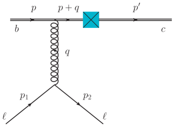
(a)  One-gluon emission from the $b$ quark

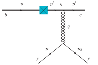
(b)  One-gluon emission from the $c$ quark

Figure 1: Tree-level continuum diagrams with a gluon exchange. A colored box represents an insertion of the flavor-changing operator.

The lattice diagrams which correspond to the continuum diagram in Fig. 1(a) are shown in Figs. 2(a) and 2(b). One-gluon emission may occur through the one-gluon vertex of the OK action as in Fig. 2(a) or through the vertex of the improved quark field as in Fig. 2(b). The small black dot attached to the current operator (cyan circle) with (without) a gluon line represents the one-gluon (zero-gluon) vertex of the improved quark fields. The charm quark part has a separate matching factor which is completely factorized from the bottom quark part.

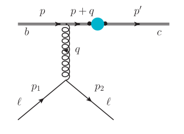
(a)  One-gluon emission from the action vertex

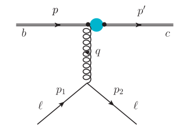
(b)  One-gluon emission from the improved quark field

Figure 2: Tree-level lattice diagrams with one-gluon exchange at the $b$-quark line. A colored circle represents an insertion of the flavor-changing current operator. The black dot without a gluon line in 2(a) and in 2(b) represents the zero-gluon vertex from the improved quark fields. The black dot with a gluon line in 2(b) represents the one-gluon emission vertex from the improved quark field.

Hence, let us focus on matching the lattice diagrams with one-gluon exchange on the $b$-quark line in Fig. 2 to the continuum diagram in Fig. 1(a). The matching condition is

$$n_{\mu}(q)\Big{[} R^{(0)}_{b}(p+q)S^{\text{lat}}_{b}(p+q)(-gt^{a})\Lambda_{\mu}(p+q,p)$$

$$+(-gt^{a})R^{(1)}_{b\mu}(p+q,p)\Big{]}\mathcal{N}_{b}(p)u^{\text{lat}}_{b}(p,s)$$

$$=S_{b}(p+q)(-gt^{a})\gamma_{\mu}\sqrt{\frac{m_{b}}{E_{b}}}u_{b}(p,s),$$ (37)

where $q$ is a four-momentum of the emitted gluon, $\mu$ is a Lorentz index, and $t^{a}$ is a generator of the SU(3) color group. $n_{\mu}(q)=2\sin(\frac{1}{2}q_{\mu})/q_{\mu}$ is the gluon line wave-function factor [30]. $S_{b}$ and $S^{\text{lat}}_{b}$ are fermion propagators of $b$ quarks in the continuum and on the lattice, respectively. Here $\Lambda_{\mu}$ is one-gluon emission vertex from the OK action for $b$ quarks. $R^{(0)}_{b}$ and $R^{(1)}_{b,\mu}$ come from the improved quark field for $b$ quarks. $R^{(1)}_{b,\mu}$ represents the one-gluon emission vertex from the improved quark field for $b$ quarks. Explicit formulas for $\Lambda_{\mu}$ and $R^{(1)}_{b,\mu}$ are given in Appendix C.

Both the spatial momentum of the external $b$ quark, $\bm{p}$, and the four-momentum of the exchanged gluon, $q$, are $\mathcal{O}(\Lambda_{\text{QCD}})$: $\bm{p},\bm{q},q_{4}\approx\Lambda_{\text{QCD}}$. They are much smaller than the physical $b$-quark mass, $m_{b}$, and the lattice cut-off scale $1/a\cong 1.6\sim 4.5\,\mathop{\rm GeV}\nolimits$. Hence, it is possible to expand both sides of Eq. (37) in power series of $q/m_{b}$, $\bm{p}/m_{b}$, $qa$, and $\bm{p}a$.

When we expand in $q$ and $\bm{p}$ on both sides of Eq. (37), a careful treatment is needed with the expansion of the heavy quark propagator, since it has pole structure. For example, in the continuum, the heavy quark propagator with momentum $p+q$ can be expanded as follows,

$$S(p+q)=\frac{m-i\gamma\cdot(p+q)}{m^{2}+(p+q)^{2}}$$

$$=\frac{m(1+\gamma_{4})-i\gamma_{4}(\tilde{p}_{4}+q_{4})-i\bm{\gamma}\cdot(\bm{p}+\bm{q})}{2im(\tilde{p}_{4}+q_{4})+(\tilde{p}_{4}+q_{4})^{2}+(\bm{p}+\bm{q})^{2}}$$

$$=\frac{1}{i(\tilde{p_{4}}+q_{4})}\frac{1+\gamma_{4}}{2}+\bigg{[}\frac{1-\gamma_{4}}{4m}-\frac{\bm{\gamma}\cdot(\bm{p}+\bm{q})}{2m(\tilde{p}_{4}+q_{4})}$$

$$+\frac{(1+\gamma_{4})(\bm{p}+\bm{q})^{2}}{4m(\tilde{p}_{4}+q_{4})^{2}}\bigg{]}+\cdots,$$ (38)

where $\tilde{p}_{4}$ is

$$\tilde{p}_{4}=p_{4}-im=i\Big{[}\frac{\bm{p}^{2}}{2m}-\frac{(\bm{p}^{2})^{2}}{8m^{2}}+\cdots\Big{]}\,.$$ (39)

Note that $(\tilde{p_{4}}+q_{4},\bm{p}+\bm{q})$ is the residual momentum of the internal heavy quark with momentum $p+q$. If we do the power series expansion as in Eq. (IV.2), then it is natural to identify each term in the matrix element in terms of HQET.

Similarly, we can apply the power series expansion to the OK-action heavy quark propagator [16]

$$S^{\text{lat}}(p+q) =\Big{[}\mu(p+q)-\cos(p_{4}+q_{4})$$

$$+i\gamma_{4}\sin(p_{4}+q_{4})+i\bm{\gamma\cdot K}(p+q)\Big{]}^{-1},$$ (40)

where

$$K_{i}(p) =\sin(p_{i})\big{[}\zeta-2c_{2}\hat{\bm{p}}^{2}-c_{1}\hat{p}^{2}_{i}\big{]},$$ (41)

$$\mu(p) =1+m_{0}+\frac{1}{2}r_{s}\zeta\hat{\bm{p}}^{2}+c_{4}\sum_{i}(\hat{p}_{i})^{4}\,.$$ (42)

Here $\hat{p}_{i}=2\sin(p_{i}/2)$. Since $\bm{p},q_{\mu}\ll 1/a,m_{0}$, we can expand the lattice propagator as in Eq. (IV.2),

$$S^{\text{lat}}(p+q) =e^{-m_{1}}\Big{[}\frac{1}{i(\tilde{p}^{\text{lat}}_{4}+q_{4})}\frac{1+\gamma_{4}}{2}+\cdots\Big{]},$$ (43)

where the ellipsis represents higher order terms. Here, note that

$$\tilde{p}^{\text{lat}}_{4} =p_{4}-im_{1}$$

$$=i\Big{[}\frac{1}{2m_{2}}\bm{p}^{2}-\frac{1}{6}w_{4}\sum_{i}p_{i}^{4}-\frac{1}{8m_{4}^{2}}\bm{p}^{4}\Big{]}+\cdots,$$ (44)

where $m_{2}$, $m_{4}$, and $w_{4}$ [16] are functions of the OK action coefficients. Their explicit formulas are given in Appendix E. In the construction of the OK action, the dispersion relation of the heavy quark is already matched to the continuum. This indicates that $m_{2}=m_{4}=m$ and $w_{4}=0$, so $\tilde{p}^{\text{lat}}_{4}=\tilde{p}_{4}$ through $\mathcal{O}(\bm{p}^{4})$.

The expansions of the external quark spinors are introduced in Eq. (29) and Eq. (30). Finally, we need to expand the lattice vertices $\Lambda_{\mu}(p+q,p)$, $R^{(0)}(p+q)$, and $R^{(1)}_{\mu}(p+q,p)$ in powers of $\bm{p}a$ and $qa$. They are analytic in $\bm{p}a$ and $qa$, and the expansion is straightforward. Comparing both sides of the expansion of the matching condition in Eq. (37), we obtain a number of constraint equations for the OK-action parameters $c_{i}$ and the current-improvement parameters $d_{i}$. These constraints are sufficient to determine all the improvement parameters $d_{i}$ through $\lambda^{3}$ order, and to put constraints on a subset of the OK-action parameters $c_{i}$. The constraints are consistent with the $c_{i}$ given in [16].

In the discussion that follows, we identify the terms in the expansion of the matching condition with contributions from (lattice and continuum) HQET. This exercise sheds light on the structure of the matching calculations and leads naturally to useful cross-checks. Let us begin with the matching calculation at leading order. First, let us choose $\mu=4$, the time direction. Then both sides of Eq. (37) are identical,

$$\frac{1}{iP_{4}}(-gt^{a})u(0,s),$$ (45)

where $P_{4}=\tilde{p}_{4}+q_{4}$. In HQET this contribution arises from one-gluon emission from the one-gluon vertex of the leading-order (LO) Lagrangian:

$$\mathcal{L}_{0}=\bar{h}^{+}[-D_{4}-m]h^{+}.$$ (46)

Second, let us choose the spatial direction $\mu=i$ ($i=1,2,3$). At leading order the right-hand side (R.H.S.) of Eq. (37) is

$$\text{R.H.S.}=$$

$$\Big{[}\frac{-i(2p_{i}+q_{i})+\epsilon_{ijk}\Sigma_{j}q_{k}}{2imP_{4}}+\frac{\gamma_{i}}{2m}\Big{]}(-gt^{a})u(0,s)\,.$$ (47)

Here the first term proportional to $1/P_{4}$ in Eq. (47) represents gluon emission by the next-to-leading-order (NLO) Lagrangian:

$$\mathcal{L}_{1}=\bar{h}^{+}\bigg{[}\frac{1}{2m}\bm{D}^{2}+\frac{i}{2m}\bm{\sigma\cdot B}\bigg{]}h^{+}\,.$$ (48)

where the definition of the matrix $\Sigma_{i}$ is in Appendix A. The second term in Eq. (47) represents gluon emission by the NLO correction term in the FWT field rotation for $b$ quarks in the flavor-changing current, given in Eq. (III).

Now, let us consider the left-hand-side (L.H.S.) of Eq. (37) with spatial direction $\mu=i$, which corresponds to the lattice part in the matching condition.

$$\text{L.H.S.}=$$

$$\Big{[}\frac{-i(2p_{i}+q_{i})}{2im_{2}P_{4}}+\frac{\epsilon_{ijk}\Sigma_{j}q_{k}}{2im_{B}P_{4}}+\frac{\gamma_{i}}{2m_{3}}\Big{]}(-gt^{a})u(0,s),$$ (49)

where $m_{2}$ and $m_{B}$ are the kinetic mass and the chromomagnetic mass at tree level, respectively:

$$\frac{1}{2m_{2}} =\frac{\zeta^{2}}{m_{0}(2+m_{0})}+\frac{r_{s}\zeta}{2(1+m_{0})}\,,$$ (50)

$$\frac{1}{2m_{B}} =\frac{\zeta^{2}}{m_{0}(2+m_{0})}+\frac{c_{B}\zeta}{2(1+m_{0})}\,,$$ (51)

and the coefficient $m_{3}$ includes a correction from the improved current

$$\frac{1}{2m_{3}} =\frac{\zeta(1+m_{0})}{m_{0}(2+m_{0})}-d_{1}\,.$$ (52)

The first two terms in Eq. (49) come from the lattice HQET Lagrangian at NLO:

$$\mathcal{L}^{\text{lat}}_{1}=\bar{h}^{+}\bigg{[}\frac{1}{2m_{2}}\bm{D}^{2}+\frac{i}{2m_{B}}\bm{\sigma\cdot B}\bigg{]}h^{+}\,,$$ (53)

which is the lattice version of Eq. (48). The matching condition requires that all the masses equal the physical mass: $m_{2}=m_{B}=m_{3}=m$. Here, $m_{2}=m_{B}=m$ is consistent with the original matching of the OK action. The relation $m_{3}=m$ reproduces Eq. (35),

$$d_{1}=\frac{\zeta(1+m_{0})}{m_{0}(2+m_{0})}-\frac{1}{2m}.$$ (54)

For the expansion through $\lambda^{3}$ order, the full expressions are given in Appendix B. The continuum part of the expansion (the R.H.S. of Eq. (37)) is given in Eq. (B) and Eq. (85). And the lattice part (the L.H.S. of Eq. (37)) is given in Eq. (B) and Eq. (87). The mass parameters $m_{i}$ and symmetry breaking parameters $w_{i}$ and $dw_{i}$ in Eq. (B) and Eq. (87) encapsulate the lattice artifacts. They are functions of the OK-action parameters and the improvement parameters $d_{i}$ of the improved quark field. The explicit formulas for $m_{i},w_{i}$, and $dw_{i}$ are given in Appendix E. The matching conditions are simply

$$m_{i}=m,\quad w_{i}=0,\qquad dw_{i}=0.$$ (55)

As we present in Appendix E, the mass parameters $m_{i}$ can be classified into two groups. The first group $M_{a}\equiv\{m_{2},m_{b},m_{E},m_{4},m_{B^{\prime}}\}$ contains the masses to be matched by the action matching. The second group $M_{b}\equiv\{m_{3},m_{\alpha E},\cdots,m_{6},m_{7}\}$ contains the masses to be matched by the current matching. We can classify the matching conditions into

$$m_{i} =m,\quad m_{i}\in M_{a},\quad w_{i}=0,\quad~{}\text{ action}$$ (56)

$$m_{i} =m,\quad m_{i}\in M_{b},\quad dw_{i}=0.\quad\text{current}$$ (57)

The matching conditions of Eq. (56) are equivalent to a subset of those for the OK action [16] : namely, the dispersion relation and background field interaction. The matching conditions of Eq. (57) determine a complete set of current improvement parameters $d_{i}$ at tree level. The explicit formulas for $d_{i}$ are summarized in Sec. VI.

In Sec. V, we will interpret the entire matching procedure in the language of HQET. Interpreting Eq. (37) in terms of the continuum and lattice HQET Feynman rules, we will show how the matching conditions can be factorized systematically.

V Cross-check by heavy quark effective theory

We have cross-checked the final results presented in Section VI in several ways. First, three researchers (Leem, Bailey, Sunkyu Lee) have done the calculation, and confirmed them. Second, when we do the matching calculation, it produces about 150 constraints on the eleven improvement parameters. The constraints also involve the coefficients in the improvement terms of the original OK action. The final results reported here are consistent with all the constraints as well as the OK action coefficients. Third, we show that the results are consistent with factorization of the matching condition in accord with the structure of contributions from HQET. Here we explain this third consistency check.

If we use HQET as a stepping stone for matching between continuum QCD ($\leftrightarrow$ continuum HQET) and lattice QCD ($\leftrightarrow$ lattice HQET), the matching condition given in Eq. (36) can be described by HQET (lattice HQET). Especially, the subdiagrams in Eq. (37) can be described by HQET Feynman rules. For the continuum, the R.H.S. of Eq. (37) is

$$\text{R.H.S.}=$$

$$\bigg{[}R^{(1)}_{\text{HQ},\mu}(p+q,p)+\sum_{n=0}^{\infty}R^{(0)}_{\text{HQ}}(p+q)\Big{(}\frac{1}{iP_{4}}\Lambda^{(0)}_{\text{HQ}}(p+q)\Big{)}^{n}$$

$$\times\frac{1}{iP_{4}}\Lambda^{(1)}_{\text{HQ},\mu}(p+q,p)\bigg{]}(-gt^{a})u(0,s),$$ (58)

where $\Lambda^{(0)}_{\text{HQ}}$ and $\Lambda^{(1)}_{\text{HQ},\mu}$ represent the zero-gluon emission and one-gluon emission vertices, respectively, which come from the HQET Lagrangian in Eq. (24). $R^{(0)}_{\text{HQ}}$ and $R^{(1)}_{\text{HQ},\mu}$ represent the zero-gluon emission and one-gluon emission vertices, respectively, which come from the FWT transformation in Eq. (III) between the QCD quark field $Q$ and the HQET field $h$. Here $n$ represents the number of perturbative insertions of higher order terms in the HQET Lagrangian with no gluon emission. The spinor $u(0,s)=\gamma_{4}u(0,s)=u_{v}(s)$ can be understood as the HQET spinor with $v=(1,\bm{0})$. The explicit formulas for $R^{(0)}_{\text{HQ}}$, $R^{(1)}_{\text{HQ},\mu}$, $\Lambda^{(0)}_{\text{HQ}}$, and $\Lambda^{(1)}_{\text{HQ},\mu}$ are given in Eq. (96)–(101) in Appendix D.

Now let us consider the lattice part. The L.H.S of Eq. (37) can be arranged as follows,

$$\text{L.H.S.}=$$

$$\bigg{[}R^{\text{lat},(1)}_{\text{HQ},\mu}(p+q,p)+\sum_{n}R^{\text{lat},(0)}_{\text{HQ}}(p+q)\Big{(}\frac{1}{iP_{4}}\Lambda^{\text{lat},(0)}_{\text{HQ}}(p+q)\Big{)}^{n}$$

$$\times\frac{1}{iP_{4}}\Lambda^{\text{lat},(1)}_{\text{HQ},\mu}(p+q,p)\bigg{]}(-gt^{a})u(0,s),$$ (59)

where $\Lambda^{\text{lat},(0)}_{\text{HQ}}$ and $\Lambda^{\text{lat},(1)}_{\text{HQ},\mu}$ are the lattice counterparts of $\Lambda^{(0)}_{\text{HQ}}$ and $\Lambda^{(1)}_{\text{HQ},\mu}$. They can be interpreted as the vertices of the HQET Lagrangian which is matched to the lattice action. We showed $1/m$ terms of this Lagrangian in Eq. (53). At order $1/m^{2}$, the lattice HQET Lagrangian is expressed in terms of a single short-distance coefficient $1/m_{E}^{2}$,

$$\mathcal{L}_{2}^{\text{lat}}=\bar{h}^{+}\bigg{[}\frac{\bm{D}\cdot\bm{E}-\bm{E}\cdot\bm{D}}{8m_{E}^{2}}+\frac{i\bm{\sigma}\cdot(\bm{D}\times\bm{E}-\bm{E}\times\bm{D})}{8m_{E}^{2}}\bigg{]}h^{+}.$$ (60)

As given in [10] and [16], the condition $m_{E}=m$ determines the chromoelectric coefficient $c_{E}$ in the action. At order $1/m^{3}$, however, tree-level matching of the four-quark matrix elements in Eq. (36) cannot give constraints on the two-gluon emission terms. In [16], the full matching of the action up to $1/m^{3}$ (or $\mathcal{\lambda}^{3}$) is presented using the two-gluon emission vertices in Compton scattering. The explicit formulas for $\Lambda^{\text{lat},(0)}_{\text{HQ}}$, $\Lambda^{\text{lat},(1)}_{\text{HQ},\mu}$ are given in Eq. (102)– (104). They are consistent with the results in [16].

In Eq. (59), $R^{\text{lat},(0)}_{\text{HQ}}$ and $R^{\text{lat},(1)}_{\text{HQ},\mu}$ represent the zero-gluon emission and one-gluon emission vertices, respectively, which are the lattice counterparts of $R^{(0)}_{\text{HQ}}$ and $R^{(1)}_{\text{HQ},\mu}$, respectively. As $R^{(0)}_{\text{HQ}}$ and $R^{(1)}_{\text{HQ},\mu}$ come from the FWT transformation between the QCD and HQET quark fields (Eq. (III)), $R^{\text{lat},(0)}_{\text{HQ}}$ and $R^{\text{lat},(1)}_{\text{HQ},\mu}$ follow from the relation between the lattice improved quarks and the HQET quarks, for example, $\Psi_{b}=\mathbf{U}_{b}^{\text{lat}}\cdot h_{b}$. We obtain this relation, in turn, from the expression for the improved field given in Eq. (III). The explicit formulas for $R^{\text{lat},(0)}_{\text{HQ}}$ and $R^{\text{lat},(1)}_{\text{HQ},\mu}$ are given in Eq. (105)–(107).

As a result, the matching condition in Eq. (37) can be factorized as matching of individual building blocks as follows,

$$\Lambda^{\text{lat},(0)}_{\text{HQ}} =\Lambda^{(0)}_{\text{HQ}}, \Lambda^{\text{lat},(1)}_{\text{HQ},\mu}=\Lambda^{(1)}_{\text{HQ},\mu}$$ (61)

$$R^{\text{lat},(0)}_{\text{HQ}} =R^{(0)}_{\text{HQ}}, R^{\text{lat},(1)}_{\text{HQ},\mu}=R^{(1)}_{\text{HQ},\mu}.$$ (62)

Here Eqs. (61) provide the matching conditions for the action. Similarly, Eqs. (62) give the matching conditions for the improved currents. We obtain $\mathbf{U}^{\text{lat}}$ as follows,

$$\mathbf{U}^{\text{lat}} =1-\frac{1}{2m_{3}}\bm{\gamma\cdot D}$$

$$+\frac{1}{4m^{2}_{\alpha_{E}}}\bm{\alpha}\cdot\bm{E}+\frac{1}{8m^{2}_{D_{\perp}^{2}}}\bm{D}^{2}+\frac{i}{8m^{2}_{sB}}\bm{\Sigma}\cdot\bm{B}$$

$$-\frac{\{\gamma_{4}D_{4},\bm{\alpha}\cdot\bm{E}\}}{8m^{3}_{\alpha_{EE}}}-\frac{3\{\bm{\gamma\cdot D},\bm{D}^{2}\}}{32m_{\gamma DD_{\perp}^{2}}^{3}}-\frac{3\{\bm{\gamma\cdot D},i\bm{\Sigma}\cdot\bm{B}\}}{32m_{5}^{3}}$$

$$-\frac{\{\bm{\gamma}\cdot\bm{D},\bm{\alpha}\cdot\bm{E}\}}{16m_{\alpha_{rE}}^{3}}+\frac{[\gamma_{4}D_{4},\bm{D}^{2}]}{16m_{6}^{3}}+\frac{[\gamma_{4}D_{4},i\bm{\Sigma}\cdot\bm{B}]}{16m_{7}^{3}}$$

$$+dw_{1}\sum_{i}\gamma_{i}D_{i}^{3}+\frac{dw_{2}}{8}[\bm{\gamma}\cdot\bm{D},\bm{D}^{2}],$$ (63)

where the coefficients $m_{i}\in M_{b}$ and $dw_{i}$ are identical to those in the expanded formulas in Eq. (B) and Eq. (87). Explicit formulas for $m_{i}$ and $dw_{i}$ are given in Appendix E.

As a result, the matching relation for the flavor-changing currents is

$$\bar{\Psi}_{Ic}\Gamma\Psi(x)_{Ib}\doteq\bar{h}_{c}\bar{\mathbf{U}}_{c}^{\text{lat}}\Gamma\mathbf{U}_{b}^{\text{lat}}h_{b}\,.$$ (64)

The matching conditions can also be written

$$\mathbf{U}^{\text{lat}}_{b}=\mathbf{U}_{b},$$ (65)

where $\mathbf{U}_{b}$ is defined in Eq. (III). This relation is identical to the matching conditions in Eq. (57).

VI Results

The final results for the improvement parameters $d_{i}$ are

$$d_{1} =\frac{\zeta(1+m_{0})}{m_{0}(2+m_{0})}-\frac{1}{2m},$$ (66)

$$d_{2} =\frac{2\zeta(1+m_{0})}{m_{0}(2+m_{0})}d_{1}-\frac{r_{s}\zeta}{2(1+m_{0})}-\frac{\zeta^{2}(1+m_{0})^{2}}{m_{0}^{2}(2+m_{0})^{2}}+\frac{1}{4m^{2}},$$ (67)

$$d_{E} =-\frac{2(1+m_{0})\zeta}{m_{0}^{2}(2+m_{0})^{2}}-\frac{(m_{0}+1)\zeta c_{E}}{m_{0}(2+m_{0})}+\frac{1}{2m^{2}},$$ (68)

$$d_{B} =d_{2}\,,$$ (69)

$$d_{r_{E}} =\frac{d_{1}d_{E}}{4},$$ (70)

$$d_{EE} =\frac{1+m_{0}}{(m_{0}^{2}+2m_{0}+2)}\Big{[}-\frac{1}{4m^{3}}+\frac{\zeta(1+m_{0})(m_{0}^{2}+2m_{0}+2)}{[m_{0}(2+m_{0})]^{3}}+\frac{\zeta c_{E}(1+m_{0})}{[m_{0}(2+m_{0})]^{2}}+\frac{(2+2m_{0}+m_{0}^{2})c_{EE}}{m_{0}(2+m_{0})}\Big{]},$$ (71)

$$d_{3} =\frac{3c_{1}+\zeta/2}{\sinh m_{1}}-d_{1},$$ (72)

$$d_{4} =\frac{\zeta^{3}(m_{0}^{3}+3m_{0}^{2}+5m_{0}+3)}{2m_{0}^{3}(2+m_{0})^{3}}+\frac{r_{s}\zeta^{2}(3m_{0}^{2}+6m_{0}+4)}{4m_{0}^{2}(2+m_{0})^{2}}+\frac{2(1+m_{0})c_{2}}{m_{0}(2+m_{0})}-\frac{(1+m_{0})^{2}\zeta^{2}}{2m_{0}^{2}(2+m_{0})^{2}}d_{1}$$

$$-\frac{r_{s}\zeta}{4(1+m_{0})}d_{1}+\frac{(1+m_{0})\zeta d_{2}}{2m_{0}(2+m_{0})}-\frac{3}{16m^{3}},$$ (73)

$$d_{5} =\frac{d_{4}}{2},$$ (74)

$$d_{6} =\frac{2(1+m_{0})}{(m_{0}^{2}+2m_{0}+2)}\Big{[}\frac{\zeta^{2}c_{E}}{4m_{0}(2+m_{0})}-\frac{\zeta c_{EE}(m_{0}^{2}+2m_{0}+2)}{2m_{0}(1+m_{0})(2+m_{0})}-\frac{d_{E}}{4}\Big{(}d_{1}-\frac{2\zeta(1+m_{0})}{m_{0}(2+m_{0})}\Big{)}-\frac{1}{24m}\Big{]},$$ (75)

$$d_{7} =d_{6}\,.$$ (76)

Here $m_{0}$ is a bare quark mass defined in Eq. (4). For numerical work, the procedure for obtaining $m_{0}$ from a hopping parameter $\kappa$ is given in Ref. [31]. Note that $m$ is equal to $m_{2}$, a kinetic quark mass defined in Eq. (108). The coefficients $c_{i}$ are parameters for the OK action.

Assuming $m_{0}a\ll 1$, we can cross-check the results against those from the Symanzik improvement program. In Table 1, we show how the coefficients $c_{i}$ of the OK action and $d_{i}$ of the current behave in the continuum limit $m_{0}a\to 0$. Here, we tune $\zeta$ so that $m_{1}=m_{2}$ and do not fix the redundant coupling $r_{s}$ to make the comparison clear. In Appendix F, we show the Symanzik improvement of the OK action through $\mathcal{O}(a^{2})$. The $\mathcal{O}(a^{2})$ study gives restricted information on $c_{i}$ and $d_{i}$. It gives terms to the next-to-leading order for $c_{B},c_{E}$, $d_{1}$ and only the leading order for $c_{1},c_{2},c_{3},c_{EE},d_{2},d_{B},d_{E}$. At higher order, it does not give any information. The results from Symanzik improvement are given in Eqs. (136)–(140) (for $c_{1},c_{2},c_{3}$, and $c_{EE}$) and Eqs. (146)–(148) (for $d_{1},d_{2},d_{B}$, and $d_{E}$). They are consistent with the expanded formulas of $c_{i}$ (the second column) and $d_{i}$ (the fourth column) in Table 1.

Table 1: Behavior of the OK action coefficients $c_{i}$ (second column) and the current improvement parameters $d_{i}$ (fourth column) in the continuum limits. Here, $\zeta$ is fixed so that $m_{1}=m_{2}$.

Coeff.	$m_{0}a\to 0$ ($m_{1}=m_{2}$)	Coeff.	$m_{0}a\to 0$ ($m_{1}=m_{2}$)
$c_{B}$	$r_{s}$	$d_{1}$	$\frac{1}{4}(1-r_{s})+\frac{1}{48}\big{(}1+3r_{s}^{2}\big{)}m_{0}a+\mathcal{O}\big{(}(m_{0}a)^{2}\big{)}$
$c_{E}$	$\frac{1}{2}(1+r_{s})+\frac{1}{12}\big{(}-2-3r_{s}+3r_{s}^{2}\big{)}m_{0}a$	$d_{2}=d_{B}$	$\frac{1}{16}\big{(}1-10r_{s}+r_{s}^{2}\big{)}+\frac{1}{96}\big{(}1+23r_{s}+27r_{s}^{2}-3r_{s}^{3}\big{)}m_{0}a$
	$+\mathcal{O}\big{(}(m_{0}a)^{2}\big{)}$		$+\mathcal{O}\big{(}(m_{0}a)^{2}\big{)}$
$c_{1}$	$-\frac{1}{6}+\frac{1}{12}\big{(}-1+5r_{s}\big{)}m_{0}a+\mathcal{O}\big{(}(m_{0}a)^{2}\big{)}$	$d_{E}$	$\frac{1}{48}\big{(}1-6r_{s}-3r_{s}^{2}\big{)}+\frac{1}{48}\big{(}-1+2r_{s}+3r_{s}^{2}\big{)}m_{0}a+\mathcal{O}\big{(}(m_{0}a)^{2}\big{)}$
$c_{2}=c_{3}$	$\frac{1}{48}\big{(}-1-6r_{s}+3r_{s}^{2}\big{)}$	$d_{r_{E}}$	$\frac{1}{768}\big{(}1-7r_{s}+3r_{s}^{2}+3r_{s}^{3}\big{)}$
	$+\frac{1}{96}\big{(}-1-r_{s}+3r_{s}^{2}-3r_{s}^{3}\big{)}m_{0}a+\mathcal{O}\big{(}(m_{0}a)^{2}\big{)}$		$+\frac{1}{9216}\big{(}-11+30r_{s}+12r_{s}^{2}-54r_{s}^{3}-9r_{s}^{4}\big{)}m_{0}a+\mathcal{O}\big{(}(m_{0}a)^{2}\big{)}$
$c_{4}$	$\frac{3}{8}r_{s}+\frac{3}{16}\big{(}r_{s}-r_{s}^{2}\big{)}m_{0}a+\mathcal{O}\big{(}(m_{0}a)^{2}\big{)}$	$d_{EE}$	$\frac{1}{384}(-1-r_{s}-3r_{s}^{2}-3r^{3})$
			${\color[rgb]{0,0,0}+\frac{1}{15360}(-9+80r_{s}+110r_{s}^{2}+120r_{s}^{3}-45r^{4}_{s})m_{0}a+\mathcal{O}\big{(}(m_{0}a)^{2}\big{)}}$
$c_{5}$	$\frac{1}{4}r_{s}+\frac{1}{8}\big{(}r_{s}-r_{s}^{2}\big{)}m_{0}a+\mathcal{O}\big{(}(m_{0}a)^{2}\big{)}$	$d_{3}$	$\frac{1}{4}(-1+5r_{s})+\frac{1}{48}\big{(}-1-3r_{s}^{2}\big{)}m_{0}a+\mathcal{O}\big{(}(m_{0}a)^{2}\big{)}$
$c_{EE}$	$\frac{1}{96}\big{(}5+6r_{s}-3r_{s}^{2}\big{)}$	$d_{4}=2d_{5}$	$\frac{1}{384}\big{(}5-31r_{s}+15r_{s}^{2}+3r_{s}^{3}\big{)}$
	${\color[rgb]{0,0,0}+\frac{1}{192}\big{(}1-9r_{s}+3r_{s}^{2}-3r_{s}^{3}\big{)}m_{0}a+\mathcal{O}\big{(}(m_{0}a)^{2}\big{)}}$		$+\frac{1}{23040}\big{(}29+570r_{s}+360r_{s}^{2}-1170r_{s}^{3}-45r_{s}^{4}\big{)}m_{0}a+\mathcal{O}\big{(}(m_{0}a)^{2}\big{)}$
		$d_{6}=d_{7}$	${\color[rgb]{0,0,0}\frac{1}{768}(-11-31r_{s}-9r_{s}^{2}+3r^{3})}$
			${\color[rgb]{0,0,0}+\frac{1}{7680}(-11+255r_{s}+235r^{2}_{s}-15r_{s}^{3})m_{0}a+\mathcal{O}\big{(}(m_{0}a)^{2}\big{)}}$

Although the $\mathcal{O}(a^{2})$ study gives partial information on $c_{i}$ and $d_{i}$, it helps us to investigate a puzzle involving $d_{E}$. The problem is that our result for $d_{E}$ given in Eq. (68) is different from that in Ref. [10]. The result for $d_{E}$ in Ref. [10] is

$$d_{E}(\text{FNAL}) =\frac{\zeta(1-c_{E})(1+m_{0}a)}{m_{0}a(2+m_{0}a)}$$

$$-\frac{\zeta(1+m_{0}a)}{m_{2}am_{0}a(2+m_{0}a)}+\frac{1}{2m_{2}^{2}a^{2}}\,,$$ (77)

which is obtained for the quarkonium system by working up to order $v^{4}$ in the power counting of NRQCD. Our result for $d_{E}$ is

$$d_{E}(\text{SWME})= -\frac{2(1+m_{0}a)\zeta}{m_{0}^{2}a^{2}(2+m_{0}a)^{2}}-\frac{\zeta c_{E}(1+m_{0}a)}{m_{0}a(2+m_{0}a)}$$

$$+\frac{1}{2m^{2}_{2}a^{2}}.$$ (78)

Here, for the comparison, we replace $m$ in Eq. (68) with $m_{2}$ without loss of generality. Taking the continuum limit ($m_{0}a\to 0$ and $|\bm{p}|/m\ll 1$) of these results gives

$$d_{E}(\text{FNAL}) =\frac{1}{16}\big{(}3-2r_{s}-r_{s}^{2}\big{)}$$

$$+ \frac{1}{48}\big{(}3-2r_{s}+3r_{s}^{2}\big{)}m_{0}a+\mathcal{O}\big{(}(m_{0}a)^{2}\big{)}\,,$$ (79)

$$d_{E}(\text{SWME}) =\frac{1}{48}\big{(}1-6r_{s}-3r_{s}^{2}\big{)}$$

$$+ \frac{1}{48}\big{(}-1+2r_{s}+3r_{s}^{2}\big{)}m_{0}a+\mathcal{O}\big{(}(m_{0}a)^{2}\big{)}\,.$$ (80)

As we can see, even the leading-order terms of $d_{E}(\text{FNAL})$ and $d_{E}(\text{SWME})$ are different from each other. Our result for the leading term in $d_{E}(\text{SWME})$ is consistent with that from Symanzik improvement, given in Eq. (148). We have not found any problem in the derivation of $d_{E}(\text{FNAL})$ in Ref. [10]. Hence, we do not yet understand the source of the difference between $d_{E}(\text{FNAL})$ and $d_{E}(\text{SWME})$. However, Andreas Kronfeld, one of the authors of Ref. [10] (FNAL) has derived $d_{E}$ independently, following our Feynman diagram method, and produced results consistent with $d_{E}(\text{SWME})$ [32]. The Hamiltonian method that produced $d_{E}(\text{FNAL})$ is under investigation [32].

Next, let us consider the static limit. In the Fermilab method [10, 16], lattice discretization error is bounded in the static limit. If we set the improvement parameters to zero: $d_{j}=0$ or the action coefficients to zero : $c_{j}=0$, the discretization error comes from mismatches between lattice mass-like terms $m_{i}(d_{j}=0,c_{j}=0)$ and the physical mass $m$, or from pure lattice artifacts $w_{i}$ and $dw_{i}$. For example, if one does not introduce the second order improvement parameter $d_{2}$ in the improved current, the discretization error propagates from the discrepancy between $1/(8m^{2})$ and $1/(8m_{D_{\perp}}^{2})|_{d_{2}=0}$ (with $d_{2}$ = 0 in Eq. (116)). Likewise, if one does not introduce the chromoelectric term in the action ($c_{E}=0$), the discretization error will propagate from the discrepancy between $1/(4m^{2})$ and $1/(4m_{E}^{2})|_{c_{E}=0}$. As we can see in Eq. (109) and Eq. (116), $1/4m_{E}^{2}|_{c_{E}=0}$ and $1/(8m_{D_{\perp}}^{2})|_{d_{2}=0}$ behave smoothly as $am_{0}\to\infty$. The other terms of the action matching in Eq. (108) - Eq. (113) and those in the current matching in Eq. (114) - Eq. (125) have the same property. The smooth behavior makes it possible to control the discretization errors even for heavy quarks with $m_{Q}a>1$.

VII Conclusion

The goal of this paper is to improve the current operators through $\lambda^{3}$ order in HQET power counting, the same level as the OK action. These improved currents can be used to calculate the semi-leptonic form factors for the $\bar{B}\to D^{\ast}\ell\bar{\nu}$, $\bar{B}\to D\ell\bar{\nu}$, $\bar{B}\to\pi\ell\bar{\nu}$, and $\bar{B}_{s}\to K\ell\bar{\nu}$ decays and the decay constants $f_{B}$ and $f_{D}$. Our final results for the improvement coefficients $d_{i}$ are presented in Section VI.

We adopt the concept of the improved quark field in Ref. [10] and extend it to $\mathcal{O}(\lambda^{3})$ at tree level. We find that one needs to add seven more terms of higher dimension and corresponding improvement parameters at order $\lambda^{3}$ to Eq. (A.17) of Ref. [10]. With one exception (the $d_{3}$ term), the higher dimension lattice operators are lattice versions of operators in the continuum FWT transformation. The $d_{3}$ operator is required to compensate for rotation-symmetry-breaking contributions from the normalized spinors of the OK action. Thus, we need eleven improvement terms in total.

Our matching conditions in Eq. (33) and Eq. (37) determine the improvement parameters uniquely. Our final results given in Section VI have been checked in several ways. First, three individuals (Jaehoon Leem, Jon Bailey, Sunkyu Lee) have performed the calculation and cross-checked the results against one another. Second, the matching condition provides about 150 self-consistent constraint equations. The constraint equations from the temporal and spatial components of the one-gluon emission vertex are consistent with each other. The constraint equations from the zero-gluon emission vertex are also consistent with those from two-quark matrix elements. As a by-product, the matching condition reproduces the constraint equations for the zero-gluon and one-gluon emission vertices of the OK action. In addition, the matching condition can be expressed in terms of contributions from continuum HQET (Eq. (58)) and lattice HQET (Eq. (59)). For the quark-level matrix elements we match, the vertices of the continuum currents and action are in one-to-one correspondence with the vertices of the lattice currents and action (Eq. (61) and Eq. (62)). This one-to-one mapping provides another cross-check on the final results in Section VI. At the same time, we note that Eq. (64) is established for the quark-level matrix elements we match by constructing the rotation matrix from the ansatz for the improved field.

There remains a puzzle involving $d_{E}$. Our result (SWME) is given in Eq. (78). At present, there is another result (FNAL) for $d_{E}$ available in Ref. [10] which is presented in Eq. (77). They are different from each other even at leading order in the continuum limit. To check the validity of our result, we have performed Symanzik improvement assuming $m_{0}a\ll 1$ and $|\bm{p}|/m\ll 1$. We find the result is consistent with our result for $d_{E}$. However, we have not found any problem with the derivation of $d_{E}$ in Ref. [10]. Therefore, this issue needs further investigation.

Appendix A Notation

We use the same signature for the $\gamma$-matrices as in Ref. [10]. The representation for Euclidean gamma matrices is

$$\bm{\gamma}=\begin{pmatrix}~{}0&\bm{\sigma}~{}\\ ~{}\bm{\sigma}&0~{}\end{pmatrix},\qquad\gamma_{4}=\begin{pmatrix}~{}1&0~{}\\ ~{}0&-1~{}\end{pmatrix},$$ (81)

where $\bm{\sigma}$ are Pauli matrices. The $\gamma$-matrices satisfy the Clifford algebra:

$$\{\gamma_{\mu},\gamma_{\nu}\} =2\delta_{\mu\nu}$$ (82)

The remaining definitions are

$$\bm{\alpha}=\begin{pmatrix}~{}0&\bm{\sigma}\\ -\bm{\sigma}&0~{}\end{pmatrix},\qquad\bm{\Sigma}=\begin{pmatrix}~{}\bm{\sigma}&0~{}\\ ~{}0&\bm{\sigma}~{}\end{pmatrix},$$ (83)

where $\alpha_{i}=\gamma_{4}\gamma_{i}$ and $\Sigma_{k}=-\frac{i}{4}\epsilon_{ijk}[\gamma_{i},\gamma_{j}]$.

Appendix B Matching sub-diagrams

The expansion of the right-hand side (continuum) of Eq. (37) through third order in $\lambda$ is as follows,

R.H.S $$(\mu=4)=\Bigg{[}\frac{1}{iP_{4}}-\frac{\bm{\gamma\cdot(p+q)}}{2mP_{4}}+\frac{(\bm{p}+\bm{q})^{2}}{2mP_{4}^{2}}-\frac{i\bm{\gamma\cdot q}}{4m^{2}}+\epsilon_{ijk}\Sigma_{i}\frac{q_{j}p_{k}}{4m^{2}P_{4}}+\frac{i\big{(}\bm{p}^{2}+2\bm{q}\cdot(\bm{p}+\bm{q})\big{)}}{8m^{2}P_{4}}-\frac{i\bm{\gamma}\cdot(\bm{p}+\bm{q})(\bm{p}+\bm{q})^{2}}{4m^{2}P_{4}^{2}}$$

$$+\frac{i((\bm{p}+\bm{q})^{2})^{2}}{4m^{2}P_{4}^{3}}-\frac{\bm{q}\cdot(\bm{p}+\bm{q})}{8m^{3}}+\frac{\bm{\gamma}\cdot\bm{q}}{8m^{3}}q_{4}+\epsilon_{ijk}\Sigma_{i}\frac{iq_{j}p_{k}}{8m^{3}}+\frac{\bm{\gamma}\cdot(\bm{p}+\bm{q})\bm{p}^{2}}{16m^{3}P_{4}}+\frac{\bm{\gamma}\cdot(\bm{p}+2\bm{q})(\bm{p}+\bm{q})^{2}}{8m^{3}P_{4}}$$

$$-\frac{(\bm{p}+\bm{q})^{2}\big{(}3(\bm{p}+\bm{q})^{2}+\bm{q}^{2}\big{)}}{16m^{3}P_{4}^{2}}+\epsilon_{ijk}\Sigma_{i}\frac{iq_{j}p_{k}(\bm{p}+\bm{q})^{2}}{8m^{3}P_{4}^{2}}+\frac{\bm{\gamma}\cdot(\bm{p}+\bm{q})\big{(}(\bm{p}+\bm{q})^{2}\big{)}^{2}}{8m^{3}P_{4}^{3}}-\frac{((\bm{p}+\bm{q})^{2})^{3}}{8m^{3}P_{4}^{4}}\Bigg{]}(-gt^{a})u(0,s),$$ (84)

R.H.S $$(\mu=i)=\Bigg{[}\frac{1}{2m}\gamma_{i}-\frac{(2p_{i}+q_{i})+\epsilon_{ijk}i\Sigma_{j}q_{k}}{2mP_{4}}+\frac{iq_{4}}{4m^{2}}\gamma_{i}-\frac{i(p_{i}+q_{i})}{4m^{2}}+\epsilon_{ijk}\Sigma_{j}\frac{q_{k}+p_{k}}{4m^{2}}+\frac{i(\bm{p}+\bm{q})\cdot\bm{q}}{4m^{2}P_{4}}\gamma_{i}+\frac{i\bm{\gamma}\cdot(\bm{p}+\bm{q})p_{i}}{4m^{2}P_{4}}$$

$$+\frac{i\bm{\gamma}\cdot\bm{p}(p_{i}+q_{i})}{4m^{2}P_{4}}-\epsilon_{ijk}\gamma_{5}\frac{iq_{j}p_{k}}{4m^{2}P_{4}}+\epsilon_{ijk}\frac{\Sigma_{j}q_{k}(\bm{p}+\bm{q})^{2}}{4m^{2}P_{4}^{2}}-i(2p_{i}+q_{i})\frac{(\bm{p}+\bm{q})^{2}}{4m^{2}P_{4}^{2}}+\frac{(p_{i}+q_{i})q_{4}}{8m^{3}}-\frac{q_{4}^{2}}{8m^{3}}\gamma_{i}-\frac{\bm{p}^{2}}{8m^{3}}\gamma_{i}$$

$$-\frac{3(\bm{p}+\bm{q})^{2}+\bm{q}^{2}}{16m^{3}}\gamma_{i}-\frac{p_{i}\bm{\gamma}\cdot(\bm{p}+\bm{q})}{8m^{3}}-\frac{(p_{i}+q_{i})\bm{\gamma}\cdot\bm{p}}{8m^{3}}+\epsilon_{ijk}\Sigma_{j}\frac{i(p_{k}+q_{k})q_{4}}{8m^{3}}+\epsilon_{ijk}\gamma_{5}\frac{q_{j}p_{k}}{8m^{3}}+\frac{(4p_{i}+q_{i})\bm{p}^{2}}{16m^{3}P_{4}}$$

$$+\frac{(3p_{i}+2q_{i})(\bm{p}+\bm{q})^{2}}{8m^{3}P_{4}}+\epsilon_{ijk}\Sigma_{j}\frac{i(q_{k}-2p_{k})\bm{p}^{2}}{16m^{3}P_{4}}+\epsilon_{ijk}\Sigma_{j}\frac{i(p_{k}+2q_{k})(\bm{p}+\bm{q})^{2}}{8m^{3}P_{4}}-\frac{p_{i}\bm{\gamma\cdot}(\bm{p}+\bm{q})(\bm{p}+\bm{q})^{2}}{8m^{3}P_{4}^{2}}$$

$$-\frac{(p_{i}+q_{i})\bm{\gamma\cdot}\bm{p}(\bm{p}+\bm{q})^{2}}{8m^{3}P_{4}^{2}}-\frac{\bm{q}\cdot(\bm{p}+\bm{q})(\bm{p}+\bm{q})^{2}}{8m^{3}P_{4}^{2}}\gamma_{i}+\epsilon_{ijk}\gamma_{5}\frac{q_{j}p_{k}(\bm{p}+\bm{q})^{2}}{8m^{3}P_{4}^{2}}+\epsilon_{ijk}\Sigma_{j}\frac{iq_{k}\big{(}(\bm{p}+\bm{q})^{2}\big{)}^{2}}{8m^{3}P_{4}^{3}}$$

$$+\frac{(2p_{i}+q_{i})\big{(}(\bm{p}+\bm{q})^{2}\big{)}^{2}}{8m^{3}P_{4}^{3}}\Bigg{]}(-gt^{a})u(0,s).$$ (85)

And the left-hand side (lattice) is

L.H.S $$(\mu=4)=\Bigg{[}\frac{1}{iP_{4}}-\frac{\bm{\gamma\cdot(p+q)}}{2m_{3}P_{4}}+\frac{(\bm{p}+\bm{q})^{2}}{2m_{2}P_{4}^{2}}-\frac{i\bm{\gamma}\cdot\bm{q}}{4m^{2}_{\alpha_{E}}}+\frac{i(\bm{p}+\bm{q})^{2}}{8m_{D^{2}_{\perp}}^{2}P_{4}}+\frac{i\bm{q}^{2}+2\epsilon_{ijk}\Sigma_{i}q_{j}p_{k}}{8m_{E}^{2}P_{4}}-\frac{i\bm{\gamma}\cdot(\bm{p}+\bm{q})(\bm{p}+\bm{q})^{2}}{4m_{2}m_{3}P_{4}^{2}}$$

$$+\frac{i\big{(}(\bm{p}+\bm{q})^{2}\big{)}^{2}}{4m^{2}_{2}P_{4}^{3}}-\frac{\bm{q}^{2}-2i\epsilon_{ijk}\Sigma_{i}q_{j}p_{k}}{16m^{3}_{\alpha_{rE}}}-\frac{\bm{q}\cdot(2\bm{p}+\bm{q})}{16m_{6}^{3}}+\frac{\bm{\gamma}\cdot\bm{q}}{8m^{3}_{\alpha_{EE}}}q_{4}+\frac{\bm{\gamma}\cdot(\bm{p}+\bm{q})\bm{p}^{2}-\bm{\gamma}\cdot({\bm{p}-\bm{q})}(\bm{p}+\bm{q})^{2}}{16m_{3}m_{E}^{2}P_{4}}$$

$$+\frac{3\bm{\gamma}\cdot(\bm{p}+\bm{q})(\bm{p}+\bm{q})^{2}}{16m^{3}_{\gamma DD_{\perp}^{2}}P_{4}}-\frac{(\bm{p}+\bm{q})^{2}\big{(}\bm{q}^{2}-2i\epsilon_{ijk}\Sigma_{i}q_{j}p_{k}\big{)}}{16m_{2}m_{E}^{2}P_{4}^{2}}-\frac{\big{(}(\bm{p}+\bm{q})^{2}\big{)}^{2}}{16m_{2}m^{2}_{D^{2}_{\perp}}P_{4}^{2}}-\frac{\big{(}(\bm{p}+\bm{q})^{2}\big{)}^{2}}{8m_{4}^{3}P_{4}^{2}}-\frac{dw_{1}}{6P_{4}}\sum_{i}\gamma_{i}(p_{i}+q_{i})^{3}$$

$$-\frac{w_{4}}{6P_{4}^{2}}\sum_{i}(p_{i}+q_{i})^{4}+\frac{\bm{\gamma}\cdot(\bm{p}+\bm{q})}{8m_{2}^{2}m_{3}P_{4}^{3}}\big{(}(\bm{p}+\bm{q})^{2}\big{)}^{2}-\frac{\big{(}(\bm{p}+\bm{q})^{2}\big{)}^{3}}{8m^{3}_{2}P_{4}^{4}}\Bigg{]}(-gt^{a})u(0,s),$$ (86)

L.H.S $$(\mu=i)=\Bigg{[}\frac{1}{2m_{3}}\gamma_{i}-\frac{(2p_{i}+q_{i})}{2m_{2}P_{4}}-\frac{i\epsilon_{ijk}\Sigma_{j}q_{k}}{2m_{B}P_{4}}+\frac{iq_{4}}{4m_{\alpha_{E}}^{2}}\gamma_{i}-i\frac{2p_{i}+q_{i}}{8m_{D^{2}_{\perp}}^{2}}+\epsilon_{ijk}\Sigma_{j}\frac{q_{k}}{8m_{sB}^{2}}-\frac{i\big{(}q_{i}+i\epsilon_{ijk}\Sigma_{j}(2p_{k}+q_{k})\big{)}}{8m_{E}^{2}}$$

$$+\frac{i(\bm{p}+\bm{q})\cdot\bm{q}\gamma_{i}}{4m_{3}m_{B}P_{4}}+\frac{i(2p_{i}+q_{i})(\bm{p}+\bm{q})\cdot\bm{\gamma}}{4m_{3}m_{2}P_{4}}-\frac{i(p_{i}+q_{i})\bm{q}\cdot\bm{\gamma}}{4m_{3}m_{B}P_{4}}-i\epsilon_{ijk}\frac{q_{j}p_{k}\gamma_{5}}{4m_{3}m_{B}P_{4}}+\epsilon_{ijk}\Sigma_{j}\frac{q_{k}(\bm{p}+\bm{q})^{2}}{4m_{B}m_{2}P_{4}^{2}}$$

$$-\frac{i(2p_{i}+q_{i})(\bm{p}+\bm{q})^{2}}{4m_{2}^{2}P_{4}^{2}}-\frac{q_{4}^{2}}{8m^{3}_{\alpha_{EE}}}\gamma_{i}+\frac{q_{4}(2p_{i}+q_{i})}{16m_{6}^{3}}+\frac{q_{i}q_{4}}{16m^{3}_{\alpha_{rE}}}-\frac{3\big{(}(\bm{p}+\bm{q})^{2}+\bm{p}^{2}\big{)}}{32m_{\gamma DD^{2}_{\perp}}^{3}}\gamma_{i}-\frac{3\bm{q}^{2}}{32m_{5}^{3}}\gamma_{i}$$

$$-\frac{(\bm{p}+\bm{q})\cdot(2\bm{p}+\bm{q})}{16m_{3}m_{E}^{2}}\gamma_{i}+\frac{3q_{i}\bm{\gamma}\cdot\bm{q}}{32m_{5}^{3}}-\frac{3(2p_{i}+q_{i})\bm{\gamma}\cdot(2\bm{p}+\bm{q})}{32m_{\gamma DD_{\perp}^{2}}^{3}}+\frac{(2p_{i}+q_{i})\bm{\gamma}\cdot\bm{p}+p_{i}\bm{\gamma}\cdot\bm{q}}{16m_{3}m_{E}^{2}}+i\epsilon_{ijk}\Sigma_{j}\frac{q_{4}q_{k}}{16m_{7}^{3}}$$

$$+i\epsilon_{ijk}\Sigma_{j}\frac{q_{4}(2p_{k}+q_{k})}{16m_{\alpha_{rE}}^{3}}+\epsilon_{ijk}\gamma_{5}\frac{3q_{j}p_{k}}{16m_{5}^{3}}-\epsilon_{ijk}\gamma_{5}\frac{q_{j}p_{k}}{16m_{E}^{2}m_{3}}+\frac{dw_{2}}{8}\big{(}-\bm{q}\cdot(2\bm{p}+\bm{q})\gamma_{i}+\bm{\gamma}\cdot\bm{q}(2p_{i}+q_{i})\big{)}$$

$$+\frac{1}{6}dw_{1}\gamma_{i}(3p_{i}^{2}+3p_{i}q_{i}+q_{i}^{2})+\frac{(2p_{i}+q_{i})((\bm{p}+\bm{q})^{2}+\bm{p}^{2})}{8m_{4}^{3}P_{4}}+\frac{\bm{q}\cdot(2\bm{p}+\bm{q})q_{i}}{16m_{2}m_{E}^{2}P_{4}}+\frac{(2p_{i}+q_{i})(\bm{p}+\bm{q})^{2}}{16m_{D_{\perp}^{2}}^{2}m_{2}P_{4}}$$

$$+i\epsilon_{ijk}\Sigma_{j}\frac{q_{k}(\bm{p}^{2}+(\bm{p}+\bm{q})^{2})}{8m_{B^{\prime}}^{3}P_{4}}+i\epsilon_{ijk}\Sigma_{j}\frac{q_{k}(\bm{p}+\bm{q})^{2}}{16m_{D^{2}_{\perp}}^{2}m_{B}P_{4}}+i\epsilon_{ijk}\Sigma_{j}\frac{(2p_{k}+q_{k})\big{(}\bm{q}\cdot(2\bm{p}+\bm{q})\big{)}}{16m_{2}m^{2}_{E}P_{4}}-\frac{w_{B}}{8P_{4}}(p_{i}\bm{q}^{2}-q_{i}\bm{p}\cdot\bm{q})$$

$$-\frac{w_{B}}{16P_{4}}i\epsilon_{ijk}\Sigma_{j}q_{k}\bm{q}^{2}+\frac{w_{4}}{6P_{4}}(2p_{i}+q_{i})\big{(}(p_{i}+q_{i})^{2}+p_{i}^{2}\big{)}+\frac{w_{B}}{8P_{4}}i\epsilon_{ijk}q_{j}p_{k}\bm{\Sigma}\cdot(2\bm{p}+\bm{q})+\frac{w^{\prime}_{B}}{12P_{4}}i\epsilon_{ijk}\Sigma_{j}q_{k}(q_{i}^{2}+q_{k}^{2})$$

$$+\frac{(w_{4}+w^{\prime}_{4})}{12P_{4}}i\epsilon_{ijk}\Sigma_{j}q_{k}\Big{(}(3p_{i}^{2}+3p_{i}q_{i}+q_{i}^{2})+(3p_{k}^{2}+3p_{k}q_{k}+q_{k}^{2})\Big{)}-\frac{(2p_{i}+q_{i})(\bm{p}+\bm{q})\cdot\bm{\gamma}(\bm{p}+\bm{q})^{2}}{8m_{3}m_{2}^{2}P_{4}^{2}}$$

$$+\frac{(p_{i}+q_{i})\bm{q}\cdot\bm{\gamma}(\bm{p}+\bm{q})^{2}}{8m_{3}m_{2}m_{B}P_{4}^{2}}-\frac{\bm{q}\cdot(\bm{p}+\bm{q})(\bm{p}+\bm{q})^{2}\gamma_{i}}{8m_{3}m_{2}m_{B}P_{4}^{2}}+\epsilon_{ijk}\gamma_{5}\frac{q_{j}p_{k}(\bm{p}+\bm{q})^{2}}{8m_{3}m_{2}m_{B}P_{4}^{2}}+i\epsilon_{ijk}\Sigma_{j}\frac{q_{k}((\bm{p}+\bm{q})^{2})^{2}}{8m_{2}^{2}m_{B}P_{4}^{3}}$$

$$+\frac{(2p_{i}+q_{i})\big{(}(\bm{p}+\bm{q})^{2}\big{)}^{2}}{8m_{2}^{3}P_{4}^{3}}\Bigg{]}(-gt^{a})u(0,s).$$ (87)

Appendix C Lattice Feynman rules

The one-gluon vertices of the OK action from Ref. [16] are as follows (set $a=1$),

$$\Lambda_{4}(p+q,p)=\gamma_{4}\cos\big{(}p_{4}+\frac{1}{2}q_{4}\big{)} -i\sin\big{(}p_{4}+\frac{1}{2}q_{4}\big{)}+\frac{i}{2}c_{E}\zeta\sum_{i}\alpha_{i}\sin q_{i}\cos\frac{1}{2}q_{4}$$

$$+c_{EE}\sum_{i}\gamma_{i}\cdot\sin q_{i}\big{[}\sin(p+q)_{4}-\sin p_{4}\big{]}\cos\frac{1}{2}q_{4},$$ (88)

$$\Lambda_{i}(p+q,p) =\zeta\gamma_{i}\cos\big{(}p_{i}+\frac{1}{2}q_{i}\big{)}-ir_{s}\zeta\sin\big{(}p_{i}+\frac{1}{2}q_{i})-\frac{i}{2}c_{E}\zeta\alpha_{i}\sin q_{4}\cos\frac{1}{2}q_{i}-\frac{1}{2}c_{B}\zeta\epsilon_{irm}\Sigma_{m}\sin q_{r}\cos\frac{1}{2}q_{i}$$

$$-c_{2}\bigg{[}\gamma_{i}\cos(p_{i}+\frac{1}{2}q_{i})\sum_{j}4\big{[}\sin^{2}\frac{1}{2}(p_{j}+q_{j})+\sin^{2}\frac{1}{2}p_{j}\big{]}+2\sin(p_{i}+\frac{1}{2}q_{i})\sum_{j}\gamma_{j}\big{[}\sin(p_{j}+q_{j})+\sin p_{j}\big{]}\bigg{]}$$

$$-\frac{1}{2}c_{1}\gamma_{i}\bigg{[}4\cos(p_{i}+\frac{1}{2}q_{i})\big{[}\sin^{2}\frac{1}{2}(p_{i}+q_{i})+\sin^{2}\frac{1}{2}p_{i}\big{]}+2\sin(p_{i}+\frac{1}{2}q_{i})\big{[}\sin(p_{i}+q_{i})+\sin p_{i}\big{]}\bigg{]}$$

$$+c_{3}\cos\frac{1}{2}q_{i}\bigg{[}\sum_{j}\gamma_{j}\sin q_{j}\big{[}\sin(p_{i}+q_{i})-\sin p_{i}\big{]}-\gamma_{i}\sum_{j}\sin q_{j}\big{[}\sin(p_{j}+q_{j})-\sin p_{j}\big{]}$$

$$\qquad\qquad\qquad-\gamma_{4}\gamma_{5}\sum_{r,m}\epsilon_{irm}\sin q_{r}\big{[}\sin(p_{m}+q_{m})+\sin p_{m}\big{]}\bigg{]}$$

$$-c_{EE}\gamma_{i}\sin q_{4}\big{[}\sin(p_{4}+q_{4})-\sin p_{4}\big{]}\cos\frac{1}{2}q_{i}-8ic_{4}\sin(p_{i}+\frac{1}{2}q_{i})\big{[}\sin^{2}\frac{1}{2}(p_{i}+q_{i})+\sin^{2}\frac{1}{2}p_{i}\big{]}$$

$$-4c_{5}\epsilon_{irm}\Sigma_{m}\sin q_{r}\cos\frac{1}{2}q_{i}\Big{[}\sum_{j}\big{[}\sin^{2}\frac{1}{2}\big{(}p_{j}+q_{j})+\sin^{2}\frac{1}{2}p_{j}\big{]}-\big{[}\sin^{2}\frac{1}{2}\big{(}p_{m}+q_{m}\big{)}+\sin^{2}\frac{1}{2}p_{m}\big{]}\Big{]}\,.$$ (89)

The zero-gluon vertex of the improved quark field is as follows,

$$R^{(0)}(p+q) =e^{m_{1}/2}\Bigg{[}1+id_{1}\sum_{j}\gamma_{j}\sin(p_{j}+q_{j})-2d_{2}\sum_{j}\sin^{2}\frac{1}{2}(p_{j}+q_{j})$$

$$-\frac{2}{3}id_{3}\sum_{j}\gamma_{j}\sin(p_{j}+q_{j})\sin^{2}\frac{1}{2}(p_{j}+q_{j})-4id_{4}\sum_{j,k}\gamma_{j}\sin(p_{j}+q_{j})\sin^{2}\frac{1}{2}(p_{k}+q_{k})\Bigg{]}\,.$$ (90)

The one-gluon vertices of the improved quark field are as follows,

$$R^{(1)}_{4}(p+q,p)=e^{m_{1}/2} \cos\frac{1}{2}q_{4}\gamma_{4}\Bigg{[}\frac{i}{2}d_{E}\sum_{j}\gamma_{j}\sin q_{j}-d_{EE}\gamma_{4}\sum_{j}\gamma_{j}\sin q_{j}\big{[}\sin(p_{4}+q_{4})-\sin p_{4}\big{]}$$

$$+d_{r_{E}}\sum_{j}\sin q_{j}\big{[}\sin(p_{j}+q_{j})-\sin p_{j}\big{]}-id_{r_{E}}\sum_{j,l,m}\epsilon_{jlm}\Sigma_{j}\sin q_{l}\big{[}\sin(p_{m}+q_{m})+\sin p_{m}\big{]}\Bigg{]}$$

$$-4e^{m_{1}/2} d_{6}\cos(p_{4}+\frac{1}{2}q_{4})\gamma_{4}\sum_{j}\big{[}\sin^{2}\frac{1}{2}(p_{j}+q_{j})-\sin^{2}\frac{1}{2}p_{j}\big{]}\,,$$ (91)

$$R^{(1)}_{i}(p+q,p)=e^{m_{1}/2} \Bigg{[}-d_{1}\gamma_{i}\cos(p_{i}+\frac{1}{2}q_{i})-id_{2}\sin(p_{i}+\frac{1}{2}q_{i})-\frac{1}{2}d_{B}\sum_{r,m}\epsilon_{irm}\Sigma_{m}\sin q_{r}\cos\frac{1}{2}q_{i}$$

$$-\frac{i}{2}d_{E}\gamma_{4}\gamma_{i}\cos\frac{1}{2}q_{i}\sin q_{4}+d_{r_{E}}\sum_{r,m}i\epsilon_{irm}\Sigma_{m}\gamma_{4}\sin q_{4}\big{[}\sin(p_{r}+q_{r})+\sin p_{r}\big{]}\cos\frac{1}{2}q_{i}$$

$$-d_{r_{E}}\gamma_{4}\sin q_{4}\big{[}\sin(p_{i}+q_{i})-\sin p_{i}\big{]}\cos\frac{1}{2}q_{i}+d_{EE}\gamma_{i}\sin q_{4}\big{[}\sin(p_{4}+q_{4})-\sin p_{4}\big{]}\cos\frac{1}{2}q_{i}$$

$$+\frac{1}{2}d_{4}\bigg{[}\gamma_{i}\cos(p_{i}+\frac{1}{2}q_{i})\sum_{j}4\big{[}\sin^{2}\frac{1}{2}(p_{j}+q_{j})+\sin^{2}\frac{1}{2}p_{j}\big{]}+2\sin(p_{i}+\frac{1}{2}q_{i})\sum_{j}\gamma_{j}\big{[}\sin(p_{j}+q_{j})+\sin p_{j}\big{]}\bigg{]}$$

$$+\frac{1}{12}d_{3}\gamma_{i}\bigg{[}4\cos(p_{i}+\frac{1}{2}q_{i})\big{[}\sin^{2}\frac{1}{2}(p_{i}+q_{i})+\sin^{2}\frac{1}{2}p_{i}\big{]}+2\sin(p_{i}+\frac{1}{2}q_{i})\big{[}\sin(p_{i}+q_{i})+\sin p_{i}\big{]}\bigg{]}$$

$$+d_{5}\cos\frac{1}{2}q_{i}\Big{[}-\sum_{j}\gamma_{j}\sin q_{j}\big{[}\sin(p_{i}+q_{i})-\sin p_{i}\big{]}+\gamma_{i}\sum_{j}\sin q_{j}\big{[}\sin(p_{j}+q_{j})-\sin p_{j}\big{]}\Big{]}$$

$$+d_{5}\cos\frac{1}{2}q_{i}\gamma_{4}\gamma_{5}\sum_{r,m}\epsilon_{irm}\sin q_{r}\big{[}\sin(p_{m}+q_{m})+\sin p_{m}\big{]}$$

$$+2d_{6}\gamma_{4}\big{[}\sin(p_{4}+q_{4})-\sin p_{4}\big{]}\sin(p_{i}+\frac{1}{2}q_{i})$$

$$-i\sum_{r,m}\epsilon_{irm}d_{7}\big{[}\sin(p_{4}+q_{4})-\sin p_{4}\big{]}\cos\frac{1}{2}q_{i}\sin q_{r}\Sigma_{m}\gamma_{4}\Bigg{]}\,.$$ (92)

The factor for the external incoming fermion with momentum $p$ and spin $s$ is given by $\mathcal{N}(p)u^{\text{lat}}(p,s)$ with the normalization factor $\mathcal{N}(p)$ and the spinor $u^{\text{lat}}(p,s)$ as follows [10, 16],

$$\mathcal{N}(p) =\bigg{(}\frac{\mu(p)-\cosh E}{\mu(p)\sinh E}\bigg{)}^{1/2},$$ (93)

$$u^{\text{lat}}(p,s) =\frac{\mu(p)-\cosh E+\sinh E-i\bm{\gamma\cdot K}}{\sqrt{2(\mu(p)-\cosh E)(\mu(p)-\cosh E+\sinh E)}}u(0,s),$$ (94)

where $\mu(p)$ is given in Eq. (42) and $u(0,s)$ is a constant spinor which satisfies $\gamma_{4}u(0,s)=u(0,s)$. Here, $\mathcal{N}(p)$ corresponds to $\sqrt{\frac{m}{E}}$ and $u^{\text{lat}}(p,s)$ corresponds to the continuum spinor as follows,

$$u(p,s)=\frac{m+E-i\bm{\gamma\cdot p}}{\sqrt{2m(m+E)}}u(0,s).$$ (95)

Appendix D HQET Feynman rules

The zero-gluon vertex of the HQET Lagrangian is as follows,

$$\Lambda^{(0)}_{\text{HQ}}(p)=-\frac{1}{2m}\bm{p}^{2}+\frac{1}{8m^{3}}\big{(}\bm{p}^{2}\big{)}^{2}.$$ (96)

The one-gluon vertices of the HQET Lagrangian are as follows,

$$\Lambda^{(1)}_{\text{HQ},4}(p+q,p) =\Big{[}1-\frac{\bm{q}^{2}-2i\epsilon_{ijk}q_{i}p_{j}\Sigma_{k}}{8m^{2}}\Big{]},$$ (97)

$$\Lambda^{(1)}_{\text{HQ},i}(p+q,p) =\Big{[}-\frac{i}{2m}(2p_{i}+q_{i})+\frac{1}{2m}\epsilon_{ijk}\Sigma_{j}q_{k}+\frac{q_{4}}{8m^{2}}\big{(}q_{i}+i\epsilon_{ijk}\Sigma_{j}(2p_{k}+q_{k})\big{)}+\frac{i(2p_{i}+q_{i})}{8m^{3}}\big{(}(\bm{p}+\bm{q})^{2}+\bm{p}^{2}\big{)}$$

$$\qquad-\frac{1}{8m^{3}}\epsilon_{ijk}\Sigma_{j}q_{k}\big{(}(\bm{p}+\bm{q})^{2}+\bm{p}^{2}\big{)}\Big{]},$$ (98)

The zero-gluon vertex from Eq. (III) is as follows,

$$R^{(0)}_{\text{HQ}}(p)=1 -\frac{i}{2m}\bm{\gamma}\cdot\bm{p}-\frac{1}{8m^{2}}\bm{p}^{2}+\frac{3i\bm{\gamma}\cdot\bm{p}}{16m^{3}}\bm{p}^{2}.$$ (99)

The one-gluon vertices from Eq. (III) are as follows,

$$R^{(1)}_{\text{HQ},4}(p+q,p) =-\frac{i}{4m^{2}}\bm{\gamma}\cdot\bm{q}+\frac{q_{4}}{8m^{3}}\bm{\gamma}\cdot\bm{q}-\frac{1}{16m^{3}}\big{(}\bm{q}^{2}-2i\epsilon_{ijk}\Sigma_{i}q_{j}p_{k}\big{)}-\frac{1}{16m^{3}}\big{(}\bm{q}^{2}+2\bm{p}\cdot\bm{q}\big{)},$$ (100)

$$R^{(1)}_{\text{HQ},i}(p+q,p) =\frac{1}{2m}\gamma_{i}+\frac{i}{4m^{2}}q_{4}\gamma_{i}-\frac{i}{8m^{2}}(2p_{i}+q_{i})+\frac{1}{8m^{2}}\epsilon_{ijk}\Sigma_{j}q_{k}-\frac{q_{4}^{2}}{8m^{3}}\gamma_{i}$$

$$-\frac{3}{32m^{3}}\big{(}\bm{\gamma}\cdot(2\bm{p}+\bm{q})(2p_{i}+q_{i})+(\bm{p}^{2}+(\bm{p}+\bm{q})^{2})\gamma_{i}\big{)}-\frac{3}{32m^{3}}i\epsilon_{ijk}q_{k}\big{(}\Sigma_{j}\bm{\gamma}\cdot\bm{p}+\bm{\gamma}\cdot(\bm{p}+\bm{q})\Sigma_{j}\big{)}$$

$$+\frac{q_{4}}{16m^{3}}\big{(}i\epsilon_{ijk}\Sigma_{j}(2p_{k}+q_{k})+q_{i}\big{)}+\frac{q_{4}}{16m^{3}}(2p_{i}+q_{i})+\frac{q_{4}}{16m^{3}}i\epsilon_{ijk}\Sigma_{j}q_{k}.$$ (101)

The zero-gluon vertex of the lattice HQET Lagrangian is as follows,

$$\Lambda^{\text{lat},(0)}_{\text{HQ}}(p)=-\frac{1}{2m_{2}}\bm{p}^{2}+\frac{1}{8m_{4}^{3}}\big{(}\bm{p}^{2}\big{)}^{2}+\frac{1}{6}w_{4}\sum_{i}p_{i}^{4}.$$ (102)

The one-gluon vertices of the lattice HQET Lagrangian are as follows,

$$\Lambda^{\text{lat},(1)}_{4,\text{HQ}}(p+q,p) =\Big{[}1-\frac{\bm{q}^{2}-2i\epsilon_{ijk}q_{i}p_{j}\Sigma_{k}}{8m_{E}^{2}}\Big{]},$$ (103)

$$\Lambda^{\text{lat},(1)}_{i,\text{HQ}}(p+q,p) =\Big{[}-\frac{i}{2m_{2}}(2p_{i}+q_{i})+\frac{1}{2m_{B}}\epsilon_{ijk}\Sigma_{j}q_{k}+\frac{q_{4}}{8m_{E}^{2}}\big{(}q_{i}+i\epsilon_{ijk}\Sigma_{j}(2p_{k}+q_{k})\big{)}+\frac{i(2p_{i}+q_{i})}{8m_{4}^{3}}\big{(}(\bm{p}+\bm{q})^{2}+\bm{p}^{2}\big{)}$$

$$-\frac{1}{8m_{B^{\prime}}^{3}}\epsilon_{ijk}\Sigma_{j}q_{k}\big{(}(\bm{p}+\bm{q})^{2}+\bm{p}^{2}\big{)}+\frac{i}{6}w_{4}(2p_{i}+q_{i})\big{(}(p_{i}+q_{i})^{2}+p_{i}^{2}\big{)}-\frac{i}{8}w_{B_{1}}\big{(}p_{i}\bm{q}^{2}-q_{i}\bm{p}\cdot\bm{q}\big{)}$$

$$-\frac{1}{16}w_{B_{2}}\epsilon_{ijk}\Sigma_{j}q_{k}\bm{q}^{2}-\frac{1}{8}w_{B_{3}}\epsilon_{ijk}q_{j}p_{k}\bm{\Sigma}\cdot(2\bm{p}+\bm{q})-\frac{1}{12}w^{\prime}_{B}\epsilon_{ijk}\Sigma_{j}q_{k}(q_{i}^{2}+q_{k}^{2})$$

$$-\frac{1}{12}(w_{4}+w^{\prime}_{4})\epsilon_{ijk}\Sigma_{j}q_{k}\Big{(}(3p_{i}^{2}+3p_{i}q_{i}+q_{i}^{2})+(3p_{k}^{2}+3p_{k}q_{k}+q_{k}^{2})\Big{)}\Big{]}.$$ (104)

The zero-gluon vertex from Eq. (63) is as follows,

$$R^{\text{lat},(0)}_{\text{HQ}}(p)=1 -\frac{i}{2m_{3}}\bm{\gamma}\cdot\bm{p}-\frac{1}{8m^{2}_{D^{2}_{\perp}}}\bm{p}^{2}+\frac{3i\bm{\gamma}\cdot\bm{p}}{16m^{3}_{\gamma DD_{\perp}^{2}}}\bm{p}^{2}-dw_{1}\sum_{j}i\gamma_{j}p^{3}_{j},$$ (105)

The one-gluon vertices from Eq. (63) are as follows,

$$R^{\text{lat},(1)}_{\text{HQ},4}(p+q,p) =-\frac{i}{4m_{\alpha E}^{2}}\bm{\gamma}\cdot\bm{q}+\frac{q_{4}}{8m_{\alpha_{EE}}^{3}}\bm{\gamma}\cdot\bm{q}-\frac{1}{16m_{\alpha_{rE}}^{3}}\big{(}\bm{q}^{2}-2i\epsilon_{ijk}\Sigma_{i}q_{j}p_{k}\big{)}-\frac{1}{16m_{6}^{3}}\big{(}\bm{q}^{2}+2\bm{p}\cdot\bm{q}\big{)},$$ (106)

$$R^{(1)}_{\text{HQ},i}(p+q,p) =\frac{1}{2m_{3}}\gamma_{i}+\frac{iq_{4}}{4m_{\alpha E}^{2}}\gamma_{i}-\frac{i}{8m_{D^{2}_{\perp}}^{2}}(2p_{i}+q_{i})+\frac{\epsilon_{ijk}\Sigma_{j}q_{k}}{8m_{sB}^{2}}-\frac{q_{4}^{2}}{8m_{\alpha_{EE}}^{3}}\gamma_{i}$$

$$-\frac{3}{32m_{\gamma DD_{\perp}^{2}}^{3}}\big{(}\bm{\gamma}\cdot(2\bm{p}+\bm{q})(2p_{i}+q_{i})+(\bm{p}^{2}+(\bm{p}+\bm{q})^{2})\gamma_{i}\big{)}-\frac{3i\epsilon_{ijk}q_{k}}{32m^{3}_{5}}\big{(}\Sigma_{j}\bm{\gamma}\cdot\bm{p}+\bm{\gamma}\cdot(\bm{p}+\bm{q})\Sigma_{j}\big{)}$$

$$+\frac{q_{4}}{16m_{\alpha_{rE}}^{3}}\big{(}i\epsilon_{ijk}\Sigma_{j}(2p_{k}+q_{k})+q_{i}\big{)}+\frac{q_{4}}{16m_{6}^{3}}(2p_{i}+q_{i})+\frac{q_{4}}{16m_{7}}i\epsilon_{ijk}\Sigma_{j}q_{k}+dw_{1}\gamma_{i}(3p_{i}^{2}+3p_{i}q_{i}+q_{i}^{2})$$

$$+\frac{1}{8}dw_{2}\big{(}\bm{q}\cdot(2\bm{p}+\bm{q})\gamma_{i}+\bm{\gamma}\cdot\bm{q}(2p_{i}+q_{i})\big{)}.$$ (107)

Appendix E Short-distance coefficients

The lattice short-distance coefficients which determine the action coefficients are as follows (set $a=1$),

$$\frac{1}{2m_{2}} =\frac{\zeta^{2}}{m_{0}(2+m_{0})}+\frac{r_{s}\zeta}{2(1+m_{0})},\qquad\frac{1}{2m_{B}}=\frac{\zeta^{2}}{m_{0}(2+m_{0})}+\frac{c_{B}\zeta}{2(1+m_{0})},$$ (108)

$$\frac{1}{4m_{E}^{2}} =\frac{\zeta^{2}}{m_{0}^{2}(2+m_{0})^{2}}+\frac{\zeta^{2}c_{E}}{m_{0}(2+m_{0})},$$ (109)

$$\frac{1}{m_{4}^{3}} =\frac{8\zeta^{4}}{m_{0}^{3}(2+m_{0})^{3}}+\frac{4\zeta^{4}+8r_{s}\zeta^{3}(1+m_{0})}{m_{0}^{2}(2+m_{0})^{2}}+\frac{r_{s}^{2}\zeta^{2}}{(1+m_{0})^{2}}+\frac{32\zeta c_{2}}{m_{0}(2+m_{0})},$$ (110)

$$\frac{1}{m_{B^{\prime}}^{3}} =\frac{1}{m_{4}^{3}}-\frac{r_{s}(r_{s}-c_{B})\zeta^{2}}{(1+m_{0})^{2}},$$ (111)

$$w_{B} =\frac{4(r_{s}-c_{B})\zeta^{3}(1+m_{0})}{m_{0}^{2}(2+m_{0})^{2}}+\frac{16\zeta(c_{2}-c_{3})}{m_{0}(2+m_{0})},\qquad w^{\prime}_{B}=\frac{c_{B}\zeta-4c_{5}}{1+m_{0}},$$ (112)

$$w_{4} =\frac{2\zeta(\zeta+6c_{1})}{m_{0}(2+m_{0})}+\frac{r_{s}\zeta-24c_{4}}{4(1+m_{0})},\qquad w^{\prime}_{4}=-\frac{r_{s}\zeta-24c_{4}+32c_{5}}{4(1+m_{0})}.$$ (113)

The lattice short-distance coefficients which determine the improvement parameters are as follows (set $a=1$),

$$\frac{1}{2m_{3}} =\frac{\zeta(1+m_{0})}{m_{0}(2+m_{0})}-d_{1},$$ (114)

$$\frac{1}{4m^{2}_{\alpha E}} =\frac{(1+m_{0})\zeta}{m_{0}^{2}(2+m_{0})^{2}}+\frac{(m_{0}+1)\zeta c_{E}}{2m_{0}(2+m_{0})}+\frac{d_{E}}{2},$$ (115)

$$\frac{1}{8m^{2}_{D_{\perp}^{2}}} =-\frac{\zeta(1+m_{0})}{m_{0}(2+m_{0})}d_{1}+\frac{r_{s}\zeta}{4(1+m_{0})}+\frac{\zeta^{2}(1+m_{0})^{2}}{2m_{0}^{2}(2+m_{0})^{2}}+\frac{d_{2}}{2},$$ (116)

$$\frac{1}{8m^{2}_{sB}} =-\frac{\zeta(1+m_{0})}{m_{0}(2+m_{0})}d_{1}+\frac{c_{B}\zeta}{4(1+m_{0})}+\frac{\zeta^{2}(1+m_{0})^{2}}{2m_{0}^{2}(2+m_{0})^{2}}+\frac{d_{B}}{2},$$ (117)

$$\frac{1}{16m_{\alpha_{rE}}^{3}} =\frac{1}{16m_{3}m^{2}_{\alpha_{E}}}+\frac{d_{1}d_{E}}{4}-d_{r_{E}},$$ (118)

$$\frac{1}{16m_{\alpha_{EE}}^{3}} =\frac{(1+m_{0})(m_{0}^{2}+2m_{0}+2)\zeta}{4m_{0}^{3}(2+m_{0})^{3}}+\frac{(1+m_{0})\zeta c_{E}}{4m_{0}^{2}(2+m_{0})^{2}}$$

$$+\frac{(m_{0}^{2}+2m_{0}+2)c_{EE}}{4m_{0}(2+m_{0})}-\frac{(m_{0}^{2}+2m_{0}+2)d_{EE}}{4(1+m_{0})},$$ (119)

$$\frac{3}{16m_{\gamma DD_{\perp}^{2}}^{3}} =\frac{\zeta^{3}(m_{0}^{3}+3m_{0}^{2}+5m_{0}+3)}{2m_{0}^{3}(2+m_{0})^{3}}+\frac{r_{s}\zeta^{2}(3m_{0}^{2}+6m_{0}+4)}{4m_{0}^{2}(2+m_{0})^{2}}+\frac{2(1+m_{0})c_{2}}{m_{0}(2+m_{0})}$$

$$-\frac{(1+m_{0})^{2}\zeta^{2}}{2m_{0}^{2}(2+m_{0})^{2}}d_{1}-\frac{r_{s}\zeta}{4(1+m_{0})}d_{1}+\frac{(1+m_{0})\zeta d_{2}}{2m_{0}(2+m_{0})}-d_{4},$$ (120)

$$\frac{3}{16m_{5}^{3}} =\frac{\zeta^{3}(m_{0}^{3}+3m_{0}^{2}+5m_{0}+3)}{2m_{0}^{3}(2+m_{0})^{3}}+\frac{c_{B}\zeta^{2}(3m_{0}^{2}+6m_{0}+4)}{4m_{0}^{2}(2+m_{0})^{2}}+\frac{2(1+m_{0})c_{3}}{m_{0}(2+m_{0})}$$

$$-\frac{(1+m_{0})^{2}\zeta^{2}}{2m_{0}^{2}(2+m_{0})^{2}}d_{1}-\frac{c_{B}\zeta}{4(1+m_{0})}d_{1}+\frac{(1+m_{0})\zeta d_{B}}{2m_{0}(2+m_{0})}-2d_{5},$$ (121)

$$\frac{1}{16m_{6}^{3}} =\frac{1}{16m_{3}m^{2}_{\alpha E}}-\frac{\zeta^{2}c_{E}}{4m_{0}(2+m_{0})}+\frac{\zeta c_{EE}(m_{0}^{2}+2m_{0}+2)}{2m_{0}(1+m_{0})(2+m_{0})}$$

$$+\frac{d_{E}}{4}\Big{(}d_{1}-\frac{2\zeta(1+m_{0})}{m_{0}(2+m_{0})}\Big{)}+\frac{1}{24m_{2}}+\frac{(m_{0}^{2}+2m_{0}+2)}{2(1+m_{0})}d_{6},$$ (122)

$$\frac{1}{16m_{7}^{3}} =\frac{1}{16m_{3}m^{2}_{\alpha E}}-\frac{\zeta^{2}c_{E}}{4m_{0}(2+m_{0})}+\frac{\zeta c_{EE}(m_{0}^{2}+2m_{0}+2)}{2m_{0}(1+m_{0})(2+m_{0})}$$

$$+\frac{d_{E}}{4}\Big{(}d_{1}-\frac{2\zeta(1+m_{0})}{m_{0}(2+m_{0})}\Big{)}+\frac{1}{24m_{B}}+\frac{(m_{0}^{2}+2m_{0}+2)}{2(1+m_{0})}d_{7},$$ (123)

$$dw_{1} =d_{3}+d_{1}-\frac{3c_{1}+\zeta/2}{\sinh m_{1}},$$ (124)

$$dw_{2} =\frac{\zeta(r_{s}-c_{B})}{1+m_{0}}d_{1}+\frac{\zeta^{2}(r_{s}-c_{B})+2\zeta(d_{2}-d_{B})(1+m_{0})}{m_{0}(2+m_{0})}.$$ (125)

Appendix F Symanzik improvement program ($m_{0}a\to 0$ limit)

In this section we consider the improvement of the action and current in the limit $m_{0}a\to 0$ through $\mathcal{O}(a^{2})$. In doing so we reproduce the leading-order behavior of the action and current improvement parameters in Table 1. In the $m_{0}a\to 0$ limit, one can expand the OK action in $a$,

$$S_{\text{OK},a^{2}}=\sum_{x}a^{4}~{}\bar{\psi}(x)\bigg{[} m_{0}+\gamma_{4}D_{\text{lat},4}+\zeta\bm{\gamma}\cdot\bm{D}_{\text{lat}}-\frac{1}{2}a\Delta_{4}-\frac{1}{2}r_{s}\zeta a\Delta^{(3)}$$

$$-\frac{1}{2}c_{B}\zeta ai\bm{\Sigma}\cdot\bm{B}_{\text{lat}}\psi(x)-\frac{1}{2}c_{E}\zeta a\bm{\alpha}\cdot\bm{E}_{\text{lat}}\psi(x)$$

$$+c_{1}a^{2}\sum_{i}\gamma_{i}D_{\text{lat},i}\Delta_{\text{lat},i}+c_{2}a^{2}\{\bm{\gamma}\cdot\bm{D}_{\text{lat}},\Delta^{(3)}\}$$

$$+c_{3}a^{2}\{\bm{\gamma}\cdot\bm{D}_{\text{lat}},i\bm{\Sigma}\cdot\bm{B}_{\text{lat}}\}+c_{EE}a^{2}\{\gamma_{4}D_{\text{lat},4},\bm{\alpha}\cdot\bm{E}_{\text{lat}}\}\bigg{]}\psi(x).$$ (126)

The corresponding local effective Lagrangian through $\mathcal{O}(a^{2})$ is given by

$$S_{\text{Sym}}=\int d^{4}x~{}\bar{\psi}(x)\bigg{[} m_{0}+\Big{(}\gamma_{4}D_{4}+\frac{1}{6}\gamma_{4}a^{2}D_{4}^{3}\Big{)}+\zeta\Big{(}\bm{\gamma}\cdot\bm{D}+\frac{1}{6}\sum_{i}\gamma_{i}a^{2}D_{i}^{3}\Big{)}$$

$$-\frac{1}{2}aD_{4}^{2}-\frac{1}{2}r_{s}\zeta a\bm{D}^{2}-\frac{1}{2}c_{B}\zeta ia\bm{\Sigma}\cdot\bm{B}-\frac{1}{2}c_{E}\zeta a\bm{\alpha}\cdot\bm{E}$$

$$+c_{1}\sum_{i}\gamma_{i}a^{2}D_{i}^{3}+c_{2}a^{2}\{\bm{\gamma}\cdot\bm{D},\bm{D}^{2}\}+c_{3}a^{2}\{\bm{\gamma}\cdot\bm{D},i\bm{\Sigma}\cdot\bm{B}\}$$

$$+c_{EE}a^{2}\{\gamma_{4}D_{4},\bm{\alpha}\cdot\bm{E}\}\bigg{]}\psi(x)$$

$$=\int d^{4}x~{}\bar{\psi}(x)\bigg{[} m_{0}+\gamma_{4}D_{4}+\zeta\bm{\gamma}\cdot\bm{D}-\frac{1}{2}aD_{4}^{2}-\frac{1}{2}r_{s}\zeta a\bm{D}^{2}-\frac{1}{2}c_{B}\zeta ia\bm{\Sigma}\cdot\bm{B}$$

$$-\frac{1}{2}c_{E}\zeta a\bm{\alpha}\cdot\bm{E}+\frac{1}{6}\gamma_{4}a^{2}D_{4}^{3}+\big{(}c_{1}+\frac{1}{6}\zeta\big{)}\sum_{i}\gamma_{i}a^{2}D_{i}^{3}+c_{2}a^{2}\{\bm{\gamma}\cdot\bm{D},\bm{D}^{2}\}$$

$$+c_{3}a^{2}\{\bm{\gamma}\cdot\bm{D},i\bm{\Sigma}\cdot\bm{B}\}+c_{EE}a^{2}\{\gamma_{4}D_{4},\bm{\alpha}\cdot\bm{E}\}\bigg{]}\psi(x).$$ (127)

If the action is to be improved through $\mathcal{O}(a^{2})$, the action in Eq. (127) should be equivalent to the Dirac action through $\mathcal{O}(a^{2})$,

$$\bar{\psi}(x)\bar{\mathcal{R}}\Big{[}m_{q}+\bm{\gamma\cdot D}+\gamma_{4}D_{4}\Big{]}\mathcal{R}\psi(x)=\text{R.H.S of \eqref{eq:symanzik-third}}\,,$$ (128)

where the transformations $\mathcal{R}$ and $\bar{\mathcal{R}}$ should be in terms of $m_{0}a$, $\bm{\gamma\cdot D}$, and $\gamma_{4}D_{4}$. To match the action through $\mathcal{O}(a^{2})$, they are

$$\mathcal{R} =\bigg{[}1+\frac{1}{4}m_{0}a-\frac{1}{4}r_{s}\zeta a\bm{\gamma\cdot D}-\frac{1}{4}a\gamma_{4}D_{4}-\frac{7}{96}(am_{0})^{2}-\frac{1}{48}am_{0}(a\gamma_{4}D_{4})$$

$$+\Big{(}\frac{1}{48}+\frac{3r_{s}\zeta}{16}-\frac{r_{s}^{2}\zeta^{2}}{16}\Big{)}(am_{0})a\bm{\gamma\cdot D}+\Big{(}-\frac{1}{48}-\frac{r_{s}\zeta}{8}+\frac{r_{s}^{2}\zeta^{2}}{32}\Big{)}(a\bm{\gamma\cdot D})^{2}$$

$$+\frac{5}{96}(a\gamma_{4}D_{4})^{2}-\frac{r_{s}^{2}\zeta^{2}}{32}a\gamma_{4}D_{4}a\bm{\gamma\cdot D}+\Big{(}\frac{1}{48}+\frac{r_{s}\zeta}{16}-\frac{r_{s}^{2}\zeta^{2}}{32}\Big{)}a\bm{\gamma\cdot D}a\gamma_{4}D_{4}\bigg{]}\,,$$ (129)

$$\bar{\mathcal{R}} =\bigg{[}1+\frac{1}{4}m_{0}a-\frac{1}{4}r_{s}\zeta a\bm{\gamma\cdot D}-\frac{1}{4}a\gamma_{4}D_{4}-\frac{7}{96}(am_{0})^{2}-\frac{1}{48}am_{0}(a\gamma_{4}D_{4})$$

$$+\Big{(}\frac{1}{48}+\frac{3r_{s}\zeta}{16}-\frac{r_{s}^{2}\zeta^{2}}{16}\Big{)}(am_{0})a\bm{\gamma\cdot D}+\Big{(}-\frac{1}{48}-\frac{r_{s}\zeta}{8}+\frac{r_{s}^{2}\zeta^{2}}{32}\Big{)}(a\bm{\gamma\cdot D})^{2}$$

$$+\frac{5}{96}(a\gamma_{4}D_{4})^{2}-\frac{r_{s}^{2}\zeta^{2}}{32}a\bm{\gamma\cdot D}a\gamma_{4}D_{4}+\Big{(}\frac{1}{48}+\frac{r_{s}\zeta}{16}-\frac{r_{s}^{2}\zeta^{2}}{32}\Big{)}a\gamma_{4}D_{4}a\bm{\gamma\cdot D}\bigg{]}\,,$$ (130)

where the coefficients of Eq. (129) and Eq. (130) are fixed by Eq. (128). For example, the $-\frac{1}{4}a\gamma_{4}D_{4}$ term in Eq. (129) and Eq. (130) is tuned to fix the coefficient of $aD_{4}^{2}$ in Eq. (127) to be $-\frac{1}{2}$. Not only determining Eq. (129) and Eq. (130), Eq. (128) gives constraint equations on the action parameters ($\zeta$, $c_{B}$, $c_{E}$, $\cdots$) at the tree level. For example, if one compares the mass term on both sides of Eq. (128), it gives the relation between the physical quark mass and the bare mass

$$m_{0}=m_{q}\Big{(}1+\frac{1}{2}m_{0}a-\frac{1}{12}m_{0}^{2}a^{2}\Big{)},$$ (131)

which gives

$$m_{q}=m_{0}-\frac{1}{2}m_{0}^{2}a+\frac{1}{3}m_{0}^{3}a^{2}.$$ (132)

Through second order in $a$, the R.H.S. of Eq. (132) is equivalent to the rest mass $m_{1}=\text{Log}(1+m_{0}a)/a$. Thus, Eq. (132) is equivalent to identifying the rest mass with the physical quark mass. Likewise, if one compares the coefficients of $a\bm{\gamma\cdot D}$ on both sides of Eq. (128), one obtains the constraint equation

$$1+\Big{(}\frac{1}{2}-\frac{1}{2}r_{s}\zeta\Big{)}m_{0}a+\Big{(}-\frac{1}{24}+\frac{1}{2}r_{s}\zeta-\frac{1}{8}r_{s}^{2}\zeta^{2}\Big{)}m_{0}^{2}a^{2}=\zeta,$$ (133)

which gives

$$\zeta=1+\frac{1}{2}(1-r_{s})m_{0}a+\frac{1}{24}(-1+6r_{s}+3r_{s}^{2})m_{0}^{2}a^{2}+\mathcal{O}(m_{0}a)^{3},$$ (134)

which is identical to Eq. (4.11) of Ref. [10]. As mentioned in Ref. [10], the above $\zeta$ value is determined by the condition $m_{1}=m_{2}$.

Now, if we insert Eq. (132) and Eq. (134) into the L.H.S. of Eq. (128), we obtain

$$\bar{R}\Big{[}m_{q}+\bm{\gamma\cdot D}+\gamma_{4}D_{4}\Big{]}R=m_{0}+\zeta\bm{\gamma\cdot D}+\gamma_{4}D_{4}-\frac{1}{2}r_{s}\zeta a\big{(}\bm{\gamma\cdot D}\big{)}^{2}$$

$$-\frac{1}{2}a\big{(}\gamma_{4}D_{4}\big{)}^{2}+a\bm{\alpha\cdot E}\bigg{(}-\frac{1}{4}(1+r_{s})+\Big{(}-\frac{1}{24}+\frac{1}{8}r_{s}\Big{)}m_{0}a\bigg{)}$$

$$+\frac{1}{6}a^{2}\big{(}\gamma_{4}D_{4}\big{)}^{3}+a^{2}\big{(}\bm{\gamma\cdot D}\big{)}^{3}\Big{(}-\frac{1}{24}-\frac{r_{s}}{4}+\frac{r_{s}^{2}}{8}\Big{)}$$

$$+\{\gamma_{4}D_{4},\bm{\alpha\cdot E}\}\Big{(}\frac{5}{96}+\frac{1}{16}r_{s}\zeta-\frac{1}{32}r_{s}^{2}\zeta^{2}\Big{)},$$ (135)

which determines

$$c_{B} =r_{s},$$ (136)

$$c_{E} =\frac{1}{2}(1+r_{s})+\frac{1}{12}\big{(}-2-3r_{s}+3r_{s}^{2}\big{)}m_{0}a+\mathcal{O}(m_{0}a)^{2},$$ (137)

$$c_{1} =-\frac{1}{6}+\mathcal{O}(m_{0}a),$$ (138)

$$c_{2} =c_{3}=\frac{1}{48}\big{(}-1-6r_{s}+3r_{s}^{2}\big{)}+\mathcal{O}(m_{0}a),$$ (139)

$$c_{EE} =\frac{1}{96}\big{(}5+6r_{s}-3r_{s}^{2}\big{)}+\mathcal{O}(m_{0}a).$$ (140)

The (tree-level) matching of the action through $\mathcal{O}(a^{2})$ is done by specifying the action parameters according to Eq. (132), Eq. (134), and Eqs. (136)-(140). If one defines $q(x)=\mathcal{R}\psi(x)$, then the Lagrangian of $q(x)$ corresponds to the Dirac Lagrangian.

One can identify $\mathcal{R}$ as the transformation required for the (tree-level) current improvement. Here we can eliminate terms with the time derivative by using the equation of motion for the R.H.S. of Eq. (128),

$$(a\bm{\gamma\cdot D})(a\gamma_{4}D_{4})\psi(x) =\Big{(}-(m_{0}a)(a\bm{\gamma\cdot D})-\zeta(a\bm{\gamma\cdot D})^{2}\Big{)}\psi(x),$$ (141)

$$(a\gamma_{4}D_{4})(a\bm{\gamma\cdot D})\psi(x) =\Big{(}a^{2}\bm{\alpha\cdot E}+(m_{0}a)(a\bm{\gamma\cdot D})+\zeta(a\bm{\gamma\cdot D})^{2}\Big{)}\psi(x),$$ (142)

$$(a\gamma_{4}D_{4})^{2}\psi(x) =\Big{(}m_{0}^{2}a^{2}-\zeta^{2}(a\bm{\gamma\cdot D})^{2}-a^{2}\zeta\bm{\alpha\cdot E}\Big{)}\psi(x),$$ (143)

$$a\gamma_{4}D_{4}\psi(x)= \bigg{(}-m_{0}a-\zeta a\bm{\gamma\cdot D}+\frac{1}{2}r_{s}\zeta a^{2}\bm{D}^{2}+\frac{1}{2}c_{B}\zeta ia\bm{\Sigma}\cdot\bm{B}+\frac{1}{2}c_{E}\zeta a\bm{\alpha}\cdot\bm{E}$$

$$+\frac{1}{2}\Big{(}m_{0}^{2}a^{2}-\zeta^{2}(a\bm{\gamma\cdot D})^{2}-a^{2}\zeta\bm{\alpha\cdot E}\Big{)}\bigg{)}\psi(x).$$ (144)

Then,

$$\mathcal{R}=\Big{[}1+\frac{1}{2}m_{0}a-\frac{1}{8}(m_{0}a)^{2}\Big{]}\Big{[}1 +\Big{(}\frac{1}{4}(1-r_{s})+\frac{1}{48}\big{(}1+3r_{s}^{2}\big{)}m_{0}a\Big{)}a\bm{\gamma\cdot D}+\frac{1}{32}\big{(}1-10r_{s}+r_{s}^{2}\big{)}\big{(}a\bm{\gamma\cdot D}\big{)}^{2}$$

$$+\frac{1}{96}\big{(}1-6r_{s}-3r_{s}^{2}\big{)}a^{2}\bm{\alpha\cdot E}\Big{]}+\mathcal{O}\big{(}(m_{0}a)^{3}\big{)},$$ (145)

which gives the leading behaviors of $d_{1}$, $d_{2}$, $d_{B}$, and $d_{E}$ as

$$d_{1} =\frac{1}{4}(1-r_{s})+\frac{1}{48}\big{(}1+3r_{s}^{2}\big{)}m_{0}a+\mathcal{O}\big{(}(m_{0}a)^{2}\big{)}$$ (146)

$$d_{2} =d_{B}=\frac{1}{32}\big{(}1-10r_{s}+r_{s}^{2}\big{)}+\mathcal{O}(m_{0}a)$$ (147)

$$d_{E} =\frac{1}{48}\big{(}1-6r_{s}-3r_{s}^{2}\big{)}+\mathcal{O}(m_{0}a).$$ (148)

References

- Buchalla et al. [1996] G. Buchalla, A. J. Buras, and M. E. Lautenbacher, Weak decays beyond leading logarithms, Rev. Mod. Phys. 68, 1125 (1996), arXiv:hep-ph/9512380 [hep-ph] .
- Winstein and Wolfenstein [1993] B. Winstein and L. Wolfenstein, The Search for direct CP violation, Rev. Mod. Phys. 65, 1113 (1993).
- Bailey et al. [2018a] J. A. Bailey, S. Lee, W. Lee, J. Leem, and S. Park, Updated evaluation of in the standard model with lattice QCD inputs, Phys. Rev. D98, 094505 (2018a), arXiv:1808.09657 [hep-lat] .
- Amhis et al. [2021] Y. S. Amhis et al. (HFLAV), Averages of b-hadron, c-hadron, and -lepton properties as of 2018, Eur. Phys. J. C 81, 226 (2021), arXiv:1909.12524 [hep-ex] .
- Bazavov et al. [2021] A. Bazavov et al. (Fermilab Lattice, MILC), Semileptonic form factors for at nonzero recoil from 2 + 1-flavor lattice QCD, (2021), arXiv:2105.14019 [hep-lat] .
- Amhis et al. [2017] Y. Amhis et al. (HFLAV), Averages of -hadron, -hadron, and -lepton properties as of summer 2016, Eur. Phys. J. C77, 895 (2017), arXiv:1612.07233 [hep-ex] .
- Thalmeier et al. [2019] R. Thalmeier et al. (Belle-II SVD), The Belle II silicon vertex detector: Assembly and initial results, 14th Pisa Meeting on Advanced Detectors: Frontier Detectors for Frontier Physics (Pisameet) La Biodola-Isola d’Elba, Livorno, Italy, May 27-June 2, 2018, Nucl. Instrum. Meth. A936, 712 (2019).
- Bailey et al. [2014] J. A. Bailey et al. (Fermilab Lattice, MILC), Update of from the form factor at zero recoil with three-flavor lattice QCD, Phys. Rev. D89, 114504 (2014), arXiv:1403.0635 [hep-lat] .
- Symanzik [1980] K. Symanzik, CUTOFF DEPENDENCE IN LATTICE phi**4 in four-dimensions THEORY, Recent Developments in Gauge Theories. Proceedings, Nato Advanced Study Institute, Cargese, France, August 26 - September 8, 1979, NATO Sci. Ser. B 59, 313 (1980).
- El-Khadra et al. [1997] A. X. El-Khadra, A. S. Kronfeld, and P. B. Mackenzie, Massive fermions in lattice gauge theory, Phys. Rev. D55, 3933 (1997), arXiv:hep-lat/9604004 [hep-lat] .
- Eichten and Hill [1990] E. Eichten and B. R. Hill, An Effective Field Theory for the Calculation of Matrix Elements Involving Heavy Quarks, Phys. Lett. B234, 511 (1990).
- Georgi [1990] H. Georgi, An Effective Field Theory for Heavy Quarks at Low-energies, Phys. Lett. B240, 447 (1990).
- Grinstein [1990] B. Grinstein, The Static Quark Effective Theory, Nucl. Phys. B339, 253 (1990).
- Caswell and Lepage [1986] W. E. Caswell and G. P. Lepage, Effective Lagrangians for Bound State Problems in QED, QCD, and Other Field Theories, Phys. Lett. 167B, 437 (1986).
- Lepage et al. [1992] G. P. Lepage, L. Magnea, C. Nakhleh, U. Magnea, and K. Hornbostel, Improved nonrelativistic QCD for heavy quark physics, Phys. Rev. D46, 4052 (1992), arXiv:hep-lat/9205007 [hep-lat] .
- Oktay and Kronfeld [2008] M. B. Oktay and A. S. Kronfeld, New lattice action for heavy quarks, Phys. Rev. D 78, 10.1103/PhysRevD.78.014504 (2008).
- Bhattacharya et al. [2018] T. Bhattacharya et al., Update on form factor at zero-recoil using the Oktay-Kronfeld action, PoS LATTICE2018, 283 (2018), arXiv:1812.07675 [hep-lat] .
- Bhattacharya et al. [2020] T. Bhattacharya, B. J. Choi, R. Gupta, Y.-C. Jang, S. Jwa, S. Lee, W. Lee, J. Leem, and S. Park (LANL/SWME), Semileptonic Decay Form Factors using the Oktay-Kronfeld Action, PoS LATTICE2019, 056 (2020), arXiv:2003.09206 [hep-lat] .
- Bailey et al. [2018b] J. Bailey, Y.-C. Jang, W. Lee, and J. Leem (LANL-SWME), Improvement of heavy-heavy current for calculation of form factors using Oktay-Kronfeld heavy quarks, Proceedings, 35th International Symposium on Lattice Field Theory (Lattice 2017): Granada, Spain, June 18-24, 2017, EPJ Web Conf. 175, 14010 (2018b), arXiv:1711.01777 [hep-lat] .
- Wilson [1975] K. G. Wilson, Quarks and Strings on a Lattice, in New Phenomena in Subnuclear Physics: Proceedings, International School of Subnuclear Physics, Erice, Sicily, Jul 11-Aug 1 1975. Part A (1975) p. 99, [,0069(1975)].
- Kronfeld [2000] A. S. Kronfeld, Application of heavy quark effective theory to lattice QCD. 1. Power corrections, Phys. Rev. D62, 014505 (2000), arXiv:hep-lat/0002008 [hep-lat] .
- Harada et al. [2002a] J. Harada, S. Hashimoto, K.-I. Ishikawa, A. S. Kronfeld, T. Onogi, and N. Yamada, Application of heavy quark effective theory to lattice QCD. 2. Radiative corrections to heavy light currents, Phys. Rev. D65, 094513 (2002a), [Erratum: Phys. Rev.D71,019903(2005)], arXiv:hep-lat/0112044 [hep-lat] .
- Harada et al. [2002b] J. Harada, S. Hashimoto, A. S. Kronfeld, and T. Onogi, Application of heavy quark effective theory to lattice QCD. 3. Radiative corrections to heavy-heavy currents, Phys. Rev. D65, 094514 (2002b), arXiv:hep-lat/0112045 [hep-lat] .
- Wilson and Kogut [1974] K. G. Wilson and J. B. Kogut, The Renormalization group and the epsilon expansion, Phys. Rept. 12, 75 (1974).
- Sheikholeslami and Wohlert [1985] B. Sheikholeslami and R. Wohlert, Improved Continuum Limit Lattice Action for QCD with Wilson Fermions, Nucl. Phys. B259, 572 (1985).
- Foldy and Wouthuysen [1950] L. L. Foldy and S. A. Wouthuysen, On the Dirac theory of spin 1/2 particle and its nonrelativistic limit, Phys. Rev. 78, 29 (1950).
- Tani [1951] S. Tani, Connection between particle models and field theories, ithe case spin 1/2, Progress of Theoretical Physics 6, 267 (1951).
- Manohar [1997] A. V. Manohar, The HQET / NRQCD Lagrangian to order alpha / m-3, Phys. Rev. D56, 230 (1997), arXiv:hep-ph/9701294 [hep-ph] .
- Balk et al. [1994] S. Balk, J. G. Korner, and D. Pirjol, Quark effective theory at large orders in 1/m, Nucl. Phys. B428, 499 (1994), arXiv:hep-ph/9307230 [hep-ph] .
- Weisz [1983] P. Weisz, Continuum Limit Improved Lattice Action for Pure Yang-Mills Theory. 1., Nucl. Phys. B212, 1 (1983).
- Bailey et al. [2018c] J. A. Bailey, T. Bhattacharya, R. Gupta, Y.-C. Jang, W. Lee, J. Leem, S. Park, and B. Yoon (LANL-SWME), Calculation of form factor at zero recoil using the Oktay-Kronfeld action, Proceedings, 35th International Symposium on Lattice Field Theory (Lattice 2017): Granada, Spain, June 18-24, 2017, EPJ Web Conf. 175, 13012 (2018c), arXiv:1711.01786 [hep-lat] .
- FNAL [2021] FNAL, Private communication with Andreas Kronfeld (2021).