Adversarial Example Generation using Evolutionary Multi-objective Optimization

Abstract

This paper proposes Evolutionary Multi-objective Optimization (EMO)-based Adversarial Example (AE) design method that performs under black-box setting. Previous gradient-based methods produce AEs by changing all pixels of a target image, while previous EC-based method changes small number of pixels to produce AEs. Thanks to EMO’s property of population based-search, the proposed method produces various types of AEs involving ones locating between AEs generated by the previous two approaches, which helps to know the characteristics of a target model or to know unknown attack patterns. Experimental results showed the potential of the proposed method, e.g., it can generate robust AEs and, with the aid of DCT-based perturbation pattern generation, AEs for high resolution images.

I Introduction

Over the past several years, deep learning has emerged as a “go-to” technique for classification. In particular, object image recognition performance has been significantly improved due to the rapid progress of Convolutional Neural Networks (CNNs) [1]. On the other hand, recent studies revealed that Neural Network (NN)-based classifiers are susceptive to adversarial examples (AEs)[2, 3, 4, 5, 6, 7, 8, 9, 10, 6, 11, 12] that an attacker has intentionally designed to cause the model to make a mistake.

AEs involve small changes $\rho$ to original images $I$ and fool the target NN as follows:

$$\mathcal{C}\left(\mbox{\boldmath$I$}+\mbox{\boldmath$\rho$}\right)\neq\mathcal{C}\left(\mbox{\boldmath$I$}\right)$$ (1)

where $\mathcal{C}(\cdot)$ denotes classification result. Such AEs can be easily generated using inside information of a target NN such as gradient of loss function [2].

Considering practical aspects, there are many cases that the inner information of target models cannot be available, e.g., commercial or proprietary software and services. Therefore, some studies attempted to attack NNs under black-box setting where the attacker cannot access to the gradient of the classifier [3, 4, 5, 6, 7]. Under the black-box setting, Evolutionary Computation (EC) is expected to play an important role. In fact, one of the previous work [7] employed Differential Evolution (DE) [13].The previous work that directly uses EC changed one or a very small number of pixels because this method must determine both which pixels and how strong the pixels should be perturbed. In opposite, methods under white-box setting such as the gradient-based method are likely to change many pixels of a target image. It is meaningful to comprehensively generate various AEs including ones locating between AEs generated by EC and gradient-based method from the viewpoint of both creating unknown kind of AEs and knowing the characteristics of NN deeper.

By the way, generating AEs essentially involves more than one objective function that have trade-off relationship such as classification accuracy versus perturbation amount. Most AE design methods put them together into single objective function by linear combination, and, to the best of our knowledge, no study attempted to generate AEs without integrating the objective functions in a multi-objective optimization (MOO) manner.

Therefore, this study proposes an evolutionary multi-objective optimization (EMO) approach for AE generation. Thanks to population-based search characteristics of EMO, The proposed method can generate AEs under black-box setting. In addition, taking the advantages of population-based search of EMO, the proposed method generates various AEs such as robust AEs against image transformation. Experimental results on representative datasets of CIFAR-10 and ImageNet1000 have shown that the proposed method can generate various AEs locating between the EC- and gradient based previous methods, and attempt have been conducted to generate robust AEs against image rotation.

We summarize the contributions of this paper as follows:

• The first attempt to design AEs using EMO: which allows flexible design of objective functions and constraints; non-differentiable, multimodal, noisy functions can be used.

• Robust AE generation under black-box setting: Previous work designing robust AEs optimize expected classification probability [8, 9]; however, considering only averaged accuracy might generate AEs that can inappropriately be classified its correct class in rare cases. Taking the advantage of EMO, the proposed method supplementarily employs its deviation as second objective function, allowing to generate more robust AEs.

• DCT-based method: To generate AEs for high resolution images, the proposed method designs perturbation patterns on frequency coefficients obtained by two-dimensional Discrete Cosine Transform (2D-DCT) [14], resulting in reducing the dimension of the design variable space.

II Related Work

The most popular approach to generate adversarial examples is to adopt gradient of loss function in a target classifier under white-box setting [2]. It generates AEs by simply adding the small perturbation to all pixels of a target image according to gradient of a loss function.

Recently, universal perturbation that is applicable arbitrary images and can lead NNs to make a misclassification [10]. Interestingly, the perturbation pattern works well not only for the NN used to design the pattern but also other NNs. However, because it is a universal pattern, once the pattern is known, it can be easily detected.

From the practical viewpoint, AE design methods that can work under black-box setting are desirable; such method allows to analyzing the characteristics of the consumer or proprietary software or services. In addition, different types of AEs from ones generated by gradient-based methods help to further analysis of target NN models. Su et al. proposed one pixel attack method [7] using Differential Evolution [13] that revealed the fragileness of the classifiers. Nina et al. proposed a local search method that approximates the network gradient [5]. The above methods [7, 5] changes small number pixels of a target image to mimic the target classifier, whereas the gradient-based method changes all pixels. These two approaches produced different types of AEs. Discovering various AEs is useful from both the viewpoint of knowing the characteristics of NN more deeply and knowing an unknown attack patterns. That is the motivation we introduce multi-objective optimization for AE design.

III The Proposed Method

III-A Key Idea

1. Formulating an adversarial pattern design problem as multi-objective optimization: AE design problem essentially consists of more than one cost functions that compete with each other such as accuracy versus visibility. Therefore, it is natural to solve the problem without integrating them into single objective function in accordance with the way of multi-objective optimization. The proposed method does not require any parameters to integrate the functions, and allows considering non-differentiable and/or non-convex objective functions. For instance, introducing two functions of the number of perturbed pixels ($l-0$ norm) and the strength of the perturbation ($l-1$ norm) isolately allows clarifying the trade-off relationship between them. Decision makers can choose the most balanced AE from the Pareto optimal solutions while considering target image properties.

2. Applying Evolutionary Multi-objective Optimization (EMO) algorithm: The proposed method adopts an EMO algorithm to perform MOO. Compared to the approach that trains substitute models[6], the proposed method does not need to train the substitute model and is applicable models other than NNs. In addition, thanks to EMO’s essential property of population-based search, the proposed method comprehensively produces non-dominated solutions. Although there is no guarantee that the proposed method produces better AEs than previous work, finding various AEs with the proposed method helps to know the characteristics of a target NN model more deeply or to know unknown attack patterns.

Furthermore, EMO does not require that the objective function be differentiable, smooth, and unimodal, then various types of objective functions and constraints can be used in the proposed method. For instance, the proposed method can produce AEs more robust against image transformation by adding standard deviation of classification accuracy into objective functions in addition to the expected accuracy.

3. Black-box approach: Taking one of the EMO’s advantages, i.e., population-based search, the proposed method performs under black-box setting [6, 5, 3], which means that the proposed method does not require gradient information in a target model; classification results involving assigned labels and corresponding confidence are sufficient. Therefore, the proposed method is applicable to proprietary systems and models other than NNs.

4. Using Discrete Cosine Transform (DCT) to perturb images: Naive formulation of the AE design problem enlarges the problem size. Therefore, we propose a DCT-based perturbation generation method to suppress increase of the number of dimensions. The concurrent work [11] also proposed a DCT-based perturbation pattern design method; however, this method optimizes single objective function.

III-B Formulation

III-B1 Design Variables

In the proposed method, there are two methods to determine how to perturb an input image: direct and DCT-based method.

• Direct method: In the direct method, pixel intensity of input image $I$ is perturbed directly based on a solution candidate $x$. Thus, $x$ comprises variables $x_{u,v,c}^{(Dir)}$ as follows:

  $$\mbox{\boldmath$x$}=\left\{x_{u,v,c}^{(Dir)}\right\}_{(u,v,c)\in\mbox{\boldmath$I$}}$$ (2)

  where $(u,v)$ denotes a $N_{w}\times N_{w}$ pixels block position in $I$, and $c$ denotes color components. The resolution of $I$ is $W_{\mbox{\boldmath$I$}}\times H_{\mbox{\boldmath$I$}}$ pixels and $I$ is decomposed into $\lceil\frac{W_{\mbox{\boldmath$I$}}}{N_{w}}\rceil\times\lceil\frac{H_{\mbox{\boldmath$I$}}}{N_{w}}\rceil$ blocks.

• DCT-based method: When generating adversarial examples for high resolution images, the direct method requires many variables and the problem becomes huge. Therefore, this study proposes an alternative method using two dimensional Discrete Cosine Transform (2D-DCT), which is called as a DCT-based method. The DCT-based method involves two types of variables as follows:

  $$x = \mbox{\boldmath$\chi$}\cup\mbox{\boldmath$x$}^{(DCT)}$$ (3)

  $$\chi = \left\{\chi_{u,v}^{(PS)}\right\}_{(u,v)\in\mbox{\boldmath$I$}}$$ (4)

  $$\mbox{\boldmath$x$}^{(DCT)} = \left\{\mbox{\boldmath$x$}^{(DCT)}_{r}\right\}_{1\leq r\leq N_{AP}}$$ (5)

  $$\mbox{\boldmath$x$}^{(DCT)}_{r} = \left\{x_{p,q,r}^{(DCT)}\right\}_{1\leq p\leq N_{DCT},1\leq q\leq N_{DCT}}$$ (6)

  where $\mbox{\boldmath$x$}_{p,q,r}^{(DCT)}$ represents alteration pattern of 2D-DCT coefficients of subband $(p,q)$. To adaptively perturb input image $I$ according to image block features, the DCT-based method prepares $N_{AP}$ alteration patterns and suffix $r$ represents the pattern index. $\chi_{u,v}^{(PS)}$ determines the generated 2D-DCT coefficient alteration patterns to apply image block $(u,v)$ in input image $I$, i.e., $\chi_{u,v}^{(PS)}=0,1,\ldots,N_{AP}$. If $\chi_{u,v}^{(PS)}>0$, the corresponding alteration pattern is applied to block $(u,v)$, otherwise, the frequency coefficients of the block do not change.

III-B2 Objective Functions

In this paper, the following three scenarios are considered to demonstrate the advantage of the proposed EMO-based approach.

• Accuracy versus perturbation amount scenario

  This is the fundamental scenario of multi-objective adversarial example generation including the following two objective functions:

  $${\rm minimize} f_{1}=P(\mathcal{C}(\mbox{\boldmath$I$}+\mbox{\boldmath$\rho$})=\mathcal{C}(\mbox{\boldmath$I$}))$$

  $${\rm minimize} f_{2}=||\mbox{\boldmath$\rho$}||_{e}$$ (7)

  The first objective function $f_{1}$ indicates a probability that a target classifier classifies a perturbed image $\mbox{\boldmath$I$}+\mbox{\boldmath$\rho$}$ to the correct class $\mathcal{C}(\mbox{\boldmath$I$})$ where $\mathcal{C}(\cdot)$ denotes a classification result. The second objective function indicates the amount of the perturbation $\rho$ which can basically be calculated by $l_{e}$ norm of $\rho$. This scenario clarifies the trade-off relationship between the classification accuracy and the perturbation amount while generating various perturbation patterns.

• $l_{0}$ versus $l_{1}$ norms scenario

  The gradient-based method generates AE by giving small perturbation to all pixels of a target image, and EC-based previous work [7] generates AEs by perturbing one or relatively small number of pixels. On the other hand, the proposed method can comprehensively generate various AEs that have different number of perturbed pixels located between AEs generated by gradient- and EC-based methods. To this end, the number of perturbed pixels is employed as one of objective functions. The followings are example objective functions:

  $${\rm minimize}~{} f_{1}(\mbox{\boldmath$x$})=||\mbox{\boldmath$\rho$}||_{0}$$

  $${\rm minimize}~{} f_{2}(\mbox{\boldmath$x$})=||\mbox{\boldmath$\rho$}||_{1}$$

  $${\rm subject~{}to} P(\mathcal{C}(\mbox{\boldmath$I$}+\mbox{\boldmath$\rho$})=\mathcal{C}(\mbox{\boldmath$I$}))<T_{acc}$$ (8)

  where $||\vec{\rho}||_{0}$ denotes the number of pixels whose values are not zero in $\rho$, and $T_{acc}$ is a threshold.

• Robust AE generation scenario Robust optimization is one of the optimizations taking advantage of the characteristics of evolutionary computation [15, 16]. Previous work was based on white-box setting [12, 9, 8] and minimizes only averaged (or expected) classification accuracy[8, 9]; however, this might cause AEs that could be correctly classified under a certain condition because such rare cases cannot be represented the averaged value. Adding deviation to objective functions prevents such exceptional failure of misclassification, resulting in generating more robust AEs against image transformation.

  $${\rm minimize}~{} f_{1}(\mbox{\boldmath$x$})=\mathbb{E}\left(P(\mathcal{C}\left(\tau_{i}(\mbox{\boldmath$I$}+\mbox{\boldmath$\rho$})\right)=\mathcal{C}(\mbox{\boldmath$I$}))\right)$$

  $${\rm minimize}~{} f_{2}(\mbox{\boldmath$x$})=\sigma\left(P(\mathcal{C}\left(\tau_{i}(\mbox{\boldmath$I$}+\mbox{\boldmath$\rho$})\right)=\mathcal{C}(\mbox{\boldmath$I$}))\right)$$

  $${\rm minimize}~{} f_{3}(\mbox{\boldmath$x$})=||\mbox{\boldmath$\rho$}||_{e}$$

  where $\mathbb{E}(\cdot)$ and $\sigma(\cdot)$ are expected value and standard deviation of classification accuracy, and $\tau_{i}(\cdot)$ denotes image transformation.

Note that these three scenarios have different purposes from each other but share the need for multi-objective optimization.

III-C Process Flow

The proposed algorithm adopts any evolutionary multi-objective optimization algorithms such as NSGA-II[17] and MOEA/D[18]. Here we explain the process flow of the proposed method taking MOEA/D as an example.

MOEA/D converts the approximation problem of the true Pareto Front into a set of single-objective optimization problems. Here, an original multi-objective optimization problem is described as follows:

$${\rm minimize} \mbox{\boldmath$f$}(\mbox{\boldmath$x$})=\left(f_{1}(\mbox{\boldmath$x$}),\ldots f_{N_{f}}(\mbox{\boldmath$x$})\right)$$

$${\rm subject~{}to} \mbox{\boldmath$x$}\in\mbox{\boldmath$\mathcal{F}$}$$ (10)

There are several models to convert the above problems into scalar optimization problems; for instance, in Tchevycheff approach, the above problem can be decomposed into the following problem.

$${\rm minimize} g(\mbox{\boldmath$x$}|\mbox{\boldmath$\lambda$}^{j},z^{*})=\max_{1\leq i\leq N_{f}}\left\{\lambda_{i}^{j}|f_{i}(\mbox{\boldmath$x$})-z_{i}^{*}\right\}$$

$${\rm subject~{}to} \mbox{\boldmath$x$}\in\mbox{\boldmath$\mathcal{F}$}$$ (11)

where $\mbox{\boldmath$\lambda$}^{j}=(\lambda_{1}^{j},\ldots,\lambda_{N_{f}}^{j})$ are weight vectors ($\lambda_{i}^{j}\geq 0$ ) and $\sum_{i=1}^{N_{f}}\lambda_{i}^{j}=1$, and $\mbox{\boldmath$z$}^{*}$ is a reference point calculated as follows:

$$z_{i}^{*}=\min\{f_{i}(\mbox{\boldmath$x$})|x\in\mbox{\boldmath$\mathcal{F}$}\}$$ (12)

By preparing $N_{D}$ weight vectors and optimizing $N_{D}$ scalar objective functions, MOEA/D finds various non-dominated solutions at one optimization.

The detailed algorithm of the proposed method based on MOEA/D is as follows:

[Step 1] Initialization

[Step 1-1] Determine neighborhood relations for each weight vector $\mbox{\boldmath$\lambda$}^{i}$. By calculating the Euclidean distance between weight vectors, $N_{n}$ neighboring weight vectors $\{\lambda^{k}\}$ ($k\in B(i)=\{i_{1},\ldots,i_{N_{n}}\}$) are selected.

[Step 1-2] Generate an initial population. The initial solution candidates $\mbox{\boldmath$x$}_{1},\ldots,\mbox{\boldmath$x$}_{N_{p}-1}$ are generated by sampling them at uniformly random from $\mathcal{F}$. The solution whose all variable values are set to 0, which corresponds to involving no perturbation and would survive on the edge of the Pareto front throughout the optimization, is also added to the initial population.

[Step 1-3] Determine the reference point. The reference point is calculated by eq.(12).

[Step 2] Selection $N_{f}$ best individuals are selected for $N_{f}$ objective functions respectively, and then, by applying tournament selection, the indexes of the subproblems $\mathcal{I}$ are selected ($\left|\mathcal{I}\right|=\frac{N}{5}-N_{f}$).

[Step 3] Population update The following steps 3-1 through 3-6 are conducted for each $i\in\mathcal{I}$.

[Step 3-1] Selection of mating and update range. With the probability $\delta$, the update range $\mathcal{P}$ was limited to $B{i}$, otherwise $\mathcal{P}={1,\ldots,N_{d}}$.

[Step 3-2] Crossover Randomly selects two indices $r_{2}$ and $r_{3}$ from $\mathcal{P}$ and set $r_{1}=i$, and generates a solution $\bar{\mbox{\boldmath$y$}}$ whose element $\bar{y}_{k}$ is calculated by the following equation:

$$\bar{y}_{k}=\left\{\begin{array}[]{ll}x_{k}^{r_{1}}+F\left(x_{k}^{r_{2}}-x_{k}^{r_{3}}\right)&{\rm with~{}probability~{}}CR\\ x_{k}^{r_{1}}&{\rm with~{}probability~{}}1-CR\\ \end{array}\right.$$ (13)

The above equation is an operator proposed in DE, and $CR$ and $F$ are control parameters.

[Step 3-3] Mutation With the probability $p_{m}$, a polynomial mutation operator [19] is applied to $\bar{\mbox{\boldmath$y$}}$ to form a new candidate $y$ , i.e., the mutated value $y_{k}$ is calculated as follows:

$$y_{k}=\bar{y}_{k}+\bar{\delta}\Delta_{max}$$ (14)

where $\Delta_{max}$ represents the maximun permissible perturbance in the parent value $\bar{y}_{k}$ and $\bar{\delta}$ is calculated as follows:

$$\bar{\delta}=\left\{\begin{array}[]{ll}(2u)^{\frac{1}{n+1}}-1&{\rm if}~{}u<0.5\\ 1-[2(1-u)]^{\frac{1}{n+1}}&{\rm otherwise}\end{array}\right.$$ (15)

where $u$ is a random number in $[0,1]$.

[Step 3-4] Evaluation Evaluate $y$ by generating perturbation pattern $\rho$.

In the direct method, intensity $\rho_{a,b}$ at position $(a,b)$ of perturbation pattern $\rho$ is directly determined by variables, i.e.,

$$\rho_{a,b}=x_{u,v}^{(DCT)}$$ (16)

where $1\leq a\leq\mbox{\boldmath$I$}_{W}$, $1\leq b\leq\mbox{\boldmath$I$}_{H}$, $u=\lfloor a/c\rfloor$, and $v=\lfloor b/c\rfloor$.

In the DCT-based method, DCT is applied to input image $I$ and coefficients of basis functions $\bar{X}_{p,q}$ are obtained. Then, values of $x_{p,q,r}^{(DCT)}$ in $x$ are added to the coefficients $\bar{X}_{p,q}$ as follows:

$$X_{p,q}=\bar{X}_{p,q}+x_{p,q,r}^{(DCT)}$$ (17)

where $r=\xi_{u,v}^{(PS)}$ and $(u,v)\in\mbox{\boldmath$I$}$. Finally inverted DCT is applied to $X_{p,q}$ to form a perturbed image $\mbox{\boldmath$I$}+\mbox{\boldmath$\rho$}$.

After generating the perturbed image $\mbox{\boldmath$I$}+\mbox{\boldmath$\rho$}$, a target classifier is applied to it and obtains its recognition result $\mathcal{C}(\mbox{\boldmath$I$}+\mbox{\boldmath$\rho$})$ with a confidence score, which is referred to calculate objective functions or constraints. Other objective functions and constraints are calculated based on $\rho$ or $\mbox{\boldmath$I$}+\mbox{\boldmath$\rho$}$.

[Step 3-5] Update of reference point If $z_{j}>f_{j}(\mbox{\boldmath$y$})$ for each $j=1,\ldots,N_{f}$, then replace the value of $z_{j}$ with $f_{j}(\mbox{\boldmath$y$})$.

[Step 3-6] Update of solutions Perform the following procedure to update population.

1. Set $c=0$.

2. If $c=n_{r}$ or $\mathcal{P}$ is empty, then go to (4). Otherwise, pick an index $k$ from $\mathcal{P}$ at random.

3. If any of the following conditions are satisfied, then replace $\mbox{\boldmath$x$}^{k}$ with $y$ and set $c=c+1$.

   $$\mbox{\boldmath$y$}\not\in\mbox{\boldmath$\mathcal{F}$}\land\mbox{\boldmath$x$}^{k}\not\in\mbox{\boldmath$\mathcal{F}$}\land vio(\mbox{\boldmath$y$})<vio(\mbox{\boldmath$x$}^{k})$$ (18)

   $$\mbox{\boldmath$y$}\in\mbox{\boldmath$\mathcal{F}$}\land\mbox{\boldmath$x$}^{k}\not\in\mbox{\boldmath$\mathcal{F}$}$$ (19)

   $$\mbox{\boldmath$y$}\in\mbox{\boldmath$\mathcal{F}$}\land\mbox{\boldmath$x$}^{k}\in\mbox{\boldmath$\mathcal{F}$}\land g(\mbox{\boldmath$y$}|\lambda^{k},\mbox{\boldmath$z$})\leq g(\mbox{\boldmath$x$}^{k}|\lambda^{k},\mbox{\boldmath$z$})$$ (20)

   where $vio(\cdot)$ denotes the amount of constraint violations.

4. Remove $k$ from $\mathcal{P}$ and go back to (2)

[Step 4] Stop condition After iterated $N_{g}$ generations, the algorithm stops the optimization. Otherwise, go back to Step 2.

IV Evaluation

IV-A Experimental Setup

Four experiments were conducted to demonstrate the effectiveness of the formulation of AE generation problem as multi-objective optimization. Experiment 1 shows whether the proposed method generates various AEs under $l_{0}$ versus $l_{1}$ norms scenario, i.e., the first objective function is the number of perturbed pixels and the second one is $||\mbox{\boldmath$\rho$}||_{1}$, both of which should be minimized. Experiment 2 demonstrates whether the proposed multi-objective black-box optimization approach can generate adversarial examples robust against image rotation. Experiment 3 compares the proposed two methods, the direct method and the DCT based method on a higher resolution image. Experiment 4 demonstrates some examples of adversarial attacks on ImageNet-1000 data.

In all the experiments, MOEA/D was used. To convert the multi-objective optimization problem into a set of scalar optimization problems, Tchebysheff approach is adopted. The neighborhood size $N_{n}$ was set to 10, $\delta=0.8$ and $n_{r}=1$,

In experiments 1 and 2, we prepare canonical CNN models that involve

• two sets of convolution layers with ReLU activation function, pooling and dropout layers,

• a fully connected layer with ReLU activation function followed by a dropout layer, and

• output layer consisting of a fully connected layer with softmax activation function.

The above network was trained with Adam [20] using 45,000 labeled images in CIFAR-10. The batch size and the number of epoch were set to 128 and 10, respectively. In experiments 3 and 4, VGG16 [21], which is a widely-used classifier based on CNN, was adopted. We used the pretrained VGG16 model implemented on Keras framework.

IV-B Experiment 1: $l_{0}$ versus $l_{1}$ norms of the perturbation pattern

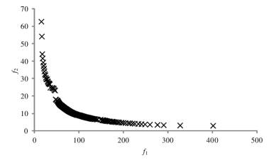
Figure 1: Input image $I_{1}$ used in experiments 1 and 2.

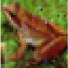
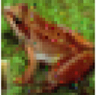
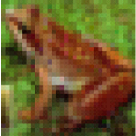
Figure 2: Results of experiment 1: obtained non-dominated soutions in $l_{0}$ versus $l_{1}$ norms scenario.

i) $f_{1}=18$	ii) $f_{1}=100$	iii) $f_{1}=327$
(a) Generated adversarial examlpes.
i) $f_{1}=18$	ii) $f_{1}=100$	iii) $f_{1}=327$
(b) Perturbed patterns.

Figure 3: Results of experiment 1: generated adversarial examples in $l_{0}$ versus $l_{1}$ norm scenario.

In this first experiment, the proposed method was applied to design adversarial examples for image $\mbox{\boldmath$I$}_{1}$ shown in Fig. 3 under $l_{0}$ versus $l_{1}$ norms scenario. That is, the first objective function was the number of perturbed pixels and the second objective function was the strength of changing pixel intensity on the perturbed pattern $\rho$. A constraint in which $P(\mathcal{C}(\mbox{\boldmath$I$}_{1}+\rho)=\mathcal{C}(\mbox{\boldmath$I$}_{1}))$ should be less than 0.2 was also considered. The proposed method uses the direct method and set $N_{w}=1$. Because the input image size was $32\times 32$ and they have 3 color channels, the total number of design variables was 3,072. The population size and the generation limit were set to 500 and 1,000, respectively.

In this experiment, the initial population was generated by dividing individuals into eight groups and imposing upper limits on the number of pixels to be changed and pixel perturbation ranges. Different upper limits were set for each group, 0.5%, 5%, 20%, 35%, 50%, 65%, 80%, and 95%, respectively, while pixel perturbation range were also limited to $\pm 200$, $\pm 200$, $\pm 100$, $\pm 50$, $\pm 33$, $\pm 25$, $\pm 20$, and $\pm 16$, respectively. The first two groups were also imposed to alter pixel values at least $\pm 150$ and $\pm 100$, respectively.

Fig. 3 shows the obtained non-dominated solutions, which demonstrates that the proposed method could generate various adversarial examples including ones in which 15 to over 400 pixels were changed and located between AEs generated by the previous EC- and gradient-based methods. Fig. 3(a) shows some examples of the obtained by the proposed method. All the three images shown in Fig. 3(a) were classified to ’deer’ with the confidence of 50.3%, 45.9%, and 41.8%, respectively whereas originally, $I_{1}$ was classified to ’frog’ with the confidence of 99.28%. Fig. 3(b) shows the perturbation patterns in which gray pixel indicates that were not modified, brighter pixels represent that were changed to their intensity was increased, and darker pixels represent that were changed in the opposite direction. From the perturbation patterns shown in Fig. 3(b), different perturbation patterns could be seen, though similar distributions were observed between ii) and iii).

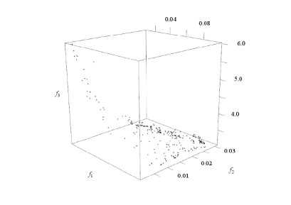
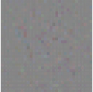
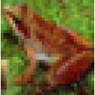
Figure 4: Results of experiment 2: obtained non-dominated solutions for generating adversarial example robust against rotation.

(a) Perturbation pattern $\rho$	(b) Perturbed image $\mbox{\boldmath$I_{1}$}+\mbox{\boldmath$\rho$}$

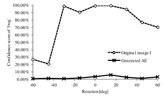
Figure 5: Results of experiment 2: generated adversarial example robust against rotation.

Figure 6: Results of experiment 2: robustness of the generated example against rotation.

TABLE I: Results of experiment 2: classification results and confidence of the generated example robust against rotation.

Rotation	Recognition results and confidence
angle	Clean image $I$				Perturbed image $I+\rho$
-60 deg	Frog:	26.8%	(Cat:	51.6%)	Frog:	1.0%	(Cat:	65.1%)
-45 deg	Frog:	20.9%	(Cat:	69.0%)	Frog:	1.2%	(Cat:	69.3%)
-30 deg	Frog:	98.9%			Frog:	0.9%	(Truck:	96.3%)
-15 deg	Frog:	90.6%			Frog:	1.8%	(Bird:	65.6%)
0 deg	Frog:	99.3%			Frog:	3.6%	(Deer:	77.0%)
15 deg	Frog:	99.5%			Frog:	5.9%	(Truck:	44.0%)
30 deg	Frog:	94.6%			Frog:	2.7%	(Truck:	64.5%)
45 deg	Frog:	77.0%			Frog:	1.1%	(Cat:	60.6%)
60 deg	Frog:	70.5%			Frog:	3.2%	(Cat:	47.6%)

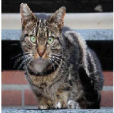
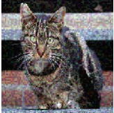
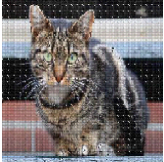
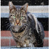
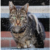
(a) Original (clean) image $I_{2}$	(b) Perturbed image $\mbox{\boldmath$I_{2}$}+\mbox{\boldmath$\rho$}$ by direct method	(c) Perturbed image $\mbox{\boldmath$I_{2}$}+\mbox{\boldmath$\rho$}$ by DCT-based method ($N_{AP}=1$)	(d) Perturbed image $\mbox{\boldmath$I_{2}$}+\mbox{\boldmath$\rho$}$ by DCT-based method ($N_{AP}=5$)	(e) Perturbed image $\mbox{\boldmath$I_{2}$}+\mbox{\boldmath$\rho$}$ by DCT-based method ($N_{AP}=10$)

Figure 7: Results of experiment 3: generated adversarial examples by direct and DCT-based methods.

TABLE II: Results of experiment 3: classification results and confidence of the generated example for VGG16.

			Perturbed images $I+\rho$
Rank	Clean image $I$		Direct method		DCT-based method
					$N_{AP}=1$		$N_{AP}=5$		$N_{AP}=10$
1st	Tabby:	60.8%	Envelope:	13.6%	jigsaw_puzzle:	76.4%	Purse:	20.8%	Coyote:	35.2%
2nd	Tiger_cat:	30.4%	Jigsaw_puzzle:	10.0%	tabby:	4.6%	Wood_rabbit:	13.2%	Wallaby:	16.0%
3rd	Egyptian_cat:	7.4%	Carton:	9.7%	tiger_cat:	2.8%	Jigsaw_puzzle:	7.0%	Wombat:	13.1%
4th	Doormat:	0.4%	Wallet:	9.7%	screen:	1.2%	Window_screen:	6.9%	Hare:	4.5%
5th	Radiator:	0.2%	Door_mat:	9.2%	prayer_rug:	1.1%	Mitten:	6.9%	German_shepherd	4.5%

TABLE III: Class labels regarded as correct ones in experiment 4.

Image	Original label	Labels regarded as correct
$I_{3}$	Airliner	Plane, Airship, Wing, Warplane, space_shuttle
$I_{4}$	tiger_cat	tabby, Egyptioan_cat, Lynx, Persian_cat, Siamese_cat
$I_{5}$	electric_guitar	acoustic_guitar, Violin, Banjo, cello
$I_{6}$	Plastic_bag	mailbag, sleeping_bag
$I_{7}$	Promontory	Seashore, Lakeside, Cliff, cliff_dwelling, Valley, Breakwater

IV-C Experiment 2: generating robust AEs against image transformation

In this experiment, taking the advantage of multi-objective optimization, we attempt to design robust adversarial examples against image transformation. Simple image rotation was considered as image transformation in this experiment because rotation has a greater influence than translation. Here, for the purpose of enhancing the robustness against image rotation, three objective functions were minimized: expected value and standard deviation of recognition accuracy of transformed images ($f_{1}(\cdot)$ and $f_{2}(\cdot)$), and $l_{1}$ norm of perturbation pattern $\rho$ ($f_{3}(\cdot)$). Two constraints were also imposed: the recognition accuracy of the target image was less than 10% without rotation, and the expected accuracy was less than 50%. The maximum rotation angle was set to $\pm 60$ degrees. The population size and the generation limit were set to 500 and 2,000, respectively. Other experimental conditions were the same as experiment 1.

Fig. 6 shows the obtained non-dominated solutions in the final generation. We picked up one non-dominated solution from them and Fig. 6 and Fig. 6 and show its image perturbation pattern and its robustness against rotation, respectively. The recognized class labels while changing rotation angle are shown in Table II. These results indicate that the generated AE successfully deceives the classifier in both with or without rotation cases.

IV-D Expleriment 3: effectiveness of the DCT-based method

In order to verify the effectiveness of the DCT-based method in higher resolution images, the direcet and DCT-based methods were compared on generating AE for an image in ImageNet-1000 under accuracy versus perturbation amount scenario. The first objective function is the classification accuracy to the original class. In this experiment we consider more general class than the original label assigned in ImageNet-1000, e.g., in the case generating AEs for image $\mbox{\boldmath$I$}_{2}$ shown in Fig. 7(a) which has a correct label ‘tabby’, labels of ‘Egyptian_cat’, ‘lynx’, ‘Persian_cat’, ‘Siamese_cat’, and ‘tiger_cat’ were also considered as correct labels. The second objective function is Root Mean Square Error (RMSE) between an original and perturbed images. A constraint, $P(\mathcal{C}(\mbox{\boldmath$I$}+\mbox{\boldmath$\rho$}))\leq 0.4$, was also considered to enhance search exploitation. In experiment 3 and subsequent experiments, we use the pretrained VGG16 as the target classifier.

In the case using the direct method, the total number of design variables was 5,625 because we changed the input image resolution to $224\times 224$, we set $N_{w}=3$, and the perturbation was added to brightness component of $I$. The DCT-based method requires less variables than the direct method, i.e., $848$, $1,104$, and $1,424$ dimensions for $N_{AP}=1$, $5$, and $10$, respectively.

Fig. 7 shows the representative AEs generated by the two methods, and Table II shows the recognition results and confidence scores of the generated AEs. Both methods could generate AEs that make the classifier misclassify. In addition, the DCT-based method generated AEs including less conspicuous patterns when $N_{AP}=10$.

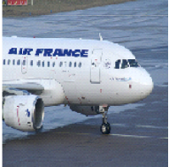
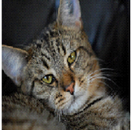
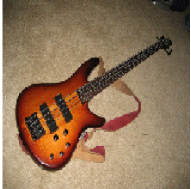
$I_{3}$	$I_{4}$	$I_{5}$	$I_{6}$	$I_{7}$
(a) Input clean images.
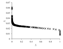
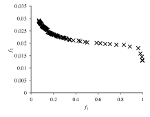
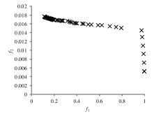
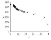
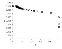
$I_{3}$	$I_{4}$	$I_{5}$	$I_{6}$	$I_{7}$
(b) Obtained non-dominated solutions.
$I_{3}$	$I_{4}$	$I_{5}$	$I_{6}$	$I_{7}$
(c) Designed perturbation pattern examples.
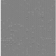
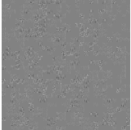
$I_{3}$	$I_{4}$	$I_{5}$	$I_{6}$	$I_{7}$
(d) Generated adversarial example images.

Figure 8: Results of experiment 4: input images, obtained non-dominated solutions, designed perturb patterns, and generated adversarial example images.

TABLE IV: Results of experiment 4: classification results and their confidence scores of original clean and perturbed images.

(a) $I_{3}$

Rank	Recognition results and confidence
	$\mathcal{C}(I_{3})$		$\mathcal{C}(I_{3}+\rho)$
1st	Airliner:	99.7%	aircraft_carrer:	94.9%
2nd	Wing:	2.6%	airliner:	3.0 %
3rd	Warplane:	0.0%	warplane:	1.4 %
4th	Space_shuttle:	0.0%	wing:	0.2%
5th	Airship:	0.0%	airship:	0.1%

(b) $I_{4}$

Rank	Recognition results and confidence
	$\mathcal{C}(I_{4})$		$\mathcal{C}(I_{4}+\rho)$
1st	tiger_cat:	81.9%	Leopard:	31.3%
2nd	tabby:	15.8%	jaguar:	10.5%
3rd	Egyptian_cat:	2.0%	lion:	9.3%
4th	Lynx:	0.2%	snow_leopard:	9.2%
5th	Lens_cap:	0.0%	cheetah:	9.1%

(c) $I_{5}$

Rank	Recognition results and confidence
	$\mathcal{C}(I_{5})$		$\mathcal{C}(I_{5}+\rho)$
1st	electric_guitar:	96.7%	Eft:	19.7%
2nd	acoustic_guitar:	2.7%	Banded_gecko:	11.3%
3rd	Violin:	0.3%	European_fire_salamander:	10.2%
4th	Banjo:	0.1%	Common_newt:	10.3%
5th	chello:	0.0%	alligator_lizard:	9.7%

(d) $I_{6}$

Rank	Recognition results and confidence
	$\mathcal{C}(I_{6})$		$\mathcal{C}(I_{6}+\rho)$
1st	Plastic_bag:	96.2%	sock:	22.5%
2nd	brassiere:	1.0%	brassiere:	8.6%
3rd	Toilet_tissue:	0.2%	pillow:	7.8%
4th	diaper:	0.2%	diaper:	7.8%
5th	sulphur-crested_cockatoo:	0.2%	handkerchief:	7.8%

(e) $I_{7}$

Rank	Recognition results and confidence
	$\mathcal{C}(I_{7})$		$\mathcal{C}(I_{7}+\rho)$
1st	Promontory:	96.6%	alp:	17.8%
2nd	seashore:	1.7%	Irish_wolfhound:	8.8%
3rd	cliff: :	1.4%	marmot:	7.5%
4th	bacon:	0.2%	timber_wolf:	7.4%
5th	lakeside:	0.0%	bighorn:	7.4%

IV-E Experiment 4: Other examples by DCT-based methods

In the final experiment, we attempted to generate AEs using the proposed DCT-based method for other images of ImageNet-1000 under the accuracy versus perturbation amount scenario. In this experiment, we added a solution candidate $\mbox{\boldmath$x$}_{\it 0}$ whose all variables were set to 0 into an initial population. Other experimental conditions were the same as those in experiment 3. Fig. 8(a) shows target original images whose resolution was changed to $224\times 224$. As in experiment 3, class labels similar to the original ones were regarded as correct ones, as shown in Table III.

Fig. 8(b) shows the distributions of obtained non-dominated solutions. Adding $\mbox{\boldmath$x$}_{\it 0}$ allowed the proposed method to clarify the trade-off relationship between the accuracy and the perturbation amount. Note that RMSE of $\mbox{\boldmath$x$}_{\it 0}$ was not zero because of the effect of DCT and inverse DCT process.

Fig.8 (c) and (d) shows examples of generated AEs and their perturbation patterns, respectively. Different types of perturbed patterns could be seen; AEs for $I_{4}$ and $I_{5}$ include small numbers of bright pixels, whereas AEs for $I_{3}$, $I_{6}$, and $I_{7}$ include striped and thin striped patterns. This demonstrates that the proposed method could adaptively generate AEs according to the target clean image properties.

Table IV shows the recognized classes and corresponding confidence scores. Here we focus on the results in each image. Because $I_{3}$ is an image of the front part of an airplane which involves less textures, there are very few classes that can induce misrecognition, resulting in erroneous recognition on label ’aircraft_carrier’. Other images $I_{4}$ through $I_{7}$ were the objects involving high frequency components and characteristic colors compared to $I_{3}$ and $I_{6}$, then their AEs made the classifier misclassified to various classes. Interestingly, $I_{5}$ and $I_{7}$ were erroneously recognized as various animals, whereas $I_{6}$ was misclassified mainly as artificial things.

IV-F Discussion

Although some of the above experiments involve high dimensional problems whose number of design variable exceeds 1,000, the proposed method could successfully generated AEs under black-box condition, i.e., without gradient information and other internal information of target classifiers except final recognition result (a class label and its confidence score). The above results revealed that the potential of EMO to AE design, though there is no guarantee that the obtained solutions were globally optima. It is possible that an AE design problem involves a highly multimodal fitness landscape including many promising quasi-optimal solutions, which EMO is appropriate for finding.

V Conclusions

This paper proposes an evolutionary multi-objective optimization approach to design adversarial examples that cannot be correctly recognized by machine learning models. The proposed method is black-box method that does not require internal information in the target models, and produces various AEs by simultaneously optimizing multiple objective functions that have trade-off relationship. Experimental resultse showed the potentials of the proposed EMO-based approach; e.g., the proposed method could produce various AEs that have different properties from ones generated by the previous EC- and gradient-based methods, and AEs robust against image rotation. This paper also demonstrated that the DCT-based method could generate AEs for higher resolution images.

On the other hand, the proposed method has many rooms for improvement from the viewpoint of comprehensively generating more diverse solutions. Introducing schemes to promote search exploration and to reduce problem dimension, and hybridization with local search are our important future work. The flexibility of EMO for designing objective functions would allow emerging new techniques to design AEs.

References

- [1] A. Krizhevsky, I. Sutskever, and G. E. Hinton, “Imagenet classification with deep convolutional neural networks,” in Advances in neural information processing systems, 2012, pp. 1097–1105.
- [2] I. Goodfellow, J. Pouget-Abadie, M. Mirza, B. Xu, D. Warde-Farley, S. Ozair, A. Courville, and Y. Bengio, “Generative adversarial nets,” in Advances in neural information processing systems, 2014, pp. 2672–2680.
- [3] P.-Y. Chen, H. Zhang, Y. Sharma, J. Yi, and C.-J. Hsieh, “Zoo: Zeroth order optimization based black-box attacks to deep neural networks without training substitute models,” in AISec@CCS, 2017.
- [4] A. Ilyas, L. Engstrom, A. Athalye, and J. Lin, “Black-box adversarial attacks with limited queries and information,” arXiv preprint arXiv:1804.08598, 2018.
- [5] N. Narodytska and S. P. Kasiviswanathan, “Simple black-box adversarial attacks on deep neural networks.” in CVPR Workshops, vol. 2, 2017.
- [6] N. Papernot, P. McDaniel, I. Goodfellow, S. Jha, Z. B. Celik, and A. Swami, “Practical black-box attacks against machine learning,” in Proceedings of the 2017 ACM on Asia Conference on Computer and Communications Security, 2017, pp. 506–519.
- [7] J. Su, D. V. Vargas, and K. Sakurai, “One pixel attack for fooling deep neural networks,” CoRR, vol. abs/1710.08864, 2017. [Online]. Available: http://arxiv.org/abs/1710.08864
- [8] A. Athalye, N. Carlini, and D. Wagner, “Obfuscated gradients give a false sense of security: Circumventing defenses to adversarial examples,” arXiv preprint arXiv:1802.00420, 2018.
- [9] D. Song, K. Eykholt, I. Evtimov, E. Fernandes, B. Li, A. Rahmati, F. Tramer, A. Prakash, and T. Kohno, “Physical adversarial examples for object detectors,” in 12th USENIX Workshop on Offensive Technologies (WOOT 18), 2018.
- [10] S.-M. Moosavi-Dezfooli, A. Fawzi, O. Fawzi, and P. Frossard, “Universal adversarial perturbations,” in 2017 IEEE Conference on Computer Vision and Pattern Recognition (CVPR), 2017, pp. 86–94.
- [11] C. Guo, J. R. Gardner, Y. You, A. G. Wilson, and K. Q. Weinberger, “Simple black-box adversarial attacks,” 2019. [Online]. Available: https://openreview.net/forum?id=rJeZS3RcYm
- [12] R. Shin and D. Song, “Jpeg-resistant adversarial images,” in NIPS 2017 Workshop on Machine Learning and Computer Security, 2017.
- [13] R. Storn and K. Price, “Differential evolution a simple and efficient heuristic for global optimization over continuous spaces,” J. of Global Optimization, vol. 11, pp. 341–359, 1997. [Online]. Available: http://dl.acm.org/citation.cfm?id=596061.596146
- [14] K. R. Rao and P. Yip, Discrete Cosine Transform: Algorithms, Advantages, Applications. San Diego, CA, USA: Academic Press Professional, Inc., 1990.
- [15] K. Shimoyama, A. Oyama, and K. Fujii, “Multi-objective six sigma approach applied to robust airfoil design for mars airplane,” in 48th AIAA/ASME/ASCE/AHS/ASC Structures, Structural Dynamics, and Materials Conference, 2007, p. 1966.
- [16] S. Ono and S. Nakayama, “Multi-objective particle swarm optimization for robust optimization and its hybridization with gradient search,” in Evolutionary Computation, 2009. CEC’09. IEEE Congress on. IEEE, 2009, pp. 1629–1636.
- [17] K. Deb, A. Pratap, S. Agarwal, and T. Meyarivan, “A fast and elitist multiobjective genetic algorithm: Nsga-ii,” Evolutionary Computation, IEEE Transactions on, vol. 6, no. 2, pp. 182–197, 2002.
- [18] Q. Zhang and H. Li, “MOEA/D: A Multiobjective Evolutionary Algorithm Based on Decomposition,” IEEE Transactions on Evolutionary Computation, vol. 11, no. 6, pp. 712–731, December 2007.
- [19] K. Deb and M. Goyal, “A combined genetic adaptive search (geneas) for engineering design,” Computer Science and Informatics, vol. 26, pp. 30–45, 1996.
- [20] D. P. Kingma and J. Ba, “Adam: A method for stochastic optimization,” arXiv preprint arXiv:1412.6980, 2014.
- [21] K. Simonyan and A. Zisserman, “Very deep convolutional networks for large-scale image recognition,” arXiv preprint arXiv:1409.1556, 2014.