Caching at Base Stations with Multi-Cluster Multicast Wireless Backhaul via Accelerated First-Order Algorithm

Abstract

Cloud radio access network (C-RAN) has been recognized as a promising architecture for next-generation wireless systems to support the rapidly increasing demand for higher data rate. However, the performance of C-RAN is limited by the backhaul capacities, especially for the wireless deployment. While C-RAN with fixed BS caching has been demonstrated to reduce backhaul consumption, it is more challenging to further optimize the cache allocation at BSs with multi-cluster multicast backhaul, where the inter-cluster interference induces additional non-convexity to the cache optimization problem. Despite the challenges, we propose an accelerated first-order algorithm, which achieves much higher content downloading sum-rate than a second-order algorithm running for the same amount of time. Simulation results demonstrate that, by simultaneously delivering the required contents to different multicast clusters, the proposed algorithm achieves significantly higher downloading sum-rate than those of time-division single-cluster transmission schemes. Moreover, it is found that the proposed algorithm allocates larger cache sizes to the farther BSs within the nearer clusters, which provides insight to the superiority of the proposed cache allocation.

I Introduction

To meet the dramatically increasing demand for higher data rate, cloud radio access network (C-RAN), where the base stations (BSs) are connected to a computation center via high-speed backhaul links for multi-BS cooperation, is a promising architecture for next-generation wireless systems [1, 2, 3]. However, the performance of C-RAN is mainly limited by the backhaul capacities from the computation center to the BSs, especially for the small-cell deployment, where high-speed optical fiber connections may not be available [4], and wireless backhaul is the only option.

On the other hand, with modern wireless data traffic being more and more dominated by videos and other multimedia data, content-centric communications exploiting multicast transmission and BS caching draw a lot of attention lately [5, 6, 7]. As multiple BSs in the same cluster share the same users’ data for BS cooperation, by multicasting users’ messages from the computation center to these BSs simultaneously, the broadcast nature of the wireless backhaul channels can be efficiently exploited. Furthermore, by proactively caching a fraction of popular contents at each BS, the amount of data to be delivered through the wireless backhaul is reduced, thus improving the system efficiency in terms of content downloading rate [8].

While C-RAN with BS caching has been investigated in [9, 10, 11, 12], they all assume fixed cache allocation among BSs and focus on how BS caching helps to improve the system performance. In particular, [9, 10, 11] investigate how BS caching facilitates the reduction of backhaul burden and power consumption. In [12], data-sharing and compression are combined to examine how BS caching help in improving the spectral efficiency. On the other hand, although cache optimization has been studied in [13, 14, 15, 16, 17], they only focus on the layer between the BS and the users, without considering the limitation of the backhaul efficiency. To the best of our knowledge, only the pioneering work [8] investigates cache optimization at BSs aiming at improving the backhaul efficiency between the computation center and the BSs.

Unfortunately, since [8] only considered a simplified C-RAN setup with a single cluster of BSs, the resulting caching scheme could not directly generalize to the more practical scenario with multiple BS clusters. For the multi-cluster scenario, the computation center is required to transmit different multicast data to different BS clusters simultaneously, resulting in inter-cluster interference, which in turn induces additional non-convexity to the cache optimization problem.

Despite the challenges mentioned above, this paper optimizes the cache allocation at BSs for a C-RAN with multi-cluster multicast backhaul, aiming to maximize the content downloading sum-rate of the wireless backhaul under a total cache budget constraint. Since cache placement impacts a much larger timescale than that of channel variations [18, 19, 4], the cache allocation should be optimized based on a large number of potential channel realizations. Furthermore, to maximize the content downloading sum-rate, various channel realizations requires tailored optimal beamformers, which are coupled in the optimization of cache sizes. Consequently, with a large number of beamfomers being nuisance variables, the cache allocation is a large-scale nonsmooth nonconvex problem. To solve this problem, we first tackle the non-smoothness and non-convexity by introducing auxiliary variables and constructing a sequence of quadratic convex functions in the successive convex approximation (SCA) framework. But instead of directly solving each convexified problem with the interior-point method, we further construct a strongly convex upper bound of the cost function, so that an accelerated first-order algorithm can be developed for solving each SCA subproblem in its dual domain.

Simulation results show that the proposed accelerated first-order algorithm achieves much higher content downloading sum-rate than a second-order algorithm running for the same amount of time. Moreover, by simultaneously delivering the required contents to different multicast clusters, the proposed algorithm achieves significantly higher downloading sum-rate than those of time-division single-cluster transmission schemes. Finally, it is found that the proposed algorithm proactively allocates larger cache sizes to the farther BSs within the nearer clusters, which provides insight to the superiority of the proposed cache allocation.

The remainder of this paper is organized as follows. System model and problem formulation are introduced in Section II. In Section III, an accelerated first-order algorithm is proposed for the cache allocation. The multi-cluster multicast beamforming (MCMB) design for content delivery is presented in Section IV. Simulation results and discussions are provided in Section V. Section VI concludes the paper.

Throughout this paper, scalars, vectors, and matrices are denoted by lower-case letters (e.g., $a$), lowercase bold letters (e.g., $\mathbf{a}$), and upper bold letters (e.g., $\mathbf{A}$), respectively. The complex domain is denoted by $\mathbb{C}$. We denote the transpose and conjugate transpose of a vector/matrix by $(\cdot)^{T}$ and $(\cdot)^{H}$, respectively. The real part, trace, and Frobenius-norm of a matrix are denoted by $\Re(\cdot)$, $\mathrm{Tr}(\cdot)$, and $\|\cdot\|_{F}$, respectively. The expectation of a random variable is denoted by $\mathbb{E}[\cdot]$, and the complex Gaussian distribution is represented as $\mathcal{CN}\left(\cdot,\cdot\right)$.

II System Model and Problem Formulation

Consider a downlink C-RAN with $G$ clusters of BSs connected to a computation center through wireless backhaul. To effectively utilize the wireless medium, the computation center adopts multicast beamforming to deliver users’ intended messages to each cluster, and the BSs in each cluster serve their users through cooperative transmission with data sharing [20, 21]. Furthermore, to alleviate the backhaul burden, each BS is equipped with a local cache to pre-store a subset of popular files. An example of such a cache enabled downlink C-RAN is illustrated in Fig. 1, where the BSs are clustered into $G$ disjoint clusters [22, 23]. In this paper, we assume that the BSs have been clustered, and focus on how to optimally allocate the cache sizes among the BSs to improve the backhaul efficiency.

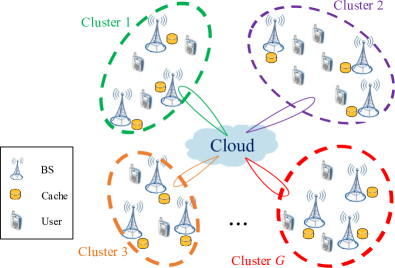
Figure 1: A downlink C-RAN consists of $G$ clusters of BSs, where each BS is equipped with a local cache.

Let $M$ and $N$ ($M>N$) denote the numbers of antennas at the computation center and each BS, respectively. Then the maximum number of independent data streams of each cluster is $d=\min\{M,N\}=N$, and the multicast beamforming matrix from the computation centre to the $g$-th cluster of BSs is denoted as $\mathbf{V}_{g}\in\mathbb{C}^{M\times d}$. Denoting the total number of BSs as $K$, we can express the received signal at the $k$-th BS as

$$\mathbf{y}_{k}=\underbrace{\mathbf{H}_{k}\mathbf{V}_{g_{k}}\mathbf{x}_{g_{k}}}_{\text{desired multicast signal}}+\underbrace{\sum_{g^{\prime}\neq g_{k}}\mathbf{H}_{k}\mathbf{V}_{g^{\prime}}\mathbf{x}_{g^{\prime}}}_{\text{inter-cluster interference}}+\mathbf{n}_{k},$$ (1)

where $\mathbf{H}_{k}\in\mathbb{C}^{N\times M}$ is the channel matrix from the computation centre to BS $k$, $g_{k}\in\{1,2,\ldots,G\}$ is the index of the group to which BS $k$ belongs, $\mathbf{x}_{g_{k}}\in\mathbb{C}^{d\times 1}$ is the data vector sent to cluster $g_{k}$, and $\mathbf{n}_{k}\sim\mathcal{CN}\left(\mathbf{0},\sigma_{k}^{2}\mathbf{I}_{N}\right)$ is the additive white Gaussian noise. Based on (1), the mutual information between the transmit signal $\mathbf{V}_{g_{k}}\mathbf{x}_{g_{k}}$ and the received signal $\mathbf{y}_{k}$ can be written as

$$I\left(\mathbf{V}_{g_{k}}\mathbf{x}_{g_{k}};\mathbf{y}_{k}\right)=\log\det\left(\mathbf{I}_{N}+\mathbf{H}_{k}\mathbf{V}_{g_{k}}\mathbf{V}_{g_{k}}^{H}\mathbf{H}_{k}^{H}\mathbf{J}_{k}\right),$$ (2)

where $\mathbf{J}_{k}\triangleq\left(\sum_{g^{\prime}\neq g_{k}}\mathbf{H}_{k}\mathbf{V}_{g^{\prime}}\mathbf{V}_{g^{\prime}}^{H}\mathbf{H}_{k}^{H}+\sigma_{k}^{2}\mathbf{I}_{N}\right)^{-1}$.

A central issue in C-RAN is to alleviate the backhaul burden during the peak traffic time [21]. To address this issue, caching highly popular files at BSs during off-peak hours provides a viable solution [10][24]. However, the network operator has a fixed budget to deploy only a limited amount of total cache size. Due to the limited cache size, each BS pre-stores fractions of popular contents during off-peak hours, and requests the rest from the computation center via wireless backhaul [8][25]. Specifically, BS $k$ caches the first $C_{k}$ bits of the file requested by cluster $g_{k}$. Denote $F_{g_{k}}$ as the total size of the file requested by cluster $g_{k}$, then BS $k$ requires to receive the rest $F_{g_{k}}-C_{k}$ bits of the file from the computation center when the file is delivered to mobile users [8][25]. With the knowledge of cached content at the BSs, an efficient joint cache-channel coding strategy [25] results in the content downloading rate of cluster $g$ as $R_{g}=\min_{k\in\mathcal{K}_{g}}\left\{\frac{I\left(\mathbf{V}_{g}\mathbf{x}_{g};\mathbf{y}_{k}\right)}{1-C_{k}/F_{g}}\right\}$ [8], where $\mathcal{K}_{g}$ denotes the set of BSs in cluster $g$. By substituting the mutual information $I\left(\mathbf{V}_{g}\mathbf{x}_{g};\mathbf{y}_{k}\right)$ into $R_{g}$, the downloading sum-rate of all the $G$ clusters of BSs can be written as

$$R_{\text{sum}} = \sum_{g=1}^{G}\min_{k\in\mathcal{K}_{g}}\Bigg{\{}\frac{F_{g}}{F_{g}-C_{k}}$$ (3)

$$\cdot\log\det\left(\mathbf{I}_{N}+\mathbf{H}_{k}\mathbf{V}_{g}\mathbf{V}_{g}^{H}\mathbf{H}_{k}^{H}\mathbf{J}_{k}\right)\Bigg{\}}.~{}~{}~{}~{}~{}$$

To improve the backhaul efficiency, the cache sizes $\left\{C_{k}\right\}$ should be allocated to maximize the content downloading sum-rate in (3). However, since cache placement happens in a much larger timescale than scheduling and transmission [14, 26, 27], cache sizes optimization should be based on long-term channel statistics. Furthermore, to maximize the content downloading sum-rate, the cache sizes should also be optimized together with the optimal beamformers. This gives the following cache size allocation problem:

$$\max_{\left\{C_{k}\right\}} \mathbb{E}_{\left\{\mathbf{H}_{k}\right\}}\Bigg{[}\max_{\left\{\mathbf{V}_{g}\right\}}\sum_{g=1}^{G}\min_{k\in\mathcal{K}_{g}}\Bigg{\{}\frac{F_{g}}{F_{g}-C_{k}}$$ (4a)

$$\cdot\log\det\left(\mathbf{I}_{N}+\mathbf{H}_{k}\mathbf{V}_{g}\mathbf{V}_{g}^{H}\mathbf{H}_{k}^{H}\mathbf{J}_{k}\right)\Bigg{\}}\Bigg{]},~{}~{}~{}~{}~{}$$

$$\text{s.t.}\ \sum_{g=1}^{G}\mathrm{Tr}\left(\mathbf{V}_{g}\mathbf{V}_{g}^{H}\right)\leq P_{\text{tot}},$$ (4b)

$$~{}~{}~{}~{}\ \sum_{k=1}^{K}C_{k}\leq C_{\text{tot}},$$ (4c)

$$~{}~{}~{}~{}\ 0\leq C_{k}\leq F_{g_{k}},~{}~{}\forall k=1,2,\ldots,K,$$ (4d)

where $P_{\text{tot}}$ is the total budget of the transmit power at the computation center, and $C_{\text{tot}}$ is the total budget of the cache size for the whole network. A common approach to tackle the expectation in (4a) is the sample approximation [28], which reformulates (4) as

$$\max_{\left\{C_{k}\right\},\left\{\mathbf{V}_{g,t}\right\}} \sum_{t=1}^{T}\sum_{g=1}^{G}\min_{k\in\mathcal{K}_{g}}\Bigg{\{}\frac{F_{g}}{F_{g}-C_{k}}\log\det\Big{(}\mathbf{I}_{N}$$ (5a)

$$+\mathbf{H}_{k,t}\mathbf{V}_{g,t}\mathbf{V}_{g,t}^{H}\mathbf{H}_{k,t}^{H}\mathbf{J}_{k,t}\Big{)}\Bigg{\}},~{}~{}~{}~{}~{}~{}$$

$$\text{s.t.}\ \sum_{g=1}^{G}\mathrm{Tr}\left(\mathbf{V}_{g,t}\mathbf{V}_{g,t}^{H}\right)\leq P_{\text{tot}},~{}~{}\forall t=1,2,\ldots,T,$$ (5b)

$$~{}~{}~{}~{}\ \sum_{k=1}^{K}C_{k}\leq C_{\text{tot}},$$ (5c)

$$~{}~{}~{}~{}\ 0\leq C_{k}\leq F_{g_{k}},~{}~{}\forall k=1,2,\ldots,K,$$ (5d)

where $T$ is the sample size, $\left\{\mathbf{H}_{k,t}\right\}_{k=1}^{K}$ are the $t$-th channel samples, which can be drawn from any given channel distribution or historical channel realizations, $\left\{\mathbf{V}_{g,t}\right\}_{g=1}^{G}$ are the corresponding beamformers, and $\mathbf{J}_{k,t}\triangleq\left(\sum_{g^{\prime}\neq g_{k}}\mathbf{H}_{k,t}\mathbf{V}_{g^{\prime},t}\mathbf{V}_{g^{\prime},t}^{H}\mathbf{H}_{k,t}^{H}+\sigma_{k}^{2}\mathbf{I}_{N}\right)^{-1}$.

However, problem (5) is challenging to solve due to three reasons. Firstly, the objective function (5a) is nonsmooth since the content downloading rate of each BS cluster is the minimum over $\left|\mathcal{K}_{g}\right|$ terms. Secondly, the objective function (5a) is also nonconcave due to the nonconcave coupling between $\frac{F_{g}}{F_{g}-C_{k}}$ and $\log\det\left(\mathbf{I}_{N}+\mathbf{H}_{k,t}\mathbf{V}_{g,t}\mathbf{V}_{g,t}^{H}\mathbf{H}_{k,t}^{H}\mathbf{J}_{k,t}\right)$, and the involvement of $\left\{\mathbf{V}_{g,t}\right\}$ in the inter-cluster interference inside the expression of $\mathbf{J}_{k,t}$. Thirdly, since the sample size $T$ is generally large for good approximation, problem (5) is imposed by a large number of variables and constraints, which induces a heavy computational burden.

Remark 1: For multicast transmission, the file requests in the same multicast group should arrive within a very short time period. Although this assumption is a little strong for mobile users, it makes more sense for the considered scenario in this paper, where the multicast receivers are BSs that require data sharing for coordinated multipoint joint processing rather than mobile users. Therefore, it is reasonable to assume that the BSs in the same cluster request the content simultaneously.

Remark 2: If the computation center transmits data to each BS directly, it either transmits the data in a time-division fashion, or transmits multiple beams at the same time. For using the time division transmission, it avoids interference among beams, but it would take a long time to transmit, as one BS is served after another. On the other hand, if multiple beams are transmitted at the same time, the transmission time is shortened, but the interference among beams would cause severe decoding error.

Remark 3: Strictly speaking, $C_{k}$ is a discrete variable, which makes the optimization problem (5) combinatorial and highly complex. To make it more tractable, as in the most relevant work [8], we set $C_{k}$ as a continuous variable. Consequently, it is much easier to reveal the insight of caching as shown in Section VI. For practical implementation of the scheme, the solution of $C_{k}$ can be rounded off to the nearest integer after the continuous optimization problem is solved.

III Accelerated First-Order Algorithm for Cache Allocation

In this section, we strive to solve the large-scale nonsmooth nonconvex cache size allocation problem (5). Specifically, we first tackle the non-smoothness and non-convexity of problem (5) by introducing auxiliary variables and constructing a sequence of quadratic convex functions in the SCA framework. Then, instead of directly solving each convexified problem with the interior-point method, we further construct a strongly convex upper bound of the cost function, so that an accelerated first-order algorithm is developed for solving each SCA subproblem in its dual domain.

III-A Tackling Non-Smoothness and Non-Convexity

We first tackle the non-smoothness of the objective function (5a). Since (5a) is the minimum over $\left|\mathcal{K}_{g}\right|$ terms, by introducing a set of auxiliary variables $\left\{\eta_{g,t}\right\}$ such that $\eta_{g,t}\leq\frac{1}{F_{g}-C_{k}}\log\det\left(\mathbf{I}_{N}+\mathbf{H}_{k,t}\mathbf{V}_{g,t}\mathbf{V}_{g,t}^{H}\mathbf{H}_{k,t}^{H}\mathbf{J}_{k,t}\right)$, $\forall k\in\mathcal{K}_{g}$, problem (5) can be equivalently transformed into the following smooth problem:

$$\min_{\left\{C_{k}\right\},\left\{\mathbf{V}_{g,t},\eta_{g,t}\right\}}-\sum_{t=1}^{T}\sum_{g=1}^{G}F_{g}\eta_{g,t},$$ (6a)

$$\text{s.t.}\ \sum_{g=1}^{G}\mathrm{Tr}\left(\mathbf{V}_{g,t}\mathbf{V}_{g,t}^{H}\right)\leq P_{\text{tot}},~{}~{}\forall t=1,2,\ldots,T,$$ (6b)

$$~{}~{}~{}~{}\ \sum_{k=1}^{K}C_{k}\leq C_{\text{tot}},$$ (6c)

$$~{}~{}~{}~{}\ 0\leq C_{k}\leq F_{g_{k}},~{}~{}\forall k=1,2,\ldots,K,$$ (6d)

$$~{}~{}~{}~{}\ (F_{g_{k}}-C_{k})\eta_{g_{k},t}-\log\det\Big{(}\mathbf{I}_{N}+\mathbf{H}_{k,t}\mathbf{V}_{g_{k},t}\mathbf{V}_{g_{k},t}^{H}$$

$$\cdot\mathbf{H}_{k,t}^{H}\mathbf{J}_{k,t}\Big{)}\leq 0,\forall k=1,2,\ldots,K,\forall t=1,2,\ldots,T.$$ (6e)

However, due to the nonconvex coupling between $C_{k}$ and $\eta_{g_{k},t}$, and the involvement of $\left\{\mathbf{V}_{g,t}\right\}$ in the inter-cluster interference inside the expression of $\mathbf{J}_{k,t}$, the constraint (6) is nonconvex, making problem (6) still challenging to solve. For the special case of $G=1$, $\mathbf{J}_{k}$ would reduce to $1/\sigma_{k}^{2}\mathbf{I}_{N}$, which is independent of the variable $\mathbf{V}_{1}$. Therefore, by introducing an auxiliary variable $\mathbf{W}_{1}=\mathbf{V}_{1}\mathbf{V}_{1}^{H}$ and dropping the rank constraint of $\mathbf{W}_{1}$ [8], (6) would be convex over $\mathbf{W}_{1}$. However, for the general case of $G>1$, since $\mathbf{J}_{k}$ involves variables $\left\{\mathbf{V}_{g}\right\}$, the above convexity over $\left\{\mathbf{W}_{g}\right\}$ does not hold. Thus, for the general setting of $G>1$, the non-convexity of (6) is difficult to tackle.

A prevalent technique to tackle nonconvex constraints is the successive convex approximation (SCA) [29], in which nonconvex constraints are approximated by a sequence of convex constraints. When the nonconvex constraints are in difference of convex (DC) forms, a common approach for convex approximation is the convex-concave procedure (CCP) [30]. Nevertheless, CCP is not applicable to (6), since it is not in a DC form. To address this issue, we construct a sequence of convex constraints to approximate (6) by quadratically convexifying the left-hand-side of (6). Specifically, given any fixed $C_{k}^{(i)}$, $\eta_{g_{k},t}^{(i)}$, and $\left\{\mathbf{V}_{g,t}^{(i)}\right\}_{g=1}^{G}$, we define a convex quadratic function

$$f_{k,t}^{(i)}\left(C_{k},\eta_{g_{k},t},\left\{\mathbf{V}_{g,t}\right\}_{g=1}^{G}\right)\triangleq\sum_{g=1}^{G}\mathrm{Tr}\left(\mathbf{V}_{g,t}^{H}\mathbf{A}_{k,t}^{(i)}\mathbf{V}_{g,t}\right)$$

$$+2\Re\left\{\mathrm{Tr}\left(\mathbf{B}_{k,t}^{(i)}\mathbf{V}_{g_{k},t}\right)\right\}+\frac{\eta_{g_{k},t}^{2}+C_{k}^{2}}{2}+F_{g_{k}}\eta_{g_{k},t}$$

$$-\left(\eta_{g_{k},t}^{(i)}+C_{k}^{(i)}\right)\left(\eta_{g_{k},t}+C_{k}\right)+b_{k,t}^{(i)},$$ (7)

where $\mathbf{A}_{k,t}^{(i)}$, $\mathbf{B}_{k,t}^{(i)}$, and $b_{k,t}^{(i)}$ are given by

$$\mathbf{A}_{k,t}^{(i)} \triangleq \mathbf{H}_{k,t}^{H}\mathbf{U}_{k,t}^{(i)}\left(\mathbf{I}_{d}-\left(\mathbf{U}_{k,t}^{(i)}\right)^{H}\mathbf{H}_{k,t}\mathbf{V}_{g_{k},t}^{(i)}\right)^{-1}$$ (8)

$$\cdot\left(\mathbf{U}_{k,t}^{(i)}\right)^{H}\mathbf{H}_{k,t},$$

$$\mathbf{B}_{k,t}^{(i)} \triangleq -\left(\mathbf{I}_{d}-\left(\mathbf{U}_{k,t}^{(i)}\right)^{H}\mathbf{H}_{k,t}\mathbf{V}_{g_{k},t}^{(i)}\right)^{-1}$$ (9)

$$\cdot\left(\mathbf{U}_{k,t}^{(i)}\right)^{H}\mathbf{H}_{k,t},$$

$$b_{k,t}^{(i)} \triangleq \mathrm{Tr}\Bigg{(}\left(\mathbf{I}_{d}-\left(\mathbf{U}_{k,t}^{(i)}\right)^{H}\mathbf{H}_{k,t}\mathbf{V}_{g_{k},t}^{(i)}\right)^{-1}$$ (10)

$$\cdot\left(\mathbf{I}_{d}+\sigma_{k}^{2}\left(\mathbf{U}_{k,t}^{(i)}\right)^{H}\mathbf{U}_{k,t}^{(i)}\right)\Bigg{)}$$

$$+\log\det\left(\mathbf{I}_{d}-\left(\mathbf{U}_{k,t}^{(i)}\right)^{H}\mathbf{H}_{k,t}\mathbf{V}_{g_{k},t}^{(i)}\right)$$

$$+\frac{\left(\eta_{g_{k},t}^{(i)}+C_{k}^{(i)}\right)^{2}}{2}-d,$$

with

$$\mathbf{U}_{k,t}^{(i)} \triangleq \left(\sum_{g=1}^{G}\mathbf{H}_{k,t}\mathbf{V}_{g,t}^{(i)}\left(\mathbf{V}_{g,t}^{(i)}\right)^{H}\mathbf{H}_{k,t}^{H}+\sigma_{k}^{2}\mathbf{I}_{N}\right)^{-1}$$ (11)

$$\cdot\mathbf{H}_{k,t}\mathbf{V}_{g_{k},t}^{(i)}.$$

Then, we can establish two properties of $f_{k,t}^{(i)}\left(C_{k},\eta_{g_{k},t},\left\{\mathbf{V}_{g,t}\right\}_{g=1}^{G}\right)$ with the following proposition.

Proposition 1.

The defined function $f_{k,t}^{(i)}\left(C_{k},\eta_{g_{k},t},\left\{\mathbf{V}_{g,t}\right\}_{g=1}^{G}\right)$ in (4) satisfies:

(1.1) $f_{k,t}^{(i)}\left(C_{k},\eta_{g_{k},t},\left\{\mathbf{V}_{g,t}\right\}_{g=1}^{G}\right)\geq(F_{g_{k}}-C_{k})\eta_{g_{k},t}-\log\det\left(\mathbf{I}_{N}+\mathbf{H}_{k,t}\mathbf{V}_{g_{k},t}\mathbf{V}_{g_{k},t}^{H}\mathbf{H}_{k,t}^{H}\mathbf{J}_{k,t}\right)$, where the equality holds at $C_{k}=C_{k}^{(i)}$, $\eta_{g_{k}}=\eta_{g_{k}}^{(i)}$, and $\mathbf{V}_{g,t}=\mathbf{V}_{g,t}^{(i)}$, $\forall g=1,2,\ldots,G$.

(1.2) $\frac{\partial}{\partial\tau}f_{k,t}^{(i)}\left(C_{k}^{(i)},\eta_{g_{k},t}^{(i)},\left\{\mathbf{V}_{g,t}^{(i)}\right\}_{g=1}^{G}\right)=\frac{\partial}{\partial\tau}\Bigg{(}(F_{g_{k}}-C_{k}^{(i)})\eta_{g_{k},t}^{(i)}-\log\det\Bigg{(}\mathbf{I}_{N}+\mathbf{H}_{k,t}\mathbf{V}_{g_{k},t}^{(i)}\left(\mathbf{V}_{g_{k},t}^{(i)}\right)^{H}$ $\mathbf{H}_{k,t}^{H}\mathbf{J}_{k,t}^{(i)}\Bigg{)}\Bigg{)}$, where $\tau$ represents $C_{k}$, $\eta_{g_{k}}$, or any element of $\mathbf{V}_{g,t}$, $\forall g=1,2,\ldots,G$, and $\mathbf{J}_{k,t}^{(i)}=\left.\mathbf{J}_{k,t}\right|_{\big{\{}\mathbf{V}_{g,t}\big{\}}_{g=1}^{G}=\big{\{}\mathbf{V}_{g,t}^{(i)}\big{\}}_{g=1}^{G}}$.

Proof: See Appendix A.   

In particular, property (1.1) means that the left-hand-sides of the original nonconvex constraints are upper bounded by the left-hand-sides of the constructed convex constraints; while property (1.2) means that the gradients of the left-hand-sides of both the constructed convex constraints and the original nonconvex constraints are equal at the expansion points. Based on the two properties in Proposition 1, the left-hand-side of the nonconvex constraint (6) is upper bounded by $f_{k,t}^{(i)}\left(C_{k},\eta_{g_{k},t},\left\{\mathbf{V}_{g,t}\right\}_{g=1}^{G}\right)$, and hence (6) can be successively approximated by

$$f_{k,t}^{(i)}\left(C_{k},\eta_{g_{k},t},\left\{\mathbf{V}_{g,t}\right\}_{g=1}^{G}\right)\leq 0,$$

$$~{}~{}\forall k=1,2,\ldots,K,~{}~{}\forall t=1,2,\ldots,T,$$ (12)

which is convex since $f_{k,t}^{(i)}\left(C_{k},\eta_{g_{k},t},\left\{\mathbf{V}_{g,t}\right\}_{g=1}^{G}\right)$ is convex quadratic. With the sequence of convex constraints constructed in (III-A), problem (6) can be iteratively solved in the SCA framework, with the $i$-th SCA subproblem written as

$$\left[\left\{C_{k}^{(i+1)}\right\},\left\{\mathbf{V}_{g,t}^{(i+1)},\eta_{g,t}^{(i+1)}\right\}\right]$$ (13a)

$$= \arg\min_{\left\{C_{k}\right\},\left\{\mathbf{V}_{g,t},\eta_{g,t}\right\}}-\sum_{t=1}^{T}\sum_{g=1}^{G}F_{g}\eta_{g,t},$$

$$\text{s.t.}\ \sum_{g=1}^{G}\mathrm{Tr}\left(\mathbf{V}_{g,t}\mathbf{V}_{g,t}^{H}\right)\leq P_{\text{tot}},~{}~{}\forall t=1,2,\ldots,T,$$ (13b)

$$~{}~{}~{}~{}\ \sum_{k=1}^{K}C_{k}\leq C_{\text{tot}},$$ (13c)

$$~{}~{}~{}~{}\ 0\leq C_{k}\leq F_{g_{k}},~{}~{}\forall k=1,2,\ldots,K,$$ (13d)

$$~{}~{}~{}~{}\ f_{k,t}^{(i)}\left(C_{k},\eta_{g_{k},t},\left\{\mathbf{V}_{g,t}\right\}_{g=1}^{G}\right)\leq 0,$$

$$~{}~{}\forall k=1,2,\ldots,K,~{}~{}\forall t=1,2,\ldots,T.$$ (13e)

III-B First-Order Algorithm in Dual Domain

While problem (13) can be optimally solved with the interior point method, due to the large number of variables and constraints (induced by the large sample size $T$), such a method would incur a heavy computational cost. To avoid such a heavy computational burden, we strive to develop a first-order algorithm, which alternatively performs a gradient step and a projection step. However, since problem (13) is imposed by coupling constraints (13b), (13c), and (13), the projection onto (13b)-(13) would be highly complicated.

To address this issue, we develop another form of the $i$-th SCA subproblem of (6) by majorizing the cost function (6a) with a strongly convex upper bound. Specifically, given any fixed $\left\{C_{k}^{(i)}\right\}$ and $\left\{\mathbf{V}_{g,t}^{(i)},\eta_{g,t}^{(i)}\right\}$, the cost function (6a) can be strongly convexified by adding three positive quadratic terms:

$$\Upsilon^{(i)}\left(\left\{C_{k}\right\},\left\{\mathbf{V}_{g,t},\eta_{g,t}\right\}\right)$$ (14)

$$= -\sum_{t=1}^{T}\sum_{g=1}^{G}F_{g}\eta_{g,t}+\frac{\rho_{1}}{2}\sum_{t=1}^{T}\sum_{g=1}^{G}\left(\eta_{g,t}-\eta_{g,t}^{(i)}\right)^{2}$$

$$+\rho_{2}\sum_{t=1}^{T}\sum_{g=1}^{G}\left\|\mathbf{V}_{g,t}-\mathbf{V}_{g,t}^{(i)}\right\|_{F}^{2}$$

$$+\frac{\rho_{3}}{2}\sum_{k=1}^{K}\left(C_{k}-C_{k}^{(i)}\right)^{2},$$

where $\rho_{1}$, $\rho_{2}$, and $\rho_{3}$ are fixed positive parameters. Consequently, (14) serves as a tight upper bound of (6a), with their function values equal at $\left\{C_{k}\right\}=\left\{C_{k}^{(i)}\right\}$ and $\left\{\mathbf{V}_{g,t},\eta_{g,t}\right\}=\left\{\mathbf{V}_{g,t}^{(i)},\eta_{g,t}^{(i)}\right\}$. Following the same procedure for convexifying the constraints of (6) in the last section, another valid $i$-th SCA subproblem of (6) can be written as

$$\left[\left\{C_{k}^{(i+1)}\right\},\left\{\mathbf{V}_{g,t}^{(i+1)},\eta_{g,t}^{(i+1)}\right\}\right]$$

$$= \arg\min_{\left\{C_{k}\right\},\left\{\mathbf{V}_{g,t},\eta_{g,t}\right\}}\Upsilon^{(i)}\left(\left\{C_{k}\right\},\left\{\mathbf{V}_{g,t},\eta_{g,t}\right\}\right),$$

$$\text{s.t.}~{}~{}\eqref{Cache3 power},\eqref{Cache3 cache1},\eqref{Cache3 cache2},\eqref{Cache3 rate}.$$

Based on the strong convexity of $\Upsilon^{(i)}\left(\left\{C_{k}\right\},\left\{\mathbf{V}_{g,t},\eta_{g,t}\right\}\right)$, we can derive the dual problem of (III-B) in closed-form with the following proposition.

Proposition 2.

The dual problem of (III-B) is

$$\max_{\left\{\delta_{t}\right\},\left\{\lambda_{k,t}\right\},\mu} \Upsilon^{(i)}\left(\left\{C_{k}^{\diamond}\right\},\left\{\mathbf{V}_{g,t}^{\diamond},\eta_{g,t}^{\diamond}\right\}\right)$$ (16a)

$$+\sum_{t=1}^{T}\delta_{t}\left(\sum_{g=1}^{G}\mathrm{Tr}\left(\mathbf{V}_{g,t}^{\diamond}\left(\mathbf{V}_{g,t}^{\diamond}\right)^{H}\right)-P_{\text{tot}}\right)$$

$$+\sum_{t=1}^{T}\sum_{k=1}^{K}\lambda_{k,t}f_{k,t}^{(i)}\left(C_{k}^{\diamond},\eta_{g_{k},t}^{\diamond},\left\{\mathbf{V}_{g,t}^{\diamond}\right\}_{g=1}^{G}\right)$$

$$+\mu\left(\sum_{k=1}^{K}C_{k}^{\diamond}-C_{\text{tot}}\right),$$

$$\text{s.t.}\ \mu\geq 0,~{}~{}\delta_{t}\geq 0,~{}~{}\lambda_{k,t}\geq 0,$$

$$~{}~{}\forall k=1,2,\ldots,K,~{}~{}\forall t=1,2,\ldots,T,$$ (16b)

where $\left\{\mathbf{V}_{g,t}^{\diamond},\eta_{g,t}^{\diamond}\right\}$ and $\left\{C_{k}^{\diamond}\right\}$ are uniquely given in the following closed forms:

$$\eta_{g,t}^{\diamond}=\eta_{g,t}^{(i)}+\frac{\left(1-\sum_{k\in\mathcal{K}_{g}}\lambda_{k,t}\right)F_{g}+\sum_{k\in\mathcal{K}_{g}}\lambda_{k,t}C_{k}^{(i)}}{\rho_{1}+\sum_{k\in\mathcal{K}_{g}}\lambda_{k,t}},$$

$$~{}~{}\forall g=1,2,\ldots,G,~{}~{}\forall t=1,2,\ldots,T,$$ (17)

$$\mathbf{V}_{g,t}^{\diamond} = \left(\left(\rho_{2}+\delta_{t}\right)\mathbf{I}_{M}+\sum_{k=1}^{K}\lambda_{k,t}\mathbf{A}_{k,t}^{(i)}\right)^{-1}$$ (18)

$$\cdot\left(\rho_{2}\mathbf{V}_{g,t}^{(i)}-\sum_{k\in\mathcal{K}_{g}}\lambda_{k,t}\left(\mathbf{B}_{k,t}^{(i)}\right)^{H}\right),$$

$$\forall g=1,2,\ldots,G,~{}~{}\forall t=1,2,\ldots,T,$$

$$C_{k}^{\diamond}=\min\Bigg{\{}\max\Bigg{\{}\Bigg{(}C_{k}^{(i)}+$$

$$\frac{\sum_{t=1}^{T}\lambda_{k,t}\eta_{g_{k},t}^{(i)}-\mu}{\rho_{3}+\sum_{t=1}^{T}\lambda_{k,t}}\Bigg{)},0\Bigg{\}},F_{g_{k}}\Bigg{\}},\forall k=1,2,\ldots,K.~{}~{}~{}~{}~{}$$ (19)

Proof: See Appendix B.   

Denoting the the dual objective function in (16a) as $D\left(\left\{\delta_{t}\right\},\left\{\lambda_{k,t}\right\},\mu\right)$, and noticing that the values of $\left\{\mathbf{V}_{g,t}^{\diamond},\eta_{g,t}^{\diamond}\right\}$ and $\left\{C_{k}^{\diamond}\right\}$ are uniquely determined by (2)-(2), we can obtain the partial derivatives as

$$\begin{cases}\frac{\partial D}{\partial\delta_{t}}=\sum_{g=1}^{G}\mathrm{Tr}\left(\mathbf{V}^{\diamond}_{g,t}\left(\mathbf{V}^{\diamond}_{g,t}\right)^{H}\right)-P_{\text{tot}},\cr\frac{\partial D}{\partial\lambda_{k,t}}=f_{k,t}^{(i)}\left(C_{k}^{\diamond},\eta_{g_{k},t}^{\diamond},\left\{\mathbf{V}_{g,t}^{\diamond}\right\}_{g=1}^{G}\right),\cr\frac{\partial D}{\partial\mu}=\sum_{k=1}^{K}C_{k}^{\diamond}-C_{\text{tot}},\end{cases}$$ (20)

thus the projected gradient step increasing $D\left(\left\{\delta_{t}\right\},\left\{\lambda_{k,t}\right\},\mu\right)$ can be expressed as

$$\begin{cases}\left(\delta_{t}+\beta_{s}\left(\sum_{g=1}^{G}\mathrm{Tr}\left(\mathbf{V}^{\diamond}_{g,t}\left(\mathbf{V}^{\diamond}_{g,t}\right)^{H}\right)-P_{\text{tot}}\right)\right)^{+},\cr\left(\lambda_{k,t}+\beta_{s}f_{k,t}^{(i)}\left(C_{k}^{\diamond},\eta_{g_{k},t}^{\diamond},\left\{\mathbf{V}_{g,t}^{\diamond}\right\}_{g=1}^{G}\right)\right)^{+},\cr\left(\mu+\beta_{s}\left(\sum_{k=1}^{K}C_{k}^{\diamond}-C_{\text{tot}}\right)\right)^{+},\end{cases}$$ (21)

where $\beta_{s}$ is the step size at the $s$-th iteration, and $(\cdot)^{+}\triangleq\max(\cdot,0)$ is the non-negativity projection over (16).

Algorithm 1 First-Order Algorithm for Solving (III-B)

1:Compute $\mathbf{A}_{k,t}^{(i)}$, $\mathbf{B}_{k,t}^{(i)}$, and $b_{k,t}^{(i)}$ with (8)-(10), $\forall k=1,2,\ldots,K,~{}~{}\forall t=1,2,\ldots,T.$

2:Initialize $\delta_{t}=1$, $\forall t=1,2,\ldots,T$; $\lambda_{k,t}=1$, $\forall k=1,2,\ldots,K$, $\forall t=1,2,\ldots,T$; $\mu=1$.

3:repeat ($s=1,2,\ldots$)

4:Update $\left\{\mathbf{V}^{\diamond}_{g,t},\eta^{\diamond}_{g,t}\right\}$ and $\left\{C^{\diamond}_{k}\right\}$ with (2)-(2).

5:Update $\left\{\delta_{t}\right\}$, $\left\{\lambda_{k,t}\right\}$, and $\mu$ with (21).

6:until convergence

7:Output $\left\{\mathbf{V}^{(i+1)}_{g,t},\eta^{(i+1)}_{g,t}\right\}=\left\{\mathbf{V}^{\diamond}_{g,t},\eta^{\diamond}_{g,t}\right\}$ and $\left\{C^{(i+1)}_{k}\right\}=\left\{C^{\diamond}_{k}\right\}$.

By iteratively updating $\left\{\delta_{t}\right\}$, $\left\{\lambda_{k,t}\right\}$, and $\mu$ with (21), we can obtain the optimal solution to the dual problem (16). Correspondingly, the optimal $\left\{\mathbf{V}_{g,t},\eta_{g,t}\right\}$ and $\left\{C_{k}\right\}$ to the primal problem (III-B) is given by substituting the optimal $\left\{\delta_{t}\right\}$, $\left\{\lambda_{k,t}\right\}$, and $\mu$ into (2)-(2). We summarize this procedure for solving problem (III-B) in Algorithm 1, which is guaranteed to converge to the global optimum of (16) at a rate of $\mathcal{O}\left(1/s\right)$, if the step size $\beta_{s}$ is smaller than the inverse of the Lipschitz constant of $\nabla D$ [31]. Moreover, notice that the primal problem (III-B) is convex, thus the convergent optimum of (16) is also the global optimum of (III-B), provided that (III-B) is strictly feasible [32].

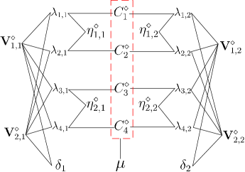
Figure 2: Parallel structure of Algorithm 1 when $T=2$, $G=2$, $K=4$, $\mathcal{K}_{1}=\left\{1,2\right\}$, and $\mathcal{K}_{2}=\left\{3,4\right\}$.

Notice that each iteration of Algorithm 1 can be executed in parallel. In particular, both the $2GT+K$ primal variables in line 4 and the $(K+1)T+1$ dual variables in line 5 can be updated in parallel. An example of the parallel structure of Algorithm 1 is shown in Fig. 2, where $T=2$, $G=2$, $K=4$, $\mathcal{K}_{1}=\left\{1,2\right\}$, and $\mathcal{K}_{2}=\left\{3,4\right\}$. The $12$ primal variables $\mathbf{V}^{\diamond}_{1,1}$, $\mathbf{V}^{\diamond}_{2,1}$, $\mathbf{V}^{\diamond}_{1,2}$, $\mathbf{V}^{\diamond}_{2,2}$, $\eta_{1,1}^{\diamond}$, $\eta_{2,1}^{\diamond}$, $\eta_{1,2}^{\diamond}$, $\eta_{2,2}^{\diamond}$, $C_{1}^{\diamond}$, $C_{2}^{\diamond}$, $C_{3}^{\diamond}$, and $C_{4}^{\diamond}$ can be simultaneously updated. Furthermore, the update of each primal variable only depends on a few dual variables (e.g., the update of $\eta_{1,1}^{\diamond}$ only depends on $\lambda_{1,1}$ and $\lambda_{2,1}$), thus the message passing overhead is small. Similarly, the dual variables can also be simultaneously updated and each depends on only a few primal variables. Due to this parallel structure, Algorithm 1 has the potential of leveraging the modern multi-core multi-thread processor architecture for speeding up the computation.

III-C Acceleration with Momentum Technique

Algorithm 2 Accelerated First-Order Algorithm for Solving (III-B)

1:Compute $\mathbf{A}_{k,t}^{(i)}$, $\mathbf{B}_{k,t}^{(i)}$, and $b_{k,t}^{(i)}$ with (8)-(10), $\forall k=1,2,\ldots,K,~{}~{}\forall t=1,2,\ldots,T.$

2:Initialize $\delta_{t}=1$, $\forall t=1,2,\ldots,T$; $\lambda_{k,t}=1$, $\forall k=1,2,\ldots,K$, $\forall t=1,2,\ldots,T$; $\mu=1$; $\theta^{(0)}=1.$

3:repeat ($s=1,2,\ldots$)

4:Update $\theta^{(s)}$ with (24).

5:Update $\left\{\mathbf{V}^{\diamond}_{g,t},\eta^{\diamond}_{g,t}\right\}$ and $\left\{C^{\diamond}_{k}\right\}$ with (2)-(2).

6:Update $\left\{\tilde{\delta}_{t}^{(s)}\right\}$, $\left\{\tilde{\lambda}_{k,t}^{(s)}\right\}$, and $\tilde{\mu}^{(s)}$ with (22).

7:Update $\left\{\delta_{t}\right\}$, $\left\{\lambda_{k,t}\right\}$, and $\mu$ with (23).

8:until convergence

9:Output $\left\{\mathbf{V}^{(i+1)}_{g,t},\eta^{(i+1)}_{g,t}\right\}=\left\{\mathbf{V}^{\diamond}_{g,t},\eta^{\diamond}_{g,t}\right\}$ and $\left\{C^{(i+1)}_{k}\right\}=\left\{C^{\diamond}_{k}\right\}$.

Although Algorithm 1 only involves the gradient information and can be executed in parallel, as a first-order algorithm, it may require a large number of iterations to converge. To improve the convergence speed, we further apply the momentum technique [33] to accelerate Algorithm 1. In particular, the projected gradient step in (21) is modified by updating $\tilde{\delta}_{t}^{(s)}$, $\tilde{\lambda}_{k,t}^{(s)}$, and $\tilde{\mu}^{(s)}$:

$$\begin{cases}\left(\delta_{t}+\beta_{s}\left(\sum_{g=1}^{G}\mathrm{Tr}\left(\mathbf{V}^{\diamond}_{g,t}\left(\mathbf{V}^{\diamond}_{g,t}\right)^{H}\right)-P_{\text{tot}}\right)\right)^{+},\cr\left(\lambda_{k,t}+\beta_{s}f_{k,t}^{(i)}\left(C_{k}^{\diamond},\eta_{g_{k},t}^{\diamond},\left\{\mathbf{V}_{g,t}^{\diamond}\right\}_{g=1}^{G}\right)\right)^{+},\cr\left(\mu+\beta_{s}\left(\sum_{k=1}^{K}C_{k}^{\diamond}-C_{\text{tot}}\right)\right)^{+},\end{cases}$$ (22)

$$\begin{cases}\delta_{t}\leftarrow\tilde{\delta}_{t}^{(s)}+\frac{\theta^{(s-1)}-1}{\theta^{(s)}}\left(\tilde{\delta}_{t}^{(s)}-\tilde{\delta}_{t}^{(s-1)}\right),\cr\lambda_{k,t}\leftarrow\tilde{\lambda}_{k,t}^{(s)}+\frac{\theta^{(s-1)}-1}{\theta^{(s)}}\left(\tilde{\lambda}_{k,t}^{(s)}-\tilde{\lambda}_{k,t}^{(s-1)}\right),\cr\mu\leftarrow\tilde{\mu}^{(s)}+\frac{\theta^{(s-1)}-1}{\theta^{(s)}}\left(\tilde{\mu}^{(s)}-\tilde{\mu}^{(s-1)}\right),\end{cases}$$ (23)

where $\theta^{(s)}$ is the weighting parameter to dynamically control the momentums $\tilde{\delta}_{t}^{(s)}-\tilde{\delta}_{t}^{(s-1)}$, $\tilde{\lambda}_{k,t}^{(s)}-\tilde{\lambda}_{k,t}^{(s-1)}$, and $\tilde{\mu}^{(s)}-\tilde{\mu}^{(s-1)}$. To achieve fast convergence, $\theta^{(s)}$ is updated by [33]

$$\theta^{(s)}=\frac{1+\sqrt{1+4\left(\theta^{(s-1)}\right)^{2}}}{2}.$$ (24)

By using (22)-(24), the accelerated first-order algorithm for solving problem (III-B) is summarized in Algorithm 2. The key insight of the acceleration lies in the momentums $\tilde{\delta}_{t}^{(s)}-\tilde{\delta}_{t}^{(s-1)}$, $\tilde{\lambda}_{k,t}^{(s)}-\tilde{\lambda}_{k,t}^{(s-1)}$, and $\tilde{\mu}^{(s)}-\tilde{\mu}^{(s-1)}$ in (23) (without these momentums, Algorithm 2 would reduce to Algorithm 1). These momentums utilize previous updates to generate an overshoot, so that the update using (22) and (23) in Algorithm 2 is more aggressive than the conventional gradient step (21) in Algorithm 1. On the other hand, to ensure these overshoots to be well behaved, the momentums are controlled by a sequence of weighting parameters $\left\{\theta^{(s)}\right\}$. With $\left\{\theta^{(s)}\right\}$ updated using (24), Algorithm 2 is guaranteed to converge to the the global optimum of (16) at a rate of $\mathcal{O}\left(1/s^{2}\right)$ [33].

III-D Overall Algorithm for Solving (5)

With the $i$-th SCA subproblem (III-B) solved by Algorithm 2, the overall algorithm for solving the cache size allocation problem (5) is summarized in Algorithm 3. Since the constructed convex constraint (III-A) satisfies properties (1.1) and (1.2) of Proposition 1, and the constructed upper bound $\Upsilon^{(i)}\left(\left\{C_{k}\right\},\left\{\mathbf{V}_{g,t},\eta_{g,t}\right\}\right)$ tightly approximates the cost function (6a), Algorithm 3 is guaranteed to converge to a stationary point of problem (6) [34], which is equivalent to problem (5).

Notice that Algorithm 3 is based on the SCA framework, thus it requires to be initialized from a feasible point. For simplicity, as shown in line 1, we provide a feasible initial point for Algorithm 3 by equally allocating the total transmit power $P_{\text{tot}}$ and the total cache sizes $C_{\text{tot}}$ to each $\mathbf{V}_{g,t}^{(0)}$ and $C_{k}^{(0)}$ respectively, and $\eta_{g,t}^{(0)}$ is obtained from (6) by substituting $\mathbf{V}_{g,t}=\mathbf{V}_{g,t}^{(0)}$ and $C_{k}=C_{k}^{(0)}$.

Algorithm 3 Overall Algorithm for Solving (5)

1:Initialization:

1. $\mathbf{V}_{g,t}^{(0)}=\sqrt{\frac{P_{\text{tot}}}{GMd}}\mathbf{1}_{M\times d},~{}~{}\forall g=1,2,\ldots,G,~{}~{}\forall t=1,2,\ldots,T$;

2. $C_{k}^{(0)}=C_{\text{tot}}/K,~{}~{}\forall k=1,2,\ldots,K$;

3. $\eta_{g,t}^{(0)}=\min_{k\in\mathcal{K}_{g}}\Big{\{}\frac{1}{F_{g}-C_{k}^{(0)}}\log\det\Big{(}\mathbf{I}_{N}+\mathbf{H}_{k,t}\mathbf{V}_{g,t}^{(0)}$ $\cdot\left(\mathbf{V}_{g,t}^{(0)}\right)^{H}\mathbf{H}_{k,t}^{H}\mathbf{J}_{k,t}^{(0)}\Big{)}\Big{\}},~{}~{}\forall g=1,2,\ldots,G,~{}~{}\forall t=1,2,\ldots,T$.

2:repeat ($i=0,1,\ldots$)

3:Solve the $i$-th SCA subproblem (III-B) with Algorithm 2.

4:until convergence

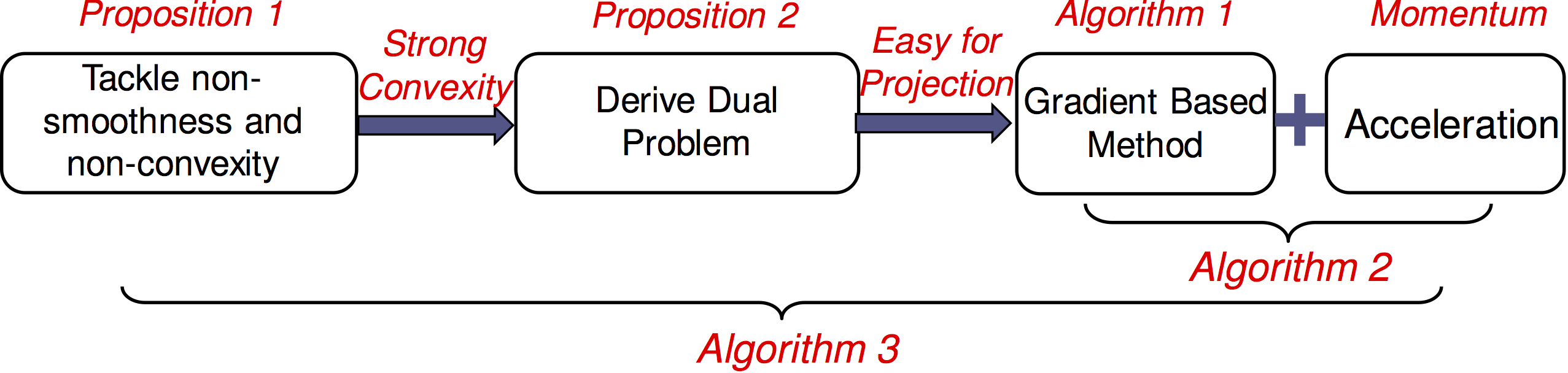
Figure 3: Proposed algorithm framework for the cache allocation problem (5).

In summary, the extension from the single-cluster scenario [8] to the more general multi-cluster scenario brings two new challenges. First, the inter-cluster interference induces non-convexity in the optimization problem. Although SCA provides a general framework to tackle the non-convexity, it is still challenging to convexify the nonconvex constraint (6), which is not in the common difference of convex form. To tackle this challenge, we establish Proposition 1, which tightly approximates (6) by quadratically convexifying its left-hand-side. Second, even after tackling the non-convexity, it is still challenging to solve the resulting SCA subproblem (13) due to its large numbers of coupling constraints, which make the first-order projected gradient descent method not applicable. To get around the coupling constraints, we further establish Proposition 2, which exploits the strong convexity of (14), so that the dual problem (16) can be efficiently solved by the proposed accelerated gradient based method. The overall framework for solving the cache allocation problem (5) is depicted in Fig. 3.

IV MCMB Design for Content Delivery

To evaluate the performance of the proposed cache size allocation in Section III, we further design the MCMB for content delivery with fixed $\left\{C_{k}\right\}$. Since only the multicast beamformers $\left\{\mathbf{V}_{g}\right\}$ are optimized for maximizing the instantaneous downloading sum-rate $R_{\text{sum}}$ in (3), the MCMB design problem becomes

$$\max_{\left\{\mathbf{V}_{g}\right\}}\sum_{g=1}^{G}\min_{k\in\mathcal{K}_{g}}\left\{\frac{F_{g}}{F_{g}-C_{k}}\log\det\left(\mathbf{I}_{N}+\mathbf{H}_{k}\mathbf{V}_{g}\mathbf{V}_{g}^{H}\mathbf{H}_{k}^{H}\mathbf{J}_{k}\right)\right\},$$ (25a)

$$\text{s.t.}\ \sum_{g=1}^{G}\mathrm{Tr}\left(\mathbf{V}_{g}\mathbf{V}_{g}^{H}\right)\leq P_{\text{tot}},$$ (25b)

which can be equivalently transformed into the following smooth problem:

$$\min_{\left\{\mathbf{V}_{g},\eta_{g}\right\}}-\sum_{g=1}^{G}F_{g}\eta_{g},$$ (26a)

$$\text{s.t.}\ \sum_{g=1}^{G}\mathrm{Tr}\left(\mathbf{V}_{g}\mathbf{V}_{g}^{H}\right)\leq P_{\text{tot}},$$ (26b)

$$(F_{g_{k}}-C_{k})\eta_{g_{k}}-\log\det\left(\mathbf{I}_{N}+\mathbf{H}_{k}\mathbf{V}_{g_{k}}\mathbf{V}_{g_{k}}^{H}\mathbf{H}_{k}^{H}\mathbf{J}_{k}\right)$$

$$\leq 0,\forall k=1,2,\ldots,K.$$ (26c)

Notice that problem (26) is a simplified version of (6) when $T=1$ and $\left\{C_{k}\right\}$ are fixed. Following similar derivations to that of the cache allocation problem in the last section (see Appendix C), the $i$-th SCA subproblem of (26) can be written as

$$\left\{\mathbf{V}_{g}^{(i+1)},\eta_{g}^{(i+1)}\right\}=\arg\min_{\left\{\mathbf{V}_{g},\eta_{g}\right\}}-\sum_{g=1}^{G}F_{g}\eta_{g},$$ (27a)

$$\text{s.t.}\ \sum_{g=1}^{G}\mathrm{Tr}\left(\mathbf{V}_{g}\mathbf{V}_{g}^{H}\right)\leq P_{\text{tot}}.$$ (27b)

$$~{}~{}~{}~{}\ (F_{g_{k}}-C_{k})\eta_{g_{k}}+h_{k}^{(i)}\left(\left\{\mathbf{V}_{g}\right\}\right)\leq 0,~{}~{}\forall k=1,2,\ldots,K,$$ (27c)

where $h_{k}^{(i)}\left(\left\{\mathbf{V}_{g}\right\}\right)$ is given in (C.1) of Appendix C. Since subproblem (27) is convex, it can be optimally solved by the standard optimization toolbox based on the interior-point method (e.g., CVX [35]). Notice that different from (13), the SCA subproblem (27) involves only a single channel realization, thus the interior-point method would not induce a heavy computational burden.

Algorithm 4 Proposed Algorithm for Solving (25)

1:Initialize $\mathbf{V}_{g}^{(0)}=\sqrt{\frac{P_{\text{tot}}}{GMd}}\mathbf{1}_{M\times d},~{}~{}\forall g=1,2,\ldots,G$.

2:repeat ($i=0,1,\ldots$)

3:Compute $\mathbf{\hat{A}}_{k}^{(i)}$, $\mathbf{\hat{B}}_{k}^{(i)}$, and $\hat{b}_{k}^{(i)}$ with (C.2)-(C.4), $\forall k=1,2,\ldots,K$.

4:Solve the $i$-th SCA subproblem (27) with CVX.

5:until convergence

The overall framework for solving the MCMB design problem (25) is depicted in Fig. 4, and the algorithm is summarized in Algorithm 4. Without loss of generality, the initialization of Algorithm 4 is obtained by equally allocating the total transmit power $P_{\text{tot}}$ to each $\mathbf{V}_{g}^{(0)}$. Since the constructed convex constraint in (C.6) satisfies properties C.a and C.b in Appendix C, Algorithm 4 is guaranteed to converge to a stationary point of problem (26) [34].

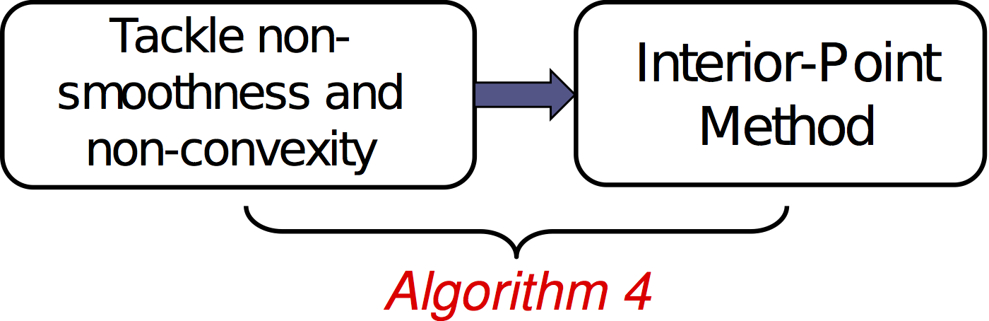
Figure 4: Proposed algorithm framework for the content delivery problem (25).

V Caching Multiple Files with Different Popularities

While the files were assumed to have the same popularity in Section III, it can be extended to the more general case with multiple files having different popularities. In particular, denote $f_{g}\in\mathcal{F}_{g}=\left\{c_{g,1},c_{g,2},\ldots,c_{g,\left|\mathcal{F}_{g}\right|}\right\}$ as a potential file to be requested by a BS group $g$ with the file’s request probability $p_{f_{g}}$ (with $\sum_{f_{g}\in\mathcal{F}_{g}}{p_{f_{g}}}=1$). Let $\mathbf{f}\triangleq\left[f_{1},f_{2},\ldots,f_{G}\right]^{H}$ and $\mathcal{F}\triangleq\mathcal{F}_{1}\times\mathcal{F}_{2}\times\ldots\times\mathcal{F}_{G}$, then the request probability of $\mathbf{f}$ is $p_{\mathbf{f}}=\prod_{g=1}^{G}p_{f_{g}}$ and we have $\sum_{\mathbf{f}\in\mathcal{F}}p_{\mathbf{f}}=1$. Each BS $k$ caches $C_{k,f_{g_{k}}}/F_{f_{g_{k}}}$ of the file $f_{g_{k}}$. Consequently, under the total cache size constraint $\sum_{k=1}^{K}\sum_{f_{g_{k}}\in\mathcal{F}_{g_{k}}}C_{k,f_{g_{k}}}\leq C_{\text{tot}}$, the cache size allocation problem with different popularities can be formulated as

$$\max_{\left\{C_{k,f_{g}}\right\},\left\{\mathbf{V}_{g,t,\mathbf{f}}\right\}}\sum_{t=1}^{T}\sum_{g=1}^{G}\sum_{\mathbf{f}\in\mathcal{F}}p_{\mathbf{f}}\min_{k\in\mathcal{K}_{g}}\Bigg{\{}\frac{F_{f_{g}}}{F_{f_{g}}-C_{k,f_{g}}}$$

$$\cdot\log\det\left(\mathbf{I}_{N}+\mathbf{H}_{k,t,\mathbf{f}}\mathbf{V}_{g,t,\mathbf{f}}\mathbf{V}_{g,t,\mathbf{f}}^{H}\mathbf{H}_{k,t,\mathbf{f}}^{H}\mathbf{J}_{k,t,\mathbf{f}}\right)\Bigg{\}},~{}~{}~{}~{}~{}$$ (28a)

$$\text{s.t.}\ \sum_{g=1}^{G}\mathrm{Tr}\left(\mathbf{V}_{g,t,\mathbf{f}}\mathbf{V}_{g,t,\mathbf{f}}^{H}\right)\leq P_{\text{tot}},~{}~{}\forall\mathbf{f}\in\mathcal{F},~{}~{}\forall t=1,2,\ldots,T,$$ (28b)

$$~{}~{}~{}~{}\ \sum_{k=1}^{K}\sum_{f_{g_{k}}\in\mathcal{F}_{g_{k}}}C_{k,f_{g_{k}}}\leq C_{\text{tot}},~{}~{}~{}~{}~{}~{}~{}~{}~{}~{}~{}~{}~{}~{}~{}~{}~{}~{}~{}~{}~{}~{}~{}~{}~{}~{}~{}~{}~{}~{}~{}~{}~{}~{}~{}~{}~{}~{}$$ (28c)

$$~{}~{}~{}~{}\ 0\leq C_{k,f_{g_{k}}}\leq F_{f_{g_{k}}},~{}~{}\forall f_{g_{k}}\in\mathcal{F}_{g_{k}},~{}~{}\forall k=1,2,\ldots,K,$$ (28d)

where $\left\{\mathbf{H}_{k,t,\mathbf{f}}\right\}_{k=1}^{K}$ and $\left\{\mathbf{V}_{g,t,\mathbf{f}}\right\}_{g=1}^{G}$ are the corresponding channel matrices and beamformers, respectively. Notice that when $p_{\mathbf{f}}$ with different $\mathbf{f}$ are equal, (28) will reduce to (5). With the only difference between (28) and (5) lying in the weighting parameter $p_{\mathbf{f}}$ in (28), (28) can be solved using the same algorithm framework as Algorithm 3 proposed in Section III. The corresponding algorithm is summarized as Algorithm 5 in Appendix D. Finally, notice that an unpopular file would lead to a small $C_{k,f_{g_{k}}}$. But no matter $C_{k,f_{g_{k}}}$ is big or small, for content delivery, as shown in Section IV, whenever a file (even an unpopular file) is requested by the BSs, the computation center must provide multicast transmission immediately. Therefore, there is no delay during the transmission.

VI Simulation Results and Discussions

In this section, we evaluate the performance of the proposed cache size allocation in terms of downloading sum-rate through simulations. All simulations are performed on MATLAB R2017b running on a Windows x64 machine with 3.3 GHz CPU and 8 GB RAM.

We consider a downlink C-RAN with $G=4$ clusters of BSs, where each cluster consists of $3$ BSs. In particular, the distances between the computation center and the BSs in the $4$ clusters are $\left\{160,260,360\right\}$, $\left\{200,280,360\right\}$, $\left\{160,280,400\right\}$, and $\left\{240,320,400\right\}$ in meters, respectively. The computation center is equipped with $M=20$ antennas and each BS is equipped with $N=2$ antennas. The path loss at distance $D$ kilometers follows $128.1+37.6\log_{10}(D)$ in dB, and the small-scale channel is subject to Rayleigh fading. We use $T=100$ sets of channel realizations for solving the cache allocation problem (5). The maximum transmit power at the computation center is $P_{\text{tot}}=40$ W and the antenna gain is $17$ dBi [8]. The backhaul channel bandwidth is $20$ MHz and the background noise power spectral density is $-150$ dBm/Hz. The content size is $F_{g}=100,\forall g=1,2,3,4$, and the budget of the total cache size is $C_{\text{tot}}=120$.

The step size $\beta_{s}$ in Algorithm 1 and Algorithm 2 is fixed as $1$, and the parameters in (14) are fixed as $\rho_{1}=10^{5}$, $\rho_{2}=10^{4}$, and $\rho_{3}=1$. The iterations of Algorithm 1, Algorithm 2, and Algorithm 4 terminate when the relative changes of the corresponding objective functions between two consecutive iterations are less than $10^{-3}$. The SCA iteration of Algorithm 3 stops when the relative decrease of the cost function (6a) in the last $100$ iterations is less than $10^{-2}$.

VI-A Convergence Behaviors of Proposed Algorithms

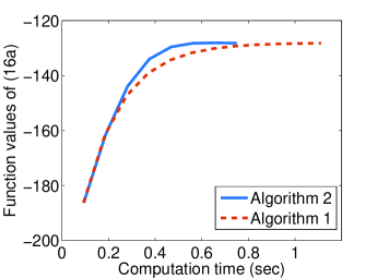
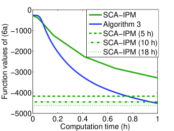
Figure 5: (a) Convergence behavior of the inner iteration of Algorithm 3. (b) Convergence behavior of the outer iteration of Algorithm 3.

First, we show the convergence behavior of Algorithm 3 for solving the cache size allocation problem (5). Since the inner iteration of Algorithm 3 is based on Algorithm 1 or Algorithm 2, we illustrate the convergence behaviors of Algorithm 1 and Algorithm 2 in Fig. 5. It can be seen that they both converge to the same objective function value, but Algorithm 2 achieves much faster convergence than Algorithm 1, with computation time roughly half of that of Algorithm 1. This demonstrates the effectiveness of the acceleration technique exploited in Algorithm 2. Therefore, we only adopt Algorithm 2 as the inner iteration of Algorithm 3 for the rest of simulations.

On the other hand, the convergence behavior of the outer iteration of Algorithm 3 is shown in Fig. 5. To show the complexity advantage of Algorithm 3, we compare it with a second-order algorithm (termed as SCA-IPM), which also applies the SCA framework but solves each SCA subproblem (13) with the interior-point method. It can be seen that with the proposed algorithm and SCA-IPM running for the same amount of time, the proposed algorithm achieves a much lower function value of (6a). Furthermore, in order to achieve the same accuracy, SCM-IPM requires 5 to 18 times more computation time. This demonstrates that Algorithm 3 is more suitable for the cache size allocation problem (5) with a large number of variables and constraints. Notice that the computation time is measured based on MATLAB implementation. In industrial implementation, more efficient programming languages (e.g., C++) would be adopted to achieve even more efficient execution.

VI-B Performance of Proposed Algorithms on Downloading Sum-Rate

In this subsection, we demonstrate the effectiveness of the proposed cache size allocation in terms of downloading sum-rate (with MCMB design using Algorithm 4). The sum-rate achieved by the proposed cache allocation is compared to that of the uniform cache size allocation. Furthermore, since the recent work [8] is designed for the single-cluster multicast scenario without inter-cluster interference, we compare with a benchmark by extending [8] to the multi-cluster multicast scenario in a time-division multiplexing manner. Specifically, for a $G$-cluster multicast scenario, to avoid the inter-cluster interference, each cluster utilizes $1/G$ of the total time resources. Consequently, without inter-cluster interference, the cache allocation problem can be directly solved by the proposed algorithm in [8]. To show the importance of modeling the inter-cluster interference, we also add a baseline, which directly applies [8] without modeling the interference for optimization.

Figure 6 illustrates the cumulative distribution functions of downloading sum-rates obtained by different schemes under $400$ channel realizations. It can be seen that, by simultaneously delivering the required contents to different multicast clusters, the multi-cluster transmission schemes achieve significantly higher downloading sum-rate than the time-division single-cluster transmission schemes. This demonstrates the necessity of the multi-cluster multicast transmission for improving the backhaul efficiency. Moreover, with the optimized cache size, the downloading sum-rate achieved by the proposed algorithm is much higher than that of the uniform caching scheme. On the other hand, without effective interference management, the direct application of [8] results in the lowest downloading sum-rate. This demonstrates the necessity of modeling the interference for the multi-cluster multicast scenario. The comparison among various schemes is summarized in Table I. It can be seen that the average downloading sum-rate achieved by the proposed approach is more than 2 times of that of the extension of [8], and more than 10 times of that of the direct application of [8], respectively.

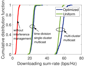
Figure 6: Cumulative distribution functions of downloading sum-rates obtained by different schemes under $400$ channel realizations.

TABLE I: Average downloading sum-rate comparison

Schemes	The way to handle multi-cluster interference	Average downloading sum-rate
Proposed approach	Multi-cluster beamforming	$59$ bps/Hz
Direct application of [8]	No mitigation	$5$ bps/Hz
Extending [8] to multi-cluster scenario	Time-division multiplexing	$26$ bps/Hz

To reveal the insight of the superiority of the proposed cache size allocation, we show the optimized cache sizes among different BSs in Fig. 7. It can be seen that, within a cluster, the cache size allocated by the proposed algorithm increases with the distance between the BS and the computation center. For instance, in Cluster 1, BS 3 is allocated with the largest cache sizes. On the other hand, among different clusters, the proposed algorithm allocates larger cache sizes to the nearer clusters. For example, Cluster 1 and Cluster 4 are allocated with the the largest and the smallest cache sizes, respectively.

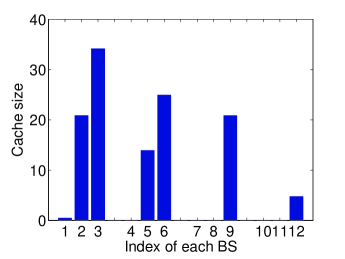
Figure 7: Cache size allocation results among different BSs. The distances between the computation center and the BSs in the $4$ clusters are $\left\{160,260,360\right\}$, $\left\{200,280,360\right\}$, $\left\{160,280,400\right\}$, and $\left\{240,320,400\right\}$ in meters.

Finally, to investigate the impact of file popularity, the allocated cache sizes among different files are shown in Fig. 8, where there are $2$ clusters of BSs, and each cluster consists of $3$ BSs situated in $160$, $260$, and $360$ meters from the computation center. In Fig. 8(a) to Fig. 8(c), each BS requests $2$ files with popularities $(p_{1}=0.5,p_{2}=0.5)$, $(p_{1}=0.7,p_{2}=0.3)$, and $(p_{1}=0.9,p_{2}=0.1)$, respectively. It can be seen that the weakest BS $3$ and BS $6$ are always allocated the largest cache sizes in all the three cases. Furthermore, as the difference between the popularities of the two files increases, the file with higher popularity is allocated much larger cache size. For instance, as shown in Fig. 8(c), when $p_{1}=0.9$ and $p_{2}=0.1$, the file with higher popularity is allocated almost all the cache.

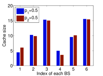
(a) $p_{1}=0.5,p_{2}=0.5$

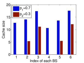
(b) $p_{1}=0.7,p_{2}=0.3$

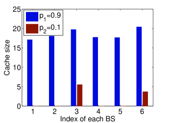
(c) $p_{1}=0.9,p_{2}=0.1$

Figure 8: Cache size allocation results among different files with different popularities.

VII Conclusions

Caching at BSs was studied for a C-RAN with multi-cluster multicast backhaul, with the aim of maximizing the content downloading sum-rate of the wireless backhaul under a total cache budget constraint. To solve this large-scale nonsmooth nonconvex problem, we proposed an accelerated first-order algorithm, which achieves much higher content downloading sum-rate than a second-order algorithm running for the same amount of time. Moreover, with multi-cluster multicast transmission, the proposed algorithm achieves significantly higher downloading sum-rate than those of time-division single-cluster transmission schemes. In addition, simulation results revealed that the proposed algorithm allocates larger cache sizes to farther BSs within nearer clusters, which provides insight to the superiority of the proposed cache allocation.

Appendix A Proof of Proposition 1

From (4), we can rewrite $f_{k,t}^{(i)}\left(C_{k},\eta_{g_{k},t},\left\{\mathbf{V}_{g,t}\right\}_{g=1}^{G}\right)=\phi_{k,t}^{(i)}\left(\left\{\mathbf{V}_{g,t}\right\}_{g=1}^{G}\right)+\psi_{k,t}^{(i)}\left(C_{k},\eta_{g_{k},t}\right)$, where

$$\phi_{k,t}^{(i)}\left(\left\{\mathbf{V}_{g,t}\right\}_{g=1}^{G}\right)=\sum_{g=1}^{G}\mathrm{Tr}\left(\mathbf{V}_{g,t}^{H}\mathbf{A}_{k,t}^{(i)}\mathbf{V}_{g,t}\right)$$

$$+2\Re\left\{\mathrm{Tr}\left(\mathbf{B}_{k,t}^{(i)}\mathbf{V}_{g_{k},t}\right)\right\}+b_{k,t}^{(i)}-\frac{\left(\eta_{g_{k},t}^{(i)}+C_{k}^{(i)}\right)^{2}}{2},~{}~{}~{}~{}~{}~{}$$ (A.1)

$$\psi_{k,t}^{(i)}\left(C_{k},\eta_{g_{k},t}\right)=\frac{\eta_{g_{k},t}^{2}+C_{k}^{2}}{2}-\left(\eta_{g_{k},t}^{(i)}+C_{k}^{(i)}\right)$$

$$\cdot\left(\eta_{g_{k},t}+C_{k}\right)+F_{g_{k}}\eta_{g_{k},t}+\frac{\left(\eta_{g_{k},t}^{(i)}+C_{k}^{(i)}\right)^{2}}{2}.$$ (A.2)

From (A), we have

$$\psi_{k,t}^{(i)}\left(C_{k},\eta_{g_{k},t}\right)-(F_{g_{k}}-C_{k})\eta_{g_{k},t}$$ (A.3)

$$= \frac{1}{2}\left(\eta_{g_{k},t}+C_{k}-\eta_{g_{k},t}^{(i)}-C_{k}^{(i)}\right)^{2}\geq 0,$$

where the equality holds at $C_{k}=C_{k}^{(i)}$ and $\eta_{g_{k}}=\eta_{g_{k}}^{(i)}$.

Next, we prove

$$\phi_{k,t}^{(i)}\left(\left\{\mathbf{V}_{g,t}\right\}_{g=1}^{G}\right)$$ (A.4)

$$\geq -\log\det\left(\mathbf{I}_{N}+\mathbf{H}_{k,t}\mathbf{V}_{g_{k},t}\mathbf{V}_{g_{k},t}^{H}\mathbf{H}_{k,t}^{H}\mathbf{J}_{k,t}\right).~{}~{}~{}~{}$$

More specifically, applying $\det\left(\mathbf{I}+\mathbf{X}\mathbf{Y}\right)=\det\left(\mathbf{I}+\mathbf{Y}\mathbf{X}\right)$, we have

$$\log\det\left(\mathbf{I}_{N}+\mathbf{H}_{k,t}\mathbf{V}_{g_{k},t}\mathbf{V}_{g_{k},t}^{H}\mathbf{H}_{k,t}^{H}\mathbf{J}_{k,t}\right)$$ (A.5)

$$= \log\det\left(\mathbf{I}_{d}+\mathbf{V}_{g_{k},t}^{H}\mathbf{H}_{k,t}^{H}\mathbf{J}_{k,t}\mathbf{H}_{k,t}\mathbf{V}_{g_{k},t}\right).$$

Applying the Woodbury matrix identity to the right-hand-side of (A.5), we have

$$\log\det\left(\mathbf{I}_{N}+\mathbf{H}_{k,t}\mathbf{V}_{g_{k},t}\mathbf{V}_{g_{k},t}^{H}\mathbf{H}_{k,t}^{H}\mathbf{J}_{k,t}\right)$$ (A.6)

$$= \log\det\left({\left(\underbrace{\mathbf{I}_{d}-\mathbf{U}_{k,t}^{H}\mathbf{H}_{k,t}\mathbf{V}_{g_{k},t}}_{\mathbf{Q}_{k,t}}\right)}^{-1}\right),$$

where $\mathbf{U}_{k,t}$ is defined as

$$\mathbf{U}_{k,t}\triangleq\left(\sum_{g=1}^{G}\mathbf{H}_{k,t}\mathbf{V}_{g,t}\mathbf{V}_{g,t}^{H}\mathbf{H}_{k,t}^{H}+\sigma_{k}^{2}\mathbf{I}_{N}\right)^{-1}\mathbf{H}_{k,t}\mathbf{V}_{g_{k},t}.$$ (A.7)

Notice that the right-hand-side of (A.6) is convex over ${\mathbf{Q}_{k,t}}$, thus by using first-order Taylor expansion at $\mathbf{Q}_{k,t}^{(i)}\triangleq\mathbf{I}_{d}-\left(\mathbf{U}_{k,t}^{(i)}\right)^{H}\mathbf{H}_{k,t}\mathbf{V}_{g_{k},t}^{(i)}$, we have

$$\log\det\left(\mathbf{I}_{N}+\mathbf{H}_{k,t}\mathbf{V}_{g_{k},t}\mathbf{V}_{g_{k},t}^{H}\mathbf{H}_{k,t}^{H}\mathbf{J}_{k,t}\right)$$

$$\geq \log\det\left(\left(\mathbf{Q}_{k,t}^{(i)}\right)^{-1}\right)-\mathrm{Tr}\left(\left(\mathbf{Q}_{k,t}^{(i)}\right)^{-1}\mathbf{Q}_{k,t}\right)+d.$$

Furthermore, we majorize $\mathbf{Q}_{k,t}$ by

$$\mathbf{E}_{k,t}=\mathbf{Q}_{k,t}+\left(\mathbf{U}_{k,t}^{(i)}-\mathbf{U}_{k,t}\right)^{H}\mathbf{X}_{k,t}\left(\mathbf{U}_{k,t}^{(i)}-\mathbf{U}_{k,t}\right),$$ (A.9)

where $\mathbf{X}_{k,t}\triangleq\sum_{g=1}^{G}\mathbf{H}_{k,t}\mathbf{V}_{g,t}\mathbf{V}_{g,t}^{H}\mathbf{H}_{k,t}^{H}+\sigma_{k}^{2}\mathbf{I}_{N}$. Substituting (A.9) into (A) yields

$$-\log\det\left(\mathbf{I}_{N}+\mathbf{H}_{k,t}\mathbf{V}_{g_{k},t}\mathbf{V}_{g_{k},t}^{H}\mathbf{H}_{k,t}^{H}\mathbf{J}_{k,t}\right)$$

$$\leq \mathrm{Tr}\left(\left(\mathbf{Q}_{k,t}^{(i)}\right)^{-1}\mathbf{E}_{k,t}\right)-\log\det\left(\left(\mathbf{Q}_{k,t}^{(i)}\right)^{-1}\right)-d.$$

Then we show the right-hand-side of (A) is equal to $\phi_{k,t}^{(i)}\left(\left\{\mathbf{V}_{g,t}\right\}_{g=1}^{G}\right)$. Substituting the expressions of $\mathbf{Q}_{k,t}$ in (A.6) and $\mathbf{U}_{k,t}$ in (A.7) into $\mathbf{E}_{k,t}$, we have

$$\mathbf{E}_{k,t}=\left(\mathbf{U}_{k,t}^{(i)}\right)^{H}\mathbf{X}_{k,t}\mathbf{U}_{k,t}^{(i)}-2\Re\left\{\left(\mathbf{U}_{k,t}^{(i)}\right)^{H}\mathbf{H}_{k,t}\mathbf{V}_{g_{k},t}\right\}+\mathbf{I}_{d}.$$ (A.11)

By applying the expressions of $\mathbf{E}_{k,t}$, $\mathbf{A}_{k,t}^{(i)}$, $\mathbf{B}_{k,t}^{(i)}$, and $b_{k,t}^{(i)}$ in (A.11), (8), (9), and (10), the right-hand-side of (A) is equal to $\phi_{k,t}^{(i)}\left(\left\{\mathbf{V}_{g,t}\right\}_{g=1}^{G}\right)$, thus (A.4) is proved.

Now, we show the equality in (A.4) holds at $\left\{\mathbf{V}_{g,t}\right\}_{g=1}^{G}=\left\{\mathbf{V}_{g,t}^{(i)}\right\}_{g=1}^{G}$. When $\left\{\mathbf{V}_{g,t}\right\}_{g=1}^{G}=\left\{\mathbf{V}_{g,t}^{(i)}\right\}_{g=1}^{G}$, we have $\mathbf{U}_{k,t}=\mathbf{U}_{k,t}^{(i)}$ and $\mathbf{Q}_{k,t}=\mathbf{Q}_{k,t}^{(i)}$, thus the equality in (A) holds. Moreover, from (A.9), seeing that $\mathbf{Q}_{k,t}=\mathbf{E}_{k,t}$ at $\mathbf{U}_{k,t}=\mathbf{U}_{k,t}^{(i)}$, the equality in (A) also holds. Since we have shown that the right-hand-side of (A) is equal to $\phi_{k,t}^{(i)}\left(\left\{\mathbf{V}_{g,t}\right\}_{g=1}^{G}\right)$, the equality in (A.4) also holds at $\left\{\mathbf{V}_{g,t}\right\}_{g=1}^{G}=\left\{\mathbf{V}_{g,t}^{(i)}\right\}_{g=1}^{G}$. Therefore, adding up the left-hand-sides of (A.3) and (A.4), we complete the proof for (1.1) of Proposition 1.

Finally, we prove (1.2) of Proposition 1. From (A) we have

$$\frac{\partial\psi_{k,t}^{(i)}\left(C_{k}^{(i)},\eta_{g_{k},t}^{(i)}\right)}{\partial C_{k}}=-\eta_{g_{k},t}^{(i)},$$ (A.12)

$$\frac{\partial\psi_{k,t}^{(i)}\left(C_{k}^{(i)},\eta_{g_{k},t}^{(i)}\right)}{\partial\eta_{g_{k},t}}=F_{g_{k}}-C_{k}^{(i)}.$$ (A.13)

On the other hand, since (A) is the first-order expansion of $\log\det\left(\mathbf{I}_{N}+\mathbf{H}_{k,t}\mathbf{V}_{g_{k},t}\mathbf{V}_{g_{k},t}^{H}\mathbf{H}_{k,t}^{H}\mathbf{J}_{k,t}\right)$ at $\mathbf{Q}_{k,t}=\mathbf{Q}_{k,t}^{(i)}$, we have

$$\frac{\partial}{\partial v}\left(\log\det\left(\mathbf{I}_{N}+\mathbf{H}_{k,t}\mathbf{V}_{g_{k,t}}^{(i)}\left(\mathbf{V}_{g_{k,t}}^{(i)}\right)^{H}\mathbf{H}_{k,t}^{H}\mathbf{J}_{k,t}^{(i)}\right)\right)$$ (A.14)

$$= -\mathrm{Tr}\left(\left(\mathbf{Q}_{k,t}^{(i)}\right)^{-1}\frac{\partial\mathbf{Q}_{k,t}^{(i)}}{\partial v}\right),$$

where $v$ represents any element of $\mathbf{V}_{g,t}$, $\forall g=1,2,\ldots,G$. From (A.9), we have

$$\frac{\partial\mathbf{E}_{k,t}^{(i)}}{\partial v} = \frac{\partial\mathbf{Q}_{k,t}^{(i)}}{\partial v}+\frac{\partial}{\partial v}\Bigg{(}\left(\mathbf{U}_{k,t}^{(i)}-\mathbf{U}_{k,t}\right)^{H}$$ (A.15)

$$\cdot\mathbf{X}_{k,t}\left.\Bigg{)}\right|_{\big{\{}\mathbf{V}_{g,t}\big{\}}_{g=1}^{G}=\big{\{}\mathbf{V}_{g,t}^{(i)}\big{\}}_{g=1}^{G}}\left(\mathbf{U}_{k,t}^{(i)}-\mathbf{U}_{k,t}^{(i)}\right)$$

$$+\left(\mathbf{U}_{k,t}^{(i)}-\mathbf{U}_{k,t}^{(i)}\right)^{H}\mathbf{X}_{k,t}$$

$$\left.\frac{\partial}{\partial v}\left(\mathbf{U}_{k,t}^{(i)}-\mathbf{U}_{k,t}\right)\right|_{\big{\{}\mathbf{V}_{g,t}\big{\}}_{g=1}^{G}=\big{\{}\mathbf{V}_{g,t}^{(i)}\big{\}}_{g=1}^{G}}$$

$$= \frac{\partial\mathbf{Q}_{k,t}^{(i)}}{\partial v}.$$

Substituting (A.15) into (A.14) yields

$$\frac{\partial}{\partial v}\left(\log\det\left(\mathbf{I}_{N}+\mathbf{H}_{k,t}\mathbf{V}_{g_{k,t}}^{(i)}\left(\mathbf{V}_{g_{k,t}}^{(i)}\right)^{H}\mathbf{H}_{k,t}^{H}\mathbf{J}_{k,t}^{(i)}\right)\right)$$

$$= -\mathrm{Tr}\left(\left(\mathbf{Q}_{k,t}^{(i)}\right)^{-1}\frac{\partial\mathbf{E}_{k,t}^{(i)}}{\partial v}\right)=-\frac{\partial}{\partial v}\phi_{k,t}^{(i)}\left(\left\{\mathbf{V}_{g,t}\right\}_{g=1}^{G}\right),$$

where the second equality follows from the fact that the right-hand-side of (A) is equal to $\phi_{k,t}^{(i)}\left(\left\{\mathbf{V}_{g,t}\right\}_{g=1}^{G}\right)$. Combining (A.12), (A.13), and (A), we complete the proof for (1.2) of Proposition 1.

Appendix B Proof of Proposition 2

The partial Lagrangian function of (III-B) is

$$L\left(\left\{C_{k}\right\},\left\{\mathbf{V}_{g,t},\eta_{g,t}\right\},\left\{\delta_{t}\right\},\left\{\lambda_{k,t}\right\},\mu\right)$$ (B.1)

$$= \Upsilon^{(i)}\left(\left\{C_{k}\right\},\left\{\mathbf{V}_{g,t},\eta_{g,t}\right\}\right)$$

$$+\sum_{t=1}^{T}\delta_{t}\left(\sum_{g=1}^{G}\mathrm{Tr}\left(\mathbf{V}_{g,t}\mathbf{V}_{g,t}^{H}\right)-P_{\text{tot}}\right)$$

$$+\sum_{t=1}^{T}\sum_{k=1}^{K}\lambda_{k,t}f_{k,t}^{(i)}\left(C_{k},\eta_{g_{k},t},\left\{\mathbf{V}_{g,t}\right\}_{g=1}^{G}\right)$$

$$+\mu\left(\sum_{k=1}^{K}C_{k}-C_{\text{tot}}\right),$$

where $\left\{\delta_{t}\right\}$, $\mu$, and $\left\{\lambda_{k,t}\right\}$ are the non-negative dual variables corresponding to the coupling constraints (13b), (13c), and (13). Consequently, the dual function of (III-B) is defined as

$$D\left(\left\{\delta_{t}\right\},\left\{\lambda_{k,t}\right\},\mu\right)\triangleq$$

$$\min_{\left\{C_{k}\right\},\left\{\mathbf{V}_{g,t},\eta_{g,t}\right\}}L\left(\left\{C_{k}\right\},\left\{\mathbf{V}_{g,t},\eta_{g,t}\right\},\left\{\delta_{t}\right\},\left\{\lambda_{k,t}\right\},\mu\right),$$

$$\text{s.t.}\ \eqref{Cache3 cache2}.$$ (B.2)

By substituting the expressions of $f_{k,t}^{(i)}\left(C_{k},\eta_{g_{k},t},\left\{\mathbf{V}_{g,t}\right\}_{g=1}^{G}\right)$ in (4) and $\Upsilon^{(i)}\left(\left\{C_{k}\right\},\left\{\mathbf{V}_{g,t},\eta_{g,t}\right\}\right)$ in (14) into (B), problem (B) becomes

$$\min_{\left\{C_{k}\right\},\left\{\mathbf{V}_{g,t},\eta_{g,t}\right\}}-\sum_{t=1}^{T}\sum_{g=1}^{G}F_{g}\eta_{g,t}+\frac{\rho_{3}}{2}\sum_{k=1}^{K}\left(C_{k}-C_{k}^{(i)}\right)^{2}$$

$$+\frac{\rho_{1}}{2}\sum_{t=1}^{T}\sum_{g=1}^{G}\left(\eta_{g,t}-\eta_{g,t}^{(i)}\right)^{2}$$

$$+\rho_{2}\sum_{t=1}^{T}\sum_{g=1}^{G}\left\|\mathbf{V}_{g,t}-\mathbf{V}_{g,t}^{(i)}\right\|_{F}^{2}+\mu\left(\sum_{k=1}^{K}C_{k}-C_{\text{tot}}\right)$$

$$+\sum_{t=1}^{T}\delta_{t}\left(\sum_{g=1}^{G}\mathrm{Tr}\left(\mathbf{V}_{g,t}\mathbf{V}_{g,t}^{H}\right)-P_{\text{tot}}\right)$$

$$+\sum_{t=1}^{T}\sum_{k=1}^{K}\lambda_{k,t}\Bigg{(}\sum_{g=1}^{G}\mathrm{Tr}\left(\mathbf{V}_{g,t}^{H}\mathbf{A}_{k,t}^{(i)}\mathbf{V}_{g,t}\right)$$

$$+2\Re\left\{\mathrm{Tr}\left(\mathbf{B}_{k,t}^{(i)}\mathbf{V}_{g_{k},t}\right)\right\}+\frac{\eta_{g_{k},t}^{2}+C_{k}^{2}}{2}+F_{g_{k}}\eta_{g_{k},t}$$

$$-\left(\eta_{g_{k},t}^{(i)}+C_{k}^{(i)}\right)\left(\eta_{g_{k},t}+C_{k}\right)+b_{k,t}^{(i)}\Bigg{)},$$ (B.3a)

$$\text{s.t.}\ 0\leq C_{k}\leq F_{g_{k}},~{}~{}\forall k=1,2,\ldots,K,$$ (B.3b)

Due to the variable separability of (B.3), problem (B.3) can be decomposed into $2GT+K$ subproblems in parallel. Specifically, there are $GT$ subproblems over $\left\{\eta_{g,t}\right\}$, with each written as

$$\min_{\eta_{g,t}} -F_{g}\eta_{g,t}+\frac{\rho_{1}}{2}\left(\eta_{g,t}-\eta_{g,t}^{(i)}\right)^{2}$$ (B.4)

$$+\sum_{k\in\mathcal{K}_{g}}\lambda_{k,t}\left(\frac{\eta_{g,t}^{2}}{2}+\left(F_{g}-\eta_{g,t}^{(i)}-C_{k}^{(i)}\right)\eta_{g,t}\right).~{}~{}~{}~{}~{}~{}$$

Since the cost function (B.4) is strongly convex over $\eta_{g,t}$, by setting its gradient to zero, the minimizer $\eta_{g,t}^{\diamond}$ is uniquely given by (2). Moreover, there are $GT$ subproblems over $\left\{\mathbf{V}_{g,t}\right\}$, with each written as

$$\min_{\mathbf{V}_{g,t}} \rho_{2}\left\|\mathbf{V}_{g,t}-\mathbf{V}_{g,t}^{(i)}\right\|_{F}^{2}+\sum_{k=1}^{K}\lambda_{k,t}\mathrm{Tr}\left(\mathbf{V}_{g,t}^{H}\mathbf{A}_{k,t}^{(i)}\mathbf{V}_{g,t}\right)$$

$$+2\sum_{k\in\mathcal{K}_{g}}\lambda_{k,t}\Re\left\{\mathrm{Tr}\left(\mathbf{B}_{k,t}^{(i)}\mathbf{V}_{g,t}\right)\right\}+\delta_{t}\mathrm{Tr}\left(\mathbf{V}_{g,t}\mathbf{V}_{g,t}^{H}\right).$$

Since the cost function (B) is strongly convex over $\mathbf{V}_{g,t}$, by setting its gradient to zero, the minimizer $\mathbf{V}_{g,t}^{\diamond}$ is uniquely given by (18). In addition, there are $K$ subproblems over $\left\{C_{k}\right\}$, with each written as

$$\min_{0\leq C_{k}\leq F_{g_{k}}} \mu C_{k}+\frac{\rho_{3}}{2}\left(C_{k}-C_{k}^{(i)}\right)^{2}$$ (B.6)

$$+\sum_{t=1}^{T}\lambda_{k,t}\left(\frac{C_{k}^{2}}{2}-\left(\eta_{g_{k},t}^{(i)}+C_{k}^{(i)}\right)C_{k}\right).~{}~{}~{}~{}~{}$$

Since the cost function (B.6) is strongly convex quadratic over the scalar variable $C_{k}$, by setting its gradient to zero and then projecting the solution to $0\leq C_{k}\leq F_{g_{k}}$, the minimizer $C_{k}^{\diamond}$ is uniquely given by (2). By substituting the optimal solution $\left\{\mathbf{V}_{g,t}^{\diamond},\eta_{g,t}^{\diamond}\right\}$ and $\left\{C_{k}^{\diamond}\right\}$ into (B), the dual function $D\left(\left\{\delta_{t}\right\},\left\{\lambda_{k,t}\right\},\mu\right)$ is expressed in a closed-form as shown in (16a).

Appendix C SCA Subproblem of (25)

To tackle the non-convexity of the constraint (26), we apply the SCA framework by quadratically convexifying $-\log\det\left(\mathbf{I}_{N}+\mathbf{H}_{k}\mathbf{V}_{g_{k}}\mathbf{V}_{g_{k}}^{H}\mathbf{H}_{k}^{H}\mathbf{J}_{k}\right)$. Specifically, given any fixed $\left\{\mathbf{V}_{g}^{(i)}\right\}$, we define a convex quadratic function:

$$h_{k}^{(i)}\left(\left\{\mathbf{V}_{g}\right\}\right) \triangleq \sum_{g=1}^{G}\mathrm{Tr}\left(\mathbf{V}_{g}^{H}\mathbf{\hat{A}}_{k}^{(i)}\mathbf{V}_{g}\right)$$ (C.1)

$$+2\Re\left\{\mathrm{Tr}\left(\mathbf{\hat{B}}_{k}^{(i)}\mathbf{V}_{g_{k}}\right)\right\}+\hat{b}_{k}^{(i)},$$

where $\mathbf{\hat{A}}_{k}^{(i)}$, $\mathbf{\hat{B}}_{k}^{(i)}$, and $\hat{b}_{k}^{(i)}$ are given by

$$\mathbf{\hat{A}}_{k}^{(i)} \triangleq \mathbf{H}_{k}^{H}\mathbf{\hat{U}}_{k}^{(i)}\left(\mathbf{I}_{d}-\left(\mathbf{\hat{U}}_{k}^{(i)}\right)^{H}\mathbf{H}_{k}\mathbf{V}_{g_{k}}^{(i)}\right)^{-1}$$ (C.2)

$$\cdot\left(\mathbf{\hat{U}}_{k}^{(i)}\right)^{H}\mathbf{H}_{k},$$

$$\mathbf{\hat{B}}_{k}^{(i)} \triangleq -\left(\mathbf{I}_{d}-\left(\mathbf{\hat{U}}_{k}^{(i)}\right)^{H}\mathbf{H}_{k}\mathbf{V}_{g_{k}}^{(i)}\right)^{-1}$$ (C.3)

$$\cdot\left(\mathbf{\hat{U}}_{k}^{(i)}\right)^{H}\mathbf{H}_{k},$$

$$\hat{b}_{k}^{(i)} \triangleq \mathrm{Tr}\Bigg{(}\left(\mathbf{I}_{d}-\left(\mathbf{\hat{U}}_{k}^{(i)}\right)^{H}\mathbf{H}_{k}\mathbf{V}_{g_{k}}^{(i)}\right)^{-1}$$ (C.4)

$$\left(\mathbf{I}_{d}+\sigma_{k}^{2}\left(\mathbf{\hat{U}}_{k}^{(i)}\right)^{H}\mathbf{\hat{U}}_{k}^{(i)}\right)\Bigg{)}$$

$$+\log\det\left(\mathbf{I}_{d}-\left(\mathbf{\hat{U}}_{k}^{(i)}\right)^{H}\mathbf{H}_{k}\mathbf{V}_{g_{k}}^{(i)}\right)-d,~{}~{}~{}~{}~{}$$

with

$$\mathbf{\hat{U}}_{k}^{(i)}\triangleq\left(\sum_{g=1}^{G}\mathbf{H}_{k}\mathbf{V}_{g}^{(i)}\left(\mathbf{V}_{g}^{(i)}\right)^{H}\mathbf{H}_{k}^{H}+\sigma_{k}^{2}\mathbf{I}_{N}\right)^{-1}\mathbf{H}_{k}\mathbf{V}_{g_{k}}^{(i)}.$$ (C.5)

Notice that $h_{k}^{(i)}\left(\left\{\mathbf{V}_{g}\right\}\right)$ is in a similar form to $\phi_{k,t}^{(i)}\left(\left\{\mathbf{V}_{g,t}\right\}_{g=1}^{G}\right)$ in (A), thus by using similar arguments as in Appendix A, we can establish two properties of $h_{k}^{(i)}\left(\left\{\mathbf{V}_{g}\right\}\right)$:

1. $h_{k}^{(i)}\left(\left\{\mathbf{V}_{g}\right\}\right)\geq-\log\det\left(\mathbf{I}_{N}+\mathbf{H}_{k}\mathbf{V}_{g_{k}}\mathbf{V}_{g_{k}}^{H}\mathbf{H}_{k}^{H}\mathbf{J}_{k}\right)$, where the equality holds at $\mathbf{V}_{g}=\mathbf{V}_{g}^{(i)}$, $\forall g=1,2,\ldots,G$.

2. $\frac{\partial}{\partial v}h_{k}^{(i)}\left(\left\{\mathbf{V}_{g}^{(i)}\right\}\right)=-\frac{\partial}{\partial v}\Big{(}\log\det\Big{(}\mathbf{I}_{N}$ $+\mathbf{H}_{k}\mathbf{V}_{g_{k}}^{(i)}\left(\mathbf{V}_{g_{k}}^{(i)}\right)^{H}\mathbf{H}_{k}^{H}\mathbf{J}_{k}^{(i)}\Big{)}\Big{)}$, where $v$ represents any element of $\mathbf{V}_{g}$, $\forall g=1,2,\ldots,G$, and $\mathbf{J}_{k}^{(i)}=\left.\mathbf{J}_{k}\right|_{\big{\{}\mathbf{V}_{g}\big{\}}=\big{\{}\mathbf{V}_{g}^{(i)}\big{\}}}$.

Consequently, the nonconvex constraint (26) can be tightly approximated by

$$(F_{g_{k}}-C_{k})\eta_{g_{k}}+h_{k}^{(i)}\left(\left\{\mathbf{V}_{g}\right\}\right)\leq 0,~{}~{}\forall k=1,2,\ldots,K.$$ (C.6)

Since $h_{k}^{(i)}\left(\left\{\mathbf{V}_{g}\right\}\right)$ in (C.1) is convex quadratic over $\left\{\mathbf{V}_{g}\right\}$, and $(F_{g_{k}}-C_{k})\eta_{g_{k}}$ is linear over $\eta_{g_{k}}$, the constructed constraint in (C.6) is jointly convex over $\left\{\mathbf{V}_{g}\right\}$ and $\eta_{g_{k}}$. With the sequence of convex constraints constructed in (C.6), problem (25) can be iteratively solved in the SCA framework, with the $i$-th SCA subproblem shown in (27).

Appendix D Proposed Algorithm for Solving (28)

  Algorithm 5 Proposed Algorithm for Solving (28)

 

1:Initialize $\left\{\mathbf{V}^{(0)}_{g,t,\mathbf{f}},\eta^{(0)}_{g,t,\mathbf{f}}\right\}$ and $\left\{C^{(0)}_{k,f_{g_{k}}}\right\}$:

$$C_{k,f_{g_{k}}}^{(0)}=C_{\text{tot}}/\left(K\left|\mathcal{F}_{g_{k}}\right|\right),~{}~{}~{}~{}\mathbf{V}_{g,t,\mathbf{f}}^{(0)}=\sqrt{\frac{P_{\text{tot}}}{GMd}}\mathbf{1}_{M\times d},$$

$$\eta_{g,t,\mathbf{f}}^{(0)}=\min_{k\in\mathcal{K}_{g}}\Bigg{\{}\frac{1}{F_{f_{g}}-C_{k,f_{g}}^{(0)}}$$

$$\cdot\log\det\left(\mathbf{I}_{N}+\mathbf{H}_{k,t,\mathbf{f}}\mathbf{V}_{g,t,\mathbf{f}}^{(0)}\left(\mathbf{V}_{g,t,\mathbf{f}}^{(0)}\right)^{H}\mathbf{H}_{k,t,\mathbf{f}}^{H}\mathbf{J}_{k,t,\mathbf{f}}^{(0)}\right)\Bigg{\}}.~{}~{}~{}~{}~{}~{}~{}~{}~{}~{}~{}~{}~{}~{}~{}~{}~{}~{}~{}~{}~{}~{}~{}~{}~{}~{}~{}~{}~{}~{}~{}~{}~{}~{}~{}~{}~{}~{}~{}~{}~{}~{}~{}~{}~{}~{}~{}~{}~{}~{}~{}~{}~{}~{}~{}~{}~{}~{}~{}~{}~{}~{}~{}~{}~{}~{}~{}~{}~{}~{}~{}~{}~{}~{}~{}~{}~{}~{}~{}~{}~{}~{}~{}~{}~{}~{}~{}~{}~{}~{}~{}~{}~{}~{}~{}~{}$$

2:repeat ($i=0,1,\ldots$)

3:Compute $\left\{\mathbf{U}_{k,t,\mathbf{f}}^{(i)},\mathbf{A}_{k,t,\mathbf{f}}^{(i)},\mathbf{B}_{k,t,\mathbf{f}}^{(i)},b_{k,t,\mathbf{f}}^{(i)}\right\}$:

$$\mathbf{U}_{k,t,\mathbf{f}}^{(i)}= \left(\sum_{g=1}^{G}\mathbf{H}_{k,t,\mathbf{f}}\mathbf{V}_{g,t,\mathbf{f}}^{(i)}\left(\mathbf{V}_{g,t,\mathbf{f}}^{(i)}\right)^{H}\mathbf{H}_{k,t,\mathbf{f}}^{H}+\sigma_{k}^{2}\mathbf{I}_{N}\right)^{-1}$$

$$\mathbf{H}_{k,t,\mathbf{f}}\mathbf{V}_{g_{k},t,\mathbf{f}}^{(i)},~{}~{}~{}~{}~{}~{}~{}~{}~{}~{}~{}~{}~{}~{}~{}~{}~{}~{}~{}~{}~{}~{}~{}~{}~{}~{}~{}~{}~{}~{}~{}~{}~{}~{}~{}~{}~{}~{}~{}~{}~{}~{}~{}~{}~{}~{}~{}~{}~{}~{}~{}$$

$$\mathbf{A}_{k,t,\mathbf{f}}^{(i)}= \mathbf{H}_{k,t,\mathbf{f}}^{H}\mathbf{U}_{k,t,\mathbf{f}}^{(i)}\left(\mathbf{I}_{d}-\left(\mathbf{U}_{k,t,\mathbf{f}}^{(i)}\right)^{H}\mathbf{H}_{k,t,\mathbf{f}}\mathbf{V}_{g_{k},t,\mathbf{f}}^{(i)}\right)^{-1}$$

$$\cdot\left(\mathbf{U}_{k,t,\mathbf{f}}^{(i)}\right)^{H}\mathbf{H}_{k,t,\mathbf{f}},~{}~{}~{}~{}~{}~{}~{}~{}~{}~{}~{}~{}~{}~{}~{}~{}~{}~{}~{}~{}~{}~{}~{}~{}~{}~{}~{}~{}~{}~{}~{}~{}~{}~{}~{}~{}~{}~{}~{}~{}~{}~{}~{}~{}~{}~{}~{}~{}~{}~{}~{}~{}~{}$$

$$\mathbf{B}_{k,t,\mathbf{f}}^{(i)}= -\left(\mathbf{I}_{d}-\left(\mathbf{U}_{k,t,\mathbf{f}}^{(i)}\right)^{H}\mathbf{H}_{k,t,\mathbf{f}}\mathbf{V}_{g_{k},t,\mathbf{f}}^{(i)}\right)^{-1}$$

$$\cdot\left(\mathbf{U}_{k,t,\mathbf{f}}^{(i)}\right)^{H}\mathbf{H}_{k,t,\mathbf{f}},$$

$$b_{k,t,\mathbf{f}}^{(i)}= \mathrm{Tr}\Bigg{(}\left(\mathbf{I}_{d}-\left(\mathbf{U}_{k,t,\mathbf{f}}^{(i)}\right)^{H}\mathbf{H}_{k,t,\mathbf{f}}\mathbf{V}_{g_{k},t,\mathbf{f}}^{(i)}\right)^{-1}$$

$$\cdot\left(\mathbf{I}_{d}+\sigma_{k}^{2}\left(\mathbf{U}_{k,t,\mathbf{f}}^{(i)}\right)^{H}\mathbf{U}_{k,t,\mathbf{f}}^{(i)}\right)\Bigg{)}~{}~{}~{}~{}~{}~{}~{}~{}~{}~{}~{}~{}~{}~{}~{}~{}~{}~{}~{}~{}~{}~{}~{}~{}~{}~{}~{}~{}~{}~{}~{}~{}~{}~{}~{}~{}~{}~{}~{}~{}~{}~{}~{}~{}~{}~{}~{}~{}~{}~{}~{}~{}~{}~{}~{}$$

$$+\log\det\left(\mathbf{I}_{d}-\left(\mathbf{U}_{k,t,\mathbf{f}}^{(i)}\right)^{H}\mathbf{H}_{k,t,\mathbf{f}}\mathbf{V}_{g_{k},t,\mathbf{f}}^{(i)}\right)$$

$$+\frac{\left(\eta_{g_{k},t,\mathbf{f}}^{(i)}+C_{k,f_{g_{k}}}^{(i)}\right)^{2}}{2}-d.$$

4:Initialize $\theta^{(0)}=1,\mu=1,\delta_{t,\mathbf{f}}=1,\lambda_{k,t,\mathbf{f}}=1,\forall\mathbf{f}\in\mathcal{F},\forall k=1,2,\ldots,K,\forall t=1,2,\ldots,T$.

5:repeat ($s=1,2,\ldots$)

6:$\theta^{(s)}=\frac{1+\sqrt{1+4\left(\theta^{(s-1)}\right)^{2}}}{2}$.

7:Update $\left\{\mathbf{V}^{\diamond}_{g,t,\mathbf{f}},\eta^{\diamond}_{g,t,\mathbf{f}}\right\}$ and $\left\{C^{\diamond}_{k,f_{g_{k}}}\right\}$:

$$\mathbf{V}_{g,t,\mathbf{f}}^{\diamond} = \left(\left(\rho_{2}+\delta_{t,\mathbf{f}}\right)\mathbf{I}_{M}+\sum_{k=1}^{K}\lambda_{k,t,\mathbf{f}}\mathbf{A}_{k,t,\mathbf{f}}^{(i)}\right)^{-1}$$

$$\cdot\left(\rho_{2}\mathbf{V}_{g,t,\mathbf{f}}^{(i)}-\sum_{k\in\mathcal{K}_{g}}\lambda_{k,t,\mathbf{f}}\left(\mathbf{B}_{k,t,\mathbf{f}}^{(i)}\right)^{H}\right),$$

$$\eta_{g,t,\mathbf{f}}^{\diamond} = \frac{\left(p_{f_{g}}-\sum_{k\in\mathcal{K}_{g}}\lambda_{k,t,\mathbf{f}}\right)F_{f_{g}}+\sum_{k\in\mathcal{K}_{g}}\lambda_{k,t,\mathbf{f}}C_{k,f_{g_{k}}}^{(i)}}{\rho_{1}+\sum_{k\in\mathcal{K}_{g}}\lambda_{k,t,\mathbf{f}}}$$

$$+\eta_{g,t,\mathbf{f}}^{(i)},$$

$$C_{k,f_{g_{k}}}^{\diamond} = \min\Bigg{\{}\max\Bigg{\{}\Bigg{(}C_{k,f_{g_{k}}}^{(i)}$$

$$+\frac{\sum_{t=1}^{T}\sum_{f_{g_{k}}}\lambda_{k,t,\mathbf{f}}\eta_{g_{k},t,\mathbf{f}}^{(i)}-\mu}{\rho_{3}+\sum_{t=1}^{T}\sum_{f_{g_{k}}}\lambda_{k,t,\mathbf{f}}}\Bigg{)},0\Bigg{\}},F_{f_{g_{k}}}\Bigg{\}}.~{}~{}~{}~{}~{}~{}~{}~{}~{}~{}~{}~{}~{}~{}~{}~{}~{}~{}~{}~{}~{}~{}~{}~{}~{}~{}~{}~{}~{}~{}~{}~{}~{}~{}~{}~{}~{}~{}~{}~{}~{}~{}~{}~{}~{}~{}~{}~{}~{}~{}~{}~{}~{}~{}~{}~{}~{}~{}~{}~{}~{}~{}~{}~{}~{}~{}~{}~{}~{}~{}~{}~{}~{}~{}~{}~{}~{}~{}~{}~{}~{}~{}~{}~{}~{}~{}~{}~{}$$

8:Update $\left\{\tilde{\delta}_{t,\mathbf{f}}^{(s)}\right\}$, $\left\{\tilde{\lambda}_{k,t,\mathbf{f}}^{(s)}\right\}$, and $\tilde{\mu}^{(s)}$:

$$\tilde{\delta}_{t,\mathbf{f}}^{(s)} = \left(\delta_{t,\mathbf{f}}+\beta_{s}\left(\sum_{g=1}^{G}\mathrm{Tr}\left(\mathbf{V}^{\diamond}_{g,t,\mathbf{f}}\left(\mathbf{V}^{\diamond}_{g,t,\mathbf{f}}\right)^{H}\right)-P_{\text{tot}}\right)\right)^{+},~{}~{}~{}~{}~{}~{}~{}~{}~{}$$

$$\tilde{\lambda}_{k,t,\mathbf{f}}^{(s)} = \left(\lambda_{k,t,\mathbf{f}}+\beta_{s}f_{k,t,\mathbf{f}}^{(i)}\left(C_{k,f_{g_{k}}}^{\diamond},\eta_{g_{k},t,\mathbf{f}}^{\diamond},\left\{\mathbf{V}_{g,t,\mathbf{f}}^{\diamond}\right\}_{g=1}^{G}\right)\right)^{+},~{}~{}~{}~{}~{}~{}~{}~{}~{}~{}~{}~{}$$

$$\tilde{\mu}^{(s)} = \left(\mu+\beta_{s}\left(\sum_{k=1}^{K}\sum_{f_{g_{k}}\in\mathcal{F}_{g_{k}}}C_{k,f_{g_{k}}}^{\diamond}-C_{\text{tot}}\right)\right)^{+}.~{}~{}~{}~{}~{}~{}~{}~{}~{}~{}~{}~{}~{}~{}~{}~{}~{}~{}~{}~{}~{}~{}~{}~{}~{}~{}~{}~{}~{}~{}~{}~{}~{}~{}~{}~{}~{}~{}~{}~{}~{}~{}~{}~{}~{}~{}~{}~{}~{}~{}~{}~{}~{}~{}~{}~{}~{}~{}~{}~{}~{}~{}~{}~{}~{}~{}~{}~{}~{}~{}~{}~{}~{}~{}~{}~{}~{}~{}~{}~{}~{}~{}~{}~{}~{}~{}~{}~{}~{}~{}~{}~{}~{}$$

9:Update $\left\{\delta_{t,\mathbf{f}}\right\}$, $\left\{\lambda_{k,t,\mathbf{f}}\right\}$, and $\mu$:

$$\delta_{t,\mathbf{f}}=\tilde{\delta}_{t,\mathbf{f}}^{(s)}+\frac{\theta^{(s-1)}-1}{\theta^{(s)}}\left(\tilde{\delta}_{t,\mathbf{f}}^{(s)}-\tilde{\delta}_{t,\mathbf{f}}^{(s-1)}\right),$$

$$\lambda_{k,t,\mathbf{f}}=\tilde{\lambda}_{k,t,\mathbf{f}}^{(s)}+\frac{\theta^{(s-1)}-1}{\theta^{(s)}}\left(\tilde{\lambda}_{k,t,\mathbf{f}}^{(s)}-\tilde{\lambda}_{k,t,\mathbf{f}}^{(s-1)}\right),~{}~{}~{}~{}$$

$$\mu=\tilde{\mu}^{(s)}+\frac{\theta^{(s-1)}-1}{\theta^{(s)}}\left(\tilde{\mu}^{(s)}-\tilde{\mu}^{(s-1)}\right).~{}~{}~{}~{}~{}~{}~{}~{}~{}~{}~{}~{}~{}~{}~{}~{}~{}~{}~{}~{}~{}~{}~{}~{}~{}~{}~{}~{}~{}~{}~{}~{}~{}~{}~{}~{}~{}~{}~{}~{}~{}~{}$$

10:until convergence

11:$\left\{\mathbf{V}^{(i+1)}_{g,t,\mathbf{f}},\eta^{(i+1)}_{g,t,\mathbf{f}}\right\}=\left\{\mathbf{V}^{\diamond}_{g,t,\mathbf{f}},\eta^{\diamond}_{g,t,\mathbf{f}}\right\}$ and $\left\{C^{(i+1)}_{k,f_{g_{k}}}\right\}=\left\{C^{\diamond}_{k,f_{g_{k}}}\right\}$.

12:until convergence

 

Yang Li (S’14) received the B.E degree and the M.E degree in electronics engineering from Beihang University (BUAA), Beijing, China, in 2012 and 2015, respectively. He received the Ph.D. degree in electrical and electronic engineering at the University of Hong Kong (HKU), Hong Kong, China, in 2019. His research interests are in general areas of wireless communications and signal processing.

Minghua Xia (M’12) received his Ph.D. degree in Telecommunications and Information Systems from Sun Yat-sen University, Guangzhou, China, in 2007. Since 2015, he has been a Professor with Sun Yat-sen University. From 2007 to 2009, he was with the Electronics and Telecommunications Research Institute (ETRI) of South Korea, Beijing R&D Center, Beijing, China, where he worked as a member and then as a senior member of engineering staff. From 2010 to 2014, he was in sequence with The University of Hong Kong, Hong Kong, China; King Abdullah University of Science and Technology, Jeddah, Saudi Arabia; and the Institut National de la Recherche Scientifique (INRS), University of Quebec, Montreal, Canada, as a Postdoctoral Fellow. His research interests are in the general areas of wireless communications and signal processing. Dr. Xia received the Professional Award at the IEEE TENCON, held in Macau, in 2015. He was recognized as Exemplary Reviewer by IEEE Transactions on Communications in 2014, IEEE Communications Letters in 2014, and IEEE Wireless Communications Letters in 2014 and 2015. Dr. Xia serverd as TPC Symposium Chair of IEEE ICC’2019 and now serves as Associate Editor for the IEEE Transactions on Cognitive Communications and Networking and the IET Smart Cities.

Yik-Chung Wu received the B.Eng. (EEE) degree in 1998 and the M.Phil. degree in 2001 from the University of Hong Kong (HKU). He received the Croucher Foundation scholarship in 2002 to study Ph.D. degree at Texas A&M University, College Station, and graduated in 2005. From August 2005 to August 2006, he was with the Thomson Corporate Research, Princeton, NJ, as a Member of Technical Staff. Since September 2006, he has been with HKU, currently as an Associate Professor. He was a visiting scholar at Princeton University, in summers of 2015 and 2017. His research interests are in general areas of signal processing, machine learning and communication systems. Dr. Wu served as an Editor for IEEE Communications Letters and IEEE Transactions on Communications, and is currently an editor for Journal of Communications and Networks.

References

• [1] P. Rost, C. Bernardos, A. Domenico, M. Girolamo, M. Lalam, A. Maeder, D. Sabella, and D. Wübben, “Cloud technologies for flexible 5G radio access networks,” IEEE Commun. Mag., vol. 52, no. 5, pp. 68–76, May 2014.
• [2] O. Simeone, A. Maeder, M. Peng, O. Sahin, and W. Yu, “Cloud radio access network: Virtualizing wireless access for dense heterogeneous systems,” J. Commun. Netw., vol. 18, no. 2, pp. 135–149, Apr. 2016.
• [3] T. Q. S. Quek, M. Peng, O. Simeone, and W. Yu, Cloud Radio Access Networks: Principles, Technologies, and Applications.   Cambridge University Press, 2017.
• [4] B. Dai and W. Yu, “Energy efficiency of downlink transmission strategies for cloud radio access networks,” IEEE J. Sel. Areas Commun., vol. 34, no. 4, pp. 1037–1050, Apr. 2016.
• [5] D. Lecompte and F. Gabin, “Evolved multimedia broadcast/multicast service (eMBMS) in LTE-advanced: Overview and Rel-11 enhancements,” IEEE Commun. Mag., vol. 50, no. 11, pp. 68–74, Nov. 2012.
• [6] N. Golrezaei, A. F. Molisch, A. G. Dimakis, and G. Caire, “Femtocaching and device-to-device collaboration: A new architecture for wireless video distribution,” IEEE Commun. Mag., vol. 51, no. 4, pp. 142–149, Apr. 2013.
• [7] H. Liu, Z. Chen, X. Tian, X. Wang, and M. Tao, “On content-centric wireless delivery networks,” IEEE Wireless Commun., vol. 21, no. 6, pp. 118–125, Dec. 2014.
• [8] B. Dai, Y.-F. Liu, and W. Yu, “Optimized base-station cache allocation for cloud radio access network with multicast backhaul,” IEEE J. Sel. Areas Commun., vol. 36, no. 8, pp. 1737–1750, Aug. 2018.
• [9] Y. Ugur, Z. H. Awan, and A. Sezgin, “Cloud radio access networks with coded caching,” in Proc. 20th Int. ITG Workshop on Smart Antennas, 2016.
• [10] M. Tao, E. Chen, H. Zhou, and W. Yu, “Content-centric sparse multicast beamforming for cache-enabled cloud RAN,” IEEE Trans. Wireless Commun., vol. 15, no. 9, pp. 6118–6131, Sep. 2016.
• [11] Y. Li, M. Xia, and Y.-C. Wu, “First-order algorithm for content-centric sparse multicast beamforming in large-scale C-RAN,” IEEE Trans. Wireless Commun., vol. 17, no. 9, pp. 5959–5974, Sep. 2018.
• [12] S.-H. Park, O. Simeone, and S. S. Shitz, “Joint optimization of cloud and edge processing for fog radio access networks,” IEEE Trans. Wireless Commun., vol. 15, no. 11, pp. 7621–7632, Nov. 2016.
• [13] S. Gitzenis, G. S. Paschos, and L. Tassiulas, “Asymptotic laws for joint content replication and delivery in wireless networks,” IEEE Trans. Inf. Theory, vol. 59, no. 5, pp. 2760–2776, May 2013.
• [14] K. Shanmugam, N. Golrezaei, A. G. Dimakis, A. F. Molisch, and G. Caire, “Femtocaching: Wireless content delivery through distributed caching helpers,” IEEE Trans. Inf. Theory, vol. 59, no. 12, pp. 8402–8413, Dec 2013.
• [15] E. Baştuǧ, M. Bennis, M. Kountouris, and M. Debbah, “Cache-enabled small cell networks: Modeling and tradeoffs,” EURASIP J. Wireless Commun. Net., vol. 2015, no. 41, pp. 1–11, Feb. 2015.
• [16] Y. Cui, D. Jiang, and Y. Wu, “Analysis and optimization of caching and multicasting in large-scale cache-enabled wireless networks,” IEEE Trans. Wireless Commun., vol. 15, no. 7, pp. 5101–5112, Jul. 2016.
• [17] X. Xu and M. Tao, “Modeling, analysis, and optimization of coded caching in small-cell networks,” IEEE Trans. Commun., vol. 65, no. 8, pp. 3415–3428, Aug 2017.
• [18] S.-H. Park, O. Simeone, O. Sahin, and S. Shamai, “Joint precoding and multivariate backhaul compression for the downlink of cloud radio access networks,” IEEE Trans. Signal Process., vol. 61, no. 22, pp. 5646–5658, Nov. 2013.
• [19] P. Patil, B. Dai, and W. Yu, “Performance comparison of data-sharing and compression strategies for cloud radio access networks,” in Proc. EUSIPCO, 2015.
• [20] O. Simeone, O. Somekh, H. V. Poor, and S. Shamai, “Downlink multicell processing with limited-backhaul capacity,” EURASIP J. Adv. Signal Process., vol. 2009, no. 1, pp. 1–10, Feb. 2009.
• [21] B. Dai and W. Yu, “Sparse beamforming and user-centric clustering for downlink cloud radio access network,” IEEE Access, vol. 2, pp. 1326–1339, 2014.
• [22] “Coordinated multi-point operation for LTE physical layer aspects,” Tech. Rep. 3GPP TR 36.819 V11.0.0, 3rd Generation Partnership Project (3GPP), Sep. 2011. [Online]. Available: http://www.qtc.jp/3GPP/Specs/36819-b10.pdf.
• [23] H. Huang, M. Trivellato, A. Hottinen, M. Shafi, P. J. Smith, and R. Valenzuela, “Increasing downlink cellular throughput with limited network MIMO coordination,” IEEE Trans. Wireless Commun., vol. 8, no. 6, pp. 2983–2989, Jun. 2009.
• [24] D. Liu, B. Chen, C. Yang, and A. F. Molisch, “Caching at the wireless edge: Design aspects, challenges and future directions,” IEEE Commun. Mag., vol. 54, no. 9, pp. 22–28, Sep. 2016.
• [25] S. S. Bidokhti, M. Wigger, and R. Timo, “Noisy broadcast networks with receiver caching,” IEEE Trans. Inf. Theory, vol. 64, no. 11, pp. 6996–7016, Nov. 2018.
• [26] B. Chen, C. Yang, and A. F. Molisch, “Cache-enabled device-to-device communications: Offloading gain and energy cost,” IEEE Trans. Wireless Commun., vol. 16, no. 7, pp. 4519–4536, Jul. 2017.
• [27] D. Liu and C. Yang, “Caching at base stations with heterogeneous user demands and spatial locality,” IEEE Trans. Commun., vol. 67, no. 2, pp. 1554–1569, Feb. 2019.
• [28] J. R. Birge and F. Louveaux, Introduction to Stochastic Programming.   2nd ed. Springer, 2011.
• [29] A. Beck, A. Ben-Tal, and L. Tetruashvili, “A sequential parametric convex approximation method with applications to non-convex truss topology design problems,” J. Global Optim., vol. 47, no. 1, pp. 29–51, Jul. 2010.
• [30] T. Lipp and S. Boyd, “Variations and extension of the convex-concave procedure,” Optim. Eng., vol. 17, no. 2, pp. 263–287, Jun. 2016.
• [31] A. Beck and M. Teboulle, “Gradient-based algorithms with application to signal recovery problems,” in Convex Optimization in Signal Processing and Communications.   Y. C. Eldar and D. Palomar, Eds., Cambridge Univ. Press, 2010.
• [32] S. Boyd and L. Vandenberghe, Convex Optimization.   Cambridge Univercity Press, 2004.
• [33] A. Beck and M. Teboulle, “A fast iterative shrinkage-thresholding algorithm for linear inverse problems,” SIAM J. Imag. Sci., vol. 2, no. 1, pp. 183–202, 2009.
• [34] M. Razaviyayn, “Successive convex approximation: Analysis and applications,” Ph.D. dissertation, Dept. Elect. Comput. Eng., Univ. Minnesota, Minneapolis, MN, USA, 2014.
• [35] M. Grant and S. Boyd, “CVX: Matlab software for disciplined convex programming, version 2.0 beta,” Sep. 2013. [Online]. Available: http://cvxr.com/cvx.