PoS(LATTICE2019)220
ADP-20-4/T1114
DESY 20-009
Liverpool LTH 1224

Determining the glue component of the nucleon

Abstract:

Computing the gluon component of momentum in the nucleon is a difficult and computationally expensive problem, as the matrix element involves a quark-line-disconnected gluon operator which suffers from ultra-violet fluctuations. But also necessary for a successful determination is the non-perturbative renormalisation of this operator. As a first step we investigate here this renormalisation in the $RI-MOM$ scheme. Using quenched QCD as an example, a statistical signal is obtained in a direct calculation using an adaption of the Feynman-Hellmann technique.

1 Introduction

How the nucleon’s momentum is distributed among its constituents is a question that has been discussed for many years. Indeed the fact that the measurement of the fraction of the nucleon momentum carried by quarks did not sum up to one gave early indications for the existence of the gluon and QCD. If $\langle x\rangle_{f}$ is the fraction of nucleon momentum carried by parton $f$ (quark, $q$, or gluon, $g$) then we have

$$\sum_{q}\langle x\rangle_{q}+\langle x\rangle_{g}=1\,,$$ (1)

where experimentally $\langle x\rangle_{g}\sim\textstyle{1\over 2}$. This talk will describe our progress in a determination of the renormalisation of $\langle x\rangle_{g}$ using lattice gauge theory techniques. Previous work includes [1, 2, 3, 4, 5, 6]. The aim here will be to compare with the previous QCDSF-UKQCD result [3] but now using the Feynman–Hellmann (FH) theorem to also determine the $Z_{g}$ renormalisation constant using the $RI-MOM$ renormalisation procedure, [7], rather than imposing the sum rule, eq. (1).

The relevant operators that we consider here ($\langle x\rangle\equiv v_{n}$ with $n=2$, for both quark/gluon) are

$${\langle N(\vec{p})|\widehat{\cal O}^{(b)}_{f}|N(\vec{p})\rangle\over\langle N(\vec{p})|N(\vec{p})\rangle}=-{4\over 3}E\left(1-{m^{2}\over 4E^{2}}\right)\langle x\rangle_{f}\,,\quad\mbox{where}\quad{\cal O}^{(b)}_{f}=O_{44}^{(f)}-\textstyle{1\over 3}O_{ii}^{(f)}\,,$$ (2)

and with

$$O_{\mu\nu}^{(g)} =F^{a}_{\mu\alpha}F^{a}_{\nu\alpha}\,, \qquad O^{(b)}_{g}=\textstyle{2\over 3}(E_{i}^{a\,2}-B_{i}^{a\,2})\,,$$

$$O_{\mu\nu}^{(q)} =\bar{q}\gamma_{\mu}\stackrel{{\scriptstyle\leftrightarrow}}{{D}}_{\nu}q\,, \qquad O^{(b)}_{q}=\bar{q}\gamma_{4}\stackrel{{\scriptstyle\leftrightarrow}}{{D}}_{4}q-\textstyle{1\over 3}\bar{q}\gamma_{i}\stackrel{{\scriptstyle\leftrightarrow}}{{D}}_{i}q\,,$$ (3)

(using the Euclidean metric) with the notation ${\cal O}(\tau)=\sum_{\vec{x}}O(\tau,\vec{x})$ with $\stackrel{{\scriptstyle\leftrightarrow}}{{D}}=(\stackrel{{\scriptstyle\leftarrow}}{{D}}-\stackrel{{\scriptstyle\rightarrow}}{{D}})/2$. This representation for the gluon, $O^{(b)}_{g}$, allows for $\vec{p}=\vec{0}$ in the above, while for the other representation $O^{(a)}_{g}\sim\vec{E}\times\vec{B}$, but now $\vec{p}=\vec{0}$ is not possible. $\langle x\rangle_{g}$ is related (and equivalent) to the decomposition of the nucleon mass via the energy–momentum tensor, [8]. As $O^{(b)}_{f}=\textstyle{4\over 3}\bar{T}_{44}^{(f)}$ where $\bar{T}_{\mu\nu}$ is the traceless energy-momentum tensor, then for example the gluon contribution to the nucleon mass, $m$, is $\sim\textstyle{3\over 4}m\langle x\rangle_{g}$. As is well known this can be generalised and used (for higher $n$) in the OPE, for example for DIS.

2 Lattice $\langle x\rangle_{g}$

Rather than forming ratios of $3$-point to $2$-point correlation functions which are very noisy, [1], we choose instead to add the operator of interest to the action, [3]

$$S\to S(\lambda)=S+\lambda\sum_{\tau}{\cal O}(\tau)\,,$$ (4)

and perform subsidiary runs at different $\lambda$s. $E(\lambda)$ is then determined and the Feynman–Hellmann (FH) theorem is then used to find the matrix element of interest

$$\left.{\partial E(\lambda)\over\partial\lambda}\right|_{\lambda=0}={\left\langle N\left|:\widehat{\cal O}:\right|N\right\rangle\over\langle N|N\rangle}\,,$$ (5)

(where $:\ldots:$ means that the vacuum term has been subtracted). For quark operators this method includes both quark-line -connected and -disconnected terms. We shall illustrate here the purely quark-line-disconnected $\langle x\rangle_{g}^{\rm\scriptscriptstyle dis}\equiv\langle x\rangle_{g}$ for quenched QCD.

Using the Wilson gluonic action as $\mbox{Re}\,\mbox{tr}_{\rm\scriptscriptstyle C}[1-U_{\mu\nu}^{\rm\scriptscriptstyle plaq}(x)]=\textstyle{1\over 4}a^{4}g^{2}F_{\mu\nu}^{a}(x)^{2}+\ldots$ motivates the simplest definition of electric and magnetic fields on each time slice as

$$\textstyle{1\over 2}{\cal E}^{a\,2}(\tau) = \textstyle{1\over 3}\beta\sum_{\vec{x}\,i}\,\mbox{Re}\,\mbox{tr}_{c}\left[1-U_{i4}^{\rm\scriptscriptstyle plaq}(\vec{x},\tau)\right]\,,$$

$$\textstyle{1\over 2}{\cal B}^{a\,2}(\tau) = \textstyle{1\over 3}\beta\sum_{\vec{x}\,i<j}\,\mbox{Re}\,\mbox{tr}_{c}\left[1-U_{ij}^{\rm\scriptscriptstyle plaq}(\vec{x},\tau)\right]\,,$$ (6)

($\beta=6/g^{2}$). The modified action in this case is

$$S(\lambda)=\sum_{\tau}\left(\textstyle{1\over 2}[{\cal E}^{a\,2}(\tau)+{\cal B}^{a\,2}(\tau)]+\lambda\textstyle{3\over 4}{\cal O}^{(b)}(\tau)\right)\,,$$ (7)

with ${\cal O}^{(b)}(\tau)=\textstyle{2\over 3}[{\cal E}^{a\,2}(\tau)-{\cal B}^{a\,2}(\tau)]$. This can be implemented by generating anisotropic lattices. In [3] we have described the determination of $\langle x\rangle_{g}^{\rm\scriptscriptstyle lat}$ using this method.

3 Renormalisation

We now discuss some aspects of our renormalisation procedure, the main goal of this talk. We shall only consider here renormalisation for the quenched case, [1, 2] – in the conclusion and outlook section we shall comment on the case when dynamical quarks are included.

3.1 General considerations

We expect the renormalisation pattern to be for the gluon and (two) valence quarks

$$\left(\begin{array}[]{c}\langle x\rangle_{g}\\ \langle x\rangle^{\rm\scriptscriptstyle con}_{u}\\ \langle x\rangle^{\rm\scriptscriptstyle con}_{d}\\ \end{array}\right)^{\rm\scriptscriptstyle R}=\left(\begin{array}[]{ccccc}Z_{gg}&Z_{gq}&Z_{gq}\\ 0&Z_{qq}&0\\ 0&0&Z_{qq}\\ \end{array}\right)\,\left(\begin{array}[]{c}\langle x\rangle_{g}\\ \langle x\rangle^{\rm\scriptscriptstyle con}_{u}\\ \langle x\rangle^{\rm\scriptscriptstyle con}_{d}\\ \end{array}\right)^{\rm\scriptscriptstyle lat}\,.$$ (17)

where ^con, (connected) or valence here means only for quark-line connected terms in the correlation function. In the quenched limit, we have no disconnected quark-line terms, so we shall drop this index here. For the bottom two rows of the renormalisation matrix, the zeroes are justified because if you don’t put in a valence $\langle x\rangle_{q}$ ‘by hand’ then it remains zero.

Due to the momentum sum rule, we must have

$$\left(\langle x\rangle_{g}+\langle x\rangle_{u}+\langle x\rangle_{d}\right)^{\rm\scriptscriptstyle R}=Z_{g}\langle x\rangle_{g}^{\rm\scriptscriptstyle lat}+Z_{q}\left(\langle x\rangle_{u}+\langle x\rangle_{d}\right)^{\rm\scriptscriptstyle lat}=1\,,$$ (18)

where $Z_{g}$, $Z_{q}$ just depend on the coupling (and so in the quenched limit does $Z_{gg}$). Hence we have

$$Z_{g}=Z_{gg}\,,\qquad Z_{q}=Z_{gq}^{\rm\scriptscriptstyle\overline{MS}}+Z_{qq}^{\rm\scriptscriptstyle\overline{MS}}\,.$$ (19)

We now discuss our procedure for estimating $Z_{g}$ from $RI-MOM$ and FH. The standard procedure is used here for $RI-MOM$. We first define the $2$- and $1$-particle-irreducible (or $1PI$) correlation functions, $D_{\lambda}$, $\Gamma^{(b)}(p)$ respectively, as $\langle A(p)A(-p)\rangle_{\lambda}=D_{\lambda}(p)$ and

$$\langle A(p)O^{(b)}A(-p)\rangle_{0}=-\left.{4\over 3}{\partial\over\partial\lambda}D_{\lambda}(p)\right|_{\lambda=0}=D_{0}(p)\Gamma^{(b)}(p)D_{0}(p)\,.$$ (20)

We expect their structures to be of the form

$$D_{0}(p)=D_{0}^{\rm\scriptscriptstyle Born}(p)\,\Delta_{0}(p^{2})\,,\qquad\Gamma^{(b)}(p)=\Gamma^{(b)\,{\rm\scriptscriptstyle Born}}(p)\,\Lambda^{(b)}(p^{2})\,,$$ (21)

where $D_{0}^{\rm\scriptscriptstyle Born}(p)$, $\Gamma^{(b)\,{\rm\scriptscriptstyle Born}}(p)$ are the tree level or Born terms. The renormalisation constants are specified by

$$A^{\rm\scriptscriptstyle R}=Z_{3}^{1/2}A\quad\mbox{and}\quad O^{(b)\,\rm\scriptscriptstyle R}=Z_{g}O^{(b)}\qquad\Rightarrow\quad D_{0}^{\rm\scriptscriptstyle R}=Z_{3}D_{0}\,,\quad\Gamma^{(b)\,{\rm\scriptscriptstyle R}}=Z_{g}Z_{3}^{-1}\Gamma^{(b)}\,.$$ (22)

To define $Z_{3}$, $Z_{g}$ we take the renormalisation conditions as

$$\left.\begin{array}[]{cc}\left.D_{0}^{\rm\scriptscriptstyle R}(p)\right|_{p^{2}=\mu^{2}}=\left.D_{0}^{\rm\scriptscriptstyle Born}(p)\right|_{p^{2}=\mu^{2}}\\[5.0pt] \left.\Gamma^{(b)\,\rm\scriptscriptstyle R}(p)\right|_{p^{2}=\mu^{2}}=\left.\Gamma^{(b)\,\rm\scriptscriptstyle Born}(p)\right|_{p^{2}=\mu^{2}}\\ \end{array}\right\}\quad\Rightarrow\quad Z_{3}={1\over\Delta_{0}}\,,\quad Z_{g}={1\over\Lambda^{(b)}\Delta_{0}}\,.$$ (25)

So effectively we have to determine $\Delta_{0}$, $\Lambda^{(b)}$. This thus first necessitates a determination of the Born correlation functions.

3.2 The Born correlation functions

After some algebra, we find that the Born propagator for arbitrary $\lambda$ and general gauge fixing parameter, $\xi$, is given by

$$D^{\rm\scriptscriptstyle Born}_{\lambda}(p)^{ab}_{\mu\nu}=\left({a_{\mu\nu}\over p^{2}+\lambda(p_{4}^{2}-\vec{p}^{2})}+{b_{\mu\nu}\over(1+\lambda)p^{2}}+\xi{c_{\mu\nu}\over p^{2}}\right)\delta^{ab}\,,$$ (26)

where

$$a_{\mu\nu}=\delta_{\mu\nu}-{p_{\mu}p_{\nu}\over p^{2}}-{b_{\mu}b_{\nu}\over b^{2}}\,,\qquad b_{\mu\nu}={b_{\mu}b_{\nu}\over b^{2}}\,,\qquad c_{\mu\nu}={p_{\mu}p_{\nu}\over p^{2}}\,,$$ (27)

and $b=(\vec{p}p_{4},-\vec{p}^{\,2})$. Note that $b_{\mu}$ thus satisfies $b\cdot p=0$ and $b^{2}=p^{2}\vec{p}^{\,2}$. Furthermore $a$, $b$ and $c$ are orthogonal projectors, which simplifies calculations considerably. Using $D^{{\rm\scriptscriptstyle Born}\,-1}_{\lambda}$, which is well defined and can be immediately found from eq. (26) gives upon generalising the definition in eq. (20) to arbitrary $\lambda$,

$$\Gamma^{(b)\,\rm\scriptscriptstyle Born}(p)^{ab}_{\mu\nu} = {4\over 3}\left[a_{\mu\nu}(p_{4}^{2}-\vec{p}^{2})+p^{2}b_{\mu\nu}\right]\delta^{ab}\,,$$ (28)

which is independent of $\lambda$ and also independent of $\xi$.

3.3 Renormalisation conditions

We are now in a position to compute $\Delta_{0}$, $\Lambda^{(b)}$ from eq. (21) and hence $Z_{g}$ from eq. (25). Using the results of section 3.2 and eq. (21) we have the equations

$$D_{0}(p)=D_{0}^{\rm\scriptscriptstyle Born}(p)\Delta_{0}(p^{2})\,,\quad-{4\over 3}\left.{\partial\over\partial\lambda}D_{\lambda}(p)\right|_{\lambda=0}={1\over(p^{2})^{2}}\Lambda^{(b)}(p^{2})\,\Delta_{0}(p^{2})^{2}\,\Gamma^{(b)\,\rm\scriptscriptstyle Born}(p)\,.$$ (29)

There are now many possibilities. We can simply take the trace of these equations. This gives

$$Z_{g}=\left.{1\over 3}\left(1-4{p_{4}^{2}\over p^{2}}\right){\mbox{tr}\,D_{0}(p)\over\left.{\partial\over\partial\lambda}\mbox{tr}\,D_{\lambda}(p)\right|_{\lambda=0}}\right|_{p^{2}=\mu^{2}}\,,$$ (30)

(where $\mbox{tr}\,X\equiv X_{\mu\mu}^{aa}$). Another possibility might be to first multiply by $\Gamma^{(b)\,\rm\scriptscriptstyle Born}$ before taking the trace. This gives

$$Z_{g}=\left.{4\over 3}{1\over 3}\left(1+2\left(1-2{p_{4}^{2}\over p^{2}}\right)^{2}\right){p^{2}\mbox{tr}\,D_{0}(p)\over\left.{\partial\over\partial\lambda}\mbox{tr}\,D_{\lambda}(p)\Gamma^{(b)\,\rm\scriptscriptstyle Born}\right|_{\lambda=0}}\right|_{p^{2}=\mu^{2}}\,.$$ (31)

3.4 Preliminary results

Practically to reduce lattice artifacts, if the gluon propagator is defined in the natural way, with distances measured from the mid-point of the link, i.e. $A_{\mu}(x+\hat{\mu}/2)=(1/2ig)((U_{\mu}(x)-U_{\mu}(x)^{\dagger})-\mbox{tr}_{\rm\scriptscriptstyle C}(U_{\mu}(x)-U_{\mu}(x)^{\dagger}))$ and $A^{a}_{\mu}(p)=\sum_{x}e^{ip\cdot(x+\hat{\mu}/2)}A_{\mu}^{a}(x+\hat{\mu}/2)$, which is important if $\mu\not=\nu$, then we get the tree-level results by the substitution $p_{\mu}\to 2\sin(p_{\mu}/2)$. For simplicity of notation we shall continue to write $p_{\mu}$.

In Fig. 1 we plot $p^{2}\mbox{tr}\,D_{\lambda}(p)$

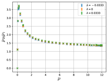
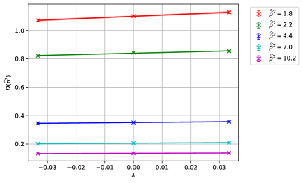
Figure 1: Left panel: $p^{2}\mbox{tr}\,D_{\lambda}(p)$ versus $p^{2}$ for $\lambda=0$, $\pm 0.0333$. Right panel: $\mbox{tr}\,D_{\lambda}(p)$ versus $\lambda$ for selected values of $p^{2}$, as given in the figure together with a linear fit (in $\lambda$). $O(1000)$ configurations per $\lambda$ value were generated.

(for $\beta=6.0$ on a $24^{3}\times 48$ lattice in the Landau gauge, $\xi=0$) against $p^{2}$ where $p=(2\pi/24)(n,n,n,0)$ i.e. with a ‘cylinder’ cut (left panel) and against $\lambda$ (right panel). From the gradients of the fits for each $p^{2}$ (some selected values are given in the right panel of Fig. 1) we can determine $Z_{g}$ as given in eq. (30). In Fig. 2 we

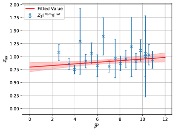
Figure 2: $Z_{g}$ as given in eq. (30) versus $p^{2}$, together with a linear fit.

we compare $Z_{g}$ determined from eq. (30) together with a linear fit $Z_{g}=A+Bp^{2}$, where the gradient term is taken to represent residual lattice effects. We find $A=0.799(91)$ for $Z_{g}$. Work is in progress to try to reduce the errors.

As a benchmark comparison from [9] we have $Z_{g}|_{g^{2}=1}=(1-1.0225g^{2}+0.1305g^{4})/(1-0.8557g^{2})|_{g^{2}=1}=0.748(20)$. (This follows from setting $Z_{g}=1-g^{2}/2(c_{\sigma}-c_{\tau})$, together with a non-perturbative determination of the anisotropic coefficients $c_{\sigma}$ and $c_{\tau}$, see also [10].) This comparison to [9] is the main result given here.

4 Conclusions and outlook

In conclusion $\langle x\rangle_{g}^{\rm\scriptscriptstyle R}$ is a notoriously difficult quantity to compute as it is a short distance quantity with numerically large fluctuations – it is a ‘disconnected quantity’. A straightforward determination requires hundreds of thousands of configurations. We have developed a FH technique, now including the renormalisation, which although several runs are required each run is only moderately expensive.

We note that it is also possible to determine $Z_{gq}$ in the same way using the FH theorem after suitably modifying the quark propagator, when

$$Z_{gq}\propto\mbox{tr}\,\Gamma^{(b)\,{\rm\scriptscriptstyle Born}}(S_{\lambda}^{-1}-S_{0}^{-1})\,.$$ (32)

Finally a few comments about a more realistic computation with $2+1$ dynamical flavours of quarks. This has a more complicated renormalisation pattern. We have the general structure

$$\left(\begin{array}[]{l}\langle x\rangle_{g}\\[1.8063pt] \langle x\rangle_{u}^{\rm\scriptscriptstyle con}\\ \langle x\rangle_{d}^{\rm\scriptscriptstyle con}\\ \langle x\rangle_{s}^{\rm\scriptscriptstyle con}\\[1.8063pt] \langle x\rangle_{u}^{\rm\scriptscriptstyle dis}\\ \langle x\rangle_{d}^{\rm\scriptscriptstyle dis}\\ \langle x\rangle_{s}^{\rm\scriptscriptstyle dis}\\ \langle x\rangle^{\rm\scriptscriptstyle con}_{q_{v}}\\ \end{array}\right)^{\rm\scriptscriptstyle R}=\left(\begin{array}[]{cccccccc}Z_{gg}&Z_{gq}&Z_{gq}&Z_{gq}&Z_{gq}&Z_{gq}&Z_{gq}&Z_{gq}\\[1.8063pt] 0&Z_{a}-Z_{b}&0&0&0&0&0&Z_{a}-Z_{b}\\ 0&0&Z_{a}-Z_{b}&0&0&0&0&Z_{a}-Z_{b}\\ 0&0&0&Z_{a}-Z_{b}&0&0&0&Z_{a}-Z_{b}\\[1.8063pt] Z_{qg}&Z_{b}&Z_{b}&Z_{b}&Z_{a}&Z_{b}&Z_{b}&Z_{b}\\ Z_{qg}&Z_{b}&Z_{b}&Z_{b}&Z_{b}&Z_{a}&Z_{b}&Z_{b}\\ Z_{qg}&Z_{b}&Z_{b}&Z_{b}&Z_{b}&Z_{b}&Z_{a}&Z_{b}\\[1.8063pt] 0&0&0&0&0&0&0&Z_{a}-Z_{b}\\ \end{array}\right)\,\left(\begin{array}[]{l}\langle x\rangle_{g}\\[1.8063pt] \langle x\rangle_{u}^{\rm\scriptscriptstyle con}\\ \langle x\rangle_{d}^{\rm\scriptscriptstyle con}\\ \langle x\rangle_{s}^{\rm\scriptscriptstyle con}\\[1.8063pt] \langle x\rangle_{u}^{\rm\scriptscriptstyle dis}\\ \langle x\rangle_{d}^{\rm\scriptscriptstyle dis}\\ \langle x\rangle_{s}^{\rm\scriptscriptstyle dis}\\ \langle x\rangle^{\rm\scriptscriptstyle con}_{q_{v}}\\ \end{array}\right)^{\rm\scriptscriptstyle lat}\,,$$ (57)

where we consider here the case of $n_{f}=3$ quarks and $n_{f_{v}}=1$ partially quenched (or valence) quarks. Practically it is easier to split the terms into quark-line-connected and -disconnected pieces, $\langle x\rangle_{q}=\langle x\rangle_{q}^{\rm\scriptscriptstyle con}+\langle x\rangle_{q}^{\rm\scriptscriptstyle dis}$ with for example $\langle x\rangle_{q}^{{\rm\scriptscriptstyle con}\,{\rm\scriptscriptstyle R}}=Z_{qq}^{\rm\scriptscriptstyle NS}\langle x\rangle_{q}^{{\rm\scriptscriptstyle con}\,{\rm\scriptscriptstyle lat}}$. All $Z$s depend on scheme and renormalisation scale $\mu$. The non-singlet (e.g. $\langle x\rangle_{u}-\langle x\rangle_{d}$) and singlet (i.e. $\langle x\rangle_{u}+\langle x\rangle_{d}+\langle x\rangle_{s}$) renormalisation constants are thus

$$Z_{qq}^{\rm\scriptscriptstyle NS}=Z_{a}-Z_{b}\,,\qquad Z_{qq}^{\rm\scriptscriptstyle S}=Z_{qq}^{\rm\scriptscriptstyle NS}+n_{f}Z_{b}\,,$$ (58)

respectively. As before we have

$$\left(\langle x\rangle_{g}+\sum_{q}\langle x\rangle_{q}+\sum_{q_{v}}\langle x\rangle_{q_{v}}\right)^{\rm\scriptscriptstyle R} = Z_{g}\langle x\rangle_{g}^{\rm\scriptscriptstyle lat}+Z_{q}\left(\sum_{q}\langle x\rangle_{q}+\sum_{q_{v}}\langle x\rangle_{q_{v}}\right)^{\rm\scriptscriptstyle lat}=1\,,$$

giving

$$Z_{g}=Z_{gg}^{\rm\scriptscriptstyle\overline{MS}}+n_{f}Z_{qg}^{\rm\scriptscriptstyle\overline{MS}}\,,\qquad Z_{q}=Z_{gq}^{\rm\scriptscriptstyle\overline{MS}}+Z_{qq}^{{\rm\scriptscriptstyle NS}\,\rm\scriptscriptstyle\overline{MS}}\,,$$

with as before $Z_{g}$, $Z_{q}$ just depending on the coupling, $g$, but individual terms depend on the chosen scheme, e.g. $\overline{MS}$. A similar FH scheme for the renormalisation is being developed here.

References

- [1] M. Göckeler et al., Nucl. Phys. Proc. Suppl. 53 (1997) 324, arXiv:hep-lat/9608017.
- [2] H. B. Meyer et al., Phys. Rev. D 77 (2008) 037501 [arXiv:0707.3225 [hep-lat]].
- [3] R. Horsley et al. [QCDSF and UKQCD Collaborations], Phys. Lett. B 714 (2012) 312 [arXiv:1205.6410 [hep-lat]].
- [4] C. Alexandrou et al., Phys. Rev. D 96 (2017) 054503 [arXiv:1611.06901 [hep-lat]].
- [5] Y. B. Yang et al. [QCD Collaboration], Phys. Rev. Lett. 121 (2018) 212001 [arXiv:1808.08677 [hep-lat]].
- [6] P. E. Shanahan et al., Phys. Rev. D 99 (2019) 014511 [arXiv:1810.04626 [hep-lat]].
- [7] A. J. Chambers et al. [QCDSF Collaboration], Phys. Lett. B 740 (2015) 30 [arXiv:1410.3078 [hep-lat]].
- [8] X. D. Ji, Phys. Rev. Lett. 74 (1995) 1071 [hep-ph/9410274].
- [9] J. Engels et al., Nucl. Phys. B 564 (2000) 303 [hep-lat/9905002].
- [10] H. B. Meyer, Phys. Rev. D 76 (2007) 101701 [arXiv:0704.1801 [hep-lat]].
- [11] M. Göckeler et al. [QCDSF Collaboration], Phys. Rev. D 71 (2005) 114511 [hep-ph/0410187].
- [12] T. R. Haar et al., EPJ Web Conf. 175 (2018) 14011, arXiv:1711.03836 [hep-lat].
- [13] R. G. Edwards et al., Nucl. Phys. Proc. Suppl. 140 (2005) 832, arXiv:hep-lat/0409003.