Adaptive Low-level Storage of Very Large Knowledge Graphs
Abstract.
The increasing availability and usage of Knowledge Graphs (KGs) on the Web calls for scalable and general-purpose solutions to store this type of data structures. We propose Trident, a novel storage architecture for very large KGs on centralized systems. Trident uses several interlinked data structures to provide fast access to nodes and edges, with the physical storage changing depending on the topology of the graph to reduce the memory footprint. In contrast to single architectures designed for single tasks, our approach offers an interface with few low-level and general-purpose primitives that can be used to implement tasks like SPARQL query answering, reasoning, or graph analytics. Our experiments show that Trident can handle graphs with edges using inexpensive hardware, delivering competitive performance on multiple workloads.
1. Introduction
Motivation. Currently, a large wealth of knowledge is published on the Web in the form of interlinked Knowledge Graphs (KGs). These KGs cover different fields (e.g., biomedicine (Noy et al., 2009; Callahan et al., 2013), encyclopedic or commonsense knowledge (Vrandečić and Krötzsch, 2014; Tandon et al., 2014), etc.), and are actively used to enhance tasks such as entity recognition (Shen et al., 2015), query answering (Yahya et al., 2016), or more in general Web search (Guha et al., 2003; Blanco et al., 2013; Greaves and Mika, 2008).
As the size of KGs keeps growing and their usefulness expands to new scenarios, applications increasingly need to access large KGs for different purposes. For instance, a search engine might need to query a KG using SPARQL (Harris et al., 2013), enrich the results using embeddings of the graph (Nickel et al., 2015), and then compute some centrality metrics for ranking the answers (Kasneci et al., 2008; Tonon et al., 2016). In such cases, the storage engine must not only efficiently handle large KGs, but also allow the execution of multiple types of computation so that the same KG does not have to be loaded in multiple systems.
Problem. In this paper, we focus on providing an efficient, scalable, and general-purpose storage solution for large KGs on centralized architectures. A large amount of recent research has focused on distributed architectures (Gonzalez et al., 2012, 2014; Han et al., 2014; Malewicz et al., 2010; Qin et al., 2014; Shao et al., 2013; Gurajada et al., 2014; Ching et al., 2015), because they offer many cores and a large storage space. However, these benefits come at the price of higher communication cost and increased system complexity (Perez et al., 2015). Moreover, sometimes distributed solutions cannot be used either due to financial or privacy-related constraints.
Centralized architectures, in contrast, do not have network costs, are commonly affordable, and provide enough resources to load all-but-the-largest graphs. Some centralized storage engines have demonstrated that they can handle large graphs, but they focus primarily on supporting one particular type of workload (e.g., Ringo (Perez et al., 2015) supports graph analytics, RDF engines like Virtuoso (OpenLink Software, 2019) or RDFox (Motik et al., 2014) focus on SPARQL (Harris et al., 2013)). To the best of our knowledge, we still lack a single storage solution that can handle very large KGs as well as support multiple workloads.
Our approach. In this paper, we fill this gap presenting Trident, a novel storage architecture that can store very large KGs on centralized architectures, support multiple workloads, such as SPARQL querying, reasoning, or graph analytics, and is resource-savvy. Therefore, it meets our goal of combining scalability and general-purpose computation.
We started the development of Trident by studying which are the most frequent access types performed during the execution of tasks like SPARQL answering, reasoning, etc. Some of these access types are node-centric (i.e., access subsets of the nodes), while others are edge-centric (i.e., access subsets of the edges). From this study, we distilled a small set of low-level primitives that can be used to implement more complex tasks. Then, the research focused on designing an architecture that supports the execution of these primitives as efficiently as possible, resulting in Trident.
At its core, Trident uses a dedicated data structure (a B+Tree or an in-memory array) to support fast access to the nodes, and a series of binary tables to store subsets of the edges. Since there can be many binary tables – possibly billions with the largest KGs – handling them with a relational DBMS can be problematic. To avoid this problem, we introduce a light-weight storage scheme where the tables are serialized on byte streams with only a little overhead per table. In this way, tables can be quickly loaded from the secondary storage without expensive pre-processing and offloaded in case the size of the database exceeds the amount of available RAM.
Another important benefit of our approach is that it allows us to exploit the topology of the graph to reduce its physical storage. To this end, we introduce a novel procedure that analyses each binary table and decides, at loading time, whether the table should be stored either in a row-by-row, column-by-column, or in a cluster-based fashion. In this way, the storage engines effectively adapts to the input. Finally, we introduce other dynamic procedures that decide, at loading time, whether some tables can be ignored due to their small sizes or whether the content of some tables can be aggregated to further reduce the space.
Since Trident offers low-level primitives, we built interfaces to several engines (RDF3X (Neumann and Weikum, 2010), VLog (Urbani et al., 2016b), SNAP (Leskovec and Sosič, 2016)) to evaluate the performance of SPARQL query answering, datalog reasoning and graph analytics on various types of graphs. Our comparison against the state-of-the-art shows that our approach can be highly competitive in multiple scenarios.
Contribution. We identified the followings as the main contributions of this paper.
-
We propose a new architecture to store very large KGs on a centralized system. In contrast to other engines that store the KG in few data structures (e.g., relational tables), our architecture exhaustively decomposes the storage in many binary tables such that it supports both node- and edge-centric via a small number of primitives;
-
Our storage solution adapts to the KG as it uses different layouts to store the binary tables depending on its topology. Moreover, some binary tables are either skipped or aggregated to save further space. The adaptation of the physical storage is, as far as we know, a unique feature which is particularly useful for highly heterogeneous graphs, such as the KGs on the Web;
-
We present an evaluation with multiple workloads and the results indicate highly competitive performance while maintaining good scalability. In some of our largest experiments, Trident was able to load and process KGs with up to (100B) edges with hardware that costs less than $5K.
The source code of Trident is freely available with an open source license at https://github.com/karmaresearch/trident, along with links to the datasets and instructions to replicate our experiments.
2. Preliminaries
A graph is a tuple where represent the sets of nodes, edges and labels respectively, is a bijection that maps each node to a label in , while is a function that maps each edge to a label in . We assume that there is at most one edge with the same label between any pair of nodes. Throughout, we use the notation to indicate the edge with label from node with label (source) to the node with label (destination).
We say that the graph is undirected if implies that also . Otherwise, the graph is directed. A graph is unlabeled if all edges map to the same label. In this paper, we will mostly focus on labeled directed graphs since undirected or unlabeled graphs are special cases of labeled directed graphs.
In practice, it is inefficient to store the graph using the raw labels as identifiers. The most common strategy, which is the one we also follow, consists of assigning a numerical ID to each label in , and stores each edge with the tuple where , , and are the IDs associated to , , and respectively.
The numerical IDs allow us to sort the edges and by permuting we can define six possible ordering criteria. We use strings of three characters over the alphabet to identify these orderings, e.g., specifies that the edges are ordered by source, relation, and destination. We denote with the collection of six orderings while specifies all partial orderings. We use the function to check whether string is a prefix of , i.e., and the operator to remove all characters of one string from another one (e.g., if and , then ).
Let be a set of variables. A simple graph pattern (or triple pattern) is an instance of and we denote it as where . A graph pattern is a finite set of simple graph patterns. Let be a partial function from variables to labels. With a slight abuse of notation, we also use as a postfix operator that replaces each occurrence of the variables in with the corresponding node. Given the graph and a simple graph pattern , the answers for on correspond to the set . Function returns the positions of the labels in the simple graph pattern left-to-right, i.e., if where and , then .
A Knowledge Graph (KG) is a directed labeled graph where nodes are entities and edges establish semantic relations between them, e.g., . Usually, KGs are published on the Web using the RDF data model (Hayes, 2004). In this model, data is represented as a set of triples of the form drawn from where denote sets of IRIs, blank nodes and literals respectively. Let be the set of all RDF terms. RDF triples can be trivially seen as a graph where the subjects and objects are the nodes, triples map to edges labeled with their predicate name, and .
SPARQL (Harris et al., 2013) is a language for querying knowledge graphs which has been standardized by W3C. It offers many SQL-like operators like UNION, FILTER, DISTINCT to specify complex queries and to further process the answers. Every query contains at its core a graph pattern, which is called Basic Graph Pattern (BGP) in the SPARQL terminology. SPARQL graph patterns are defined over and their answers are mappings from to . Therefore, answering a SPARQL graph pattern over a KG corresponds to computing and retrieving the corresponding labels.
Example 0.
An example of a SPARQL query is:
SELECT ?s ?o { ?s isA ?o . ?s livesIn Rome . }
If the KG contains the RDF triples and then one answer to the query is .
3. Graph Primitives
We start our discussion with a description of the low-level primitives that we wish to support. We distilled these primitives considering four types of workloads: SPARQL (Harris et al., 2013) query answering, which is the most popular language for querying KGs; Rule-based reasoning (Antoniou et al., 2018), which is an important task in the Semantic Web to infer new knowledge from KGs; Algorithms for graph analytics, or network analysis, since these are widely applied on KGs either to study characteristics like the graph’s topology or degree distribution, or within more complex pipelines; Statistical relational models (Nickel et al., 2015), which are effective techniques to make predictions using the KG as prior evidence.
If we take a closer look at the computation performed in these tasks, we can make a first broad distinction between edge-centric and node-centric operations. The first ones can be defined as operations that retrieve subsets of edges that satisfy some constraints. In contrast, operations of the second type retrieve various data about the nodes, like their degree. Some tasks, like SPARQL query answering, depend more heavily on edge-centric operations while others depend more on node-centric operations (e.g., random walks).
Graph Primitives. Following a RISC-like approach, we identified a small number of low-level primitives that can act as basic building blocks for implementing both node- and edge-centric operations. These primitives are reported in Table 1 and are described below.
| Name | Output | |
|---|---|---|
| Label of node (equals to ). | ||
| Label of edge (equals to ). | ||
| , i.e., the ID of node with label . | ||
| , i.e., the ID of edge label . | ||
| sorted by . | ||
| sorted by . | ||
| sorted by . | ||
| sorted by . | ||
| sorted by . | ||
| sorted by . | ||
| All of . | ||
| All of . | ||
| All of . | ||
| Aggr. / of . | ||
| Aggr. / of . | ||
| Aggr. / of . | ||
| Cardinality of . | ||
| edge returned by . | ||
| edge returned by . | ||
| edge returned by . | ||
| edge returned by . | ||
| edge returned by . | ||
| edge returned by . |
. These primitives retrieve the numerical IDs associated with labels and vice-versa. The primitives and retrieve the labels associated with nodes and edges respectively. The primitives and retrieve the labels associated with numerical IDs.
. Function retrieves the subset of the edges in that matches the simple graph pattern and returns it sorted according to . Primitives in this group are particularly important for the execution of SPARQL queries since they encode the core operation of retrieving the answers of a SPARQL triple pattern.
. This group of primitives returns an aggregated version of the output of . For instance, returns the list of all distinct sources in the edges with the respective counts of the edges that share them. Let be a set of edges, and . Then, returns the list of all tuples in sorted by the numerical ID of the first field. The other primitives are defined analogously.
. This primitive returns the cardinality of the output of . This computation is useful in a number of cases: For instance, it can be used to optimize the computation of SPARQL queries by rearranging the join ordering depending on the cardinalities of the triple patterns or to compute the degree of nodes in the graph.
. These primitives return the edge that would be returned by the corresponding primitives . In practice, this operation is needed in several graph analytics algorithms or for mini-batching during the training of statistical relational models.
Example 0.
We show how we can use the primitives in Table 1 to answer the SPARQL query of Example 2.1, assuming that the KG is called .
-
First, we retrieve the IDs of the labels , , and . To this end, we can use the primitives and .
-
Then, we create two single graph patterns and which map to the first and second triple patterns respectively. Then, we execute and so that the edges are returned in a order suitable for a merge join.
-
We invoke the primitive to retrieve all the labels of the nodes which are returned by the join algorithm. These labels are then used to construct the answers of the query.
4. Architecture
One straightforward way to implement the primitives in Table 1 is to store the KG in many independent data structures that provide optimal access for each function. However, such solution will require a large amount of space and updates will be slow. It is challenging to design a storage engine that uses fewer data structures without excessively compromising the performance.
Moreover, KGs are highly heterogeneous objects where some subgraphs have a completely different topology than others. The storage engine should take advantage of this diversity and potentially store different parts of the KGs in different ways, effectively adapting to its structure. This adaptation lacks in current engines, which treat the KG as a single object to store.
Our architecture addresses these two problems with a compact storage layer that supports the execution of primitives with a minimal compromise in terms of performance, and in such a way that the engine can adapt to the KG in input selecting the best strategy to store its parts.
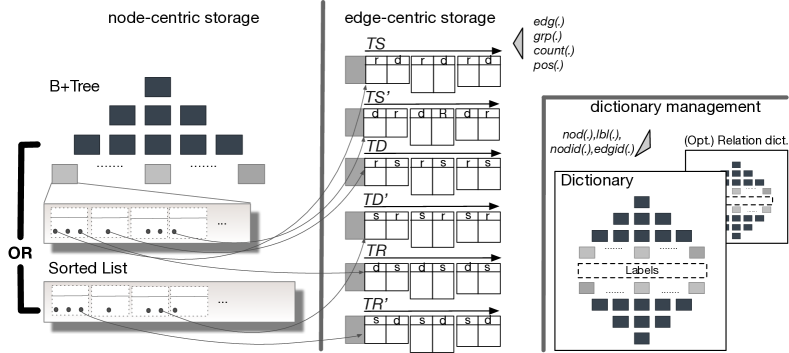
Figure 1 gives a graphical view of our approach. It uses a series of interlinked data structures that can be grouped in three components. The first one contains data structures for the mappings . The second component is called edge-centric storage and contains data structures for providing fast access to the edges. The third one is called node-centric storage and offers fast access to the nodes. Section 4.1 describes these components in more detail. Section 4.2 discusses how they allow an efficient execution of the primitives, while Section 4.3 focuses on loading and updating the database.
4.1. Architectural Components
Dictionary. We store the labels on a block-based byte stream on disk. We use one B+Tree called to index the mappings and another one called for . Using B+Trees here is usual, so we will not discuss it further. It is important to note that assigning a certain ID to a term rather than another one might have a significant impact on the performance. For instance, Urbani et al. (Urbani et al., 2016a) have shown that a careful choice of the IDs can introduce importance speedups due to the improved data locality. Typically, current graph engines assign unique IDs to all labels, irrespectively whether a label is used as an entity or as a relation. This is desirable for SPARQL query answering because all data joins can operate on the IDs directly. There are cases, however, where unique ID assignments are not optimal. For instance, most implementations of techniques for creating KG embeddings (e.g., TranSE (Bordes et al., 2013)) store the embeddings for the entities and the ones for relations in two contiguous vectors, and use offsets in the vectors as IDs. If the labels for the relations share the IDs with the entities, then the two vectors must have the same number of elements. This is highly inefficient because KGs have many fewer relations than entities which means that much space in the second vector will be unused. To avoid this problem, we can assign IDs to entities and relationships in an independent manner. In this way, no space is wasted in storing the embeddings. Note that Trident supports both global ID assignments and independent entity/relationship assignments with an additional index specifically for the relation labels. The first type of assignment is needed for tasks like SPARQL query answering while the second is useful for operations like learning graph embeddings (Nickel et al., 2015).
Edge-centric storage. In order to adapt to the complex and non-uniform topology of current KGs, we do not store all edges in a single data structure, but store subsets of the edges independently. These subsets correspond the edges which share a specific entity/relation. More specifically, let us assume that we must store the graph . For each , we consider three types of subsets: , , , i.e., the subsets of edges that have as source, edge, or destination respectively.
The choice of separating the storage of various subsets allows us to choose the best data structure for a specific subset, but it hinders the execution of inter-table scans, i.e., scans where the content of multiple tables must be taken into account. To alleviate this problem, we organize the physical storage in such a way that all edges can still be retrieved by scanning a contiguous memory location.
We proceed as follows: First, we compute , , for every . Let be the collection of all these sets. For each , we construct two sets of tuples, and , by extracting the free fields left-to-right and right-to-left respectively. For instance, the set results into the sets and . Since these sets contains pairs of elements, we view them as binary tables. These are grouped into the following six sets:
-
and
-
and
-
and
The content of these six sets is serialized on disk in corresponding byte streams called , , , , , and respectively (see middle section of Figure 1). The serialization is done by first sorting the binary tables by their defining label IDs, and then serializing each table one-by-one. For instance, if , then is serialized before iff . At the beginning of the byte stream, we store the list of all IDs associated to the tables, pointers to the tables’ physical location and instructions to parse them.
Since the binary tables and tuples are serialized on the byte stream with a specific order, we can retrieve all edges sorted with any ordering in with a single scan of the corresponding byte stream, using the content stored at the beginning of the stream to decode the binary tables in it. For instance, we can scan to retrieve all edges sorted according to . The IDs stored at the beginning of the stream specify the sources of the edges () while the content of the tables specify the remaining relations and destinations (and ).
Node-centric storage. In order to provide fast access to the nodes, we map each ID (i.e., the ID assigned to label ) to a tuple that contains 15 fields:
-
the cardinalities , , and ;
-
Six pointers to the physical storage of , , , , , and ;
-
Six bytes that contain instructions to read the data structures pointed by . These instructions are necessary because the tables are stored in different ways (see Section 5).
We index all tuples by the numerical IDs using one global data structure called (Node Manager), shown on the left side of Figure 1. This data structure is implemented either with an on-disk B+Tree or with a in-memory sorted vector (the choice is done at loading time). The B+Tree is preferable if the engine is used for edge-based computation because the B+Tree does not need to load all nodes in main memory and the nodes are accessed infrequently anyway. In contrast, the sorted vector provides much faster access ( vs. ) but it requires that the entire vector is stored in main memory. Thus, it is suitable only if the application accesses the nodes very frequently and there are enough hardware resources.
Note that the coordinates to the binary tables are stored both in and in the meta-data in front of the byte streams. This means that the table can be accessed either by accessing , or by scanning the beginning of the byte stream. In our implementation, we consult when we need to answers graph patterns with at least one constant element (e.g., for answering the query in Example 2.1). In contrast, the meta-content at the beginning of the stream is used when must perform a full scan.
The way we store the binary tables in six byte streams resembles six-permutation indexing schemes such as proposed in engines like RDF3X (Neumann and Weikum, 2010) or Hexastore (Weiss et al., 2008). There are, however, two important differences: First, in our approach the edges are stored in multiple independent binary tables rather than a single series of ternary tuples (as, for instance, in RDF3X (Neumann and Weikum, 2010)). This division is important because it allows us to choose different serialization strategies for subgraphs or to avoid storing some tables (Section 5.3). The second difference is that in our case most access patterns go through a single B+Tree instead of six different data structures. This allows us to save space and to store additional information about the nodes, e.g., their degree, which is useful, for instance, for traversal algorithms like PageRank, or random walks.
4.2. Primitive Execution
We now discuss how we can implement the primitives in Table 1 with our architecture.
. These are executed consulting either or . Thus, the time complexity follows in a straightforward manner.
Proposition 0.
Let . The time complexity of computing is .
. Let be a generic invocation of one of . First, we need to retrieve the numerical IDs associated to the labels in (if any). Then, we select an ordering that allows us to 1) retrieve answers for with a range scan, and 2) the ordering complies with . The orderings that satisfy 1) are
| (1) |
An ordering which also satisfies 2) is one for which .
Example 0.
Consider the execution of where . In this case, , and .
The selected is associated to one byte stream. If contains one or more constants, then we can query to retrieve the appropriate binary table from that binary stream and (range-)scan it to retrieve the answers of . In contrast, if only contains variables, the results can be obtained by scanning all tables in the byte stream. Note that the cost of retrieving the IDs for the labels in is since we use B+Trees for the dictionary. This is an operation that is applied any time the input contains a graph pattern. If we ignore this cost and look at the remaining computation, then we can make the following observation.
Proposition 0.
Let . The time complexity of is if only contains variables, otherwise.
. Let be a general call to one of these primitives. Note that in this case , i.e., is a partial ordering. These functions can be implemented by invoking and then return an aggregated version. Thus, they have the same cost as the previous ones.
However, there are special cases where the computation is quicker, as shown in the next example.
Example 0.
Consider a call to where . In this case, we can query with and return at most one tuple with the cardinality stored in , which has a cost of O(log(|L|)).
If has length two or contains a repeated variable, then we also need to access one or more binary tables, similarly as before.
Proposition 0.
Let . The time complexity of ranges between and depending on and .
. This primitive returns the cardinality of the output of . Therefore, it can be simply implemented by iterating over the results returned by these functions. However, there there are cases when we can avoid this iteration. Some of such cases are the ones below:
-
If the input is and contains no constant nor repeated variables. In this case the output is .
-
If the input is and contains only one constant and no repeated variables. In this case the cardinality is stored in .
-
If the input is , , and contains at most one constant and no repeated variables, then the output can be obtained either by consulting or the metadata of one of the byte streams.
Otherwise, we also need to access one binary table to compute the results, which, in the worst case, takes .
Proposition 0.
Let . The time complexity of executing ranges between and .
. In order to efficiently support these primitives, we need to provide a fast random access to the edges. Given a generic , we distinguish four cases:
-
C1 If contains repeated variables, then we iterate over the results and return the edge;
-
C2 If contains only one constant, then the search space is restricted to a single binary table. In this case, the computation depends on how the content of the table is serialized on the byte stream. If it allows random access to the rows, then the cost reduces to , i.e., query . Otherwise we also need to iterate through the table and count until the row;
-
C3 If contains more than one constant, then we need to search through the table for the right interval, and then scan until we retrieve the row;
-
C4 Finally, if does not contain any constants or repeated variables, we must consider all edges stored in one byte stream. In this case, we first search for the binary table that contains the edge. This operation requires a scan of the metadata associated to the byte stream, which can take up to . Then, the complexity depends on whether the physical storage of the table allows a random access, as in C2 and C3. Since a scan over the metadata takes , this last case represents the worst-case in terms of complexity as it sums to . Note that in this case, simply going through all edges is faster as it takes . However, in practice tables have more than one row so we can advance more quickly despite the higher worst-case complexity.
Proposition 0.
Let . The time complexity of executing ranges between and .
4.3. Bulk Loading and Updates
Bulk Loading. Loading a large KG can be a lengthy process, especially if the resources are constrained. In Trident, we developed a loading routine which exploits the multi-core architecture and maximizes the (limited) I/O bandwidth.
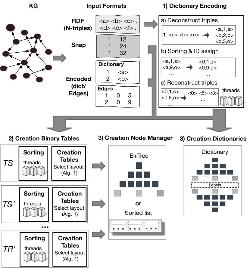
The main operations are shown in Figure 2. Our implementation can receive the input KG in multiple formats. Currently, we considered the N-Triples format (popular in the Semantic Web) and the SNAP format (Leskovec and Krevl, 2014) (used for generic graphs). The first operation is encoding the graph, i.e., assigning unique IDs to the entities and relation labels. For this task, we adapted the MapReduce technique presented at (Urbani et al., 2013) to work in a multi-core environment. This technique first deconstructs the triples, then assigns unique IDs to all the terms, and finally reconstruct the triples. If the graph is already encoded, then our procedure skips the encoding and proceeds to the second operation of the loading, the creation of the database.
The creation of the binary tables requires that the triples are pre-sorted according to a given ordering. We use a disk-based parallel merge sort algorithm for this purpose. The tables are serialized one-by-one selecting the most efficient layout for each of them. After all the tables are created, the loading procedure will create the and the B+Trees with the dictionaries. The encoding and sorting procedures are parallelized using threads, which might need to communicate with the secondary storage. Modern architectures can have >64 cores, but such a number of threads can easily saturate the disk bandwidth and cause serious slowdowns. To avoid this problem, we have two types of threads: Processing threads, which perform computation like sorting, and I/O threads, which only read and write from disk. In this way, we can control the maximum number of concurrent accesses to the disks.
Updates. To avoid a complete re-loading of the entire KG after each change, our implementation supports incremental updates. Our procedure is built following the well-known advice by Jim Gray (Gray, 1981) that discourages in-place updates, and it is inspired by the idea of differential indexing (Neumann and Weikum, 2010), which proposes to create additional indices and perform a lazy merging with the main database when the number of indices becomes too high.
Our procedure first encodes the update, which can be either an addition or removal, and then stores it in a smaller “delta” database with its own and byte streams. Multiple updates will be stored in multiple databases, which are timestamped to remember the order of updates. Also, updates create an extra dictionary if they introduce new terms. Whenever the primitives are executed, the content of the updates is combined with the main KG so that the execution returns an updated view of the graph.
In contrast to differential indexing, our merging does not copy the updates in the main database, but only groups them in two updates, one for the additions and one for the removals. This is to avoid the process of rebuilding binary tables with possibly different layouts. If the size of the merged updates becomes too large, then we proceed with a full reload of the entire database.
5. Adaptive Storage Layout
The binary tables can be serialized in different ways. For instance, we can store them row-by-row or column-by-column. Using a single serialization strategy for the entire KG is inefficient because the tables can be very different from each other, so one strategy may be efficient with one table but inefficient with another. Our approach addresses this inefficiency by choosing the best serialization strategy for each table depending on its size and content.
For example, consider two tables and . Table contains all the edges with label “isA”, while contains all the edges with label “isbnValue”. These two tables are not only different in terms of sizes, but also in the number of duplicated values. In fact, the second column of is likely to contain many more duplicate values than the second column of because there are (typically) many more instances than classes while “isbnValue” is a functional property, which means that every entity in the first column is associated with a unique ISBN code. In this case, it makes sense to serialize in a column-by-column fashion so that we can apply run-length-encoding (RLE) (Abadi et al., 2006), a well-known compression scheme of repeated values, to save space when storing the second column. This type of compression would be ineffective with since there each value appears only once. Therefore, can be stored row-by-row.
In our approach, we consider three different serialization strategies, which we call serialization layouts (or simply layouts) and employ an ad-hoc procedure to select, for each binary table, the best layout among these three.
5.1. Serialization Layouts
We refer to the three layouts that we consider as row, column, and cluster layouts respectively. The first layout stores the content row-by-row, the second column-by-column, while the third uses an intermediate representation.
Row layout. Let be a binary table that contains sorted pairs of elements. With this layout, the pairs are stored one after the other. In terms of space consumption, this layout is optimal if the two columns do not contain any duplicated value. Moreover, if each row takes a fixed number of bytes, then it is possible to perform binary search or perform a random access to a subset of rows. The disadvantage is that with this layout all values are explicitly written on the stream while the other layouts allow us to compress duplicate values.
Column layout. With this layout, the elements in are serialized as . The space consumption required by this layout is equal to the previous one but with the difference that here we can use RLE to reduce the space of . In fact, if , then we can simply write . Also this layout allows binary search and a random access to the table. However, it is slightly less efficient than the row layout for full scans because here one row is not stored at contiguous locations, and the system needs to “jump” between columns in order to return the entire pair. On the other hand, this layout is more suitable than the row layout for aggregate reads (required, for instance, for executing primitives) because in this case we only need to read the content of one column which is stored at contiguous locations.
Cluster layout. Let be the longest sub-sequence of pairs in which share the first term . With this layout, all groups are first ordered in the sequence such that for all . Then, they are serialized one-by-one. Each group is serialized by first writing , then , and finally the list . This layout needs less space than the row layout if the groups contain multiple elements. Otherwise, it uses more space because it also stores the size of the groups, and this takes an extra bits. Another disadvantage is that with this layout binary search is only possible within one group.
5.2. Dynamic Layout Selection
The procedure for selecting the best layout for each table is reported in Algorithm 1. Its goal is to select the layout which leads to the best compression without excessively compromising the performance. In our implementation, Algorithm 1 is applied by default, but the user can disable it and use one layout for all tables.
The procedure receives as input a binary table with rows and returns a tuple that specifies the layout that should be chosen. It proceeds as follows. First, it makes a distinction between tables that have less than rows (default value of is 1M) and contain less than unique elements in the first column from tables that do not (line 2). We make this distinction because 1) if the number of rows is too high then searching for the most optimal layout becomes expensive and 2) if the number of unique pairs is too high, then the cluster layout should not be used due to the lack of support of binary search. With small tables, this is not a problem because it is well known that in these cases linear search is faster than binary search due to a better usage of the CPU’s cache memory. The value for is automatically determined with a small routine that performs some micro-benchmarks to identify the threshold after which binary search becomes faster. In our experiments, this value ranged between 16 and 64 elements.
If the table satisfies the condition of line 2, then the algorithm selects either the or the layout. The layout is not considered because its main benefit against the other two is a better compression (e.g., RLE) but this is anyway limited if the table is small. The procedure scans the table and keeps track of the largest numbers and groups used in the table (). Then, the function invokes the subroutine to retrieve the number of bytes needed to store these numbers. It uses this information to compute the total number of bytes that would be needed to store the table with the and layout respectively (variables and ). Then, it selects the layout that leads to maximum compression.
If the condition in line 2 fails, then either the or the layout can be selected. An exact computation would be too expensive given the size of the table. Therefore, we always choose since the other one cannot be compressed with RLE.
Next to choosing the best layout, Algorithm 1 also returns the maximum number of bytes needed to store the values in the two fields in the table ( and ) and (optionally) also for storing the cluster size (, this last value is only needed for ). The reason for doing so is that it would be wasteful to use four- or eight-byte integers to store small IDs. In the worst case, we assume that all IDs in both fields can be stored with five bytes, which means it can store up to terms. We decided to use byte-wise compression rather than bit-wise compression because the latter does not appear to be worthwhile (Neumann and Weikum, 2010). Note that more complex compression schemes could also be used (e.g., VByte (Williams and Zobel, 1999)) but this should be seen as future work.
The tuple returned by contains the information necessary to properly read the content of the table from the byte stream. The first field is the chosen layout while the other fields are the number of bytes that should be used to store the entries of the table. We store this tuple both in (in one of the fields) and at the beginning of the byte stream.
5.3. Table Pruning
With Algorithm 1, the system adapts to the KG while storing a single table. We discuss two other forms of compression that consider multiple tables and decide whether some tables should be skipped or stored in aggregated form.
On-the-fly reconstruction (OFR). Every table in one stream maps to another table in where the first column is swapped with the second column. If the tables are sufficiently small, one of them can be re-constructed on-the-fly from the other whenever needed. While this operation introduces some computational overhead, the saving in terms of space may justify it. Furthermore, the overhead can be limited to the first access by serializing the table on disk after the first re-construction.
We refer to this strategy as on-the-fly reconstruction (OFR). If the user selects it at loading time, the system will not store any binary table in which has less than rows, being a value passed by the user (default value is 20, determined after microbenchmarking).
Aggregate Indexing. Finally, we can construct aggregate indices to further reduce the storage space. The usage of aggregate indices is not novel for KG storage (Weiss et al., 2008). Here, we limit their usage to the tables in if they lead to a storage space reduction.
To illustrate the main idea, consider a generic table that contains the set of tuples . This table stores all the pairs of the triples with the predicate . Since there are typically many more instances than classes, the first column of (the classes) will contain many duplicate values. If we range-partition with the first field, then we can identify a copy of the values in the second field of in the partitions of tables in where the first term is . With this technique, we avoid storing the same sequence of values twice but instead store a pointer to the partition in the other table.
6. Evaluation
| Type | #Edges | #Nodes | Type | #Edges | #Nodes | ||
|---|---|---|---|---|---|---|---|
| KG | Var. | Var. | KG | 76M | 37M | ||
| KG | 1B | 233M | Dir. | 5.1M | 875k | ||
| KG | 1.1B | 299M | Dir. | 1.7M | 81k | ||
| KG | 168M | 177M | Undi. | 198k | 18k | ||
| KG | 1B | 367M |
Trident is developed in C++, is freely available, and works under Windows, Linux, MacOS. Trident is also released in the form of a Docker image. The user can interact via command line, web interface, or HTTP requests according to the SPARQL standard.
| Graph triple patterns | |||||
|---|---|---|---|---|---|
| 0 | 1 | 2 | 3 | 4 | |
| Default | 1.28s | 0.07s | 0.15s | 0.14s | 0.18s |
| With | 1.76s | 0.07s | 0.38s | 0.38s | 0.30s |
| With | 1.30s | 0.07s | 0.16s | 0.14s | 0.19s |
| Only | 1.25s | 0.07s | 0.16s | 0.16s | 0.15s |
| Only | 1.82s | 0.07s | 0.22s | 0.18s | 0.27s |
| RDF3X | 0.70s | 0.06s | 22.84s | 26.53s | 18.55s |
| Default | With | With | With |
| 3.9GB | 2.7GB | 3.4GB | 2.5GB |
| RDF3X: 5.1GB TripleBit: 3.3GB SYSTEM_A: 6.3GB | |||
Integration with other systems. Since our system offers low-level primitives, we integrated it with the following other engines with simple wrappers to evaluate our engine in multiple scenarios:
-
RDF3X (Neumann and Weikum, 2010). RDF3X is one of the fastest and most well-known SPARQL engines. We replaced its storage layer with ours so that we can reuse its SPARQL operators and query optimizations.
-
SNAP (Leskovec and Sosič, 2016). Stanford Network Analysis Platform (SNAP) is a high-performance open-source library to execute over 100 different graph algorithms. As with RDF3X, we removed the SNAP storage layer and added an interface to our own engine.
-
VLog (Urbani et al., 2016b). VLog is one of most scalable datalog reasoners. We implemented an interface allowing VLog to reason using our system as underlying database.
We also implemented a native procedure to answer basic graph patterns (BGPs) that applies greedy query optimization based on cardinalities, and uses either merge joins or index loop joins if the first cannot be used.
Testbed. We used a Linux machine (kernel 3.10, GCC 6.4, page size 4k) with dual Intel E5-2630v3 eight-core CPUs of 2.4 GHz, 64 GB of memory and two 4TB SATA hard disks in RAID-0 mode. The commercial value is well below $5K. We compared against RDF3X and SNAP with their native storages, TripleBit (Yuan et al., 2013), a in-memory state-of-the-art RDF database (in contrast to RDF3X which uses disks), and SYSTEM_A, a widely used commercial SPARQL engine111We hide the real name as it is a commercial product, as usual in database research.. As inputs, we considered a selection of real-world and artifical KGs, and other non-KG graphs from SNAP (Leskovec and Krevl, 2014) (see Table 2 for statistics).
-
KGs. (Guo et al., 2005), a well-known artificial benchmark that creates KGs of arbitrary sizes. The KG is in the domain of universities and each university contributes ca. 100k new triples. Henceforth, we write to indicate a KG with universities, e.g. LUBM10 contains 1M triples; (Bizer et al., 2009), YAGO2S (Suchanek et al., 2008) and (Vrandečić and Krötzsch, 2014), three widely used KGs with encyclopedic knowledge; (Redaschi and Consortium, 2009), a KG that contains biomedical knowledge, and (Harth, 2012), a collection of crawled interlinked KGs.
-
Other graphs. We considered the graphs: , a Web graph from Google, , which contains a social circle, and , a collaboration network in Physics.
Trident was configured to use the B+Tree for and table pruning was disabled, unless otherwise stated.
6.1. Lookups
| Type Patt/ | Example | N. | Avg. # |
| Ordering(s) | Pattern | Queries | Results |
| 0/ | X Y Z | 1 | 75,999,246 |
| 1/- | X | 1 | 8,617,963 |
| 1/- | X | 1 | 29,835,479 |
| 1/- | X | 1 | 99 |
| 2/- | a X Y | 8,617,963 | 8 |
| 2/- | X Y a | 29,835,479 | 2 |
| 2/- | X a Y | 99 | 767,669 |
| 3/- | a X / a X | 8,617,963 | 4/8 |
| 3/- | X a / X a | 29,835,479 | 1/2 |
| 3/- | a X / X a | 99 | 369,011/423,335 |
| 4/- | a b X | 41,910,232 | 1 |
| 4/- | a X b | 36,532,121 | 2 |
| 4/- | X b a | 69,564,969 | 1 |
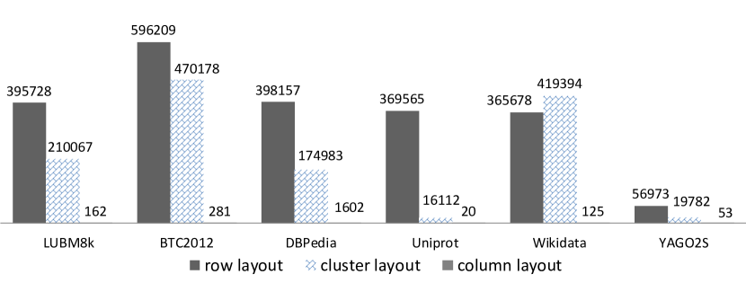
During the loading procedure, Trident applies Algorithm 1 to determine the best layout for each table. Figure 3(a) shows the number of tables of each type for the KGs. The vast majority of tables is stored either with the or layout. Only a few tables are stored with the layout. These are mostly the ones in the and byte streams. It is interesting to note that the number of tables varies differently among different KGs. For instance, the number of row tables is twice the number of cluster tables with LUBM. In contrast, with Wikidata there are more cluster tables than row ones. These differences show to what extent Trident adapted its physical storage to the structure of the KG.
One key operation of our system is to retrieve answers of simple triple patterns. First, we generated all possible triple patterns that return non-empty answers from . We considered five types of patterns. Patterns of type 0 are full scans; of type 2 contain one constants and two variables (e.g., ), while of type 4 contain two constants and one variable (e.g., ). These patterns are answered with . Patterns of types 1 request an aggregated version of a full scan (e.g., retrieve all subjects) while patterns of type 3 request an aggregation where the pattern contains one constant (e.g., return all objects of the predicate type). These two patterns are answered with .
The number, types of patterns, and average number of answers per type is reported in Table 3. The first column reports the type of pattern and the orderings we can apply when we retrieve it. The second column reports an example pattern of this type. The third column contains the number of different queries that we can construct of this type. The fourth column reports the average number of answers that we get if we execute queries of this type.
For example, the first row describes the pattern of type 0, which is a full scan. For this type of pattern, we can retrieve the answers with all the orderings in . There is only one possible query of this type (column 3) and if we execute it then we obtain about 76M answers (column 4). Patterns of type 1 correspond to full aggregated scans. An example pattern of this type is shown in the second row. If this query is executed, the system will return the list of all subjects with the count of triples that share each subject. With this input, this query will return about 8M results (i.e., the number of subjects). We can construct a similar query if we consider the variables in the second or third position. Details for these two cases are reported in the third and fourth rows.
Patterns of type 2 have one constant and two variables. Like before the constant can appear in three positions. Note that in this case we can construct many more queries by using different constants. For instance, we can construct 8.6M queries if the constant appears as subject, and 99 if it appears as predicate. Similarly, Table 3 reports such details also for queries of type 3 and 4. By testing our system on all these types of patterns, we are effectively evaluating the performance over all possible queries of these types which would return non-empty answers.
We used the primitives to retrieve the answers for these patterns with various configurations of our system, and compared against , which was the system with fastest runtimes. The median warm runtimes of all executions are reported in Figure 3(c).
The row “Default” reports the results with the adaptive storage selected by Algorithm 1 but without table pruning. The rows “With ” and “With ” use Algorithm 1 and the two techniques for table pruning discussed in Section 5.3 respectively. The rows “Only ()” use only the and layouts (the is not competitive alone due to the lack of binary search). From the table, we see that if the two pruning strategies are enabled, then the runtimes increase, especially with . This was expected since these two techniques trade speed for space. Their benefit is that they reduce the size of the database, as shown in Figure 3(c). In particular, is very effective, and they can reduce the size by 35%. Therefore, they should only be used if space is critical. The layout returns competitive performance if used alone but then the database size is about 9% larger due to the suboptimal compression. Figure 3(c) also reports the size of the databases with the other systems as reference. Note that the reported numbers for Trident do not include the size of the dictionary (764MB). This size should be added to the reported numbers for a fair comparison with the other systems’ databases.
A comparison against shows that the latter is faster with full scans (patterns of type 0) because our approach has to visit more tables stored with different configurations. However, our approach has comparable performance with the second pattern type and performs significantly better when the scan is limited to a single table, with, in the best case, improvements of more than two orders of magnitude (pattern 3). Note that in contexts like SPARQL query answering, patterns that contain at least one constant are much more frequent than full scans (e.g., see Table 2 of (Rietveld and Hoekstra, 2014)).
| Q. | N. Query | Cold runtime (ms.) | Warm runtime (ms.) | |||||||||
|---|---|---|---|---|---|---|---|---|---|---|---|---|
| Answers | TN | TR | R3X | TripleBit | SYSTEM_A | TN | TR | R3X | TripleBit | SYSTEM_A | ||
| LUBM1B | 1 | 10 | 136.165 | 50.839 | 186.127 | 61.78 | 956.34 | 0.107 | 0.164 | 1.331 | 11.76 | 0.39 |
| 2 | 10 | 307.625 | 3,182 | 174.040 | x | 10,620 | 0.181 | 1,067 | 3.528 | x | 0.33 | |
| 3 | 0 | 807,870 | 6,468 | 712,365 | 0.31 | 24,538 | 806,194 | 2,387 | 701,738 | 0.04 | 9,365 | |
| 4 | 2,528 | 643,072 | 24,848 | 738,473 | 20,308 | 49,816 | 611,083 | 19,435 | 709,541 | 20,298 | 9,244 | |
| 5 | 351,919 | 9,801 | 25,694 | 105,386 | 15,352 | 171,850 | 4,704 | 14,452 | 22,468 | 12,212 | 150,407 | |
| Uniprot | 1 | 853 | 469.759 | 643.739 | 2,969 | 141.76 | 8,532 | 1.245 | 8.676 | 15.058 | 2.347 | 17.145 |
| 2 | 32 | 371.790 | 1,475 | 267.184 | 64.00 | 2,767 | 0.168 | 52.000 | 4.144 | 0.545 | 1.121 | |
| 3 | 10,715,646 | 20,557 | 9,660 | 132,966 | 8,224 | 189,962 | 17,729 | 7,318 | 64,923 | 6,532 | 96,063 | |
| 4 | 5,564 | 1,355 | 3,469 | 1,474 | 352.70 | 4,112 | 17.025 | 438.864 | 50.898 | 211.71 | 58.498 | |
| 5 | 0 | 78.583 | 892.596 | 168.806 | x | 770.707 | 2.759 | 298.881 | 2.489 | x | 1.226 | |
| DBPEDIA | 1 | 449 | 537.754 | 885.549 | 687.848 | 46.93 | 2,706 | 0.632 | 80.511 | 21.157 | 3.14 | 25.86 |
| 2 | 600 | 249.147 | 306.902 | 354.489 | 127.17 | 1,675 | 0.075 | 0.118 | 3.533 | 0.58 | 4.47 | |
| 3 | 270 | 472.855 | 562.649 | 756.241 | 71.22 | 2,091 | 0.436 | 7.761 | 9.356 | 0.92 | 3.22 | |
| 4 | 68 | 869.719 | 1,445 | 1,128 | 116.60 | 6,233 | 0.371 | 124.391 | 9.600 | 1.42 | 4.32 | |
| 5 | 1,643 | 433.677 | 811.409 | 4,705 | 355.93 | 10,055 | 5.158 | 24.207 | 31.842 | 8.89 | 47.46 | |
| BTC2012 | 1 | 0 | 23.828 | 24.260 | 297.849 | 127.25 | N.A. | 0.069 | 0.050 | 4.903 | 0.99 | N.A. |
| 2 | 1 | 355.780 | 607.617 | 185.877 | 65.48 | N.A. | 0.197 | 24.911 | 6.279 | 0.55 | N.A. | |
| 3 | 1 | 415.230 | 1,515 | 506.125 | 244.29 | N.A. | 0.257 | 116.572 | 18.896 | 1.80 | N.A. | |
| 4 | 664 | 1,340 | 2,914 | 4,773 | 1,000 | N.A. | 24.693 | 1,049 | 290.655 | 75.98 | N.A. | |
| 5 | 5,996 | 6,120 | 19,525 | 4,446 | 3,404 | N.A. | 5.493 | 9,410 | 528.668 | 18.95 | N.A. | |
| WIKIDATA | 1 | 43 | 174.608 | 248.589 | 706.03 | 29.72 | N.A. | 0.183 | 0.386 | 2.278 | 0.505 | N.A. |
| 2 | 55 | 154.305 | 189.611 | 851.00 | 32.94 | N.A. | 0.066 | 0.063 | 1.081 | 0.107 | N.A. | |
| 3 | 1,583 | 578.537 | 873.176 | 327.25 | 522.03 | N.A. | 4.095 | 140.315 | 52.731 | 57.054 | N.A. | |
| 4 | 682 | 355.267 | 742.303 | 5,461 | 232.02 | N.A. | 24.110 | 27.627 | 179.36 | 15.219 | N.A. | |
| 5 | 1,975,090 | 2,013 | 1,995 | 75,810 | 2,946 | N.A. | 817.614 | 728.641 | 6,399 | 1,533 | N.A. | |
6.2. SPARQL
Table 4 reports the average of five cold and warm runtimes with our system and with other state-of-the-art engines. For , , , and , we considered queries used to evaluate previous systems (Yuan et al., 2013). For Wikidata, we designed five example queries of various complexity looking at published examples. The queries are reported in Appendix A. Unfortunately, we could not load and with SYSTEM_A due to raised exceptions during the loading phase.
We can make a few observations from the obtained results. First, a direct comparison against is problematic because sometimes crashed or returned wrong results (checked after manual inspection). Looking at the other systems, we observe that our approach returned the best cold runtimes for 20 out of 25 queries, counting in both the executions with our native SPARQL engine and the integration with RDF3X. If we compare the warm runtimes, our system is faster 20 out of 25 times. Furthermore, we observe that Trident/N is faster than Trident/R mostly with selective queries that require only a few joins. Otherwise the second is faster. The reason is that uses a sophisticated query optimizer that builds multiple plans in a bottom-up fashion. This procedure is costly if applied to simple queries, but it pays off for more complex ones because it can detect a better execution plan.
6.3. Graph Analytics, Reasoning, Learning
| ASTRO | ||||||
|---|---|---|---|---|---|---|
| Task | Snap | Ours | Snap | Ours | Snap | Ours |
| HITS | 431 | 89 | 9252 | 3557 | 2399 | 588 |
| BFS | 81993 | 62241 | 1604037 | 1709823 | 215704 | 243740 |
| Triangles | 69 | 31 | 1353 | 526 | 607 | 105 |
| Random Walks | 25 | 34 | 30 | 41 | 26 | 32 |
| MaxWCC | 22 | 15 | 594 | 351 | 132 | 65 |
| MaxSCC | 47 | 29 | 1177 | 712 | 228 | 148 |
| Diameter | 11767 | 5233 | 168211 | 243669 | 56132 | 42581 |
| PageRank | 515 | 319 | 14616 | 7771 | 4482 | 1738 |
| ClustCoef | 375 | 417 | 8519 | 7114 | 5886 | 4178 |
| mod | 7 | 6 | 5 | 23 | 8 | 13 |
| Datalog reasoning using LUBM1k (130M triples) | ||
|---|---|---|
| Ruleset from (Motik et al., 2014) | VLog+Ours | VLog |
| LUBM-L | 17.3s | 25.6s |
| LUBM-LE | 31m | 34m |
| Runtime training 10 epochs with TransE and YAGO | ||
| Params: bathsize=100,learningrate=0.001,dims=50,adagrad,margin=1 | ||
| Ours: 8.6s OpenKE (Han et al., 2018): 18.72s | ||
Graph analytics. Algorithms for graph analytics are used for path analysis (e.g., find the shortest paths), community analysis (e.g., triangle counting), or to compute centrality metrics (e.g., PageRank). They use frequently the primitives and to traverse the graph or to obtain the nodes’ degree. For these experiments, we used the sorted list as since these algorithms are node-centric.
We selected ten well-known algorithms: HITS and PageRank compute centrality metrics; Breadth First Search (BFS) performs a search; MOD computes the modularity of the network, which is used for community detection; Triangle Counting counts all triangles; Random Walks extracts random paths; MaxWCC and MaxSCC compute the largest weak and strong connected components respectively; Diameter computes the diameter of the graph while ClustCoeff computes the clustering coefficient.
We executed these algorithms using the original SNAP library and in combination with our engine. Note that the implementation of the algorithms is the same; only the storage changes. Table 5 reports the runtimes. From it, we see that our engine is faster in most cases. It is only with random walks that our approach is slower. From these results, we conclude that also with this type of computation our approach leads to competitive runtimes.
Reasoning and Learning. We also tested the performance of our system for rule-based reasoning. In this task, rules are used to materialize all possible derivations from the KG. First, we computed reasoning considering Trident and VLog, using LUBM and two popular rulesets (LUBM-L and LUBM-LE) (Motik et al., 2014; Urbani et al., 2016b). Then, we repeated the process with the native storage of VLog. The runtime, reported in Table 6, shows that our engine leads to an improvement of the performance (48% faster in the best case).
Finally, we considered statistical relational learning as another class of problems that could benefit from our engine. These techniques associate each entity and relation label in the KG to a numerical vector (called embedding) and then learn optimal values for the embeddings so that truth values of some unseen triples can be computed via algebraic operations on the vectors.
We implemented TransE (Bordes et al., 2013), one of the most popular techniques of this kind, on top of Trident and compared the runtime of training vs. the one produced by OpenKE (Han et al., 2018), a state-of-the-art library. Table 6 reports the runtime to train a model using as input a subset of YAGO which was used in other works (Pal and Urbani, 2017). The results indicate competitive performance also in this case.
6.4. Scalability, updates, and bulk loading
| Universities | Q1) | Q2 | Q3 | Q4 | Q5 |
|---|---|---|---|---|---|
| (# facts) | (ms) | (ms) | |||
| 10k (1.3B) | 0.05 | 0.09 | 25m | 11m | 6s |
| 20k (2.6B) | 0.05 | 0.09 | 52m | 41m | 12s |
| 40k (5B) | 0.05 | 0.09 | 1h50m | 1h42s | 25s |
| 80k (10B) | 0.05 | 0.09 | 3h52m | 3h1m | 56s |
| 160k (21B) | 0.05 | 0.09 | >8h | 6h49m | 1m51s |
| 800k (100B) | 0.05 | 0.09 | >8h | >8h | 12m |
We executed the five LUBM queries using our native SPARQL procedure on KGs of different sizes (between 1B-100B triples). We used another machine with 256GB of RAM for these experiments (which also costs $5K) due to lack of disk space. The warm runtimes are shown in Table 7. The runtime of the first two queries remains constant. This was expected since their selectivity does not decrease as the size of the KG increases. In contrast, the runtime of the other queries increases as the KG becomes larger.
| Op | Wikidata | LUBM8K |
|---|---|---|
| ADD | 308s | 175s |
| ADD | 386s | 230s |
| ADD | 404s | 242s |
| ADD | 477s | 261s |
| ADD | 431s | 260s |
| Merge | 200s | 114s |
| DEL | 399s | 222s |
| DEL | 465s | 278s |
| DEL | 501s | 319s |
| DEL | 531s | 342s |
| DEL | 566s | 369s |
| Merge | 291s | 181s |
| System | Runtime | System | Runtime | System | Runtime |
|---|---|---|---|---|---|
| Ours (seq) | 20min | RDF3X (seq) | 24min | TripleBit (par) | 9min |
| Ours (par) | 6min | SYSTEM_A (par) | 1h9min |
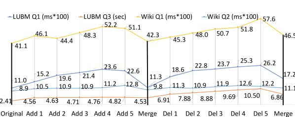
Figure 4 shows the runtime of four SPARQL queries after we added five new sets of triples to the KG, merged them, removed five other sets of triples, and merged again. Each set of added triples does not contain triples contained in previous updates. Similarly, each set of removed triples contains only triples in the original KG and not in previous updates. We selected the queries so that the content of the updates is considered. We observe that the runtime increases (because more deltas are considered) and that it drops after they are merged in a single update. Figure 5(a) reports the runtime to process five additions of ca. 1M novel triples, one merge, five removals of ca. 1M existing triples, and another merge. As we can see, with both datasets the runtime is much smaller than re-creating the database from scratch (>1h). The runtime with LUBM8k is faster than with Wikidata because the updates with the latter KG contained 4X more new entities.
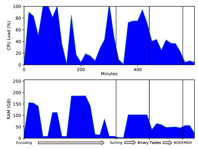
In Figure 5(b), we show the trace of the resource consumption during the loading of LUBM80k (10B triples). We plot the CPU (100% means all physical cores are used) and RAM usage. From it, we see that most of the runtime is taken to dictionary encoding, sorting the edges, and to create the binary tables.
In general, Trident has competitive loading times. Figure 5(c) shows the loading time of ours and other systems on LUBM1k. With larger KGs, RDF3X becomes significantly slower than ours (e.g., it takes ca. 7 hours to load LUBM8k on our smaller machine while Trident needs 1 hour and 18 minutes) due to lack of parallelism. TripleBit is an in-memory database and thus it cannot scale to some of our largest inputs. In some of our largest experiments, Trident could load LUBM400k (50B triples) in about 48 hours which is a size that other systems cannot handle. If the graph is already encoded, then loading is faster. We loaded the Hyperlink Graph (Meusel et al., 2015), a graph with 128B edges, in about 13 hours (with the larger machine) and the database required 1.4TB of space.
7. Related Work
In this section, we describe the most relevant works to our problem. For a broader introduction to graph and RDF processing, we redirect to existing surveys (McCune et al., 2015; Faye et al., 2011; Modoni et al., 2014; Sakr and Al-Naymat, 2010; Özsu, 2016; Abdelaziz et al., 2017a; Wylot et al., 2018). Current approaches can be classified either as native (i.e., designed for this task) or non-native (adapt pre-existing technology). Native engines have better performance (Bornea et al., 2013), but less functionalities (Bornea et al., 2013; Fan et al., 2015). Our approach belongs to the first category.
Research on native systems has focused on advanced indexing structures. The most popular approach is to extensively materialize a dedicated index for each permutation. This was initially proposed by YARS (Harth et al., 2007), and further explored in RDF3X (Baolin and Bo, 2007; Beckett, 2001; Fletcher and Beck, 2009; Bishop et al., 2011; Neumann and Weikum, 2010). Also Hexastore (Weiss et al., 2008) proposes a six-way permutation-based indexing, but implemented it using hierarchical in-memory Java hash maps. Instead, we use on-disk data structures and therefore can scale to larger inputs. Recently, other types of indices, based on 2D or 3D bit matrices (Atre et al., 2010; Yuan et al., 2013), hash-maps (Motik et al., 2014), or data structures used for graph matching approaches (Zou et al., 2014; Kim et al., 2015) have been proposed. If compared with these works, our approach uses a novel layout of data structures and uses multiple layouts to store the subgraphs.
Non-native approaches offload the indexing to external engines (mostly DBMS). Here, the challenge is to find efficient partitioning/replication criteria to exploit the multi-table nature of relational engines. Existing partitioning criteria group the triples either by predicates (Harris et al., 2009; Abadi et al., 2009; McBride, 2001; Ma et al., 2004; Neumann and Moerkotte, 2011; Pham et al., 2015; Pham and Boncz, 2016), clusters of predicates (Chong et al., 2005), or by using other entity-based splitting criteria (Bornea et al., 2013). The various partitioning schemes are designed to create few tables to meet the constraints of relational engines (Sidirourgos et al., 2008). Our approach differs because we group the edges at a much higher granularity generating a number of binary tables that is too large for such engines.
Some popular commercial systems for graph processing are Virtuoso (OpenLink Software, 2019), BlazeGraph (Systap, 2019), Titan (DATASTAX, Inc., 2019), Neo4J (Neo4j, Inc., 2019) Sparksee (Sparsity Technologies, 2019), and InfiniteGraph (Objectivity Inc., 2019). We compared Trident against such a leading commercial system and observed that ours has very competitive performance; other comparisons are presented in (Sidirourgos et al., 2008; Aluç et al., 2015). In general, a direct comparison is challenging because these systems provide end-to-end solutions tailored for specific tasks while we offer general-purpose low-level APIs.
Finally, many works have focused on distributed graph processing (Harris et al., 2009; Gurajada et al., 2014; Amann et al., 2018; Peng et al., 2016; Schätzle et al., 2016; Harbi et al., 2016; Lee and Liu, 2013; Zeng et al., 2013; Azzam et al., 2018; Abdelaziz et al., 2017b). We do not view these approaches as competitors since they operate on different hardware architectures. Instead, we view ours as a potential complement that can be employed by them to speed up distributed processing.
In our approach, we use numerical IDs to store the terms. This form of compression has been the subject of some studies. First, some systems use the Hash-code of the strings as IDs (Harris and Gibbins, 2003; Harris and Shadbolt, 2005; Harris et al., 2009). Most systems, however, use counters to assign new IDs (Broekstra et al., 2002; Harth and Decker, 2005; Harth et al., 2007; Neumann and Weikum, 2010; Martínez-Prieto et al., 2012a). It has been shown in (Urbani et al., 2016a) that assigning some IDs rather than others can improve the query answering due to data locality. It is straightforward to include these procedures in our system. Finally, some approaches focused on compressing RDF collections (Martínez-Prieto et al., 2012b) and on the management of the strings (Bazoobandi et al., 2015; Mavlyutov et al., 2015; Singh et al., 2018). We adopted a conventional approach to store such strings. Replacing our dictionary with these proposals is an interesting direction for future work.
8. Conclusion
We proposed a novel centralized architecture for the low-level storage of very large KGs which provides both node- and edge-centric access to the KG. One of the main novelties of our approach is that it exhaustively decomposes the storage of the KGs in many binary tables, serializing them in multiple byte streams to facilitate inter-table scanning, akin to permutation-based approaches. Another main novelty is that the storage effectively adapts to the KG by choosing a different layout for each table depending on the graph topology. Our empirical evaluation in multiple scenarios shows that our approach offers competitive performance and that it can load very large graphs without expensive hardware.
Future work is necessary to apply or adapt our architecture for additional scenarios. In particular, we believe that our system can be used to support Triple Pattern Fragments (Verborgh et al., 2016), an emerging paradigm to query RDF datasets, and GraphQL (Hartig and Pérez, 2018), a more complex graph query language. Finally, it is also interesting to study whether the integration of additional compression techniques, like locality-based dictionary encoding (Urbani et al., 2016a) or HDT (Fernández et al., 2013), can further improve the runtime and/or reduce the storage space.
Acknowledgments. We would like to thank (in alphabetical order) Peter Boncz, Martin Kersten, Stefan Manegold, and Gerhard Weikum for discussing and providing comments to improve this work. This project was partly funded by the NWO research programme 400.17.605 (VWData) and NWO VENI project 639.021.335.
Appendix A SPARQL queries
A.1. LUBM
PREFIX rdf: <http://www.w3.org/1999/02/
             22-rdf-syntax-ns#>
PREFIX ub:  <http://www.lehigh.edu/~zhp2/2004/
             0401/univ-bench.owl#>
Q1:
SELECT ?x WHERE {
?x ub:subOrganizationOf
   <http://www.Department0.University0.edu> .
?x rdf:type ub:ResearchGroup . }
Q2:
SELECT ?x WHERE {
?x ub:worksFor <http://www.Department0.University0.edu> .
?x rdf:type ub:FullProfessor . ?x ub:name ?y1 .
?x ub:emailAddress ?y2 . ?x ub:telephone ?y3 . }
Q3:
SELECT ?x ?y ?z WHERE {
?y rdf:type ub:University . ?z ub:subOrganizationOf ?y .
?z rdf:type ub:Department . ?x ub:memberOf ?z .
?x ub:undergraduateDegreeFrom ?y .
?x rdf:type ub:UndergraduateStudent. }
Q4:
SELECT ?x ?y ?z WHERE {
?y rdf:type ub:University . ?z ub:subOrganizationOf ?y .
?z rdf:type ub:Department . ?x ub:memberOf ?z .
?x rdf:type ub:GraduateStudent .
?x ub:undergraduateDegreeFrom ?y . }
Q5:
SELECT ?x ?y ?z WHERE {
?y rdf:type ub:FullProfessor . ?y ub:teacherOf ?z .
?z rdf:type ub:Course . ?x ub:advisor ?y .
?x ub:takesCourse ?z . }
A.2. DBPedia
PREFIX foaf: <http://xmlns.com/foaf/0.1/>
PREFIX dbo: <http://dbpedia.org/ontology/>
PREFIX db: <http://dbpedia.org/resource/>
PREFIX purl: <http://purl.org/dc/terms/>
PREFIX rdfs: <http://www.w3.org/2000/01/rdf-schema#>
Q1:
SELECT ?manufacturer ?name ?car
WHERE {
?car purl:subject db:Category:Luxury_vehicles .
?car foaf:name ?name .
?car dbo:manufacturer ?man .
?man foaf:name ?manufacturer . }
Q2:
SELECT ?film WHERE {
?film purl:subject db:Category:French_films . }
Q3:
SELECT ?title WHERE {
?game purl:subject db:Category:First-person_shooters .
?game foaf:name ?title . }
Q4:
SELECT ?name ?birth ?description ?person WHERE {
?person dbo:birthPlace db:Berlin .
?person purl:subject db:Category:German_musicians .
?person dbo:birthDate ?birth .
?person foaf:name ?name .
?person rdfs:comment ?description . }
Q5:
SELECT ?name ?birth ?death ?person WHERE {
?person dbo:birthPlace db:Berlin .
?person dbo:birthDate ?birth .
?person foaf:name ?name .
?person dbo:deathDate ?death .}
A.3. BTC2012
PREFIX geo: <http://www.geonames.org/ontology#>
PREFIX rdf: <http://www.w3.org/1999/02/
             22-rdf-syntax-ns#>
PREFIX dbpedia: <http://dbpedia.org/property/>
PREFIX dbpediares: <http://dbpedia.org/resource/>
PREFIX pos: <http://www.w3.org/2003/01/geo/wgs84_pos#>
PREFIX owl: <http://www.w3.org/2002/07/owl#>
Q1:
SELECT ?lat ?long WHERE {
?a ?x "Bro-C’hall" .
?a geo:inCountry <http://www.geonames.org/countries/
                  #FR> .
?a pos:lat ?lat . ?a pos:long ?long . }
Q2:
SELECT ?t ?lat ?long WHERE {
?a dbpedia:region
   dbres:List_of_World_Heritage_Sites_in_Europe .
?a dbpedia:title ?t . ?a pos:lat ?lat .
?a pos:long ?long .
?a dbpedia:link <http://whc.unesco.org/en/list/728> . }
Q3:
SELECT ?d WHERE {
?a dbpedia:senators ?c . ?a dbpedia:name ?d .
?c dbpedia:profession dbpediares:Politician .
?a owl:sameAs ?b .
?b geo:inCountry <http://www.geonames.org/countries/
                  #US> .}
Q4:
SELECT ?a ?b ?lat ?long WHERE {
?a dbpedia:spouse ?b .
?a rdf:type <http://dbpedia.org/ontology/Person> .
?b rdf:type <http://dbpedia.org/ontology/Person> .
?a dbpedia:placeOfBirth ?c . ?b dbpedia:placeOfBirth ?c .
?c owl:sameAs ?c2 . ?c2 pos:lat ?lat .
?c2 pos:long ?long . }
Q5:
SELECT ?a ?y WHERE {
?a rdf:type
   <http://dbpedia.org/class/yago/Politician110451263> .
?a dbpedia:years ?y.
?a <http://xmlns.com/foaf/0.1/name> ?n.
?b ?bn ?n.
?b rdf:type <http://dbpedia.org/ontology/OfficeHolder> . }
A.4. Uniprot
PREFIX r: <http://www.w3.org/1999/02/22-rdf-syntax-ns#>
PREFIX rs: <http://www.w3.org/2000/01/rdf-schema#>
PREFIX u: <http://purl.uniprot.org/core/>
Q1:
SELECT ?a ?vo WHERE {
?a u:encodedBy ?vo .
?a rs:seeAlso <http://purl.uniprot.org/eggnog/COG0787> .
?a rs:seeAlso <http://purl.uniprot.org/pfam/PF00842>.
?a rs:seeAlso <http://purl.uniprot.org/prints/PR00992>. }
Q2:
SELECT ?a ?vo WHERE {
?a u:annotation ?vo .
?a rs:seeAlso <http://purl.uniprot.org/interpro/IPR000842> .
?a rs:seeAlso <http://purl.uniprot.org/geneid/945772> .
?a u:citation <http://purl.uniprot.org/citations/9298646> . }
Q3:
SELECT ?p ?a WHERE {
?p u:annotation ?a .
?p r:type u:Protein .
?a r:type u:Transmembrane_Annotation . }
Q4:
SELECT ?p ?a WHERE {
?p u:annotation ?a .
?p r:type u:Protein .
?p u:organism <http://purl.uniprot.org/taxonomy/9606> .
?a r:type core/Disease_Annotation> . }
Q5:
SELECT ?a ?b ?ab WHERE {
?b u:modified "2008-07-22"^^
              <http://www.w3.org/2001/XMLSchema#date> .
?b r:type u:Protein . ?a u:replaces ?ab .
?ab u:replacedBy ?b . }
A.5. Wikidata
PREFIX wd: <http://www.wikidata.org/entity/>
PREFIX wdt: <http://www.wikidata.org/prop/direct/>
Q1:
SELECT ?h ?cause WHERE {
?h wdt:P39 wd:Q11696 .
?h wdt:P509 ?cause . }
Q2:
SELECT ?cat WHERE {
?cat  wdt:P31 wd:Q146 . }
Q3:
select ?gender WHERE {
?human wdt:P31 wd:Q5 .
?human wdt:P21 ?gender .
?human wdt:P106 wd:Q901 . }
Q4:
SELECT ?u ?state WHERE {
?u wdt:P31 wd:Q3918 .
?u wdt:P131 ?state .
?state wdt:P31 wd:Q35657 . }
Q5:
SELECT ?u ?x  WHERE {
?u wdt:P31 ?x .
?u wdt:P569 ?date }
References
- (1)
- Abadi et al. (2006) Daniel Abadi, Samuel Madden, and Miguel Ferreira. 2006. Integrating Compression and Execution in Column-Oriented Database Systems. In Proceedings of the 2006 ACM SIGMOD International Conference on Management of Data (Chicago, IL, USA) (SIGMOD ’06). Association for Computing Machinery, New York, NY, USA, 671–682. https://doi.org/10.1145/1142473.1142548
- Abadi et al. (2009) Daniel J. Abadi, Adam Marcus, Samuel R. Madden, and Kate Hollenbach. 2009. SW-Store: a vertically partitioned DBMS for Semantic Web data management. The VLDB Journal 18, 2 (2009), 385–406.
- Abdelaziz et al. (2017a) Ibrahim Abdelaziz, Razen Harbi, Zuhair Khayyat, and Panos Kalnis. 2017a. A Survey and Experimental Comparison of Distributed SPARQL Engines for Very Large RDF Data. Proceedings of the VLDB Endowment 10, 13 (Sept. 2017), 2049–2060. https://doi.org/10.14778/3151106.3151109
- Abdelaziz et al. (2017b) I. Abdelaziz, R. Harbi, S. Salihoglu, and P. Kalnis. 2017b. Combining vertex-centric graph processing with SPARQL for large-scale RDF data analytics. IEEE Transactions on Parallel and Distributed Systems 28, 12 (Dec. 2017), 3374–3388.
- Aluç et al. (2015) Günes Aluç, M. Tamer Özsu, Khuzaima Daudjee, and Olaf Hartig. 2015. Executing queries over schemaless RDF databases. In 31st IEEE International Conference on Data Engineering, ICDE 2015, Seoul, South Korea, April 13-17, 2015. IEEE Computer Society, Seoul, South Korea, 807–818. https://doi.org/10.1109/ICDE.2015.7113335
- Amann et al. (2018) Bernd Amann, Olivier Curé, and Hubert Naacke. 2018. Distributed SPARQL Query Processing: a Case Study with Apache Spark. John Wiley & Sons, Ltd, Chapter 2, 21–55. https://doi.org/10.1002/9781119528227.ch2
- Antoniou et al. (2018) Grigoris Antoniou, Sotiris Batsakis, Raghava Mutharaju, Jeff Z. Pan, Guilin Qi, Ilias Tachmazidis, Jacopo Urbani, and Zhangquan Zhou. 2018. A survey of large-scale reasoning on the Web of data. The Knowledge Engineering Review 33 (2018), 1–43.
- Atre et al. (2010) Medha Atre, Vineet Chaoji, Mohammed J. Zaki, and James A. Hendler. 2010. Matrix "Bit" Loaded: A Scalable Lightweight Join Query Processor for RDF Data. In Proceedings of the 19th International Conference on World Wide Web (Raleigh, North Carolina, USA) (WWW ’10). Association for Computing Machinery, New York, NY, USA, 41–50. https://doi.org/10.1145/1772690.1772696
- Azzam et al. (2018) A. Azzam, S. Kirrane, and A. Polleres. 2018. Towards Making Distributed RDF Processing FLINKer. In 2018 4th International Conference on Big Data Innovations and Applications (Innovate-Data). IEEE Computer Society, Los Alamitos, CA, USA, 9–16. https://doi.org/10.1109/Innovate-Data.2018.00009
- Baolin and Bo (2007) Liu Baolin and Hu Bo. 2007. HPRD: A High Performance RDF Database. In IFIP International Conference on Network and Parallel Computing (Lecture Notes in Computer Science), Keqiu Li, Chris Jesshope, Hai Jin, and Jean-Luc Gaudiot (Eds.). Springer Berlin Heidelberg, Dalian, China, 364–374.
- Bazoobandi et al. (2015) Hamid R. Bazoobandi, Steven de Rooij, Jacopo Urbani, Annette ten Teije, Frank van Harmelen, and Henri Bal. 2015. A Compact In-memory Dictionary for RDF Data. In The Semantic Web. Latest Advances and New Domains. Springer-Verlag New York, Inc., Portoroz, Slovenia, 205–220.
- Beckett (2001) David Beckett. 2001. The Design and Implementation of the Redland RDF Application Framework. In Proceedings of the 10th International Conference on World Wide Web (Hong Kong) (WWW ’01). Association for Computing Machinery, New York, NY, USA, 449–456. https://doi.org/10.1145/371920.372099
- Bishop et al. (2011) Barry Bishop, Atanas Kiryakov, Damyan Ognyanoff, Ivan Peikov, Zdravko Tashev, and Ruslan Velkov. 2011. OWLIM: A family of scalable semantic repositories. Semantic Web 2, 1 (2011), 33–42.
- Bizer et al. (2009) Christian Bizer, Jens Lehmann, Georgi Kobilarov, Sören Auer, Christian Becker, Richard Cyganiak, and Sebastian Hellmann. 2009. DBpedia-A crystallization point for the Web of Data. Web Semantics: science, services and agents on the world wide web 7, 3 (2009), 154–165.
- Blanco et al. (2013) Roi Blanco, Berkant Barla Cambazoglu, Peter Mika, and Nicolas Torzec. 2013. Entity Recommendations in Web Search. In The Semantic Web – ISWC 2013. Springer Berlin Heidelberg, Berlin, Heidelberg, 33–48.
- Bordes et al. (2013) Antoine Bordes, Nicolas Usunier, Alberto Garcia-Duran, Jason Weston, and Oksana Yakhnenko. 2013. Translating Embeddings for Modeling Multi-relational Data. In Advances in Neural Information Processing Systems 26, C. J. C. Burges, L. Bottou, M. Welling, Z. Ghahramani, and K. Q. Weinberger (Eds.). Curran Associates, Inc., Lake Tahoe, Nevada, USA, 2787–2795.
- Bornea et al. (2013) Mihaela A. Bornea, Julian Dolby, Anastasios Kementsietsidis, Kavitha Srinivas, Patrick Dantressangle, Octavian Udrea, and Bishwaranjan Bhattacharjee. 2013. Building an Efficient RDF Store over a Relational Database. In SIGMOD ’13: Proceedings of the 2013 ACM SIGMOD International Conference on Management of Data. ACM, New York, NY, USA, 121–132.
- Broekstra et al. (2002) Jeen Broekstra, Arjohn Kampman, and Frank Van Harmelen. 2002. Sesame: A Generic Architecture for Storing and Querying RDF and RDF Schema. In 1st International Semantic Web Conference. Springer, Sardinia, Italia, 54–68.
- Callahan et al. (2013) Alison Callahan, José Cruz-Toledo, Peter Ansell, and Michel Dumontier. 2013. Bio2RDF Release 2: Improved Coverage, Interoperability and Provenance of Life Science Linked Data. In 10th Extended Semantic Web Conference. Springer, Montperlier, France, 200–212.
- Ching et al. (2015) Avery Ching, Sergey Edunov, Maja Kabiljo, Dionysios Logothetis, and Sambavi Muthukrishnan. 2015. One Trillion Edges: Graph Processing at Facebook-Scale. Proceedings of the VLDB Endowment 8, 12 (Aug. 2015), 1804–1815. https://doi.org/10.14778/2824032.2824077
- Chong et al. (2005) Eugene Inseok Chong, Souripriya Das, George Eadon, and Jagannathan Srinivasan. 2005. An Efficient SQL-Based RDF Querying Scheme. In Proceedings of the 31st International Conference on Very Large Data Bases (VLDB ’05). VLDB Endowment, Trondheim, Norway, 1216–1227.
- DATASTAX, Inc. (2019) DATASTAX, Inc. 2019. Titan: Distributed Graph Database. http://titan.thinkaurelius.com/
- Fan et al. (2015) Jing Fan, Adalbert Gerald Soosai Raj, and Jignesh M. Patel. 2015. The Case Against Specialized Graph Analytics Engines.. In The 7th Biennial Conference on Innovative Data Systems Research CIDR 2015. www.cidrdb.org, Asilomar, California, USA.
- Faye et al. (2011) David C. Faye, Olivier Curé, and Guillaume Blin. 2011. A survey of RDF storage approaches. Revue Africaine de la Recherche en Informatique et Mathématiques Appliquées 15 (2011), 11–35.
- Fernández et al. (2013) Javier D. Fernández, Miguel A. Martínez-Prieto, Claudio Gutiérrez, Axel Polleres, and Mario Arias. 2013. Binary RDF representation for publication and exchange (HDT). Journal of Web Semantics 19 (March 2013), 22–41.
- Fletcher and Beck (2009) George H.L. Fletcher and Peter W. Beck. 2009. Scalable Indexing of RDF Graphs for Efficient Join Processing. In Proceedings of the 18th ACM Conference on Information and Knowledge Management (Hong Kong) (CIKM ’09). Association for Computing Machinery, New York, NY, USA, 1513–1516. https://doi.org/10.1145/1645953.1646159
- Gonzalez et al. (2012) Joseph E. Gonzalez, Yucheng Low, Haijie Gu, Danny Bickson, and Carlos Guestrin. 2012. PowerGraph: Distributed Graph-Parallel Computation on Natural Graphs. In 10th USENIX Symposium on Operating Systems Design and Implementation (OSDI 12). USENIX, Hollywood, CA, 17–30.
- Gonzalez et al. (2014) Joseph E. Gonzalez, Reynold S. Xin, Ankur Dave, Daniel Crankshaw, Michael J. Franklin, and Ion Stoica. 2014. GraphX: Graph Processing in a Distributed Dataflow Framework. In 11th USENIX Symposium on Operating Systems Design and Implementation (OSDI 14). USENIX Association, Broomfield, CO, 599–613.
- Gray (1981) Jim Gray. 1981. The Transaction Concept: Virtues and Limitations (Invited Paper). In Very Large Data Bases, 7th International Conference, September 9-11, 1981, Cannes, France, Proceedings. VLDB Endowment, Cannes, France, 144–154.
- Greaves and Mika (2008) Mark Greaves and Peter Mika. 2008. Semantic Web and Web 2.0. Web Semantics: Science, Services and Agents on the World Wide Web 6, 1 (2008), 1–3.
- Guha et al. (2003) R. Guha, Rob McCool, and Eric Miller. 2003. Semantic Search. In Proceedings of the 12th International Conference on World Wide Web (Budapest, Hungary) (WWW ’03). Association for Computing Machinery, New York, NY, USA, 700–709. https://doi.org/10.1145/775152.775250
- Guo et al. (2005) Yuanbo Guo, Zhengxiang Pan, and Jeff Heflin. 2005. LUBM: A benchmark for OWL knowledge base systems. Web Semantics: Science, Services and Agents on the World Wide Web 3, 2 (2005), 158–182.
- Gurajada et al. (2014) Sairam Gurajada, Stephan Seufert, Iris Miliaraki, and Martin Theobald. 2014. TriAD: A Distributed Shared-Nothing RDF Engine Based on Asynchronous Message Passing. In Proceedings of the 2014 ACM SIGMOD International Conference on Management of Data (Snowbird, Utah, USA) (SIGMOD ’14). Association for Computing Machinery, New York, NY, USA, 289–300. https://doi.org/10.1145/2588555.2610511
- Han et al. (2014) Minyang Han, Khuzaima Daudjee, Khaled Ammar, M. Tamer Özsu, Xingfang Wang, and Tianqi Jin. 2014. An Experimental Comparison of Pregel-like Graph Processing Systems. Proceedings of the VLDB Endowment 7, 12 (2014), 1047–1058. https://doi.org/10.14778/2732977.2732980
- Han et al. (2018) Xu Han, Shulin Cao, Xin Lv, Yankai Lin, Zhiyuan Liu, Maosong Sun, and Juanzi Li. 2018. OpenKE: An Open Toolkit for Knowledge Embedding. In Proceedings of the 2018 Conference on Empirical Methods in Natural Language Processing, EMNLP 2018: System Demonstrations, Brussels, Belgium, October 31 - November 4, 2018. Association for Computational Linguistics, Brussels, Belgium, 139–144.
- Harbi et al. (2016) Razen Harbi, Ibrahim Abdelaziz, Panos Kalnis, Nikos Mamoulis, Yasser Ebrahim, and Majed Sahli. 2016. Accelerating SPARQL queries by exploiting hash-based locality and adaptive partitioning. The VLDB Journal 25, 3 (2016), 355–380.
- Harris and Gibbins (2003) Stephen Harris and Nicholas Gibbins. 2003. 3store: Efficient Bulk RDF Storage. In 1st International Workshop on Practical and Scalable Semantic Systems (PSSS’03). ePrints Soton, Sanibel Island, FL, USA, 1–15.
- Harris et al. (2009) Steve Harris, Nick Lamb, and Nigel Shadbolt. 2009. 4store: The Design and Implementation of a Clustered RDF Store. In 5th International Workshop on Scalable Semantic Web Knowledge Base Systems (SSWS2009). CEUR Workshop Proceedings, Washington, DC, USA, 94–109.
- Harris et al. (2013) Steve Harris, Andy Seaborne, and Eric Prud’hommeaux. 2013. SPARQL 1.1 Query Language. http://www.w3.org/TR/sparql11-query
- Harris and Shadbolt (2005) Stephen Harris and Nigel Shadbolt. 2005. SPARQL query processing with conventional relational database systems. In International Conference on Web Information Systems Engineering. Springer, New York, NY, USA, 235–244.
- Harth (2012) Andreas Harth. 2012. Billion Triples Challenge data set. http://km.aifb.kit.edu/projects/btc-2012/
- Harth and Decker (2005) Andreas Harth and Stefan Decker. 2005. Optimized Index Structures for Querying RDF from the Web. In Proceedings of the Third Latin American Web Congress (LA-WEB ’05). IEEE Computer Society, Washington, DC, USA, 71–80.
- Harth et al. (2007) Andreas Harth, Jürgen Umbrich, Aidan Hogan, and Stefan Decker. 2007. YARS2: A Federated Repository for Querying Graph Structured Data from the Web. In The 6th International Semantic Web Conference (Lecture Notes in Computer Science). Springer Berlin Heidelberg, Busan, South Korea, 211–224.
- Hartig and Pérez (2018) Olaf Hartig and Jorge Pérez. 2018. Semantics and Complexity of GraphQL. In Proceedings of the 2018 World Wide Web Conference (Lyon, France) (WWW ’18). International World Wide Web Conferences Steering Committee, Republic and Canton of Geneva, CHE, 1155–1164. https://doi.org/10.1145/3178876.3186014
- Hayes (2004) Patrick Hayes. 2004. RDF Semantics, W3C Recommendation. http://www.w3.org/TR/rdf-mt/
- Kasneci et al. (2008) Gjergji Kasneci, Fabian M. Suchanek, Georgiana Ifrim, Maya Ramanath, and Gerhard Weikum. 2008. NAGA: Searching and Ranking Knowledge. In 24th International Conference on Data Engineering (ICDE). IEEE, Cancun, Mexico, 953–962.
- Kim et al. (2015) Jinha Kim, Hyungyu Shin, Wook-Shin Han, Sungpack Hong, and Hassan Chafi. 2015. Taming Subgraph Isomorphism for RDF Query Processing. Proceedings of the VLDB Endowment 8, 11 (2015), 1238–1249.
- Lee and Liu (2013) Kisung Lee and Ling Liu. 2013. Scaling queries over big RDF graphs with semantic hash partitioning. Proceedings of the VLDB Endowment 6, 14 (2013), 1894–1905.
- Leskovec and Krevl (2014) Jure Leskovec and Andrej Krevl. 2014. SNAP Datasets: Stanford Large Network Dataset Collection. http://snap.stanford.edu/data.
- Leskovec and Sosič (2016) Jure Leskovec and Rok Sosič. 2016. Snap: A general-purpose network analysis and graph-mining library. ACM Transactions on Intelligent Systems and Technology (TIST) 8, 1 (2016), 1.
- Ma et al. (2004) Li Ma, Zhong Su, Yue Pan, Li Zhang, and Tao Liu. 2004. RStar: An RDF Storage and Query System for Enterprise Resource Management. In Proceedings of the Thirteenth ACM International Conference on Information and Knowledge Management (Washington, D.C., USA) (CIKM ’04). Association for Computing Machinery, New York, NY, USA, 484–491. https://doi.org/10.1145/1031171.1031264
- Malewicz et al. (2010) Grzegorz Malewicz, Matthew H. Austern, Aart J.C Bik, James C. Dehnert, Ilan Horn, Naty Leiser, and Grzegorz Czajkowski. 2010. Pregel: A System for Large-Scale Graph Processing. In Proceedings of the 2010 ACM SIGMOD International Conference on Management of Data (Indianapolis, Indiana, USA) (SIGMOD ’10). Association for Computing Machinery, New York, NY, USA, 135–146. https://doi.org/10.1145/1807167.1807184
- Martínez-Prieto et al. (2012a) Miguel A. Martínez-Prieto, Javier D. Fernández, and Rodrigo Cánovas. 2012a. Compression of RDF Dictionaries. In Proceedings of the 27th Annual ACM Symposium on Applied Computing. ACM, Trento, Italy, 340–347.
- Martínez-Prieto et al. (2012b) Miguel A. Martínez-Prieto, Javier D. Fernández, and Rodrigo Cánovas. 2012b. Querying RDF dictionaries in compressed space. SIGAPP Appl. Comput. Rev. 12, 2 (June 2012), 64–77.
- Mavlyutov et al. (2015) Ruslan Mavlyutov, Marcin Wylot, and Philippe Cudre-Mauroux. 2015. A Comparison of Data Structures to Manage URIs on the Web of Data. In The Semantic Web. Latest Advances and New Domains. Springer-Verlag New York, Inc., Portoroz, Slovenia, 137–151.
- McBride (2001) Brian McBride. 2001. Jena: Implementing the RDF Model and Syntax Specification. In SemWeb’01 Proceedings of the Second International Conference on Semantic Web-Volume 40. CEUR-WS. org, Hong Kong, 23–28.
- McCune et al. (2015) Robert Ryan McCune, Tim Weninger, and Greg Madey. 2015. Thinking like a vertex: a survey of vertex-centric frameworks for large-scale distributed graph processing. ACM Computing Surveys (CSUR) 48, 2 (2015), 25.
- Meusel et al. (2015) Robert Meusel, Sebastiano Vigna, Oliver Lehmberg, and Christian Bizer. 2015. The Graph Structure in the Web – Analyzed on Different Aggregation Levels. The Journal of Web Science 1, 1 (2015), 33–47.
- Modoni et al. (2014) G. E. Modoni, M. Sacco, and W. Terkaj. 2014. A Survey of RDF Store Solutions. In 2014 International Conference on Engineering, Technology and Innovation (ICE). IEEE, Bergamo, Italy, 1–7.
- Motik et al. (2014) Boris Motik, Yavor Nenov, Robert Piro, Ian Horrocks, and Dan Olteanu. 2014. Parallel Materialisation of Datalog Programs in Centralised, Main-Memory RDF Systems. In Proceedings of the Twenty-Eighth AAAI Conference on Artificial Intelligence, July 27 -31, 2014, Québec City, Québec, Canada. AAAI Press, Québec, Canada, 129–137.
- Neo4j, Inc. (2019) Neo4j, Inc. 2019. Neo4j Graph Platform. https://neo4j.com/
- Neumann and Moerkotte (2011) Thomas Neumann and Guido Moerkotte. 2011. Characteristic sets: Accurate Cardinality Estimation for RDF Queries with Multiple Joins. In 27th International Conference on Data Engineering (ICDE). IEEE, Hannover, Germany, 984–994.
- Neumann and Weikum (2010) Thomas Neumann and Gerhard Weikum. 2010. The RDF-3X engine for scalable management of RDF data. The VLDB Journal 19, 1 (2010), 91–113.
- Nickel et al. (2015) Maximilian Nickel, Kevin Murphy, Volker Tresp, and Evgeniy Gabrilovich. 2015. A review of relational machine learning for knowledge graphs. Proc. IEEE 104, 1 (2015), 11–33.
- Noy et al. (2009) Natalya F. Noy, Nigam H. Shah, Patricia L. Whetzel, Benjamin Dai, Michael Dorf, Nicholas Griffith, Clement Jonquet, Daniel L. Rubin, Margaret-Anne Storey, and Christopher G. Chute. 2009. BioPortal: ontologies and integrated data resources at the click of a mouse. Nucleic acids research 37, suppl_2 (2009), W170–W173.
- Objectivity Inc. (2019) Objectivity Inc. 2019. InfiniteGraph. https://www.objectivity.com/products/infinitegraph/
- OpenLink Software (2019) OpenLink Software. 2019. Virtuoso RDF Engine. https://virtuoso.openlinksw.com/
- Özsu (2016) M. Tamer Özsu. 2016. A survey of RDF data management systems. Frontiers of Computer Science 10, 3 (2016), 418–432.
- Pal and Urbani (2017) Soumajit Pal and Jacopo Urbani. 2017. Enhancing Knowledge Graph Completion By Embedding Correlations. In Proceedings of the 2017 ACM on Conference on Information and Knowledge Management, CIKM 2017, Singapore, November 06 - 10, 2017. ACM, New York, NY, USA, 2247–2250.
- Peng et al. (2016) Peng Peng, Lei Zou, M. Tamer Özsu, Lei Chen, and Dongyan Zhao. 2016. Processing SPARQL queries over distributed RDF graphs. The VLDB Journal 25, 2 (2016), 243–268.
- Perez et al. (2015) Yonathan Perez, Rok Sosič, Arijit Banerjee, Rohan Puttagunta, Martin Raison, Pararth Shah, and Jure Leskovec. 2015. Ringo: Interactive Graph Analytics on Big-Memory Machines. In Proceedings of the 2015 ACM SIGMOD International Conference on Management of Data (Melbourne, Victoria, Australia) (SIGMOD ’15). Association for Computing Machinery, New York, NY, USA, 1105–1110. https://doi.org/10.1145/2723372.2735369
- Pham and Boncz (2016) Minh-Duc Pham and Peter Boncz. 2016. Exploiting Emergent Schemas to Make RDF Systems More Efficient. In The 15th International Semantic Web Conference – ISWC 2016 (Lecture Notes in Computer Science). Springer International Publishing, Kobe, Japan, 463–479.
- Pham et al. (2015) Minh-Duc Pham, Linnea Passing, Orri Erling, and Peter Boncz. 2015. Deriving an Emergent Relational Schema from RDF Data. In Proceedings of the 24th International Conference on World Wide Web (WWW ’15). International World Wide Web Conferences Steering Committee, Republic and Canton of Geneva, Switzerland, 864–874.
- Qin et al. (2014) Lu Qin, Jeffrey Xu Yu, Lijun Chang, Hong Cheng, Chengqi Zhang, and Xuemin Lin. 2014. Scalable Big Graph Processing in MapReduce. In Proceedings of the 2014 ACM SIGMOD International Conference on Management of Data (Snowbird, Utah, USA) (SIGMOD ’14). Association for Computing Machinery, New York, NY, USA, 827–838. https://doi.org/10.1145/2588555.2593661
- Redaschi and Consortium (2009) Nicole Redaschi and UniProt Consortium. 2009. UniProt in RDF: Tackling Data Integration and Distributed Annotation with the Semantic Web. Nature Precedings (2009).
- Rietveld and Hoekstra (2014) Laurens Rietveld and Rinke Hoekstra. 2014. YASGUI: Feeling the Pulse of Linked Data. In Knowledge Engineering and Knowledge Management - 19th International Conference, EKAW 2014, Linköping, Sweden, November 24-28, 2014. Proceedings (Lecture Notes in Computer Science). Springer International Publishing, Linköping, Sweden, 441–452.
- Sakr and Al-Naymat (2010) Sherif Sakr and Ghazi Al-Naymat. 2010. Relational Processing of RDF Queries: A Survey. SIGMOD Record 38, 4 (2010), 23–28. https://doi.org/10.1145/1815948.1815953
- Schätzle et al. (2016) Alexander Schätzle, Martin Przyjaciel-Zablocki, Simon Skilevic, and Georg Lausen. 2016. S2RDF: RDF Querying with SPARQL on Spark. Proceedings of the VLDB Endowment 9, 10 (2016), 804–815.
- Shao et al. (2013) Bin Shao, Haixun Wang, and Yatao Li. 2013. Trinity: A Distributed Graph Engine on a Memory Cloud. In Proceedings of the 2013 ACM SIGMOD International Conference on Management of Data (New York, New York, USA) (SIGMOD ’13). Association for Computing Machinery, New York, NY, USA, 505–516. https://doi.org/10.1145/2463676.2467799
- Shen et al. (2015) W. Shen, J. Wang, and J. Han. 2015. Entity linking with a knowledge base: issues, techniques, and solutions. IEEE Transactions on Knowledge and Data Engineering 27, 2 (2015), 443–460.
- Sidirourgos et al. (2008) Lefteris Sidirourgos, Romulo Goncalves, Martin Kersten, Niels Nes, and Stefan Manegold. 2008. Column-Store Support for RDF Data Management: not all swans are white. Proceedings of the VLDB Endowment 1, 2 (2008), 1553–1563.
- Singh et al. (2018) Gurkirat Singh, Dhawal Upadhyay, and Medha Atre. 2018. Efficient RDF Dictionaries with B+ Trees. In Proceedings of the ACM India Joint International Conference on Data Science and Management of Data (CoDS-COMAD ’18). ACM, New York, NY, USA, 128–136.
- Sparsity Technologies (2019) Sparsity Technologies. 2019. Sparksee. http://sparsity-technologies.com/
- Suchanek et al. (2008) Fabian M. Suchanek, Gjergji Kasneci, and Gerhard Weikum. 2008. YAGO: A Large Ontology from Wikipedia and WordNet. Web Semantics: Science, Services and Agents on the World Wide Web 6, 3 (2008), 203–217.
- Systap (2019) Systap. 2019. BlazeGraph. https://blazegraph.com/
- Tandon et al. (2014) Niket Tandon, Gerard de Melo, Fabian M. Suchanek, and Gerhard Weikum. 2014. WebChild: Harvesting and Organizing Commonsense Knowledge from the Web. In Seventh ACM International Conference on Web Search and Data Mining, WSDM 2014. ACM, New York, NY, USA, 523–532.
- Tonon et al. (2016) Alberto Tonon, Michele Catasta, Roman Prokofyev, Gianluca Demartini, Karl Aberer, and Philippe Cudre-Mauroux. 2016. Contextualized ranking of entity types based on knowledge graphs. Web Semantics: Science, Services and Agents on the World Wide Web 37 (2016), 170–183.
- Urbani et al. (2016a) Jacopo Urbani, Sourav Dutta, Sairam Gurajada, and Gerhard Weikum. 2016a. KOGNAC: Efficient Encoding of Large Knowledge Graphs. In Proceedings of the Twenty-Fifth International Joint Conference on Artificial Intelligence, IJCAI 2016, New York, NY, USA, 9-15 July 2016. AAAI Press, New York, NY, USA, 3896–3902.
- Urbani et al. (2016b) Jacopo Urbani, Ceriel Jacobs, and Markus Krötzsch. 2016b. Column-Oriented Datalog Materialization for Large Knowledge Graphs. In Proceedings of the Thirtieth AAAI Conference on Artificial Intelligence. AAAI Press, Phoenix, Arizona, USA, 258–264.
- Urbani et al. (2013) Jacopo Urbani, Jason Maassen, Niels Drost, Frank Seinstra, and Henri Bal. 2013. Scalable RDF data compression with MapReduce. Concurrency and Computation: Practice and Experience 25, 1 (2013), 24–39.
- Verborgh et al. (2016) Ruben Verborgh, Miel Vander Sande, Olaf Hartig, Joachim Van Herwegen, Laurens De Vocht, Ben De Meester, Gerald Haesendonck, and Pieter Colpaert. 2016. Triple Pattern Fragments: a low-cost knowledge graph interface for the Web. Web Semantics: Science, Services and Agents on the World Wide Web 37 (2016), 184–206.
- Vrandečić and Krötzsch (2014) Denny Vrandečić and Markus Krötzsch. 2014. Wikidata: a free collaborative knowledge base. Commun. ACM 57, 10 (2014), 78–85.
- Weiss et al. (2008) Cathrin Weiss, Panagiotis Karras, and Abraham Bernstein. 2008. Hexastore: sextuple indexing for semantic web data management. Proceedings of the VLDB Endowment 1, 1 (2008), 1008–1019.
- Williams and Zobel (1999) Hugh E. Williams and Justin Zobel. 1999. Compressing Integers for Fast File Access. Comput. J. 42, 3 (1999), 193–201. https://doi.org/10.1093/comjnl/42.3.193
- Wylot et al. (2018) Marcin Wylot, Manfred Hauswirth, Philippe Cudré-Mauroux, and Sherif Sakr. 2018. RDF Data Storage and Query Processing Schemes: A Survey. ACM Computing Surveys (CSUR) 51, 4 (2018), 84:1–84:36.
- Yahya et al. (2016) Mohamed Yahya, Denilson Barbosa, Klaus Berberich, Qiuyue Wang, and Gerhard Weikum. 2016. Relationship Queries on Extended Knowledge Graphs. In Proceedings of the Ninth ACM International Conference on Web Search and Data Mining (WSDM ’16). ACM, New York, NY, USA, 605–614.
- Yuan et al. (2013) Pingpeng Yuan, Pu Liu, Buwen Wu, Hai Jin, Wenya Zhang, and Ling Liu. 2013. TripleBit: a fast and compact system for large scale RDF data. Proceedings of the VLDB Endowment 6, 7 (2013), 517–528.
- Zeng et al. (2013) Kai Zeng, Jiacheng Yang, Haixun Wang, Bin Shao, and Zhongyuan Wang. 2013. A distributed graph engine for web scale RDF data. Proceedings of the VLDB Endowment 6, 4 (2013), 265–276.
- Zou et al. (2014) Lei Zou, M. Tamer Özsu, Lei Chen, Xuchuan Shen, Ruizhe Huang, and Dongyan Zhao. 2014. gStore: a graph-based SPARQL query engine. The VLDB Journal 23, 4 (2014), 565–590.