A multipolar effective one body waveform model for spin-aligned black hole binaries.

Abstract

We introduce TEOBiResumS_SM, an improved version of the effective-one-body (EOB) waveform model TEOBResumS for spin-aligned, coalescing black hole binaries, that includes subdominant gravitational waveform modes completed through merger and ringdown. Beyond the dominant $(\ell,|m|)=(2,2)$ one, the more robust multipoles all over the parameter space are: $(2,1)$, $(3,3)$, $(3,2)$, $(4,4)$ and $(5,5)$. Modes as $(3,1)$, $(4,3)$ and $(4,2)$ can also be generated, but are less robust. The multipolar ringdown EOB waveform stems from suitably fitting many numerical relativity (NR) waveform data from the Simulating eXtreme Spacetimes (SXS) collaboration together with test-mass waveform data. Mode-mixing effects are not incorporated. The orbital (nonspinning) part of the multipolar waveform amplitudes includes test-mass results up to (relative) 6PN order and, for most modes, is Padé resummed. The $m$=odd waveform multipoles (up to $\ell=5$) incorporate most of the currently available spin-dependent analytical information. Each multipolar amplitude is additionally orbital-factorized and resummed. Improving on previous work, we confirm that certain $m=\text{odd}$ modes, e.g. the $(2,1)$, and even the $(3,1)$, may develop a zero (or a minimum) in the amplitude for nearly equal-mass binaries and for several combinations of the individual spins. A remarkable EOB/NR agreement around such zero is found for these modes. The new waveform, and radiation reaction, prompts a new NR-calibration of the spinning sector of the model, done with only $32$ datasets. The maximum $(2,2)$ EOB/NR unfaithfulness $\bar{F}$ with Advanced LIGO noise against the SXS catalog ($\sim 595$ datasets) is always below $0.5\%$ for binaries with total mass $M$ as $10M_{\odot}\leq M\leq 200M_{\odot}$, except for a single outlier with $\max{(\bar{F})}\sim 0.85\%$. When $(2,1)$, $(3,3)$ and $(4,4)$ modes are included, one finds an excellent EOB/NR agreement up to $M\sim 120M_{\odot}$, above which the performance degrades slightly and moves above $3\%$ We also point out that the EOB dynamics may develop unphysical features for large, anti-aligned, spins and this may impact the correct construction of the $(2,1)$ mode in some corners of the parameter space.

I Introduction

The recent observation made by LIGO Aasi et al. (2015) and Virgo Acernese et al. (2015) of gravitational wave (GW) signals from twelve coalescing compact binaries marked the beginning of the era of gravitational wave astronomy. Of these detections, ten were associated to coalescing binary black holes (BBHs) Abbott et al. (2016a, b, 2017a, 2017b, 2017c, 2019) and two to a binary neutron star (BNS) Abbott et al. (2017d, 2020).

Up to recent times, gravitational waveform models used on LIGO and Virgo data only incorporated the dominant $(\ell=2,m=2)$ mode. This may be sufficient when the binary system is highly symmetric (e.g nearly equal masses and nearly equal spins), but for binaries when one object is more massive than the other, or when the spins are very different, modeling the subdominant multipoles becomes an absolute necessity to avoid potential biases in the parameters O’Shaughnessy et al. (2014); Varma and Ajith (2017). Similarly, at large inclinations, the modeling of gravitational wave modes beyond the dominant mode becomes increasingly important as higher modes are geometrically suppressed in the face-on/off limit. For this reason, there were recent efforts in building waveform models that incorporate the subdominant modes. This was the case for phenomenological models, both in the spinning London et al. (2018) or nonspinning case Mehta et al. (2017), or for effective-one-body (EOB) models Cotesta et al. (2018) for spin aligned black hole binaries. In addition, Ref. Varma et al. (2019) took advantage of a huge number of high-quality numerical relativity simulations from the SXS collaboration to construct a numerical relativity (NR) surrogate model with as many modes as possible (also including the $m=0$ ones).

Within the effective-one-body framework Buonanno and Damour (1999, 2000); Damour et al. (2000); Damour (2001); Damour et al. (2015) for coalescing black-hole binaries, the SEOBNRv4HM model introduced in Ref. Cotesta et al. (2018) is the higher-mode version of the SEOBNRv4 Bohé et al. (2017) spin-aligned model, calibrated to NR simulations, while SEOBNRv4HMP is its precessing version Ossokine et al. (2020) and represents current state of the art. Alternatively to SEOBNRv4, a different spin-aligned EOB model, informed by NR simulations, is TEOBResumS. This model was introduced in Nagar et al. (2018), and used to independently infer the parameters of GW150914 Abbott et al. (2016a). Although this waveform model is limited to the $\ell=m=2$ dominant mode, is publicly available either as a stand-alone $C$ code based on the GSL library or through the LIGO LALSuite LIGO Scientific Collaboration (2018) library. One of the advantages of this model is that it implements the description of the inspiral dynamics based on the (high-order) post-adiabatic (PA) approximation Nagar and Rettegno (2019); Akcay et al. (2019); Nagar et al. (2019a). This allows one to generate long-inspiral waveforms so efficiently to be of direct use for parameter estimation purposes (see also Ref. Rettegno et al. (2019) where the same approach is applied to the SEOBNRv4 Hamiltonian).

Recently, in a companion paper Nagar et al. (2019b), hereafter Paper I, the nonspinning sector of TEOBResumS, was augmented with all subdominant waveform modes, completed through merger and ringdown, up to $\ell=m=5$ included. This defined the TEOBiResumMultipoles model. In doing so, the EOB orbital interaction potential was improved thanks to a more stringent comparison with state-of-the-art NR simulations with small uncertainties. This led us to construct a multipolar model with EOB/NR unfaithfulness at most of the order of $2\%$ (and typically well below $1\%$) for total mass up to $200M_{\odot}$ and mass ratio in the range $1\leq q\leq 10$. It was also possible to verify that the model performs excellently up to $q=18$, that is the NR dataset with the largest mass ratio currently available to us.

The purpose of the present work is to generalize the results of Paper I to the case of spin-aligned black-hole binaries. To improve the robustness of the multipolar waveform amplitudes towards merger, we build upon Refs. Nagar and Shah (2016); Messina et al. (2018), implementing the corresponding orbital factorization and resummation paradigm, though limited to the $m=$odd waveform modes. Together with the changes in the nonspinning part of the dynamics discussed in Paper I, this led us to a new determination of the next-to-next-to-next-to-leading (NNNLO) spin-orbit effective parameter $c_{3}$ introduced long ago Damour and Nagar (2014a); Nagar et al. (2016). The construction of the multipolar waveform around the amplitude peak of each multipole (e.g. around merger), of the next-to-quasi-circular (NQC) corrections and of the postpeak-ringdown phase follows the procedure discussed, multipole by multipole, for the nonspinning case in Paper I. The only difference is that some of the NR-informed fits incorporate now a suitable spin-dependence. The reader should be aware that this paper stems from Refs. Damour and Nagar (2014a, b); Nagar et al. (2016); Nagar and Shah (2016); Del Pozzo and Nagar (2017); Nagar et al. (2017, 2018) and it is essentially the follow up of Refs. Nagar et al. (2018, 2019b). As such, it adopts the same notations and conventions. For this reason, we shall assume the reader to be familiar with the notation and language of those papers, that might not be reintroduced if not absolutely necessary.

The paper is organized as follows. In Sec. II we review the elements of the EOB dynamics that remained unchanged with respect to Nagar et al. (2018) and Paper I; we discuss the structure of the new multipolar waveform and the related new determination of $c_{3}$. Section III summarizes describes in details the numerical waveforms employed in this paper (either to inform the model or to check it), focusing in particular on an estimate of their uncertainty. Section IV probes the $(2,2)$ mode all over the current release of the SXS catalog Boyle et al. (2019). Section V focuses on the behavior of higher multipolar modes, highlighting several aspects related to their accurate modelization. In particular, it is pointed out, and explained, the peculiar behavior of some $m=1$ modes. The important EOB/NR unfaithfulness computations with higher modes are also performed there. Our concluding remarks are then collected in Sec. VI. The bulk of the text is complemented by several Appendixes. Appendix A discusses in detail the nonspinning limit of the model; Appendix B highlights a few systematics in the SXS waveform data that are relevant for higher modes; Appendix C reports all the NR-informed fits that are needed to accurately build the merger and ringdown part of the multipolar waveform.

If not otherwise specified, we use natural units with $c=G=1$. Our notations are as follows: we denote with $(m_{1},m_{2})$ the individual masses, while the mass ratio is $q\equiv m_{1}/m_{2}\geq 1$. The total mass and symmetric mass ratio are then $M\equiv m_{1}+m_{2}$ and $\nu=m_{1}m_{2}/M$. We also use the mass fractions $X_{1,2}\equiv m_{1,2}/M$ and $X_{12}\equiv X_{1}-X_{2}=\sqrt{1-4\nu}$. We address with $(S_{1},S_{2})$ the individual, dimensionful, spin components along the direction of the orbital angular momentum. The dimensionless spin variables are denoted as $\chi_{1,2}\equiv S_{1,2}/(m_{1,2})^{2}$. We also use $\tilde{a}_{1,2}\equiv X_{1,2}\chi_{1,2}$, the effective spin $\tilde{a}_{0}=\tilde{a}_{1}-\tilde{a}_{2}$ and $\tilde{a}_{12}\equiv\tilde{a}_{1}-\tilde{a}_{2}$.

Table 1: Resummation choices used to build our multipolar EOB waveform. The bar denotes resummation using the inverse Taylor expansion, as described by Eq. (5) of Ref. Nagar and Shah (2016). The PN-order should be intended relative to the leading-order term and also indicates the order of the additional (spinning) test-particle terms. For example, 3.5PN means that we take a polynomial of the form $1+x^{3/2}+x^{2}+x^{5/2}+...+x^{7/2}$, with the known $\nu$ dependence in the coefficients. Instead, $1.5^{+1}$PN means that we add to the $\nu$-dependent 1.5PN-accurate polynomial an additional term proportional to $x^{5/2}$ obtained by suitably incorporating spinning p article terms as illustrated in Sec. VB of Ref. Messina et al. (2018). We denote Padé resummation by $P^{n}_{d}$, where $N=n+d$ is the PN order.

$(\ell,m)$	Resummation choices		Relative PN order
	orbital	spin	orbital	spin
$(2,2)$	$P^{5}_{0}[\rho_{22}^{\rm orb}]$	$T[\rho_{22}^{\rm S}]$	$3^{+2}$PN	3.5PN without NNLO SO term
$(2,1)$	$P_{1}^{5}[\rho_{21}]$	$\hat{f}_{21}^{\rm S}=X_{12}\overline{\hat{f}^{\rm S_{(0)}}_{21}}-\dfrac{3}{2}\tilde{a}_{12}x^{1/2}\overline{\hat{f}_{21}^{\rm S_{(1)}}}$	$3^{+3}$PN	2.5PN
$(3,3)$	$P_{2}^{4}[\rho_{33}]$	$\hat{f}_{33}^{\rm S}=X_{12}\overline{\hat{f}^{\rm S_{(0)}}_{33}}+\left(-\dfrac{1}{4}+\dfrac{5}{2}\nu\right)\tilde{a}_{12}x^{3/2}\hat{f}_{33}^{\rm S_{(1)}}$	$3^{+3}$PN	2.5PN
$(3,2)$	$P^{4}_{2}[\rho_{32}]$	$T[\rho_{32}^{\rm S}]$	$2^{+2}$PN	$1.5^{+1}$PN (SO only)
$(3,1)$	$P_{2}^{3}[\rho_{31}^{\rm orb}]$	$\hat{f}_{31}^{\rm S}=X_{12}\overline{\hat{f}^{\rm S_{(0)}}_{31}}+\left(-\dfrac{9}{4}+\dfrac{13}{2}\nu\right)\tilde{a}_{12}x^{3/2}\hat{f}_{31}^{\rm S_{(1)}}$	$3^{+2}$PN	2.5PN
$(4,4)$	$P^{6}_{0}[\rho_{44}^{\rm orb}]$	$T[\rho_{44}^{\rm S}]$	$2^{+4}$PN	$1.5^{+2}$PN (SO only)
$(4,3)$	$P_{2}^{4}[\rho_{43}^{\rm orb}]$	$\hat{f}_{43}^{\rm S}=X_{12}\hat{f}^{\rm S_{(0)}}_{43}-\dfrac{5}{4}\tilde{a}_{12}x^{1/2}$	$1^{+5}$PN	0.5PN (SO only)
$(4,2)$	$P^{6}_{0}[\rho_{42}^{\rm orb}]$	$T[\rho_{42}^{\rm S}]$	$2^{+4}$PN	$1.5^{+3}$PN (SO only)
$(4,1)$	$P_{2}^{4}[\rho_{41}^{\rm orb}]$	$\hat{f}_{41}^{\rm S}=X_{12}\hat{f}^{\rm S_{(0)}}_{41}-\dfrac{5}{4}\tilde{a}_{12}x^{1/2}$	$1^{+5}$PN	0.5PN (SO only)
$(5,5)$	$P_{0}^{6}[\rho_{55}^{\rm orb}]$	$\hat{f}_{55}^{\rm S}=X_{12}\overline{\hat{f}_{55}^{{\rm S}_{(0)}}}+10\nu\dfrac{(1-3\nu)}{3-6\nu}\tilde{a}_{12}x^{3/2}$	$1^{+5}$PN	2PN

II The model: Relative dynamics and multipolar waveform

In this Section we collect the analytical elements of TEOBiResumS_SM that change with respect to the original implementation of TEOBResumS of Nagar et al. (2018) or that stem from results of Paper I. The modifications regard all building blocks of the model: the Hamiltonian, the inspiral, EOB-resummed, waveform as well as the merger-ringdown part. However, the structure of the Hamiltonian is precisely the same of TEOBResumS: there is thus no need to describe it here in detail and we address the reader to Sec. II of Ref. Nagar et al. (2018). The modifications are limited to the NR-informed effective 5PN coefficient $a_{6}^{c}(\nu)$ (that coincides with the function determined in Paper I) as well as the effective NNNLO spin-orbit parameter $c_{3}(\nu,\tilde{a}_{1},\tilde{a}_{2})$. This one needs to be redetermined, by phasing comparison with NR simulations, because of both the new $a_{6}^{c}(\nu)$, that has changed with respect to Ref. Nagar et al. (2018), and the new analytical choice for the factorized (and resummed) multipolar waveform taken from Ref. Messina et al. (2018). In addition, we also present here a new, spin-dependent, description of the multipolar merger and ringdown waveform, that is based on fits informed by NR simulations. These fits incorporate some, but not all, spin dependence for all modes up to $\ell=m=5$, as we detail in Appendix C. We start by discussing the structure of the resummed waveform.

II.1 Inspiral multipolar waveform

The waveform amplitudes we use here incorporate several factorization and resummation procedures that have been discussed in previous literature Damour et al. (2009); Pan et al. (2011); Nagar and Shah (2016); Messina et al. (2018). One should be warned that there are not ubiquitous recipes for what concerns the choice of resummation and/or the multipolar order to use: each multipolar amplitude can, in principle, be treated separately from the others. In practice, following Paper I, we attempt to comply at the idea of using 6PN-accurate hybrid orbital (i.e. nonspinning) amplitudes that are, whenever possible, resummed using Padé approximants. By “hybrid” we mean that the $\nu$-dependent terms, analytically known up to 3PN accuracy, are augmented by test-particle terms up to getting a relative 6PN order in all the residual waveform amplitudes. The spin sector takes advantage of some of, but not all, the new PN information at next-to-next-to-leading-order (NNLO) that was recently presented in Ref. Cotesta et al. (2018) adapting (yet unpublished) results of S. Marsat and A. Bohé. Practically all the structure of the waveform was discussed in Sec. IIIB, IIIC and IIID and of Paper I. Since we are adopting the same notation and nomenclature introduced there, it is not worth to repeat it here. We only recall that the acronym NQC stands for “next-to-quasi-circular” and that $f_{\ell m}$’s or $\rho_{\ell m}\equiv(f_{\ell m})^{1/\ell}$ functions are the residual waveform amplitudes. For resumming the $m=\text{odd}$ mode waveform amplitudes we implement the orbital-factorization and resummation scheme of Ref. Messina et al. (2018). In brief, following the notation of this latter reference, our analytical choices for the waveform amplitudes are listed in Table 1. We give below more details, discussing explicitly, and separately, the orbital and spin sectors.

II.1.1 Orbital sector

All $\nu$-dependent terms in the multipolar amplitudes up to $\ell=6$ are augmented with test-particle terms up to relative (hybrid) order 6PN except for the $(2,2)$ and $(3,1)$ modes, that rely on $3^{+2}$ PN information, consistently with previous work. For most of the modes, such 6PN-accurate, hybridized, amplitudes are additionally Padé resummed consistently with the choice made in the extreme-mass-ratio limit in Ref. Messina et al. (2018). Note however that some multipoles actually behave better (when compared with test-mass numerical data) when they are left in nonresummed form. Table 1 lists, in the second column, the analytical representation chosen for the orbital factors up to $\ell=m=5$. We address the Padé approximant of order $(n,d)$ with the usual notation $P^{n}_{d}$, where $n$ is the polynomial order of the numerator and $d$ the one of the denominator. For notational consistency, we also indicate with $P^{n}_{0}$ the Taylor-expanded form of the functions. The subdominant modes that do not contain spin information are not reported in the table. The $(5,1)$, $(6,1)$, $\ell=7$ and $\ell=8$ modes are kept in Taylor-expanded form at (global) $3^{+2}$ PN order for simplicity, consistently with previous work. All other $\rho_{\ell m}^{\rm orb}$’s with $\ell=5$ and $\ell=6$ are resummed as $P^{4}_{2}\left(\rho_{\ell m}^{\rm orb}\right)$ approximants.

II.1.2 Spin sector

The spin-dependent terms in the waveform amplitudes are incorporated only in those multipoles where the $\nu$-dependence beyond the leading order is analytically known, i.e. up to $\ell=m=5$, as illustrated in Table 1. For some modes, the $\nu$-dependent information is augmented with spinning-particle terms, according to the hybridization procedure discussed in Ref. Messina et al. (2018). Note that the analytical resummation of the residual waveform amplitudes to improve their robustness in the strong-field, fast-velocity regime when $m=\text{even}$ is not the same as when $m=\text{odd}$. For the $m=\text{even}$ modes, the residual amplitudes are written as

$$P^{n}_{d}\left[\rho^{\rm orb}_{\ell m}\right]+\rho_{\ell m}^{\rm S},$$ (1)

where we explicitly indicate the fact that the orbital part is Padé resummed (including in this nomenclature also the plain Taylor-expansion) according to Table 1. By contrast, the spin-dependent part is kept in Taylor-expanded form, with the (relative) PN order given in Table 1. Here, the notation $T[\rho_{{\ell m}}^{\rm S}]$ is an explicit reminder that we are using the $\rho_{\ell m}^{\rm S}$ in Taylor-expanded form. The amount of analytical information used in each mode is listed in the fifth column of the table. First of all, note that we do not include the NNLO spin-orbit term in $\rho_{22}^{\rm S}$ that was recently computed and is part of either SEOBNRv4 Bohé et al. (2017) and SEOBNRv4HM Cotesta et al. (2018). As it was pointed out already in Ref. Nagar and Shah (2016), this term has a large impact on the EOB waveform towards merger for large, positive, spins, so that the EOB/NR difference is larger with this term than without it (see Fig. 6 of Nagar and Shah (2016)). By contrast, the NLO-accurate amplitude alone already delivers an excellent representation of the corresponding NR amplitude and thus gives a more robust starting point for the action of the NQC factor. We do, however, include the LO cubic-in-spin term in $\rho_{22}^{\rm S}$. Browsing the fifth column of Table 1 the notation adopted indicates that the $\nu$-dependent terms in $(\rho_{32}^{\rm S},\rho_{44}^{\rm S},\rho_{42}^{\rm S})$ were hybridized with some of the higher-order, spin-orbit, terms obtained in the limit of a spinning particle on a Schwarzschild black hole in Ref. Nagar et al. (2019c). The rational behind such hybridization procedure is discussed in Sec. VB of Ref. Messina et al. (2018) and allows one to incorporate some of the leading-in-$\nu$-dependence by suitably “dressing” the $\nu=0$ information. One finds that the additional terms are such to increase the EOB/NR waveform ampltiude agreement towards merger in a natural way. To be explicit, we have

$$\rho_{32}^{\rm S}=c^{{\rm SO}_{\rm lo}}x^{1/2}+c^{\rm SO_{\rm nlo}}_{32}x^{3/2}+c^{{\rm SO}_{\rm nnlo}}_{32}x^{5/2},$$ (2)

where $(c^{{\rm SO}_{\rm lo}},c^{{\rm SO}_{\rm nlo}})$ are the usual known terms with the full $\nu$ dependence (see e.g. Messina et al. (2018) for their explicit form), while

$$c^{{\rm SO}_{\rm nnlo}}_{32}=-\dfrac{2571199}{1924560}\tilde{a}_{0}-\dfrac{1844993}{1924560}\tilde{a}_{12}X_{12},$$ (3)

that reduces to the known spinning test-particle terms when $\nu\to 0$. Similarly, $\rho_{44}^{\rm S}$ reads

$$\rho_{44}^{\rm S}=c^{\rm SO_{\rm lo}}_{44}x^{3/2}+c^{\rm SO_{\rm nlo}}_{44}x^{5/2}+c^{\rm SO_{\rm nnlo}}_{44}x^{7/2},$$ (4)

where

$$c^{\rm SO_{\rm nlo}}_{44} =-\dfrac{199}{550}\tilde{a}_{0}-\dfrac{491}{550}\tilde{a}_{12}X_{12},$$ (5)

$$c^{\rm SO_{\rm nnlo}}_{44} =\dfrac{527001653}{264264000}\tilde{a}_{0}+\dfrac{3208967}{264264000}\tilde{a}_{12}X_{12},$$ (6)

For $\rho_{42}^{\rm S}$ we have

$$\rho_{42}^{\rm S}=c^{\rm SO_{\rm lo}}_{42}x^{3/2}+c^{\rm SO_{\rm nlo}}_{42}x^{5/2}+c^{\rm SO_{\rm nnlo}}_{42}x^{7/2}+c^{\rm SO_{\rm nnnlo}}_{42}x^{9/2},$$ (7)

where the $\nu$-dressed spinning particle coefficients read

$$c^{\rm SO_{\rm nlo}}_{42} =-\dfrac{219}{550}\tilde{a}_{0}+\dfrac{92}{275}\tilde{a}_{12}X_{12},$$ (8)

$$c^{\rm SO_{\rm nnlo}}_{42} =-\dfrac{329051729}{264264000}\tilde{a}_{0}+\dfrac{169512229}{264264000}\tilde{a}_{12}X_{12},$$ (9)

$$c^{\rm SO_{\rm nnnlo}}_{42} =-\left(\dfrac{32079746680643}{16482145680000}+\dfrac{17581}{51975}{\rm eulerlog}(x,2)\right)\tilde{a}_{0}$$

$$\!\!\!\!\!\!\!\!\!\!\!\!-\left(\dfrac{28943192016227}{16482145680000}-\dfrac{10697}{51975}{\rm eulerlog}(x,2)\right)\tilde{a}_{12}X_{12}.$$ (10)

For the $m=\text{odd}$ modes, we apply in full the factorization of the orbital term and subsequent resummation of the spin factor with its inverse Taylor representation as illustrated in Ref. Messina et al. (2018). Recalling the notation therein, each $m$-odd waveform mode is written as

$$h_{\ell m}^{(\epsilon)}=h_{\ell m}^{N,(\epsilon)^{\prime}}\tilde{h}^{(\epsilon)}_{\ell m},$$ (11)

where $h_{\ell m}^{N,(\epsilon)^{\prime}}$ is the usual Newtonian prefactor Damour et al. (2009) with the overall factor $X_{12}$ factorized out, while

$$\tilde{h}^{(\epsilon)}_{\ell m}\equiv X_{12}\hat{h}^{(\epsilon)}_{\ell m},$$ (12)

and $\hat{h}^{(\epsilon)}_{\ell m}$ is the usual relativistic correction Damour et al. (2009). The $m$-odd relativistic waveform correction is then factorized as

$$\tilde{h}^{(\epsilon)}_{\ell m}=\hat{S}^{(\epsilon)}_{\rm eff}\hat{h}_{\ell m}^{\rm tail}e^{{\rm i}\delta_{\ell m}}\left[P^{n}_{d}\left(\rho_{\ell m}^{\rm orb}\right)\right]^{\ell}\hat{f}_{\ell m}^{\rm S},$$ (13)

where $(\hat{h}^{\rm tail}_{\ell m},\delta_{\ell m})$ are the usual, well known, tail factor and residual phase correction Damour et al. (2009). The spin-dependent $\hat{f}^{\rm S}_{\ell m}$ functions that we use are summarized in Table 1. The same table also lists the Padé approximants $P^{n}_{d}[\rho_{\ell m}^{\rm orb}]$ adopted for the orbital factors. For the spin factors, we take advantage of the new NNLO results of Ref. Cotesta et al. (2018), in particular those concerning the $\ell=m=5$ mode. This multipole is also resummed consistently with the others. In particular, it also includes the 2PN-accurate (or relative LO) spin-square term. The inverse-resummed factor $\overline{\hat{f}^{S_{(0)}}_{55}}$ explicitly reads

$$\overline{\hat{f}^{S_{(0)}}_{55}}=\left(1+\dfrac{10}{3}\tilde{a}_{0}x^{3/2}-\dfrac{5}{2}\tilde{a}_{0}^{2}x^{2}\right)^{-1}.$$ (14)

The global structure of the spin factors is illustrated in Table 1 and we do not discuss here any further as it is a straightforward application of the procedure of Ref. Messina et al. (2018) once modified with the new PN terms published in Ref. Cotesta et al. (2018) and the spinning-particle terms of Ref. Nagar et al. (2019c).

II.1.3 Residual phase corrections $\delta_{\ell m}$

Let us finally detail the expression of the $\delta_{\ell m}$ we use. Following Ref. Damour et al. (2013), we mostly use them in Padé resummed form, augmenting, for some modes, the 3.5PN, $\nu$-dependent terms with the next, 4.5PN-accurate, contribution in the test-particle limit Fujita (2015). In addition, we only rely on nonspinning information, although spin-dependent terms are available Cotesta et al. (2018). Explicitly, the expressions we use read

$$\delta_{22}= ~{}\frac{7}{3}y^{\frac{3}{2}}\frac{808920\nu\pi\sqrt{y}+137388\pi^{2}y+35\nu^{2}\left(136080+(154975-1359276\nu)y\right)}{808920\nu\pi\sqrt{y}+137388\pi^{2}y+35\nu^{2}\left(136080+(154975+40404\nu)y\right)},$$ (15)

$$\delta_{21}= ~{}\frac{2}{3}y^{\frac{3}{2}}\frac{5992\pi\sqrt{y}+2465\nu(28-493\nu y)}{69020\nu+5992\pi\sqrt{y}},$$ (16)

$$\delta_{33}= ~{}\frac{13}{10}y^{\frac{3}{2}}\frac{1+\frac{94770\pi}{566279\nu}\sqrt{y}}{1+\frac{94770\pi}{566279\nu}\sqrt{y}+\frac{80897}{3159}\nu y},$$ (17)

$$\delta_{32}= ~{}\frac{10+33\nu}{15(1-3\nu)}y^{\frac{3}{2}}\frac{1}{1-\frac{260(1-3\nu)}{7(10+33\nu)}\pi y^{\frac{3}{2}}+\frac{1}{(10+33\nu)^{2}}\left(\frac{91120}{27}+\frac{9112}{9}\nu-\frac{100232}{3}\nu^{2}+\frac{130000}{147}\pi^{2}-\frac{412880}{49}\nu\pi^{2}+\frac{848640}{49}\nu^{2}\pi^{2}\right)y^{3}},$$ (18)

$$\delta_{31}= ~{}\frac{13}{30}y^{\frac{3}{2}}\frac{4641\nu+1690\pi\sqrt{y}}{4641\nu+1690\pi\sqrt{y}+18207\nu^{2}y},$$ (19)

$$\delta_{44}= ~{}\frac{112+219\nu}{120(1-3\nu)}y^{\frac{3}{2}}\frac{1}{1-\frac{201088(1-3\nu)}{231(112+219\nu)}\pi y^{\frac{3}{2}}-\frac{1-3\nu}{(112+219\nu)^{2}}\left(\frac{49409024}{25}+\frac{96612288}{25}\nu+\frac{8854306816}{17787}\pi^{2}-\frac{49478908928}{17787}\nu\pi^{2}\right)y^{3}},$$ (20)

$$\delta_{43}= ~{}\frac{486+4961\nu}{810(1-2\nu)}y^{\frac{3}{2}}\Bigg{[}1-\frac{254502(1-2\nu)}{77(486+4961\nu)}\pi y^{\frac{3}{2}}+\frac{1}{(486+4961\nu)^{2}}\Big{(}\frac{122106771}{5}+\frac{2004460533}{10}\nu+$$ (21)

$$-\frac{2492887617}{5}\nu^{2}+\frac{45723320316}{5929}\pi^{2}-\frac{415427177628}{5929}\nu\pi^{2}+\frac{647961073992}{5929}\nu^{2}\pi^{2}\Big{)}y^{3}\Bigg{]}^{-1},$$

$$\delta_{42}= ~{}\frac{7(1+6\nu)}{15(1-3\nu)}y^{\frac{3}{2}}\frac{1}{1-\frac{6284(1-3\nu)}{1617(1+6\nu)}\pi y^{\frac{3}{2}}+\frac{1-3\nu}{(1+6\nu)^{2}}\left(\frac{6893}{175}+\frac{41358}{175}\nu+\frac{8646784}{871563}\pi^{2}-\frac{22195088}{290521}\nu\pi^{2}\right)y^{3}},$$ (22)

$$\delta_{41}= ~{}\frac{2+507\nu}{10(1-2\nu)}y^{\frac{3}{2}}+\frac{1571}{3465}\pi^{3}y^{3},$$ (23)

$$\delta_{55}= ~{}\frac{96875+857528\nu}{131250(1-2\nu)}y^{\frac{3}{2}},$$ (24)

where $y=\hat{H}_{\rm EOB}\Omega$, with $\hat{H}_{\rm EOB}$ and $\Omega$ being the energy and orbital frequency of the binary system respectively. For completeness, let us also list the original Taylor expanded functions that are then resummed using the Padé approximants explicitly written above.

$$\delta_{22}^{\rm Taylor} =\frac{7}{3}y^{\frac{3}{2}}-24\nu y^{\frac{5}{2}}+\frac{428}{105}\pi y^{3}$$

$$+\left(\frac{30995}{42}+\frac{962}{5}\nu\right)\frac{\nu}{27}y^{\frac{7}{2}},$$ (25)

$$\delta_{21}^{\rm Taylor} =\frac{2}{3}y^{\frac{3}{2}}-\frac{493}{42}\nu y^{\frac{5}{2}}+\frac{107}{105}\pi y^{3},$$ (26)

$$\delta_{33}^{\rm Taylor} =\frac{13}{10}y^{\frac{3}{2}}-\frac{80897}{2430}\nu y^{\frac{5}{2}}+\frac{39}{7}\pi y^{3}\ ,$$ (27)

$$\delta_{31}^{\rm Taylor} =\frac{13}{30}y^{\frac{3}{2}}-\frac{17}{10}\nu y^{\frac{5}{2}}+\frac{13}{21}\pi y^{3}\ ,$$ (28)

$$\delta_{32}^{\rm Taylor} =\dfrac{10+33\nu}{15(1-3\nu)}y^{\frac{3}{2}}+\frac{52}{21}\pi y^{3}$$

$$+\left(\dfrac{208}{63}\pi^{2}-\dfrac{9112}{405}\right)y^{9/2}\ ,$$ (29)

$$\delta_{44}^{\rm Taylor} =\frac{112+219\nu}{120\left(1-3\nu\right)}y^{\frac{3}{2}}$$

$$+\dfrac{25136}{3465}\pi y^{3}+\left(\dfrac{201088}{10395}\pi^{2}-\dfrac{55144}{375}\right)y^{9/2},$$ (30)

$$\delta_{43}^{\rm Taylor} =\dfrac{486+4961\nu}{810(1-2\nu)}y^{3/2}+\dfrac{1571}{385}\pi y^{3}$$

$$+\left(-\dfrac{18611}{300}+\dfrac{3142}{385}\pi^{2}\right)y^{9/2},$$ (31)

$$\delta_{42}^{\rm Taylor} =\dfrac{7(1+6\nu)}{15(1-3\nu)}y^{3/2}+\dfrac{6284}{3465}\pi y^{3}$$

$$+\left(\dfrac{25136}{10395}\pi^{2}-\dfrac{6893}{375}\right)y^{9/2}\ .$$ (32)

Comparing with Appendix D of Ref. Damour et al. (2013), we are here explicitly using 4.5PN terms in some of the higher modes, since we found that they improve the EOB/NR frequency agreement close to merger. In practice, after factorizing the leading contribution following Damour et al. (2013) , the approximants we use for each mode are: $\delta_{22}\to P^{2}_{2}$; $\delta_{21}\to P^{2}_{1}$; $\delta_{33}\to P^{1}_{2}$; $\delta_{32}\to P^{0}_{2}$; $\delta_{31}\to P^{1}_{2}$; $\delta_{44}\to P^{0}_{2}$ and $\delta_{43}\to P^{0}_{2}$.

II.2 Multipolar peak, ringdown and next-to-quasi-circular corrections

The modelization of the peak and postpeak waveform multipole by multipole is done following precisely the same procedure adopted in the nonspinning case, but incorporating spin dependence (whenever possible) in all fits. As we detail in Appendix C, in practice we include: (i) complete spin-dependence for what concerns peak quantities and postpeak fits in all $\ell=m$ modes up to $\ell=5$; (ii) modes like $(2,1)$, $(3,2)$, $(4,3)$ and $(4,2)$ include spin dependence for peak frequency and amplitude, but they adopt the simpler nonspinning fits for the parameters entering the postpeak waveform description; (iii) the $(3,1)$ and $(4,1)$ mode only rely on nonspinning information. The values at the NQC determination points are either obtained with dedicated fits of the corresponding NR quantities, or directly from the postpeak behavior. All considered, this approach allows one to obtain a rather robust description of the ringdown waveform all over the parameter space.

II.3 NR-informed EOB functions: $\bm{a_{6}^{c}}$ and $\bm{c_{3}}$

Finally, we discuss the NR-informed functions that enter the EOB dynamics. For $a_{6}^{c}(\nu)$, we use the function determined in Paper I. Note that this was obtained using the Padé resummed $P^{4}_{2}[\rho_{22}^{\rm orb}]$ description of the residual $\ell=m=2$ waveform amplitude hybridized with test-particle terms up to 6PN. For simplicity, we adopt it here even if we are here using $\rho_{22}^{\rm orb}$ at $3^{+2}$ PN accuracy. The differences in the dynamics, at the nonspinning level, are consistent with the NR uncertainty, so it is not worth to proceed with a new, more consistent, determination of this function. The expression adopted from Paper I is

$$a_{6}^{c}=n_{0}\dfrac{1+n_{1}\nu+n_{2}\nu^{2}+n_{3}\nu^{3}}{1+d_{1}\nu},$$ (33)

where

$$n_{0} =5.9951,$$ (34)

$$n_{1} =-34.4844,$$ (35)

$$n_{2} =-79.2997,$$ (36)

$$n_{3} =713.4451,$$ (37)

$$d_{1} =-3.167.$$ (38)

This, together with the new analytical description of the spin-sector of the waveform (and radiation reaction) calls for a new determination of $c_{3}$. This is obtained precisely following Sec. IIB.2 of Ref. Nagar et al. (2018), i.e. by determining the good values of $c_{3}$ such that the EOB/NR dephasing is within the nominal NR phase uncertainty at NR merger. This is done using 32 NR datasets, 30 from SXS and 2 from the BAM code. The configurations used are listed in Table 2, together with the value of $c_{3}$ that assures an EOB/NR phasing at merger that is smaller than (or comparable with) the nominal numerical uncertainty (see Nagar et al. (2018). Note also that these values are such to assure that the EOB frequency evolution towards merger is correctly reproducing the corresponding NR one.

Table 2: Binary configurations, first-guess values of $c_{3}$ used to inform the global interpolating fit given in Eq. (II.3), and the corresponding $c_{3}^{\rm fit}$ values.

$\#$	ID	$(q,\chi_{1},\chi_{2})$	$c_{3}^{\rm first\;guess}$	$c_{3}^{\rm fit}$
1	SXS:BBH:0156	$(1,-0.95,-0.95)$	88	87.87
2	SXS:BBH:0159	$(1,-0.90,-0.90)$	85.5	85.54
3	SXS:BBH:0154	$(1,-0.80,-0.80)$	81	80.90
4	SXS:BBH:0215	$(1,-0.60,-0.60)$	71.5	71.72
5	SXS:BBH:0150	$(1,+0.20,+0.20)$	38.0	36.92
6	SXS:BBH:0228	$(1,+0.60,+0.60)$	22.0	21.94
7	SXS:BBH:0230	$(1,+0.80,+0.80)$	15.5	16.25
8	SXS:BBH:0153	$(1,+0.85,+0.85)$	14.5	15.25
9	SXS:BBH:0160	$(1,+0.90,+0.90)$	14.9	14.53
10	SXS:BBH:0157	$(1,+0.95,+0.95)$	14.3	14.20
11	SXS:BBH:0177	$(1,+0.99,+0.99)$	14.2	14.32
12	SXS:BBH:0004	$(1,-0.50,0)$	54.5	56.61
13	SXS:BBH:0231	$(1,+0.90,0)$	27.0	26.18
14	SXS:BBH:0232	$(1,+0.90,+0.50)$	19.0	18.38
15	SXS:BBH:0005	$(1,+0.50,0)$	34.3	34.34
16	SXS:BBH:0016	$(1.5,-0.50,0)$	57.0	58.19
17	SXS:BBH:0255	$(2,+0.60,0)$	29.0	29.75
18	SXS:BBH:0256	$(2,+0.60,+0.60)$	22.8	23.68
19	SXS:BBH:0257	$(2,+0.85,+0.85)$	15.7	17.73
20	SXS:BBH:0036	$(3,-0.50,0)$	60.0	60.39
21	SXS:BBH:0267	$(3,-0.50,-0.50)$	69.5	65.28
22	SXS:BBH:0174	$(3,+0.50,0)$	30.0	31.20
23	SXS:BBH:0286	$(3,+0.50,+0.50)$	26.0	27.28
24	SXS:BBH:0291	$(3,+0.60,+0.60)$	23.4	24.22
25	SXS:BBH:0293	$(3,+0.85,+0.85)$	16.2	18.48
26	SXS:BBH:0060	$(5,-0.50,0)$	62.0	61.91
27	SXS:BBH:0110	$(5,+0.50,0)$	31.0	29.97
28	SXS:BBH:1375	$(8,-0.90,0)$	64.0	78.27
29	SXS:BBH:0064	$(8,-0.50,0)$	57.0	63.23
30	SXS:BBH:0065	$(8,+0.50,0)$	28.5	28.86
31	BAM	$(8,+0.80,0)$	24.5	20.85
32	BAM	$(8,+0.85,+0.85)$	16.3	18.11

The data of Table 2 are fitted with a global function as $c_{3}(\nu,\tilde{a}_{0},\tilde{a}_{12})$ that is actually simplified with respect to previous work. The fit template reads

$$c_{3}(\tilde{a}_{1},\tilde{a}_{2},\nu)=p_{0}\dfrac{1+n_{1}\tilde{a}_{0}+n_{2}\tilde{a}_{0}^{2}+n_{3}\tilde{a}_{0}^{3}+n_{4}\tilde{a}_{0}^{4}}{1+d_{1}\tilde{a}_{0}}$$

$$+p_{1}\tilde{a}_{0}\nu\sqrt{1-4\nu}+p_{2}\left(\tilde{a}_{1}-\tilde{a}_{2}\right)\nu^{2},$$ (39)

where the parameters are

$$p_{0} =\;\;\;45.235903,$$ (40)

$$n_{1} =-1.688708,$$ (41)

$$n_{2} =\;\;\;0.787959,$$ (42)

$$n_{3} =-0.018080,$$ (43)

$$n_{4} =-0.001906,$$ (44)

$$d_{1} =-0.751479,$$ (45)

$$p_{1} =\;\;\;47.3756,$$ (46)

$$p_{2} =-36.1964.$$ (47)

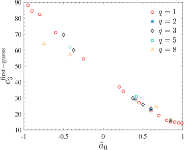
Figure 1: The first-guess $c_{3}$ values of Table 2 versus the spin variable $\tilde{a}_{0}\equiv S_{1}/(m_{1}M)+S_{2}/(m_{2}M)$. The unequal-spin and unequal-mass points can be essentially seen as a correction to the equal-mass, equal-spin values.

Figure 1 highlights that the span of the “best” (first-guess) values of $c_{3}$ is rather limited (especially for positively aligned spins) around the equal-mass, equal-spin case. At a practical level, this eases up the fitting procedure, that, following Ref. Nagar et al. (2018), is performed in two steps. First, one fits the equal-mass, equal-spin data with a quasi-linear function of $\tilde{a}_{0}=\tilde{a}_{1}+\tilde{a}_{2}$ with $\tilde{a}_{1}=\tilde{a}_{2}$. This delivers the six parameters $(p_{0},n_{1},n_{2},n_{3},n_{4},d_{1})$. Note that the analytical structure of the fitting function was chosen in order to accurately capture the nonlinear behavior of $c_{3}$ for $\tilde{a}_{0}\to 1$. In the second step one subtracts this fit, computed for the unequal-mass, unequal-spin data, from the corresponding $c_{3}^{\rm first-guess}$ values and fits the residual. This gives the parameters $(p_{1},p_{2})$. The novelty with respect to Ref. Nagar et al. (2018) is that, thanks to the new analytical improvements, one finds that the unequal-spin and unequal-mass correction can be represented, in Eq. (II.3), with acceptable accuracy, only with the two parameters $(p_{1},p_{2})$, as we shall illustrate quantitatively in Sec. IV, after an assessment of the accuracy of the NR waveforms at our disposal.

Parameter interval ranges

Waveform count $\#$

$\bar{F}_{\rm LevH/LevM}$

$q\equiv m_{1}/m_{2}$

$\chi_{1,2}$

total

with LevM

$\langle N_{\rm orb}\rangle$

$\bar{F}^{\rm max}_{\rm NR/NR}$

$\langle\bar{F}^{\rm max}_{\rm NR/NR}\rangle$

Calibration set

SXS

$[1.0,\ 10.0]$

$0$

$19$

$18$

$21.98$

$0.075\%$

$0.0092\%$

SXS

$[1.0,\ 1.0]$

$\left[-0.95,0.9942\right]$

$38$

$37$

$22.77$

$0.22\%$

$0.020\%$

SXS

$[1.3,\ 8.0]$

$\left[-0.9,0.96\right]$

$78$

$73$

$25.09$

$0.11\%$

$0.0088\%$

BAM

$[4.0,\ 18.0]$

$0$

$3$

$-$

$8.11$

$<0.1\%$

$<0.1\%$

$[2.0,\ 18.0]$

$\left[-0.85,0.85\right]$

$16$

$-$

$11.13$

$<0.1\%$

$<0.1\%$

Validation set

SXS

$[1.0,\ 10.0]$

$0$

$67$

$52$

$24.98$

$0.066\%$

$0.0050\%$

SXS

$[1.0,\ 1.16]$

$\left[-0.97,0.998\right]$

$79$

$77$

$20.29$

$0.0093\%$

$0.0029\%$

SXS

$[1.17,\ 8.0]$

$\left[-0.9,0.95\right]$

$309$

$287$

$20.74$

$0.056\%$

$0.0052\%$

long SXS

$[1.41,\ 1.83]$

$\left[-0.5,0.5\right]$

$5$

$5$

$144.05$

$1.52\%$

$0.98\%$

Table 3: Numerical Relativity datasets used in this work. From left to right, the columns report: catalog origin and use; interval of parameters covered for the mass ratio $q$ and the spins $\chi_{1,2}$; total number of waveforms in the particular sub-catalog; the number of SXS data with a second resolution LevM available; the average waveform length expressed in number of orbits, $\langle N_{\rm orb}\rangle$, counted here between the relaxation time (i.e., after the junk radiation) and the waveform amplitude peak; the absolute maximum $\bar{F}^{\rm max}_{\rm NR/NR}$ and the average of the individual maxima $\langle\bar{F}^{\rm max}_{\rm NR/NR}\rangle$ of the unfaithfulness $\bar{F}_{\rm NR/NR}$ computed between the highest, LevH, and second highest, LevM, resolutions. The $\bar{F}_{\rm NR/NR}$-uncertainties versus total mass $M$ are depicted in Fig. 2 (spinning configurations) and Fig. 20 (nonspinning configurations).

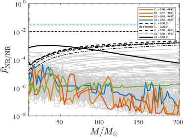
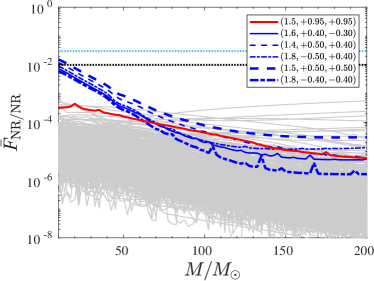
Figure 2: NR/NR unfaithfulness uncertainty computed from Eq. (48) using the highest and next to highest resolution waveform for each SXS dataset. The left panel refers to the 116 spinning waveforms used to globally inform the model (either $c_{3}$ or ringdown) that were already available the the time of Ref. Nagar et al. (2018). The right panel refers to the 393 spinning datasets recently released and discussed in Ref. Boyle et al. (2019). The same quantity for nonspinning waveforms is computed in Appendix A and shown in Fig. 20.

III Numerical Relativity waveforms

III.1 Waveforms overview

The NR data used here were separated into two categories (see Table 3). On the one hand, a set of waveforms used for the calibration of the postpeak and ringdown waveform; on the other hand, a set used for the validation of the full waveform model. The postpeak-calibration set consists of the following: (i) we enlarge the set of 23 nonspinning waveforms (19 SXS, 3 BAM, 1 test-particle) used in Nagar et al. (2019b) ; (ii) we use 38 SXS, spin-aligned, equal-mass waveforms with spins between $-0.95\leq\chi_{1,2}\leq 0.9942$, see Table 5; and (iii) 78 SXS spin-aligned, unequal-mass, waveforms going up to mass ratio $q=8$ with spins in the range $-0.9\leq\chi_{1,2}\leq 0.96$, see Tables 6 – 7, plus a single, high-quality, waveform with $(q,\chi_{1},\chi_{2})=(8,-0.9,0)$; (iv) 16 BAM, spin-aligned, unequal-mass waveforms with $2\leq q\leq 18$, encompassing two $q=8$ waveforms with $\chi_{1}=\chi_{2}=\pm 0.85$ and two $q=18$ waveforms with $\chi_{1}=\pm 0.8$ and $\chi_{2}=0$, see Table 8. All this, is complemented (v) by a sample of waveforms for a test-particle inspiralling and plunging on a Kerr black hole Harms et al. (2014) with dimensionless black hole spin $\hat{a}$ in the interval $-0.99\leq\hat{a}\leq 0.99$. The 154 NR waveforms (excluding the test-particle waveforms) in the Calibration set contain an average length of $22.35$ orbits, while the eccentricity never exceeds $0.004$.

The validation set consists of 460 waveforms from the SXS catalog SXS . The waveforms span mass ratios up to $q=8$ and spins in the range $-0.97\leq\chi_{1,2}\leq 0.998$. This set includes 5 long waveforms with an average length of $144.05$ orbits between the relaxation time and the peak of the dominant mode. The average length of the remaining waveforms is of $21.29$ orbits. Eccentricity is limited to $0.001$. The waveforms are listed in Tables 9 – 16. Further details on the SXS catalog can be found in Refs. Boyle et al. (2019); Buchman et al. (2012); Chu et al. (2009); Hemberger et al. (2013); Scheel et al. (2015); Blackman et al. (2015); Lovelace et al. (2012, 2011, 2015); Mroue et al. (2013); Kumar et al. (2015); Chu et al. (2016). The nonspinning datasets are listed in Tables 18-19.

III.2 Estimating NR uncertainties for the $\ell=m=2$ mode

The most recent update of the SXS catalog is detailed in Ref. Boyle et al. (2019). In particular, that reference gave an estimate of the NR uncertainty due to numerical truncation error on each waveform (either precessing or nonprecessing) by computing the maximal unfaithfulness (or mismatch, see below), in flat noise, between the $\ell=m=2$ waveform computed at highest and second highest resolutions available. This is found to be $\sim 10^{-4}$, that is then taken as a reliable estimate of the NR error. To ease the reader, we perform again here this uncertainty computation, although we (i) restrict it only to the case of nonprecessing waveform and (ii) we use the zero-detuned, high-power noise spectral density of Advanced LIGO aLI . The uncertainty of the BAM waveforms was estimated in Khan et al. (2016) and will be referenced and summarized for the practical purposes of this work. Considering two waveforms $(h_{1},h_{2})$, the unfaithfulness is a function of the total mass $M$ of the binary and is defined as

$$\bar{F}(M)\equiv 1-F=1-\max_{t_{0},\phi_{0}}\dfrac{\langle h_{1},h_{2}\rangle}{||h_{1}||||h_{2}||},$$ (48)

where $(t_{0},\phi_{0})$ are the initial time and phase, $||h||\equiv\sqrt{\langle h,h\rangle}$, and the inner product between two waveforms is defined as $\langle h_{1},h_{2}\rangle\equiv 4\Re\int_{f_{\rm min}^{\rm NR}(M)}^{\infty}\tilde{h}_{1}(f)\tilde{h}_{2}^{*}(f)/S_{n}(f)\,df$, where $\tilde{h}(f)$ denotes the Fourier transform of $h(t)$, $S_{n}(f)$ is the zero-detuned, high-power noise spectral density of Advanced LIGO aLI and $f_{\rm min}^{\rm NR}(M)=\hat{f}^{\rm NR}_{\rm min}/M$ is the initial frequency of the NR waveform at highest resolution, i.e. the frequency measured after the junk-radiation initial transient. Waveforms are tapered in the time-domain so as to reduce high-frequency oscillations in the corresponding Fourier transforms. Figure 2 illustrates the outcome of Eq. (48) when $(h_{1},h_{2})$ are the $\ell=m=2$ waveforms corresponding to the highest and second-highest resolution available for each SXS dataset. The left panel of Fig. 2 displays $\bar{F}(M)$ for the 116 spinning waveforms of the Calibration set; in the right panel, we have the 393 spinning waveforms in the Validation. For almost all waveforms, the uncertainty is below $0.5\%$, except for the 5 long SXS (blue in the right panel of the figure) that will deserve a dedicate discussion in Sec. III.3 below. As a very conservative, global, estimate of the NR uncertainty, we take it to be at the $0.5\%$ level. This choice is made to prevent over fitting of the NR-informed parameters, although we will see that very often a much better EOB/NR agreement arises naturally. Finally, note that the analysis of the quality of the SXS data is here limited to the uncertainties due to the numerical truncation error, because, as pointed out in Sec. 4 of Ref. Boyle et al. (2019), is the largely dominant one. The accuracy of the BAM waveforms was studied in Ref. Khan et al. (2016), considering several uncertainty sources. In particular, Figs. 2 and 3 of Ref. Khan et al. (2016) illustrate that the NR uncertainty is $\bar{F}\approx 0.1\%$ or less. Similarly to the SXS case, and to avoid overfitting and be conservative, we assume the uncertainties on alla BAM waveforms at the $0.3\%-0.5\%$ level and use this as target for EOB/NR comparisons.

III.3 Long-inspiral Numerical Relativity waveforms

Let us comment on the 5, very-long, waveforms listed in Table 17. All these waveforms show an inspiral of over 100 orbits before a common horizon appears. The unfaithfulness between the two highest resolution levels is shown as blue lines in Fig. 2. All dataset show a rather large $\bar{F}$ for low masses, up to $1.5\%$ for SXS:BBH:1415, that then decreases to the average $\bar{F}$ around $60M_{\odot}$. This suggests that the long inspiral is more sensitive to resolution and/or other systematics effects, so that the numbers of Fig. 2 should be taken as a rather conservative uncertainty estimates.

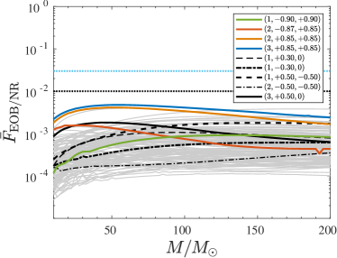
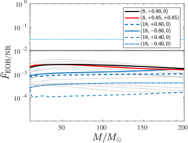
Figure 3: EOB/NR unfaithfulness for the $\ell=m=2$ mode obtained from Eq. (48). Left panel: computation using SXS waveforms publicly released before February 3, 2019. Right panel: same computation done with BAM waveform data. As explained in Sec. II.3, a subset of all this data (see Table 2) is used to inform the $c_{3}$ EOB function. Comparison with Figs. 1 and 3 of Ref. Nagar et al. (2018) allows one to appreciate the improvement with respect to the original implementation of TEOBResumS. Comparison with Fig. 2 highlights that the $\bar{F}_{\rm EOB/NR}$ is either of the order of, or larger than the NR/NR uncertainties.

IV The $\ell=m=2$ mode: EOB/NR unfaithfulness

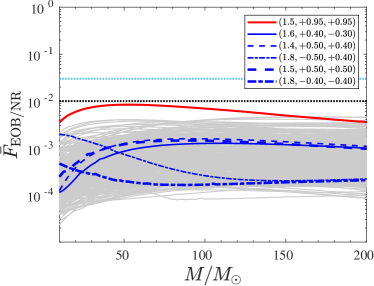
Figure 4: EOB/NR $\ell=m=2$ unfaithfulness computation with SXS waveform data publicly released after February 3, 2019. None of these datasets was used to inform the model in the dynamical EOB functions $(a_{6}^{c},c_{3})$, although several were used for the postmerger waveform part. It is remarkable that $\bar{F}^{\rm max}_{\rm EOB/NR}$ is always below $0.4\%$ except for a single outlier, red online, that however never exceeds $0.85\%$. The plot includes five exceptionally long waveforms, each one developing more than 139 GW cycles before merger, SXS:BBH:1412, 1413, 1414, 1415 and 1416 (blue online).

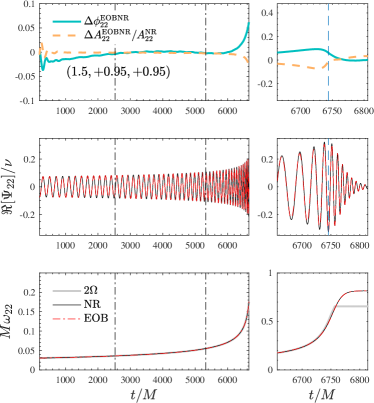
Figure 5: Improved EOB/NR phasing comparison for SXS:BBH:1146 when the value of $c_{3}^{\rm fit}=15.96$ used in Fig. 4 is lowered to $c_{3}=11.1$. Top panel: (relative) amplitude and phase differences. Middle panel: real part of the waveform. Bottom panel: gravitational frequencies. For convenience, also twice the EOB orbital frequency $2\Omega$ is shown on the plot. The dash-dotted vertical lines indicate the alignment frequency region, while the dashed one the merger time. This comparison illustrates that SXS:BBH:1146 is an outlier in Fig. 4 only because of the rather limited amount of NR waveforms used to inform $c_{3}^{\rm fit}$.

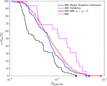
Figure 6: Global representation of $\bar{F}_{\rm EOB/NR}^{\rm max}$ all over the SXS (595) and BAM (19) NR simulations. The various SXS subsets, nonspinning (black online, 89 waveforms), merger-ringdown calibration (blue online, 116 spin-aligned waveforms) and validation (red online, 388 spin-aligned waveform) discussed in the text are represented separately. The plot shows the fraction (expressed in $\%$) $n/N_{\rm set}$, where $N_{\rm set}$ is the total number of waveforms in a given NR-waveform set and $n$ is the number of waveforms, in the same set, that, given a value $\bar{F}$, have $\bar{F}^{\rm max}_{\rm EOB/NR}\geq\bar{F}$. The colored marker highlight the largest values in each NR dataset. Note that this plot incorporates 460 new SXS waveforms that were not included in Fig. 6 of Nagar et al. (2018).

We start now discussing the performance of the analytical waveform model in terms of EOB/NR unfaithfulnesses plots for the $\ell=m=2$ mode, obtained computing Eq. (48) between EOB and NR waveforms. Both EOB and NR waveforms are tapered in the time-domain so as to reduce high-frequency oscillations in the corresponding Fourier transforms. Figure 4 illustrates $\bar{F}$ versus $M$ evaluated over the same NR waveform data used in Ref. Nagar et al. (2018), with the SXS data in the left panel and the BAM data in the right panel. As mentioned above, a subset of this data, listed in Table 2, (both SXS and BAM) was used to inform the $c_{3}(\nu,\tilde{a}_{1},\tilde{a}_{2})$ function. The global performance of the model is largely improved with respect to Ref. Nagar et al. (2018), see Fig. 1 there. Remarkably, the model performs excellently also for large mass ratios and large spins, without any outlier above the $1\%$ threshold, but $\bar{F}^{\rm max}_{\rm EOB/NR}\lesssim 0.5\%$ all over.

After February 3, the SXS collaboration publicly released another 455 new simulations at an improved accuracy. This part of the catalog mostly covers the same region of parameter space of the previous data, except for a few waveforms spanning mass ratios between 4 and 8, with spins higher than what considered before. The catalog also includes a few extremely long waveforms, with more than 100 orbits. As an additional cross check of the robustness and accuracy of our model, we compute $\bar{F}_{\rm EOB/NR}$ all over this new set of NR waveforms. The result is displayed in Fig. 4. We find that $\bar{F}^{\rm max}_{\rm EOB/NR}$ always remains below $0.85\%$, a value reached only by one dataset, $(1.5,+0.95,+0.95)$ SXS:BBH:1146, while for all others we have $\bar{F}^{\rm max}_{\rm EOB/NR}\lesssim 0.4\%$. This is not surprising since the set of NR waveforms used to inform $c_{3}$ does not cover, except for one single dataset with $(1.5,-0.5,0)$, the parameter space with $1<q<2$. In this respect, to better understand the behavior of this outlier in Fig. 4 we checked that $c_{3}^{\rm fit}(1.5,+0.95,+0.95)=15.96$ yields an accumulated EOB/NR phase difference $\sim 4.7$ rad at merger once the two waveforms are aligned during the inspiral. Interestingly, by lowering the value of $c_{3}$, and thus increasing the magnitude of the spin-orbit effective coupling and thus making the EOB waveform longer, we can easily reconcile it with the NR data. For convenience we illustrate this result in Fig. 5, that is obtained with $c_{3}=11.1$ (the two dash-dotted vertical lines indicate the alignment region). We also point the reader to Table 11, where the NR uncertainty for this dataset is estimated to be $\bar{F}_{\rm NR/NR}=0.0446\%$. On a different note, this suggests that the current model could be additionally, and easily, improved by also considering SXS:BBH:1146 to inform $c_{3}^{\rm fit}$. Yet, this results highlights the robustness of our model: without any additional input from NR simulations to determine $c_{3}$, it is able to deliver rather accurate waveforms even in a region of the parameter space previously not covered by NR data. The model performance is summarized in Fig. 6. For each dataset considered above, the figure exhibits the fraction of waveform whose $\bar{F}_{\rm EOB/NR}^{\rm max}$ is larger or equal a given value $\bar{F}$. Thanks to the additional analytical information incorporated and to the improved waveform resummation, TEOBiResumS_SM is currently the EOB model that exhibits the lowest EOB/NR unfaithfulness for the $\ell=m=2$ mode.

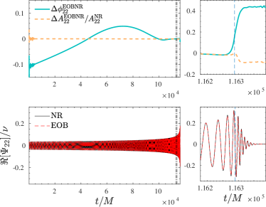
Figure 7: EOB/NR phasing comparison for SXS:BBH:1415, $(1.5,+0.50,+0.50)$. Note that it doesn’t seem possible to flatten the phase difference up to $t/M\simeq 1\times 10^{5}$. The vertical lines indicate the alignment frequency region $[M\omega_{L},M\omega_{R}]=[0.038,0.042]$. See text for additional discussion.

IV.1 Long-inspiral Numerical Relativity waveforms

It is interesting to note that the 5, long, NR simulation exhibit an excellent agreement ($\bar{F}_{\rm EOB/NR}\simeq 10^{-3}$, see Fig. 4) with the analytical waveform , even during the long inspiral phase. Note that this is below the NR-uncertainty estimate in the right panel of Fig. 2 without any input in the model coming from this data. Despite such good agreement for the usual standard, an illustrative time-domain comparison done for SXS:BBH:1415, see Fig. 7, highlights some features that is worth commenting on. At first glance, the phase agreement is excellent for any standard quality assessment, always between $\pm 0.1$ rad. However, contrary to our expectations, we didn’t succeed in flattening the phase difference by aligning the EOB and NR waveform during the early inspiral. This is usually achieved by narrowing the alignment frequency window $[M\omega_{L},M\omega_{R}]$ and moving it to early-inspiral frequency values. By contrast, to achieve a rather flat phase difference on a reasonably large time-interval we had to progressively displace interval the frequency window to higher frequencies, until hitting $[M\omega_{L},M\omega_{R}]=[0.038,0.042]$, that corresponds to the two, dash-dotted, vertical lines in Fig. 7. In view of the rather large uncertainty on this NR waveform, we cannot really state whether this is due to some systematics in the NR waveforms or in missing physics within the EOB model. Additional analyses done using more sophisticated phasing diagnostics, e.g. the gauge-invariant $Q_{\omega}\equiv\omega^{2}/\dot{\omega}$ function Baiotti et al. (2010, 2011); Damour et al. (2013), where $\omega\equiv\dot{\phi}$ is the gravitational wave frequency, might be necessary to better investigate the low-frequency consistency between the EOB and NR waveforms. An analogous behavior is shared also by the other long-term waveforms. However Fig. 4 highlights that the $\bar{F}_{\rm EOB/NR}$ for SXS:BBH:1414 $(1.83,-0.5,+0.4)$ and SXS:BBH:1416 $(1.78,-0.4,-0.4)$ show a qualitatively different behavior, with $\bar{F}_{\rm EOB/NR}$ that is starting at a slightly increased value for $M=10M_{\odot}$ and then is progressively decreasing with $M$. When aligning the waveforms in the same frequency interval $[0.038,0.042]$, so to obtain a quasi-flat phase difference also outside the alignment window, one finds that the EOB/NR phase difference grows linearly backwards for $10^{5}M$, to reach the $0.5$-$0.7$ rad at the beginning of the inspiral. Although this fact might explain the behavior of $\bar{F}_{\rm EOB/NR}$ seen in Fig. 4, conclusive NR-quality assessments require more detailed investigations that are postponed to future work.

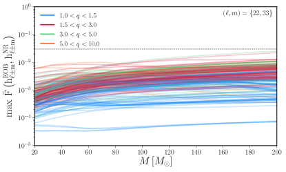
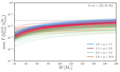
Figure 8: EOB/NR unfaithfulness computation putting together all $\ell=m$ modes up to $\ell=4$. Plotted is the worst-case performance maximing the unfaithfulness over the sky, Eq.(49). The worst-case mismatches arise from near edge-on configurations, when the power emitted in the $(2,2)$ mode is minimized.

V Higher multipolar modes

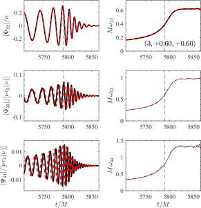
(a)     (b)

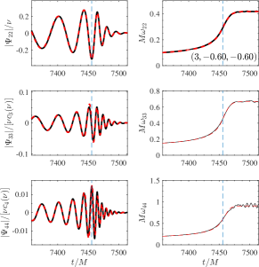
(c)     (d)

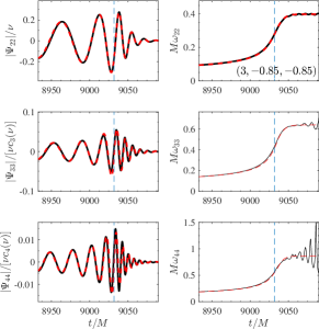
Figure 9: Behavior of $(2,2)$, $(3,3)$ and $(4,4)$ modes for a few, illustrative, spin-aligned configurations with $q=3$: comparing NR (black) with EOB (red) waveform. Each panel plots the real part (left columns) and the instantaneous frequency (right columns).

V.1 Multipoles $(2,2)$, $(3,3)$ and $(4,4)$

Let us move now to discussing the quality of the higher modes. For illustrative purposes, we consider explicitly four configurations with $q=3$, with equal spins, both aligned or anti-aligned to the orbital angular momentum. More precisely, we use $(3,-0.85,-0.85)$, $(3,-0.60,-0.60)$, $(3.-0.30,-0.30)$ and $(3,+0.60,+0.60)$. The qualitative (and quantitative) behavior discussed here for this configuration is general enough to be considered paradigmatic all over the SXS waveform catalog. Figure 9 illustrates the behavior of the $(2,2)$, $(3,3)$ and $(4,4)$ mode. For each multipoles, we show the real part of the EOB/NR waveforms together with the instantaneous GW frequency $\omega_{{\ell m}}$. The EOB waveform is aligned to the NR one around merger, so to highlight the excellent EOB/NR agreement there. The EOB/NR agreement is rather good either for spins both anti-aligned or aligned with the orbital angular momentum. We should, however, mention that when the spins are large and aligned there is an increasing dephasing accumulating between the EOB and NR $(4,4)$ mode, as one can see in Fig. 9 (a). As it was the case for the $\ell=m=2$ mode discussed above, a global understanding of the actual performance of the model comes from EOB/NR unfaithfulness computations. In addition to Eq. (48), due to the non-trivial angular dependence introduced by the subdominant spherical harmonics, we consider the worst-case performance of the model by maximizing the unfaithfulness over the sky

$$\max\;\bar{F}(h_{1},h_{2})\equiv\max_{\theta,\phi}\;\bar{F}(h_{1},h_{2}).$$ (49)

In Fig. 8, we show the worst case performance for the $\ell=m$ modes up to $\ell=4$, finding excellent agreement up to $\sim 120M_{\odot}$ above which the model performance degrades slightly and moves above 3%. In all cases, the worst case mismatches arise from near edge-on configurations, where the power in the (2,2)-mode is minimized. The worst mismatches occur for mass ratios $1\leq q\leq 1.5$ and equal-spin configurations, in which the approximate symmetry of the binary leads to a suppression of odd-$m$ modes. For these binaries, the degraded performance will be driven by the accuracy of the $(4,4)$ mode in both the EOB model and the underlying NR data itself.

V.2 Other subdominant multipoles

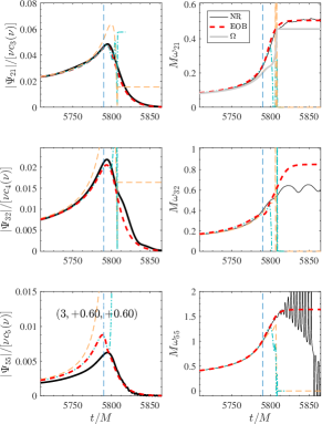
(a)     (b)

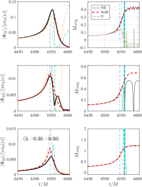
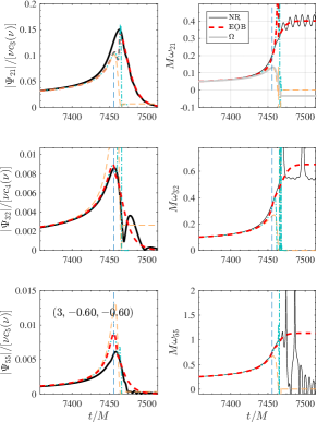
(c)     (d)

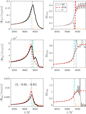
Figure 10: Frequency and amplitude for the $(2,1)$, $(3,2)$ and $(5,5)$ modes for the same BBH configurations of Fig. 9. On top of the NR (black) and complete EOB curves (red, dashed), the plots also show: (i) the analytical EOB waveform, without NQC corrections and ringdown (orange online) and (ii) the NQC-augmented EOB waveform (light-blue online). The dashed, vertical, line marks the merger location, i.e. the peak of the $\ell=m=2$ waveform amplitude. The $(2,1)$ frequency plots also incorporate the orbital frequency $\Omega$ (grey online). The construction of the $(2,1)$ mode through merger and ringdown cannot be accomplished correctly for large values of the spins anti-aligned with the orbital angular momentum [see panel (c) and (d)].

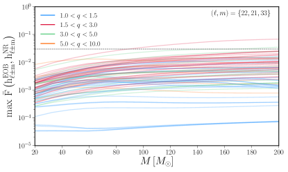
Figure 11: EOB/NR unfaithfulness, maximized over the direction from the sky, when including $(2,2)$, $(2,1)$ and $(3,3)$ modes. Here we only consider a subset of the SXS waveforms with $\chi_{i}>-0.4$, where the $(2,1)$ EOB waveform mode does not present pathologies (see Fig. 10). The worst case configuration is SXS:BBH:0239, a binary of mass ratio and spins $(2.0,-0.37,+0.85)$.

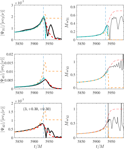
Figure 12: Illustrative EOB/NR comparison for modes $(3,1)$, $(4,3)$ and $(4,2)$ for $(3,+0.3,+0.3)$. This behavior is analogous to the nonspinning case and is robust until the spins are mild. For larger spins, these modes may suffer the same problem related to the NQC factor discussed above for the $(2,1)$ mode.

V.2.1 Multipoles $(2,1)$, $(3,2)$ and $(5,5)$

Let us discuss now modes $(2,1)$, $(3,2)$ and $(5,5)$, that can be robustly constructed over most (but crucially not all) the parameter space. To illustrate the typical behavior, we consider the same BBH configurations show in Fig. 9, but we focus now on amplitude and frequency. Each panel of the figure compares four curves: the NR one (black), the analytical EOB waveform (orange), the NQC-corrected EOB waveform (light-blue) and the complete EOB waveform that includes the ringdown part. In addition, on the $(2,1)$ frequency we also superpose the EOB orbital frequency, as a grey line. The blue, dashed, vertical lines in the plot mark the location of the merger point, i.e. the peak of the $(2,2)$ waveform amplitude. A few considerations first on the NR waveforms: during the ringdown, one clearly sees in the $(2,1)$ and $(3,2)$ the effect of mode mixing, that shows up as amplitude modulations and frequency oscillations. The origin of these features has been explained in details in Ref. Taracchini et al. (2014). By contrast, the $(5,5)$ mode shows features that clearly highlight some lack of accuracy in the NR data. This is more evident in both $(3,-0.60,-0.60)$ and $(3,-0.85,-0.85)$ configurations (see bottom rows of the (c) and (d) panels of Fig. 10. Let us focus first on the $(3,2)$ mode. Despite the absence of mode-mixing, the complete EOB waveform qualitatively reproduces the behavior of the NR one around peak and postpeak, especially for what concerns the amplitude. By contrast, the ringdown frequency, i.e. in the postpeak regime, is flat and systematically larger than the NR one because of lack of the physical information in the ringdown modelization. It is however interesting to note that the approximation is more reliable for large, anti-aligned, spins. Similarly, the shape of the waveform entailed by the action of the NQC is rather accurate and yields a reliable approximation of the frequency behavior up to merger. By contrast, the situation is different for the $(2,1)$ mode. When spins are aligned with the angular momentum, the standard procedure for improving the behavior of the merger waveform via NQC and the ringdown attachment works well, consistently with the nonspinning case discussed in Ref. Nagar et al. (2019b). This is clear for the case $(3,+0.60,+0.60)$ of Fig. 10 and the procedure remains robust at least up to $(3,-0.30,-0.30)$ as the figure illustrates. By contrast, as the magnitude of the anti-aligned spins increase, the NQC correction becomes progressively inaccurate and the resulting waveform becomes incompatible with the NR ones. This is for example the case for $(3,-0.85,-0.85)$, where the NQC correction is unable to act so as to smoothly connect the inspiral, plunge and merger waveform to the ringdown (postmerger) part. This latter is, by contrast, reliable, except for the mode-mixing oscillation, that is missing by construction. We tracked the reason of the unphysical behavior of the NQC correction as follows. In our approach, that is the same of the nonspinning case, Paper I, the NR information used to determine the NQC parameters is extracted $2M$ after the $(2,1)$ peak. As a consequence, for a successful implementation, the NQC factor should be evaluated there. Unfortunately, the EOB dynamics in this region, that is after merger time (i.e. the peak of the $(2,2)$ mode), may develop unphysical features depending on the values of the spins. The simplest way to explain what is going on is by looking at the orbital frequency, $\Omega$. This is shown as a grey line in the $(2,1)$ panels of Fig. 10. One sees that for both $(3,-0.60,-0.60)$ and $(3,-0.85,-0.85)$ $\Omega$ becomes very small around the peak of the $(2,1)$ mode until it crosses zero and becomes negative. This is unexpected for this configuration and not what it is supposed to be. The unphysical character of this feature can be understood by qualitative comparison with the system made by a point-particle inspiralling and plunging on a Kerr black hole. In this case, the orbital frequency changes sign for configurations where the spin of the black hole is antialigned with the orbital angular momentum and large: the frame dragging exerted by the black-hole space time on the particle is responsible of the sign change in the frequency (see e.g. Ref. Harms et al. (2014) ). One should be aware that such dynamical behavior reflects on the waveform, and in particular on the QNMs frequency excitations, notably also at the level of the $(2,2)$ mode, that should have a zero at the time when the angular velocity of the particle changes sign (i.e., from counterrotation with respect to the black hole, to rotating with the black hole). Such qualitative features are not present in the NR waveform, so we believe that the EOB frequency behavior for this configuration is incorrect after merger time. This suggests that the current Hamiltonian should be modified so to avoid this feature. At a practical level, the fact that $\Omega$ crosses zero when the values of the relative separation $r$ is small, but finite, implies that the NQC functions $n_{4}\equiv p_{r_{*}}/(r\Omega)$ and $n_{5}\equiv p_{r_{*}}/(r\Omega)\Omega^{2/3}$ (see Paper I) become very large and prevent the related NQC correction to the phase to act efficiently so to correctly modify the bare inspiral waveform. This is is evident in panel (c) and (d) of Fig. 10. This problem affects the $(2,1)$ for any mass ratio when the anti-aligned spin(s) are sufficiently large. For example, a similar behavior is found also for $(8,-0.90,0)$. As a consequence, to use the current multipolar model for actual parameter estimation studies, it will be necessary to determine the precise region of the parameter space where the $(2,1)$ mode is reliable. Selecting only those datasets with $\chi_{i}>-0.4$, Fig. 11 shows the EOB/NR unfaithfulness, maximized over the sky, when including modes $(2,2)$, $(2,1)$ and $(3,3$. Further improvement, as well as the determination of the precise range of reliability of the $(2,1)$ mode through merger and ringdown, are postponed to future work. Here we will just briefly explore, in Sec. V.2.3 below, a possible modification to the current spin-orbit sector of the Hamiltonian that may eventually improve the behavior of the $(2,1)$ mode in the anti-aligned spin case.

V.2.2 Multipoles $(3,1)$, $(4,3)$ and $(4,2)$

From fits of the SXS waveforms we can also obtain a postmerger/ringdown description of the $(3,1)$, $(4,2)$ and $(4,3)$ modes. For simplicity and robustness, the $(3,1)$ ringdown relies on the nonspinning fits of Ref. Nagar et al. (2019b), while for $(4,3)$ and $(4,2)$ the relevant information is found in Appendix C.2.7-C.2.6. When the magnitude of the spins are relatively mild, these modes can be modeled rather accurately (modulo mode mixing during ringdown) as in the nonspinning case Nagar et al. (2019b). Figure 12 illustrates this fact for $(3,+0.30,+0.30)$, with the usual EOB/NR comparison as we did above. For $(4,3)$ and $(4,2)$ modes one can appreciate the relevant action of the NQC factor. When spins are larger (and notably anti-aligned) one can have $\Omega$-driven pathological effects like the $(2,1)$ mode discussed above. Seen also the (average) lower accuracy of the corresponding NR modes all over the SXS catalog, we postpone a more detailed discussion (and possible improvements) to future work.

V.2.3 Improving the behavior of the $(2,1)$ multipole

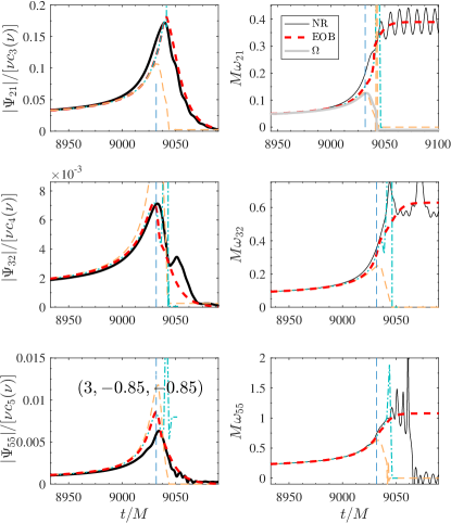
Figure 13: Attempt of improving the behavior of the $(2,1)$ mode for $(3,-0.85,-0.85)$ by modifying the spin-orbit sector of the EOB Hamiltonian. The related change in the EOB orbital frequency, $\Omega$, that is seen now to decrease more mildly after its peak than in Fig. 10 (d), is sufficient to improve the efficiency of the NQC correction, so to get a more acceptable frequency growth that can be smoothly connected with the ringdown. See text for additional details.

The correct behavior of the orbital frequency $\Omega$ in the strong-field regime is determined by subtle compensation between the orbital and spin-orbit part of the Hamiltonian. This is the region where our analytical understanding is weaker, as we have to rely on resummed results that are analytically incomplete. From the practical point of view, to NQC-complete the inspiral $(2,1)$ mode following the current scheme it would be sufficient the behavior of $\Omega$ be milder after the merger. In practice, we found that this is possible by implementing a small modification to the resummed $(G_{S},G_{S_{*}})$ functions. The spin-orbit sector of the Hamiltonian is based on Ref. Damour and Nagar (2014a), in particular the gyro-gravitomagnetic functions are given by Eqs. (38), (39), (41), and (42), where the inverse separation $u$ is replaced by the inverse centrifugal radius $u_{c}$. While $G_{S}^{0}=2uu_{c}^{2}$, Eq. (38) of Ref. Damour and Nagar (2014a), has the structure of the Kerr gyro-gravitomagnetic function, the dependence of $u_{c}$ introduced in the other functions, $G_{S_{*}}^{0}$, $\hat{G}_{S}$ and $\hat{G}_{S_{*}}$ was an arbitrary choice. One finds that replacing such $u_{c}$ dependence with the, more natural, $u$-dependence is sufficient to provide small modifications in the behavior of $\Omega$ that entail a far more robust behavior of the NQC correction. In practice, we use

$$G_{S} =2uu_{c}^{2}\hat{G}_{S}(u),$$ (50)

$$G_{S_{*}} =\dfrac{3}{2}u^{3}\hat{G}_{S_{*}}(u),$$ (51)

where $(\hat{G}_{S},\hat{G}_{S_{*}})$ are given by Eqs. (41)-(42) of Ref. Damour and Nagar (2014a) where $u_{c}$ is replaced by $u$. The result of this change for $(3,-0.85,-0.85)$ is illustrated in Fig. 13. Note that, since the dynamics has now changed, to get a good $(2,2)$ EOB/NR phasing agreement we had to use $c_{3}=86.5$ instead of $c_{3}^{\rm fit}=79.98$ from Eq. (II.3). Comparing Fig. 13 with the panel (d) of Fig. 10 one immediately notices the different behavior of the orbital frequency, whose peak is shallower than before. The consequence of this behavior is that the action of the NQC factor on both amplitude and frequency is more correct than before, though not yet fully accurate for this latter. Although improvable, this proves that the scheme for completing the EOB waveform through merger and ringdown for all modes that was seen to be efficient in the nonspinning case Nagar et al. (2019b) can be straightforwardly generalized to the spinning case provided the dynamics, i.e. the orbital frequency, behaves correctly. The result of Fig. 13 gives us a handle to improve the description of spin-orbit effects within the EOB Hamiltonian in future work.

Table 4: Frequency of the minimum of the $(2,1)$ amplitude for a few BBH configurations considered in Ref. Cotesta et al. (2018) and not publicly available. $M\Omega_{0}$ is the (orbital) frequency corresponding to a minimum (or a zero) in the amplitude. Our EOB-predicted value, from the zero of $\hat{f}_{21}^{\rm S}$ in Table 1, is more consistent with the NR one than the straightforward PN value.

Name	$q$	$\chi_{1}$	$\chi_{2}$	$\hat{S}$	$\!\!M\Omega_{0}^{\rm NR}$	$\!\!\!M\Omega_{0}^{\rm EOB}$	$M\Omega_{0}^{\rm PN}$
SXS:BBH:0614	2	0.75	$-0.5$	0.278	0.083	0.0968	0.057
SXS:BBH:0612	1.6	0.5	$-0.5$	0.115	0.068	0.0712	0.047
SXS:BBH:1377	1.1	$-0.4$	$-0.7$	$-0.268$	0.033	0.0330	0.029

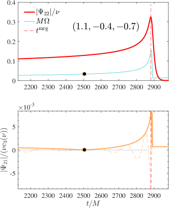
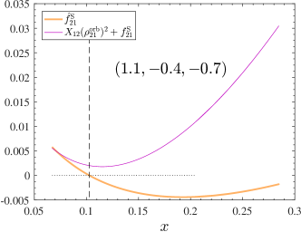
Figure 14: Top and medium panels: occurrence of a zero in the $(2,1)$ amplitude in configuration $(1.1,-0.4,-0.7)$, corresponding to NR dataset SXS:BBH:1377 analyzed in Ref. Cotesta et al. (2018). This dataset is not publicly available through the SXS catalog. The EOB-predicted value of the frequency is perfectly compatible with the NR value reported in Ref. Cotesta et al. (2018) (see the last row of Table 4). The bottom panel compares the zero location of the resummed (orange) and nonresummed (magenta) amplitudes. See text for details.

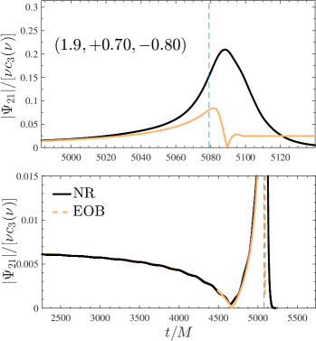
Figure 15: Mode $(2,1)$: comparison between the EOB amplitude (orange) and the corresponding NR one from dataset SXS:BBH:1466. The purely analytical EOB waveform multipole can accurately predict the location of the minimum (that analytically is a zero of the modulus) consistently with the one found in the NR data. The excellent agreement shown is obtained naturally, without the need of calibrating any additional parameter entering the waveform amplitude. The dashed vertical line corresponds to merger time, i.e. the peak of the $\ell=m=2$ waveform. The cusp in the analytical amplitude occurs because of a zero in $\hat{f}_{21}^{\rm S}$ as illustrated in Fig. 16.

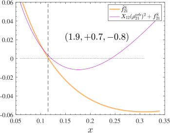
Figure 16: Complementing Fig. 15: the behavior of the resummed versus nonresummed amplitude versus $x=\Omega^{2/3}$.

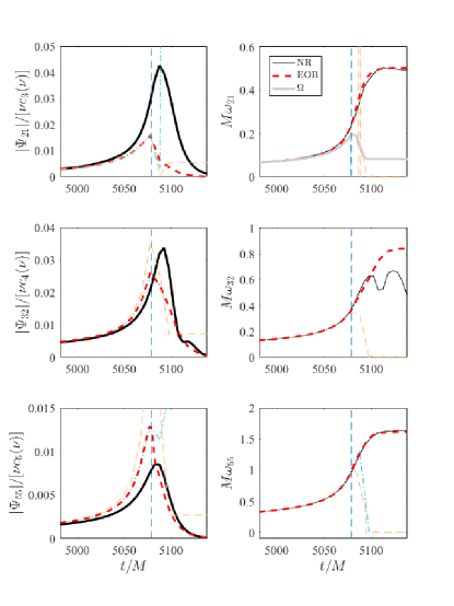
Figure 17: EOB/NR waveform comparison for SXS:BBH:1466 for modes $(2,1)$, $(3,2)$ and $(5,5)$. The frequency of the $(2,1)$ mode behaves correctly through merger and ringdown, while the EOB amplitude largely underestimates the NR one. As in Fig. 10, the orange curve is the purely analytical EOB waveform, while the light blue one is the NQC corrected. The vertical line marks the merger location

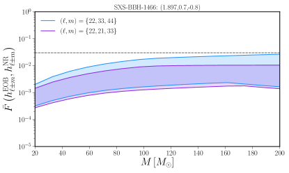
Figure 18: The minimum and maximum EOB/NR unfaithfulness for SXS:BBH:1466 over the whole sky. The blue curve uses the $(2,2),(3,3)$ and $(4,4)$ modes. The purple curve uses the $(2,2),(2,1)$ and $(3,3)$ modes. Worst case mismatches occur near edge on configurations with the unfaithfulness being below 3% up to $200M_{\odot}$.

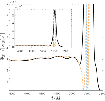
Figure 19: Mode $(3,1)$: comparison between the EOB amplitude (orange) and the corresponding NR one from dataset SXS:BBH:1496, $(1.1584,+0.7997,+0.0285)$. While the analytical waveform has a zero because of $\hat{f}_{31}$, the NR one just shows a glimpse of a global minimum, probably because if insufficient numerical resolution. Note however the excellent qualitative and quantitative consistency between the two waveforms up to that point.

V.3 Peculiar behavior of $\bm{m=1}$ waveform amplitudes for $\bm{1\leq q\leq 2}$.

Reference Cotesta et al. (2018) pointed out that a few NR simulations exhibit a minimum in the $(2,1)$ mode amplitude in the late inspiral phase. Such behavior was found in 4 SXS datasets: SXS:BBH:0254 $(2,+0.6,-0.6)$; SXS:BBH:0612 $(1.6,0.5,-0.5)$; SXS:BBH:0614 $(2,+0.75,-0.5)$; and SXS:BBH:1377 $(1.1,-0.4,-0.7)$. Only the first among these dataset if public through the SXS catalog. In addition, Ref. Cotesta et al. (2018) noticed that the same feature is present in the EOB resummed waveform (both in orbital-factorized and non-orbital factorized form). An explanation of this phenomenon was suggested on the basis of leading-order considerations, that were similarly proven using a 3PN-based analysis. In addition, Ref. Cotesta et al. (2018) compared the PN prediction for the frequency corresponding to the minimum of the $(2,1)$ mode with the value extracted from NR simulations. From this PN-based analysis, Ref. Cotesta et al. (2018) suggested that the phenomenon comes from a compensation between the spinning and leading-order nonspinning terms entering the $(2,1)$ mode. Notably, the PN based analysis aimed at explaining this feature qualitatively as well as semi-quantitatively (see Table I in Ref. Cotesta et al. (2018)).

Here we revisit the analysis of Ref. Cotesta et al. (2018) and we attempt to improve it along several directions thanks to the robustness of our factorized and resummed waveform amplitudes. In brief we can show that: (i) focusing on the same datasets considered in Ref. Cotesta et al. (2018), we illustrate that the $(2,1)$, purely analytical EOB amplitude has a minimum (in fact, a zero) rather close to the values reported in Table I of Ref. Cotesta et al. (2018), and definitely much closer than the PN-based prediction; (ii) the phenomenon is here understood as coming from the compensation, occurring at a given frequency, between the two (inverse-resummed) macro-terms that compose the analytically resummed expression of $\hat{f}_{21}^{S}$, one proportional to $X_{12}$ and the other one proportional to $\tilde{a}_{12}$, and that appear with opposite signs; (iii) guided by this analytical understanding, we investigated whether some of the currently available simulations in the SXS catalog may develop a zero (that occurs in fact as a cusp) in the amplitude. Quite remarkably we found that it is indeed the case for SXS:BBH:1466, $(1.9,+0.70,-0.8)$, that shows a clean minimum that is perfectly consistent with the EOB-based analytical prediction; (iv) since the same structure, with the minus sign, is present also in other $m=\text{odd}$ modes, we investigated whether the same phenomenon may show up also in some of the other SXS datasets. Interestingly, we found that also the $(3,1)$ mode of SXS:BBH:1496 is consistent with the EOB-predicted analytical behavior, suggesting that such features may occur in several modes.

Let us now discuss in detail the four points listed above. Figure 14 illustrates an EOB analytical waveform for $(1.1,-0.4,+0.7)$, that corresponds to the dataset SXS:BBH:1377. As mentioned above, this simulation is not public and so we cannot perform an explicit EOB/NR comparison. The top panel shows the $\ell=m=2$ waveform amplitude together with the EOB orbital frequency $M\Omega$. The middle panel shows the $(2,1)$ waveform amplitude, that develops a zero highlighted by a marker. It turns out that this zero precisely corresponds to the zero of the $\hat{f}_{21}^{\rm S}$ function once evaluated at $x=(M\Omega)^{2/3}$. This function is shown, versus $x$, in the bottom panel of Fig. 14. To be more quantitative, the last row of Table 4 lists the corresponding frequency, that is identical to the NR-extracted value reported in the corresponding last column of Table I of Cotesta et al. (2018). To check the model further, we explored also the other two cases in the Table, similarly finding a rather good agreement between the EOB orbital frequency corresponding to the zero and the NR value. Our reasoning relies on our orbital factorized waveform, and in particular on the definition of $\hat{f}_{21}^{\rm S}$. However, Ref. Cotesta et al. (2018) pointed out that a zero in the amplitude may occur also in the standard, non orbital-factorized, waveform amplitude. To make some quantitative statement, we also consider the function

$$f_{21}^{\rm orb+S}=X_{12}\left(\rho^{\rm orb}_{21}\right)^{2}+f_{21}^{\rm S},$$ (52)

where both $\rho_{21}^{\rm orb}$ and $f_{21}^{\rm S}$ are kept in PN-expanded form. The orbital term is given in the usual Taylor-expanded form $\rho_{21}^{\rm orb}=1+(\dots)x+(\dots)x^{2}+(\dots)x^{3}+(\dots)x^{4}+(dots)x^{5}$. The spin term, at NNLO, reads

$$f_{21}^{\rm S}=-\dfrac{3}{2}\tilde{a}_{12}x^{1/2}+c_{\rm SO}^{\rm NLO}x^{3/2}+c_{\rm SS}^{\rm LO}x^{2}+c_{\rm SO}^{\rm NNLO}x^{5/2},$$ (53)

where

$$c_{\rm SO}^{\rm NLO} =\left(\dfrac{110}{21}+\dfrac{79}{84}\nu\right)\tilde{a}_{12}-\dfrac{13}{84}\tilde{a}_{0}X_{12},$$ (54)

$$c_{\rm SS}^{\rm LO} =-\dfrac{27}{8}\tilde{a}_{0}\tilde{a}_{12}+\dfrac{3}{8}X_{12}\left(\tilde{a}_{1}^{2}+\dfrac{10}{3}\tilde{a}_{1}\tilde{a}_{2}+\tilde{a}_{2}^{2}\right),$$ (55)

$$c_{\rm SO}^{\rm NNLO} =\left(-\dfrac{3331}{1008}-\dfrac{13}{504}\nu+\dfrac{613}{1008}\nu^{2}\right)\tilde{a}_{12}$$

$$+\left(-\dfrac{443}{252}+\dfrac{1735}{1008}\right)\tilde{a}_{0}X_{12}+\dfrac{3}{4}\tilde{a}_{0}^{2}\tilde{a}_{12}.$$ (56)

For the configuration $(1.1,-0.4,-0.7)$, this function, represented versus $x$, does not have a zero, as illustrated by the magenta line in the bottom panel of Fig. 14.

The closeness between the numbers in Table 4 prompted us to additionally investigate for which values of spin and mass ratio the analytical $(2,1)$ amplitude develops a zero before merger frequency. Comparing with the configurations available through the SXS catalog (notably those up to February 3, 2019), we found that the parameters of dataset SXS:BBH:1466 are such that the zero in the amplitude occurs at a frequency that is smaller than the merger frequency. We then explicitly checked the $(2,1)$ mode of this simulation and, as illustrated in Fig. 15, we found that it has a local minimum, that is very consistent with the cusp in the analytic EOB waveform modulus. In addition, Fig. 17 illustrates the behavior of the full waveform completed by NQC corrections and ringdown. As above, we show together the more difficult modes to model, $(2,1)$ and $(3,2)$, with $(5,5)$. The figure highlights that the $(2,1)$ frequency is well captured by the analytical model, although the amplitude is underestimated by more than a factor two. Consistently, Fig. 18 shows that the minimum and maximum unfaithfulness over the whole sky is always below $3\%$. This makes us confident that TEOBiResumS_SM can give a reliable representation of the $(2,1)$ mode also in this special region of the parameter space, since it naturally incorporates a feature that is absent in SEOBNRv4HM Cotesta et al. (2018). One should however be aware that the $(2,1)$ EOB mode is not as good for the case $(2,+0.60,-0.60)$, where the corresponding NR waveform is found to have very a clean minimum much closer to the merger frequency, as noted in Ref. Cotesta et al. (2018). This is probably due to lack of additional analytical information to improve the behavior of the $(2,1)$ mode in the strong-field regime. It would be interesting to investigate, for future work, whether higher-order PN terms (e.g. those obtained after hybridization with test-mass results, similarly to the procedure followed for the $m=$ even) could be useful to improve the behavior of the $(2,1)$ EOB amplitude for $(2,+0.60,-0.60)$.

As a last exploratory study, we investigated whether some of the other $m$-odd multipolar amplitudes can develop a zero at a frequency smaller than the merger frequency, and we found this happens for several modes. In the SXS catalog (up to February 3, 2019) we identified a configuration where, analytically, we may expect a zero in the $(3,1)$ mode. This is SXS:BBH:1496, with parameters $(1.1584,0.7997,0.0285)$. Figure 19 compares the analytical EOB waveform amplitude with the NR one. We think it is remarkable that the NR is consistent with the analytic waveform (modulo some numerical oscillation) up to $t/M\simeq 5050$. At this time the NR waveform develops a local dip that, we conjecture, would eventually lead to an approximate cusp by increasing the resolution. We hope that these special features of the waveform could be investigated in more detail by dedicated NR simulations.

VI Conclusions

We have introduced TEOBiResumS_SM, an improved, NR-informed, EOB model for nonprecessing, spinning, coalescing black hole binaries. This model incorporates several subdominant waveform modes, beyond the quadrupolar one, that are completed through merger and ringdown. The work presented here generalizes to the spinning case the nonspinning model TEOBiResumMultipoles presented in Paper I, Ref. Nagar et al. (2019b). Generally speaking, we found that modes with $m=\ell$, up to $\ell=5$, are the most robust ones all over the parameter space covered by the SXS and BAM NR simulations at our disposal. The other modes, and especially the most relevant $(2,1)$ one, can be nonrobust for medium-to-large value of the spins anti-aligned with the orbital angular momentum. The waveform modes (and thus the radiation reaction) rely on a new resummed representation for the waveform multipolar amplitudes, that improves their robustness and predictive power through late-inspiral and merger, as well as a new, NR-informed, representation of the ringdown part.

Our results can be summarized as follows:

1. The new analytical description of the binary relative dynamics due to the orbital-factorized and resummed radiation reaction entails a new (somehow simpler) determination of the EOB flexibility functions $\{a_{6}^{c}(\nu),c_{3}(\nu,S_{1},S_{2})\}$, that is different from the one used in TEOBResumS Nagar et al. (2018). We computed the EOB/NR unfaithfulness for the $(2,2)$ mode and found that it is always below $0.5\%$ (except for a single outlier that grazes $0.85\%$) all over the current release of the SXS NR waveform catalog (595 datasets) as well as on additional data from BAM code spanning up to mass ratio $q=18$. We remark that the performance of the model is largely improved, with respect to Ref. Nagar et al. (2018), in the large-mass-ratio, large-spin corner, notably for $(8,+0.85,+0.85)$.

2. We provided a prescription for completing higher modes trough merger and ringdown. Such prescription is the carbon copy of what previously done in the nonspinning case and discussed in Paper I. No new conceptual modification to the procedure were introduced here. The novelty is the introduction of the spin-dependence in the NR-informed fits of the quantities needed to determine the NQC parameters and the peak-postpeak (ringdown) behavior. Such fits are done factorizing some leading-order spin contributions, as well as incorporating test-mass information, in an attempt to reduce the flexibility in the fits and to improve their robustness all over the parameter space.

   We found that for $\ell=m$ modes, up to $\ell=m=5$, the model is very robust and reliable. When putting together all $m=\ell$ modes up to $\ell=4$, the maximal EOB/NR unfaithfulness all over the sky (with Advanced LIGO noise) is always well below $3\%$ up to total mass $M=120M_{\odot}$, that is exceeded slightly after because of lack of accuracy in both the EOB and the NR data itself, especially in the $(4,4)$ mode. The model peforms similarly well ($\bar{F}\lesssim 3\%$) aso when the $(2,1)$ mode is included. We have however pointed out that for large values of the spin, anti-aligned with the angular momentum, e.g. as $(3,-0.85,-0.85)$, inaccuracies in the postmerger EOB dynamics prevent one to get accurate $(2,1)$ mode through merger and ringdown.

3. Inspired by previous work, we could confirm that the phenomenology of the $(2,1)$ mode is rich, in particular that its amplitude can have a zero during the late-inspiral before merger for nearly equal-mass binaries. We have presented a quantitative understanding of the phenomenon. We also showed that the EOB waveform, in its orbital-factorized and resummed avatar of Ref. Nagar and Shah (2016); Messina et al. (2018), can accurately reproduce NR waveforms with the same phenomenology, at least when the frequency of the zero is sufficiently far from merger. We remark that was achieved without advocating any additional ad-hoc calibration or tuning of phenomenological parameters entering the waveform amplitude. Quite interestingly, the same phenomenon may occur also in some of the other of the $m=\text{odd}$ modes. In particular, we could find, for the $(3,1)$ mode, a SXS configuration that shows this behavior and illustrate how it agrees with the analytical prediction.

4. In general, this work made us aware that the structure of the $(2,1)$ mode is very challenging to be modeled properly through peak and ringdown using the simple approach developed in Paper I. Such difficulty is shared by other modes with $m\neq\ell$ in certain region of the parameter space, whenever the peak of such mode is significantly ($\sim 7-8M$) delayed with respect to the merger time (e.g. the $(4,3)$ or $(3,1)$). We consider the identification of this difficulty as one of the most relevant outcomes of this work. We think that the proper modelization of such $m\neq\ell$ modes in the transition from the late inspiral up to the waveform peak should not be done using brute force (e.g. by extending the effective postmerger fits also before the peak) but rather that it requires a more detailed understanding of the underlying physical elements, in particular: (i) the structure of the waveform (e.g. with the need of naturally incorporating the zero in the amplitude also when it is known to exist at rather high frequencies, e.g. for $(2,+0.60,-0.60)$); and (ii) the behavior of the EOB relative dynamics (notably mirrored in the time evolution of the orbital frequency $\Omega(t)$) in the extreme region just after the merger, corresponding to very small radial separation. We have shown explicitly that one of the analytical choices adopted in TEOBResumS, i.e. the $u_{c}$ dependence in the gyro-gravitomagnetic functions, was (partly) responsible of the problems we encountered in modeling the $(2,1)$ mode (see Sec. V.2.3). Together with a different choice of gauge, so to incorporate the test-black hole spin-orbit interaction Rettegno et al. (2019), it might be possible to obtain an improved EOB dynamics more robust also in the postmerger regime, so to easily account for more subdominant multipoles via the usual NQC-completion and ringdown matching procedure.

5. The results discussed in this paper were obtained with the Matlab implementation of the model. However, TEOBiResumS_SM is freely available via a stand-alone $C$-implementation teo . Tests of the code and evaluation of its performance in parameter-estimation context are enclosed in the related documentation and will be additionally discussed in a forthcoming publication Riemenschneider et al. . In particular, instead of iterating on the NQC parameters $(a_{1},a_{2})$, the $C$-implementation uses suitably designed fits. The performance, in terms of the $\bar{F}_{\rm EOB/NR}$ diagnostics, is fully compatible with what discussed here.

Appendix A Nonspinning limit

Here we briefly comment on the performance of the model in the nonspinning limit, as an addendum to the extensive discussion reported in Ref. Nagar et al. (2019b). In total 89 non-spinning NR waveforms are available. These are listed in Tables 18-19. Of these, 19 SXS and 3 BAM waveforms were used to inform TEOBiResumMultipoles for the postmerger part, see Ref. Nagar et al. (2019b). We compute $\bar{F}$ from Eq. (48). Note that the analytical EOB waveforms are obtained with $\chi_{1}=0$ and $\chi_{2}=10^{-4}$, so to actually probing the spin-dependent dynamics in the nonspinning limit. Figure 20 shows $\bar{F}_{\rm NR/NR}$ (left) for the 86 SXS nonspinning waveforms and $\bar{F}_{\rm EOB/NR}$ (right) for the full set of 89 nonspinning waveforms. Only two waveforms show a large $\bar{F}_{\rm NR/NR}$ value: SXS:BBH:0093 $(q=1.5)$ and SXS:BBH:0063 $(q=8)$, though both remain below $8\times 10^{-4}$. Consistently with Ref. Nagar et al. (2019b), $\bar{F}_{\rm EOB/NR}$ is well behaved all over. The largest unfaithfulness is reached by the BAM, $q=18$ waveform at $\max(\bar{F}_{\rm EOB/NR})=0.2533\%$.

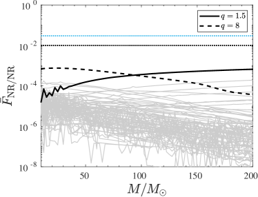
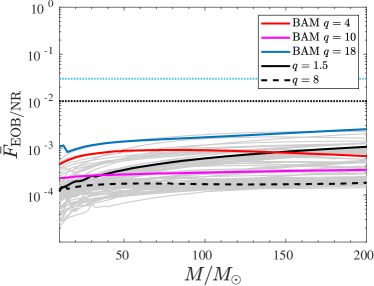
Figure 20: Nonspinning sector. Left panel: the NR/NR unfaithfulness between the highest and second highest resolutions available. Right panel: EOB/NR unfaithfulness for all available non-spinning datasets. The analytical waveforms are evaluated with $(\chi_{1},\chi_{2})=(0,10^{-4})$, so as to probe the stability of the model and its robustness in this regime.

Table 5: This table summarizes the SXS NR waveform data in the postpeak-calibration set, with mass-ratio $q=1$. From left to right, the columns report: the SXS simulation number, mass ratio and dimensionless spins $\chi_{i}$, and the maximum value of the unfaithfulness $\bar{F}$ between: The two highest resolutions of the NR dataset, if available, see Fig.2, and between EOB and NR, see Fig. 4.

#	id	$(q,\chi_{1},\chi_{2})$	$\bar{F}^{\rm max}_{\rm NR/NR}[\%]$	$\bar{F}^{\rm max}_{\rm EOB/NR}[\%]$
1	BBH:0178	$(1,+0.9942,+0.9942)$	$0.0066$	$0.0259$
2	BBH:0177	$(1,+0.9893,+0.9893)$	$0.0021$	$0.0345$
3	BBH:0172	$(1,+0.9794,+0.98)$	$0.0022$	$0.0188$
4	BBH:0157	$(1,+0.95,+0.95)$	$0.0027$	$0.0329$
5	BBH:0160	$(1,+0.9,+0.9)$	$0.0118$	$0.0114$
6	BBH:0153	$(1,+0.85,+0.85)$	..	$0.0249$
7	BBH:0230	$(1,+0.8,+0.8)$	$0.0016$	$0.0737$
8	BBH:0228	$(1,+0.6,+0.6)$	$0.0080$	$0.1458$
9	BBH:0150	$(1,+0.2,+0.2)$	$0.0027$	$0.0723$
10	BBH:0149	$(1,-0.2,-0.2)$	$0.0037$	$0.1369$
11	BBH:0148	$(1,-0.44,-0.44)$	$0.0013$	$0.0688$
12	BBH:0215	$(1,-0.6,-0.6)$	$0.0040$	$0.0903$
13	BBH:0154	$(1,-0.8,-0.8)$	$0.0036$	$0.0836$
14	BBH:0212	$(1,-0.8,-0.8)$	$0.0032$	$0.0610$
15	BBH:0159	$(1,-0.9,-0.9)$	$0.0069$	$0.0295$
16	BBH:0156	$(1,-0.95,-0.95)$	$0.0055$	$0.0798$
17	BBH:0231	$(1,+0.9,0)$	$0.0046$	$0.1094$
18	BBH:0232	$(1,+0.9,+0.5)$	$0.0073$	$0.0430$
19	BBH:0229	$(1,+0.65,+0.25)$	$0.0053$	$0.1411$
20	BBH:0227	$(1,+0.6,0)$	$0.0052$	$0.1776$
21	BBH:0005	$(1,+0.5,0)$	$0.0592$	$0.1396$
22	BBH:0226	$(1,-0.9,+0.5)$	$0.0018$	$0.0679$
23	BBH:0224	$(1,-0.8,+0.4)$	$0.0020$	$0.0842$
24	BBH:0225	$(1,+0.8,+0.4)$	$0.0014$	$0.0784$
25	BBH:0223	$(1,+0.3,0)$	$0.1520$	$0.1071$
26	BBH:0222	$(1,-0.3,0)$	$0.1598$	$0.0616$
27	BBH:0220	$(1,-0.8,-0.4)$	$0.0040$	$0.1042$
28	BBH:0221	$(1,+0.8,-0.4)$	$0.0053$	$0.1238$
29	BBH:0004	$(1,-0.5,0)$	$0.0189$	$0.0998$
30	BBH:0218	$(1,+0.5,-0.5)$	$0.2160$	$0.1794$
31	BBH:0219	$(1,+0.9,-0.5)$	$0.0076$	$0.1173$
32	BBH:0216	$(1,-0.6,0)$	$0.0040$	$0.0797$
33	BBH:0217	$(1,-0.6,+0.6)$	$0.0048$	$0.1103$
34	BBH:0214	$(1,-0.62,-0.25)$	$0.0010$	$0.0621$
35	BBH:0213	$(1,-0.8,+0.8)$	$0.0040$	$0.0938$
36	BBH:0209	$(1,-0.9,-0.5)$	$0.0010$	$0.0610$
37	BBH:0210	$(1,-0.9,0)$	$0.0024$	$0.0708$
38	BBH:0211	$(1,-0.9,+0.9)$	$0.0027$	$0.0918$

Table 6: This table summarizes the SXS NR waveform data in the postpeak-calibration set, with mass-ratio $1<q\leq 2$. From left to right, the columns report: the SXS simulation number, mass ratio and dimensionless spins $\chi_{i}$, and the maximum value of the unfaithfulness $\bar{F}$ between: The two highest resolutions of the NR dataset, if available, see Fig.2, and between EOB and NR, see Fig. 4.

#	id	$(q,\chi_{1},\chi_{2})$	$\bar{F}^{\rm max}_{\rm NR/NR}[\%]$	$\bar{F}^{\rm max}_{\rm EOB/NR}[\%]$
39	BBH:0306	$(1.3,+0.96,-0.9)$	$0.0031$	$0.2059$
40	BBH:0013	$(1.5,+0.5,0)$	..	$0.1420$
41	BBH:0025	$(1.5,+0.5,-0.5)$	$0.0278$	$0.2446$
42	BBH:0016	$(1.5,-0.5,0)$	$0.0009$	$0.0262$
43	BBH:0019	$(1.5,-0.5,+0.5)$	$0.0213$	$0.0408$
44	BBH:0258	$(2,+0.87,-0.85)$	$0.0061$	$0.2599$
45	BBH:0257	$(2,+0.85,+0.85)$	$0.0024$	$0.4144$
46	BBH:0254	$(2,+0.6,-0.6)$	$0.0009$	$0.2218$
47	BBH:0255	$(2,+0.6,0)$	$0.0023$	$0.1324$
48	BBH:0256	$(2,+0.6,+0.6)$	$0.0068$	$0.0771$
49	BBH:0253	$(2,+0.5,+0.5)$	$0.0040$	$0.0844$
50	BBH:0252	$(2,+0.37,-0.85)$	$0.0029$	$0.1659$
51	BBH:0249	$(2,+0.3,-0.3)$	$0.0057$	$0.0888$
52	BBH:0250	$(2,+0.3,0)$	$0.0045$	$0.0837$
53	BBH:0251	$(2,+0.3,+0.3)$	$0.0037$	$0.0755$
54	BBH:0248	$(2,+0.13,+0.85)$	$0.0030$	$0.0666$
55	BBH:0244	$(2,0,-0.6)$	$0.0010$	$0.0542$
56	BBH:0245	$(2,0,-0.3)$	$0.0226$	$0.0385$
57	BBH:0246	$(2,0,+0.3)$	$0.0081$	$0.0395$
58	BBH:0247	$(2,0,+0.6)$	$0.0041$	$0.0440$
59	BBH:0243	$(2,-0.13,-0.85)$	$0.0006$	$0.0538$
60	BBH:0240	$(2,-0.3,-0.3)$	$0.0614$	$0.0235$
61	BBH:0241	$(2,-0.3,0)$	$0.0129$	$0.0251$
62	BBH:0242	$(2,-0.3,+0.3)$	$0.0260$	$0.0282$
63	BBH:0239	$(2,-0.37,+0.85)$	$0.0005$	$0.0338$
64	BBH:0238	$(2,-0.5,-0.5)$	$0.1110$	$0.0351$
65	BBH:0235	$(2,-0.6,-0.6)$	$0.0048$	$0.0267$
66	BBH:0236	$(2,-0.6,0)$	$0.0029$	$0.0483$
67	BBH:0237	$(2,-0.6,+0.6)$	$0.0014$	$0.0880$
68	BBH:0234	$(2,-0.85,-0.85)$	$0.0049$	$0.0709$
69	BBH:0233	$(2,-0.87,+0.85)$	$0.0012$	$0.1564$

Table 7: This table summarizes the SXS NR waveform data in the postpeak-calibration set, with mass-ratio $3\leq q$. From left to right, the columns report: the SXS simulation number, mass ratio and dimensionless spins spins $\chi_{i}$, and the maximum value of the unfaithfulness $\bar{F}$ between: The two highest resolutions of the NR dataset, if available, see Fig.2, and between EOB and NR, see Fig. 4.

#	id	$(q,\chi_{1},\chi_{2})$	$\bar{F}^{\rm max}_{\rm NR/NR}[\%]$	$\bar{F}^{\rm max}_{\rm EOB/NR}[\%]$
70	BBH:0036	$(3,-0.5,0)$	$0.0010$	$0.0405$
71	BBH:0045	$(3,+0.5,-0.5)$	..	$0.1456$
72	BBH:0174	$(3,+0.5,0)$	$0.1040$	$0.1828$
73	BBH:0260	$(3,-0.85,-0.85)$	$0.0004$	$0.0744$
74	BBH:0261	$(3,-0.73,+0.85)$	$0.0016$	$0.1453$
75	BBH:0262	$(3,-0.6,0)$	$0.0002$	$0.0362$
76	BBH:0263	$(3,-0.6,+0.6)$	$0.0009$	$0.0914$
77	BBH:0264	$(3,-0.6,-0.6)$	$0.0024$	$0.0449$
78	BBH:0265	$(3,-0.6,-0.4)$	$0.0008$	$0.0329$
79	BBH:0266	$(3,-0.6,+0.4)$	$0.0003$	$0.0714$
80	BBH:0267	$(3,-0.5,-0.5)$	$0.0058$	$0.0368$
81	BBH:0268	$(3,-0.4,-0.6)$	$0.0016$	$0.0249$
82	BBH:0269	$(3,-0.4,+0.6)$	$0.0017$	$0.0516$
83	BBH:0270	$(3,-0.3,-0.3)$	$0.0038$	$0.0217$
84	BBH:0271	$(3,-0.3,0)$	$0.0014$	$0.0255$
85	BBH:0272	$(3,-0.3,+0.3)$	$0.0035$	$0.0291$
86	BBH:0273	$(3,-0.27,-0.85)$	$0.0027$	$0.0605$
87	BBH:0274	$(3,-0.23,+0.85)$	$0.0018$	$0.0355$
88	BBH:0275	$(3,0,-0.6)$	$0.0008$	$0.0602$
89	BBH:0276	$(3,0,-0.3)$	$0.0028$	$0.0373$
90	BBH:0277	$(3,0,+0.3)$	$0.0029$	$0.0194$
91	BBH:0278	$(3,0,+0.6)$	$0.0015$	$0.0252$
92	BBH:0279	$(3,+0.23,-0.85)$	$0.0010$	$0.0670$
93	BBH:0280	$(3,+0.27,+0.85)$	$0.0052$	$0.0405$
94	BBH:0281	$(3,+0.3,-0.3)$	$0.0027$	$0.0729$
95	BBH:0282	$(3,+0.3,0)$	$0.0011$	$0.0223$
96	BBH:0283	$(3,+0.3,+0.3)$	$0.0032$	$0.0328$
97	BBH:0284	$(3,+0.4,-0.6)$	$0.0005$	$0.1288$
98	BBH:0285	$(3,+0.4,+0.6)$	$0.0013$	$0.0257$
99	BBH:0286	$(3,+0.5,+0.5)$	$0.0022$	$0.0257$
100	BBH:0287	$(3,+0.6,-0.6)$	$0.0053$	$0.1954$
101	BBH:0288	$(3,+0.6,-0.4)$	$0.0006$	$0.0683$
102	BBH:0289	$(3,+0.6,0)$	$0.0005$	$0.0624$
103	BBH:0290	$(3,+0.6,+0.4)$	$0.0032$	$0.0260$
104	BBH:0291	$(3,+0.6,+0.6)$	$0.0010$	$0.0129$
105	BBH:0292	$(3,+0.73,-0.85)$	$0.0009$	$0.3817$
106	BBH:0293	$(3,+0.85,+0.85)$	$0.0046$	$0.4764$
107	BBH:0060	$(5,-0.5,0)$	..	$0.0217$
108	BBH:0110	$(5,+0.5,0)$	..	$0.0383$
109	BBH:0208	$(5,-0.9,0)$	$0.0385$	$0.0667$
110	BBH:0202	$(7,+0.6,0)$	$0.0048$	$0.3976$
111	BBH:0203	$(7,+0.4,0)$	$0.0095$	$0.0556$
112	BBH:0205	$(7,-0.4,0)$	$0.0040$	$0.0484$
113	BBH:0207	$(7,-0.6,0)$	$0.0011$	$0.0613$
114	BBH:0064	$(8,-0.5,0)$	$0.0338$	$0.0325$
115	BBH:0065	$(8,+0.5,0)$	$0.0189$	$0.1440$
116	BBH:1375	$(8,-0.9,0)$	..	$0.1223$

Table 8: This table summarizes the BAM NR waveform data in the postpeak-calibration set. From left to right, the columns report: the simulation number, mass ratio and dimensionless spins spins $\chi_{i}$, and the maximum value of the EOB/NR unfaithfulness $\bar{F}$, see Fig. 4. These waveforms were mostly presented in Refs. Husa et al. (2016); Khan et al. (2016); Keitel et al. (2017)

	#	$(q,\chi_{1},\chi_{2})$	$\bar{F}^{\rm max}_{\rm EOB/NR}[\%]$
	117	$(2,+0.5,+0.5)$	$0.3458$
	118	$(2,+0.75,+0.75)$	$0.4149$
	119	$(3,-0.5,-0.5)$	$0.1895$
	120	$(4,-0.75,-0.75)$	$0.2898$
	121	$(4,-0.5,-0.5)$	$0.1588$
	122	$(4,-0.25,-0.25)$	$0.1096$
	123	$(4,+0.25,+0.25)$	$0.0402$
	124	$(4,+0.5,+0.5)$	$0.0385$
	125	$(4,+0.75,+0.75)$	$0.0378$
	126	$(8,-0.85,-0.85)$	$0.0791$
	127	$(8,+0.8,0)$	$0.2555$
	128	$(8,+0.85,+0.85)$	$0.2530$
	129	$(18,-0.8,0)$	$0.1653$
	130	$(18,-0.4,0)$	$0.0418$
	131	$(18,+0.4,0)$	$0.0232$
	132	$(18,+0.8,0)$	$0.1029$

Table 9: This table summarizes part of the SXS NR waveform data in the validation set with $q=1$. From left to right, the columns report: the SXS simulation number, mass ratio and dimensionless spins spins $\chi_{i}$, and the maximum value of the unfaithfulness $\bar{F}$ between: The two highest resolutions of the NR dataset, if available, see Fig.2, and between EOB and NR, see Fig. 4.

#	id	$(q,\chi_{1},\chi_{2})$	$\bar{F}^{\rm max}_{\rm NR/NR}[\%]$	$\bar{F}^{\rm max}_{\rm EOB/NR}[\%]$
133	BBH:1124	$(1,+0.9980,+0.9980)$	..	$0.0800$
134	BBH:0158	$(1,+0.97,+0.97)$	$0.0031$	$0.0510$
135	BBH:0176	$(1,+0.96,+0.96)$	$0.0065$	$0.0264$
136	BBH:0155	$(1,+0.8,+0.8)$	$0.0035$	$0.0749$
137	BBH:1477	$(1,+0.8,+0.8)$	$0.0037$	$0.0743$
138	BBH:0328	$(1,+0.8,+0.8)$	$0.0034$	$0.0733$
139	BBH:2104	$(1,+0.8,+0.8)$	$0.0033$	$0.0742$
140	BBH:1481	$(1,+0.8,+0.73)$	$0.0032$	$0.0839$
141	BBH:0175	$(1,+0.75,+0.75)$	$0.0030$	$0.0964$
142	BBH:2106	$(1,+0.9,+0.5)$	$0.0064$	$0.0441$
143	BBH:1497	$(1,+0.68,+0.67)$	$0.0032$	$0.1165$
144	BBH:1495	$(1,+0.78,+0.53)$	$0.0058$	$0.0698$
145	BBH:0152	$(1,+0.6,+0.6)$	$0.0047$	$0.1483$
146	BBH:2099	$(1,+0.8,+0.4)$	$0.0048$	$0.0790$
147	BBH:2102	$(1,+0.6,+0.6)$	$0.0007$	$0.1469$
148	BBH:1123	$(1,+0.5,+0.5)$	$0.0033$	$0.1899$
149	BBH:0394	$(1,+0.6,+0.4)$	$0.0023$	$0.0936$
150	BBH:2103	$(1,+0.65,+0.25)$	$0.0022$	$0.3458$
151	BBH:2105	$(1,+0.9,0)$	$0.0002$	$0.0652$
152	BBH:1122	$(1,+0.44,+0.44)$	$0.0031$	$0.2051$
153	BBH:1503	$(1,+0.73,+0.14)$	$0.0028$	$0.1642$
154	BBH:1501	$(1,+0.75,+0.1)$	$0.0040$	$0.1363$
155	BBH:0326	$(1,+0.8,0)$	$0.0056$	$0.1324$
156	BBH:1507	$(1,+0.5,+0.3)$	$0.0032$	$0.1965$
157	BBH:1376	$(1,+0.25,+0.5)$	$0.0035$	$0.2068$
158	BBH:2101	$(1,+0.6,0)$	$0.0039$	$0.1777$
159	BBH:0418	$(1,+0.4,0)$	$0.0041$	$0.1332$
160	BBH:2095	$(1,+0.8,-0.4)$	$0.0006$	$0.1245$
161	BBH:2093	$(1,+0.9,-0.5)$	$0.0018$	$0.1189$
162	BBH:2097	$(1,+0.3,0)$	$0.0014$	$0.3091$
163	BBH:1502	$(1,+0.7,-0.4)$	$0.0026$	$0.0786$
164	BBH:0366	$(1,+0.2,0)$	$0.0027$	$0.1055$
165	BBH:1114	$(1,+0.2,0)$	..	$0.1452$
166	BBH:0370	$(1,+0.4,-0.2)$	$0.0006$	$0.4640$
167	BBH:0376	$(1,+0.6,-0.4)$	$0.0013$	$0.4585$
168	BBH:1506	$(1,+0.46,-0.3)$	$0.0023$	$0.1897$
169	BBH:1476	$(1,-0.8,+0.8)$	$0.0045$	$0.0926$
170	BBH:2085	$(1,-0.9,+0.9)$	$0.0021$	$0.0910$
171	BBH:2087	$(1,-0.8,+0.8)$	$0.0007$	$0.0932$
172	BBH:0304	$(1,-0.5,+0.5)$	$0.0014$	$0.2308$
173	BBH:2091	$(1,-0.6,+0.6)$	$0.0019$	$0.3086$
174	BBH:2092	$(1,+0.5,-0.5)$	$0.0028$	$0.3435$
175	BBH:0327	$(1,-0.8,+0.8)$	$0.0042$	$0.0457$
176	BBH:0330	$(1,-0.8,+0.8)$	$0.0005$	$0.0930$
177	BBH:0459	$(1,-0.4,+0.2)$	$0.0023$	$0.0359$
178	BBH:0447	$(1,-0.6,+0.4)$	$0.0054$	$0.2526$
179	BBH:1351	$(1,-0.23,0)$	$0.0005$	$0.0813$
180	BBH:2096	$(1,-0.3,0)$	$0.0005$	$0.1127$
181	BBH:1509	$(1,-0.24,-0.1)$	$0.0014$	$0.2097$
182	BBH:2100	$(1,-0.9,+0.5)$	$0.0017$	$0.0481$
183	BBH:2098	$(1,-0.8,+0.4)$	$0.0044$	$0.0475$

Table 10: This table continues to summarizes the SXS NR waveform data in the validation set, with mass-ratios $1\leq q\leq 1.2$. From left to right, the columns report: the SXS simulation number, mass ratio and dimensionless spins spins $\chi_{i}$, and the maximum value of the unfaithfulness $\bar{F}$ between: The two highest resolutions of the NR dataset, if available, see Fig.2, and between EOB and NR, see Fig. 4.

#	id	$(q,\chi_{1},\chi_{2})$	$\bar{F}^{\rm max}_{\rm NR/NR}[\%]$	$\bar{F}^{\rm max}_{\rm EOB/NR}[\%]$
184	BBH:0415	$(1,-0.4,0)$	$0.0021$	$0.1571$
185	BBH:1499	$(1,-0.75,+0.34)$	$0.0021$	$0.0440$
186	BBH:1498	$(1,+0.22,-0.8)$	$0.0093$	$0.0261$
187	BBH:2090	$(1,-0.6,0)$	$0.0036$	$0.0464$
188	BBH:0436	$(1,-0.4,-0.2)$	$0.0019$	$0.1467$
189	BBH:0585	$(1,-0.6,0)$	$0.0009$	$0.0863$
190	BBH:0325	$(1,-0.8,0)$	$0.0022$	$0.1511$
191	BBH:1134	$(1,-0.44,-0.44)$	$0.0025$	$0.0383$
192	BBH:1135	$(1,-0.44,-0.44)$	$0.0047$	$0.0265$
193	BBH:2088	$(1,-0.62,-0.25)$	$0.0016$	$0.1088$
194	BBH:1144	$(1,-0.44,-0.44)$	$0.0054$	$0.0393$
195	BBH:2084	$(1,-0.9,0)$	$0.0031$	$0.1176$
196	BBH:1500	$(1,-0.77,-0.2)$	$0.0012$	$0.0560$
197	BBH:0462	$(1,-0.6,-0.4)$	$0.0025$	$0.0454$
198	BBH:0151	$(1,-0.6,-0.6)$	$0.0022$	$0.1071$
199	BBH:2094	$(1,-0.8,-0.4)$	$0.0009$	$0.0999$
200	BBH:2089	$(1,-0.6,-0.6)$	$0.0072$	$0.0900$
201	BBH:1492	$(1,-0.8,-0.47)$	$0.0009$	$0.0756$
202	BBH:2083	$(1,-0.9,-0.5)$	$0.0067$	$0.0565$
203	BBH:1475	$(1,-0.8,-0.8)$	$0.0026$	$0.0468$
204	BBH:2086	$(1,-0.8,-0.8)$	$0.0033$	$0.0349$
205	BBH:0329	$(1,-0.8,-0.8)$	$0.0020$	$0.0509$
206	BBH:1137	$(1,-0.97,-0.97)$	$0.0021$	$0.1300$
207	BBH:0544	$(1,0,+0.7)$	$0.0021$	$0.2125$
208	BBH:0518	$(1.1,-0.14,+0.43)$	$0.0012$	$0.1204$
209	BBH:1513	$(1.1,-0.1,0)$	$0.0051$	$0.1661$
210	BBH:0409	$(1.2,+0.4,+0.8)$	$0.0058$	$0.1314$
211	BBH:1490	$(1.2,+0.41,+0.76)$	$0.0026$	$0.1835$
212	BBH:1496	$(1.2,+0.8,+0.03)$	$0.0008$	$0.1548$
213	BBH:0311	$(1.2,+0.42,+0.38)$	$0.0019$	$0.2521$
214	BBH:0486	$(1.2,0,+0.8)$	$0.0024$	$0.1712$
215	BBH:0559	$(1.2,-0.2,+0.8)$	$0.0035$	$0.0903$
216	BBH:0475	$(1.2,-0.4,+0.8)$	$0.0036$	$0.0776$
217	BBH:1352	$(1.2,+0.71,-0.67)$	$0.0013$	$0.1645$
218	BBH:0503	$(1.2,-0.6,+0.8)$	$0.0017$	$0.0343$
219	BBH:0312	$(1.2,+0.4,-0.48)$	$0.0046$	$0.1594$
220	BBH:1353	$(1.2,+0.33,-0.44)$	$0.0013$	$0.3409$
221	BBH:0309	$(1.2,+0.33,-0.44)$	$0.0103$	$0.2187$
222	BBH:0305	$(1.2,+0.33,-0.44)$	$0.0015$	$0.1682$
223	BBH:0318	$(1.2,+0.33,-0.44)$	$0.0018$	$0.2182$
224	BBH:0319	$(1.2,+0.33,-0.44)$	$0.0096$	$0.1225$
225	BBH:0313	$(1.2,+0.38,-0.5)$	$0.0035$	$0.2190$
226	BBH:0465	$(1.2,+0.6,-0.8)$	$0.0010$	$0.1743$
227	BBH:0314	$(1.2,+0.31,-0.46)$	$0.0021$	$0.2401$
228	BBH:0307	$(1.2,+0.32,-0.58)$	$0.0016$	$0.1026$
229	BBH:0626	$(1.2,-0.83,+0.73)$	$0.0061$	$0.0217$
230	BBH:0535	$(1.2,+0.2,-0.8)$	$0.0023$	$0.0812$
231	BBH:0523	$(1.2,-0.2,-0.47)$	$0.0012$	$0.0362$
232	BBH:0398	$(1.2,0,-0.8)$	$0.0036$	$0.0475$
233	BBH:0386	$(1.2,-0.2,-0.8)$	$0.0012$	$0.1080$
234	BBH:0438	$(1.2,-0.6,-0.8)$	$0.0021$	$0.0363$

Table 11: This table summarizes the SXS NR waveform data in the validation set, with mass-ratios $1.3\leq q\leq 1.7$. From left to right, the columns report: the SXS simulation number, mass ratio and dimensionless spins $\chi_{i}$, and the maximum value of the unfaithfulness $\bar{F}$ between: The two highest resolutions of the NR dataset, if available, see Fig.2, and between EOB and NR, see Fig. 4.

#	id	$(q,\chi_{1},\chi_{2})$	$\bar{F}^{\rm max}_{\rm NR/NR}[\%]$	$\bar{F}^{\rm max}_{\rm EOB/NR}[\%]$
235	BBH:0507	$(1.3,+0.8,+0.4)$	$0.0043$	$0.1326$
236	BBH:1493	$(1.3,0,+0.8)$	$0.0029$	$0.1639$
237	BBH:0525	$(1.3,+0.8,-0.4)$	$0.0008$	$0.1835$
238	BBH:1505	$(1.3,-0.1,+0.55)$	$0.0021$	$0.1400$
239	BBH:0591	$(1.2,0,+0.4)$	$0.0028$	$0.0926$
240	BBH:1508	$(1.3,+0.3,-0.07)$	$0.0057$	$0.1296$
241	BBH:1474	$(1.3,+0.72,-0.8)$	$0.0025$	$0.2317$
242	BBH:1223	$(1.2,+0.38,-0.46)$	$0.0034$	$0.1685$
243	BBH:0651	$(1.3,0,+0.03)$	$0.0051$	$0.1191$
244	BBH:0650	$(1.3,0,+0.03)$	$0.0141$	$0.3692$
245	BBH:0315	$(1.3,+0.32,-0.56)$	$0.0011$	$0.3037$
246	BBH:0464	$(1.2,0,-0.4)$	$0.0013$	$0.1014$
247	BBH:1487	$(1.3,-0.8,+0.5)$	$0.0022$	$0.0636$
248	BBH:0377	$(1.3,-0.8,+0.4)$	$0.0017$	$0.0739$
249	BBH:0466	$(1.3,-0.8,-0.4)$	$0.0006$	$0.0388$
250	BBH:1471	$(1.3,-0.78,-0.8)$	$0.0009$	$0.0561$
251	BBH:0129	$(1.4,+0.09,-0.07)$	..	$0.1464$
252	BBH:1482	$(1.4,-0.58,+0.8)$	$0.0016$	$0.0301$
253	BBH:0625	$(1.4,-0.71,+0.22)$	$0.0046$	$0.0519$
254	BBH:1146	$(1.5,+0.95,+0.95)$	$0.0446$	$0.8427$
255	BBH:1473	$(1.4,+0.7,+0.8)$	$0.0060$	$0.1843$
256	BBH:0441	$(1.5,+0.6,+0.8)$	$0.0034$	$0.1585$
257	BBH:0385	$(1.5,+0.8,0)$	$0.0016$	$0.1737$
258	BBH:0361	$(1.5,0,+0.8)$	$0.0025$	$0.1085$
259	BBH:0372	$(1.5,+0.8,-0.4)$	$0.0025$	$0.1282$
260	BBH:0499	$(1.5,+0.01,+0.74)$	$0.0041$	$0.1005$
261	BBH:0009	$(1.5,+0.5,0)$	..	$0.2536$
262	BBH:0392	$(1.5,-0.2,+0.8)$	$0.0024$	$0.0555$
263	BBH:0440	$(1.5,0,+0.4)$	$0.0014$	$0.0512$
264	BBH:0369	$(1.5,+0.6,-0.8)$	$0.0026$	$0.3375$
265	BBH:1511	$(1.5,+0.03,-0.1)$	$0.0024$	$0.0952$
266	BBH:0579	$(1.5,+0.4,-0.8)$	$0.0022$	$0.0881$
267	BBH:0012	$(1.5,-0.5,0)$	$0.0068$	$0.0341$
268	BBH:0014	$(1.5,-0.5,0)$	$0.0561$	$0.0425$
269	BBH:0101	$(1.5,-0.5,0)$	..	$0.0284$
270	BBH:0404	$(1.5,0,-0.8)$	$0.0032$	$0.0962$
271	BBH:0437	$(1.5,-0.2,-0.8)$	$0.0019$	$0.0552$
272	BBH:1480	$(1.5,-0.8,-0.3)$	$0.0035$	$0.0304$
273	BBH:0397	$(1.5,-0.8,-0.4)$	$0.0017$	$0.0419$
274	BBH:1470	$(1.5,-0.73,-0.8)$	$0.0035$	$0.0345$
275	BBH:0519	$(1.6,+0.64,+0.4)$	$0.0048$	$0.0812$
276	BBH:1488	$(1.6,-0.33,+0.75)$	$0.0061$	$0.0357$
277	BBH:1479	$(1.6,-0.56,-0.8)$	$0.0016$	$0.0380$
278	BBH:0501	$(1.7,+0.6,+0.8)$	$0.0063$	$0.1260$
279	BBH:0435	$(1.7,+0.4,+0.8)$	$0.0029$	$0.0817$
280	BBH:0566	$(1.7,+0.2,+0.8)$	$0.0041$	$0.0971$
281	BBH:0382	$(1.7,0,+0.8)$	$0.0017$	$0.0701$
282	BBH:0529	$(1.7,0,+0.53)$	$0.0035$	$0.0627$
283	BBH:0550	$(1.7,-0.2,+0.8)$	$0.0021$	$0.0534$
284	BBH:0451	$(1.7,0,+0.4)$	$0.0022$	$0.0526$
285	BBH:0488	$(1.7,+0.6,-0.8)$	$0.0040$	$0.2618$

Table 12: This table continues to summarizes the SXS NR waveform data in the validation set, with mass-ratios $1.7\leq q\leq 2$. From left to right, the columns report: the SXS simulation number, mass ratio and dimensionless spins $\chi_{i}$, and the maximum value of the unfaithfulness $\bar{F}$ between: The two highest resolutions of the NR dataset, if available, see Fig.2, and between EOB and NR, see Fig. 4.

#	id	$(q,\chi_{1},\chi_{2})$	$\bar{F}^{\rm max}_{\rm NR/NR}[\%]$	$\bar{F}^{\rm max}_{\rm EOB/NR}[\%]$
286	BBH:0678	$(1.7,0,+0.03)$	$0.0073$	$0.1337$
287	BBH:0677	$(1.7,0,+0.03)$	$0.0037$	$0.1791$
288	BBH:0676	$(1.7,0,+0.02)$	$0.0050$	$0.3450$
289	BBH:0355	$(1.7,-0.6,+0.8)$	$0.0015$	$0.0550$
290	BBH:1491	$(1.7,+0.2,-0.7)$	$0.0020$	$0.0999$
291	BBH:0473	$(1.7,+0.2,-0.8)$	$0.0019$	$0.0876$
292	BBH:1465	$(1.7,-0.79,+0.77)$	$0.0038$	$0.0740$
293	BBH:0510	$(1.7,-0.02,-0.75)$	$0.0044$	$0.0639$
294	BBH:0423	$(1.7,0,-0.8)$	$0.0008$	$0.0577$
295	BBH:0402	$(1.7,-0.8,+0.4)$	$0.0017$	$0.0725$
296	BBH:0414	$(1.7,-0.4,-0.8)$	$0.0038$	$0.0438$
297	BBH:0512	$(1.7,-0.6,-0.8)$	$0.0006$	$0.0476$
298	BBH:0388	$(1.8,+0.8,+0.4)$	$0.0034$	$0.1265$
299	BBH:0552	$(1.8,+0.8,-0.4)$	$0.0016$	$0.2418$
300	BBH:1510	$(1.8,+0.03,+0.3)$	$0.0018$	$0.0549$
301	BBH:0371	$(1.8,0,-0.4)$	$0.0060$	$0.0532$
302	BBH:0545	$(1.8,0,-0.8)$	$0.0026$	$0.0306$
303	BBH:0454	$(1.8,-0.8,-0.4)$	$0.0011$	$0.0203$
304	BBH:1469	$(1.9,+0.8,+0.67)$	$0.0042$	$0.1686$
305	BBH:0530	$(2,0,+0.54)$	$0.0015$	$0.0449$
306	BBH:1466	$(1.9,+0.7,-0.8)$	$0.0015$	$0.2468$
307	BBH:0555	$(1.9,0,+0.53)$	$0.0008$	$0.0483$
308	BBH:0368	$(2,-0.05,+0.25)$	$0.0015$	$0.0351$
309	BBH:0403	$(1.9,0,-0.05)$	$0.0048$	$0.0442$
310	BBH:0580	$(2,+0.02,-0.8)$	$0.0020$	$0.0756$
311	BBH:2131	$(2,+0.85,+0.85)$	$0.0011$	$0.3993$
312	BBH:0333	$(2,+0.8,+0.8)$	$0.0115$	$0.2591$
313	BBH:2130	$(2,+0.6,+0.6)$	$0.0032$	$0.0779$
314	BBH:1478	$(2,+0.8,+0.13)$	$0.0047$	$0.1406$
315	BBH:2127	$(2,+0.5,+0.5)$	$0.0102$	$0.0819$
316	BBH:1148	$(2,+0.43,+0.5)$	$0.0048$	$0.0890$
317	BBH:0410	$(2,+0.6,0)$	$0.0047$	$0.2876$
318	BBH:0574	$(2,+0.4,+0.4)$	$0.0016$	$0.1062$
319	BBH:2129	$(2,+0.6,0)$	$0.0016$	$0.1325$
320	BBH:2122	$(2,+0.13,+0.85)$	$0.0022$	$0.0672$
321	BBH:2125	$(2,+0.3,+0.3)$	$0.0017$	$0.0784$
322	BBH:2132	$(2,+0.87,-0.85)$	$0.0039$	$0.4141$
323	BBH:0399	$(2,+0.2,+0.4)$	$0.0013$	$0.0681$
324	BBH:0332	$(2,0,+0.8)$	$0.0021$	$0.0495$
325	BBH:0513	$(2,+0.6,-0.4)$	$0.0030$	$0.1416$
326	BBH:2128	$(2,+0.6,-0.6)$	$0.0051$	$0.1713$
327	BBH:2121	$(2,0,+0.6)$	$0.0017$	$0.0426$
328	BBH:2124	$(2,+0.3,0)$	$0.0014$	$0.0793$
329	BBH:0903	$(2,0,+0.6)$	$0.0009$	$0.0697$
330	BBH:0893	$(2,0,+0.58)$	$0.0020$	$0.0621$
331	BBH:0885	$(2,0,+0.57)$	$0.0024$	$0.1064$
332	BBH:1504	$(2,+0.25,+0.08)$	$0.0013$	$0.0726$
333	BBH:0448	$(2,+0.4,-0.4)$	$0.0031$	$0.1224$
334	BBH:0407	$(2,0,+0.4)$	$0.0020$	$0.0394$
335	BBH:0599	$(2,+0.2,0)$	$0.0027$	$0.0698$
336	BBH:1147	$(2,+0.43,-0.5)$	$0.0094$	$0.1338$

Table 13: This table continues to summarizes the SXS NR waveform data in the validation set, with mass-ratios $2\leq q\leq 2.6$. From left to right, the columns report: the SXS simulation number, mass ratio and dimensionless spins $\chi_{i}$, and the maximum value of the unfaithfulness $\bar{F}$ between: The two highest resolutions of the NR dataset, if available, see Fig.2, and between EOB and NR, see Fig. 4.

#	id	$(q,\chi_{1},\chi_{2})$	$\bar{F}^{\rm max}_{\rm NR/NR}[\%]$	$\bar{F}^{\rm max}_{\rm EOB/NR}[\%]$
337	BBH:2120	$(2,0,+0.3)$	$0.0013$	$0.0368$
338	BBH:2123	$(2,+0.3,-0.3)$	$0.0021$	$0.1055$
339	BBH:2113	$(2,-0.37,+0.85)$	$0.0012$	$0.0344$
340	BBH:0913	$(2,0,+0.03)$	$0.0034$	$0.0802$
341	BBH:0971	$(2,0,+0.03)$	$0.0010$	$0.0460$
342	BBH:0987	$(2,0,+0.03)$	$0.0080$	$0.0745$
343	BBH:0703	$(2,0,+0.03)$	$0.0085$	$0.1011$
344	BBH:0704	$(2,0,+0.03)$	$0.0007$	$0.0949$
345	BBH:0921	$(2,0,+0.03)$	$0.0021$	$0.1244$
346	BBH:0702	$(2,0,+0.02)$	$0.0038$	$0.2062$
347	BBH:0961	$(2,0,+0.02)$	$0.0011$	$0.1312$
348	BBH:0979	$(2,0,+0.02)$	$0.0068$	$0.2057$
349	BBH:0931	$(2,0,+0.0)$	$0.0034$	$0.1406$
350	BBH:0554	$(2,+0.2,-0.4)$	$0.0029$	$0.0954$
351	BBH:0354	$(2,-0.2,+0.4)$	$0.0006$	$0.0234$
352	BBH:2126	$(2,+0.37,-0.85)$	$0.0031$	$0.1498$
353	BBH:0482	$(2,-0.02,-0.13)$	$0.0040$	$0.0409$
354	BBH:2119	$(2,0,-0.3)$	$0.0034$	$0.0466$
355	BBH:2116	$(2,-0.3,+0.3)$	$0.0027$	$0.0208$
356	BBH:1112	$(2,-0.2,0)$	..	$0.0227$
357	BBH:0375	$(2,0,-0.4)$	$0.0013$	$0.0204$
358	BBH:0954	$(2,0,-0.56)$	$0.0031$	$0.0784$
359	BBH:0947	$(2,0,-0.56)$	$0.0056$	$0.1312$
360	BBH:0940	$(2,0,-0.57)$	$0.0040$	$0.1698$
361	BBH:2118	$(2,0,-0.6)$	$0.0025$	$0.0617$
362	BBH:2111	$(2,-0.6,+0.6)$	$0.0017$	$0.0882$
363	BBH:2115	$(2,-0.3,0)$	$0.0038$	$0.0223$
364	BBH:0331	$(2,0,-0.8)$	$0.0075$	$0.0668$
365	BBH:0412	$(2,-0.2,-0.4)$	$0.0018$	$0.0295$
366	BBH:0335	$(2,-0.8,+0.8)$	$0.0012$	$0.1186$
367	BBH:2107	$(2,-0.87,+0.85)$	$0.0012$	$0.1700$
368	BBH:2114	$(2,-0.3,-0.3)$	$0.0021$	$0.0234$
369	BBH:2117	$(2,-0.13,-0.85)$	$0.0057$	$0.0642$
370	BBH:2110	$(2,-0.6,0)$	$0.0021$	$0.0435$
371	BBH:0584	$(2,-0.4,-0.4)$	$0.0027$	$0.0260$
372	BBH:0461	$(2,-0.6,0)$	$0.0018$	$0.0318$
373	BBH:2112	$(2,-0.5,-0.5)$	$0.0031$	$0.0256$
374	BBH:0387	$(2,-0.6,-0.4)$	$0.0022$	$0.0239$
375	BBH:2109	$(2,-0.6,-0.6)$	$0.0015$	$0.0273$
376	BBH:0334	$(2,-0.8,-0.8)$	$0.0033$	$0.0519$
377	BBH:2108	$(2,-0.85,-0.85)$	$0.0068$	$0.0766$
378	BBH:1467	$(2.2,-0.56,+0.8)$	$0.0051$	$0.0538$
379	BBH:1494	$(2.2,-0.47,-0.4)$	$0.0025$	$0.0303$
380	BBH:1459	$(2.3,+0.76,+0.8)$	$0.0112$	$0.1404$
381	BBH:1468	$(2.3,+0.51,+0.8)$	$0.0068$	$0.0635$
382	BBH:0631	$(2.3,-0.13,-0.36)$	$0.0036$	$0.0161$
383	BBH:1453	$(2.4,+0.8,-0.8)$	$0.0048$	$0.1916$
384	BBH:1512	$(2.4,+0.24,0)$	$0.0045$	$0.0639$
385	BBH:1472	$(2.4,-0.8,-0.1)$	$0.0022$	$0.0243$
386	BBH:1454	$(2.5,-0.8,-0.73)$	$0.0030$	$0.0733$
387	BBH:1462	$(2.6,-0.8,+0.5)$	$0.0021$	$0.0714$

Table 14: This table summarizes the SXS NR waveform data in the validation set, with mass-ratios $2.9\leq q\leq 3$. From left to right, the columns report: the SXS simulation number, mass ratio and dimensionless spins $\chi_{i}$, and the maximum value of the unfaithfulness $\bar{F}$ between: The two highest resolutions of the NR dataset, if available, see Fig.2, and between EOB and NR, see Fig. 4.

#	id	$(q,\chi_{1},\chi_{2})$	$\bar{F}^{\rm max}_{\rm NR/NR}[\%]$	$\bar{F}^{\rm max}_{\rm EOB/NR}[\%]$
388	BBH:1461	$(2.9,-0.45,-0.8)$	$0.0044$	$0.0299$
389	BBH:1484	$(3,-0.56,+0.3)$	$0.0019$	$0.0399$
390	BBH:1456	$(3,+0.74,+0.7)$	$0.0123$	$0.0528$
391	BBH:1150	$(3,+0.7,+0.6)$	$0.0088$	$0.0176$
392	BBH:1151	$(3,+0.7,+0.6)$	$0.0093$	$0.0214$
393	BBH:1152	$(3,+0.7,+0.6)$	$0.0079$	$0.0214$
394	BBH:1382	$(3,+0.7,+0.6)$	$0.0072$	$0.0298$
395	BBH:2163	$(3,+0.6,+0.6)$	$0.0029$	$0.0135$
396	BBH:2162	$(3,+0.6,+0.4)$	$0.0020$	$0.0270$
397	BBH:2158	$(3,+0.5,+0.5)$	$0.0089$	$0.0201$
398	BBH:0047	$(3,+0.5,+0.5)$	..	$0.0212$
399	BBH:2161	$(3,+0.6,0)$	$0.0052$	$0.0673$
400	BBH:2157	$(3,+0.4,+0.6)$	$0.0043$	$0.0256$
401	BBH:2152	$(3,+0.27,+0.85)$	$0.0047$	$0.0392$
402	BBH:0031	$(3,+0.5,0)$	$0.0244$	$0.0679$
403	BBH:0041	$(3,+0.5,0)$	..	$0.0571$
404	BBH:2160	$(3,+0.6,-0.4)$	$0.0058$	$0.1463$
405	BBH:2159	$(3,+0.6,-0.6)$	$0.0034$	$0.1960$
406	BBH:2155	$(3,+0.3,+0.3)$	$0.0048$	$0.0240$
407	BBH:1387	$(3,+0.47,-0.36)$	$0.0026$	$0.1079$
408	BBH:2154	$(3,+0.3,0)$	$0.0081$	$0.0451$
409	BBH:2156	$(3,+0.4,-0.6)$	$0.0009$	$0.1299$
410	BBH:2150	$(3,0,+0.6)$	$0.0022$	$0.0253$
411	BBH:2153	$(3,+0.3,-0.3)$	$0.0013$	$0.0719$
412	BBH:2149	$(3,0,+0.3)$	$0.0025$	$0.0201$
413	BBH:2146	$(3,-0.23,+0.85)$	$0.0038$	$0.0354$
414	BBH:2151	$(3,+0.23,-0.85)$	$0.0014$	$0.0671$
415	BBH:2148	$(3,0,-0.3)$	$0.0049$	$0.0373$
416	BBH:2144	$(3,-0.3,+0.3)$	$0.0032$	$0.0312$
417	BBH:2141	$(3,-0.4,+0.6)$	$0.0030$	$0.0658$
418	BBH:2147	$(3,0,-0.6)$	$0.0045$	$0.0251$
419	BBH:2143	$(3,-0.3,0)$	$0.0035$	$0.0232$
420	BBH:2135	$(3,-0.6,+0.6)$	$0.0026$	$0.1012$
421	BBH:2142	$(3,-0.3,-0.3)$	$0.0009$	$0.0249$
422	BBH:2133	$(3,-0.73,+0.85)$	$0.0023$	$0.1467$
423	BBH:2138	$(3,-0.6,+0.4)$	$0.0020$	$0.0748$
424	BBH:0038	$(3,-0.5,0)$	..	$0.0276$
425	BBH:0039	$(3,-0.5,0)$	..	$0.0271$
426	BBH:0040	$(3,-0.5,0)$	..	$0.0224$
427	BBH:2145	$(3,-0.27,-0.85)$	$0.0044$	$0.0611$
428	BBH:2140	$(3,-0.4,-0.6)$	$0.0019$	$0.0239$
429	BBH:2134	$(3,-0.6,0)$	$0.0023$	$0.0388$
430	BBH:0046	$(3,-0.5,-0.5)$	..	$0.0358$
431	BBH:2139	$(3,-0.5,-0.5)$	$0.0029$	$0.0363$
432	BBH:2137	$(3,-0.6,-0.4)$	$0.0019$	$0.0330$
433	BBH:2136	$(3,-0.6,-0.6)$	$0.0020$	$0.0432$
434	BBH:1172	$(3,-0.7,-0.6)$	$0.0021$	$0.0493$
435	BBH:1170	$(3,-0.7,-0.6)$	$0.0021$	$0.0739$
436	BBH:1171	$(3,-0.7,-0.6)$	$0.0024$	$0.0543$
437	BBH:1173	$(3,-0.7,-0.6)$	$0.0013$	$0.0515$
438	BBH:1174	$(3,-0.7,-0.6)$	$0.0004$	$0.0515$

Table 15: This table summarizes the SXS NR waveform data in the validation set, with mass-ratios $3\leq q\geq 5.5$. From left to right, the columns report: the SXS simulation number, mass ratio and dimensionless spins $\chi_{i}$, and the maximum value of the unfaithfulness $\bar{F}$ between: The two highest resolutions of the NR dataset, if available, see Fig.2, and between EOB and NR, see Fig. 4.

#	id	$(q,\chi_{1},\chi_{2})$	$\bar{F}^{\rm max}_{\rm NR/NR}[\%]$	$\bar{F}^{\rm max}_{\rm EOB/NR}[\%]$
439	BBH:1175	$(3,-0.7,-0.6)$	$0.0022$	$0.0514$
440	BBH:1485	$(3,+0.35,-0.4)$	$0.0046$	$0.0889$
441	BBH:1447	$(3.2,+0.74,+0.8)$	..	$0.0558$
442	BBH:1457	$(3.2,+0.54,+0.8)$	$0.0095$	$0.0216$
443	BBH:1483	$(3.2,+0.56,-0.2)$	$0.0059$	$0.0849$
444	BBH:1446	$(3.2,-0.8,+0.78)$	$0.0047$	$0.1088$
445	BBH:0317	$(3.3,+0.52,-0.45)$	$0.0040$	$0.1162$
446	BBH:1489	$(3.5,+0.3,-0.17)$	..	$0.0459$
447	BBH:1452	$(3.6,+0.8,-0.43)$	..	$0.1924$
448	BBH:1486	$(3.7,+0.43,-0.03)$	$0.0038$	$0.0328$
449	BBH:1458	$(3.8,-0.06,+0.8)$	$0.0047$	$0.0271$
450	BBH:2014	$(4,+0.8,+0.4)$	..	$0.1195$
451	BBH:1938	$(4,+0.4,+0.8)$	$0.0102$	$0.0634$
452	BBH:1417	$(4,+0.4,+0.5)$	$0.0565$	$0.0745$
453	BBH:1937	$(4,+0.4,0)$	$0.0031$	$0.0228$
454	BBH:1942	$(4,+0.4,-0.8)$	$0.0078$	$0.1199$
455	BBH:1907	$(4,0,+0.8)$	$0.0072$	$0.0256$
456	BBH:2041	$(4,0,+0.6)$	$0.0080$	$0.0483$
457	BBH:2051	$(4,0,+0.6)$	$0.0068$	$0.0530$
458	BBH:2047	$(4,0,+0.6)$	$0.0060$	$0.0495$
459	BBH:2013	$(4,0,+0.4)$	$0.0023$	$0.0248$
460	BBH:1910	$(4,0,+0.03)$	$0.0128$	$0.0473$
461	BBH:2068	$(4,0,+0.04)$	$0.0060$	$0.0476$
462	BBH:1908	$(4,0,+0.0)$	$0.0051$	$0.0589$
463	BBH:2072	$(4,0,+0.0)$	$0.0110$	$0.0391$
464	BBH:1909	$(4,0,+0.0)$	$0.0047$	$0.0260$
465	BBH:2077	$(4,0,+0.0)$	$0.0071$	$0.0185$
466	BBH:2036	$(4,0,-0.4)$	$0.0035$	$0.0356$
467	BBH:2063	$(4,0,-0.55)$	$0.0055$	$0.0652$
468	BBH:2056	$(4,0,-0.56)$	$0.0057$	$0.0667$
469	BBH:2060	$(4,0,-0.57)$	$0.0041$	$0.0490$
470	BBH:1911	$(4,0,-0.8)$	$0.0070$	$0.0690$
471	BBH:1962	$(4,-0.4,+0.8)$	$0.0039$	$0.0746$
472	BBH:1961	$(4,-0.4,0)$	$0.0011$	$0.0231$
473	BBH:1418	$(4,-0.4,-0.5)$	$0.0526$	$0.0554$
474	BBH:1966	$(4,-0.4,-0.8)$	$0.0020$	$0.0309$
475	BBH:1932	$(4,-0.8,+0.8)$	$0.0021$	$0.1056$
476	BBH:2018	$(4,-0.8,+0.4)$	$0.0021$	$0.0561$
477	BBH:1931	$(4,-0.8,0)$	$0.0004$	$0.0297$
478	BBH:2040	$(4,-0.8,-0.4)$	$0.0006$	$0.0414$
479	BBH:1936	$(4,-0.8,-0.8)$	$0.0091$	$0.1059$
480	BBH:1451	$(4,+0.31,-0.8)$	$0.0070$	$0.0637$
481	BBH:1450	$(4,-0.28,-0.8)$	$0.0020$	$0.0377$
482	BBH:1449	$(4.2,-0.8,-0.34)$	$0.0026$	$0.0392$
483	BBH:1434	$(4.4,+0.8,+0.8)$	..	$0.0347$
484	BBH:1445	$(4.7,-0.5,+0.8)$	$0.0058$	$0.1449$
485	BBH:1463	$(5,+0.61,+0.24)$	$0.0032$	$0.1126$
486	BBH:0061	$(5,+0.5,0)$	..	$0.0403$
487	BBH:0109	$(5,-0.5,0)$	..	$0.0404$
488	BBH:1111	$(5,-0.9,0)$	$0.0071$	$0.0436$
489	BBH:1428	$(5.5,-0.8,-0.7)$	$0.0066$	$0.0691$

Table 16: This table summarizes the SXS NR waveform data in the validation set, with mass-ratios $5.6\leq q\geq 8$. From left to right, the columns report: the SXS simulation number, mass ratio and dimensionless spins $\chi_{i}$, and the maximum value of the unfaithfulness $\bar{F}$ between: The two highest resolutions of the NR dataset, if available, see Fig.2, and between EOB and NR, see Fig. 4.

#	id	$(q,\chi_{1},\chi_{2})$	$\bar{F}^{\rm max}_{\rm NR/NR}[\%]$	$\bar{F}^{\rm max}_{\rm EOB/NR}[\%]$
490	BBH:1440	$(5.6,+0.77,+0.3)$	$0.0055$	$0.3153$
491	BBH:1443	$(5.7,+0.4,-0.74)$	$0.0064$	$0.0238$
492	BBH:1432	$(5.8,+0.66,+0.8)$	$0.0192$	$0.3279$
493	BBH:1438	$(5.9,+0.13,+0.8)$	$0.0081$	$0.0467$
494	BBH:1444	$(6,-0.06,-0.76)$	$0.0164$	$0.0329$
495	BBH:1437	$(6,+0.8,+0.15)$	$0.0141$	$0.3749$
496	BBH:1425	$(6.1,-0.8,+0.67)$	$0.0098$	$0.1078$
497	BBH:1436	$(6.3,0,-0.8)$	$0.0142$	$0.0363$
498	BBH:1439	$(6.5,+0.72,-0.3)$	..	$0.4042$
499	BBH:1464	$(6.5,-0.05,-0.32)$	$0.0057$	$0.0196$
500	BBH:1424	$(6.5,-0.66,-0.8)$	$0.0134$	$0.0509$
501	BBH:1442	$(6.6,-0.7,-0.18)$	$0.0018$	$0.0266$
502	BBH:1435	$(6.6,-0.79,+0.07)$	$0.0081$	$0.0284$
503	BBH:1448	$(7,-0.48,+0.52)$	..	$0.0872$
504	BBH:0204	$(7,+0.4,0)$	$0.0434$	$0.0697$
505	BBH:0206	$(7,-0.4,0)$	$0.0171$	$0.0649$
506	BBH:1427	$(7.4,-0.61,-0.73)$	$0.0050$	$0.0389$
507	BBH:1429	$(7.7,-0.2,-0.78)$	$0.0049$	$0.0286$
508	BBH:1421	$(7.8,-0.6,+0.8)$	$0.0046$	$0.1319$
509	BBH:1426	$(8,+0.48,+0.75)$	$0.0378$	$0.1978$
510	BBH:1441	$(8,+0.6,-0.48)$	..	$0.2876$
511	BBH:1430	$(8,+0.28,-0.75)$	$0.0302$	$0.0180$
512	BBH:1431	$(8,+0.08,-0.78)$	$0.0153$	$0.0301$
513	BBH:1455	$(8,-0.4,0)$	$0.0023$	$0.0340$
514	BBH:0114	$(8,-0.5,0)$	..	$0.0345$
515	BBH:1423	$(8,-0.6,-0.75)$	$0.0103$	$0.0388$
516	BBH:1420	$(8,-0.8,+0.8)$	$0.0094$	$0.1288$
517	BBH:1433	$(8,-0.74,+0.2)$	$0.0037$	$0.0500$
518	BBH:1422	$(8,-0.8,-0.46)$	$0.0060$	$0.0493$
519	BBH:1419	$(8,-0.8,-0.8)$	..	$0.0701$

Table 17: This table summarizes the long-inspiral SXS NR waveform data. From left to right, columns report: the SXS simulation number, mass ratio and dimensionless spins $\chi_{1,2}$, number of orbits $N$, eccentricity $\epsilon$ and the maximum value of the unfaithfulness $\bar{F}$ computed between the highest and second highest resolution available $\bar{F}^{\rm max}_{\rm NR/NR}$ and between EOB waveform and the NR highest resolution $\bar{F}^{\rm max}_{\rm EOB/NR}$. These datasets are part of the validation set, while the in depth study of the other waveforms is left for future work. These waveforms are discussed in Section III.3.

	#		id	$(q,\chi_{1},\chi_{2})$	N	$\epsilon$ [$10^{-3}$]		$\bar{F}^{\rm max}_{\rm NR/NR}[\%]$	$\bar{F}^{\rm max}_{\rm EOB/NR}[\%]$
	520		SXS:BBH:1412	$(1.63,+0.40,-0.30)$	145.1	$0.4450$		0.7295	0.1266
	521		SXS:BBH:1413	$(1.41,+0.50,+0.40)$	145.4	$<1.0$		1.1856	0.1585
	522		SXS:BBH:1414	$(1.83,-0.50,+0.40)$	143.1	$<1.6$		0.8919	0.1965
	523		SXS:BBH:1415	$(1.50,+0.50,+0.50)$	147.7	$<0.043$		1.5238	0.1453
	524		SXS:BBH:1416	$(1.78,-0.40,-0.40)$	139.0	$<1.7$		0.5986	0.0468

Table 18: The waveforms $1^{\prime}-22^{\prime}$ have been used in Ref. Nagar et al. (2019b) to inform the nonspinning sector. Waveforms $23^{\prime}-45^{\prime}$ are the first part of the validation set and span mass-ratios $1\leq q\leq 1.8$. EOB waveforms are computed with $\chi_{1}=0$ and $\chi_{2}=10^{-4}$. This comparison demonstrates the robustness of the spinning-sector of TEOBiResumS_SM in the nonspinning limit and the consistency with TEOBiResumMultipoles when spins are small. From left to right, the columns report: the SXS simulation number, mass ratio and dimensionless spins $\chi_{i}$, and the maximum value of the unfaithfulness $\bar{F}$ between: the two highest resolutions of the NR dataset, if available, see Fig. 20(left panel), and between EOB and NR, see Fig. 20(right panel).

#	id	$(q,\chi_{1},\chi_{2})$	$\bar{F}^{\rm max}_{\rm NR/NR}[\%]$	$\bar{F}^{\rm max}_{\rm EOB/NR}[\%]$
$1^{\prime}$	BBH:0180	$(1,0,0)$	$0.0035$	$0.0873$
$2^{\prime}$	BBH:0007	$(1.5,0,0)$	$0.0020$	$0.0851$
$3^{\prime}$	BBH:0169	$(2,0,0)$	$0.0032$	$0.0825$
$4^{\prime}$	BBH:0259	$(2.5,0,0)$	$0.0050$	$0.0840$
$5^{\prime}$	BBH:0030	$(3,0,0)$	$0.0030$	$0.0497$
$6^{\prime}$	BBH:0167	$(4,0,0)$	$0.0057$	$0.0326$
$7^{\prime}$	BBH:0295	$(4.5,0,0)$	$0.0066$	$0.0247$
$8^{\prime}$	BBH:0056	$(5,0,0)$	$0.0158$	$0.0197$
$9^{\prime}$	BBH:0296	$(5.5,0,0)$	$0.0177$	$0.0186$
$10^{\prime}$	BBH:0166	$(6,0,0)$	..	$0.0176$
$11^{\prime}$	BBH:0297	$(6.5,0,0)$	$0.0069$	$0.0167$
$12^{\prime}$	BBH:0298	$(7,0,0)$	$0.0023$	$0.0169$
$13^{\prime}$	BBH:0299	$(7.5,0,0)$	$0.0013$	$0.0172$
$14^{\prime}$	BBH:0063	$(8,0,0)$	$0.0754$	$0.0183$
$15^{\prime}$	BBH:0300	$(8.5,0,0)$	$0.0037$	$0.0200$
$16^{\prime}$	BBH:0301	$(9,0,0)$	$0.0014$	$0.0203$
$17^{\prime}$	BBH:0302	$(9.5,0,0)$	$0.0039$	$0.0219$
$18^{\prime}$	BBH:0185	$(9.99,0,0)$	$0.0033$	$0.0246$
$19^{\prime}$	BBH:0303	$(10,0,0)$	$0.0045$	$0.0233$
$20^{\prime}$	BAM	$(4,0,0)$	..	$0.0913$
$21^{\prime}$	BAM	$(10,0,0)$	..	$0.0345$
$22^{\prime}$	BAM	$(18,0,0)$	..	$0.2533$
$23^{\prime}$	BBH:0001	$(1,0,0)$	..	$0.1000$
$24^{\prime}$	BBH:0066	$(1,0,0)$	..	$0.1252$
$25^{\prime}$	BBH:0067	$(1,0,0)$	..	$0.1282$
$26^{\prime}$	BBH:0068	$(1,0,0)$	..	$0.1234$
$27^{\prime}$	BBH:0070	$(1,0,0)$	..	$0.0946$
$28^{\prime}$	BBH:0071	$(1,0,0)$	..	$0.1252$
$29^{\prime}$	BBH:0072	$(1,0,0)$	..	$0.1411$
$30^{\prime}$	BBH:0073	$(1,0,0)$	..	$0.1306$
$31^{\prime}$	BBH:0086	$(1,0,0)$	..	$0.1000$
$32^{\prime}$	BBH:0090	$(1,0,0)$	..	$0.2034$
$33^{\prime}$	BBH:0389	$(1,0,0)$	$0.0028$	$0.1729$
$34^{\prime}$	BBH:1132	$(1,0,0)$	$0.0192$	$0.2272$
$35^{\prime}$	BBH:1153	$(1,0,0)$	$0.0051$	$0.0881$
$36^{\prime}$	BBH:1154	$(1,0,0)$	$0.0071$	$0.0882$
$37^{\prime}$	BBH:1155	$(1,0,0)$	$0.0077$	$0.0882$
$38^{\prime}$	BBH:0198	$(1.2,0,0)$	$0.0030$	$0.0866$
$39^{\prime}$	BBH:0310	$(1.2,0,0)$	$0.0046$	$0.0640$
$40^{\prime}$	BBH:1143	$(1.2,0,0)$	$0.0062$	$0.0937$
$41^{\prime}$	BBH:0008	$(1.5,0,0)$	$0.0663$	$0.1068$
$42^{\prime}$	BBH:0093	$(1.5,0,0)$	..	$0.0795$
$43^{\prime}$	BBH:0593	$(1.5,0,0)$	$0.0039$	$0.0519$
$44^{\prime}$	BBH:0194	$(1.5,0,0)$	$0.0042$	$0.0476$
$45^{\prime}$	BBH:1354	$(1.8,0,0)$	$0.0010$	$0.0428$

Table 19: Summary of the second part of the non-spinning SXS data sets available, spanning a mass-ratio $2\leq q\leq 10$. EOB waveforms are computed with $\chi_{1}=0$ and $\chi_{2}=10^{-4}$. This comparison demonstrates the robustness of the spinning sector of TEOBiResumS_SM in the nonspinning limit and the consistency with TEOBiResumMultipoles when spins are small. From left to right, the columns report: the SXS simulation number, mass ratio and dimensionless spins $\chi_{i}$, and the maximum value of the unfaithfulness $\bar{F}$ between: The two highest resolutions of the NR dataset, if available, see Fig. 20(left panel), and between EOB and NR, see Fig. 20(right panel).

#	id	$(q,\chi_{1},\chi_{2})$	$\bar{F}^{\rm max}_{\rm NR/NR}[\%]$	$\bar{F}^{\rm max}_{\rm EOB/NR}[\%]$
$46^{\prime}$	BBH:1222	$(2,0,0)$	$0.0032$	$0.0359$
$47^{\prime}$	BBH:0184	$(2,0,0)$	$0.0039$	$0.0830$
$48^{\prime}$	BBH:1166	$(2,0,0)$	$0.0033$	$0.0795$
$49^{\prime}$	BBH:0850	$(2,0,0)$	$0.0047$	$0.0804$
$50^{\prime}$	BBH:0858	$(2,0,0)$	$0.0036$	$0.0521$
$51^{\prime}$	BBH:1164	$(2,0,0)$	$0.0010$	$0.0226$
$52^{\prime}$	BBH:1165	$(2,0,0)$	$0.0043$	$0.0226$
$53^{\prime}$	BBH:1167	$(2,0,0)$	$0.0027$	$0.0223$
$54^{\prime}$	BBH:0869	$(2,0,0)$	$0.0052$	$0.0499$
$55^{\prime}$	BBH:0201	$(2.3,0,0)$	$0.0028$	$0.0181$
$56^{\prime}$	BBH:0191	$(2.5,0,0)$	$0.0036$	$0.0299$
$57^{\prime}$	BBH:1221	$(3,0,0)$	$0.0016$	$0.0157$
$58^{\prime}$	BBH:0168	$(3,0,0)$	$0.0022$	$0.0515$
$59^{\prime}$	BBH:0183	$(3,0,0)$	$0.0029$	$0.0523$
$60^{\prime}$	BBH:1177	$(3,0,0)$	..	$0.0521$
$61^{\prime}$	BBH:1178	$(3,0,0)$	..	$0.0517$
$62^{\prime}$	BBH:1179	$(3,0,0)$	$0.0020$	$0.0517$
$63^{\prime}$	BBH:2265	$(3,0,0)$	$0.0046$	$0.0553$
$64^{\prime}$	BBH:0200	$(3.3,0,0)$	$0.0013$	$0.0216$
$65^{\prime}$	BBH:0193	$(3.5,0,0)$	$0.0016$	$0.0214$
$66^{\prime}$	BBH:0294	$(3.5,0,0)$	$0.0102$	$0.0420$
$67^{\prime}$	BBH:1906	$(4,0,0)$	$0.0014$	$0.0189$
$68^{\prime}$	BBH:0182	$(4,0,0)$	$0.0049$	$0.0327$
$69^{\prime}$	BBH:2019	$(4,0,0)$	$0.0016$	$0.0221$
$70^{\prime}$	BBH:2025	$(4,0,0)$	$0.0039$	$0.0248$
$71^{\prime}$	BBH:2030	$(4,0,0)$	$0.0034$	$0.0324$
$72^{\prime}$	BBH:1220	$(4,0,0)$	$0.0030$	$0.0208$
$73^{\prime}$	BBH:0190	$(4.5,0,0)$	$0.0012$	$0.0250$
$74^{\prime}$	BBH:0054	$(5,0,0)$	$0.0024$	$0.0216$
$75^{\prime}$	BBH:0055	$(5,0,0)$	..	$0.0208$
$76^{\prime}$	BBH:0107	$(5,0,0)$	$0.0095$	$0.0193$
$77^{\prime}$	BBH:0112	$(5,0,0)$	..	$0.0207$
$78^{\prime}$	BBH:0187	$(5,0,0)$	$0.0012$	$0.0204$
$79^{\prime}$	BBH:0197	$(5.5,0,0)$	$0.0011$	$0.0179$
$80^{\prime}$	BBH:0181	$(6,0,0)$	$0.0007$	$0.0181$
$81^{\prime}$	BBH:0192	$(6.6,0,0)$	$0.0020$	$0.0147$
$82^{\prime}$	BBH:0188	$(7.2,0,0)$	$0.0022$	$0.0168$
$83^{\prime}$	BBH:0195	$(7.8,0,0)$	$0.0040$	$0.0186$
$84^{\prime}$	BBH:0186	$(8.3,0,0)$	$0.0014$	$0.0204$
$85^{\prime}$	BBH:0199	$(8.7,0,0)$	$0.0089$	$0.0217$
$86^{\prime}$	BBH:0189	$(9.2,0,0)$	$0.0015$	$0.0282$
$87^{\prime}$	BBH:1108	$(9.2,0,0)$	$0.0032$	$0.0239$
$88^{\prime}$	BBH:0196	$(9.7,0,0)$	$0.0045$	$0.0226$
$89^{\prime}$	BBH:1107	$(10,0,0)$	$0.0010$	$0.0337$

Appendix B Numerical Relativity Systematics

As was highlighted in Nagar et al. (2019b), numerical noise and systematics in the NR data can lead to a degradation in the mismatches. In Fig. 8 we find that the worst mismatches typically come from near edge-on cases, where the power in the $(2,2)$-mode is minimized, and for mass ratios near $q\sim 1$, where the amplitude of the odd-$m$ multipoles is suppressed. When restricting to the $(\ell,m)=(2,2),(3,3)$ and $(4,4)$ modes, as shown in the bottom panel of Fig.8, the mode that contributes the most for the near equal-mass, edge-on configurations is the $(4,4)$ mode. However, as highlighted in Fig. 21, the $(4,4)$ mode in the NR datasets can often be particularly problematic, especially through the merger-ringdown. In particular, we see strong oscillatory features in the instantaneous frequency and un-physical, non-monotonic behaviour in the amplitude. This can result in large mismatches that are relatively uninformative regarding the accuracy of the EOB model against NR. At higher mass ratios, where the mode is well-resolved in NR, the mismatches are under control and well below $3$%. At low total masses, where we compute mismatches against a larger portion of the inspiral signal, we see excellent agreement between the EOB model and NR for all modes and configurations used in our analysis. In the mismatches shown in Fig. 8, we have removed NR datasets that display obvious pathologies, such as those demonstrated in Fig. 21.

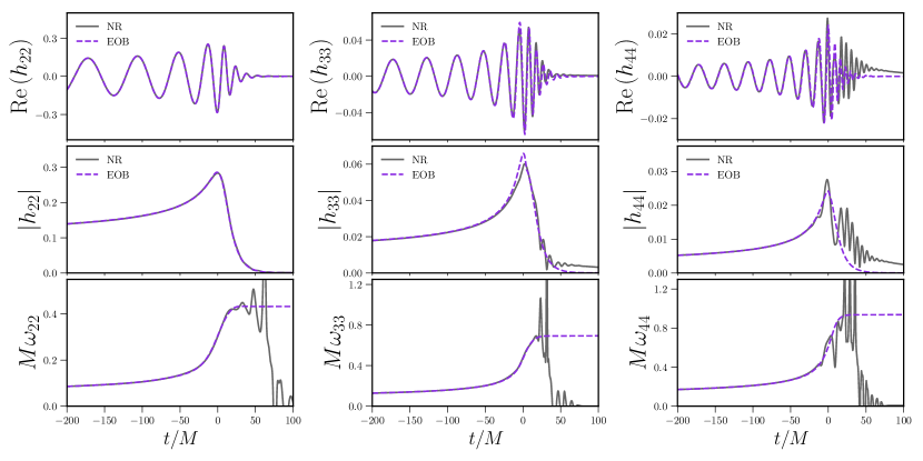
Figure 21: Strain, amplitude and instantaenous frequency for SXS:BBH:0039. Whilst the $(2,2)$ and $(3,3)$ modes are well-behaved, the $(4,4)$ mode demonstrates unphysical features, as seen by the non-monotonic behavior of the amplitude in the merger-ringdown and the strong, oscillatory features in the frequency. This is an example of how NR systematics can lead to relatively poor mismatches against the EOB model.

Appendix C Analytic modeling of the multipolar ringdown waveform

C.1 Introduction

In this Appendix we discuss the fits of the NR data needed for completing TEOBiResumS_SM through merger and ringdown. The fits concern: (i) frequency and amplitude at the peak of each multipole; (ii) the time delays $\Delta t_{\ell m}$ between the peak of each multipole and the peak of the $(2,2)$ mode; (iii) fits for waveforms quantities at the location at the NQC extraction point. Technical details are all listed in Sec. III D and Sec. V A of Ref. Nagar et al. (2019b) and we address the reader there for complementary information. In Sec. C.2 below we report fits of various waveform quantities at the peak of each multipole, that is amplitude, frequency and time-delay $\left(A_{\ell m}^{\rm peak},\omega_{\ell m}^{\rm peak},\Delta t_{\ell m}\right)$. Following Refs. Damour and Nagar (2014b); Del Pozzo and Nagar (2017); Nagar et al. (2018, 2019b), the postpeak waveform needs three additional parameters $\left(c_{3}^{{A}_{\ell m}},c_{3}^{{\phi_{\ell m}}},c_{4}^{{\phi_{\ell m}}}\right)$ to be fitted to NR data. This is discussed in Sec. C.3 below. We present spin-dependent fits for multipoles $(2,2),(3,3),(4,4),(5,5)$, although, for robustness, we prefer to use the nonspinning fits discussed in Nagar et al. (2019b) except for the $(2,2)$ mode. This gives a rather accurate representation of the waveform provided that the other quantities (e.g. the peak ones) incorporate the complete spin dependence. The fits of the quasi-normal-mode frequencies and (inverse) damping timpes entering $\left(\omega_{1}^{\ell m},\alpha_{1}^{\ell m},\alpha_{21}^{\ell m}\right)$ are given in Nagar et al. (2019b). The waveform quantities used to determine the NQC corrections to the waveform amplitude and phase, $\left(A_{\ell m}^{\rm NQC},\omega_{\ell m}^{\rm NQC},\dot{A}_{\ell m}^{\rm NQC},\dot{\omega}_{\ell m}^{\rm NQC}\right)$ are usually obtained analytically from the postpeak template and all details are collected in Sec. C.5 below. For the $(4,4)$ mode, however, this procedure cannot deliver an accurate time-derivative of the waveform amplitude, so that a dedicated fit is given. In the case of the $(\ell,m)=(2,2)$ mode fits for all 4 NQC quanties are also given. Unless otherwise stated all fits are done using fitnlm of matlab and NonLinearModelFit of MATHEMATICA. All fits exclusively use the the calibration set taken from the BAM catalog, test-particle data and the calibration set of SXS waveforms listed in Appendix III. The exception is $\Delta t_{21}$, which is informed additionally by the test set of SXS waveforms.

C.2 Modeling the peak of each multipole

Firs of all, let us recall some symmetric combinations of the spin variables that will be useful later on

$$\hat{S} \equiv\frac{S_{1}+S_{2}}{M^{2}}\ =\frac{1}{2}\left(\tilde{a}_{0}+X_{12}\tilde{a}_{12}\right),$$ (57)

$$\bar{S} \equiv\frac{S_{1}-S_{2}}{M^{2}}\ =\frac{1}{2}\left(X_{12}\tilde{a}_{0}+\tilde{a}_{12}\right).$$ (58)

We refer to the multipolar decomposition of the strain

$$h\equiv h_{+}-ih_{\times}=\sum_{\ell,m}h_{\ell m}{}_{-2}Y_{\ell m}(\iota,\varphi)\ .$$ (59)

Here ${}_{-2}Y_{\ell m}$ are the $s=2$ spin-weighted, spherical harmonics. $\iota$ and $\varphi$ are the polar (with respect to the direction of the orbital angular momentum) and azimuthal angle in the source frame. Each multipole is decomposed in amplitude $A_{\ell m}$ and a phase $\phi_{\ell m}$ as

$$h_{\ell m}=A_{\ell m}e^{{\rm i}\phi_{\ell m}}\ .$$ (60)

The instantaneous GW frequency $\omega_{\ell m}$ is defined as

$$\omega_{\ell m}\equiv-\dot{\phi}_{\ell m},$$ (61)

where the dot indicate the time derivative. Motivated by the leading-order analytical behavior of each multipole, we introduce the following rescaled multipolar amplitudes $\hat{A}_{\ell m}$:

$$\hat{A}_{22} \equiv A_{22}/\left[\nu\left(1-\hat{S}\omega_{22}\right)\right],$$ (62)

$$\hat{A}_{21} \equiv A_{21}/\nu,$$ (63)

$$\hat{A}_{33} \equiv A_{33}/\nu,$$ (64)

$$\hat{A}_{32} \equiv A_{32}/\left[\nu\left(1-\tilde{a}_{0}\left(\omega_{32}/2\right)^{1/3}\right)\right],$$ (65)

$$\hat{A}_{44} \equiv A_{44}/\left[\nu\left(1-\frac{1}{2}\hat{S}\omega_{44}\right)\right],$$ (66)

$$\hat{A}_{43} \equiv A_{43}/\nu,$$ (67)

$$\hat{A}_{42} \equiv A_{42}/\left[\nu\left(1-\tilde{a}_{0}\left(\omega_{42}/2\right)^{1/3}\right)\right].$$ (68)

Then one defines the time where each $(\ell,m)$ mode peaks as

$$t^{\rm peak}_{\ell m}\equiv t\left({\rm max}\left[\hat{A}_{\ell m}\right]\right),$$ (69)

and the merger time, that is defined as the peak of the $(2,2)$ mode, i.e.

$$t^{\rm mrg}\equiv t^{\rm peak}_{22}.$$ (70)

One then defines the time-delay between merger time and the time where each mode peak, as

$$\Delta t_{\ell m}\equiv t^{\rm peak}_{\ell m}-t_{\rm mrg}$$ (71)

For shortness, we denote quantities calculated at a given time using the corresponding superscript, e.g.

$$\hat{A}_{\ell m}^{\rm peak}\equiv\hat{A}_{\ell m}\left(t^{\rm peak}_{\ell m}\right).$$ (72)

Let us now give all details on a mode-by-mode basis.

C.2.1 $(\ell,m)=(2,2)$ multipole

We start by describing the template with which $\omega_{22}^{\rm mrg}$ and $\hat{A}_{22}^{\rm mrg}$ were fitted. The same structure is used both for the amplitude and frequency at merger. We here present it explicitly for $\omega_{22}^{\rm mrg}$, w hile the same for $\hat{A}_{22}^{\rm mrg}$ is obtained by suitably changing the coefficient labels. The frequency at merger $\omega_{22}^{\rm mrg}$ is factorized as

$$\omega_{22}^{\rm mrg}=\omega_{22}^{{\rm mrg}_{0}}\omega_{22}^{\rm orb}(\nu)\omega_{22}^{\hat{S}}(\hat{S},X_{12})\ ,$$ (73)

where $\omega_{22}^{{\rm mrg}_{0}}$ is the value of the merger frequency obtained from a nonspinning test-particle waveform (see e.g. Table 3 of Harms et al. (2014)). The nonspinning $\nu$-dependence is then introduced by fitting the nonspinning data with a template of the form

$$\omega_{22}^{\rm orb}(\nu)=1+a^{\omega}_{1}\nu+a^{\omega}_{2}\nu^{2}\ ,$$ (74)

where the coefficients $a^{\omega}_{i}$ are determined using 19 non-spinning SXS waveforms with mass ratios $1\leq m_{1}/m_{2}\leq 10$. The spin dependence is introduced in two steps: first one accurately fits the spin-dependence of equal-mass data. Then, additional flexibility to incorporate the spinning, unequal-mass data is introduced. More precisely the equal-mass, spin-dependence is obtained with

$$\omega_{22}^{\hat{S}}(\hat{S},X_{12}=0)=\frac{1+b^{\omega_{m_{1}=m_{2}}}_{1}\hat{S}+b^{\omega_{m_{1}=m_{2}}}_{2}\hat{S}^{2}}{1+b^{\omega_{m_{1}=m_{2}}}_{3}\hat{S}},$$ (75)

which is informed by 39 equal-mass, spin-aligned, SXS waveforms. The additional dependence on mass ratio is incorporated substituting into Eq. (75)

$$b^{\omega_{m_{1}=m_{2}}}_{i}\rightarrow\frac{b^{\omega_{m_{1}=m_{2}}}_{i}+c^{\omega}_{i1}X_{12}}{1+c^{\omega}_{i2}X_{12}}\ ,$$ (76)

with $i=\left\{1,3\right\}$. where the additional coefficients $c_{ij}$ are fitted using test-particle data, 77 additional SXS spinning waveforms and 14 additional NR waveforms from BAM. The coefficients are explicitly given in Table 20.

Table 20: Explicit coefficients and their errors for the merger frequency and amplitude fits of the $(2,2)$ mode. The analytic template of the fit is defined in Eqs. (73) – (76).

$\omega_{22}^{{\rm mrg}_{0}}$	$=$	$\;\;\;0.273356$		$\hat{A}_{22}^{{\rm mrg}_{=0}}$	$=$	$\;\;\;1.44959$
$a^{\omega}_{1}$	$=$	$\;\;\;0.84074$	$\pm 0.014341$	$a^{\hat{A}}_{1}$	$=$	$-0.041285$	$\pm 0.0078878$
$a^{\omega}_{2}$	$=$	$\;\;\;1.6976$	$\pm 0.075488$	$a^{\hat{A}}_{2}$	$=$	$\;\;\;1.5971$	$\pm 0.041521$
$b^{\omega_{m_{1}=m_{2}}}_{1}$	$=$	$-0.42311$	$\pm 0.088583$	$b^{\hat{A}_{m_{1}=m_{2}}}_{1}$	$=$	$-0.74124$	$\pm 0.016178$
$b^{\omega_{m_{1}=m_{2}}}_{2}$	$=$	$-0.066699$	$\pm 0.042978$	$b^{\hat{A}_{m_{1}=m_{2}}}_{2}$	$=$	$-0.088705$	$\pm 0.0081611$
$b^{\omega_{m_{1}=m_{2}}}_{3}$	$=$	$-0.83053$	$\pm 0.084516$	$b^{\hat{A}_{m_{1}=m_{2}}}_{3}$	$=$	$-1.0939$	$\pm 0.015318$
$c^{\omega}_{11}$	$=$	$\;\;\;0.15873$	$\pm 0.1103$	$c^{\hat{A}}_{11}$	$=$	$\;\;\;0.44467$	$\pm 0.037352$
$c^{\omega}_{12}$	$=$	$-0.43361$	$\pm 0.2393$	$c^{\hat{A}}_{12}$	$=$	$-0.32543$	$\pm 0.081211$
$c^{\omega}_{21}$	$=$	$\;\;\;0.60589$	$\pm 0.076215$	$c^{\hat{A}}_{31}$	$=$	$\;\;\;0.45828$	$\pm 0.066062$
$c^{\omega}_{22}$	$=$	$-0.71383$	$\pm 0.096828$	$c^{\hat{A}}_{32}$	$=$	$-0.21245$	$\pm 0.080254$

C.2.2 $(\ell,m)=(2,1)$ multipole

The procedure followed for the subdominant modes is similar to what is done for the $(2,2)$. There are however some differences. First of all, the peak time shift $\Delta t_{\ell m}$ is also fitted to NR simulations. Second, basing ourselves to the analytical behavior of the multipolar waveform, we have decided to use different factorizations and different variables to model each mode. For example, the $(2,1)$ multipole (and every $m$-odd mode) vanishes because of symmetry in the equal-mass equal-spin case. This has brought us to consider the following factorization for $\hat{A}_{21}^{\rm peak}$, which is written as

$$\hat{A}_{21}^{\rm peak}=\hat{A}_{21}^{{\rm peak}_{0}}X_{12}\hat{A}_{21}^{\rm orb}\left(\nu\right)+\hat{A}_{21}^{\rm Spin}\left(\bar{S},\nu\right).$$ (77)

where $\hat{A}_{21}^{{\rm peak}_{0}}$ is the peak amplitude in the test-particle limit. The factor $\hat{A}_{21}^{\rm orb}$ is informed by non-spinning waveforms and is fitted with the template

$$\hat{A}_{21}^{\rm orb}(\nu)=\frac{1+a^{\hat{A}_{21}}_{1}\nu+a^{\hat{A}_{21}}_{2}\nu^{2}}{1+a^{\hat{A}_{21}}_{3}\nu}\ .$$ (78)

The spin dependence is first captured in the test-particle limit with the function

$$\hat{A}_{21}^{\rm Spin}(\bar{S},\nu=0)=\frac{1+b^{\hat{A}^{0}_{21}}_{1}\bar{S}+b^{\hat{A}^{0}_{21}}_{2}\bar{S}^{2}}{1+b^{\hat{A}^{0}_{21}}_{3}\bar{S}}\ .$$ (79)

The $\nu$-dependence is then modeled via the replacement

$$b^{\hat{A}^{0}_{21}}_{i}\rightarrow b^{\hat{A}^{0}_{21}}_{i}+c^{\hat{A}_{21}}_{i1}\nu+c^{\hat{A}_{21}}_{i2}\nu^{2}\ ,$$ (80)

with $i=\left\{1,2,3\right\}$.

The gravitational wave frequency $\omega_{21}$ is instead factorized as

$$\omega^{\rm peak}_{21}=\omega^{{\rm peak}_{0}}_{21}\omega^{\rm orb}_{21}(\nu)\omega^{\rm Spin}_{21}\left(\hat{S},\nu\right),$$ (81)

where the $\nu$-dependence of the nonspinning part is modeled as

$$\omega^{\rm orb}_{21}(\nu)=1+a^{\omega_{21}}_{1}\nu+a^{\omega_{21}}_{2}\nu^{2}\ .$$ (82)

The spin dependence is fitted first in the test-particle limit

$$\omega^{\rm Spin}_{21}\left(\hat{S},\nu=0\right)=1+b^{\omega^{0}_{21}}_{1}\hat{S}+b^{\omega^{0}_{21}}_{2}\hat{S}^{2}\ ,$$ (83)

and then extended to a general mass ratio via the replacement

$$b^{\omega^{0}_{21}}_{i}\rightarrow b^{\omega^{0}_{21}}_{i}+c^{\omega_{21}}_{i}\nu\ ,$$ (84)

with $i=\left\{1,2\right\}$.

Finally, to represent analytically the time-delay $\Delta t_{21}$ we use

$$\Delta t_{21}=\Delta t_{21}^{\rm orb}(\nu)\Delta t_{21}^{\rm spin}\left(\bar{S},X_{12}\right)\ ,$$ (85)

where the orbital behavior is factorized into two separate parts before fitting with

$$\Delta t_{21}^{\rm orb}(\nu)= \left(\Delta t_{21}^{0}(1-4\nu)+\Delta t_{21}^{\nu=1/4}4\nu\right)$$ (86)

$$\;\;\;\times\left(1+a_{1}^{\Delta t_{21}}\nu\sqrt{1-4\nu}\right)\ .$$

The factor $\Delta t_{21}^{\nu=1/4}$ is obtained by fitting a 2nd-order polynomial, in $\hat{a}_{0}$ to the equal-mass waveforms. $\Delta t_{21}^{0}$ is the test-particle value. The equal-mass spin behavior is fitted with

$$\Delta t_{21}^{\rm spin}\left(\bar{S},X_{12}=0\right)=1+b_{1}^{\Delta t_{21}^{\nu=1/4}}\hat{a}_{0}+b_{2}^{\Delta t_{21}^{\nu=1/4}}\hat{a}_{0}^{2}\ ,$$ (87)

while the comparable mass case is extrapolated using

$$b_{1}^{\Delta t_{21}^{\nu=1/4}}\rightarrow\frac{b_{1}^{\Delta t_{21}^{0}}+c_{i1}^{\Delta t_{21}}X_{12}}{1+c_{i2}^{\Delta t_{21}}X_{12}}\ ,$$ (88)

with $i=\left\{1,2\right\}$. The outcome of the fit, with the explicit values of all coefficients, id found in Table 21.

Table 21: Explicit coefficients of the fits of $\hat{A}_{21}^{\rm peak}$, $\omega_{21}^{\rm peak}$ and $\Delta t_{21}$.

$\hat{A}_{21}^{{\rm peak}_{0}}$	$=$	$0.523878$	$\omega_{21}^{{\rm peak}_{0}}$	$=$	$0.290643$	$\Delta t_{21}^{0}$	$=$	$11.75925$
$a^{\hat{A}_{21}}_{1}$	$=$	$3.33622$	$a^{\omega_{21}}_{1}$	$=$	$-0.563075$	$\Delta t_{21}^{\nu=1/4}$	$=$	$6.6264$
$a^{\hat{A}_{21}}_{2}$	$=$	$3.47085$	$a^{\omega_{21}}_{2}$	$=$	$3.28677$	$a^{\Delta t_{21}}_{1}$	$=$	$-2.0728$
$a^{\hat{A}_{21}}_{3}$	$=$	$4.76236$
$b^{\hat{A}_{21}^{0}}_{1}$	$=$	$-0.428186$	$b^{\omega_{21}^{0}}_{1}$	$=$	$0.179639$	$b^{\Delta t_{21}^{0}}_{1}$	$=$	$0.0472289$
$b^{\hat{A}_{21}^{0}}_{2}$	$=$	$-0.335659$	$b^{\omega_{21}^{0}}_{2}$	$=$	$-0.302122$	$b^{\Delta t_{21}^{0}}_{2}$	$=$	$0.115583$
$b^{\hat{A}_{21}^{0}}_{3}$	$=$	$0.828923$
$c^{\hat{A}_{21}}_{11}$	$=$	$0.891139$	$c^{\omega_{21}}_{1}$	$=$	$-1.20684$	$c^{\Delta t_{21}}_{11}$	$=$	$-1976.13$
$c^{\hat{A}_{21}}_{12}$	$=$	$-5.191702$	$c^{\omega_{21}}_{2}$	$=$	$0.425645$	$c^{\Delta t_{21}}_{12}$	$=$	$3719.88$
$c^{\hat{A}_{21}}_{21}$	$=$	$3.480139$				$c^{\Delta t_{21}}_{21}$	$=$	$-2545.41$
$c^{\hat{A}_{21}}_{22}$	$=$	$10.237782$				$c^{\Delta t_{21}}_{22}$	$=$	$5277.62$
$c^{\hat{A}_{21}}_{31}$	$=$	$-13.867475$
$c^{\hat{A}_{21}}_{32}$	$=$	$10.525510$

C.2.3 $(\ell,m)=(3,3)$ multipole

For this mode, the peak amplitude is written as the sum of two terms

$$\hat{A}_{33}^{\rm peak}=\hat{A}_{33}^{{\rm peak}_{0}}X_{12}\hat{A}_{33}^{\rm orb}(\nu)+\hat{A}_{33}^{\rm Spin}(\tilde{a}_{12},\nu)\ ,$$ (89)

where $\hat{A}_{33}^{{\rm peak}_{0}}$ is the peak amplitude in the test particle limit. The orbital term is modeled as

$$\hat{A}_{33}^{\rm orb}(\nu)=\frac{1+a^{\hat{A}_{33}}_{1}\nu+a^{\hat{A}_{33}}_{2}\nu^{2}}{1+a^{\hat{A}_{33}}_{3}\nu}\ .$$ (90)

The spin dependence is first fitted in the test-particle limit using

$$\hat{A}_{33}^{\rm Spin}(\tilde{a}_{12},\nu=0)=\frac{b^{\hat{A}^{0}_{33}}_{1}\tilde{a}_{12}}{1+b^{\hat{A}^{0}_{33}}_{2}\tilde{a}_{12}}\ ,$$ (91)

and then extended to comparable masses via the replacements

$$b^{\hat{A}^{0}_{33}}_{1} \rightarrow \frac{b^{\hat{A}^{0}_{33}}_{1}+c^{\hat{A}_{33}}_{11}\nu}{1+c^{\hat{A}_{33}}_{12}\nu+c^{\hat{A}_{33}}_{13}\nu^{2}}\ ,$$ (92)

$$b^{\hat{A}^{0}_{33}}_{2} \rightarrow \frac{b^{\hat{A}^{0}_{33}}_{2}+c^{\hat{A}_{33}}_{21}\nu}{1+c^{\hat{A}_{33}}_{22}\nu+c^{\hat{A}_{33}}_{23}\nu^{2}}\ .$$ (93)

The istantaneous frequency $\omega_{33}$ is factorized as

$$\omega^{\rm peak}_{33}=\omega^{{\rm peak}_{0}}_{33}\omega^{\rm orb}_{33}(\nu)\omega^{\rm Spin}_{33}\left(\hat{S},\nu\right)\ ,$$ (94)

where

$$\omega^{\rm orb}_{33}(\nu)=1+a^{\omega_{33}}_{1}\nu+a^{\omega_{33}}_{2}\nu^{2}\ .$$ (95)

The test-particle spin factor is given by

$$\omega^{\rm Spin}_{33}\left(\hat{S},\nu=0\right)=\frac{1+b^{\omega^{0}_{33}}_{1}\hat{S}+b^{\omega^{0}_{33}}_{2}\hat{S}^{2}}{1+b^{\omega^{0}_{33}}_{3}\hat{S}}\ ,$$ (96)

while the general spin-dependence stems from the replacement

$$b^{\omega^{0}_{33}}_{i}\rightarrow\frac{b^{\omega^{0}_{33}}_{i}+c^{\omega_{33}}_{i1}\nu}{1+c^{\omega_{33}}_{i2}\nu}\ ,$$ (97)

with $i=\left\{1,3\right\}$.

To describe $\Delta t_{33}$ we start from the expression

$$\Delta t_{33}=\Delta t_{33}^{0}\Delta t_{33}^{\rm orb}(\nu)\Delta t_{33}^{\rm spin}\left(\hat{S},\nu\right)\ ,$$ (98)

with

$$\Delta t_{33}^{\rm orb}(\nu) =1+a_{1}^{\Delta t_{33}}\nu+a_{2}^{\Delta t_{33}}\nu^{2}\ ,$$ (99)

$$\Delta t_{33}^{\rm spin}\left(\hat{S},\nu=0\right) =\frac{1+b_{1}^{\Delta t_{33}^{0}}\hat{S}+b_{2}^{\Delta t_{33}^{0}}\hat{S}^{2}}{1+b_{3}^{\Delta t_{33}^{0}}\hat{S}}\ .$$ (100)

The spin-dependence is obtained from the replacement

$$b_{1}^{\Delta t_{33}^{0}}\rightarrow\frac{b_{1}^{\Delta t_{33}^{0}}+c_{i1}^{\Delta t_{33}}\nu}{1+c_{i2}^{\Delta t_{33}}\nu}\ ,$$ (101)

with $i=\left\{1,2,3\right\}$. The explicit values of the fit coefficients are listed in Table 22.

Table 22: Explicit coefficients of the fits of $\hat{A}_{33}^{\rm peak}$, $\omega_{33}^{\rm peak}$ and $\Delta t_{33}$.

$\hat{A}_{33}^{{\rm peak}_{0}}$	$=$	$0.566017$	$\omega_{33}^{{\rm peak}_{0}}$	$=$	$0.454128$	$\Delta t_{33}^{0}$	$=$	$3.42593$
$a^{\hat{A}_{33}}_{1}$	$=$	$-0.22523$	$a^{\omega_{33}}_{1}$	$=$	$1.08224$	$a^{\Delta t_{33}}_{1}$	$=$	$0.183349$
$a^{\hat{A}_{33}}_{2}$	$=$	$3.0569$	$a^{\omega_{33}}_{2}$	$=$	$2.59333$	$a^{\Delta t_{33}}_{2}$	$=$	$4.22361$
$a^{\hat{A}_{33}}_{3}$	$=$	$-0.396851$
$b^{\hat{A}^{0}_{33}}_{1}$	$=$	$0.100069$	$b^{\omega^{0}_{33}}_{1}$	$=$	$-0.406161$	$b^{\Delta t_{33}^{0}}_{1}$	$=$	$-0.49791$
$b^{\hat{A}^{0}_{33}}_{2}$	$=$	$-0.455859$	$b^{\omega^{0}_{33}}_{2}$	$=$	$-0.0647944$	$b^{\Delta t_{33}^{0}}_{2}$	$=$	$-0.18754$
			$b^{\omega^{0}_{33}}_{3}$	$=$	$-0.748126$	$b^{\Delta t_{33}^{0}}_{3}$	$=$	$-1.07291$
$c^{\hat{A}_{33}}_{11}$	$=$	$-0.401156$	$c^{\omega_{33}}_{11}$	$=$	$0.85777$	$c^{\Delta t_{33}}_{11}$	$=$	$-1.9478$
$c^{\hat{A}_{33}}_{12}$	$=$	$-0.141551$	$c^{\omega_{33}}_{12}$	$=$	$-0.70066$	$c^{\Delta t_{33}}_{12}$	$=$	$13.9828$
$c^{\hat{A}_{33}}_{13}$	$=$	$-15.4949$	$c^{\omega_{33}}_{31}$	$=$	$2.97025$	$c^{\Delta t_{33}}_{21}$	$=$	$1.25084$
$c^{\hat{A}_{33}}_{21}$	$=$	$1.84962$	$c^{\omega_{33}}_{32}$	$=$	$-3.96242$	$c^{\Delta t_{33}}_{22}$	$=$	$-3.41811$
$c^{\hat{A}_{33}}_{22}$	$=$	$-2.03512$				$c^{\Delta t_{33}}_{31}$	$=$	$-1043.15$
$c^{\hat{A}_{33}}_{23}$	$=$	$-4.92334$				$c^{\Delta t_{33}}_{32}$	$=$	$1033.85$

C.2.4 $(\ell,m)=(3,2)$ multipole

The peak amplitude of the $(3,2)$ mode is fitted with a factorized template of the form

$$\hat{A}_{32}^{\rm peak}=\hat{A}_{32}^{{\rm peak}_{0}}\left(1-3\nu\right)\hat{A}_{32}^{\rm orb}\left(\nu\right)\hat{A}_{32}^{\rm Spin}\left(\bar{S},\nu\right)\ ,$$ (102)

where $\hat{A}_{32}^{{\rm peak}_{0}}$ is the peak amplitude of the mode in the test-particle limit. The factor $\hat{A}_{32}^{\rm orb}$ is informed by non-spinning waveforms and is fitted with the template

$$\hat{A}_{32}^{\rm orb}(\nu)=\frac{1+a^{\hat{A}_{32}}_{1}\nu+a^{\hat{A}_{32}}_{2}\nu^{2}}{1+a^{\hat{A}_{32}}_{3}\nu}\ .$$ (103)

The spin dependence is first captured for the test-particle limit with the function

$$\hat{A}_{32}^{\rm Spin}(\bar{S},\nu=0)=\frac{1+b^{\hat{A}^{0}_{32}}_{1}\tilde{a}_{0}}{1+b^{\hat{A}^{0}_{32}}_{2}\tilde{a}_{0}}\ ,$$ (104)

while the $\nu$-dependence enters via the replacement

$$b^{\hat{A}^{0}_{32}}_{i}\rightarrow\frac{b^{\hat{A}^{0}_{32}}_{i}+c^{\hat{A}_{32}}_{i1}\nu+c^{\hat{A}_{32}}_{i2}\nu^{2}}{1+c^{\hat{A}_{32}}_{i3}\nu+c^{\hat{A}_{32}}_{i4}\nu^{2}}\ ,$$ (105)

with $i=\left\{1,2\right\}$.

The instantaneous frequency $\omega_{32}$ mode is factorized as

$$\omega^{\rm peak}_{32}=\omega^{{\rm peak}_{0}}_{32}\omega^{\rm orb}_{32}(\nu)\omega^{\rm Spin}_{32}\left(\tilde{a}_{0},\nu\right)\ .$$ (106)

The orbital dependence is modeled as

$$\omega^{\rm orb}_{32}(\nu)=\frac{1+a^{\omega_{32}}_{1}\nu+a^{\omega_{32}}_{2}\nu^{2}}{1+a^{\omega_{32}}_{3}\nu+a^{\omega_{32}}_{4}\nu^{2}}\ .$$ (107)

The spin dependence is fitted first for the equal-mass case

$$\omega^{\rm Spin}_{32}\left(\tilde{a}_{0},\nu=1/4\right)=\frac{1+b^{\omega^{\nu=1/4}_{32}}_{1}\tilde{a}_{0}+b^{\omega^{\nu=1/4}_{32}}_{2}\tilde{a}_{0}^{2}}{1+b^{\omega^{\nu=1/4}_{32}}_{3}\tilde{a}_{0}}\ ,$$ (108)

while the additional dependence on the mass ratio enters via the replacements

$$b^{\omega^{0}_{32}}_{i}\rightarrow\frac{b^{\omega^{\nu=1/4}_{32}}_{i}+c^{\omega_{32}}_{i1}X_{12}+c^{\omega_{32}}_{i2}X^{2}_{12}}{1+c^{\omega_{32}}_{i3}X_{12}}\ ,$$ (109)

with $i=\left\{1,2\right\}$. The coefficients of $\hat{A}^{\rm peak}_{32}$ and $\omega^{\rm peak}_{32}$ are explicitly listed in Table 27.

Moving to $\Delta t_{32}$, it is given by

$$\Delta t_{32}=\Delta t_{32}^{0}\Delta t_{32}^{\rm orb}(\nu)\Delta t_{32}^{\rm spin}\left(\hat{S},\nu\right)\ ,$$ (110)

where the orbital behavior is fitted with

$$\Delta t_{32}^{\rm orb}(\nu)=\frac{1+a^{\Delta t_{32}}_{1}\nu+a^{\Delta t_{32}}_{2}\nu^{2}}{1+a^{\Delta t_{32}}_{3}\nu+a^{\Delta t_{32}}_{4}\nu^{2}}\ .$$ (111)

The spin behavior is more complicated than the corresponding term of other modes. This is separated into two sectors, as

$$\Delta t_{32}^{\rm spin}\left(\hat{S},\nu\right)=~{} \Delta t_{32}^{{\rm spin}_{\nu>1/5}}\left(\hat{S},\nu\right)\Theta\left(\nu-1/5\right)$$

$$+\Delta t_{32}^{{\rm spin}_{\nu\leq 1/5}}\left(\hat{S},\nu\right)\left[1-\Theta\left(\nu-1/5\right)\right]\ ,$$ (112)

where $\Theta$ denotes the Heaviside step function. In the $\nu>1/5$ regime the fit is first done to the equal-mass case

$$\Delta t_{32}^{{\rm spin}_{\nu>1/5}}\left(\hat{S},\nu=1/4\right)=\frac{1+b^{\Delta t_{32}^{\nu=1/4}}_{1}\hat{S}+b^{\Delta t_{32}^{\nu=1/4}}_{2}\hat{S}^{2}}{1+b^{\Delta t_{32}^{\nu=1/4}}_{3}\hat{S}}\ .$$ (113)

Then it is extrapolated following

$$b^{\Delta t_{32}^{\nu=1/4}}_{i}\rightarrow\frac{b^{\Delta t_{32}^{\nu=1/4}}_{1}+c^{\Delta t_{32}}_{i1}X_{12}+c^{\Delta t_{32}}_{i2}X_{12}^{2}+c^{\Delta t_{32}}_{i3}X_{12}^{3}}{1+c^{\Delta t_{43}}_{i4}X_{12}+c^{\Delta t_{43}}_{i5}X_{12}^{2}}\ ,$$ (114)

with $i=\left\{1,2,3\right\}$.

In the $\nu\leq 1/5$ regime the fit is first done to the equal-mass case

$$\Delta t_{32}^{{\rm spin}_{\nu\leq 1/5}}\left(\hat{S},\nu=0\right)=\frac{1+b^{\Delta t_{32}^{0}}_{1}\hat{S}+b^{\Delta t_{32}^{0}}_{2}\hat{S}^{2}}{1+b^{\Delta t_{32}^{0}}_{3}\hat{S}}\ .$$ (115)

Then it is extrapolated following

$$b^{\Delta t_{32}^{0}}_{i}\rightarrow\frac{b^{\Delta t_{32}^{0}}_{1}+c^{\Delta t_{32}}_{i1}\nu+c^{\Delta t_{32}}_{i2}\nu^{2}+c^{\Delta t_{32}}_{i3}\nu^{3}}{1+c^{\Delta t_{32}}_{i4}\nu+c^{\Delta t_{32}}_{i5}\nu^{2}}\ ,$$ (116)

with $i=\left\{1,2,3\right\}$. The coefficients appearing in $\Delta t_{32}$ are shown in Table 24.

Table 23: Explicit coefficients of the fits of $\hat{A}_{32}^{\rm peak}$ and $\omega_{32}^{\rm peak}$.

$\hat{A}_{32}^{{\rm peak}_{0}}$	$=$	$0.199019$	$\omega_{32}^{{\rm peak}_{0}}$	$=$	$0.451607$
$a^{\hat{A}_{32}}_{1}$	$=$	$-6.06831$	$a^{\omega_{32}}_{1}$	$=$	$-9.13525$
$a^{\hat{A}_{32}}_{2}$	$=$	$10.7505$	$a^{\omega_{32}}_{2}$	$=$	$21.488$
$a^{\hat{A}_{32}}_{3}$	$=$	$-3.68883$	$a^{\omega_{32}}_{3}$	$=$	$-8.81384$
			$a^{\omega_{32}}_{4}$	$=$	$20.0595$
$b^{\hat{A}_{32}^{0}}_{1}$	$=$	$-0.258378$	$b^{\omega_{32}^{\nu=1/4}}_{1}$	$=$	$-0.458126$
$b^{\hat{A}_{32}^{0}}_{2}$	$=$	$0.679163$	$b^{\omega_{32}^{\nu=1/4}}_{2}$	$=$	$0.0474616$
			$b^{\omega_{32}^{\nu=1/4}}_{3}$	$=$	$-0.486049$
$c^{\hat{A}_{32}}_{11}$	$=$	$4.36263$	$c^{\omega_{32}}_{11}$	$=$	$3.25319$
$c^{\hat{A}_{32}}_{12}$	$=$	$-12.5897$	$c^{\omega_{32}}_{12}$	$=$	$0.535555$
$c^{\hat{A}_{32}}_{13}$	$=$	$-7.73233$	$c^{\omega_{32}}_{13}$	$=$	$-8.07905$
$c^{\hat{A}_{32}}_{14}$	$=$	$16.2082$	$c^{\omega_{32}}_{21}$	$=$	$1.00066$
$c^{\hat{A}_{32}}_{21}$	$=$	$3.04724$	$c^{\omega_{32}}_{22}$	$=$	$-1.1333$
$c^{\hat{A}_{32}}_{22}$	$=$	$46.5711$	$c^{\omega_{32}}_{23}$	$=$	$0.601572$
$c^{\hat{A}_{32}}_{23}$	$=$	$2.10475$
$c^{\hat{A}_{32}}_{24}$	$=$	$56.9136$

Table 24: Explicit coefficients of $\Delta t_{32}$.

$\Delta t_{32}^{0}$	$=$	$9.16665$	$c^{\Delta t_{32}^{\nu}}_{11}$	$=$	$-0.037634$	$c^{\Delta t_{32}^{X_{12}}}_{11}$	$=$	$2.497188$
$a^{\Delta t_{32}}_{1}$	$=$	$-11.3497$	$c^{\Delta t_{32}^{\nu}}_{12}$	$=$	$12.456704$	$c^{\Delta t_{32}^{X_{12}}}_{12}$	$=$	$-7.532596$
$a^{\Delta t_{32}}_{2}$	$=$	$32.9144$	$c^{\Delta t_{32}^{\nu}}_{13}$	$=$	$2.670868$	$c^{\Delta t_{32}^{X_{12}}}_{13}$	$=$	$4.645986$
$a^{\Delta t_{32}}_{3}$	$=$	$-8.36579$	$c^{\Delta t_{32}^{\nu}}_{14}$	$=$	$-12.255859$	$c^{\Delta t_{32}^{X_{12}}}_{14}$	$=$	$-3.652524$
$a^{\Delta t_{32}}_{4}$	$=$	$20.1017$	$c^{\Delta t_{32}^{\nu}}_{15}$	$=$	$37.843505$	$c^{\Delta t_{32}^{X_{12}}}_{15}$	$=$	$3.398687$
$b^{\Delta t_{32}^{0}}_{1}$	$=$	$-0.34161$	$c^{\Delta t_{32}^{\nu}}_{21}$	$=$	$-25.058475$	$c^{\Delta t_{32}^{X_{12}}}_{21}$	$=$	$7.054185$
$b^{\Delta t_{32}^{0}}_{2}$	$=$	$-0.46107$	$c^{\Delta t_{32}^{\nu}}_{22}$	$=$	$449.470722$	$c^{\Delta t_{32}^{X_{12}}}_{22}$	$=$	$-12.260185$
$b^{\Delta t_{32}^{0}}_{3}$	$=$	$0.34744$	$c^{\Delta t_{32}^{\nu}}_{23}$	$=$	$-1413.508735$	$c^{\Delta t_{32}^{X_{12}}}_{23}$	$=$	$5.724802$
$b^{\Delta t_{32}^{\nu=1/4}}_{1}$	$=$	$0.15477$	$c^{\Delta t_{32}^{\nu}}_{24}$	$=$	$-11.852596$	$c^{\Delta t_{32}^{X_{12}}}_{24}$	$=$	$-3.242611$
$b^{\Delta t_{32}^{\nu=1/4}}_{2}$	$=$	$-0.755639$	$c^{\Delta t_{32}^{\nu}}_{25}$	$=$	$41.348059$	$c^{\Delta t_{32}^{X_{12}}}_{25}$	$=$	$2.714232$
$b^{\Delta t_{32}^{\nu=1/4}}_{3}$	$=$	$0.21816$	$c^{\Delta t_{32}^{\nu}}_{31}$	$=$	$-5.650710$	$c^{\Delta t_{32}^{X_{12}}}_{31}$	$=$	$2.614565$
			$c^{\Delta t_{32}^{\nu}}_{32}$	$=$	$-9.567484$	$c^{\Delta t_{32}^{X_{12}}}_{32}$	$=$	$-9.507583$
			$c^{\Delta t_{32}^{\nu}}_{33}$	$=$	$173.182999$	$c^{\Delta t_{32}^{X_{12}}}_{33}$	$=$	$7.321586$
			$c^{\Delta t_{32}^{\nu}}_{34}$	$=$	$-10.938605$	$c^{\Delta t_{32}^{X_{12}}}_{34}$	$=$	$-3.937568$
			$c^{\Delta t_{32}^{\nu}}_{35}$	$=$	$35.670656$	$c^{\Delta t_{32}^{X_{12}}}_{35}$	$=$	$4.584970$

C.2.5 $(\ell,m)=(4,4)$ multipole

The peak amplitude of the $(4,4)$ mode is fitted with

$$\hat{A}_{44}^{\rm peak}=\hat{A}_{44}^{{\rm peak}_{0}}\left(1-3\nu\right)\hat{A}_{44}^{\rm orb}\left(\nu\right)\hat{A}_{44}^{\rm Spin}\left(\hat{S},\nu\right)\ ,$$ (117)

where $\hat{A}_{44}^{{\rm peak}_{0}}$ is the peak amplitude of the mode in the test-particle limit. The factor $\hat{A}_{44}^{\rm orb}$ is informed by non-spinning waveforms and is fitted with the template

$$\hat{A}_{44}^{\rm orb}(\nu)=\frac{1+a^{\hat{A}_{44}}_{1}\nu+a^{\hat{A}_{44}}_{2}\nu^{2}}{1+a^{\hat{A}_{44}}_{3}\nu}\ .$$ (118)

The spin dependence is first captured for the test-particle limit with the function

$$\hat{A}_{44}^{\rm Spin}(\hat{S},\nu=0)=\frac{1+b^{\hat{A}^{0}_{44}}_{1}\hat{S}+b^{\hat{A}^{0}_{44}}_{2}\hat{S}^{2}}{1+b^{\hat{A}^{0}_{44}}_{3}\hat{S}}\ ,$$ (119)

and then extended in the comparable mass region of the parameter space through

$$b^{\hat{A}^{0}_{44}}_{i}\rightarrow\frac{b^{\hat{A}^{0}_{44}}_{i}+c^{\hat{A}_{44}}_{i1}\nu+c^{\hat{A}_{44}}_{i2}\nu^{2}}{1+c^{\hat{A}_{44}}_{i3}\nu+c^{\hat{A}_{44}}_{i4}\nu^{2}}\ ,\ {\rm with}\ i=\left\{1,2,3\right\}.$$ (120)

The peak frequency $\omega_{44}$ is factorized as

$$\omega^{\rm peak}_{44}=\omega^{{\rm peak}_{0}}_{44}\omega^{\rm orb}_{44}(\nu)\omega^{\rm Spin}_{44}\left(\hat{S},\nu\right)\ .$$ (121)

The orbital dependence is modeled through

$$\omega^{\rm orb}_{44}(\nu)=\frac{1+a^{\omega_{44}}_{1}\nu+a^{\omega_{44}}_{2}\nu^{2}}{1+a^{\omega_{44}}_{3}\nu+a^{\omega_{44}}_{4}\nu^{2}}\ .$$ (122)

The spin dependence is fitted first for the test-particle limit as

$$\omega^{\rm Spin}_{44}\left(\hat{S},\nu=0\right)=\frac{1+b^{\omega^{0}_{44}}_{1}\hat{S}+b^{\omega^{0}_{44}}_{2}\hat{S}^{2}+b^{\omega^{0}_{44}}_{3}\hat{S}^{3}}{1+b^{\omega^{0}_{33}}_{4}\hat{S}}\ .$$ (123)

The spin dependence in the comparable mass region of the parameter space is modeled through

$$b^{\omega^{0}_{44}}_{i}\rightarrow\frac{b^{\omega^{0}_{44}}_{i}+c^{\omega_{44}}_{i1}\nu+c^{\omega_{44}}_{i2}\nu^{2}}{1+c^{\omega_{44}}_{i3}\nu+c^{\omega_{44}}_{i4}\nu^{2}}\ ,$$ (124)

with $i=\left\{1,2,3,4\right\}$.

We fit $\Delta t_{44}$ in a factorized form as

$$\Delta t_{44}=\Delta t_{44}^{0}\Delta t_{44}^{\rm orb}(\nu)\Delta t_{44}^{\rm spin}\left(\hat{S},X_{12}\right)\ .$$ (125)

The orbital behavior is fitted with

$$\Delta t_{44}^{\rm orb}(\nu)=\frac{1+a_{1}^{\Delta t_{44}}\nu+a_{2}^{\Delta t_{44}}\nu^{2}}{1+a_{3}^{\Delta t_{44}}\nu+a_{4}^{\Delta t_{44}}\nu^{2}}\ ,$$ (126)

while the spinning one is first fitted to equal mass simulations as

$$\Delta t_{44}^{\rm spin}\left(\hat{S},X_{12}=0\right)=\frac{1+b_{1}^{\Delta t_{44}^{\nu=1/4}}\hat{S}}{1+b_{2}^{\Delta t_{44}^{\nu=1/4}}\hat{S}}\ .$$ (127)

The general $\nu$-dependence enters via the replacement

$$b_{i}^{\Delta t_{44}^{\nu=1/4}}\rightarrow b_{i}^{\Delta t_{44}^{\nu=1/4}}+c_{i1}^{\Delta t_{44}}X_{12}+c_{i2}^{\Delta t_{44}}X_{12}^{2}\ ,$$ (128)

with $i=\left\{1,2\right\}$. The explicit values of the fit coefficients can be found in Table 25.

Table 25: Explicit coefficients of the fits of $\hat{A}_{44}^{\rm peak}$, $\omega_{44}^{\rm peak}$ and $\Delta t_{44}$.

$\hat{A}_{44}^{{\rm peak}_{0}}$	$=$	$0.276618$	$\omega_{44}^{{\rm peak}_{0}}$	$=$	$0.635659$	$\Delta t_{44}^{0}$	$=$	$5.27778$
$a^{\hat{A}_{44}}_{1}$	$=$	$-3.7082$	$a^{\omega_{44}}_{1}$	$=$	$-0.964614$	$a^{\Delta t_{44}}_{1}$	$=$	$-8.35574$
$a^{\hat{A}_{44}}_{2}$	$=$	$0.280906$	$a^{\omega_{44}}_{2}$	$=$	$-11.1828$	$a^{\Delta t_{44}}_{2}$	$=$	$17.5288$
$a^{\hat{A}_{44}}_{3}$	$=$	$-3.71276$	$a^{\omega_{44}}_{3}$	$=$	$-2.08471$	$a^{\Delta t_{44}}_{3}$	$=$	$-6.50259$
			$a^{\omega_{44}}_{4}$	$=$	$-6.89287$	$a^{\Delta t_{44}}_{4}$	$=$	$10.1575$
$b^{\hat{A}^{0}_{44}}_{1}$	$=$	$-0.316647$	$b^{\omega^{0}_{44}}_{1}$	$=$	$-0.445192$	$b^{\Delta t_{44}^{\nu=1/4}}_{1}$	$=$	$0.00159701$
$b^{\hat{A}^{0}_{44}}_{2}$	$=$	$-0.062423$	$b^{\omega^{0}_{44}}_{2}$	$=$	$-0.0985658$	$b^{\Delta t_{44}^{\nu=1/4}}_{2}$	$=$	$-1.14134$
$b^{\hat{A}^{0}_{44}}_{3}$	$=$	$-0.852876$	$b^{\omega^{0}_{44}}_{3}$	$=$	$-0.0307812$
			$b^{\omega^{0}_{44}}_{4}$	$=$	$-0.801552$
$c^{\hat{A}_{44}}_{11}$	$=$	$1.2436$	$c^{\omega_{44}}_{11}$	$=$	$-0.92902$	$c^{\Delta t_{4}}_{11}$	$=$	$-2.28656$
$c^{\hat{A}_{44}}_{12}$	$=$	$-1.60555$	$c^{\omega_{44}}_{12}$	$=$	$10.86310$	$c^{\Delta t_{44}}_{12}$	$=$	$1.66532$
$c^{\hat{A}_{44}}_{13}$	$=$	$-4.05685$	$c^{\omega_{44}}_{13}$	$=$	$-4.44930$	$c^{\Delta t_{44}}_{21}$	$=$	$-0.589331$
$c^{\hat{A}_{44}}_{14}$	$=$	$1.59143$	$c^{\omega_{44}}_{14}$	$=$	$3.01808$	$c^{\Delta t_{44}}_{22}$	$=$	$0.708784$
$c^{\hat{A}_{44}}_{21}$	$=$	$0.837418$	$c^{\omega_{44}}_{22}$	$=$	$1.62523$
$c^{\hat{A}_{44}}_{22}$	$=$	$-2.93528$	$c^{\omega_{44}}_{23}$	$=$	$-7.70486$
$c^{\hat{A}_{44}}_{23}$	$=$	$-11.5591$	$c^{\omega_{44}}_{23}$	$=$	$15.06517$
$c^{\hat{A}_{44}}_{24}$	$=$	$34.1863$	$c^{\omega_{44}}_{41}$	$=$	$0.93790$
$c^{\hat{A}_{44}}_{31}$	$=$	$0.950035$	$c^{\omega_{44}}_{42}$	$=$	$8.36038$
$c^{\hat{A}_{44}}_{32}$	$=$	$7.95168$	$c^{\omega_{44}}_{43}$	$=$	$-4.85774$
$c^{\hat{A}_{44}}_{33}$	$=$	$-1.26899$	$c^{\omega_{44}}_{44}$	$=$	$4.80446$
$c^{\hat{A}_{44}}_{34}$	$=$	$-9.72147$

C.2.6 $(\ell,m)=(4,3)$ multipole

The peak amplitude of the $(4,3)$ mode is fitted with

$$\hat{A}_{43}^{\rm peak}=\hat{A}_{43}^{{\rm peak}_{0}}X_{12}\left(1-2\nu\right)\hat{A}_{43}^{\rm orb}\left(\nu\right)+\hat{A}_{43}^{\rm Spin}\left(\tilde{a}_{0},\nu\right)\ ,$$ (129)

where $\hat{A}_{43}^{{\rm peak}_{0}}$ is the peak amplitude of the mode in the test-particle limit. The factor $\hat{A}_{43}^{\rm orb}$ is informed by non-spinning waveforms and is fitted with the template

$$\hat{A}_{43}^{\rm orb}(\nu)=\frac{1+a^{\hat{A}_{43}}_{1}\nu+a^{\hat{A}_{43}}_{2}\nu^{2}}{1+a^{\hat{A}_{43}}_{3}\nu}\ .$$ (130)

The spin dependence is first captured for the test-particle limit with the function

$$\hat{A}_{43}^{\rm Spin}(\tilde{a}_{0},\nu=0)=\frac{1+b^{\hat{A}^{0}_{43}}_{1}\tilde{a}_{0}+b^{\hat{A}^{0}_{43}}_{2}\tilde{a}_{0}^{2}}{1+b^{\hat{A}^{0}_{43}}_{3}\tilde{a}_{0}}\ .$$ (131)

The spin dependence in the comparable mass region of the parameter space is modeled through

$$b^{\hat{A}^{0}_{43}}_{i}\rightarrow\frac{b^{\hat{A}^{0}_{43}}_{i}+c^{\hat{A}_{43}}_{i1}\nu}{1+c^{\hat{A}_{43}}_{i2}\nu+c^{\hat{A}_{43}}_{i3}\nu^{2}}\ ,$$ (132)

with $i=\left\{1,2,3\right\}$. For the equal mass case however a special fit is made to accurately capture the correct behavior, i.e.

$$\hat{A}_{43}^{\rm peak}\left(\tilde{a}_{12},\nu=\frac{1}{4}\right)=\frac{b^{\hat{A}^{\nu=1/4}_{43}}_{1}\tilde{a}_{12}+b^{\hat{A}^{\nu=1/4}_{43}}_{2}\tilde{a}_{12}^{2}}{1+b^{\hat{A}^{\nu=1/4}_{43}}_{3}\tilde{a}_{12}}\ .$$ (133)

The istantaneous frequency at peak $\omega_{43}^{\rm peak}$ is factorized as

$$\omega^{\rm peak}_{43}=\omega^{{\rm peak}_{0}}_{43}\omega^{\rm orb}_{43}(\nu)\omega^{\rm Spin}_{43}\left(\hat{S},\nu\right),$$ (134)

where the orbital factor is modeled as

$$\omega^{\rm orb}_{43}(\nu)=\frac{1+a^{\omega_{43}}_{1}\nu+a^{\omega_{43}}_{2}\nu^{2}}{1+a^{\omega_{43}}_{3}\nu+a^{\omega_{43}}_{4}\nu^{2}}\ .$$ (135)

The spin dependence is fitted first for the test-particle case

$$\omega^{\rm Spin}_{43}\left(\hat{S},\nu=0\right)=\frac{1+b^{\omega^{0}_{43}}_{1}\hat{S}+b^{\omega^{0}_{43}}_{2}\hat{S}^{2}}{1+b^{\omega^{0}_{43}}_{3}\hat{S}}\ ,$$ (136)

and then extended to other regions of the parameter space with

$$b^{\omega^{0}_{43}}_{i}\rightarrow\frac{b^{\omega^{0}_{43}}_{i}+c^{\omega_{43}}_{i1}\nu+c^{\omega_{43}}_{i2}\nu^{2}}{1+c^{\omega_{43}}_{i3}\nu}\ ,$$ (137)

where $i=\left\{1,2,3\right\}$.

For what concerns $\Delta t_{43}$, it is represented as

$$\Delta t_{43}=\Delta t_{43}^{0}\Delta t_{43}^{\rm orb}(\nu)\Delta t_{43}^{\rm spin}\left(\hat{S},\nu\right)\ ,$$ (138)

with

$$\Delta t_{43}^{\rm orb}(\nu) =\frac{1+a^{\Delta t_{43}}_{1}\nu+a^{\Delta t_{43}}_{2}\nu^{2}}{1+a^{\Delta t_{43}}_{3}\nu+a^{\Delta t_{43}}_{4}\nu^{2}}\ ,$$ (139)

$$\Delta t_{43}^{\rm spin}\left(\hat{S},\nu=0\right) =\frac{1+b^{\Delta t_{43}^{0}}_{1}\hat{S}+b^{\Delta t_{43}^{0}}_{2}\hat{S}^{2}}{1+b^{\Delta t_{43}^{0}}_{3}\hat{S}}\ .$$ (140)

We then incorporate the general $\nu$-dependence via the replacement

$$b^{\Delta t_{43}^{0}}_{i}\rightarrow\frac{b^{\Delta t_{43}^{0}}_{1}+c^{\Delta t_{43}}_{i1}\nu+c^{\Delta t_{43}}_{i2}\nu^{2}}{1+c^{\Delta t_{43}}_{i3}\nu+c^{\Delta t_{43}}_{i4}\nu^{2}}\ ,$$ (141)

with $i=\left\{1,2,3\right\}$. The explicit values of the fit coefficients are listed in Table 26.

Table 26: Explicit coefficients of the fits of $\hat{A}_{43}^{\rm peak}$, $\omega_{43}^{\rm peak}$ and $\Delta t_{43}$.

$\hat{A}_{43}^{{\rm peak}_{0}}$	$=$	$0.0941570$	$\omega_{43}^{{\rm peak}_{0}}$	$=$	$0.636130$	$\Delta t_{43}^{0}$	$=$	$9.53705$
$a^{\hat{A}_{43}}_{1}$	$=$	$-5.74386$	$a^{\omega_{43}}_{1}$	$=$	$-9.02463$	$a^{\Delta t_{43}}_{1}$	$=$	$-11.2377$
$a^{\hat{A}_{43}}_{2}$	$=$	$12.6016$	$a^{\omega_{43}}_{2}$	$=$	$21.9802$	$a^{\Delta t_{43}}_{2}$	$=$	$38.3177$
$a^{\hat{A}_{43}}_{3}$	$=$	$-3.27435$	$a^{\omega_{43}}_{3}$	$=$	$-8.75892$	$a^{\Delta t_{43}}_{3}$	$=$	$-7.29734$
$a^{\omega_{43}}_{4}$	$=$	$20.5624$				$a^{\Delta t_{43}}_{4}$	$=$	$21.4267$
$b^{\hat{A}_{43}^{0}}_{1}$	$=$	$-0.02132252$	$b^{\omega_{43}^{0}}_{1}$	$=$	$-0.973324$	$b^{\Delta t_{43}^{0}}_{1}$	$=$	$-1.371832$
$b^{\hat{A}_{43}^{0}}_{2}$	$=$	$0.02592749$	$b^{\omega_{43}^{0}}_{2}$	$=$	$-0.109921$	$b^{\Delta t_{43}^{0}}_{2}$	$=$	$0.362375$
$b^{\hat{A}_{43}^{0}}_{3}$	$=$	$-0.826977$	$b^{\omega_{43}^{0}}_{3}$	$=$	$-1.08036$	$b^{\Delta t_{43}^{0}}_{3}$	$=$	$-1.0808402$
$b^{\hat{A}_{43}^{\nu=1/4}}_{1}$	$=$	$-0.00471163$
$b^{\hat{A}_{43}^{\nu=1/4}}_{2}$	$=$	$0.0291409$
$b^{\hat{A}_{43}^{\nu=1/4}}_{3}$	$=$	$-0.351031$
$c^{\hat{A}_{43}}_{11}$	$=$	$0.249099$	$c^{\omega_{43}}_{11}$	$=$	$11.5224$	$c^{\Delta t_{43}}_{11}$	$=$	$3.215984$
$c^{\hat{A}_{43}}_{12}$	$=$	$-7.345984$	$c^{\omega_{43}}_{12}$	$=$	$-26.8421$	$c^{\Delta t_{43}}_{12}$	$=$	$42.133767$
$c^{\hat{A}_{43}}_{13}$	$=$	$108.923746$	$c^{\omega_{43}}_{13}$	$=$	$-2.84285$	$c^{\Delta t_{43}}_{13}$	$=$	$-9.440398$
$c^{\hat{A}_{43}}_{21}$	$=$	$-0.104206$	$c^{\omega_{43}}_{21}$	$=$	$3.51943$	$c^{\Delta t_{43}}_{14}$	$=$	$35.160776$
$c^{\hat{A}_{43}}_{22}$	$=$	$7.073534$	$c^{\omega_{43}}_{22}$	$=$	$-12.1688$	$c^{\Delta t_{43}}_{21}$	$=$	$1.133942$
$c^{\hat{A}_{43}}_{23}$	$=$	$-44.374738$	$c^{\omega_{43}}_{23}$	$=$	$-3.96385$	$c^{\Delta t_{43}}_{22}$	$=$	$-10.356311$
$c^{\hat{A}_{43}}_{31}$	$=$	$3.545134$	$c^{\omega_{43}}_{31}$	$=$	$5.53433$	$c^{\Delta t_{43}}_{23}$	$=$	$-6.701429$
$c^{\hat{A}_{43}}_{32}$	$=$	$1.341375$	$c^{\omega_{43}}_{32}$	$=$	$3.73988$	$c^{\Delta t_{43}}_{24}$	$=$	$10.726960$
$c^{\hat{A}_{43}}_{33}$	$=$	$-19.552083$	$c^{\omega_{43}}_{33}$	$=$	$4.219$	$c^{\Delta t_{43}}_{31}$	$=$	$-6.036207$
						$c^{\Delta t_{43}}_{32}$	$=$	$67.730599$
						$c^{\Delta t_{43}}_{33}$	$=$	$-3.082275$
						$c^{\Delta t_{43}}_{34}$	$=$	$11.547917$

C.2.7 $(\ell,m)=(4,2)$ multipole

The peak amplitude of the $(4,2)$ mode is fitted with a factorized template of the form

$$\hat{A}_{42}^{\rm peak}=\hat{A}_{42}^{{\rm peak}_{0}}\left(1-3\nu\right)\hat{A}_{42}^{\rm orb}\left(\nu\right)\hat{A}_{42}^{\rm Spin}\left(\hat{S},\nu\right)\ ,$$ (142)

where $\hat{A}_{42}^{{\rm peak}_{0}}$ is the peak amplitude of the mode in the test-particle limit. The factor $\hat{A}_{42}^{\rm orb}$ is informed by non-spinning waveforms and is fitted with the template

$$\hat{A}_{42}^{\rm orb}(\nu)=1+a^{\hat{A}_{42}}_{1}\nu+a^{\hat{A}_{42}}_{2}\nu^{2}\ .$$ (143)

The spin dependence is first captured for the test-particle limit with the function

$$\hat{A}_{42}^{\rm Spin}(\hat{S},\nu=0)=\frac{1+b^{\hat{A}^{0}_{42}}_{1}\hat{S}+b^{\hat{A}^{0}_{42}}_{2}\hat{S}^{2}}{1+b^{\hat{A}^{0}_{42}}_{3}\hat{S}+b^{\hat{A}^{0}_{42}}_{4}\hat{S}^{2}}\ .$$ (144)

The general $\nu$-dependence is then taken into account via the replacement

$$b^{\hat{A}^{0}_{42}}_{i}\rightarrow\frac{b^{\hat{A}^{0}_{42}}_{i}+c^{\hat{A}_{42}}_{i1}\nu}{1+c^{\hat{A}_{42}}_{i2}\nu}\ ,$$ (145)

with $i=\left\{1,2,3,4\right\}$.

The instantaneous frequency $\omega_{42}^{\rm peak}$ is factorized as

$$\omega^{\rm peak}_{42}=\omega^{{\rm peak}_{0}}_{42}\omega^{\rm orb}_{42}(\nu)\omega^{\rm Spin}_{42}\left(\hat{S},\nu\right)$$ (146)

The orbital dependence is modeled through

$$\omega^{\rm orb}_{42}(\nu)=\frac{1+a^{\omega_{42}}_{1}\nu+a^{\omega_{42}}_{2}\nu^{2}}{1+a^{\omega_{42}}_{3}\nu+a^{\omega_{42}}_{4}\nu^{2}}\ .$$ (147)

The spin dependence is fitted first for the test-mass case with

$$\omega^{\rm Spin}_{42}\left(\hat{S},\nu=0\right)=\frac{1+b^{\omega^{0}_{42}}_{1}\hat{S}+b^{\omega^{0}_{42}}_{2}\hat{S}^{2}}{1+b^{\omega^{0}_{42}}_{3}\hat{S}+b^{\omega^{0}_{42}}_{4}\hat{S}^{2}}\ ,$$ (148)

and then the general $\nu$-dependence is taken into account via the replacement

$$b^{\omega^{0}_{42}}_{i}\rightarrow\frac{b^{\omega^{0}_{42}}_{i}+c^{\omega_{42}}_{i1}\nu}{1+c^{\omega_{42}}_{i2}\nu+c^{\omega_{42}}_{i3}\nu^{2}}\ ,$$ (149)

with $i=\left\{1,2,3,4\right\}$. The delay $\Delta t_{42}$ is fitted as

$$\Delta t_{42}=\Delta t_{42}^{0}\Delta t_{42}^{\rm orb}(\nu)\Delta t_{42}^{\rm spin}\left(\hat{S},\nu\right)\ ,$$ (150)

where

$$\Delta t_{42}^{\rm orb}(\nu) =\frac{1+a^{\Delta t_{42}}_{1}\nu+a^{\Delta t_{42}}_{2}\nu^{2}}{1+a^{\Delta t_{42}}_{3}\nu+a^{\Delta t_{42}}_{4}\nu^{2}}\ ,$$ (151)

$$\Delta t_{42}^{\rm spin}\left(\hat{S},\nu=0\right) =\frac{1+b^{\Delta t_{42}^{0}}_{1}\hat{S}}{1+b^{\Delta t_{42}^{0}}_{2}\hat{S}}\ .$$ (152)

For $\nu<6/25$ the spin factor is approximated by the test-particle fit. For the other regions, it is extrapolated using

$$b^{\Delta t_{42}^{0}}_{i}\rightarrow\frac{b^{\Delta t_{42}^{0}}_{1}+c^{\Delta t_{42}}_{i1}\nu}{1+c^{\Delta t_{42}}_{i2}\nu}\ ,$$ (153)

with $i=\left\{1,2\right\}$. The explicit values of the coefficients of the fits are listed in Table 27.

Table 27: Explicit coefficients of the fits of $\hat{A}_{42}^{\rm peak}$, $\omega_{42}^{\rm peak}$ and $\Delta t_{42}$.

$\hat{A}_{42}^{{\rm peak}_{0}}$	$=$	$0.0314364$	$\omega_{42}^{{\rm peak}_{0}}$	$=$	$0.617533$	$\Delta t_{42}^{0}$	$=$	$11.66665$
$a^{\hat{A}_{42}}_{1}$	$=$	$-4.56243$	$a^{\omega_{42}}_{1}$	$=$	$-7.44121$	$a^{\Delta t_{42}}_{1}$	$=$	$-9.844617$
$a^{\hat{A}_{42}}_{2}$	$=$	$6.4522$	$a^{\omega_{42}}_{2}$	$=$	$14.233$	$a^{\Delta t_{42}}_{2}$	$=$	$23.32294$
			$a^{\omega_{42}}_{3}$	$=$	$-6.61754$	$a^{\Delta t_{42}}_{3}$	$=$	$-5.760481$
			$a^{\omega_{42}}_{4}$	$=$	$11.4329$	$a^{\Delta t_{42}}_{4}$	$=$	$7.121793$
$b^{\hat{A}_{42}^{0}}_{1}$	$=$	$-1.63682$	$b^{\omega_{42}^{0}}_{1}$	$=$	$-2.37589$	$b^{\Delta t_{42}^{0}}_{1}$	$=$	$-1.3002045$
$b^{\hat{A}_{42}^{0}}_{2}$	$=$	$0.854459$	$b^{\omega_{42}^{0}}_{2}$	$=$	$1.97249$	$b^{\Delta t_{42}^{0}}_{2}$	$=$	$-0.9494348$
$b^{\hat{A}_{42}^{0}}_{3}$	$=$	$0.120537$	$b^{\omega_{42}^{0}}_{3}$	$=$	$-2.36107$
$b^{\hat{A}_{42}^{0}}_{4}$	$=$	$-0.399718$	$b^{\omega_{42}^{0}}_{4}$	$=$	$2.16383$
$c^{\hat{A}_{42}}_{11}$	$=$	$6.53943$	$c^{\omega_{42}}_{11}$	$=$	$10.1045$	$c^{\Delta t_{42}}_{11}$	$=$	$24.604717$
$c^{\hat{A}_{42}}_{12}$	$=$	$-4.00073$	$c^{\omega_{42}}_{12}$	$=$	$-6.94127$	$c^{\Delta t_{42}}_{12}$	$=$	$-0.808279$
$c^{\hat{A}_{42}}_{21}$	$=$	$-0.638688$	$c^{\omega_{42}}_{13}$	$=$	$12.1857$	$c^{\Delta t_{42}}_{21}$	$=$	$62.471781$
$c^{\hat{A}_{42}}_{22}$	$=$	$-3.94066$	$c^{\omega_{42}}_{21}$	$=$	$-1.62866$	$c^{\Delta t_{42}}_{22}$	$=$	$48.340961$
$c^{\hat{A}_{42}}_{31}$	$=$	$-0.482148$	$c^{\omega_{42}}_{22}$	$=$	$-2.6756$
$c^{\hat{A}_{42}}_{32}$	$=$	$7.668\times 10^{-9}-4$	$c^{\omega_{42}}_{23}$	$=$	$-4.7536$
$c^{\hat{A}_{42}}_{41}$	$=$	$1.25617$	$c^{\omega_{42}}_{31}$	$=$	$10.071$
$c^{\hat{A}_{42}}_{42}$	$=$	$-4.04848$	$c^{\omega_{42}}_{32}$	$=$	$-6.7299$
			$c^{\omega_{43}}_{33}$	$=$	$12.0377$
			$c^{\omega_{42}}_{41}$	$=$	$-8.56139$
			$c^{\omega_{42}}_{42}$	$=$	$-5.27136$
			$c^{\omega_{43}}_{43}$	$=$	$5.10653$

C.2.8 $(\ell,m)=(5,5)$ multipole

For this multipole, the peak amplitude is written as the sum of two terms as

$$\hat{A}_{55}^{\rm peak}=\hat{A}_{55}^{{\rm peak}_{0}}X_{12}\left(1-2\nu\right)\hat{A}_{55}^{\rm orb}(\nu)+\hat{A}_{55}^{\rm Spin}(\tilde{a}_{12},\nu)\ ,$$ (154)

where $\hat{A}_{55}^{{\rm peak}_{0}}$ is the peak amplitude in the test particle limit. The non-spinning $\nu$-dependence is modeled as

$$\hat{A}_{55}^{\rm orb}(\nu)=1+a^{\hat{A}_{55}}_{1}\nu+a^{\hat{A}_{55}}_{2}\nu^{2}\ .$$ (155)

The spin dependence is first fitted to the test-particle limit using

$$\hat{A}_{55}^{\rm Spin}(\tilde{a}_{12},\nu=0)=\frac{b^{\hat{A}^{0}_{55}}_{1}\tilde{a}_{12}}{1+b^{\hat{A}^{0}_{55}}_{2}\tilde{a}_{12}}\ ,$$ (156)

and then extrapolated to the comparable mass region through

$$b^{\hat{A}^{0}_{55}}_{1} \rightarrow \frac{b^{\hat{A}^{0}_{55}}_{1}}{1+c^{\hat{A}_{55}}_{11}\nu+c^{\hat{A}_{55}}_{12}\nu^{2}}\ ,$$ (157)

$$b^{\hat{A}^{0}_{55}}_{2} \rightarrow \frac{b^{\hat{A}^{0}_{55}}_{2}}{1+c^{\hat{A}_{55}}_{21}\nu+c^{\hat{A}_{55}}_{22}\nu^{2}}\ .$$ (158)

The frequency of the $(5,5)$ mode is factorized as

$$\omega^{\rm peak}_{55}=\omega^{{\rm peak}_{0}}_{55}\omega^{\rm orb}_{55}(\nu)\omega^{\rm Spin}_{55}\left(\hat{S},\nu\right)\ ,$$ (159)

where

$$\omega^{\rm orb}_{55}(\nu)=\frac{1+a^{\omega_{55}}_{1}\nu+a^{\omega_{55}}_{2}\nu^{2}}{1+a^{\omega_{55}}_{3}\nu}\ ,$$ (160)

and the test-particle spin factor is given by

$$\omega^{\rm Spin}_{55}\left(\hat{S},\nu=0\right)=\frac{1+b^{\omega^{0}_{55}}_{1}\hat{S}}{1+b^{\omega^{0}_{55}}_{2}\hat{S}}\ .$$ (161)

The spin dependence in the general case is obtained by means of

$$b^{\omega^{0}_{55}}_{i}\rightarrow\frac{b^{\omega^{0}_{55}}_{i}+c^{\omega_{55}}_{i1}\nu}{1+c^{\omega_{55}}_{i2}\nu}\ ,$$ (162)

with $i=\left\{1,2\right\}$. Note that, in this case, we do not incorporate spin-dependence in $\Delta_{55}$, but only rely on the nonspinning fit of Ref. Nagar et al. (2019b).

Table 28: Explicit coefficients of the fits of $\hat{A}_{55}^{\rm peak}$ and $\omega_{55}^{\rm peak}$

$\hat{A}_{55}^{{\rm peak}_{0}}$	$=$	$0.00522697$	$\omega_{55}^{{\rm peak}_{0}}$	$=$	$0.818117$
$a^{\hat{A}_{55}}_{1}$	$=$	$-0.29628$	$a^{\omega_{55}}_{1}$	$=$	$-2.8918$
$a^{\hat{A}_{55}}_{2}$	$=$	$6.4207$	$a^{\omega_{55}}_{2}$	$=$	$-3.2012$
			$a^{\omega_{55}}_{3}$	$=$	$-3.773$
$b^{\hat{A}^{0}_{55}}_{1}$	$=$	$0.04360530$	$b^{\omega^{0}_{55}}_{1}$	$=$	$-0.332703$
$b^{\hat{A}^{0}_{55}}_{2}$	$=$	$-0.5769451$	$b^{\omega^{0}_{55}}_{2}$	$=$	$-0.675738$
$c^{\hat{A}_{55}}_{11}$	$=$	$5.720690$	$c^{\omega_{55}}_{11}$	$=$	$1.487294$
$c^{\hat{A}_{55}}_{12}$	$=$	$44.868515$	$c^{\omega_{55}}_{12}$	$=$	$-2.058537$
$c^{\hat{A}_{55}}_{21}$	$=$	$12.777090$	$c^{\omega_{55}}_{21}$	$=$	$1.454248$
$c^{\hat{A}_{55}}_{22}$	$=$	$-42.548247$	$c^{\omega_{55}}_{22}$	$=$	$-1.301284$

C.3 NR-fitting of the postpeak parameters

In this Appendix we report the fits of the postpeak parameters $({c_{3}^{A_{\ell m}}},{c_{3}^{\phi_{\ell m}}},{c_{4}^{\phi_{\ell m}}})$ for all multipoles multipoles discussed in the main text. For $(2,2)$, $(3,3)$, $(4,4)$, $(5,5)$ we present fits that explicitly depend on the spins of the black holes. By contrast, the same parameters for the other multipoles $(2,1)$, $(3,2)$, $(3,1)$ $(4,3)$, $(4,2)$, are approximated by the spin-independent fits of Ref. Nagar et al. (2019b). Let us note, however, that we prefer to not use the full spin-dependent fits of $(c_{3}^{\phi_{33}},c_{4}^{\phi_{33}})$ and in $(c_{3}^{\phi_{44}},c_{4}^{\phi_{44}})$. Instead the fits of Ref. Nagar et al. (2019b) are used to get a more robust behavior of $\omega_{33}$ and $\omega_{44}$ in all corners of the parameter space, notably when the mass ratio is between one and two and the spins are large. See Appendix C.4 for a brief discussion.

C.3.1 The $(\ell,m)=(2,2)$ postpeak

The data of $({c_{3}^{A_{22}}},{c_{3}^{\phi_{22}}},{c_{4}^{\phi_{22}}})$ were extracted from NR fitting the NR waveforms in the calibration set over an interval starting at the peak of length $4\tau^{22}_{1}$.

The fits are done in three steps, based on the model

$$Y(\nu;\,\hat{S})=b^{Y}_{0}(\nu)+ b^{Y}_{1}\left(X_{12}\right)\hat{S}+b^{Y}_{2}\left(X_{12}\right)\hat{S}^{2}$$

$$+b^{Y}_{3}\left(X_{12}\right)\hat{S}^{3}+b^{Y}_{4}\left(X_{12}\right)\hat{S}^{4}.$$ (163)

In the first step $Y(\nu;\,\hat{S}=0$) is fitted to the non-spinning data. In the second step $b^{Y}_{i}\left(X_{12}=0\right)$ are fitted to the equal mass data. In the third and final step the fits are extrapolated to the comparable mass case imposing the 1-D fits informed in the previous two steps. The coefficients of the fit are listed in Table 29.

Table 29: The fitted coefficients of $({c_{3}^{A_{22}}},{c_{3}^{\phi_{22}}},{c_{4}^{\phi_{22}}})$ as defined in Eq. (C.3.1).

	$Y={c_{3}^{A_{22}}}$				${Y=c_{3}^{\phi_{22}}}$				${Y=c_{4}^{\phi_{22}}}$
	$b^{c_{3}^{A}}_{0}(\nu)$	$=$	$-0.5585$	$0.81196\nu$	$b^{c_{3}^{\phi}}_{0}(\nu)$	$=$	$\;\;\;3.8436$	$+0.71565\nu$	$b^{c_{4}^{\phi}}_{0}(\nu)$	$=$	$1.4736$	$2.2337\nu$
	$b^{c_{3}^{A}}_{1}(X_{12})$	$=$	$-0.398576$	$+0.1659421X_{12}$	$b^{c_{3}^{\phi}}_{1}(X_{12})$	$=$	$\;\;\;5.12794$	$-1.323643X_{12}$	$b^{c_{4}^{\phi}}_{1}(X_{12})$	$=$	$8.26539$	$+0.779683X_{12}$
	$b^{c_{3}^{A}}_{2}(X_{12})$	$=$	$\;\;\;0.099805$	$-0.2560047X_{12}$	$b^{c_{3}^{\phi}}_{2}(X_{12})$	$=$	$\;\;\;9.9136$	$-3.555007X_{12}$	$b^{c_{4}^{\phi}}_{2}(X_{12})$	$=$	$14.2053$	$-0.069638X_{12}$
	$b^{c_{3}^{A}}_{3}(X_{12})$	$=$	$\;\;\;0.72125$	$-0.9418946X_{12}$	$b^{c_{3}^{\phi}}_{3}(X_{12})$	$=$	$-4.1075$	$+7.011267X_{12}$	$b^{c_{4}^{\phi}}_{3}(X_{12})$	$=$	$0$
	$b^{c_{3}^{A}}_{4}(X_{12})$	$=$	$0$		$b^{c_{3}^{\phi}}_{4}(X_{12})$	$=$	$-31.5562$	$+32.737824X_{12}$	$b^{c_{4}^{\phi}}_{4}(X_{12})$	$=$	$0$

C.3.2 The $(\ell,m)=(3,3)$ postpeak

The data of $({c_{3}^{A_{33}}},{c_{3}^{\phi_{33}}},{c_{4}^{\phi_{33}}})$ were extracted from NR fitting the NR waveforms in the calibration set over an interval starting at the peak of length $1\tau^{33}_{1}$. The interpolation is modeled with the template

$$Y(\nu;\,\hat{S})=b^{Y}_{0}(\nu)+ b^{Y}_{1}\left(X_{12}\right)\hat{S}.$$ (164)

While for the case of ${c_{3}^{A_{33}}}$ the fit is done versus $\tilde{a}_{12}$. The fits are done in two hierarchical steps. (i) $b^{Y}_{0}(\nu)$ is fitted to the non-spinning data. (ii) $b^{Y}_{1}\left(X_{12}\right)$ is fitted with a quadratic polynomial, while imposing the fit of $b^{Y}_{0}(\nu)$. The fits are given explicitly in Table 30.

Table 30: The explicit fits of $({c_{3}^{A_{33}}},{c_{3}^{\phi_{33}}},{c_{4}^{\phi_{33}}})$. The reader should note that the fits of $({c_{3}^{\phi_{33}}},{c_{4}^{\phi_{33}}})$ are not used for any of the results given in the main text. Instead the corresponding fits of Ref. Nagar et al. (2019b) are used. See Appendix C.4 for a brief discussion.

	${c_{3}^{A_{33}}}\left(\nu,X_{12},\tilde{a}_{12}\right)$	$=$	$-0.5585$	$+0.81196\nu$	$+$	$(-0.3502608$	$+1.587606X_{12}$	$-1.555325X_{12}^{2})$	$\tilde{a}_{12}$
	${c_{3}^{\phi_{33}}}\left(\nu,X_{12},\hat{S}\right)$	$=$	$3.0611$	$-6.1597\nu$	$+$	$(-0.634377$	$+5.983525X_{12}$	$-5.8819X_{12}^{2})$	$\hat{S}$
	${c_{4}^{\phi_{33}}}\left(\nu,X_{12},\hat{S}\right)$	$=$	$1.789$	$-5.6684\nu$	$+$	$(-3.877528$	$+12.0433X_{12}$	$-6.524665X_{12}^{2})$	$\hat{S}$

C.3.3 The $(\ell,m)=(4,4)$ postpeak

The data of $({c_{3}^{A_{44}}},{c_{3}^{\phi_{44}}},{c_{4}^{\phi_{44}}})$ were extracted from NR fitting the NR waveforms in the calibration set over an interval starting at the peak of length $1\tau^{44}_{1}$. The interpolation of $({c_{3}^{\phi_{44}}},{c_{4}^{\phi_{44}}})$ is modeled with the template

$$Y(\nu;\,\hat{S})=b^{Y}_{0}(\nu)+b^{Y}_{1}\left(X_{12}\right)\hat{S}+b^{Y}_{2}\left(X_{12}\right)\hat{S}^{2}$$ (165)

in three steps, similar to the the $(2,2)$ mode. (i) $b^{Y}_{0}(\nu)$ is fitted to the non-spinning data. (ii) $b^{Y}_{i}\left(X_{12}=0\right)$ is fitted to the equal mass data. (iii) The full dependence of $b^{Y}_{i}\left(X_{12}\right)$ on $X_{12}$ is fitted while imposing the one-dimensional fits informed in the first two steps. ${c_{3}^{A}}_{44}$ is modeled with the template

$${c_{3}^{A_{44}}}(\nu;\,\hat{S})=b^{{c_{3}^{A_{44}}}}_{0}(\nu)+b^{{c_{3}^{A_{44}}}}_{1}\nu\hat{S}+b^{{c_{3}^{A_{44}}}}_{2}\nu\hat{S}^{2}.$$ (166)

The fit is is done in two steps. (i) $b^{{c_{3}^{A_{44}}}}_{0}(\nu)$ is fitted to the non-spinning data. (ii) The coefficients $b^{{c_{3}^{A_{44}}}}_{i}$ are informed using the spinning data, while imposing the non-spinning fit. The fits are given explicitly in Table 31.

Table 31: The explicit fits of $({c_{3}^{A_{44}}},{c_{3}^{\phi_{44}}},{c_{4}^{\phi_{44}}})$. The reader should note that the fits of $({c_{3}^{\phi_{44}}},{c_{4}^{\phi_{44}}})$ are not used for any of the results given in the main text. Instead the corresponding fits of Ref. Nagar et al. (2019b) are used. See Appendix C.4 for a brief discussion.

${c_{3}^{A_{44}}}\left(\nu,\hat{S}\right)$

$=$

$-0.41591$

$+3.2099\nu$

$-$

$9.614738\nu$

$\hat{S}$

$+$

$122.461125\nu$

$\hat{S}^{2}$

${c_{3}^{\phi_{44}}}\left(\nu,X_{12},\hat{S}\right)$

$=$

$\frac{3.6662-30.072\nu+76.371\nu^{2}}{1-3.5522\nu}$

$+$

$(-4.9184$

$+7.911653X_{12})$

$\hat{S}$

$+$

$(-15.6772$

$+21.181688X_{12})$

$\hat{S}^{2}$

${c_{4}^{\phi_{44}}}\left(\nu,X_{12},\hat{S}\right)$

$=$

$0.21595$

$+23.216\nu$

$+$

$(-3.4207$

$+11.746452X_{12})$

$\hat{S}$

$+$

$(-15.5383$

$+34.922883X_{12})$

$\hat{S}^{2}$

C.3.4 The $(\ell,m)=(5,5)$ postpeak

The data of $({c_{3}^{A_{55}}},{c_{3}^{\phi_{55}}},{c_{4}^{\phi_{55}}})$ were extracted from NR fitting the NR waveforms in the calibration set over an interval starting at the peak of length $1\tau^{55}_{1}$. The interpolation is modeled with the template

$$Y(\nu;\,\hat{S})=b^{Y}_{0}(\nu)+b^{Y}_{1}\left(X_{12}\right)\hat{S}+b^{Y}_{2}\left(X_{12}\right)\hat{S}^{2}.$$ (167)

While for the case of ${c_{3}^{A_{55}}}$ the fit is done versus $\tilde{a}_{12}$. The fits are done in two hierarchical steps. (i) $b^{Y}_{0}(\nu)$ is fitted to the non-spinning data. (ii) $b^{Y}_{i}\left(X_{12}\right)$ are fitted with a linear polynomial, while imposing the fit of $b^{Y}_{0}(\nu)$. The fits are given explicitly in Table 32.

Table 32: The explicit fits of $({c_{3}^{A_{55}}},{c_{3}^{\phi_{55}}},{c_{4}^{\phi_{55}}})$.

${c_{3}^{A_{55}}}\left(\nu,X_{12},\tilde{a}_{12}\right)$

$=$

$-7.063079$

$+65.464944\nu$

$+$

$(-2.055335$

$-0.585373X_{12})$

$\tilde{a}_{12}$

$+$

$(-12.631409$

$+19.271346X_{12})$

$\tilde{a}_{12}^{2}$

${c_{3}^{\phi_{55}}}\left(\nu,X_{12},\hat{S}\right)$

$=$

$-1.510167$

$+30.569461\nu$

$+$

$(-2.687133$

$+4.873750X_{12})$

$\hat{S}$

$+$

$(-14.629684$

$+19.696954X_{12})$

$\hat{S}^{2}$

${c_{4}^{\phi_{55}}}\left(\nu,X_{12},\hat{S}\right)$

$=$

$-1.383721$

$+56.871881\nu$

$+$

$(+7.198729$

$-3.870998X_{12})$

$\hat{S}$

$+$

$(-25.992190$

$+36.882645X_{12})$

$\hat{S}^{2}$

C.4 Motivating the choices for the $(3,3)$ and $(4,4)$ postmerger phases

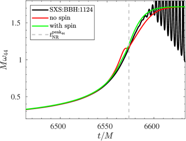
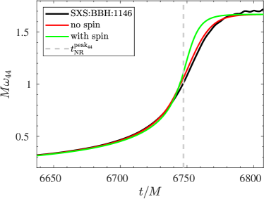
Figure 22: In this figure we compare the frequency $M\omega_{44}$ for the two NR waveforms (black) SXS:BBH:1124 $(1,0.998,0.998)$ (left panel) and SXS:BBH:1146 $(1.5,0.95,0.95)$ (right) with the corresponding EOB waveforms, once obtained using the fits of Ref. Nagar et al. (2019b) (right panel) and once with the spin-dependent fits presented in Appenix C.3 (green).

As mentioned above, the results presented in the main text do not rely on the the fits of $(c_{3}^{\phi_{33}},c_{4}^{\phi_{33}})$ and $(c_{3}^{\phi_{44}},c_{4}^{\phi_{44}})$ given in Appendix C.3 with the full spin dependence, but instead use only their spin-independent part, as already presented Ref. Nagar et al. (2019b). This choice was made so to ensure a more robust behavior of the frequency at the beginning of the ringdown when the spins are positive and large. We illustrate this argument inspecting the behavior of $\omega_{44}$ for two highly-spinning configurations. Figure 22 shows EOB/NR comparisons with two EOB waveforms obtained with either the nonspinning fits (red online) or those with the full spin dependence (green). One sees that the spin-dependent fit performs rather well for SXS:BBH:1124 $(1,0.998,0.998)$, consistently with the fact that we used SXS:BBH:0178, with parameters $(1,0.9942,0.9942)$, to inform the fit. By contrast, one sees that the same description applied to a different configuration, $(1.5,0.95,0.95)$, corresponding to SXS:BBH:1146, does not perform equally well, with a nonnegiglible gap between the EOB and NR frequencies accumulating right after the peak. One finds, however, that removing the spin-dependence in $(c_{3}^{\phi_{44}},c_{4}^{\phi_{44}})$ allows one to obtain a much closer EOB/NR consistency for SXS:BBH:1146. For the other case, moving to the nonspinning description slightly worsens the agreement, both before and after the waveform peak . On the basis of these results, and especially seen the rather good $\bar{F}$ behavior illustrated in Fig. 8, we decided to be simple and remove the spin dependence in $(c_{3}^{\phi_{44}},c_{4}^{\phi_{44}})$ . We applied the same rational also to the $(3,3)$ mode. Clearly, in case of very high-spins, currents fits should be improved to some extent, increasing the calibration set so to incorporate more points in that corner of the parameter space. This will be investigated in future work.

C.5 Modeling the NQC extraction points

Let us finally discuss analytic representations of the NR point (amplitude, frequency and derivative) on the multipolar waveform that is needed for computing the NQC corrections to the waveform multipole by multipole. For the $(2,2)$ and $(3,3)$ modes we give below dedicated fits. For all other modes, the useful NR quantities are obtained analytically from the (fitted) post-peak analytical waveform discussed above. Let us recall here that, for each mode, the NQC time is always

$$t^{\rm NQC}_{\ell m}\equiv t_{\ell m}^{\rm peak}+2.$$ (168)

All quantities mentioned below with the NQC label are computed at $t=t^{\rm NQC}_{\ell m}$.

C.5.1 The $(2,2)$ NQC extraction point

For the $(2,2)$ mode the NQC-point quantities $\left\{\hat{A}_{22}^{\rm NQC},\dot{A}_{22}^{\rm NQC},\omega_{22}^{\rm NQC},\dot{\omega}_{22}^{\rm NQC}\right\}$ are fitted directly. The 3-piece hybrid fit, presented in Nagar et al. (2017, 2018) is modified for $q>4$. The fits of $\left\{\hat{A}_{22}^{\rm NQC}\omega_{22}^{\rm NQC}\right\}$ are done using the template discussed already for the peak, see Appendix C.2.1. The reader should note however that the fit of $\omega_{22}^{\rm NQC}$ has additional flexibility. The replacement in (76) is also done for $i=2$ for this case.

Table 33: Coefficients of the $(2,2)$ quantities needed to calculate the NQC extraction point. From left to right the columns show $\left\{\hat{A}_{22}^{\rm NQC},\dot{\hat{A}}_{22}^{\rm NQC},\omega_{22}^{\rm NQC},\dot{\omega}_{22}^{\rm NQC}\right\}$.

	$\hat{A}^{\rm NQC}_{22}$			$\dot{A}^{\rm NQC}_{22}$			$\omega^{\rm NQC}_{22}$			$\dot{\omega}^{\rm NQC}_{22}$
	$\hat{A}_{22}^{{\rm NQC}_{0}}$	$=$	$\;\;\;0.294773$	$\dot{A}_{22}^{{\rm NQC}_{0}}/\nu$	$=$	$-0.000243654$	$\omega_{22}^{{\rm NQC}_{0}}$	$=$	$\;\;\;0.285588$	${\dot{\omega}_{22}^{{\rm NQC}_{0}}}$	$=$	$\;\;\;0.00628027$
	$a_{1}^{\hat{A}^{\rm NQC}_{22}}$	$=$	$-0.052697$	$a_{1}^{\dot{A}^{\rm NQC}_{22}}$	$=$	$\;\;\;2.86637$	$a_{1}^{\omega^{\rm NQC}_{22}}$	$=$	$\;\;\;0.91704$	$a_{1}^{\dot{\omega}^{\rm NQC}_{22}}$	$=$	$\;\;\;2.4351$
	$a_{2}^{\hat{A}^{\rm NQC}_{22}}$	$=$	$\;\;\;1.6088$	$a_{2}^{\dot{A}^{\rm NQC}_{22}}$	$=$	$-1.3667$	$a_{2}^{\omega^{\rm NQC}_{22}}$	$=$	$\;\;\;1.7912$	$a_{2}^{\dot{\omega}^{\rm NQC}_{22}}$	$=$	$\;\;\;4.4928$
	$b^{\hat{A}^{{\rm NQC}_{m_{1}=m_{2}}}_{22}}_{1}$	$=$	$-0.705226$	$b^{\dot{A}^{{\rm NQC}_{m_{1}=m_{2}}}_{22}}_{1}$	$=$	$\;\;\;0.02679530$	$b^{\omega^{{\rm NQC}_{m_{1}=m_{2}}}_{22}}_{1}$	$=$	$-0.46550$	$b^{\dot{\omega}^{{\rm NQC}_{m_{1}=m_{2}}}_{22}}_{1}$	$=$	$\;\;\;0.001425242$
	$b^{\hat{A}^{{\rm NQC}_{m_{1}=m_{2}}}_{22}}_{2}$	$=$	$-0.0953944$	$b^{\dot{A}^{{\rm NQC}_{m_{1}=m_{2}}}_{22}}_{2}$	$=$	$-0.0064409$	$b^{\omega^{{\rm NQC}_{m_{1}=m_{2}}}_{22}}_{2}$	$=$	$-0.078787$	$b^{\dot{\omega}^{{\rm NQC}_{m_{1}=m_{2}}}_{22}}_{2}$	$=$	$-0.00096073$
	$b^{\hat{A}^{{\rm NQC}_{m_{1}=m_{2}}}_{22}}_{3}$	$=$	$-1.087280$				$b^{\omega^{{\rm NQC}_{m_{1}=m_{2}}}_{22}}_{3}$	$=$	$-0.852284$
	$c^{\hat{A}^{{\rm NQC}}_{22}}_{11}$	$=$	$\;\;\;0.009335$	$c^{\dot{A}^{{\rm NQC}}_{22}}_{1}$	$=$	$-0.015395218$	$c^{\omega^{{\rm NQC}}_{22}}_{11}$	$=$	$-0.338008$	$c^{\dot{\omega}^{{\rm NQC}}_{22}}_{1}$	$=$	$-0.000063766$
	$c^{\hat{A}^{{\rm NQC}}_{22}}_{12}$	$=$	$\;\;\;0.582869$	$c^{\dot{A}^{{\rm NQC}}_{22}}_{2}$	$=$	$\;\;\;0.008732589$	$c^{\omega^{{\rm NQC}}_{22}}_{12}$	$=$	$\;\;\;1.077812$	$c^{\dot{\omega}^{{\rm NQC}}_{22}}_{2}$	$=$	$\;\;\;0.000513197$
							$c^{\omega^{{\rm NQC}}_{22}}_{21}$	$=$	$\;\;\;0.0555533$
							$c^{\omega^{{\rm NQC}}_{22}}_{22}$	$=$	$-0.312861$
	$c^{\hat{A}^{{\rm NQC}}_{22}}_{31}$	$=$	$\;\;\;-0.140747$				$c^{\omega^{{\rm NQC}}_{22}}_{31}$	$=$	$\;\;\;0.289185$
	$c^{\hat{A}^{{\rm NQC}}_{22}}_{32}$	$=$	$\;\;\;0.505807$				$c^{\omega^{{\rm NQC}}_{22}}_{32}$	$=$	$-0.195838$

In the following the fitting of $\dot{A}_{22}^{\rm NQC}$ and $\dot{\omega}_{22}^{\rm NQC}$. Both rely on the same template thus it is only given for the former explicitly. To fit the time derivative of the amplitude at $t_{\rm NQC}$ it was proven useful to not fit it directly, but to fit $\dot{A}_{22}^{\rm NQC}/\nu\omega_{22}^{\rm NQC}$, starting with the following factorization

$$\frac{\dot{A}_{22}^{\rm NQC}}{\nu\omega_{22}^{\rm NQC}} =\left[\hat{\dot{A}}_{22}^{{\rm NQC}_{\rm orb}}\left(\nu\right)+\hat{\dot{A}}_{22}^{{\rm NQC}_{\rm Spin}}\left(X_{12},\hat{S}\right)\right].$$ (169)

The nonspinning contribution is fitted as

$$\hat{\dot{A}}_{22}^{{\rm NQC}_{\rm orb}}\left(\nu\right)=1+a_{1}^{\dot{A}^{\rm NQC}_{22}}\nu+a_{2}^{\dot{A}^{\rm NQC}_{22}}\nu^{2}.$$ (170)

The spin-dependence is represented as

$$\hat{\dot{A}}_{22}^{{\rm NQC}_{\rm Spin}}\left(X_{12}\hat{S}\right)=b^{\dot{A}^{{\rm NQC}_{m_{1}=m_{2}}}_{22}}_{1}\hat{S}+b^{\dot{A}^{{\rm NQC}_{m_{1}=m_{2}}}_{22}}_{1}\hat{S}^{2}\,.$$ (171)

The extrapolation to the $m_{1}\neq m_{2}$ regime is done via the replacement

$$b^{\dot{A}^{{\rm NQC}_{m_{1}=m_{2}}}_{22}}_{i}\rightarrow b^{\dot{A}^{{\rm NQC}_{m_{1}=m_{2}}}_{22}}_{i}+c^{\dot{A}^{{\rm NQC}_{m_{1}=m_{2}}}_{22}}_{i}X_{12}\,,$$ (172)

with $i=\left\{1,2\right\}$. All coefficients are listed explicitly in Table 33.

C.5.2 The $(3,3)$ NQC extraction point

Let us discuss now explicit fits for $\left\{\hat{A}_{33}^{\rm NQC},\dot{A}_{33}^{\rm NQC},\omega_{33}^{\rm NQC},\dot{\omega}_{33}^{\rm NQC}\right\}$. The amplitude $\hat{A}_{33}^{\rm NQC}$ is written as two separate terms as

$$\hat{A}_{33}^{\rm NQC}=\hat{A}_{33}^{{\rm NQC}_{0}}X_{12}\hat{A}_{33}^{{\rm NQC}_{\rm orb}}(\nu)+\hat{A}_{33}^{{\rm NQC}_{\rm S}}(\nu,\tilde{a}_{12})\ ,$$ (173)

where $\hat{A}_{33}^{{\rm NQC}_{0}}$ is the test-particle value. The non-spinning sector is fitted after factorization of $\hat{A}_{33}^{{\rm NQC}_{0}}X_{12}$ with

$$\hat{A}_{33}^{{\rm NQC}_{\rm orb}}(\nu)=1+a_{1}^{\hat{A}_{33}^{{\rm NQC}}}\nu+a_{2}^{\hat{A}_{33}^{{\rm NQC}}}\nu^{2}\ .$$ (174)

The spin-dependent factor $\hat{A}_{33}^{{\rm NQC}_{\rm S}}$ is first fitted in the $\nu=0$ limit with

$$\hat{A}_{33}^{{\rm NQC}_{\rm S}}=\frac{b_{1}^{\hat{A}_{33}^{{\rm NQC}}}\tilde{a}_{12}+b_{2}^{\hat{A}_{33}^{{\rm NQC}}}\tilde{a}_{12}^{2}}{1+b_{3}^{\hat{A}_{33}^{{\rm NQC}}}\tilde{a}_{12}}\ .$$ (175)

and then extended to the $\nu\neq 0$ regime through

$$b_{i}^{\hat{A}_{33}^{{\rm NQC}}}\rightarrow\frac{b_{i}^{\hat{A}_{33}^{{\rm NQC}}}+c_{i1}^{\hat{A}_{33}^{{\rm NQC}}}\nu}{1+c_{i2}^{\hat{A}_{33}^{{\rm NQC}}}\nu}\ {\rm with}\ i=\{1,2,3\}\ .$$ (176)

The time-derivative of the amplitude $\dot{A}_{33}^{{\rm NQC}}$ was fitted in two steps. In the first step, one is fitting only equal-mass data (but, crucially, including also data with unequal spins), as

$$\frac{\dot{A}_{33}^{{\rm NQC}_{\nu=1/4}}}{10^{5}}=d_{0}^{\dot{A}_{33}^{{\rm NQC}_{\nu=1/4}}}+ d_{1}^{\dot{A}_{33}^{{\rm NQC}_{\nu=1/4}}}\tilde{a}_{12}$$

$$+d_{2}^{\dot{A}_{33}^{{\rm NQC}_{\nu=1/4}}}\tilde{a}_{12}^{2}\ .$$ (177)

The un-equal mass sector is fitted with the same template as $\hat{A}_{33}^{\rm NQC}$ with 3 modifications: (i) $X_{12}$ is not factorized as in (173); (ii) The spin variable in (175) is chosen to be $\hat{S}$; (iii) the transformation is only done for $i=2$ in (176), $c_{1i}^{\hat{A}_{33}^{{\rm NQC}}}=c_{3i}^{\hat{A}_{33}^{{\rm NQC}}}=0$.

Moving now to the NQC frequency $\omega_{33}^{\rm NQC}$, we assume the following factorization

$$\omega_{33}^{\rm NQC}=\omega_{33}^{{\rm NQC}_{0}}\omega_{33}^{{\rm NQC}_{\rm orb}}\omega_{33}^{{\rm NQC}_{\rm S}}\ ,$$ (178)

where $\omega_{33}^{{\rm NQC}_{\rm orb}}$ is fitted to the nonspinning data with a second-order polynomial in $\nu$ as

$$\omega_{33}^{{\rm NQC}_{\rm orb}}=1+a_{1}^{\omega_{33}^{{\rm NQC}}}\nu+a_{2}^{\omega_{33}^{{\rm NQC}}}\nu^{2}\ .$$ (179)

Then, $\omega_{33}^{{\rm NQC}_{\rm S}}$ if fitted to the test-particle data using

$$\omega_{33}^{{\rm NQC}_{\rm S}}=\frac{1+b_{1}^{\omega_{33}^{{\rm NQC}}}\hat{S}}{1+b_{2}^{\omega_{33}^{{\rm NQC}}}\hat{S}}\ .$$ (180)

Finally, the spin-dependence in $\omega_{33}^{{\rm NQC}_{\rm S}}$ incorporates $\nu$-dependent effects as

$$b_{i}^{\omega_{33}^{{\rm NQC}}}\rightarrow b_{i}^{\omega_{33}^{{\rm NQC}}}+c_{i}^{\omega_{33}^{{\rm NQC}}}\nu\ {\rm with}\ i=\{1,2\}\ .$$ (181)

Moving finally to the time-derivative of the frequency, $\dot{\omega}_{33}^{\rm NQC}$, it is fitted with the ansatz

$$\dot{\omega}_{33}^{\rm NQC}=\dot{\omega}_{33}^{{\rm NQC}_{0}}\dot{\omega}_{33}^{{\rm NQC}_{\rm orb}}+\dot{\omega}_{33}^{{\rm NQC}_{\rm S}}\ ,$$ (182)

where $\dot{\omega}_{33}^{{\rm NQC}_{\rm orb}}$ is fitted to nonspinning data with

$$\dot{\omega}_{33}^{{\rm NQC}_{\rm orb}}=1+a_{1}^{\dot{\omega}_{33}^{{\rm NQC}}}\nu\ .$$ (183)

$\dot{\omega}_{33}^{{\rm NQC}_{\rm S}}$ if fitted to the test-particle data with

$$\dot{\omega}_{33}^{{\rm NQC}_{\rm S}}=b_{1}^{\dot{\omega}_{33}^{{\rm NQC}}}\hat{S}+b_{2}^{\dot{\omega}_{33}^{{\rm NQC}}}\hat{S}^{2}\ .$$ (184)

The spin dependence in $\dot{\omega}_{33}^{{\rm NQC}_{\rm S}}$ is then extrapolated to the comparable mass through

$$b_{i}^{\dot{\omega}_{33}^{{\rm NQC}}}\rightarrow b_{i}^{\dot{\omega}_{33}^{{\rm NQC}}}+c_{i}^{\dot{\omega}_{33}^{{\rm NQC}}}\nu\ {\rm with}\ i=\{1,2\}\ .$$ (185)

Table 34: Coefficients of the $(3,3)$ quantities needed to calculate the NQC extraction point. From left to right the columns show $\left\{\hat{A}_{33}^{\rm NQC},\dot{\hat{A}}_{33}^{\rm NQC},\omega_{33}^{\rm NQC},\dot{\omega}_{33}^{\rm NQC}\right\}$.

	$\hat{A}^{\rm NQC}_{33}$			$\dot{A}^{\rm NQC}_{33}$			$\omega^{\rm NQC}_{33}$			$\dot{\omega}^{\rm NQC}_{33}$
	$\hat{A}_{33}^{{\rm NQC}_{0}}$	$=$	$\;\;\;0.0512928$	$\dot{A}_{33}^{{\rm NQC}_{0}}/\nu$	$=$	$-3.9568\times 10^{-4}$	$\omega_{33}^{{\rm NQC}_{0}}$	$=$	$\;\;\;0.476647$	${\dot{\omega}_{33}^{{\rm NQC}_{0}}}$	$=$	$\;\;\;0.0110394$
	$a_{1}^{\hat{A}^{\rm NQC}_{33}}$	$=$	$\;\;\;0.09537$	$a_{1}^{\dot{A}^{\rm NQC}_{33}}$	$=$	$\;\;\;1.0985$	$a_{1}^{\omega^{\rm NQC}_{33}}$	$=$	$\;\;\;1.0886$	$a_{1}^{\dot{\omega}^{\rm NQC}_{33}}$	$=$	$\;\;\;2.7962$
	$a_{2}^{\hat{A}^{\rm NQC}_{33}}$	$=$	$\;\;\;3.7217$	$a_{2}^{\dot{A}^{\rm NQC}_{33}}$	$=$	$-13.458$	$a_{2}^{\omega^{\rm NQC}_{33}}$	$=$	$\;\;\;3.0658$
	$b^{\hat{A}^{{\rm NQC}_{\nu=0}}_{33}}_{1}$	$=$	$\;\;\;0.00924494$	$b^{\dot{A}^{{\rm NQC}_{\nu=0}}_{33}}_{1}$	$=$	$\;\;\;1.41504\times 10^{-4}$	$b^{\omega^{{\rm NQC}_{\nu=0}}_{33}}_{1}$	$=$	$-0.236271$	$b^{\dot{\omega}^{{\rm NQC}_{\nu=0}}_{33}}_{1}$	$=$	$-4.5666\times 10^{-4}$
	$b^{\hat{A}^{{\rm NQC}_{\nu=0}}_{33}}_{2}$	$=$	$-8.7052\times 10^{-5}$	$b^{\dot{A}^{{\rm NQC}_{\nu=0}}_{33}}_{2}$	$=$	$\;\;\;1.04680\times 10^{-4}$	$b^{\omega^{{\rm NQC}_{\nu=0}}_{33}}_{2}$	$=$	$-0.582892$	$b^{\dot{\omega}^{{\rm NQC}_{\nu=0}}_{33}}_{2}$	$=$	$-0.00388909$
	$b^{\hat{A}^{{\rm NQC}_{\nu=0}}_{33}}_{3}$	$=$	$-0.479669$	$b^{\dot{A}^{{\rm NQC}_{\nu=0}}_{33}}_{3}$	$=$	$-0.422066$
	$c^{\hat{A}^{{\rm NQC}}_{33}}_{11}$	$=$	$\;\;\;0.0067063$	$c^{\dot{A}^{{\rm NQC}}_{33}}_{21}$	$=$	$-4.671176\times 10^{-4}$	$c^{\omega^{{\rm NQC}}_{33}}_{1}$	$=$	$-0.085544$	$c^{\dot{\omega}^{{\rm NQC}}_{33}}_{1}$	$=$	$\;\;\;0.0290846$
	$c^{\hat{A}^{{\rm NQC}}_{33}}_{12}$	$=$	$\;\;\;4.814781$	$c^{\dot{A}^{{\rm NQC}}_{33}}_{22}$	$=$	$-4.0270198$	$c^{\omega^{{\rm NQC}}_{33}}_{2}$	$=$	$-0.523365$	$c^{\dot{\omega}^{{\rm NQC}}_{33}}_{2}$	$=$	$\;\;\;0.0087659$
	$c^{\hat{A}^{{\rm NQC}}_{33}}_{21}$	$=$	$\;\;\;0.0111876$	$d_{0}^{\dot{A}_{33}^{{\rm NQC}_{\nu=1/4}}}$	$=$	$-0.090676$
	$c^{\hat{A}^{{\rm NQC}}_{33}}_{22}$	$=$	$-1.079532$	$d_{1}^{\dot{A}_{33}^{{\rm NQC}_{\nu=1/4}}}$	$=$	$-5.1643$
	$c^{\hat{A}^{{\rm NQC}}_{33}}_{31}$	$=$	$\;\;\;2.967227$	$d_{2}^{\dot{A}_{33}^{{\rm NQC}_{\nu=1/4}}}$	$=$	$-3.2594$
	$c^{\hat{A}^{{\rm NQC}}_{33}}_{32}$	$=$	$-2.571783$

C.5.3 Calculation of NQC quantities from the postpeak analytical waveform

Let us finally discuss explicitly the computation of the NQC quantities $\left(A_{\ell m}^{\rm NQC},\omega_{\ell m}^{\rm NQC},\dot{A}_{\ell m}^{\rm NQC},\dot{\omega}_{\ell m}^{\rm NQC}\right)$ from the NR-informed analytical description of the postpeak waveform, as defined in Sec. V A of Nagar et al. (2019b), to which we refer the reader for the notation. Although the formulas have to be intended valid multipole by multipole, in the following we drop the $(\ell,m)$ indexes for clarity. The analytical expression for the amplitude and its time derivative read

$$A_{h}/\nu=~{} e^{-\alpha_{1}\frac{t-t_{\rm peak}}{M_{\rm BH}}}\left[c_{1}^{A}\tanh\left(c_{2}^{A}\frac{t-t_{\rm peak}}{M_{\rm BH}}+c_{3}^{A}\right)+c_{4}^{A}\right],$$ (186)

$$\dot{A}_{h}/\nu=~{} \frac{c_{1}^{A}c^{A}_{2}e^{-\alpha_{1}\frac{t-t_{\rm peak}}{M_{\rm BH}}}{\rm sech}^{2}\left(c^{A}_{2}\frac{t-t_{\rm peak}}{M_{\rm BH}}+c^{A}_{3}\right)}{M_{\rm BH}}-\frac{\alpha_{1}e^{-\alpha_{1}\frac{t-t_{\rm peak}}{M_{\rm BH}}}\left[c^{A}_{1}\tanh\left(c^{A}_{2}\frac{t-t_{\rm peak}}{M_{\rm BH}}+c^{A}_{3}\right)+c^{A}_{4}\right]}{M_{\rm BH}},$$ (187)

while those for the phase and its derivatives read

$$\phi_{h}= -\omega_{1}\frac{t-t_{\rm peak}}{M^{2}_{\rm BH}}-c_{1}^{\phi}\mathrm{ln}\left(\frac{1+c_{3}^{\phi}e^{-c_{2}^{\phi}\frac{t-t_{\rm peak}}{M_{\rm BH}}}+c_{4}^{\phi}e^{-2c_{2}^{\phi}\frac{t-t_{\rm peak}}{M_{\rm BH}}}}{1+c_{3}^{\phi}+c_{4}^{\phi}}\right),$$ (188)

$$\omega_{h}= -\dot{\phi}_{h}\hskip 4.26773pt=\frac{\omega_{1}}{M^{2}_{\rm BH}}-\frac{c^{\phi}_{1}c^{\phi}_{2}}{M_{\rm BH}}\frac{c^{\phi}_{3}x(t)+2c^{\phi}_{4}x^{2}(t)}{1+c^{\phi}_{3}x(t)+c^{\phi}_{4}x^{2}(t)},$$ (189)

$$\dot{\omega}_{h}= -\ddot{\phi}_{h}=\frac{c^{\phi}_{1}{c^{\phi}_{2}}^{2}}{M^{2}_{\rm BH}}\left[\frac{c^{\phi}_{3}x(t)+4c^{\phi}_{4}x^{2}(t)}{1+c^{\phi}_{3}x(t)+c^{\phi}_{4}x^{2}(t)}-\left(\frac{c^{\phi}_{3}x(t)+2c^{\phi}_{4}x^{2}(t)}{1+c^{\phi}_{3}x(t)+c^{\phi}_{4}x^{2}(t)}\right)^{2}\right],$$ (190)

where we introduced

$$x(t)=e^{-c^{\phi}_{2}\frac{t-t_{\rm peak}}{M_{\rm BH}}}.$$ (191)

The waveform quantities needed to compute the NQC correction to amplitude and phase are simply obtained by evaluating the above expressions at $t=t^{\rm NQC}_{\ell m}=t_{\ell m}^{\rm peak}+2$ multipole by multipole.

C.5.4 The fitted derivative of the $(\ell,m)=(4,4)$ amplitude at the NQC extraction point

Unfortunately, we have realized that the accuracy of the derivative obtained with the above template does not always have sufficient accuracy. This is due to insufficient flexibility of the fitting template, that will be modified in future work. To overcome this difficulty, we give here an explicit fit of the amplitude time-derivative that is then used in the main text. The derivative of NQC amplitude is separated in two terms as

$$\dot{A}_{44}^{\rm NQC}=\nu\dot{A}_{44}^{{\rm NQC}_{0}}\hat{\dot{A}}_{44}^{\rm orb}(\nu)+\hat{\dot{A}}_{44}^{\rm Spin}(\hat{S},\nu)\ ,$$ (192)

where $\dot{A}_{44}^{{\rm NQC}_{0}}$ is the peak amplitude in the test particle limit. The non-spinning behavior is modeled with

$$\hat{\dot{A}}_{44}^{\rm orb}(\nu)=\frac{1+a^{\dot{A}_{44}^{\rm NQC}}_{1}\nu+a^{\dot{A}_{44}^{\rm NQC}}_{2}\nu^{2}}{1+a^{\dot{A}_{44}^{\rm NQC}}_{3}\nu+a^{\dot{A}_{44}^{\rm NQC}}_{4}\nu^{2}}\ .$$ (193)

The spin dependence is first fitted to the test-particle limit using

$$\hat{\dot{A}}_{44}^{\rm Spin}(\hat{S},\nu=0)=\frac{b^{\dot{A}_{44}^{\rm NQC}}_{1}\hat{S}}{1+b^{\dot{A}_{44}^{\rm NQC}}_{2}\hat{S}}\ ,$$ (194)

and then extrapolated to the comparable mass region through

$$b^{\dot{A}_{44}^{\rm NQC}}_{1} \rightarrow \frac{b^{\dot{A}_{44}^{\rm NQC}}_{1}+c^{\dot{A}_{44}^{\rm NQC}}_{11}\nu}{1+c^{\dot{A}_{44}^{\rm NQC}}_{12}\nu}\ ,$$ (195)

$$b^{\dot{A}_{44}^{\rm NQC}}_{2} \rightarrow \frac{b^{\dot{A}_{44}^{\rm NQC}}_{2}+c^{\dot{A}_{44}^{\rm NQC}}_{21}\nu}{1+c^{\dot{A}_{44}^{\rm NQC}}_{22}\nu}\ .$$ (196)

Table 35: Explicit coefficients of the fit of $\dot{A}_{44}^{\rm NQC}$.

	$\dot{A}_{44}^{{\rm NQC}_{0}}$	$=$	$-1.52614\times 10^{-4}$
	$a^{\dot{A}_{44}^{\rm NQC}}_{1}$	$=$	$-7.63783$
	$a^{\dot{A}_{44}^{\rm NQC}}_{2}$	$=$	$\;15.8089$
	$a^{\dot{A}_{44}^{\rm NQC}}_{3}$	$=$	$-5.88951$
	$a^{\dot{A}_{44}^{\rm NQC}}_{4}$	$=$	$\;11.1555$
	$b^{\dot{A}_{44}^{\rm NQC}}_{1}$	$=$	$\;\;\;3.76236\times 10^{-5}$
	$b^{\dot{A}_{44}^{\rm NQC}}_{2}$	$=$	$-0.819379$
	$c^{\dot{A}_{44}^{\rm NQC}}_{11}$	$=$	$-6.45958\times 10^{-6}$
	$c^{\dot{A}_{44}^{\rm NQC}}_{12}$	$=$	$-2.35613$
	$c^{\dot{A}_{44}^{\rm NQC}}_{21}$	$=$	$-298.678$
	$c^{\dot{A}_{44}^{\rm NQC}}_{22}$	$=$	$-1063.08$

References

- Aasi et al. (2015) J. Aasi et al. (LIGO Scientific), Class. Quant. Grav. 32, 074001 (2015), arXiv:1411.4547 [gr-qc] .
- Acernese et al. (2015) F. Acernese et al. (VIRGO), Class. Quant. Grav. 32, 024001 (2015), arXiv:1408.3978 [gr-qc] .
- Abbott et al. (2016a) B. P. Abbott et al. (Virgo, LIGO Scientific), Phys. Rev. Lett. 116, 061102 (2016a), arXiv:1602.03837 [gr-qc] .
- Abbott et al. (2016b) B. P. Abbott et al. (Virgo, LIGO Scientific), Phys. Rev. Lett. 116, 241103 (2016b), arXiv:1606.04855 [gr-qc] .
- Abbott et al. (2017a) B. P. Abbott et al. (VIRGO, LIGO Scientific), Phys. Rev. Lett. 118, 221101 (2017a), arXiv:1706.01812 [gr-qc] .
- Abbott et al. (2017b) B. P. Abbott et al. (Virgo, LIGO Scientific), Astrophys. J. 851, L35 (2017b), arXiv:1711.05578 [astro-ph.HE] .
- Abbott et al. (2017c) B. P. Abbott et al. (Virgo, LIGO Scientific), Phys. Rev. Lett. 119, 141101 (2017c), arXiv:1709.09660 [gr-qc] .
- Abbott et al. (2019) B. P. Abbott et al. (LIGO Scientific, Virgo), Phys. Rev. X9, 031040 (2019), arXiv:1811.12907 [astro-ph.HE] .
- Abbott et al. (2017d) B. P. Abbott et al. (Virgo, LIGO Scientific), Phys. Rev. Lett. 119, 161101 (2017d), arXiv:1710.05832 [gr-qc] .
- Abbott et al. (2020) B. Abbott et al. (LIGO Scientific, Virgo), Astrophys. J. Lett. 892, L3 (2020), arXiv:2001.01761 [astro-ph.HE] .
- O’Shaughnessy et al. (2014) R. O’Shaughnessy, B. Farr, E. Ochsner, H.-S. Cho, V. Raymond, C. Kim, and C.-H. Lee, Phys. Rev. D89, 102005 (2014), arXiv:1403.0544 [gr-qc] .
- Varma and Ajith (2017) V. Varma and P. Ajith, Phys. Rev. D96, 124024 (2017), arXiv:1612.05608 [gr-qc] .
- London et al. (2018) L. London, S. Khan, E. Fauchon-Jones, X. J. Forteza, M. Hannam, S. Husa, C. Kalaghatgi, F. Ohme, and F. Pannarale, Phys. Rev. Lett. 120, 161102 (2018), arXiv:1708.00404 [gr-qc] .
- Mehta et al. (2017) A. K. Mehta, C. K. Mishra, V. Varma, and P. Ajith, Phys. Rev. D96, 124010 (2017), arXiv:1708.03501 [gr-qc] .
- Cotesta et al. (2018) R. Cotesta, A. Buonanno, A. Bohé, A. Taracchini, I. Hinder, and S. Ossokine, Phys. Rev. D98, 084028 (2018), arXiv:1803.10701 [gr-qc] .
- Varma et al. (2019) V. Varma, S. E. Field, M. A. Scheel, J. Blackman, L. E. Kidder, and H. P. Pfeiffer, Phys. Rev. D99, 064045 (2019), arXiv:1812.07865 [gr-qc] .
- Buonanno and Damour (1999) A. Buonanno and T. Damour, Phys. Rev. D59, 084006 (1999), arXiv:gr-qc/9811091 .
- Buonanno and Damour (2000) A. Buonanno and T. Damour, Phys. Rev. D62, 064015 (2000), arXiv:gr-qc/0001013 .
- Damour et al. (2000) T. Damour, P. Jaranowski, and G. Schaefer, Phys. Rev. D62, 084011 (2000), arXiv:gr-qc/0005034 [gr-qc] .
- Damour (2001) T. Damour, Phys. Rev. D64, 124013 (2001), arXiv:gr-qc/0103018 .
- Damour et al. (2015) T. Damour, P. Jaranowski, and G. Schäfer, Phys. Rev. D91, 084024 (2015), arXiv:1502.07245 [gr-qc] .
- Bohé et al. (2017) A. Bohé et al., Phys. Rev. D95, 044028 (2017), arXiv:1611.03703 [gr-qc] .
- Ossokine et al. (2020) S. Ossokine et al., (2020), arXiv:2004.09442 [gr-qc] .
- Nagar et al. (2018) A. Nagar et al., Phys. Rev. D98, 104052 (2018), arXiv:1806.01772 [gr-qc] .
- LIGO Scientific Collaboration (2018) LIGO Scientific Collaboration, “LIGO Algorithm Library - LALSuite,” free software (GPL) (2018).
- Nagar and Rettegno (2019) A. Nagar and P. Rettegno, Phys. Rev. D99, 021501 (2019), arXiv:1805.03891 [gr-qc] .
- Akcay et al. (2019) S. Akcay, S. Bernuzzi, F. Messina, A. Nagar, N. Ortiz, and P. Rettegno, Phys. Rev. D99, 044051 (2019), arXiv:1812.02744 [gr-qc] .
- Nagar et al. (2019a) A. Nagar, F. Messina, P. Rettegno, D. Bini, T. Damour, A. Geralico, S. Akcay, and S. Bernuzzi, Phys. Rev. D99, 044007 (2019a), arXiv:1812.07923 [gr-qc] .
- Rettegno et al. (2019) P. Rettegno, F. Martinetti, A. Nagar, D. Bini, G. Riemenschneider, and T. Damour, (2019), arXiv:1911.10818 [gr-qc] .
- Nagar et al. (2019b) A. Nagar, G. Pratten, G. Riemenschneider, and R. Gamba, (2019b), arXiv:1904.09550 [gr-qc] .
- Nagar and Shah (2016) A. Nagar and A. Shah, Phys. Rev. D94, 104017 (2016), arXiv:1606.00207 [gr-qc] .
- Messina et al. (2018) F. Messina, A. Maldarella, and A. Nagar, Phys. Rev. D97, 084016 (2018), arXiv:1801.02366 [gr-qc] .
- Damour and Nagar (2014a) T. Damour and A. Nagar, Phys.Rev. D90, 044018 (2014a), arXiv:1406.6913 [gr-qc] .
- Nagar et al. (2016) A. Nagar, T. Damour, C. Reisswig, and D. Pollney, Phys. Rev. D93, 044046 (2016), arXiv:1506.08457 [gr-qc] .
- Damour and Nagar (2014b) T. Damour and A. Nagar, Phys.Rev. D90, 024054 (2014b), arXiv:1406.0401 [gr-qc] .
- Del Pozzo and Nagar (2017) W. Del Pozzo and A. Nagar, Phys. Rev. D95, 124034 (2017), arXiv:1606.03952 [gr-qc] .
- Nagar et al. (2017) A. Nagar, G. Riemenschneider, and G. Pratten, Phys. Rev. D96, 084045 (2017), arXiv:1703.06814 [gr-qc] .
- Boyle et al. (2019) M. Boyle et al., Class. Quant. Grav. 36, 195006 (2019), arXiv:1904.04831 [gr-qc] .
- Damour et al. (2009) T. Damour, B. R. Iyer, and A. Nagar, Phys. Rev. D79, 064004 (2009), arXiv:0811.2069 [gr-qc] .
- Pan et al. (2011) Y. Pan, A. Buonanno, R. Fujita, E. Racine, and H. Tagoshi, Phys.Rev. D83, 064003 (2011), arXiv:1006.0431 [gr-qc] .
- Nagar et al. (2019c) A. Nagar, F. Messina, C. Kavanagh, G. Lukes-Gerakopoulos, N. Warburton, S. Bernuzzi, and E. Harms, Phys. Rev. D100, 104056 (2019c), arXiv:1907.12233 [gr-qc] .
- Damour et al. (2013) T. Damour, A. Nagar, and S. Bernuzzi, Phys.Rev. D87, 084035 (2013), arXiv:1212.4357 [gr-qc] .
- Fujita (2015) R. Fujita, PTEP 2015, 033E01 (2015), arXiv:1412.5689 [gr-qc] .
- Harms et al. (2014) E. Harms, S. Bernuzzi, A. Nagar, and A. Zenginoglu, Class.Quant.Grav. 31, 245004 (2014), arXiv:1406.5983 [gr-qc] .
- (45) “SXS Gravitational Waveform Database,” https://data.black-holes.org/waveforms/index.html.
- Buchman et al. (2012) L. T. Buchman, H. P. Pfeiffer, M. A. Scheel, and B. Szilagyi, Phys. Rev. D86, 084033 (2012), arXiv:1206.3015 [gr-qc] .
- Chu et al. (2009) T. Chu, H. P. Pfeiffer, and M. A. Scheel, Phys. Rev. D80, 124051 (2009), arXiv:0909.1313 [gr-qc] .
- Hemberger et al. (2013) D. A. Hemberger, G. Lovelace, T. J. Loredo, L. E. Kidder, M. A. Scheel, B. Szilágyi, N. W. Taylor, and S. A. Teukolsky, Phys. Rev. D88, 064014 (2013), arXiv:1305.5991 [gr-qc] .
- Scheel et al. (2015) M. A. Scheel, M. Giesler, D. A. Hemberger, G. Lovelace, K. Kuper, M. Boyle, B. Szilágyi, and L. E. Kidder, Class. Quant. Grav. 32, 105009 (2015), arXiv:1412.1803 [gr-qc] .
- Blackman et al. (2015) J. Blackman, S. E. Field, C. R. Galley, B. Szilágyi, M. A. Scheel, M. Tiglio, and D. A. Hemberger, Phys. Rev. Lett. 115, 121102 (2015), arXiv:1502.07758 [gr-qc] .
- Lovelace et al. (2012) G. Lovelace, M. Boyle, M. A. Scheel, and B. Szilagyi, Class. Quant. Grav. 29, 045003 (2012), arXiv:1110.2229 [gr-qc] .
- Lovelace et al. (2011) G. Lovelace, M. Scheel, and B. Szilagyi, Phys.Rev. D83, 024010 (2011), arXiv:1010.2777 [gr-qc] .
- Lovelace et al. (2015) G. Lovelace et al., Class. Quant. Grav. 32, 065007 (2015), arXiv:1411.7297 [gr-qc] .
- Mroue et al. (2013) A. H. Mroue, M. A. Scheel, B. Szilagyi, H. P. Pfeiffer, M. Boyle, et al., Phys.Rev.Lett. 111, 241104 (2013), arXiv:1304.6077 [gr-qc] .
- Kumar et al. (2015) P. Kumar, K. Barkett, S. Bhagwat, N. Afshari, D. A. Brown, G. Lovelace, M. A. Scheel, and B. Szilágyi, Phys. Rev. D92, 102001 (2015), arXiv:1507.00103 [gr-qc] .
- Chu et al. (2016) T. Chu, H. Fong, P. Kumar, H. P. Pfeiffer, M. Boyle, D. A. Hemberger, L. E. Kidder, M. A. Scheel, and B. Szilagyi, Class. Quant. Grav. 33, 165001 (2016), arXiv:1512.06800 [gr-qc] .
- (57) “Updated Advanced LIGO sensitivity design curve,” https://dcc.ligo.org/LIGO-T1800044/public.
- Khan et al. (2016) S. Khan, S. Husa, M. Hannam, F. Ohme, M. Pürrer, X. Jiménez Forteza, and A. Bohé, Phys. Rev. D93, 044007 (2016), arXiv:1508.07253 [gr-qc] .
- (59) D. Shoemaker, https://dcc.ligo.org/cgi-bin/DocDB/ShowDocument?docid=2974 .
- Baiotti et al. (2010) L. Baiotti, T. Damour, B. Giacomazzo, A. Nagar, and L. Rezzolla, Phys. Rev. Lett. 105, 261101 (2010), arXiv:1009.0521 [gr-qc] .
- Baiotti et al. (2011) L. Baiotti, T. Damour, B. Giacomazzo, A. Nagar, and L. Rezzolla, Phys. Rev. D84, 024017 (2011), arXiv:1103.3874 [gr-qc] .
- Taracchini et al. (2014) A. Taracchini, A. Buonanno, G. Khanna, and S. A. Hughes, Phys.Rev. D90, 084025 (2014), arXiv:1404.1819 [gr-qc] .
- (63) https://bitbucket.org/eob_ihes/teobresums/src/master/, TEOBResumS code.
- (64) G. Riemenschneider, P. Rettegno, and A. Nagar, in preparation, 2020 .
- Husa et al. (2016) S. Husa, S. Khan, M. Hannam, M. Pürrer, F. Ohme, X. Jiménez Forteza, and A. Bohé, Phys. Rev. D93, 044006 (2016), arXiv:1508.07250 [gr-qc] .
- Keitel et al. (2017) D. Keitel et al., Phys. Rev. D96, 024006 (2017), arXiv:1612.09566 [gr-qc] .
- Jiménez-Forteza et al. (2017) X. Jiménez-Forteza, D. Keitel, S. Husa, M. Hannam, S. Khan, and M. Pürrer, Phys. Rev. D95, 064024 (2017), arXiv:1611.00332 [gr-qc] .