The Energy Sources of Double-peaked superluminous supernova PS1-12cil and luminous supernova SN 2012aa

Abstract

In this paper, we present the study for the energy reservoir powering the light curves (LCs) of PS1-12cil and SN 2012aa which are superluminous and luminous supernovae (SNe), respectively. The multi-band and bolometric LCs of these two SNe show unusual secondary bumps after the main peaks. The two-peaked LCs cannot be explained by any simple energy-source models (e.g., the ⁵⁶Ni cascade decay model, the magnetar spin-down model, and the ejecta-circumstellar medium interaction model). Therefore, we employ the ⁵⁶Ni plus ejecta-circumstellar medium (CSM) interaction (CSI) model, the magnetar plus CSI model, and the double CSI model to fit their bolometric LCs, and find that both these two SNe can be explained by the double CSI model and the magnetar plus CSI model. Based on the modeling, we calculate the the time when the shells were expelled by the progenitors: provided that they were powered by double ejecta-shell CSI, the inner and outer shells might be expelled $\sim 0.2-3.6$ and $\sim 2-25$ years before the explosions of the SNe, respectively; the shells were expelled $\sim 2-20$ years before the explosions of the SNe if they were powered by magnetars plus CSI.

1 Introduction

Supernovae (SNe) are energetic explosions emitting luminous ultraviolet (UV), optical, and near infrared (NIR) radiation. The peak luminosities of most of SNe are $\sim 10^{42}-10^{43}$ erg s^-1. According to the spectra around the light-curves (LCs) peaks, SNe can be divided into types I which are hydrogen-deficient and II which are hydrogen-rich (Minkowski, 1941). Type I SNe can be divided into types Ia, Ib, and Ic, while most of type II SNe can be divided into types II-P, II-L, IIn, and IIb. (Filippenko, 1997). The spectral types directly reflects the properties of the progenitors of SNe. It has long been believed that type Ia SNe result from the explosions of white drawfs (Hoyle & Fowler, 1960), while the other types of SNe come from collapse of massive stars (Baade & Zwicky, 1934; Janka et al., 2016).

SNe Ic have attracted more and more attention due partly to the fact that a fraction of them have been found to be associated with long gamma-ray bursts (GRBs) (e.g., Galama et al. 1998; Hjorth et al. 2003, see Woosley & Bloom 2006; Cano et al. 2017 for reviews). On the other hand, over 100 superluminous SNe (SLSNe) whose peak luminosities are $\sim$ 100 times brighter than that of normal SNe have been discovered and studied in the past two decades(Gal-Yam, 2012; Inserra, 2019); meanwhile, dozens of luminous optical transients (including luminous SNe) with peak luminosities between that of normal and superluminous SNe have also been discovered (Arcavi et al., 2016). Like normal SNe, SLSNe and luminous SNe can also be classified into types I and II and most of SLSNe I are SNe Ic.

Previous research have shown that the LCs of almost all ordinary SNe can be explained by the ⁵⁶Ni model and the hydrogen recombination model while the LCs of almost all SLSNe and luminous SNe cannot be explained by the ⁵⁶Ni model. Alternatively, the magnetar spin-down model (Kasen & Bildsten, 2010; Inserra et al., 2013; Nicholl et al., 2013, 2014; Wang et al., 2015b, 2016a), the ejecta-circumstellar medium (CSM) interaction (CSI) model (Chevalier, 1982; Chevalier & Fransson, 1994; Chevalier & Irwin, 2011; Chatzopoulos et al., 2012; Liu et al., 2018), and the fallback model (Dexter & Kasen, 2013) have been employed to account for the LCs of SLSNe, some luminous SNe as well as a fraction of rapid rising luminous optical transients (see, Moriya et al. 2018; Wang et al. 2019; Inserra 2019 for reviews and references therein).

Nevertheless, all energy-source models mentioned above (the ⁵⁶Ni model, the magnetar model, the CSI model and the fallback model) cannot reproduce the LCs of SNe showing two or more peaks, (e.g. iPTF13ehe, Yan et al. 2015; iPTF15esb, Yan et al. 2017; PTF12dam, and iPTF13dcc, Vreeswijk et al. 2017). To resolve this problem, various models have been developed. Piro (2015) develop a semi-analytic post-shock cooling model that can be used to account for the first peak of the LC of a double-peaked SN and the second peak of the SN can be explained by the aforementioned models. Wang et al. (2016b) propose that a double energy source model (magnetar plus CSI) or a triple energy source model (⁵⁶Ni plus magnetar plus CSI) can be used to explain the LCs of SLSNe exhibiting a rebrightening or double-peaked feature; Vreeswijk et al. (2017) suggest that a cooling plus magnetar model can explain the LCs of PTF12dam and iPTF13dcc; Liu et al. (2018) develop a multiple CSI model involving the collisions between the ejecta and the CSM shells or winds locating at different sites and use these models to fit the LCs of iPTF15esb and iPTF13dcc.

In this paper, we study two hydrogen-poor SNe, PS1-12cil and SN 2012aa. PS1-12cil is a SLSN I discovered by the Panoramic Survey Telescope $\&$ Rapid Response System (Pan-STARRS1, PS1; Kaiser et al. 2010; Tonry et al. 2012) Medium Deep Survey (PS1 MDS) at a redshift ($z$) of 0.32 (Lunnan et al., 2018); SN 2012aa is a luminous SN Ic that was discovered by the Lick Observatory Supernova Search (LOSS, Filippenko et al. 2001) at a redshift ($z$) of 0.083 (Roy et al., 2016). The multi-band LCs of these two SNe show unusual post-peak bumps (Lunnan et al., 2018; Roy et al., 2016) and make them double-peaked SNe which cannot be explained by any models that can reproduce single-peak LCs. We research the possible energy sources that can account for the double-peaked LCs of PS1-12cil and SN 2012aa and constrain the physical parameters of the models. In Section 2, we use the ⁵⁶Ni plus CSI model, the magnetar plus CSI model, and the multiple CSI model to fit the bolometric LCs of PS1-12cil and SN 2012aa and derive the best-fitting parameters. Our discussion and conclusions can be found in Sections 3 and 4, respectively.

2 Modeling the Bolometric LCs of PS1-12cil and SN 2012aa

In their paper, Roy et al. (2016) employ the ⁵⁶Ni model and the magnetar model to model the bolometric LC of SN 2012aa. It can be found that while the first peak and the late-time LC of SN 2012aa can be well fit by these two models, the second peak, i.e., the post-peak bump cannot be explained by these models. More complicated models are needed to resolve this problem. Roy et al. (2016) suggest that ⁵⁶Ni plus CSI model might be a reasonable model to account for the whole double-peaked LC of SN 2012aa, but they don’t model the LC using this model. Similarly, the double-peaked LC of PS1-12cil must be modelled by more complicated models rather than simpler models like the ⁵⁶Ni model and the magnetar model. Therefore, we don’t consider these simple models throughout this paper.

In this section, we reproduce the bolometric LCs of PS1-12cil and SN 2012aa by adopting the ⁵⁶Ni plus CSI model, the magnetar plus CSI model, and the multiple CSI model. Markov Chain Monte Carlo (MCMC) technique is employed to obtain the best-fitting parameters and the 1$\sigma$ uncertainties.

2.1 The ⁵⁶Ni Plus CSI Model

Firstly, we employ the ⁵⁶Ni plus CSI model to fit the bolometric LCs of PS1-12cil and SN 2012aa. We suppose that the ⁵⁶Ni power the first peaks, while the second peaks (bumps) can be explained by the CSI model. The ⁵⁶Ni model in our double-energy-source model including following parameters: the optical opacity $\kappa$, the ejecta mass $M_{\rm{ej}}$, the mass of ⁵⁶Ni $M_{\mathrm{Ni}}$, the gamma-ray opacity of of ⁵⁶Ni decay photons $\kappa_{\gamma,\mathrm{Ni}}$, the moment of explosion $t_{\rm{expl}}$, the velocity of the ejecta $v_{\rm{SN}}$. Based on their photospheric velocity from (Lunnan et al., 2018) and (Roy et al., 2016), the velocities of the ejecta of PS1-12cil and SN 2012aa are set to be $15,000\ \rm{km\ s^{-1}}$ and $11,400\ \rm{km\ s^{-1}}$, respectively.

The density profile of the inner regions and the outer regions of the ejecta can be described by $\rho_{\rm{ej}}\propto R_{\rm ej}^{-\delta}$ and $\rho_{\rm{ej}}\propto R_{\rm ej}^{-n}$ (here, we take $\delta=0$ and $n=7$), respectively; the density profile of the CSM can be described by $\rho_{\rm CSM}\propto R_{\rm CSM}^{-s}$ ($s=0$ for material shells, $s=2$ for stellar winds). Forward shock and reverse shock generated by the interactions between the ejecta and CSM propagate into CSM and ejecta, respectively, converting the kinetic energy to radiation and driving the LCs of the bumps.

The parameters of the CSI model are the CSM mass $M_{\rm{CSM}}$, the density of the innermost part of the CSM $\rho_{\rm{CSM,in}}$, the efficiency of conversion from the kinetic energy to radiation $\epsilon$, the dimensionless position parameter of break in the ejecta from the inner region to the outer region $x_{\rm{0}}$, the trigger moment of the interactions $t_{\rm{CSI}}$, and $M_{\rm{ej}}$.

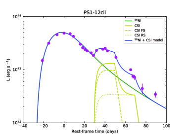
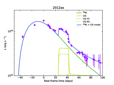
Figure 1: The bolometric LCs of PS1-12cil (left panel) and SN 2012aa (right panel) reproduced by the ⁵⁶Ni plus CSI model. Data are taken from Lunnan et al. (2018) and Roy et al. (2016), respectively. The abscissa represents time since the explosion in the rest frame.

The theoretical bolometric LCs reproduced by the ⁵⁶Ni plus CSI model are shown in Figure 1. It can be found that the theoretical LCs can match the observational data. For PS1-12cil, the masses of the ejecta, ⁵⁶Ni, and CSM are $M_{\rm{ej}}=4.95_{-0.73}^{+0.76}\rm\ M_{\odot}$, $M_{\rm{Ni}}=3.57_{-0.06}^{+0.07}\rm\ M_{\odot}$, $M_{\rm{CSM}}=4.66_{-0.70}^{+0.76}\rm\ M_{\odot}$, respectively; for SN 2012aa, the masses of the ejecta, ⁵⁶Ni, and CSM are $M_{\rm{ej}}=5.89_{-0.12}^{+0.12}\rm\ M_{\odot}$, $M_{\rm{Ni}}=1.63_{-0.01}^{+0.01}\rm\ M_{\odot}$, $M_{\rm{CSM}}=1.47_{-0.09}^{+0.15}\rm\ M_{\odot}$. These three parameters and other best-fit parameters are listed in Table 1.

2.2 The Magnetar Plus CSI Model

Replacing the mass of ⁵⁶Ni $M_{\mathrm{Ni}}$ and the gamma-ray opacity of of ⁵⁶Ni decay photons $\kappa_{\gamma,\mathrm{Ni}}$ by the magnetic field strength $B_{p}$, the initial spin periods $P_{0}$, and the gamma-ray opacity of magnetar spinning-down generated photons $\kappa_{\gamma,\rm{mag}}$, the ⁵⁶Ni plus CSI model can be changed to the magnetar plus CSI model. Here, we use this model to fit the LCs of For PS1-12cil and SN 2012aa.

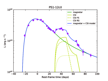
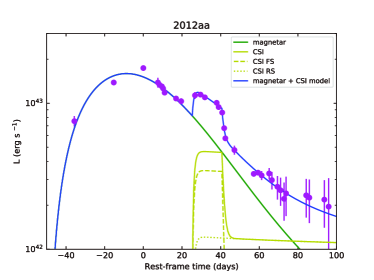
Figure 2: The bolometric LCs of PS1-12cil (left panel) and SN 2012aa (right panel) reproduced by the magnetar plus CSI model. Data are taken from Lunnan et al. (2018) and Roy et al. (2016), respectively. The abscissa represents time since the explosion in the rest frame.

The theoretical LCs yielded by the magnetar plus CSI model are plotted in Figure 2. They also match the observational data. For PS1-12cil, the best-fitting parameters are: $M_{\rm{ej}}=10.59_{-3.37}^{+3.25}\rm\ M_{\odot}$, $P_{0}=6.52_{-0.10}^{+0.09}\rm\ ms$, $B_{p}=5.09_{-0.13}^{+0.13}\times 10^{14}\rm\ G$, $M_{\rm{CSM}}=9.64_{-3.04}^{+2.97}\rm\ M_{\odot}$; for SN 2012aa, the best-fitting parameters are: $M_{\rm{ej}}=10.28_{-0.61}^{+0.72}\rm\ M_{\odot}$, $P_{0}=8.99_{-0.14}^{+0.11}\rm\ ms$, $B_{p}=4.68_{-0.29}^{+0.40}\times 10^{14}\rm\ G$, $M_{\rm{CSM}}=1.93_{-0.12}^{+0.15}\rm\ M_{\odot}$. These four parameters and other best-fit parameters are listed in Table 2.

2.3 The Multiple CSI Model

The multiple CSI model developed by Liu et al. (2018) is also a promising model that can account for two or more LC peaks of SNe. The free parameters of multiple CSI model are listed in 3. Based on the shapes of bolometric LCs of PS1-12cil and SN 2012aa, we assume that there are two interactions between ejecta and CSM. In other words, the multiple CSI model adopted here is a double CSI model. It is reasonable to suppose that the outer CSM are shells ($s=0$) while the inner CSM can either be the stellar wind ($s=2$) or the shell ($s=0$). Both these two combinations are considered here.

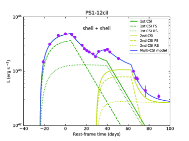
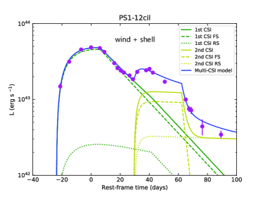
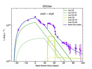
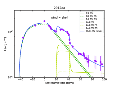
Figure 3: The bolometric LCs of PS1-12cil (top panels) and SN 2012aa (bottom panels) reproduced by the double CSI model. The left panels represent the double shell ($s=0$) case, while the right panels represent the wind ($s=2$) plus shell ($s=0$) case. Data are taken from Lunnan et al. (2018) and Roy et al. (2016), respectively. The abscissa represents time since the explosion in the rest frame.

The LCs produced by the double CSI model are shown in Figure 3 and the best-fitting parameters are listed in Table 3. For PS1-12cil, $M_{\rm{ej},1}=25.64_{-3.12}^{+2.51}\rm\ M_{\odot}$, $M_{\rm{CSM},1}=17.19_{-1.88}^{+1.59}\rm\ M_{\odot}$, $M_{\rm{CSM},2}=4.07_{-0.51}^{+0.65}\rm\ M_{\odot}$ if the inner CSM is a wind ($s=2$); otherwise ($s=0$), $M_{\rm{ej},1}=13.18_{-2.07}^{+2.56}\rm\ M_{\odot}$, $M_{\rm{CSM},1}=7.13_{-1.15}^{+1.39}\rm\ M_{\odot}$, $M_{\rm{CSM},2}=6.26_{-0.97}^{+0.93}\rm\ M_{\odot}$. For SN 2012aa, $M_{\rm{ej},1}=19.46_{-1.25}^{+1.70}\rm\ M_{\odot}$, $M_{\rm{CSM},1}=19.41_{-0.65}^{+0.37}\rm\ M_{\odot}$, $M_{\rm{CSM},2}=2.36_{-0.17}^{+0.15}\rm\ M_{\odot}$ if the the inner CSM is a wind ($s=2$); otherwise ($s=0$), $M_{\rm{ej},1}=15.60_{-0.97}^{+0.93}\rm\ M_{\odot}$, $M_{\rm{CSM},1}=17.77_{-0.96}^{+0.95}\rm\ M_{\odot}$, $M_{\rm{CSM},2}=2.16_{-0.19}^{+0.20}\rm\ M_{\odot}$.

3 Discussion

3.1 Which is the Best Model?

3.1.1 PS1-12cil

For PS1-12cil, the ⁵⁶Ni plus CSI model is disfavored since the ratio of the mass of ⁵⁶Ni ($3.57_{-0.06}^{+0.07}\rm\ M_{\odot}$) to the mass of the eject ($4.95_{-0.73}^{+0.76}\rm\ M_{\odot}$) $M_{\rm{Ni}}/M_{\rm{ej}}$ is $\sim 0.72$ while the upper limit of this ratio is $\sim 0.2$ (Umeda & Nomoto, 2008) and Inserra et al. (2013) suggest that 0.5 can be regarded as the upper limit of this ratio.

The theoretical LC yielded by the magnetar plus CSI model can match the data well and the value of $\chi^{2}/\rm{dof}$ of this model is $54.39/11=4.94$.

For the two shell CSI model, the masses of the inner shell ($M_{\rm{CSM},1}$) and the outer shell ($M_{\rm{CSM},2}$) are $\sim 7.13\rm\ M_{\odot}$) and $\sim 6.26\rm\ M_{\odot}$, respectively; the value of $\chi^{2}/\rm{dof}$ of this model is $21.08/10=2.11$.

For the case of the “inner wind plus outer shell” combination, the value of $\chi^{2}/\rm{dof}$ of this model is $31.48/10=3.15$. Assuming that the velocity of the wind of the progenitor of an SN Ibc is ($v_{\rm w}$) is $100-1000\rm\ km\ s^{-1}$ (see, e.g., Table 1 of Smith 2014), the mass loss rate $\dot{M}=4\pi v_{\rm w}q$ ($q=\rho_{\rm CSM,in,1}R_{\rm CSM,in,1}^{2}$) of the stellar wind is $\dot{M}\sim 10.1-101\ \rm M_{\odot}\ yr^{-1}$, significantly larger than the typical values for most of SN progenitors.

To produce such extreme wind mass loss, so-called “super-winds” are required. Recently, Moriya et al. (2019) suggest that the multi-peaked IIP SN iPTF14hls is a optical transient powered by mass loss history. In this scenario, the maximum mass loss rate must be larger than 10 $\rm M_{\odot}$ yr ^-1. As pointed out by Moriya et al. (2019), however, how to produce so large mass loss is unclear. Moreover, the velocity of the putative wind of PS1-12cil might be significantly larger than 100 $\rm km~{}s^{-1}$ and can be up to 1000 $\rm km~{}s^{-1}$ since PS1-12cil is a hydrogen-poor SLSN whose progenitor might be a Wolf-Rayet-like star which would blow high-velocity wind; in this case, the mass loss rate would be significantly larger than 10 $\rm M_{\odot}$ yr ^-1. Therefore, the scenario involving a wind with mass loss rate $\gtrsim$ 10 $\rm M_{\odot}$ yr ^-1 need some unknown extraordinary mechanism.

Comparing the $\chi^{2}/\rm{dof}$ of these models, the double CSI model involving two shells ($s=0$) is the best one for PS1-12cil, while the magnetar plus CSI model is also a promising model that can account for the LC of PS1-12cil.

The spectral features would provide more information. The PS1-12cil’s spectrum obtained 1 day after the peak don’t show emission line due to the the CSI, indicating either that the early LC of PS1-12cil might be powered by the magnetar rather than CSI or that the CSM is asymmetric and the emission lines were swallowed by the ejecta. There are no late-time spectra and the power sources powering the late-time LC cannot be constrained by spectra. If we neglect the asymmetry effect, the magnetar plus CSI model is the best one.

3.1.2 SN 2012aa

For SN 2012aa, the value of $\chi^{2}/\rm{dof}$ of the ⁵⁶Ni plus CSI model is $92.90/22=4.22$. The model need $1.63_{-0.01}^{+0.01}\rm\ M_{\odot}$ of ⁵⁶Ni; the ejecta mass derived is $5.89_{-0.12}^{+0.12}\rm\ M_{\odot}$, indicating that the value of $M_{\rm{Ni}}/M_{\rm{ej}}$ is $\sim 0.28$. This value is larger than 0.2 but smaller than 0.5, so the ⁵⁶Ni plus CSI model cannot be completely excluded.

Based on the parameters derived, the value of the kinetic energy of SN 2012aa can be calculated, $\sim 4.6\times 10^{51}$ erg, which is lower than those of some hypernovae ($\gtrsim 10^{52}$ erg, e.g., SNe 1998bw and 2003dh), suggesting that the mass of ⁵⁶Ni must be lower than those of these hypernovae for which the inferred ⁵⁶Ni masses are $\lesssim 0.5\rm\ M_{\odot}$. However, the ⁵⁶Ni mass derived by ⁵⁶Ni plus CSI model is $1.63_{-0.01}^{+0.01}\rm\ M_{\odot}$, significantly higher than those of SNe 1998bw and 2003dh. So this model is disfavored.

The values of the parameters of the magnetar plus CSI model are reasonable, and the value of $\chi^{2}/\rm{dof}$ of this model is $36.77/21=1.75$. For the two shell CSI model, the masses of the inner shell ($M_{\rm{CSM},1}$) and the outer shell ($M_{\rm{CSM},2}$) are $\sim 18\rm\ M_{\odot}$) and $\sim 2\rm\ M_{\odot}$, respectively; the value of $\chi^{2}/\rm{dof}$ of this model is $18.61/20=0.93$. For wind plus shell CSI model, the derived value of $\dot{M}$ is $\sim 10.4-104\ \rm M_{\odot}\ yr^{-1}$, and the value of $\chi^{2}/\rm{dof}$ of this model is $44.23/20=2.21$.

So the two shell CSI model is the best one for SN 2012aa and the magnetar plus CSI model is also a reasonable model in explaining the SN 2012aa’s LC.

The early spectra of SN 2012aa resemble those of SNe Ic-BL, Roy et al. (2016) point out that the broad emission feature (Gaussian FWHM $\approx 14,000\rm~{}km~{}s^{-1}$) near H$\alpha$ remains almost constant throughout its evolution. This feature is prominent in the spectrum 47 d after the LC peak of SN 2012aa. Roy et al. (2016) suggest that this feature could be due to [O I] $\lambda\lambda$6300, 6364 or blueshifted (1500-2500 $\rm kms^{-1}$) H$\alpha$ emission.

For the latter explanation, Roy et al. (2016) propose that the feature is consistent with the CSM-interaction scenario since it becomes prominent by +47 d when the LC peaks again. If the early-time LC was also powered by CSI, the possible emission lines associated with CSI might be stronger than that in the late-time spectra since the density and mass of the inner shell are larger than those of outer shell, inconsistent with the observations which show that the feature was marginally present in the spectrum by +29 d and become prominent in the spectrum +47 d. Therefore, the magnetar plus CSI model is favored.

Nevertheless, if the broad emission feature is [O I] $\lambda\lambda$6300, 6364 rather than the CSI-induced emission lines, we can expect that the CSI between the ejecta and the asymmetric CSM could produce the CSI without emission lines. In this case, both the two shell CSI model and the magnetar plus CSI model are plausible.

3.2 The the Mass Loss Histories of PS1-12cil and SN 2012aa

The most promising models of PS1-12cil and SN 2012aa is the two shell CSI model. However, the magnetar plus CSI model is also a possible model for these two SNe. It is interesting to infer the mass-loss histories of these two SNe based on these two models.

Provided that ${\Delta}t^{\prime}$ is the interval between the time when the shells were expelled and the time when the shells were collided, ${\Delta}t=t_{\mathrm{CSI}}-t_{\mathrm{expl}}$ is the interval between the time when the SNe exploded and the time when the shells were collided, we have $v_{\rm SN}{\Delta}t=v_{\rm shell}({\Delta}t^{\prime}+{\Delta}t)$, i.e., ${\Delta}t^{\prime}=(v_{\rm SN}/v_{\rm shell}-1){\Delta}t$, here, $v_{\rm shell}$ is the velocity of the shells. Supposing that the value of the velocity of the shells is $100-1000\rm\ km\ s^{-1}$, we can infer the values of $t^{\prime}$.

Under the hypothesis that the LCs of PS1-12cil and SN 2012aa were powered by two shell CSI, the values of of $t^{\prime}$ can be derived below. For PS1-12cil, $v_{\rm SN}=15,000\ \rm{km\ s^{-1}}$, ${\Delta}t_{\rm inner}\sim 8.70$ days, ${\Delta}t_{\rm inner}^{\prime}\sim 121.74-1295.70$ days ($\sim 0.3-3.6$ years); ${\Delta}t_{\rm outer}\sim 62.14$ days, ${\Delta}t_{\rm outer}^{\prime}\sim 869.90-9258.26$ days ($\sim 2.4-25.4$ years). For SN 2012aa, $v_{\rm SN}=11,400\ \rm{km\ s^{-1}}$, ${\Delta}t_{\rm inner}\sim 8.27$ days, ${\Delta}t_{\rm inner}^{\prime}\sim 86.05-935.01$ days ($\sim 0.2-2.6$ years); ${\Delta}t_{\rm outer}\sim 79.08$ days, ${\Delta}t_{\rm outer}^{\prime}\sim 822.48-8936.54$ days ($\sim 2.3-24.5$ years). We find that the values of ${\Delta}t^{\prime}$ of the inner shells of these two SNe are approximately equal to each other; similarly, the values of ${\Delta}t^{\prime}$ of the outer shells of these two SNe are also approximately equal to each other.

Similarly, we can infer the values of of $t^{\prime}$ based on the assumption that these two SNe were powered by magnetars and CSI. For PS1-12cil, $v_{\rm SN}=15,000\ \rm{km\ s^{-1}}$, ${\Delta}t\sim 55$ days, then ${\Delta}t^{\prime}\sim 770-8200$ days, $\sim 2-22$ years. For SN 2012aa, $v_{\rm SN}=11,400\ \rm{km\ s^{-1}}$, ${\Delta}t\sim 75$ days, then ${\Delta}t^{\prime}\sim 780-8500$ days, $\sim 2-23$ years. The values of ${\Delta}t^{\prime}$ of these two SNe are equal to each other.

3.3 Comparing the Properties of these two SNe and other double-peaked SNe associated with CSI

It is interesting to compare the observation properties and the derived physical parameters of these two SNe. From the observational aspect, both two SNe have bright main-peaks, and the delay time between the main-peaks and the bumps (second peaks) are about 40 days, indicating that the model parameters might be rather similar if they share the same origin.

If we suppose that the first peaks of these two SNe were powered by the magnetars, the initial spin periods ($P_{0}$) and the magnetic field strength ($B_{p}$) of the putative magnetars are $\sim 7-10$ ms and $\sim 5\times 10^{14}$ G, respectively. These values are consistent with that of the magnetars supposed to power the LCs of type I SLSNe (Liu et al., 2017; Yu et al., 2017; Nicholl et al., 2017). Moreover, the CSM shells should be expelled $\sim 2-22$ years prior to the SN explosions if the post-peak bumps were powered by the CSI.

Provided that the whole LCs of PS1-12cil and SN 2012aa were powered by two shell CSI, we find that the mass loss histories of inner shells ($\sim 0.3-3$ years prior to the SN explosions) and the outer shells ($\sim 2-25$ years prior to the SN explosions) of these two SNe are also approximately equal to each other.

The resemblances between these two SNe suggest that the properties of their progenitors are similar to each other: they yield magnetars with nearly same properties and experience the same pre-SN eruptions for in the magnetar plus CSI scenario, or experience the two pre-SN eruptions sharing the properties consistent with each other.

Furthermore, we can compare these two SNe with other double-peaked SNe which have $\sim 40$ days delay between two peaks. Smith et al. (2014a) suggest that both SN 2009ip (2012a/b, Mauerhan et al. 2013; Pastorello et al. 2013; Margutti et al. 2014; Smith et al. 2010) and SN 2010mc (Ofek et al., 2013; Smith et al., 2014b) are double-peaked SNe whose second peaks are powered by CSI. Smith et al. (2014a) suggest that the first peaks with absolute magnitudes $\sim-15$ mag were powered by the ⁵⁶Ni decay while the second peaks $\sim 3$ mag brighter than the first peaks were powered by CSI. The delay between the two first and second peaks of the two SNe studied are also $\sim$ 40 days, nearly identical to those of PS1-12cil and SN 2012aa. Supposing that the first peaks of PS1-12cil and SN 2012aa were powered by magnetars and the the first peaks of SN 2009ip and SN 2010mc while the second peaks of the four SNe were powered by CSI, the resemblances between the observations of these four SNe indicate that they might have similar pre-SN mass loss histories.

While the delay between the first and second peaks of these four SNe are $\sim 40$ days, there are some discrepancy between their observation features. First, the first peaks of SN 2009ip and SN 2010mc are $\sim 3$ magnitude dimmer than the second peaks; in contrast, the first peaks of PS1-12cil and SN 2012aa are brighter than the second peaks. This discrepancy might be due to the different energy sources: the first peaks of SN 2009ip and SN 2010mc have been believed to be powered by ⁵⁶Ni decay and the first peaks of PS1-12cil and SN 2012aa might be powered by CSI or magnetars. Moreover, the r/R-band absolute magnitudes of the first peaks of PS1-12cil and SN 2012aa are respectively $\sim-21$ mag (derived by combining the Figure 2 of Lunnan et al. 2018 and PS1-12cil’s redshift, 0.32) and $\sim-20$ mag (Roy et al., 2016), at least $2-3$ magnitude brighter than the first peaks of SN 2009ip and SN 2010mc.

Both SN 2012aa and SN 2009ip locate at the outskirts of their host galaxies (the values for PS1-12cil and SN 2010mc have not been confirmed): the distance between SN 2012aa and the galaxy center is $\sim$3 kpc, while the distance between SN 2009ip and the galaxy center is $\sim 5$ kpc which is larger than that of the former. The properties of the host galaxies and their location are also rather different: the host of SN 2012aa is a normal star-forming galaxy with solar metallicity, while the host of SN 2010mc is a faint low-metallicity dwarf galaxy.

3.4 Can the Cooling Emission Plus ⁵⁶Ni/Magnetar Explain the LCs of PS1-12cil and SN 2012aa

The post-shock cooling emission plus ⁵⁶Ni/magnetar are also plausible models that can account for some double-peaked SNe. However, the cooling emission would power monotonically decreasing bolometric LCs (see, e.g., Piro 2015) that don’t have rising parts. In contrast, the LCs around the first peaks of bolometric LCs of PS1-12cil and SN 2012aa shown clear rising phases. Therefore, the models involving cooling emission are disfavored.

A shock breakout plus cooling emission may reproduce rising and descending peak, but its rising phase is too short to compatible with the bolometric LCs of PS1-12cil and SN 2012aa.

4 Conclusions

PS1-12cil is a Type I SLSN, while SN 2012aa is a luminous Type Ic SN. The bolometric LCs of these two SNe are double-peaked and cannot be explained by any models that can reproduce single-peaked LCs. In this paper, We use three models, the ⁵⁶Ni plus CSI model, the magnetar plus CSI model, and the double CSI model, to account for their bolometric LCs.

According to the best-fitting parameters and the physical constraints, we find that the two shell CSI model is the most promising one that can reproduce the bolometric LCs of these two SNe. For PS1-12cil, the model parameters are $M_{\rm{ej}}=13.18_{-2.07}^{+2.56}\rm\ M_{\odot}$, $M_{\rm{CSM,1}}=7.13_{-1.15}^{+1.39}\rm\ M_{\odot}$, and $M_{\rm{CSM,2}}=6.26_{-0.97}^{+0.93}\rm\ M_{\odot}$ For SN 2012aa, the model parameters are $M_{\rm{ej}}=15.60_{-0.97}^{+0.93}\rm\ M_{\odot}$, $M_{\rm{CSM,1}}=17.77_{-0.96}^{+0.95}\rm\ M_{\odot}$, and $M_{\rm{CSM,2}}=2.16_{-0.19}^{+0.20}\rm\ M_{\odot}$.

The magnetar plus CSI model is also a good model to fit the LCs of these two SNe. For PS1-12cil, the model parameters are $M_{\rm{ej}}=10.59_{-3.37}^{+3.25}\rm\ M_{\odot}$, $P_{0}=6.52_{-0.10}^{+0.09}\rm\ ms$, $B_{p}=5.09_{-0.13}^{+0.13}\times 10^{14}\rm\ G$, and $M_{\rm{CSM}}=9.64_{-3.04}^{+2.97}\rm\ M_{\odot}$. For SN 2012aa, the model parameters are $M_{\rm{ej}}=10.28_{-0.61}^{+0.72}\rm\ M_{\odot}$, $P_{0}=8.99_{-0.14}^{+0.11}\rm\ ms$, $B_{p}=4.68_{-0.29}^{+0.40}\times 10^{14}\rm\ G$, and $M_{\rm{CSM}}=1.93_{-0.12}^{+0.15}\rm\ M_{\odot}$.

Based on the explosion time $t_{\mathrm{expl}}$ and the collision time $t_{\mathrm{CSI}}$ between the ejecta and the CSM, we can infer the mass loss histories of the progenitors. Provided that they were powered by double ejecta-shell CSI, the inner and outer shells were expelled $\sim 0.2-3.6$ and $\sim 2-25$ years before the explosions of the SNe, respectively; the shells were expelled $\sim 2-20$ years before the explosions of the SNe if they were powered by magnetars plus CSI.

The precursor eruption events have been observed (see, e.g., Ofek et al. 2014a; Arcavi et al. 2017) in the images obtained several years or several decades before the detections of the corresponding SNe II/IIn. Furthermore, Yan et al. (2015) estimated that at least 15$\%$ of SLSNe-I might expel precursor eruptions before the SN explosions; the interactions between SN ejecta and the CSM would power a late-time LC rebrightening and the SNe would be confirmed as the double- or multiple-peaked SNe if the late-time follow-up can be conducted successfully.

Researching the properties of the LCs of some double- or multi-peaked SNe would provide useful information about the precursor eruptions. It can be expected that future optical sky-survey telescopes would discover more double- or multi-peaked SNe and the theoretical studies would yield more valuable conclusions.

Table 1: Parameters of the ⁵⁶Ni plus CSI model. The uncertainties are 1$\sigma$.

	$\kappa$	$M_{\mathrm{ej}}$	$M_{\mathrm{Ni}}$	$M_{\mathrm{CSM}}$	$\rho_{\mathrm{CSM,in}}$	$\epsilon$	$x_{\mathrm{0}}$	$\kappa_{\gamma,\mathrm{Ni}}$	$t_{\mathrm{expl}}$	$t_{\mathrm{CSI}}$	$\chi^{2}/\mathrm{dof}$
	(cm2 g-1)	(M⊙)	(M⊙)	(M⊙)	($10^{-12}$g cm-3)			(cm2 g-1)	(days)	(days)
PS1-12cil	$0.14_{-0.02}^{+0.03}$	$4.95_{-0.73}^{+0.76}$	$3.57_{-0.06}^{+0.07}$	$4.66_{-0.70}^{+0.76}$	$21.47_{-8.16}^{+7.58}$	$0.43_{-0.11}^{+0.11}$	$0.11_{-0.01}^{+0.02}$	$0.01_{-0.01}^{+0.02}$	$-27.95_{-0.21}^{+0.22}$	$29.16_{-0.42}^{+0.34}$	$60.45/12$
2012aa	$0.20_{-0.00}^{+0.00}$	$5.89_{-0.12}^{+0.12}$	$1.63_{-0.01}^{+0.01}$	$1.47_{-0.09}^{+0.15}$	$2.14_{-0.85}^{+2.24}$	$0.51_{-0.16}^{+0.14}$	$0.11_{-0.01}^{+0.02}$	$0.01_{-0.01}^{+0.01}$	$-46.46_{-0.47}^{+0.45}$	$24.72_{-5.22}^{+0.82}$	$92.90/22$

Table 2: Parameters of the magnetar plus CSI model. The uncertainties are 1$\sigma$.

	$\kappa$	$M_{\mathrm{ej}}$	$P_{0}$	$B_{p}$	$M_{\mathrm{CSM}}$	$\rho_{\mathrm{CSM,in}}$	$\epsilon$	$x_{\mathrm{0}}$	$\kappa_{\gamma,\mathrm{mag}}$	$t_{\mathrm{expl}}$	$t_{\mathrm{CSI}}$	$\chi^{2}/\mathrm{dof}$
	(cm2 g-1)	(M⊙)	(ms)	($10^{14}$ G)	(M⊙)	($10^{-12}$g cm-3)			(cm2 g-1)	(days)	(days)
PS1-12cil	$0.08_{-0.02}^{+0.04}$	$10.59_{-3.37}^{+3.25}$	$6.52_{-0.10}^{+0.09}$	$5.09_{-0.13}^{+0.13}$	$9.64_{-3.04}^{+2.97}$	$56.09_{-21.01}^{+22.04}$	$0.18_{-0.05}^{+0.11}$	$0.12_{-0.01}^{+0.01}$	$2.72_{-0.40}^{+16.94}$	$-26.24_{-0.21}^{+0.20}$	$28.64_{-0.21}^{+0.30}$	$54.39/11$
2012aa	$0.19_{-0.01}^{+0.01}$	$10.28_{-0.61}^{+0.72}$	$8.99_{-0.14}^{+0.11}$	$4.68_{-0.29}^{+0.40}$	$1.93_{-0.12}^{+0.15}$	$4.24_{-2.42}^{+1.91}$	$0.29_{-0.10}^{+0.07}$	$0.12_{-0.01}^{+0.03}$	$0.01_{-0.01}^{+0.01}$	$-49.91_{-0.62}^{+0.83}$	$25.32_{-0.35}^{+0.31}$	$36.77/21$

Table 3: Parameters of the double CSI model. The uncertainties are 1$\sigma$.

	$i$th	$s$	$\kappa$	$M_{\mathrm{ej},i}$	$M_{\mathrm{CSM},i}$	$R_{\mathrm{CSM,in},i}$	$\epsilon_{i}$	$\rho_{\mathrm{CSM,in},i}$	$x_{\mathrm{0}}$	$t_{\mathrm{CSI},i}$	$\chi^{2}/\mathrm{dof}$
	Interaction		(cm2 g-1)	(M⊙)	(M⊙)	($10^{14}$cm)		($10^{-12}$g cm-3)		(days)
PS1-12cil	1	0	$0.16_{-0.02}^{+0.02}$	$13.18_{-2.07}^{+2.56}$	$7.13_{-1.15}^{+1.39}$	$11.27_{-6.47}^{+9.31}$	$0.56_{-0.10}^{+0.14}$	$7.04_{-2.29}^{+3.03}$	$0.14_{-0.01}^{+0.01}$	$-24.46_{-0.27}^{+0.30}$	$21.08/10$
	2	0		$20.30$	$6.26_{-0.97}^{+0.93}$	$80.53$	$0.14_{-0.02}^{+0.04}$	$1.60_{-0.37}^{+0.25}$		$28.98_{-0.30}^{+0.38}$
	1	2	$0.15_{-0.01}^{+0.02}$	$25.64_{-3.12}^{+2.51}$	$17.19_{-1.88}^{+1.59}$	$8.36_{-1.60}^{+1.71}$	$0.69_{-0.11}^{+0.12}$	$7.23_{-2.17}^{+3.74}$	$0.11_{-0.01}^{+0.01}$	$-23.86_{-0.20}^{+0.20}$	$31.48/10$
	2	0		$42.84$	$4.07_{-0.51}^{+0.65}$	$77.32$	$0.27_{-0.04}^{+0.05}$	$0.72_{-0.24}^{+0.33}$		$29.35_{-0.56}^{+0.35}$
2012aa	1	0	$0.19_{-0.01}^{+0.01}$	$15.60_{-0.97}^{+0.93}$	$17.77_{-0.96}^{+0.95}$	$8.15_{-3.99}^{+4.22}$	$0.30_{-0.02}^{+0.02}$	$18.19_{-1.71}^{+1.12}$	$0.14_{-0.00}^{+0.00}$	$-45.74_{-0.65}^{+0.61}$	$18.61/20$
	2	0		$33.36$	$2.16_{-0.19}^{+0.20}$	$77.91$	$0.11_{-0.01}^{+0.01}$	$1.21_{-0.29}^{+0.28}$		$25.07_{-0.50}^{+0.39}$
	1	2	$0.19_{-0.01}^{+0.00}$	$19.46_{-1.25}^{+1.70}$	$19.41_{-0.65}^{+0.37}$	$19.79_{-2.34}^{+1.70}$	$0.74_{-0.15}^{+0.09}$	$1.33_{-0.26}^{+0.36}$	$0.11_{-0.01}^{+0.01}$	$-43.28_{-0.60}^{+0.60}$	$44.23/20$
	2	0		$38.87$	$2.36_{-0.17}^{+0.15}$	$81.39$	$0.23_{-0.05}^{+0.03}$	$1.13_{-0.35}^{+0.31}$		$19.26_{-0.10}^{+0.10}$

References

- Arcavi et al. (2016) Arcavi, I., Wolf, W. M., Howell, D. A., et al. 2016, ApJ, 819, 35
- Arcavi et al. (2017) Arcavi, I., Howell, D. A., Kasen, D., et al. 2017, Nature, 551, 210
- Baade & Zwicky (1934) Baade, W., & Zwicky, F. 1934, Proceedings of the National Academy of Science, 20, 254
- Cano et al. (2017) Cano, Z., Wang, S.-Q., Dai, Z.-G., & Wu, X.-F. 2017, Advances in Astronomy, 2017, 8929054
- Chatzopoulos et al. (2012) Chatzopoulos, E., Wheeler, J. C., & Vinko, J. 2012, ApJ, 746, 121
- Chevalier (1982) Chevalier, R. A. 1982, ApJ, 258, 790
- Chevalier & Fransson (1994) Chevalier, R. A., & Fransson, C. 1994, ApJ, 420, 268
- Chevalier & Irwin (2011) Chevalier, R. A., & Irwin, C. M. 2011, ApJ, 729, L6
- Chugai & Danziger (2003) Chugai, N. N., & Danziger, I. J. 2003, Astronomy Letters, 29, 649
- Chugai et al. (2004) Chugai, N. N., Blinnikov, S. I., Cumming, R. J., et al. 2004, MNRAS, 352, 1213
- Dexter & Kasen (2013) Dexter, J., & Kasen, D. 2013, ApJ, 772, 30
- Filippenko (1997) Filippenko, A. V. 1997, ARA&A, 35, 309
- Filippenko et al. (2001) Filippenko, A. V., Li, W. D., Treffers, R. R., & Modjaz, M. 2001, in Astronomical Society of the Pacific Conference Series, Vol. 246, IAU Colloq. 183: Small Telescope Astronomy on Global Scales, ed. B. Paczynski, W.-P. Chen, & C. Lemme, 121
- Fransson et al. (2014) Fransson, C., Ergon, M., Challis, P. J., et al. 2014, ApJ, 797, 118
- Gal-Yam (2012) Gal-Yam, A. 2012, Science, 337, 927
- Galama et al. (1998) Galama, T. J., Vreeswijk, P. M., van Paradijs, J., et al. 1998, Nature, 395, 670
- Hjorth et al. (2003) Hjorth, J., Sollerman, J., Møller, P., et al. 2003, Nature, 423, 847
- Hoyle & Fowler (1960) Hoyle, F., & Fowler, W. A. 1960, ApJ, 132, 565
- Inserra (2019) Inserra, C. 2019, Nature Astronomy, 3, 697
- Inserra et al. (2013) Inserra, C., Smartt, S. J., Jerkstrand, A., et al. 2013, ApJ, 770, 128
- Janka et al. (2016) Janka, H.-T., Melson, T., & Summa, A. 2016, Annual Review of Nuclear and Particle Science, 66, 341
- Kaiser et al. (2010) Kaiser, N., Burgett, W., Chambers, K., et al. 2010, in Society of Photo-Optical Instrumentation Engineers (SPIE) Conference Series, Vol. 7733, Proc. SPIE, 77330E
- Kasen & Bildsten (2010) Kasen, D., & Bildsten, L. 2010, ApJ, 717, 245
- Liu et al. (2018) Liu, L.-D., Wang, L.-J., Wang, S.-Q., & Dai, Z.-G. 2018, ApJ, 856, 59
- Liu et al. (2017) Liu, L.-D., Wang, S.-Q., Wang, L.-J., et al. 2017, ApJ, 842, 26
- Lunnan et al. (2018) Lunnan, R., Chornock, R., Berger, E., et al. 2018, ApJ, 852, 81
- Margutti et al. (2014) Margutti, R., Milisavljevic, D., Soderberg, A. M., et al. 2014, ApJ, 780, 21
- Mauerhan et al. (2013) Mauerhan, J. C., Smith, N., Filippenko, A. V., et al. 2013, MNRAS, 430, 1801
- Mazzali et al. (2013) Mazzali, P. A., Walker, E. S., Pian, E., et al. 2013, MNRAS, 432, 2463
- Minkowski (1941) Minkowski, R. 1941, PASP, 53, 224
- Moriya et al. (2019) Moriya, T. J., Mazzali, P. A., & Pian, E. 2019, MNRAS, 2714
- Moriya et al. (2018) Moriya, T. J., Sorokina, E. I., & Chevalier, R. A. 2018, Space Sci. Rev., 214, 59
- Nicholl et al. (2017) Nicholl, M., Guillochon, J., & Berger, E. 2017, ApJ, 850, 55
- Nicholl et al. (2013) Nicholl, M., Smartt, S. J., Jerkstrand, A., et al. 2013, Nature, 502, 346
- Nicholl et al. (2014) —. 2014, MNRAS, 444, 2096
- Nyholm et al. (2017) Nyholm, A., Sollerman, J., Taddia, F., et al. 2017, A&A, 605, A6
- Ofek et al. (2013) Ofek, E. O., Sullivan, M., Cenko, S. B., et al. 2013, Nature, 494, 65
- Ofek et al. (2014a) Ofek, E. O., Sullivan, M., Shaviv, N. J., et al. 2014a, ApJ, 789, 104
- Ofek et al. (2014b) Ofek, E. O., Zoglauer, A., Boggs, S. E., et al. 2014b, ApJ, 781, 42
- Pastorello et al. (2013) Pastorello, A., Cappellaro, E., Inserra, C., et al. 2013, ApJ, 767, 1
- Piro (2015) Piro, A. L. 2015, ApJ, 808, L51
- Roy et al. (2016) Roy, R., Sollerman, J., Silverman, J. M., et al. 2016, A&A, 596, A67
- Smith (2013) Smith, N. 2013, MNRAS, 429, 2366
- Smith (2014) —. 2014, ARA&A, 52, 487
- Smith et al. (2014a) Smith, N., Mauerhan, J. C., & Prieto, J. L. 2014a, MNRAS, 438, 1191
- Smith et al. (2014b) —. 2014b, MNRAS, 438, 1191
- Smith et al. (2012) Smith, N., Silverman, J. M., Filippenko, A. V., et al. 2012, AJ, 143, 17
- Smith et al. (2010) Smith, N., Miller, A., Li, W., et al. 2010, AJ, 139, 1451
- Smith et al. (2011) Smith, N., Li, W., Miller, A. A., et al. 2011, ApJ, 732, 63
- Stoll et al. (2011) Stoll, R., Prieto, J. L., Stanek, K. Z., et al. 2011, ApJ, 730, 34
- Tonry et al. (2012) Tonry, J. L., Stubbs, C. W., Lykke, K. R., et al. 2012, ApJ, 750, 99
- Umeda & Nomoto (2008) Umeda, H., & Nomoto, K. 2008, ApJ, 673, 1014
- Vreeswijk et al. (2017) Vreeswijk, P. M., Leloudas, G., Gal-Yam, A., et al. 2017, ApJ, 835, 58
- Wang et al. (2016a) Wang, L.-J., Wang, S. Q., Dai, Z. G., et al. 2016a, ApJ, 821, 22
- Wang et al. (2016b) Wang, S. Q., Liu, L. D., Dai, Z. G., Wang, L. J., & Wu, X. F. 2016b, ApJ, 828, 87
- Wang et al. (2019) Wang, S. Q., Wang, L. J., & Dai, Z. G. 2019, Research in Astronomy and Astrophysics, 19, 063
- Wang et al. (2015a) Wang, S. Q., Wang, L. J., Dai, Z. G., & Wu, X. F. 2015a, ApJ, 807, 147
- Wang et al. (2015b) —. 2015b, ApJ, 799, 107
- Woosley & Bloom (2006) Woosley, S. E., & Bloom, J. S. 2006, ARA&A, 44, 507
- Yan et al. (2015) Yan, L., Quimby, R., Ofek, E., et al. 2015, ApJ, 814, 108
- Yan et al. (2017) Yan, L., Lunnan, R., Perley, D. A., et al. 2017, ApJ, 848, 6
- Yu et al. (2017) Yu, Y.-W., Zhu, J.-P., Li, S.-Z., Lü, H.-J., & Zou, Y.-C. 2017, ApJ, 840, 12
- Zhang et al. (2012) Zhang, T., Wang, X., Wu, C., et al. 2012, AJ, 144, 131