Angular momentum profiles of Class 0 protostellar envelopes

Abstract

Context. Understanding the initial properties of star forming material and how they affect the star formation process is a key question. The infalling gas must redistribute most of its initial angular momentum inherited from prestellar cores before reaching the central stellar embryo. Disk formation has been naturally considered as a possible solution to this ”angular momentum problem”. However, how the initial angular momentum of protostellar cores is distributed and evolves during the main accretion phase and the beginning of disk formation has largely remained unconstrained up to now.

Aims. In the framework of the IRAM CALYPSO survey, we obtained observations of the dense gas kinematics that we used to quantify the amount and distribution of specific angular momentum at all scales in collapsing-rotating Class 0 protostellar envelopes.

Methods. We used the high dynamic range C¹⁸O (2$-$1) and N₂H⁺ (1$-$0) datasets to produce centroid velocity maps and probe the rotational motions in the sample of 12 envelopes from scales $\sim$50 to $\sim$5000 au.

Results. We identify differential rotation motions at scales $\lesssim$1600 au in 11 out of the 12 protostellar envelopes of our sample by measuring the velocity gradient along the equatorial axis, which we fit with a power-law model $\mathrm{v}\propto r^{\alpha}$. This suggests that coherent motions dominate the kinematics in the inner protostellar envelopes. The radial distributions of specific angular momentum in the CALYPSO sample suggest the following two distinct regimes within protostellar envelopes: the specific angular momentum decreases as $j\propto r^{1.6\pm 0.2}$ down to $\sim$1600 au and then tends to become relatively constant around $\sim$6 $\times$ 10^-4 km s^-1 pc down to $\sim$50 au.

Conclusions. The values of specific angular momentum measured in the inner Class 0 envelopes suggest that material directly involved in the star formation process ($<$1600 au) has a specific angular momentum on the same order of magnitude as what is inferred in small T-Tauri disks. Thus, disk formation appears to be a direct consequence of angular momentum conservation during the collapse. Our analysis reveals a dispersion of the directions of velocity gradients at envelope scales $>$1600 au, suggesting that these gradients may not be directly related to rotational motions of the envelopes. We conclude that the specific angular momentum observed at these scales could find its origin in other mechanisms, such as core-forming motions (infall, turbulence), or trace an imprint of the initial conditions for the formation of protostellar cores.

1 Introduction

Stars form via the gravitational collapse of $\lesssim 0.1$ pc dense cores, which are embedded within molecular clouds (André et al., 2000; Ward-Thompson et al., 2007; di Francesco et al., 2007). Prestellar cores become unstable and collapse due to their own gravitational potential. One or several stellar embryos form in their center. This is the beginning of the main accretion phase called the protostellar phase. Observations of the molecular line emission from large samples of cores in close star-forming regions revealed that velocity gradients are ubiquitous to prestellar structures at scales of 0.1$-$0.5 pc (Goodman et al., 1993; Caselli et al., 2002). These were interpreted as slow rotation inherited from their formation process (Goodman et al., 1993; Caselli et al., 2002; Ohashi et al., 1999; Redman et al., 2004; Williams et al., 2006). Assuming these gradients trace organized rotational motions, the observed velocities lead to a typical angular rotation velocity of $\Omega\sim$ 2 km s^-1 pc^-1 and specific angular momentum values of $j=\rm{v}\times r\sim 10^{-3}-10^{-1}$ km s^-1 pc.

During the collapse, if the angular momentum of the parent prestellar cores is totally transferred to the stellar embryo, the gravitational force can not counteract the centrifugal force and the stellar embryo fragments prematurely before reaching the main sequence. This is the angular momentum problem for star formation (Bodenheimer, 1995). Although observational studies suggest a trend of decreasing specific angular momentum toward smaller core sizes of $j\propto r^{1.6}$, the $j$ measured in prestellar structures at scales of 10000 au ($\sim 10^{-3}$ km s^-1 pc, Caselli et al. 2002) is still typically three orders of magnitude higher than the one associated with the maximum rotational energy that a solar-type star can sustain ($j_{\mathrm{break}}\sim$ 10¹⁸ cm² s^-1 $\sim$ 3 $\times$10^-6 km s^-1 pc). The physical mechanisms responsible for the angular momentum redistribution before the matter is accreted by the central stellar object have still to be identified.

During the star formation process, disk formation is expected to be a consequence of angular momentum conservation during the collapse of rotating cores (Cassen & Moosman, 1981; Terebey et al., 1984). From observational studies, disks are common in Class II objects (Andrews et al., 2009; Isella et al., 2009; Ricci et al., 2010; Spezzi et al., 2013; Piétu et al., 2014; Cieza et al., 2019). Thus, disk formation has been naturally considered as a possible solution to the angular momentum problem by redistributing the four orders of magnitude of $j$ measured from prestellar cores to the T-Tauri stars ($j\sim$2 $\times$10^-7 km s^-1 pc, Bouvier et al. 1993): the disk would store and evacuate the angular momentum of the matter by viscous friction (Lynden-Bell & Pringle, 1974; Hartmann et al., 1998; Najita & Bergin, 2018) or thanks to disk winds (Blandford & Payne, 1982; Pelletier & Pudritz, 1992; Pudritz et al., 2007) before the matter is accreted by the central stellar object. However, the spatial distribution of angular momentum during disk formation within star-forming structures at scales between the outer core radius and the stellar surface are still largely unconstrained.

Class 0 protostars are the first (proto)stellar objects observed after the collapse in prestellar cores (André et al., 1993, 2000). Due to their youth, most of their mass is still in the form of a dense, collapsing, reservoir envelope surrounding the central stellar embryo (M${}_{\mathrm{env}}\gg$ M_⋆). Thus, they are likely to retain the initial conditions inherited from prestellar cores, in particular regarding angular momentum. The young stellar embryo mass increases via the accretion of the gaseous and dusty envelope in a short timescale ($t<$10⁵ yr, Evans et al. 2009; Maury et al. 2011). During this main accretion phase, most of the final stellar mass is accreted and, at the same time, the infalling gas must redistribute most of its initial angular momentum before reaching the central stellar embryo. Class 0 protostars are therefore key objects to understand the distribution of angular momentum of the material directly involved in the star formation process and constrain physical mechanisms responsible for the redistribution as disk formation.

Clear signatures of rotation (Belloche et al., 2002; Belloche & André, 2004; Chen et al., 2007) and infalling gas are generally detected in the envelopes of Class 0 protostars (see the review by Ward-Thompson et al. 2007). Thanks to observations of the dense molecular gas emission, rotational motions where characterized in seven Class 0 or I protostellar envelopes at scales between 3500 and 10000 au (Ohashi et al., 1997b; Belloche et al., 2002; Chen et al., 2007). These envelopes exhibit an average angular momentum of $\sim$10^-3 km s^-1 pc at scales of $r<$5000 au, consistent with the $j$ measured in prestellar cores by Caselli et al. (2002) ($\sim 10^{-3}$ km s^-1 pc). These studies suggest an angular momentum that is constant with radius in Class 0 protostellar envelopes. These flat profiles are generally interpreted as the conservation of the angular momentum. From hydrodynamical simulations, the conservation of these typical values of angular momentum results in the formation of large rotationally supported disks with radii $>$100 au in a few thousand years (Yorke & Bodenheimer, 1999). However, from observational studies, large disks are rare around Class 0 protostars (r$<$100 au, Maury et al. 2010; Kurono et al. 2013; Yen et al. 2013; Segura-Cox et al. 2016; Maury et al. 2019). Only recent numerical simulations including magnetohydrodynamics and non-ideal effects, such as ambipolar diffusion, Ohmic dissipation, or the Hall effect, allow small rotationally supported disks to be formed ($<$100 au; Machida et al. 2014; Tsukamoto et al. 2015; Masson et al. 2016).

Very few studies have been able to produce resolved profiles of angular momentum to characterize the actual amount of angular momentum present at the smallest scales ($r\lesssim$1000 au) within protostellar envelopes. From interferometric observations, Yen et al. (2015a) derive specific angular momentum values of $\sim$2 $\times$10^-4 km s^-1 pc in seven Class 0 envelopes at scales of $r\sim$1000 au, values which are below the trend observed by Ohashi et al. (1997b). These studies have put constraints on the angular momentum properties of Class 0 protostellar envelopes and suggest the material at $r\sim$1000 au must reduce its angular momentum by at least one order of magnitude from outer envelope to disk scales. Yen et al. (2011, 2017) show specific angular momentum profiles down to $\sim$350 au in two Class 0 protostellar envelopes: $j\sim$ 6 $\times$10^-4 km s^-1 pc at $r\sim$1000 au and $j\lesssim$10^-4 km s^-1 pc at $r\sim$350 au. In this case, conservation of angular momentum during rotating protostellar collapse might not be the dominant process leading to the formation of disks and stellar multiple systems. It is therefore crucial to obtain robust estimates of the angular momentum of the infalling material in protostellar envelopes during the main accretion phase by analyzing the kinematics from the outer regions of the envelope (10000 au, Motte & André 2001) to the protostellar disk ($<$50 au, Maury et al. 2019).

2 The CALYPSO survey

The Continuum And Lines in Young ProtoStellar Objects (CALYPSO) IRAM Large Program is a survey of 16 nearby Class 0 protostars (d$<$450 pc), carried out with the IRAM Plateau de Bure interferometer (PdBI) and IRAM 30-meter telescope (30m) at wavelengths of 1.29, 1.37, and 3.18 mm. The CALYPSO sources are among the youngest known solar-type Class 0 objects (André et al., 2000) with envelope masses of $M_{\mathrm{env}}\sim$1.5 $M_{\odot}$ and internal luminosities of $L_{\mathrm{bol}}\sim$0.1$-$30 $L_{\odot}$ (Maury et al., 2019).

The CALYPSO program allows us to study in detail the Class 0 envelope chemistry (Maury et al., 2014; Anderl et al., 2016; De Simone et al., 2017; Belloche et al., 2020), disk properties (Maret et al., 2014; Maury et al., 2019; Maret et al., 2020) and protostellar jets (Codella et al. 2014a; Santangelo et al. 2015; Podio et al. 2016; Lefèvre et al. 2017; Anderl et al. subm.; Podio et al. in prep.). One of the main goals of this large observing program is to understand how the circumstellar envelope is accreted onto the central protostellar object during the Class 0 phase, and ultimately tackle the angular momentum problem of star formation. This paper presents an analysis of envelope kinematics, for the 12 sources from the CALYPSO sample located at $d\leq$350 pc (see Table 2) and discuss our results on the properties of the angular momentum in Class 0 protostellar envelopes.

We adopt the dust continuum peak at 1.3 mm (225 GHz) determined from the PdBI datasets by Maury et al. (2019) as origin of the coordinate offsets of the protostellar envelopes (see Table 2). We report for each source in Table 2 the outflow axis considered as the rotation axis and estimated by Podio & CALYPSO (in prep.) from high-velocity emission of ¹²CO, SiO, and SO at scales $<$10^′′. We assume the equatorial axis of the protostellar envelopes, namely the intersection of the equatorial plane with the plane of the sky at the distance of the source, to be perpendicular to the rotation axis. The SiO emission in the CALYPSO maps is very collimated, so the uncertainties on the direction of the rotation axis, and thus on the direction of the equatorial axis, are smaller than $\pm$10^∘ (Podio & CALYPSO, in prep.). For L1521-F, IRAM04191, and GF9-2, no collimated SiO jet is detected, thus, the uncertainties are a bit larger ($\pm$20^∘). We also use estimates of the inclination of the equatorial plane with respect to the line of sight from the literature. These estimates, which come from geometric models that best reproduce the outflow kinematics observed in molecular emission, are highly uncertain since we do not have access to the 3D-structure of each source.

Table 1: Sample of CALYPSO Class 0 protostars considered for this analysis.

Source	R.A. (J2000)	DEC (J2000)	$d$	$L_{\mathrm{int}}$	$M_{\mathrm{env}}$	$R_{\mathrm{env}}$	PA outflow	$i$	Refs
	(h:m:s)	(∘:$\arcmin$:′′)	(pc)	($L_{\mathrm{\odot}}$)	($M_{\mathrm{\odot}}$)	(au)	(∘)	(∘)
L1448-2A1	03:25:22.405	30:45:13.26	293	4.7	1.9	5300	-63 (blue), +140 (red)	30 $\pm$ 10	1, 2, 3, 4
L1448-2A2	03:25:22.355	30:45:13.16
L1448-NB1	03:25:36.378	30:45:14.77	293	3.9	4.8	9700	-80	30 $\pm$ 15	5, 6, 7, 4-8
L1448-NB2	03:25:36.315	30:45:15.15
L1448-C	03:25:38.875	30:44:05.33	293	10.9	2.0	7300	-17	20 $\pm$ 5	9, 6, 7, 10-11
IRAS2A	03:28:55.570	31:14:37.07	293	47	7.9	10000	+205	30 $\pm$ 15	12, 13, 7, 14-15
SVS13-B	03:29:03.078	31:15:51.74	293	3.1	2.8	2100	+167	30 $\pm$ 20	16, 17, 3, …
IRAS4A1	03:29:10.537	31:13:30.98	293	4.7	12.3	1700	+180	15 $\pm$ 10	12, 6, 3, 18
IRAS4A2	03:29:10.432	31:13:32.12
IRAS4B	03:29:12.016	31:13:08.02	293	2.3	4.7	3200	+167	20 $\pm$ 15	12, 6, 7, 19
IRAM04191	04:21:56.899	15:29:46.11	140	0.05	0.5	14000	+20	40 $\pm$ 10	20, 21, 7, 22
L1521F	04:28:38.941	26:51:35.14	140	0.035	0.7$-$2	4500	+240	20 $\pm$ 20	23, 24, 3, 25
L1527	04:39:53.875	26:03:09.66	140	0.9	1.2	17000	+90	3 $\pm$ 5	26, 7, 7, 25
L1157	20:39:06.269	68:02:15.70	352	4.0	3.0	15800	+163	10 $\pm$ 10	27, 7, 7, 28-29
GF9-2	20:51:29.823	60:18:38.44	200	0.3	0.5	7000	0	30 $\pm$ 20	30, 31, 3, …

(1) O’Linger et al. (1999); (2) Enoch et al. (2009); (3) Maury et al. (2019); (4) Tobin et al. (2007); (5) Curiel et al. (1990); (6) Sadavoy et al. (2014); (7) Motte & André (2001); (8) Kwon et al. (2006); (9) Anglada et al. (1989); (10) Bachiller et al. (1995); (11) Girart & Acord (2001); (12) Jennings et al. (1987); (13) Karska et al. (2013); (14) Codella et al. (2004); (15) Maret et al. (2014); (16) Grossman et al. (1987); (17) Chini et al. (1997); (18) Ching et al. (2016); (19) Desmurs et al. (2009); (20) André et al. (1999); (21) André et al. (2000); (22) Belloche et al. (2002); (23) Mizuno et al. (1994); (24) Tokuda et al. (2016); (25) Terebey et al. (2009); (26) Ladd et al. (1991); (27) Umemoto et al. (1992); (28) Gueth et al. (1996); (29) Bachiller et al. (2001); (30) Schneider & Elmegreen (1979); (31) Wiesemeyer (1997).

3 Observations and dataset reduction

To probe the dense gas in our sample of protostellar envelopes, we use high spectral resolution observations of the emission of two molecular lines, C¹⁸O (2$-$1) at 219.560 GHz and N₂H⁺ (1$-$0) at 93.171 GHz. In this section, we describe the dataset properties exploited to characterize the kinematics of the envelopes at radii between $r\sim$50 and 5000 au from the central object.

3.1 Observations with the IRAM Plateau de Bure Interferometer

Observations of the 12 protostellar envelopes considered here were carried out with the IRAM Plateau de Bure Interferometer (PdBI) between September 2010 and March 2013. We used the 6-antenna array in two configurations (A and C), providing baselines ranging from 16 to 760 m, to carry out observations of the dust continuum emission and a dozen molecular lines, using three spectral setups (around 94 GHz, 219 GHz, and 231 GHz). Gain and flux were calibrated using CLIC which is part of the GILDAS software. The details of CALYPSO observations and the calibration carried out are presented in Maury et al. (2019). The phase self-calibration corrections derived from the continuum emission gain curves, described in Maury et al. (2019), were also applied to the line visibility dataset (for all sources in the restricted sample studied here except the faintest sources IRAM04191, L1521F, GF9-2, and L1448-2A). Here, we focus on the C¹⁸O (2$-$1) emission line at 219560.3190 MHz and the N₂H⁺ (1$-$0) emission line at 93176.2595 MHz, observed with high spectral resolution (39 kHz channels, i.e., a spectral resolution of 0.05 km s^-1 at 1.3 mm and 0.13 km s^-1 at 3 mm). The C¹⁸O (2$-$1) maps were produced from the continuum-subtracted visibility tables using either (i) a robust weighting of 1 for the brightest sources to minimize the side-lobes, or (ii) a natural weighting for the faintest sources (IRAM04191, L1521F, GF9-2, and L1448-2A) to minimize the rms noise values. We resampled the spectral resolution to 0.2 km s^-1 to improve the signal-to-noise ratio of compact emission. The N₂H⁺ (1$-$0) maps were produced from the continuum-subtracted visibility tables using a natural weighting for all sources. In all cases, deconvolution was carried out using the Hogbom algorithm in the MAPPING program of the GILDAS software.

3.2 Short-spacing observations from the IRAM 30-meter telescope

The short-spacing observations were obtained at the IRAM 30-meter telescope (30m) between November 2011 and November 2014. Details of the observations for each source are reported in Table 6. We observed the C¹⁸O (2$-$1) and N₂H⁺ (1$-$0) lines using the heterodyne Eight MIxer Receiver (EMIR) in two atmospheric windows: E230 band at 1.3 mm and E090 band at 3 mm (Carter et al., 2012). The Fast Fourier Transform Spectrometer (FTS) and the VErsatile SPectrometer Array (VESPA) were connected to the EMIR receiver in both cases. The FTS200 backend provided a large bandwidth (4 GHz) with a spectral resolution of 200 kHz (0.27 km s^-1) for the C¹⁸O line, while VESPA provided high spectral resolution observations (20 kHz channel or 0.063 km s^-1) of the N₂H⁺ line. We used the on-the-fly spectral line mapping, with the telescope beam moving at a constant angular velocity to sample regularly the region of interest (1$\arcmin$ $\times$ 1$\arcmin$ coverage for the C¹⁸O emission and 2$\arcmin$ $\times$ 2$\arcmin$ coverage for the N₂H⁺ emission). The mean atmospheric opacity at 225 GHz was $\tau_{225}\sim 0.2$ during the observations at 1.3 mm and $\tau_{225}\sim 0.5$ during the observations at 3 mm. The mean values of atmospheric opacity are reported for each source in Table 6. The telescope pointing was checked every 2$-$3 h on quasars close to the CALYPSO sources, and the telescope focus was corrected every 4$-$5 h using the planets available in the sky. The single-dish dataset were reduced using the MIRA and CLASS programs of the GILDAS software following the standard steps: flagging of incorrect channels, temperature calibration, baseline subtraction, and gridding of individual spectra to produce regularly-sampled maps.

3.3 Combination of the PdBI and 30m data

The IRAM PdBI observations are mostly sensitive to compact emission from the inner envelope. Inversely, single-dish dataset contains information at envelope scales ($r\sim 5-40\hbox{${}^{\prime\prime}$}$) but its angular resolution does not allow us to characterize the inner envelope emission at scales smaller than the beamwidth. To constrain the kinematics at all relevant scales of the envelope, one has to build high angular resolution dataset which recovers all emission of protostellar envelopes. We merged the PdBI and the 30m datasets (hereafter PdBI+30m) for each tracer using the pseudo-visibility method: we generated pseudo-visibilities from the Fourier transformed 30m image data, which are then merged to the PdBI dataset in the MAPPING program of the GILDAS software. This process degrades the angular resolution of the PdBI dataset but recovers a large fraction of the extended emission. The spectral resolution of the combined PdBI+30m dataset is limited by the 30m dataset at 1.3 mm (0.27 km s^-1) and the PdBI one at 3 mm (0.13 km s^-1).

We produced the N₂H⁺ (1$-$0) combined datacubes in such a way to have a synthesized beam size $<2\hbox{${}^{\prime\prime}$}$ and a noise level $<$10 mJy beam^-1. As the N₂H⁺ emission traces preferably the outer protostellar envelope, we used a natural weighting to build the combined maps to minimize the noise rather than to maximize angular resolution. The C¹⁸O (2$-$1) combined maps were produced using a robust weighting scheme, in order to obtain synthesized beam sizes close to the PdBI ones, and to minimize the side-lobes. In all cases, the deconvolution was carried out using the Hogbom algorithm in MAPPING.

3.4 Properties of the analyzed maps

Following the procedure described above, we have obtained, for each source of the sample, a set of three cubes for each of the two molecular tracers C¹⁸O (2$-$1) and N₂H⁺ (1$-$0), probing the emission at different spatial scales (PdBI map, combined PdBI+30m map, and 30m map). In order to build maps with pixels that contain independent dataset and avoid oversampling, we inversed visibilities from the PdBI and the combined PdBI+30m datasets using only 4 pixels per synthesized beam, and we smoothed the resulting maps afterwards to obtain 2 pixels per element of resolution. The properties of the resulting maps are reported in Appendix B. The spatial resolution of the molecular line emission maps is reported in Tables 7 and 8. The spatial extent of the molecular emission, the rms noise levels, and the integrated fluxes are reported in Tables 9 and 10.

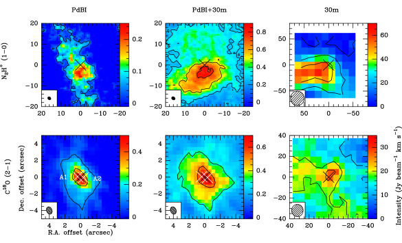
Figure 1: Integrated intensity maps of N₂H⁺ (1$-$0) (top) and C¹⁸O (2$-$1) (bottom) emission from the PdBI (left), combined (middle), and 30m (right) datasets for L1448-2A. The white crosses represent the positions of the binary system determined from the 1.3 mm dust continuum emission. The black cross represents the middle position between the binary system. The clean beam is shown by an ellipse on the bottom left of each map. The black lines represent the integrated intensity contours of each tracer starting at 5$\sigma$ and increasing in steps of 25$\sigma$ for N₂H⁺ and 10$\sigma$ for C¹⁸O (see Tables 9 and 10). Be careful, the spatial scales of the maps are not uniform in all panels.

4 Envelope kinematics from high dynamic range datasets

4.1 Integrated intensity maps

To identify at which scales of the protostellar envelopes the different datasets are sensitive to, we produced integrated intensity maps by integrating spectra of each pixel for the molecular lines C¹⁸O (2$-$1) and N₂H⁺ (1$-$0) from the PdBI, combined, and 30m datasets for each source. For C¹⁸O (2$-$1), we integrated each spectrum on a velocity range of $\pm$ 2.5 km s^-1 around the velocity of the peak of the mean spectrum of each source. The 1$-$0 line of N₂H⁺ has a hyperfine structure with seven components (see Fig. 2). We integrated the N₂H⁺ spectra over a range of 20 km s^-1 encompassing the seven components. Figure 1 shows as an example the integrated intensity maps obtained for L1448-2A. The integrated intensity maps of the other sources are provided in Appendix H.

We used the integrated intensity maps to measure the average emission size of each tracer in each dataset above a 5$\sigma$ threshold. The values reported in Tables 9 and 10 are the average of two measurements: an intensity cut along the equatorial axis and circular averages at different radii around the intensity peak position of the source. Only pixels whose intensity is at least 5 times higher than the noise in the map are considered to build these intensity profiles. The FWHM of the adjustment by a Gaussian function allows us to determine the average emission size of the sources. For both tracers and for all sources in our sample, the emission is detected above 5$\sigma$ in an area larger in the combined datasets than in the PdBI datasets, and smaller than in the 30m ones (see Tables 9 and 10). Our three datasets are thus not sensitive to the same scales and allow us to probe different scales within the 12 sampled protostellar envelopes: the 30m datasets trace the outer envelope, the PdBI datasets the inner part and the combined ones the intermediate scales.

The C¹⁸O and N₂H⁺ molecules do not trace the same regions of the protostellar envelope either: Anderl et al. (2016) report from an analysis of the CALYPSO survey that the N₂H⁺ emission forms a ring around the central C18O emission in four sources. Previous studies (Bergin et al., 2002; Maret et al., 2002, 2007; Anderl et al., 2016) show that N₂H⁺, which is abundant in the outer envelope, is chemically destroyed when the temperature in the envelope reaches the critical temperature ($T\gtrsim$20K) at which CO desorbs from dust ice mantles. Thus, while N₂H⁺ can be used to probe the envelope kinematics at outer envelope scales, C¹⁸O can be used as a complementary tracer of the gas kinematics at smaller radii where the embedded protostellar embryo heats the gas to higher temperatures.

The C¹⁸O emission is robustly detected ($>$5$\sigma$) in our PdBI observations for most sources, except for L1521F and IRAM04191 which are the lowest luminosity sources of our sample (see Table 2), and for SVS13-B where the emission is dominated by its companion, the Class I protostar SVS13-A. For most sources, the interferometric map obtained with the PdBI shows mostly compact emission ($r<3\hbox{${}^{\prime\prime}$}$, see Table 9). However, the C¹⁸O emission from the 30m datasets shows more complex structures (see Appendix H). Assuming that, under the hypothesis of spherical geometry, the emission from a protostellar envelope is compact ($r\lesssim$40^′′, i.e., $\lesssim$10000 au, see Table 2) and stands out from the environment in which it is embedded, the 30m emission of L1448-2A, L1448-C, and IRAS4A comes mainly from the envelope.

The N₂H⁺ emission is detected in our combined observations for all sources. In the four sources studied by Anderl et al. (2016), they do not detect the emission at the 1.3 mm continuum peak, but emission rings around the C¹⁸O central emission. From Table 10, we noticed two types of emission morphologies based on the PdBI dataset: compact ($r<$7^′′, see Table 10) or filamentary ($r\geq$9^′′). In the same way as the C¹⁸O emission, the N₂H⁺ emission from the 30m datasets shows complex structures with radius $r\gtrsim$40^′′ for most sources, except for five sources (IRAM04191, L1521F, L1448-NB, L1448-C, and L1157) where the emission is consistent with the compact emission of the protostellar envelope.

The C¹⁸O emission from the PdBI is not centered on the continuum peak for three sources in our sample: IRAS4A, L1448-NB, and L1448-2A (see Appendix H). For each of these sources, the PdBI 1.3 mm dust continuum emission map resolves a close binary system ($<$600 au) with both components embedded in the same protostellar envelope (Maury et al. 2019, see Table 2). The origin of the coordinate offsets is chosen to be the main protostar, secondary protostar, and the middle of the binary system for IRAS4A, L1448-NB, and L1448-2A, respectively, to study the kinematics in a symmetrical way.

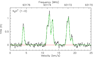
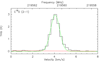
Figure 2: Mean spectra of the N₂H⁺ (top) and C¹⁸O (bottom) molecular lines from the 30m datasets for L1448-2A. The best fits of the spectra, by a hyperfine structure and a Gaussian line profile models respectively, are represented in green solid lines. In the top panel, the velocity axis corresponds to the isolated HFS component $1_{01}-0_{12}$. The systemic velocity is estimated to be 4.10 km s^-1 for this source (see Table 14).

4.2 Velocity gradients in protostellar envelopes

To quantify centroid velocity variations at all scales of the protostellar envelopes, we produced centroid velocity maps of each Class 0 protostellar envelope by fitting all individual spectra (pixel by pixel) by line profile models in the CLASS program of the GILDAS software. We only considered the line intensity detected with a signal-to-noise ratio higher than 5. We fit the spectra to be able to deal with multiple velocity components. Indeed, because protostellar envelopes are embedded in large-scale clouds, multiple velocity components can be expected on some lines of sight where both the protostellar envelope and the cloud emit. For example, Belloche et al. (2006) find several velocity components in their 30m of the N₂H⁺ emission of IRAS4A (see Appendix H.6). Except for IRAS4A and IRAS4B for which we fit two velocity components (see details in Appendix H), for most sources we used a Gaussian line profile to model the C¹⁸O (2$-$1) emission, with the line intensity, full width at half maximum (FWHM), and centroid velocity let as free parameters (see Fig. 2). In the case of N₂H⁺ (1$-$0), we used a hyperfine structure (HFS) line profile to determine the FWHM and centroid velocity of the molecular line emission (see Fig. 2). Figures 3 to 14 show the centroid velocity maps obtained for each source of the sample using the PdBI, combined, and 30m datasets for both the C¹⁸O and N₂H⁺ emission.

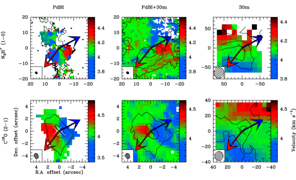
Figure 3: Centroid velocity maps of N₂H⁺ (1$-$0) (top) and C¹⁸O (2$-$1) (bottom) emission from the PdBI (left), combined (middle), and 30m (right) datasets for L1448-2A. The blue and red solid arrows represent the directions of the blue- and red-shifted outflow lobes, respectively. The white crosses represent the positions of the binary system determined from the 1.3 mm dust continuum emission (see Table 2). The black cross represents the middle position between the binary system. The clean beam is shown by an ellipse on the bottom left. The integrated intensity contours in black are the same as in Fig. 1.

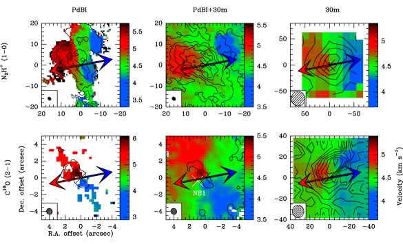
Figure 4: Same as Figure 3, but for L1448-NB. The white cross represents the position of main protostar L1448-NB1 determined from the 1.3 mm dust continuum emission (see Table 2). The black cross represents the position of the secondary protostar L1448-NB2 of the multiple system.

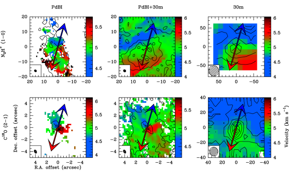
Figure 5: Same as Figure 3, but for L1448-C.

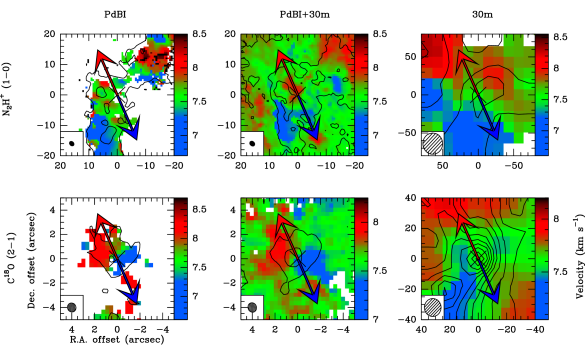
Figure 6: Same as Figure 3, but for IRAS2A.

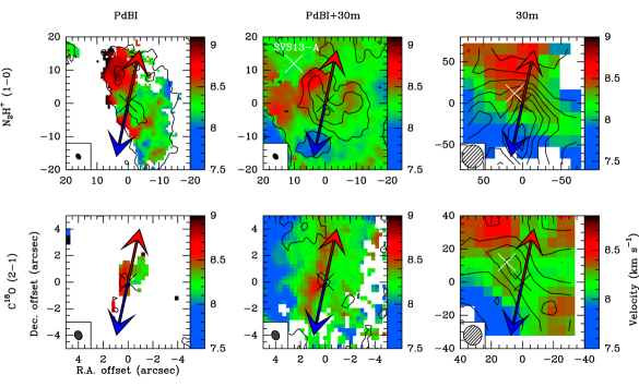
Figure 7: Same as Figure 3, but for SVS13-B. The white cross represents the position of the Class I protostar SVS13-A determined from the 1.3 mm dust continuum emission (Maury et al., 2019).

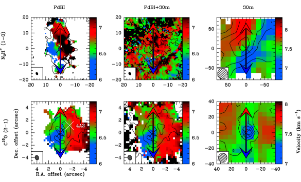
Figure 8: Same as Figure 3, but for IRAS4A. The white cross represents the position of secondary protostar IRAS4A2 determined from the 1.3 mm dust continuum emission (see Table 2). The black cross represents the position of the main protostar IRAS4A1 of the multiple system.

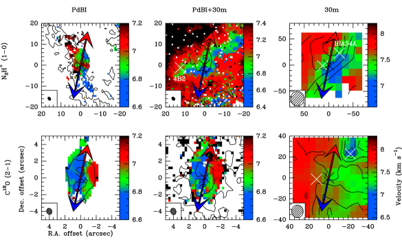
Figure 9: Same as Figure 3, but for IRAS4B. The white crosses represent the position of secondary protostar IRAS4B2 and the position of IRAS4A, respectively, determined from the 1.3 mm dust continuum emission (see Table 2). The black cross represents the position of the secondary protostar L1448-NB2 of the multiple system.

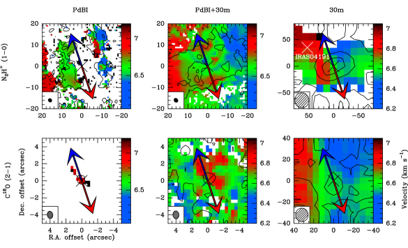
Figure 10: Same as Figure 3, but for IRAM04191. The white cross represents the position of the Class I protostar IRAS04191. The black cross represents the position of IRAM04191 determined from the 1.3 mm dust continuum emission (see Table 2).

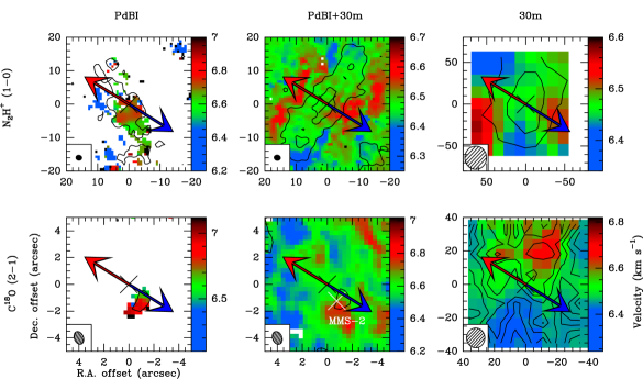
Figure 11: Same as Figure 3 for L1521F. The white cross represents the position of the starless dense core MMS-2.

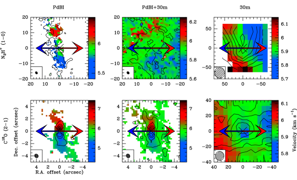
Figure 12: Same as Figure 3, but for L1527.

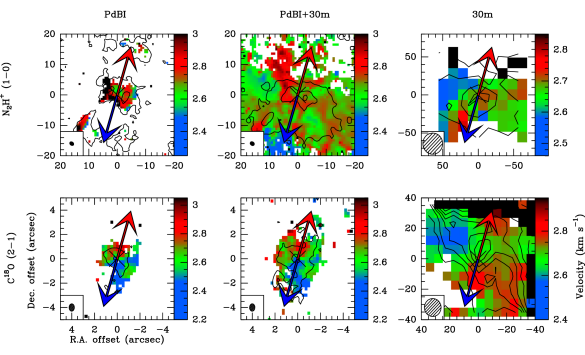
Figure 13: Same as Figure 3, but for L1157.

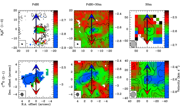
Figure 14: Same as Figure 3, but for GF9-2.

For most sources in our sample, these centroid velocity maps reveal organized velocity patterns with blue-shifted and red-shifted velocity components on both sides of the central stellar embryo, along the equatorial axis where such velocity gradients could be due to rotation of the envelopes. The global kinematics in Class 0 envelopes is a complex combination of rotation, infall, and outflow motions. The observed velocities are projected on the line of sight and thus, are a mix of the various gas motions. Therefore, it is not straightforward to interpret a velocity gradient in terms of the underlying physical process producing it. In order to have an indication of the origin of these gradients, we performed a least-square minimization of a linear velocity gradient model on the velocity maps following:

$$\rm{v}_{\mathrm{grad}}=\rm{v}_{0}+a\Delta\alpha+b\Delta\beta,$$ (1)

with $\Delta\alpha$ and $\Delta\beta$ the offsets with respect to the central source (Goodman et al., 1993).

This simple model provides an estimate of the reference velocity $\mathrm{v}_{0}$ called systemic velocity, the direction $\Theta$, and the amplitude $G$ of the mean velocity gradient. One would expect a mean gradient perpendicular to the outflow axis if the velocity gradient was due to rotational motions in an axisymmetric envelope. A mean gradient oriented along the outflow axis could be due to jets and outflows or infall in a flattened geometry. The gradients were fit on the region of the velocity maps shown in Fig. 3, namely 10$\hbox{${}^{\prime\prime}$}\times$ 10^′′ in the PdBI and combined datasets for the C¹⁸O emission (lower left and central panels), 40$\hbox{${}^{\prime\prime}$}\times$ 40^′′ for the N₂H⁺ emission from the PdBI and combined datasets (upper left and central panels), and 80$\hbox{${}^{\prime\prime}$}\times$ 80^′′ and 160$\hbox{${}^{\prime\prime}$}\times$ 160^′′, respectively for the C¹⁸O and N₂H⁺ emission from the 30m datasets (right panels). Table 2 reports for each source the significant mean velocity gradients detected with an amplitude higher than 2$\sigma$. No significant velocity gradient is observed for IRAM04191, L1521F, and SVS13-B in C¹⁸O emission at scales of $r<$5^′′or for L1448-C and IRAS4B at $r>$30^′′(see Table 2).

Seven of the 12 sources in our sample show a mean gradient in C¹⁸O emission aligned with the equatorial axis ($\Delta\Theta<$30^∘) which could trace rotational motions of the envelope at scales of $r<$5^′′. At similar scales, four sources (L1448-NB, L1521F, L1157, GF9-2) show gradients with intermediate orientation (30${}^{\circ}<\Delta\Theta<$60^∘). Finally, L1448-2A shows a mean gradient aligned to the outflow axis rather than the equatorial axis ($\Delta\Theta>$60^∘). For these last five sources, the gradients observed could be due to a combination of rotation, ejection, and infall motions. For all sources, we noticed a systematic dispersion of the direction of the velocity gradient from inner to outer scales in the envelope (see Fig. 19). We discuss in Sect. 5.4 whether this shift in direction of the velocity gradient is due to a transition from rotation-dominated inner envelope to collapse-dominated outer envelope at $r>$1500 au, or is due to the different molecular tracers used for this analysis. In most sources, the gradient moves away from the equatorial axis as the scale increases. Only three sources (IRAM04191, L1521F, and L1527) show a gradient close to the equatorial axis with $\Delta\Theta<$30^∘ at 2000 au in N₂H⁺ emission from the combined dataset while four sources show a complex gradient and five sources have a $\Delta\Theta>$60^∘.

Table 2: Estimation of the systemic velocity, the mean velocity gradient amplitude and its orientation from linear gradient fit of centroid velocity maps in C¹⁸O and N₂H⁺ emission from the PdBI, the combined, and the 30m datasets for the CALYPSO sample sources.

Source

Line

PdBI

PdBI+30m

30m

$G$

v0

$\Theta$

$\Delta\Theta$

$G$

v0

$\Theta$

$\Delta\Theta$

$G$

v0

$\Theta$

$\Delta\Theta$

(km s-1 pc-1)

(km s-1)

(∘)

(∘)

(km s-1 pc-1)

(km s-1)

(∘)

(∘)

(km s-1 pc-1)

(km s-1)

(∘)

(∘)

L1448-2A

C18O (2-1)

118 $\pm$ 3

4.06 $\pm$ 0.03

107 $\pm$ 2

69

13 $\pm$ 2

4.05 $\pm$ 0.04

81 $\pm$ 1

43

6 $\pm$ 1

4.12 $\pm$ 0.02

-14 $\pm$ 2

52

N2H+ (1-0)

19 $\pm$ 1

4.09 $\pm$ 0.03

-89 $\pm$ 2

53

2 $\pm$ 1

4.10 $\pm$ 0.04

-177 $\pm$ 21

35

2 $\pm$ 1

4.16 $\pm$ 0.04

-8 $\pm$ 3

46

L1448-NB

C18O (2-1)

214 $\pm$ 1

4.71 $\pm$ 0.06

51 $\pm$ 1

41

75 $\pm$ 1

4.55 $\pm$ 0.05

50 $\pm$ 1

40

6 $\pm$ 1

4.45 $\pm$ 0.02

85 $\pm$ 4

75

N2H+ (1-0)

108 $\pm$ 1

4.55 $\pm$ 0.02

74 $\pm$ 1

64

13 $\pm$ 1

4.57 $\pm$ 0.02

100 $\pm$ 1

90

4 $\pm$ 1

4.51 $\pm$ 0.01

97 $\pm$ 1

87

L1448-C

C18O (2-1)

218 $\pm$ 4

5.13 $\pm$ 0.05

-119 $\pm$ 2

12

62 $\pm$ 1

5.03 $\pm$ 0.05

-138 $\pm$ 1

31

–

–

–

–

N2H+ (1-0)

15 $\pm$ 2

4.92 $\pm$ 0.03

-175 $\pm$ 4

68

13 $\pm$ 1

4.97 $\pm$ 0.03

-179 $\pm$ 1

72

7 $\pm$ 1

4.85 $\pm$ 0.01

-152 $\pm$ 1

45

IRAS2A

C18O (2-1)

150 $\pm$ 5

7.75 $\pm$ 0.08

101 $\pm$ 2

14

17 $\pm$ 1

7.63 $\pm$ 0.06

97 $\pm$ 3

18

3 $\pm$ 1

7.66 $\pm$ 0.01

-10 $\pm$ 1

55

N2H+ (1-0)

11 $\pm$ 1

7.57 $\pm$ 0.04

-20 $\pm$ 6

45

4 $\pm$ 1

7.64 $\pm$ 0.03

20 $\pm$ 4

85

5 $\pm$ 1

7.61 $\pm$ 0.01

-5 $\pm$ 1

60

SVS13-B

C18O (2-1)

–

–

–

–

28 $\pm$ 4

8.19 $\pm$ 0.08

89 $\pm$ 10

12

7 $\pm$ 1

8.15 $\pm$ 0.02

-33 $\pm$ 1

70

N2H+ (1-0)

16 $\pm$ 1

8.48 $\pm$ 0.03

74 $\pm$ 1

3

5 $\pm$ 1

8.31 $\pm$ 0.02

16 $\pm$ 4

61

7 $\pm$ 1

8.07 $\pm$ 0.02

-4 $\pm$ 1

81

IRAS4A

C18O (2-1)

105 $\pm$ 1

6.57 $\pm$ 0.04

-79 $\pm$ 1

11

18 $\pm$ 4

6.72 $\pm$ 0.06

-80 $\pm$ 17

10

1.2 $\pm$ 0.4

7.57 $\pm$ 0.04

8 $\pm$ 13

82

N2H+ (1-0)

43 $\pm$ 1

6.85 $\pm$ 0.05

-69 $\pm$ 1

21

7 $\pm$ 1

6.90 $\pm$ 0.06

37 $\pm$ 2

53

3 $\pm$ 1

7.48 $\pm$ 0.02

51 $\pm$ 1

39

IRAS4B

C18O (2-1)

65 $\pm$ 1

6.84 $\pm$ 0.03

-89 $\pm$ 1

14

52 $\pm$ 5

6.89 $\pm$ 0.06

-83 $\pm$ 8

20

–

–

–

–

N2H+ (1-0)

25 $\pm$ 2

6.94 $\pm$ 0.04

96 $\pm$ 6

19

3 $\pm$ 1

7.06 $\pm$ 0.05

-71 $\pm$ 14

32

3 $\pm$ 1

7.47 $\pm$ 0.02

51 $\pm$ 5

27

IRAM04191

C18O (2-1)

–

–

–

–

25 $\pm$ 2

6.62 $\pm$ 0.07

-42 $\pm$ 5

28

6 $\pm$ 1

6.59 $\pm$ 0.01

96 $\pm$ 1

14

N2H+ (1-0)

11 $\pm$ 2

6.76 $\pm$ 0.05

109 $\pm$ 3

1

15 $\pm$ 1

6.64 $\pm$ 0.03

92 $\pm$ 1

18

3 $\pm$ 1

6.61 $\pm$ 0.01

124 $\pm$ 1

14

L1521F

C18O (2-1)

–

–

–

–

16 $\pm$ 1

6.57 $\pm$ 0.04

-82 $\pm$ 2

52

2 $\pm$ 1

6.49 $\pm$ 0.01

-8 $\pm$ 1

22

N2H+ (1-0)

26 $\pm$ 2

6.67 $\pm$ 0.04

-76 $\pm$ 5

46

0.7 $\pm$ 0.1

6.48 $\pm$ 0.01

-49 $\pm$ 2

19

0.4 $\pm$ 0.1

6.47 $\pm$ 0.01

6 $\pm$ 2

36

L1527

C18O (2-1)

171 $\pm$ 5

5.91 $\pm$ 0.06

-9 $\pm$ 3

9

66 $\pm$ 1

5.84 $\pm$ 0.06

22 $\pm$ 2

22

2 $\pm$ 1

5.94 $\pm$ 0.01

113 $\pm$ 1

67

N2H+ (1-0)

17 $\pm$ 1

5.87 $\pm$ 0.03

9 $\pm$ 6

9

3 $\pm$ 1

5.91 $\pm$ 0.02

26 $\pm$ 5

26

2 $\pm$ 1

5.91 $\pm$ 0.01

123 $\pm$ 4

57

L1157

C18O (2-1)

104 $\pm$ 3

2.61 $\pm$ 0.06

13 $\pm$ 2

60

68 $\pm$ 2

2.63 $\pm$ 0.06

35 $\pm$ 2

38

2 $\pm$ 1

2.70 $\pm$ 0.15

-125 $\pm$ 8

18

N2H+ (1-0)

51 $\pm$ 2

2.82 $\pm$ 0.04

35 $\pm$ 2

38

0.8 $\pm$ 0.4

2.69 $\pm$ 0.02

113 $\pm$ 65

40

1.0 $\pm$ 0.5

2.65 $\pm$ 0.04

-131 $\pm$ 35

24

GF9-2

C18O (2-1)

126 $\pm$ 17

-3.01 $\pm$ 0.06

-154 $\pm$ 4

64

17 $\pm$ 1

-2.83 $\pm$ 0.03

-133 $\pm$ 5

43

2 $\pm$ 1

-2.62 $\pm$ 0.01

102 $\pm$ 1

12

N2H+ (1-0)

18 $\pm$ 3

-2.80 $\pm$ 0.01

-123 $\pm$ 8

33

1.4 $\pm$ 0.1

-2.56 $\pm$ 0.01

-9 $\pm$ 5

81

0.5 $\pm$ 0.1

-2.56 $\pm$ 0.01

40 $\pm$ 8

50

4.3 High dynamic range position-velocity diagrams to probe rotational motions

To investigate rotational motions and characterize the angular momentum properties in our sample of Class 0 protostellar envelopes, we build the position-velocity (PV_rot) diagrams along the equatorial axis. We assumed the position angle of the equatorial axis as orthogonal to the jet axis reported in Table 2. The choice of this equatorial axis allows us to maximize sensitivity to rotational motions and minimize potential contamination on the line of sight due to collapsing or outflowing gas (Yen et al., 2013). The velocities reported in the PV_rot diagram are corrected for the inclination $i$ of the equatorial plane with respect to the line of sight (see Table 2). We note that the correction for inclination is a multiplicative factor, thus if this inclination angle is not correctly estimated, the global observed shape is not distorted.

The analysis described in detail in Appendix C allows us to build a PV_rot diagram with a high dynamic range from 50 au up to 5000 au for each source as follows (see the example of L1527 in Fig. 15):
$\bullet$ To constrain the PV_rot diagram at the smallest scales resolved by our dataset ($\sim$0.5^′′), we use the PdBI C¹⁸O datasets that we analyze in the (u,v) plane to avoid imaging and deconvolution processes (see label ”C¹⁸O PdBI” in Fig. 15). We only kept central emission positions in the channel maps at a position angle $<$—45${}^{\circ}|$ with respect to the equatorial axis (see Appendix C).
$\bullet$ Since the C¹⁸O extended emission is filtered out by the interferometer, we used the combined C¹⁸O emission to populate the PV_rot diagram at the intermediate scales of the protostellar envelopes (see label ”C¹⁸O combined” in Fig. 15). The C¹⁸O molecule remains the most precise tracer when the temperature is higher than $\sim$20K because below, the C¹⁸O molecule freezes onto dust ice mantles. To determine the transition radius $R_{\mathrm{trans}}$ between the two tracers, we calculate the C¹⁸O and N₂H⁺ column densities along the equatorial axis from the combined integrated intensity maps (see Appendix D and green points in Fig. 15).
$\bullet$ At radii $r>R_{\mathrm{trans}}$, the N₂H⁺ emission traces better the envelope dense gas. We use the combined N₂H⁺ emission maps to analyze the envelope kinematics at larger intermediate scales. When the N₂H⁺ column density profile reaches a minimum value due to the sensitivity of the combined dataset, this dataset is no longer the better dataset to provide a robust information on the velocity (see label ”N₂H⁺ combined” in Fig. 15).
$\bullet$ Finally, we use the 30m N₂H⁺ emission map to populate the PV_rot diagram at the largest scales of the envelope (see label ”N₂H⁺ 30m” in Fig. 15).

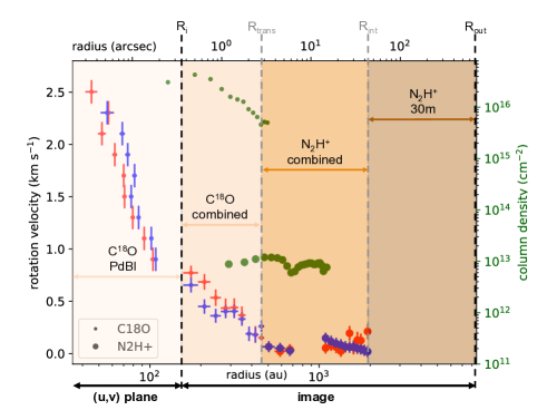
Figure 15: Plot summarizing the combination of tracers and datasets used to build high dynamic range PV_rot diagrams in the L1527 envelope. The transition radii between the different datasets (PdBI, combined, and 30m) and the two C¹⁸O and N₂H⁺ tracers represented by the dashed lines are given in Table 11. The green points show the column density profiles along the equatorial axis of C¹⁸O and N₂H⁺ estimated from the combined datasets (see Appendix D).

The CALYPSO datasets allow us to continuously estimate the velocity variations along the equatorial axis in the envelope over scales from 50 au up to 5000 au homogeneously for each protostar. Figure 16 shows the PV_rot diagrams built for all sources of the sample. The systemic velocity used in the PV_rot diagrams are determined in Appendix E.

The method of building PV_rot diagrams described above and in Appendix C corresponds to an ideal case with a detection of a continuous blue-red velocity gradient along the direction perpendicular to the outflow axis in the velocity maps. In practice, the direction of velocity gradients is not always continuous at all scales probed by our observations (see Table 2 and Figure 19). For some sources, to constrain the PV_rot diagrams, we did not take the kinematic information at all scales of the envelope into account. Velocity gradients can be considered as probing rotational motions if the following criteria are met:
$\indent\bullet$ We only consider the significant velocity gradients reported in Table 2 with a blue- and a red-shifted velocity components observed on each side of the protostellar embryo, itself at the systemic velocity $\mathrm{v}_{0}$. For example, we only take the C¹⁸O emission from the 30m map into account for L1521F (see Fig. 11).
$\indent\bullet$ We only take the velocity gradients aligned with the equatorial axis ($\Delta\Theta<$60^∘) into account in order to minimize contamination by infall and ejection motions. For example, we do not report in the PV_rot diagrams the N₂H⁺ velocity gradients from the combined maps for L1448-NB, IRAS2A, SVS13-B, and GF9-2 (see Table 2).
$\indent\bullet$ We do not consider the discontinuous velocity gradients which show an inversion of the blue- and red-shifted velocity components along the equatorial axis from inner to outer envelope scales. For example, we do not report in the PV_rot diagrams the N₂H⁺ velocity gradients from the 30m maps for IRAM04191 and L1157 (see Figs. 10 and 13).

When velocity gradients with a blue- and a red-shifted velocity components observed on each side of the protostellar embryo are continuous from inner to outer envelope scales but shifted from the equatorial axis ($\Delta\Theta\geq$60^∘), we only report upper limits on rotational velocities in the PV_rot diagrams. The sources in our sample show specific individual behaviors, therefore we followed as closely as possible the method of building the PV_rot diagram adapting it on a case-by-case basis.

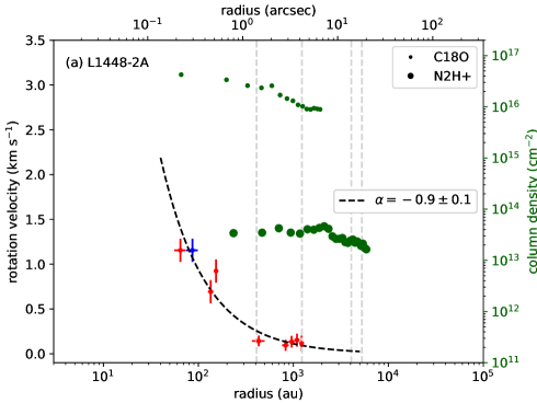
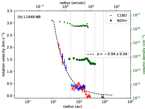
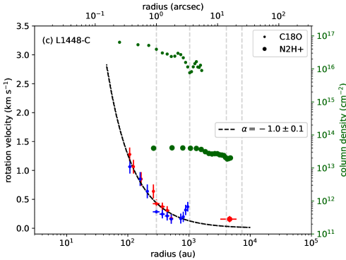
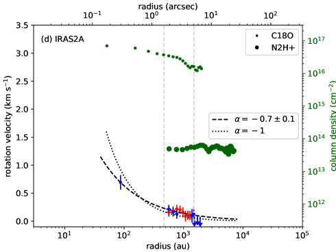
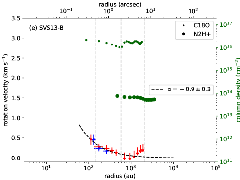
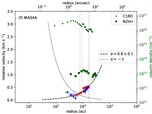
Figure 16: Position-velocity diagram along the equatorial axis of the CALYPSO protostellar envelopes. Blue and red dots show the blue- and red-shifted velocities, respectively. The arrows display the upper limits of $\mathrm{v}_{\mathrm{rot}}$ determined from velocity maps that do not exhibit a spatial distribution of velocities as organized as one would expect from rotation motions (see Sect. 4.3 and Appendix C). Green dots show the column density profiles along the equatorial axis. Dots and large dots show the C¹⁸O and N₂H⁺ data, respectively. The dashed curve shows the best fit with a power-law model leaving the index $\alpha$ as a free parameter ($\mathrm{v}_{\mathrm{rot}}\propto r^{\alpha}$) whereas the dotted curve shows the best fit with a power-law model with a fixed index $\alpha$=-1. The vertical dashed lines show the transition radii between the different datasets (PdBI, combined, and 30m) and the two tracers as illustrated in Fig. 15 and given in Table 11.

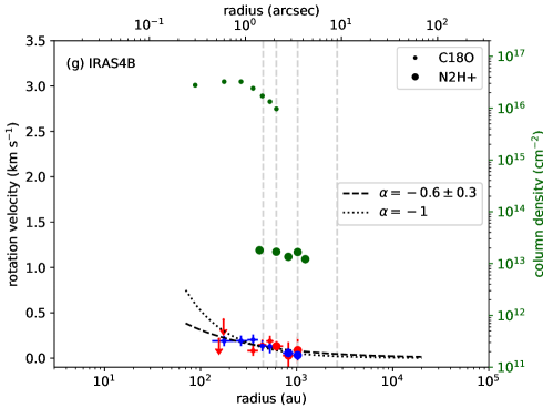
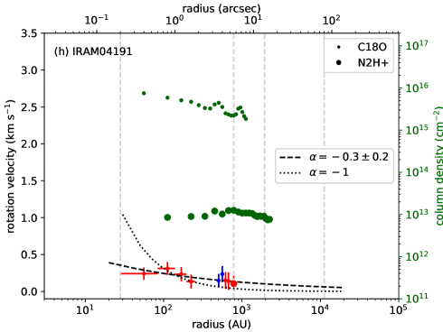
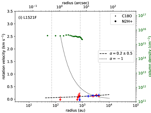
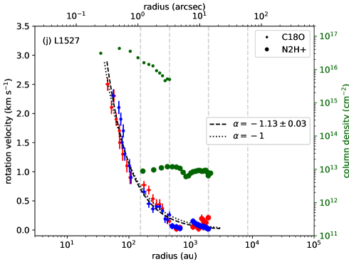
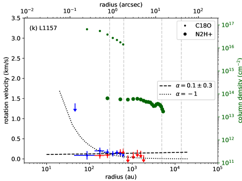
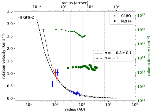
Figure 16: Continued.

5 Discussion

In this section, we discuss the presence of rotation in the protostellar envelopes from the PV_rot diagrams (see Sect. 5.1 and Fig. 16). We build the distribution of specific angular momentum associated with the PV_rot diagrams (see Sect. 5.2) and explore the possible solutions to explain the $j(r)$ profiles observed in the inner ($r<$1600 au, see Sect. 5.3) and outer ($r>$1600 au, see Sect. 5.4) parts of the envelopes.

5.1 Characterization of rotational motions

We assume that the protostellar envelopes are axisymmetric around their rotation axes, and thus, the velocity gradients observed along the equatorial axis, and reported in the PV_rot diagrams, are mostly due to the rotational motions of the envelopes. We model the rotational velocity variations by a simple power-law model $\mathrm{v}\propto r^{\alpha}$ without taking the upper limits into account. This method has been tested with an axisymmetric model of collapsing-rotating envelopes by Yen et al. (2013). As long as rotation dominates the velocity field on the line of sight, which depends on the inclination and flattening of the envelope, Yen et al. (2013) obtain robust estimates of the rotation motions at work in the envelopes. First, we fix the power-law index at $\alpha$=-1 to compare to what is theoretically expected for an infalling and rotating envelope from a progenitor core in solid-body rotation (Ulrich, 1976; Cassen & Moosman, 1981; Terebey et al., 1984; Basu, 1998). The reduced $\chi^{2}$ values of fits by an orthogonal least-square model are reported in the second column of Table 3. Then, we let the power-law index vary as a free parameter: the best power-law index and the reduced $\chi^{2}$ found for each protostellar envelope in our sample are reported in the third column of Table 3. Figure 16 shows the PV_rot diagrams adjusted by a power-law for the sources of the CALYPSO sample.

Table 3: Parameters of best power-law fits to the PV_rot diagrams.

Source	Radial range	Power law fit $\alpha$=-1		Power law fit
		DoF	$\chi^{2}$	DoF	$\alpha$	$\chi^{2}$
	(au)
L1448-2A	60$-$1250	8	1.3	7	-0.9 $\pm$0.1	1.4
L1448-NB	150$-$1700	34	2.3	33	-0.94 $\pm$0.04	2.3
	150$-$350	…	…	5	-0.9 $\pm$0.2	0.4
L1448-C	100$-$4000	19	1.6	18	-1.0 $\pm$0.1	1.7
IRAS2A	85$-$1500	13	0.9	12	-0.7 $\pm$0.1	0.2
SVS13-B	110$-$450	7	0.2	6	-0.9 $\pm$0.3	0.2
IRAS4A	250$-$1600	18	20.4	17	0.8$\pm$0.1	1.5
	250$-$550	…	…	5	-1.3$\pm$0.6	0.6
IRAS4B	175$-$1050	12	0.6	11	-0.6 $\pm$0.3	0.5
IRAM04191	55$-$800	9	1.1	8	-0.3 $\pm$0.2	0.3
L1521F	1500$-$4200	6	1.0	5	0.2 $\pm$0.5	0.1
L1527	45$-$2000	58	1.9	57	-1.13 $\pm$ 0.03	1.6
L1157	85$-$650	10	1.2	9	0.1 $\pm$0.3	0.3
GF9-2	75$-$850	10	2.0	9	-0.8 $\pm$0.1	1.8

The power-law indices of the PV_rot diagrams from our sample are between -1.1 and 0.8. Five sources (L1448-2A, IRAS2A, SVS13-B, L1527, and GF9-2) show rotational velocity variations in the envelope scaling as a power law with an index close to -1. This is consistent with the expected index for collapsing and rotating protostellar envelopes. The reduced $\chi^{2}$ are $\sim$1.5 for these sources except for IRAS2A and SVS13-B for which it is better ($\sim$0.2). L1521F and L1157 show a power-law index close to 0 with a very low reduced $\chi^{2}$ ($\leq$0.3, see Table 3). These flat PV_rot diagrams ($\mathrm{v}_{\mathrm{rot}}\sim$ constant) suggest differential rotation of the envelope with an angular velocity of $\Omega=\frac{v_{\mathrm{rot}}}{r}\propto r^{-1}$. For two other sources (IRAS4B and IRAM04191), the best indices are compatible with -0.5, which could suggest Keplerian rotation at scales of $r<$1000 au. However, the reduced $\chi^{2}$ are also satisfactory ($\sim$1) when we fix the power-law index at $\alpha$=-1 (see Table 3). Thus, for these two sources, our CALYPSO datasets only allow us to estimate a range of the power-law indices between -1 and -0.5 (see Table 3).

Rotational velocity variations along the equatorial axis between 50 and 5000 au in L1448-NB cannot be reproduced satisfactorily by any single power-law model ($\chi^{2}>$2, see Table 3). However, considering only the points at $r<$400 au for L1448-NB, we obtain a power-law index of -0.9$\pm$0.2 with a good reduced $\chi^{2}$ of 0.4, as expected for a collapsing and rotating envelope (see Table 3).

We found a positive index $\alpha$ for IRAS4A of 0.8 (see Table 3). It could be an indication of solid-body rotation of $\Omega=\frac{v_{\mathrm{rot}}}{r}\sim$constant. However, we observe that the velocity in the PV_rot diagram decreases from 2000 to $\sim$600 au and re-increases at small scales (see panel (f) of Fig. 16). Thus, the velocity gradient is not uniform on the scales traced by the PV_rot diagram as would be expected for a solid-body rotation ($\mathrm{v}_{\mathrm{rot}}\propto r$). Moreover, points at radii $<$600 au are consistent with an infalling and rotating envelope (see panel (f) of Fig. 16): considering only these points, we obtain a power-law index of -1.3$\pm$0.6 with a good reduced $\chi^{2}$ value of 0.6 (see Table 3). There is a dip in the C¹⁸O emission at $r<$350 au that could be due to the opacity (see Figures 41 and 40), thus, below this radius the information on velocities could be altered. To date, no observations have identified any solid-body rotating protostellar envelope. Numerical models also favor differential rotation of the envelope (Basu, 1998). The interpretation of the velocity field as tracing solid-body rotation in the envelope of IRAS4A is therefore unlikely to be correct.

For the sources IRAS2A, IRAM04191, and L1157, the reduced $\chi^{2}$ is also good ($\sim$1) when the PV_rot diagrams of these sources are ajusted by a model with a fixed index of $\alpha$=-1 (see Table 3). We determine position and velocity from four different and independent methods and we did not consider the uncertainties of the connection between the different tracers and datasets. The uncertainty on the indices reported in Table 3 may thus be underestimated. On the other hand, although we determined the systemic velocity by maximizing the overlap of the blue and red points, this method does not allow a more accurate determination than 0.05 km s^-1. The systematic error of 0.05 km s^-1, added to previous velocity errors of the points in the PV_rot diagrams to take this uncertainty on the systemic velocity into account (see Appendix E), can be overestimated and thus lead us to underestimate the $\chi^{2}$. For these three sources, the CALYPSO dataset only allow us to estimate a range of power-law indices between -1 and the $\alpha$ value reported in the fifth column of Table 3. The uncertainties on the indices reported in Table E are statistical errors and a systematic uncertainty of $\pm$0.1 has to be added to account for the uncertainties in the outflow directions and thus the equatorial axis directions (see Table 2). Moreover, despite the choice of the equatorial axis, the rotational velocities could be contaminated by infall at the small scales along this axis due to the envelope geometry.

To conclude, the organized motions reported in the PV_rot diagrams and modeled by a power-law function with an index $\alpha$ ranging from -2 to 0 are consistent with differential rotational motions ($\Omega\propto r^{\epsilon}$, with -3$<\epsilon<$-1 here). We identified rotational motions in all protostellar envelopes in our sample except in IRAS4A.

5.2 Distribution of specific angular momentum in the CALYPSO Class 0 envelopes

5.2.1 Specific angular momentum due to rotation motions

Assuming the motions detected along the equatorial axis are dominated by differential rotation for 11 of the 12 sources in our sample, we use the measurements reported in the PV_rot diagrams to derive the radial distribution of specific angular momentum in the protostellar envelopes due to rotation. In this part of the study, IRAS4A is excluded. The specific angular momentum is $j=\frac{J}{M}=\frac{I\Omega}{M}$ with the moment of inertia $I$ defined as $I\propto Mr^{2}$ (Belloche, 2013). Thus, the specific angular momentum is calculated from the rotational velocity: $j=\mathrm{v}_{\mathrm{rot}}(r)\times r$. We plot all the specific angular momentum profiles obtained for the CALYPSO subsample in panel (b) of Fig. 17. The individual distribution of specific angular momentum $j(r)$ for each source is given in Appendix H. This is the first time that the specific angular momentum distribution as a function of radius within a protostellar envelope is determined homogeneously for a large sample of 11 Class 0 protostars. We performed a least-square fit of the $j(r)$ profiles for each source individually, using a model of a simple power-law and a broken power-law model to identify the change of regimes. The broken power-law model function is defined with a break radius $r_{\mathrm{break}}$ as follows:

$$j(r)\propto\left(\frac{r}{r_{\mathrm{break}}}\right)^{\beta_{1}}\leavevmode\nobreak\ \leavevmode\nobreak\ \mathrm{when}\leavevmode\nobreak\ \leavevmode\nobreak\ r<r_{\mathrm{break}},$$

$$j(r)\propto\left(\frac{r}{r_{\mathrm{break}}}\right)^{\beta_{2}}\leavevmode\nobreak\ \leavevmode\nobreak\ \mathrm{when}\leavevmode\nobreak\ \leavevmode\nobreak\ r>r_{\mathrm{break}}.$$

We report in Table 16 the power-law indices fitting the best individual profiles and the associated reduced $\chi^{2}$. For the broken power-law fits, only results with a reduced $\chi^{2}$ better than the one obtained with a simple power-law model and with a break radius value $r_{\mathrm{break}}$ to which the $j(r)$ profile is really sensitive, have been retained.

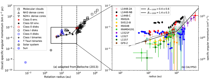
Figure 17: Radial distribution of specific angular momentum. Panel (a): Figure adapted from Figure 8 of Belloche (2013) and from Ohashi et al. (1997b). Panel (b): zoom on the region where the angular momentum profiles due to rotation of the CALYPSO sources lie. The gray curve shows the median profile $j(r)$. In the two panels, the solid black line shows the best fit with a broken power-law model.

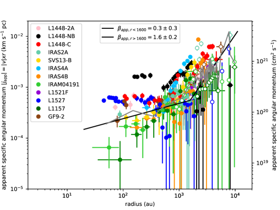
Figure 18: Radial distribution of apparent specific angular momentum $|j_{\mathrm{app}}|=|v|\times r$ along the equatorial axis of the CALYPSO sources, considering all the velocity gradients observed at all envelope scales, including the reversed gradients and the shifted ones at scales of $r\gtrsim$1600 au (see Fig. 19 and Sect. 5.4) which were excluded in the construction of the PV_rot diagrams in Fig. 16, and in panel (b) of Fig. 17 for our analysis of rotational motions. The empty circles show the negative apparent specific angular momentum from the reversed gradients along the equatorial axis in the outer scales ($r>$1600 au) of the L1448-2A, IRAS2A, IRAM04191, L1527, L1157 and GF9-2 envelopes (see Sect. 5.4.1). The gray curve shows the median profile —$j_{\mathrm{app}}$— and the solid black line shows the best fit with a broken power-law model.

Two sources (L1448-NB and L1448-C) are better reproduced by a broken power-law model than a simple power-law model where the $\chi^{2}$ are $\sim$2: this allows us to identify a change of slope from a relatively flat profile to an increasing profile at larger radius in the envelope ($\beta\sim$1), with break radii between 500 and 700 au. For the other sources, we also identified at scales of $r<$1300 au a flat profile of specific angular momentum with $\beta<0.5$ (L1448-2A, IRAS2A, SVS13-B, IRAS4B, L1527, and GF9-2) while the specific angular momentum profile at scales of $r>$1000 au shows a steeper slope with $\beta\sim$1 (L1521-F). However, two sources of the sample (IRAM04191 and L1157) stand out as the sources showing a steep increase in their specific angular momentum profile at scales of $r<$1000 au ($\beta\geq$0.7), similar to the indices found at large radii in the sources showing a break in their $j(r)$ profiles. We note that for the flat profiles ($\beta<$0.5; L1448-2A, SVS13-B, IRAS4B, and GF9-2), and IRAM04191 and L1157, the specific angular momentum distribution is only constrained at scales $<$1300 au. Most of the sources in our sample are better reproduced by a broken power-law model with a break radius (1000 $\pm$ 500) au and an increasing profile at larger radius in the envelope ($\beta\sim$1.4) than a simple power-law model.

In his review, Belloche (2013) plotted the observed specific angular momentum as a function of rotation radius for several objects along the star-forming sequence. In this plot (panel (a) of Figure 17), he identifies three regimes in the distribution of specific angular momentum, that can be broadly associated with different evolutionary stages:
$\bullet$ prestellar regime: on large scales, the apparent angular momentum of molecular clouds (Goldsmith & Arquilla, 1985) and dense cores (Goodman et al., 1993; Caselli et al., 2002) appears to follow the power-law relation $j\propto r^{1.6}$,
$\bullet$ protostellar regime: between 100 au and $\sim$6000 au (0.03 pc), a few points in different protostellar envelopes suggest the specific angular momentum is relatively constant ($j\sim 10^{-3}$ km s^-1 pc, Ohashi et al. 1997b; Belloche et al. 2002; Chen et al. 2007),
$\bullet$ disk and binary regime: below 100 au, measurements in disks and Class II binaries (Chen et al., 2007) show a decrease of $j$ following a trend characteristic of Keplerian rotation ($j\propto r^{0.5}$).

Thus, from previous observational studies on rotational motions, finding a break at $r\sim$1000 au between two trends of specific angular momentum within Class 0 protostars was unexpected. Although the velocity gradients observed in the outer part of the protostellar envelopes ($r>$1000 au) are consistent with rotational motions, the observed $j$ regime at these scales is not expected from pure rotational motions.

5.2.2 Apparent specific angular momentum

The radius range of $j(r)$ distribution due to rotation motions is not homogeneous between sources (see Table 16). To identify whether the radius of $\sim$1000 au is a critical radius between two trends of specific angular momentum in each source, we derive the radial distribution of the apparent specific angular momentum —$j_{\mathrm{app}}$— at all scales in the envelopes. To build —$j_{\mathrm{app}}$—$(r)$ distribution, we consider the gradients observed at all envelope scales, including also the reversed gradients and the shifted ones at scales of $r\gtrsim$1000 au (see Fig. 19 and Sect. 5.4) which were excluded in the construction of the PV_rot diagrams in Fig. 16 because they are not consistent with rotational motions. By considering these velocity gradients, we add points in the outer envelopes but the trend observed in the inner envelopes do not change (see Tables 16 and 17). Thus, the —$j_{\mathrm{app}}$—$(r)$ distribution helps us to understand the origin of the trend and the velocity gradients observed at $r>$1000 au. We plot all the apparent specific angular momentum profiles obtained for the CALYPSO subsample in Fig. 18. We also report the apparent specific angular momentum of IRAS4A which was identified as the only source that did not show any rotational motions in our sample (see Sect. 5.1). As for $j$ profiles, we performed a least-square fit of the —$j_{\mathrm{app}}$—$(r)$ profiles for each source individually and we report the indices of the power-law models in Table 17.

We create the median —$j_{\mathrm{app}}$—$(r)$ profile of the CALYPSO subsample. We first resampled the individual profile of each source in steps of 100 au and normalized it by the value at 600 au, then we took the median value of individual profiles at each radius step. The median profile is shown in gray on Figure 18. From a broken power-law fit, we obtain a relatively flat profile ($j_{\mathrm{app}}\propto r^{0.3\pm 0.3}$) at radii smaller than 1570$\pm$300 au and an increasing profile ($j_{\mathrm{app}}\propto r^{1.6\pm 0.2}$) in the outer envelope. The radius of $\sim$1600 au therefore appears to be a critical radius which delimits two regimes of angular momentum in protostellar envelopes: the specific angular momentum decreases down to $\sim$1600 au and then tends to become constant.

The change of behavior of $j_{\mathrm{app}}$ above the break radius could be due to a change of tracer to study the kinematics in the outer envelope. However, we do not find any systematic consistency between $r_{\mathrm{app,break}}$ and the transition radius $R_{\mathrm{trans}}$ between the two tracers C¹⁸O and N₂H⁺. Even if for SVS13-B, $R_{\mathrm{trans}}$ is in the error bars of $r_{\mathrm{app,break}}$, for three sources (L1448-NB, L1448-C, and IRAS4A) it is not consistent, and for IRAS4B, we do not observe a change of regime for $j_{\mathrm{app}}$ at $r\sim$1600 au (see Tables 16 and 17). Moreover, for L1521F, only the C¹⁸O emission shows a velocity gradient allowing us to constrain the kinematics at scales of $r>$1600 au (see Fig. 11) and we find the same trend of $j_{app}$ ($\beta_{\mathrm{app}}\sim$1.2) than in all other sources where we used N₂H⁺ to constrain the outer part of the envelopes. The other sources (L1448-2A, IRAS2A, IRAM04191, L1527, L1157, and GF9-2) show a negative value of the apparent angular momentum at outer envelope scales due to a renversal of the velocity gradients (see Fig. 18, Table 17, and Sect. 5.4.1). For two of these sources (L1448-2A and GF9-2) the radius where the gradient reverses along the equatorial axis, resulting in a negative $j_{\mathrm{app}}$ with respect to the inner envelope scales, is consistent with $R_{\mathrm{trans}}$ and $r_{\mathrm{app,break}}$. For two sources (IRAS2A and IRAM04191), $R_{\mathrm{trans}}$ is consistent with the radius where the gradient reverses along the equatorial axis but not with $r_{\mathrm{app,break}}$. For the last two sources (L1527 and L1157), the three radii are all different from each other. The different individual behaviors in the CALYPSO sample allow us to conclude that our finding that protostellar envelopes are characterized by two regimes of angular momentum does not result from our use of two different tracers.

From the median —$j_{\mathrm{app}}$—$(r)$ profile without normalization of the individual profiles at 600 au, we find a mean value of specific angular momentum in the inner parts of the envelopes ($r<$1600 au) of $\sim$6 $\times$10^-4 km s^-1 pc. This value is slightly lower but compatible with the estimates made by Ohashi et al. (1997b) and Chen et al. (2007) in four Class 0 or I sources ($j\sim$10^-3 km s^-1 pc at $r<$5000 au). It is also consistent with the studies by Yen et al. (2015a) and Yen et al. (2015b) which find values between 5 $\times$ 10^-3 km s^-1 pc and 5 $\times$ 10^-5 km s^-1 pc in the inner envelope (r$<$1500 au). Yen et al. (2015a) estimate a specific angular momentum of $\sim 5\times$ 10^-4 km s^-1 pc at $r\sim$100 au for L1448-C and L1527. Moreover, our values for L1157 are consistent with their upper limit estimate of $5\times$ 10^-5 km s^-1 pc in the inner envelope ($r<$100 au) of L1157.

The high angular resolution and the high dynamic range of the CALYPSO observations allow us to identify the first two regimes within individual protostellar envelopes: values at radii $\gtrsim$1600 au ($j_{\mathrm{app}}\propto r^{1.6}$ on average, see Table 17) seem to correspond to the trend found in dense cores at scales $>$6000 au while the values stabilize around $\sim$6 $\times$10^-4 km s^-1 pc on average at radii $<$1600 au. This study resolves for the first time the break radius between these two regimes deeper within the protostellar envelopes at around $\sim$1600 au instead of $\sim$6000 au. In a study of ammonia emission in the outer envelopes of two Class 0 objects, Pineda et al. (2019) find an increasing angular momentum profile scaling as $r^{1.8}$ from 1000 au to 10000 au, with values $\sim$3 $\times$10^-4 km s^-1 pc at radii $\sim$1000 au. They do not detect the break around $\sim$1600 au found in the CALYPSO sample. This break radius from which the profiles are found to be flat in the inner envelope may depend on the evolutionary stage of the accretion process during the Class 0 phase as suggested by Yen et al. (2015b). It could be due to the propagation of the inside-out expansion wave during the collapse (Shu, 1977): assuming a median lifetime or half life of $\sim$5 $\times$10⁴ yr for Class 0 protostar envelopes (Maury et al. 2011; see also Evans et al. 2009) at sound velocity ($\sim$ 0.2 km s^-1), one obtains a radius $\sim$2000 au. This radius is on the same order of magnitude as the observed break radius between the two regimes observed in the distribution of specific angular momentum of sources in our sample. In this case, the break radius could be an indication of the age of the protostars, except for four sources (L1448-NB, IRAM04191, L1521F, and L1157) in our sample where we do not observe this break radius. Beyond this radius, the outer envelope may not have collapsed yet, and could therefore retain the initial conditions in angular momentum of the progenitor prestellar core.

This could be an explanation for the increase in angular momentum observed at the scales of $r>$1600 au ($j_{\mathrm{app}}\propto r^{1.6}$ on average, see Table 17), consistent with the prestellar stage ($j\propto r^{1.6}$). We discuss the properties and physical origin of these two regimes in more details in the next sections.

5.3 Conservation of angular momentum in Class 0 inner envelopes

In this section, we focus on the relatively constant values of specific angular momentum observed in the inner envelopes at scales of $r\leq$1600 au in the $j(r)$ profiles due to rotation motions (see Fig. 17). From these flat profiles, we find that the matter directly involved in the formation of the stellar embryo has a specific angular momentum $\sim$3 orders of magnitude higher than the one in T-Tauri stars ($j\sim$2 $\times$10^-7 km s^-1 pc, Bouvier et al. 1993). We discuss constant values of specific angular momentum as conservation of angular momentum to test disk formation as a possible solution to the angular momentum problem.

It is difficult to constrain the time evolution of specific angular momentum for a given particle from angular momentum distributions which are snapshots of the angular momentum distribution of all particles at a given time during the collapse phase. During the collapse of a core initially in either solid-body rotation or differential rotation, particles conserve their specific angular momentum during the accretion on the stellar embryo (Cassen & Moosman, 1981; Terebey et al., 1984; Goodwin et al., 2004). In the case of a protostellar envelope with a density profile $\rho\propto r^{-2}$, an observed flat profile $j(r)=$constant requires, since each particle at different radii has the same specific angular momentum, an initially uniform distribution of angular momentum. This does not agree with the steep increase in specific angular momentum we observe at scales of $r>$1600 au in the $j(r)$ profiles. The break in the specific angular momentum profile could be due either to a faster collapse of the inner envelope caused by an initial inner density plateau (Takahashi et al., 2016) or to a change of dominant mechanisms responsible for the observed velocity gradients from inner to outer scales of the envelope.

In our sample, we distinguish eight sources with a relatively flat $j(r)$ profile in the inner envelope ($\beta<$0.5, see Table 16): L1448-2A, L1448-NB, L1448-C, IRAS2A, SVS13-B, IRAS4B, L1527, and GF9-2. We estimate a centrifugal radius that would be obtained when the mass currently observed at $\sim$100 au collapses and based on the mean value of specific angular momentum observed today $<j_{\mathrm{100\leavevmode\nobreak\ au}}>$ as follows:

$$R_{\mathrm{cent}}=\frac{<j_{\mathrm{100\leavevmode\nobreak\ au}}>^{2}}{G\leavevmode\nobreak\ M_{\mathrm{100\leavevmode\nobreak\ au}}}.$$ (2)

The lower limit of the mass enclosed within 100 au, $M_{\mathrm{100\leavevmode\nobreak\ au}}$, is the mass of the envelope $M_{\mathrm{100\leavevmode\nobreak\ au}}^{\mathrm{dust}}$ estimated from the PdBI 1.3 mm dust continuum flux (Maury et al., 2019), assuming optically thin emission, a dust temperature at 100 au computed with Eq. (4) and corrected by the assumed distance (see Table 2). This mass estimate does not include the mass of the central stellar object, $M_{\star}$: since the embryo mass is unknown for most sources in our sample, we consider an upper limit of $M_{\mathrm{100\leavevmode\nobreak\ au}}=M_{\star}+M_{\mathrm{100\leavevmode\nobreak\ au}}^{\mathrm{dust}}$ assuming $M_{\star}=$ 0.2 M_⊙ for each source in our sample. This value of 0.2 M_⊙ corresponds to the stellar mass in the Class 0/I protostar L1527 from kinematic models of the Keplerian pattern in the disk (Tobin et al., 2012; Ohashi et al., 2014; Aso et al., 2017). The range of values for $M_{\mathrm{100\leavevmode\nobreak\ au}}$ are reported in the third column in Table 4. The calculated range of centrifugal radii associated with $M_{\mathrm{100\leavevmode\nobreak\ au}}$ is listed for each source in the fourth column in Table 4. We note that if $M_{\star}$ of a source is smaller than that of L1527, then the centrifugal radius value we calculated is underestimated.

Since the embryo mass is uncertain and $M_{\mathrm{100\leavevmode\nobreak\ au}}$ may be underestimated if the dust emission is not optically thin, we compute the mass enclosed within $r<$100 au, including the stellar embryo mass, needed to form a disk the size of $R_{\mathrm{disk}}^{\mathrm{dust}}$ with the $<j_{\mathrm{100\leavevmode\nobreak\ au}}>$ observed. The values are reported in the last column of Table 4.

Table 4: Centrifugal radius $R_{\mathrm{cent}}$ assuming angular momentum conservation.

Source	$<j_{\mathrm{100\leavevmode\nobreak\ au}}>$	$M_{\mathrm{100\leavevmode\nobreak\ au}}$	$R_{\mathrm{cent}}$	$R_{\mathrm{disk}}^{\mathrm{dust}}$	$M_{100\leavevmode\nobreak\ au}^{\mathrm{min}}$
	(10-4 km s-1 pc)	($M_{\odot}$)	(au)	(au)	($M_{\odot}$)
L1448-2A	4.5$\pm$0.2	0.005 $-$ 0.2	50$-$1810	$<$50	0.2
L1448-NB	16.0$\pm$0.4	0.042 $-$ 0.2	500$-$2920	$<$50	3.0
L1448-C	6.0$\pm$0.2	0.025 $-$ 0.2	70$-$690	41$\pm$15	0.5
IRAS2A	3.8$\pm$0.4	0.020 $-$ 0.2	30$-$330	$\lesssim$65	0.1
SVS13-B	2.5$\pm$0.2	0.019 $-$ 0.2	10$-$160	$\lesssim$75	0.05
IRAS4B	2.5$\pm$0.3	0.003 $-$ 0.2	10$-$840	155$\pm$30	0.02
L1527	5.6$\pm$0.1	0.001 $-$ 0.2	70$-$1060	54$\pm$10	0.3
GF9-2	3.9$\pm$0.3	0.002 $-$ 0.2	40$-$3080	36$\pm$9	0.2

For all the sources in our sample, the upper limits of the $R_{\mathrm{cent}}$ range are larger than 150 au and systematically larger than the continuum disk candidate radii $R_{\mathrm{disk}}^{\mathrm{dust}}$ from Maury et al. (2019) reported in the fifth column of Table 4. Moreover, Maret et al. (2020) only detect possible Keplerian rotation in two protostars in our sample (L1527 at radii $\sim$90 au and L1448-C at $r\sim$200 au) from the CALYPSO data. Thus, most $R_{\mathrm{cent}}$ values is expected to be less than 100 au. The upper $R_{\mathrm{cent}}$ values are probably overestimated because the contribution of the embryo mass to $M_{\mathrm{100\leavevmode\nobreak\ au}}$ is excluded.

Comparing the lower limits of the $R_{\mathrm{cent}}$ range with the candidate disk radius, we find a good agreement for most sources in our sample except for L1448-NB. We find a larger centrifugal radius ($\sim$500 au) than the observed disk size ($<$50 au) calculated considering only the main protostar L1448-NB1 of the binary system. Since in this study, we are interested in the kinematics of the whole system, we must consider all the continuum structure and not only that of the main protostar. Considering NB1 and NB2, Maury et al. (2019) resolve a circumbinary structure with a radius of (320 $\pm$ 90) au centered on the middle of the two components. Given the uncertainties, the latter value is consistent with the lower centrifugal radius estimated here. At these scales, Tobin et al. (2016a) observe a spiral structure surrounding the multiple system and interpreted it as a gravitationally unstable circumbinary disk. On the other hand, Maury et al. (2019) suggest that this component is due to orbital motions and tidal arms between the companions and Maret et al. (2020) do not detect any Keplerian rotation at radii $<$170 au. Thus, the nature of this additional structure surrounding the multiple system is still unclear. As a consequence, the increase in specific angular momentum we measured at small scales could not only trace the rotation of the disk or the envelope but may be contaminated by gravitational instabilities due to orbital motions or a fragmented disk surrounding the system. Given the large uncertainties on the dust disk radii, we found a good agreement between centrifugal radii and $R_{\mathrm{disk}}^{\mathrm{dust}}$ for L1448-C and L1527. Moreover, the dust radius (50 au in L1527, Maury et al. 2019) does not necessarily exactly correspond to the centrifugal radius which was first detected in L1527 from observations of SO emission at 100$\pm$20 au (Sakai et al., 2014). For this source, our estimate of $R_{\mathrm{cent}}$ ($\sim$70 au) is consistent with previous kinematic studies which detect a proto-planetary disk candidate with a radius of 50$-$90 au (Ohashi et al., 2014; Aso et al., 2017; Maret et al., 2020). Moreover, we observe a slight increase in the specific angular momentum we measured at $r<$80 au. It could be due to the transition from the envelope to the disk.

The hypothesis of collapsing material with conservation of angular momentum, resulting in disk formation, at $r<$100 au is therefore plausible for most sources in our sample. We notice that L1448-NB, in which Tobin et al. (2016a) claim the detection of a large candidate disk, shows the highest value of specific angular momentum at $r<$1600 au of the CALYPSO sample, consistent with the angular momentum observed in the proto-planetary disks surrounding the T-Tauri stars which are estimated to be 1$-$6$\times$10^-3 km s^-1 pc (Simon et al., 2000; Kurtovic et al., 2018; Pérez et al., 2018). It could suggest an increase in the angular momentum of the disk during its evolution. In this case, the mean value of $j(r)$ in the inner envelope would be lower in the less evolved than in the more evolved Class 0 protostars, and it would increase with time until reaching the value contained in the T-Tauri disks. In this scenario, L1448-NB would be one of the most evolved objects in the sample. However, the borderline Class 0/I protostar L1527, which is the most evolved object of the CALYPSO sample, has a specific angular momentum of $\sim$6 $\times$ 10^-4 km s^-1 pc at the inner envelope scales (see Table 4). In the same way, L1448-C has a specific angular momentum less than one order of magnitude lower than the values observed in the Class II disks while Maret et al. (2020) suggest the presence of a Keplerian disk in the inner envelope. As most of the CALYPSO inner protostellar envelopes have an order of magnitude less specific angular momentum than in Class II disks, we discuss below several possible explanations:
(i) a part of the angular momentum inherited by the T-Tauri disks may not come from the rotating matter contained in the inner envelope accreted during the Class 0 phase. During the Class I phase, the mass accreted could come from regions further away from the envelope ($r\gg$1600 au) with a possibly higher specific angular momentum.
(ii) disks may expand with time due to the transfer of angular momentum from their inner regions to their outer ones. Unfortunately, the specific angular momentum does not contain information about the mass. Large values of $j(r)$ may be carried by low masses at the outer disk radius but may remain difficult to quantify. To this day, the mechanisms at work in disk evolution remain an open question. Some studies, for example, suggest that viscous friction may be responsible for the disk expansion (Najita & Bergin, 2018).
(iii) the specific angular momentum of the proto-planetary disks may be biased toward high values from historical, large and massive disks. A new population of small T-Tauri disks with radii between 10 and 30 au has been observed thanks to PdBI and ALMA (Piétu et al., 2014; Cieza et al., 2019). Assuming a small rotationally-supported disks around a stellar object including a total mass of 0.1$-$1 $M_{\odot}$ (Piétu et al., 2014), one expects a specific angular momentum between 10^-5 km s^-1 pc and 10^-4 km s^-1 pc, values which are similar to those we obtained in the inner Class 0 protostellar envelopes with the CALYPSO sample. However, to this day, no resolved observations of gas kinemactics of these small Class II disks allow us to estimate observationally their specific angular momentum.

5.4 Origin of the velocity gradients at $r>$1600 au

At outer envelope scales, we detect velocity gradients ($\sim$2 km s^-1 pc^-1 at $\sim$10000 au, see Table 2) in the CALYPSO single-dish maps. They may not be directly related to rotational motions of the envelopes but rather to other mechanisms. Indeed, we observe in the CALYPSO dataset a systematic evolution of the orientation of the gradients between the inner and outer scales in the envelope (see Table 2). Figure 19 shows the orientation of the mean velocity gradient observed at different scales of the envelope with respect to the position angle of the gradient observed at scales $\sim$100 au. The clear dispersion ($\sim$100^∘ on average, see Fig. 19) of gradient position angle across scales within individual objects may be due to a change of dominant mechanisms responsible for the observed gradients from inner to outer scales of the envelope. From the literature, velocity gradients are often measured in the outer protostellar envelopes along the equatorial axis and they are interpreted as due to rotational motions or infall from a filamentary structure at scales of 1500$-$10000 au (Ohashi et al., 1997b; Belloche et al., 2002; Tobin et al., 2011). In this section, we explore the possible origins of the velocity gradients found at scales of $r>1600$ au and used to build the —$j_{\mathrm{app}}$—$(r)$ profiles (see Fig. 18).

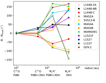
Figure 19: Evolution of the orientation of the mean velocity gradient in the different datasets used to build the PV_rot diagrams and angular momentum distributions with respect to the PA of the velocity gradient observed at small scales $\Theta_{\mathrm{small}}$ (PdBI C¹⁸O emission). The error bars of the orientation $\Theta$ are given in Table 2. They are smaller than $10^{\circ}$ except for 7 of the 67 gradient measurements. For these 7 measurements, the large error bars are generally due to the absence of a clear gradient on either side of the central position of the source. Gradient measurements with large error are indicated by an empty circle. A typical error of $\pm 10^{\circ}$ is shown on the first point of the plot.

5.4.1 Questioning the interpretation of counter-rotation

Six sources in the sample show a clear reversal of the orientation of the mean velocity gradient ($|\Theta-\Theta_{\mathrm{small}}|>130^{\circ}$) from the inner to the outer envelope scales: IRAS4A, IRAS4B, L1527, IRAM04191, L1157, and GF9-2. We note that the kinematics at scales where we observed reversed velocity gradients ($r>$1600 au) with respect to the small scales were not taken into account to build the PV_rot diagrams in Fig. 16, or the specific angular momentum profiles shown for the full sample in panel (b) of Fig. 17. Indeed, these profiles were aimed at characterizing the rotational motions in the envelopes and the angular momentum due to this rotation: a reversal of the rotation, if real, would require a more complex model than the power-law ($\mathrm{v}\propto r^{\alpha}$) model we adopted in Sects. 4.3 to 5.3. In this section, we discuss these complex patterns in more detail.

In IRAM04191, we observed velocity gradients at outer envelope scales of $r>$1600 au consistent with those observed previously by Belloche et al. (2002) and Lee et al. (2005) ($\Theta\sim$100^∘, see Table 2). However, in the inner envelope, we noticed a velocity gradient with a direction of $\Theta=$-83^∘ (see bottom middle panel in Fig. 10 and Table 2). In L1527, we found small-scale velocity gradients ($\Theta\sim$0^∘ at $r\sim$ 1000 au) consistent with those previously observed by Tobin et al. (2011) which are in the opposite direction compared to the large-scale one ($r\sim$8000 au, Goodman et al. 1993). Tobin et al. (2011) interpret this reversal of velocity gradients as counter-rotation but it also could be due to infalling motions that dominated the velocity field at the outer envelope scales (Harsono et al., 2014).

Our study suggests that reversals of velocity gradients are common in Class 0 protostellar envelopes. However, the asymmetrical velocity gradients (for IRAS4B, GF9-2), the filamentary structures traced by the integrated intensity at scales of $r>$2000 au (for IRAS4A, IRAS4B, L1527, and GF9-2), and a strong external compression of the cloud hosting IRAS4A and IRAS4B (Belloche et al., 2006) lead us to exclude the observed reversed gradients as counter-rotation of the envelope. Moreover, only MHD models with Hall effect succeed to form envelopes in counter-rotation. These models form a thin layer of counter-rotating envelopes at the outer radius of the disk ($r\sim$50-200 au; Tsukamoto et al. 2017). This envelope layer is in counter-rotation compared to the formed disk and the protostellar envelope at $r>$200 au as a consequence of the Hall effect generated by the rotation of the disk which changes the angular momentum of the gas at the disk outer radius. Therefore, these models cannot explain the inversions of rotation in the different layers of the envelope at scales of $r>$3000 au as observed in our sample. Historically, the gradients observed from single-dish mapping at $r>$3000 au have been used to quantify the amplitude for the angular momentum problem. However, incorrectly interpreted as pure rotational motions in the envelope, the resulting angular momentum measurements and the expected disk radii would be significantly overestimated.

Recent studies on the angular momentum of the protostellar cores from hydrodynamical simulations of star formation are questioning the standard model of star formation from a collapsing core initially in solid-body rotation (Kuznetsova et al., 2019; Verliat et al., 2020). They show that the angular momentum of synthetic protostellar cores is not directly related to the initial rotation of the synthetic cloud, and Keplerian disks can be formed from a simple non-uniform perturbation in the initial density distribution. In this scenario, the angular momentum observed in inner protostellar envelopes and disks may not been inherited from larger-scale initial conditions but generated during the collapse itself.

5.4.2 Contribution of infalling motions and core-forming motions

The misalignments between the gradients observed in the envelopes at inner and outer envelope scales suggest a change of dominant mechanisms at $r>$1600 au. At large scales, infalling motions of the envelope can dominate rotational motions. In the hypothesis of a flattened infalling envelope, infall motions are expected to produce a velocity gradient projected in the plane of the sky that is oriented along the minor axis of the envelope, namely at the same position angle as the outflow. In L1448-NB, SVS13-B and L1527, we detect velocity gradients aligned with the outflow axis at $r>$3000 au while at small scales the gradients are consistent with the equatorial axis (see Table 2). These three sources could be good candidates of the transition from collapse to rotation between large and small scales. This scenario is also suggested in the study of Ohashi et al. (1997a). They suggested that at outer envelope scales of $r\sim$2000 au, the protostellar envelope L1527 is not rotationally supported ($\mathrm{v}_{\mathrm{rot}}\sim$0.05 km s^-1) but is dominated by the collapse ($\mathrm{v}_{\mathrm{inf}}\sim$0.3 km s^-1).

Currently, there are very few constraints on the infall velocities at scales of $r>$1600 au in the CALYPSO protostellar envelopes. Belloche et al. (2002) estimate an infall velocity of $\mathrm{v}_{\mathrm{inf}}\sim$0.15 km s^-1 at $r\sim$1000 au from radiative transfer modeling of CS and C³⁴S emission in IRAM04191. In the dense core L1544, Tafalla et al. (1998) suggest also an infall velocity of $\sim$0.1 km s^-1 at scales $>$3000 au. The velocity offset, with respect to the systemic velocity assumed for each source, found along the equatorial axis at $>$1000 au with CALYPSO is reported in Table 5. For most sources, we find typical velocity offsets $\lesssim$0.3 km s^-1 at scales of 1600 au (see Table 5), consistent with infall velocities found in IRAM04191 and L1544, except for IRAS4A. IRAS4A harbors a velocity of $\sim$0.5 km s^-1 at $r\sim$1000 au. This result is consistent with those of Belloche et al. (2006) at $\sim$2000 au. They suggest that a fast collapse is triggered by an external compression from the cloud in which the source is embedded. Thus, for all sources in our sample, the velocity gradient misalignment could be due to a change of mechanism dominating the velocities projected on the line of sight. This suggests either rotational velocities much smaller than infall velocities or a non axisymmetric geometry of the kinematics at outer envelope scales.

Moreover, Herschel observations have shown that most solar-type prestellar cores and protostars form in filaments (André et al., 2014). Indeed, the column density maps of the Herschel Gould Belt Survey program (André et al., 2010) reveal that the CALYPSO protostars are embedded in or lie in the immediate vicinity of filamentary structures with $N_{H_{2}}>$10²¹ cm^-2. Thus, the large-scale kinematics in protostellar envelopes could be contaminated or dominated by the kinematics of the filaments. Kirk et al. (2013) studied the velocity field of Serpens-South in the Aquila molecular cloud and showed a complex kinematics with longitudinal collapse along the main filament, radial contractions, and accretion streams from the cloud to the main filament. The longitudinal collapse of the filament could be responsible for the large-scale gradients observed in our protostellar envelopes as observed in the Serpens-Main region by Dhabal et al. (2018). Several studies also highlighted transverse velocity gradients perpendicular to the main filament that suggested the material may be accreting along perpendicular striations (Palmeirim et al., 2013; Dhabal et al., 2018; Arzoumanian et al., 2018; Shimajiri et al., 2019). Palmeirim et al. (2013) estimate the velocity of the infalling material to be  0.5$-$1 km s^-1 at $r\sim$0.4 pc in the B211/L1495 region. In our velocity maps at 10000 au along the equatorial axis, we measure typical velocities $<$0.3 km s^-1 in most of the sources (see Table 5) except in L1448-2A, IRAS4A, and IRAS4B. These three sources exhibit velocities of 0.5$-$1 km s^-1 consistent with infall velocities estimated at filamentary scales. In these cases, host-filament motions could dominate the kinematics in outer protostellar envelopes ($r>$1600 au).

Table 5: Value of velocity offset, with respect to the systemic velocity assumed for each source, at 100, 1000, and 10000 au along the equatorial axis from the velocity maps and considering all the gradients observed, even those not consistent with rotational motions.

Source	$\mathrm{v}_{\mathrm{100\leavevmode\nobreak\ au}}$	$\mathrm{v}_{\mathrm{1000\leavevmode\nobreak\ au}}$	$\mathrm{v}_{\mathrm{10000\leavevmode\nobreak\ au}}$
	(km s-1)	(km s-1)	(km s-1)
L1448-2A	0.7	0.1	1.1
L1448-NB	2.1	0.3	0.02
L1448-C	1.3	0.1	0.2
IRAS2A	0.7	0.1	0.3
SVS13-B	0.5	0.1	0.2
IRAS4A	…	0.4	0.9
IRAS4B	…	0.1	0.5
IRAM04191	0.3	0.1	0.1
L1521F	0.1	0.2	0.2
L1527	1.1	0.1	0.2
L1157	0.1	0.2	0.1
GF9-2	1.0	0.2	0.2

5.4.3 Contamination by turbulent motions from cloud scales

All sources of the CALYPSO subsample (except L1448-NB) reveal a steep increase in apparent specific angular momentum with the radius at $\sim$1600$-$10000 au scales, with an average trend of $j_{\mathrm{app}}\propto r^{1.6\pm 0.2}$ (see Table 17 and Fig. 18). This trend is similar to that observed in prestellar cores and clumps at scales $>$10000 au (see Figs. 17 and 18). Indeed, Goodman et al. (1993), Caselli et al. (2002) and Tatematsu et al. (2016) show a trend between the size of prestellar cores and their observed mean angular momenta at scales on the order of 0.1 pc: $j(r)$ distribution scaling as $r^{1.2-1.7}$. From this dependency of $j$ with core radius and the linewidth-size relation, Tatematsu et al. (2016) suggest that non-thermal motions (turbulence) are related to the origin of angular momentum observed in these 0.1 pc cores.

Burkert & Bodenheimer (2000) studied numerical models of turbulent molecular clouds with a symmetric density profile and a Gaussian or random velocity field. They showed that 0.1 pc cores with random motions exhibit most of the time velocity gradients that, interpreted as rotation, would have specific angular momentum values of $j\sim 3\times 10^{-3}$ km s^-1 pc (10²¹ cm² s^-1) and would scale as $j\propto r^{1.5}$. This is in good agreement with observed values at 0.1 pc from the literature (Goodman et al., 1993; Caselli et al., 2002; Tatematsu et al., 2016). Our observations showing a trend of $j\propto r^{1.6}$ at scales $\sim$1600-5000 au could be either a signature of the turbulent cascade from the large-scale ISM propagating with subsonic properties to 1600 au envelope scales, or gravitationally-driven turbulence due to large-scale collapse motions at the interface between filaments and cores (Kirk et al., 2013).

From the analysis of the gas velocity dispersion in molecular line observations, Goodman et al. (1998) and Pineda et al. (2010) identify the dense cores at a typical scale of 0.1 pc as the first velocity-coherent structures decoupled from the turbulent cloud. In this case, we would expect a quiescent structure with subsonic motions at radii $<$0.1 pc and the interpretation of ISM turbulent cascade with supersonic motions as a consequence of the steep increase of $j_{\mathrm{app}}$ at scales $<10000$ au would no longer be valid. Except L1448-2A, IRAS4A, and IRAS4B which exhibit velocities 0.5$-$1 km s^-1 consistent with supersonic turbulent motions, all sources in our sample show typical velocities $\lesssim$0.3 km s^-1 consistent with subsonic-transonic turbulent motions. This could suggest that the power-law behavior of $j_{\mathrm{app}}\propto r^{1.6}$ observed in the outer envelopes ($r>$1600 au) could be a scaling law due to the tail of a low velocity subsonic-transonic turbulent cascade.

At scales of $r>$1600 au, we observe typical velocity linewidths $\lesssim$1 km s^-1 (see Fig. 20). We note that the linewidths tend to decrease from $\sim$1600 au to larger scales in the outer envelopes and they do not show scaling laws with the radius as expected from turbulent motions in the ISM (Larson 1981; see Fig. 20 and Table 18), but the velocity structure at these scales seems to show multiple components in velocity for several sources (L1527, L1448-C, IRAS2A, SVS13-B, IRAS4A, IRAS4B). As we can not disentangle them and identify exactly which component comes from the outer envelope or the host cloud for example, we need either a more elaborate model than a Gaussian or a HFS model to analyze the spectra or a more suitable tracer to determine more robustly the linewidths of the outer envelopes.

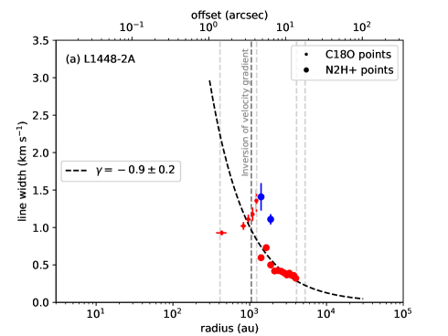
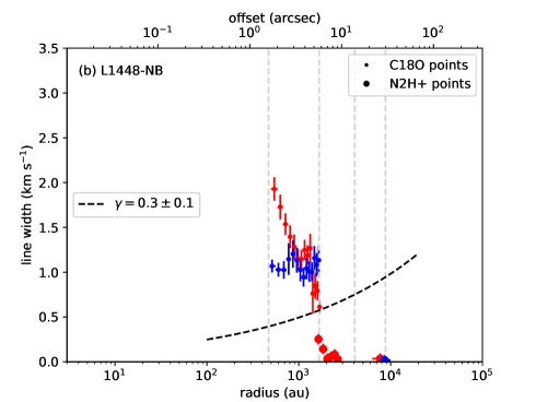
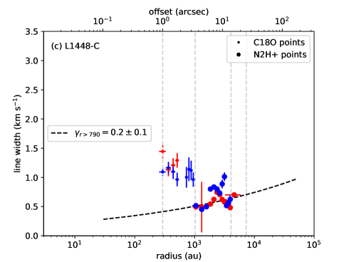
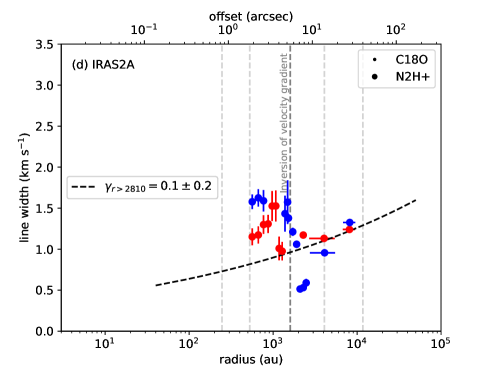
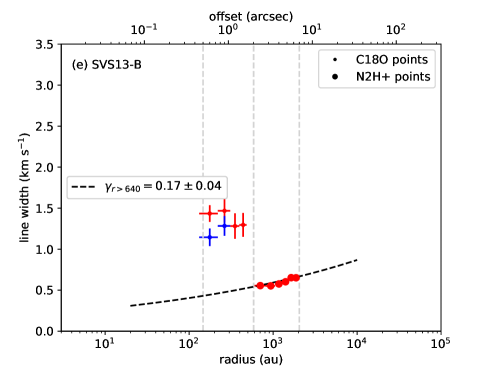
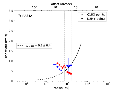
Figure 20: Linewidth along the equatorial axis of the CALYPSO protostellar envelopes. Blue and red dots show the linewidths at positions that have blue- and red-shifted velocities, respectively. Dots and large dots show the C¹⁸O and N₂H⁺ data, respectively. The dashed curve shows the best fit with a power-law model leaving the index $\gamma$ as a free parameter ($D\mathrm{v}\propto r^{\gamma}$) in the outer envelope (see Appendix G). The radius of the outer envelope is given by the break radius of the $j(r)$ or $j_{\mathrm{app}}(r)$ profiles (see Tables 16 and 17) or the radius where we observe a reversal of the velocity gradients with respect to the inner envelope. The vertical dashed lines show the transition radii between the different datasets (PdBI, combined, and 30m) and the two tracers as given in Table 11.

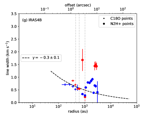
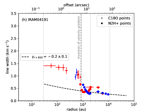
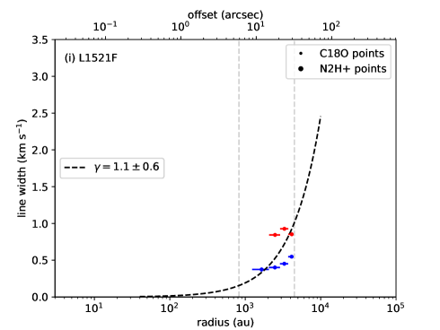
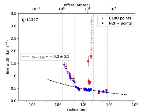
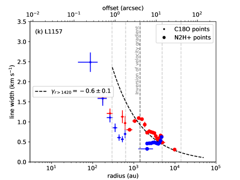
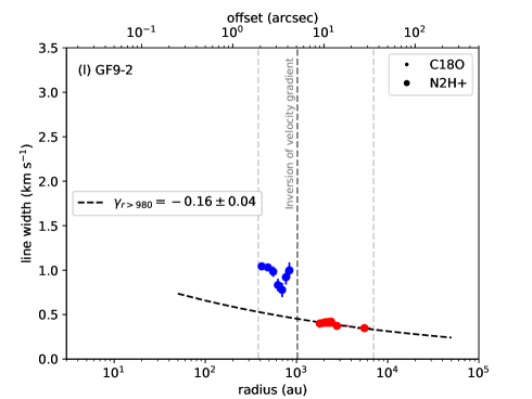
Figure 20: Continued.

6 Conclusions

In the framework of the CALYPSO survey, we analyzed the kinematics of Class 0 protostellar envelopes. The main results of our study are listed below.

1. We identify differential rotation motions in 11 sources in a sample of 12 Class 0 protostellar envelopes. The only exception is IRAS4A : the motions reported in the PV_rot and modeled by a power-law function are consistent with a solid-body rotation, but the velocity gradient is not uniform in the inner envelope at $r<$2000 au as would be expected.

2. This is the first time that the specific angular momentum distribution as a function of envelope radius is determined homogeneously for a large sample of 11 Class 0 protostars. The high angular resolution and the high dynamic range of the CALYPSO observations allow us to identify two distinct regimes: the apparent specific angular momentum decreases as $j_{\mathrm{app}}\propto r^{1.6\pm 0.2}$ down to $\sim$1600 au and then tends to become relatively constant around $\sim$6 $\times$ 10^-4 km s^-1 pc down to $\sim$50 au.

3. The values of specific angular momentum measured in the inner Class 0 envelopes suggest that material directly involved in the star formation process ($<$1600 au) typically encloses the same order of magnitude in specific angular momentum as what is inferred in small T-Tauri disks ($r\sim$10 au). The constant values of $j$ at 50$-$1600 au allow us to determine good estimates of the centrifugal radius in the Class 0 protostars of the CALYPSO sample, which compare well with the disk radii estimated from the dust continuum (Maury et al., 2019). This suggests that the specific angular momentum is conserved during the accretion on the stellar embryo, resulting in disk formation.

4. At scales of $r>$1600 au, we conclude that the velocity gradients observed in the outer envelope with respect to small scales are not due to pure rotational motions or counter-rotation motions but related to other mechanisms. Historically, the gradients observed from single-dish mapping at $r>$3000 au have been interpreted as rotation and used to quantify the amplitude of the angular momentum problem for star formation. Thus, if the gradients are incorrectly interpreted as rotation, the angular momentum problem for star formation and the expected disk radii may have been significantly over-estimated. Moreover, we find no robust hints that envelopes are rotating with typical velocities higher than the sound speed at scales of $r>$1600 au. This suggests that the origin of angular momentum in the outer protostellar envelopes could be the gravitationally-driven turbulence due to large-scale collapse motions at the interface between filaments and cores, or the dissipation of the large-scale ISM turbulent cascade propagating with subsonic velocities to 1600 au envelope scales.

Appendix A Details of IRAM 30m observations

Table 6: Details of observations carried out with the IRAM 30m telescope.

Source	Line	$\tau_{225}$	Time	Dates of observation
			(h)	(dd-month-yy)
L1448-2A	C18O (2$-$1)	0.29	1.9	04 June 2012; 16 October 2012
	N2H+ (1$-$0)	0.69	2.3	17 November 2011; 30 May 2012
L1448-NB	C18O (2$-$1)	0.28	2.3	16 November 2011; 17 November 2011; 16 October 2014
	N2H+ (1$-$0)	0.43	3.1	17 November 2011; 18 November 2011; 03 June 2012
L1448-C	C18O (2$-$1)	0.18	2.3	16 November 2011 ; 17 October 2014
	N2H+ (1$-$0)	0.41	3.1	17 November 2011; 18 November 2011; 03 June 2012
IRAS2A	C18O (2$-$1)	0.14	3.1	15 November 2011; 16 November 2011; 06 November 2014
	N2H+ (1$-$0)	0.31	1.5	15 November 2011; 17 November 2011
SVS13-B	C18O (2$-$1)	0.18	1.6	16 November 2012; 06 November 2014
	N2H+ (1$-$0)	0.64	5.4	31 May 2012; 02 June 2012; 03 June 2012; 04 June 2012
IRAS4A	C18O (2$-$1)	0.13	1.6	16 November 2012
	N2H+ (1$-$0)	0.73	3.1	01 June 2012; 04 June 2012
IRAS4B	C18O (2$-$1)	0.15	1.6	16 November 2012
	N2H+ (1$-$0)	0.62	2.7	02 June 2012
IRAM04191	C18O (2$-$1)	0.17	1.9	16 November 2011
	N2H+ (1$-$0)	0.59	3.5	17 November 2011; 18 November 2011; 02 June 2012
L1521F	C18O (2$-$1)	0.23	2.3	21 October 2014
	N2H+ (1$-$0)	0.58	5.8	18 November 2011; 30 May 2012; 03 June 2012; 04 June 2012
L1527	C18O (2$-$1)	0.18	2.3	21 October 2014; 05 November 2014; 06 November 2014; 10 November 2014
	N2H+ (1$-$0)	0.64	5.2	01 June 2012; 02 June 2012; 04 June 2012; 31 May 2015
L1157	C18O (2$-$1)	0.10	2.8	04 June 2012; 16 November 2012
	N2H+ (1$-$0)	0.60	6.1	30 May 2012; 31 May 2012; 01 June 2012
GF9-2	C18O (2$-$1)	0.09	3.1	04 June 2012; 16 November 2012; 05 November 2014
	N2H+ (1$-$0)	0.55	4.2	30 May 2012; 03 June 2012

Appendix B Properties of molecular line emission maps

Table 7: Beam sizes of the C¹⁸O (2$-$1) emission maps.

Source	PdBI	PdBI+30m	30m
	Major (′′) $\times$ Minor (′′), Pos. Ang. (∘)	Major (′′) $\times$ Minor (′′), Pos. Ang. (∘)	Major (′′) $\times$ Minor (′′), Pos. Ang. (∘)
L1448-2A	0.94 $\times$ 0.69, 24.7	0.96 $\times$ 0.70, 25.1	11.8 $\times$ 11.8, 0
L1448-NB	0.76 $\times$ 0.71, 65.5	0.77 $\times$ 0.71, 48.3	11.8 $\times$ 11.8,0
L1448-C	0.63 $\times$ 0.40, 32.0	0.63 $\times$ 0.40, 32.0	11.8 $\times$ 11.8, 0
IRAS2A	0.78 $\times$ 0.72, 49.5	0.79 $\times$ 0.72, 46.8	11.8 $\times$ 11.8, 0
SVS13-B	0.71 $\times$ 0.58, 36.5	0.73 $\times$ 0.61, 33.0	11.8 $\times$ 11.8, 0
IRAS4A	0.77 $\times$ 0.63, 31.0	0.81 $\times$ 0.67, 26.3	11.8 $\times$ 11.8, 0
IRAS4B	0.77 $\times$ 0.65, 28.9	0.82 $\times$ 0.69, 22.6	11.8 $\times$ 11.8, 0
IRAM04191	0.88 $\times$ 0.72, -166.7	0.91 $\times$ 0.75, -170.5	11.8 $\times$ 11.8, 0
L1521F	1.0 $\times$ 0.72, 26.0	1.04 $\times$ 0.75, 26.8	11.8 $\times$ 11.8, 0
L1527	0.68 $\times$ 0.58, 50.7	0.69 $\times$ 0.60, 48.9	11.8 $\times$ 11.8, 0
L1157	0.60 $\times$ 0.46, -1.3	0.61 $\times$ 0.48, -1.7	11.8 $\times$ 11.8, 0
GF9-2	0.85 $\times$ 0.75, -161.8	0.88 $\times$ 0.78, 22.0	11.8 $\times$ 11.8, 0

Table 8: Beam sizes of the N₂H⁺ (1$-$0) emission maps.

Source	PdBI	PdBI+30m	30m
	Major (′′) $\times$ Minor (′′), Pos. Ang. (∘)	Major (′′) $\times$ Minor (′′), Pos. Ang. (∘)	Major (′′) $\times$ Minor (′′), Pos. Ang. (∘)
L1448-2A	1.73 $\times$ 1.36, 64.5	1.84 $\times$ 1.46, 68.5	27.8 $\times$ 27.8, 0
L1448-NB	1.73 $\times$ 1.33, 52.4	1.88 $\times$ 1.48, 53.6	27.8 $\times$ 27.8, 0
L1448-C	1.77 $\times$ 1.40, 63.4	1.93 $\times$ 1.56, 67.0	27.8 $\times$ 27.8, 0
IRAS2A	1.72 $\times$ 1.33, 55.2	1.86 $\times$ 1.47, 55.3	27.8 $\times$ 27.8, 0
SVS13-B	1.82 $\times$ 1.29, 38.1	1.91 $\times$ 1.40, 40.4	27.8 $\times$ 27.8, 0
IRAS4A	1.83 $\times$ 1.33, 38.4	1.92 $\times$ 1.41, 42.3	27.8 $\times$ 27.8, 0
IRAS4B	1.77 $\times$ 1.27, 38.0	1.86 $\times$ 1.37, 39.7	27.8 $\times$ 27.8, 0
IRAM04191	1.84 $\times$ 1.55, 53.2	2.06 $\times$ 1.72, 52.2	27.8 $\times$ 27.8, 0
L1521F	1.83 $\times$ 1.50, 80.1	1.98 $\times$ 1.62, 81.5	27.8 $\times$ 27.8, 0
L1527	1.74 $\times$ 1.33, 45.8	1.84 $\times$ 1.45, 50.2	27.8 $\times$ 27.8, 0
L1157	1.49 $\times$ 1.10, 60.3	1.55 $\times$ 1.18, 59.6	27.8 $\times$ 27.8, 0
GF9-2	1.50 $\times$ 1.11, 68.5	1.56 $\times$ 1.16, 67.0	27.8 $\times$ 27.8, 0

Table 9: Emission size, rms noise, and integrated fluxes in the C¹⁸O (2$-$1) emission maps.

Source	PdBI			PdBI+30m			30m
	rmax	rms	Flux	rmax	rms	Flux	rmax	rms	Flux
	(′′)	(mJy beam-1)	(Jy)	(′′)	(mJy beam-1)	(Jy)	(′′)	(Jy beam-1)	(Jy)
L1448-2A	1.4	20.4	4.2	3.5	20.7	71.1	35	0.7	91.1
L1448-NB	1.6	32.9	0.7	6.9	32.6	32.6	25	0.4	191.7
L1448-C	1.0	23.5	1.1	3.0	23.4	10.4	25	0.6	95.5
IRAS2A	1.7	33.8	1.6	4.5	33.1	27.2	37	0.3	214.9
SVS13-B	0.5	20.1	5.8	7.0	19.8	35.8	42	0.9	252.3
IRAS4A	2.6	26.7	11.2	4.3	26.2	24.2	22	0.4	33.9
IRAS4B	1.5	25.8	4.8	2.2	25.2	7.8	35	0.4	137.6
IRAM04191	…	16.7	0.02	2.5	16.5	7.0	42	0.3	34.2
L1521F	0.5	11.6	0.06	9.6	12.2	21.1	40	0.1	49.0
L1527	1.1	20.3	2.1	1.5	19.9	3.4	29	0.4	53.6
L1157	0.8	27.7	1.3	1.2	27.1	3.8	21	0.3	40.1
GF9-2	1.9	13.5	0.9	4.3	13.3	11.9	35	0.3	34.0

Table 10: Emission size, rms noise, and integrated fluxes in the N₂H⁺ (1$-$0) emission maps.

Source	PdBI			PdBI+30m			30m
	rmax	rms	Flux	rmax	rms	Flux	rmax	rms	Flux
	(′′)	(mJy beam-1)	(Jy)	(′′)	(mJy beam-1)	(Jy)	(′′)	(Jy beam-1)	(Jy)
L1448-2A	13.1	9.0	2.8	21.4	9.5	153.4	35	0.8	136.7
L1448-NB	12.9	9.9	17.0	21.5	10.4	355.0	39	1.1	397.4
L1448-C	9.4	7.9	2.8	15.7	8.5	160.6	53	0.9	202.4
IRAS2A	14.0	9.9	10.2	23.0	10.0	174.6	40	0.7	217.0
SVS13-B	11	6.5	13.3	14.9	8.1	275.8	53	0.5	311.9
IRAS4A	10.0	9.2	3.6	23.1	9.3	160.0	50	0.6	247.4
IRAS4B	6.2	7.9	2.7	22.4	8.3	191.2	45	0.7	203.2
IRAM04191	4.7	5.6	2.7	19.6	5.5	46.7	32	0.3	52.5
L1521F	5.8	5.6	0.05	16.0	5.8	78.1	46	0.4	115.8
L1527	13.8	6.6	0.2	22.2	6.6	48.1	55	0.3	45.5
L1157	6.5	9.1	3.0	11.3	9.0	70.9	38	0.6	66.0
GF9-2	6.4	5.8	1.3	18.7	5.8	51.7	32	0.5	66.0

Appendix C Details of construction method of PV_rot diagrams

In this appendix, we present in detail our method of quantifying centroid velocity variations. We have built large dynamic range PV_rot diagrams (see Sect. 4.3) by determining the position and the velocity in the three datasets. We analyzed the PdBI datasets in the (u,v) plane while the combined and 30m datasets are analyzed in the image plane.

C.1 Analysis of PdBI datasets in the (u,v) plane

The PdBI datasets provide the best spatial resolution available in the CALYPSO sample, allowing us to constrain the velocity variations at the smallest scales of the protostellar envelopes. Because the (u,v)-coverage of our PdBI dataset is limited, inside the C¹⁸O PdBI emitting size of the source (see R_i in Tables 11 and 9), we work directly on the visibilities to avoid the complex imaging and deconvolution processes involved in image plane analysis and to characterize the peak of emission at a given velocity with a higher astrometric precision. We fit the PdBI visibilities of each channel with an elliptical Gaussian source in order to determine the centroid position of the emission in each velocity bin. In the cases where the emission shows irregular intensity distributions with multiple peaks, this analysis recovers the most intense peak at a given velocity. Our results are consistent with those of Maret et al. (2020) who are doing a similar analysis in the (u,v) plane. We note that they are not strictly identical because Maret et al. (2020) consider only pixels at scales $<$2^′′ from the central position to study the disk kinematics whereas we are interested in the kinematics of the envelope scales between 50 and 5000 au. Maret et al. (2020) also did some tests from synthetic visibilities with an interferometer and find that working in the uv-plane provides a good estimate of the rotation profile at small scales.

We report in the PV_rot diagrams the fitting results of sources showing a velocity gradient in at least two channels in the PdBI channel maps (see Appendix H). We identify a gradient as a variation in the central position of the C¹⁸O emission from one side of the continuum peak in the redshifted velocities to the other side in the blueshifted velocities with respect to the systemic velocity. The fitting results in channel maps of sources which do not exhibit such an organized spatial distribution of velocities are considered as upper limits. We only consider the fitting results in channels where the C¹⁸O emission is detected with a signal-to-noise ratio higher than 5 and with a fit central position consistent with the equatorial axis, namely at a position angle $<$—45${}^{\circ}|$ with respect to the equatorial axis. These criteria on the position angle prevent the selection of PdBI C¹⁸O points from being affected by the typical error of $\pm$10^∘ on the direction of the equatorial axis. When these three criteria are satisfied, we project the fit centroid position onto the equatorial axis to constrain the PV_rot diagram at small scales. The position errors are derived from our modeled elliptical Gaussian emitting source. The errors on the velocity are related to the channel width (0.2 km s^-1 in C¹⁸O emission from the PdBI datasets). We note that most of the CALYPSO sources show an optically thin emission at small scales (except IRAS4A, see Appendix 40), thus, the intensity peak may be located in the equatorial plane where the density is typically higher. In the case that the centroid position in a channel map projected onto the plane of the sky is not along the equatorial axis while the centroid position in 3D actually belongs to the equatorial plane, the apparent distance in the channel map would underestimate the true distance of the centroid emission to the rotation axis because of its location in the third dimension. We did not apply any further correction on the velocities due to the position angle with respect to the equatorial axis of the fit central position. The associated rotational velocity of a fit central position close to 45^∘ with respect to the equatorial axis could be over-estimated because more contaminated by the ejection or collapse motions at small scales than a fit central position closer to the equatorial axis. Restraining the analysis to the fit central positions with a position angle $<$—20${}^{\circ}|$ with respect to the equatorial axis results in an additional uncertainty of $\pm$0.1 on the indices reported in Table E. This uncertainty is consistent with the systematic uncertainty of $\pm$0.1 which has to be added to account for the uncertainties in the equatorial axis directions (see Sect. 5.1).

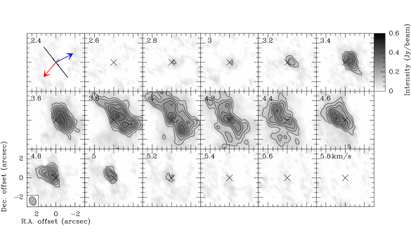
Figure 22: Channel maps of the C¹⁸O (2$-$1) emission from PdBI in L1448-2A. In the first panel, the outflow directions are shown by blue and red solid arrows and the equatorial axis is represented by a solid black line. The clean beam is shown by an ellipse on the bottom left. Contours are drawn in black solid lines at 5$\sigma$, 7$\sigma$ and so on. The systemic velocity is estimated to be $\mathrm{v}_{\mathrm{sys}}=$4.0 km s^-1 (see Table 15).

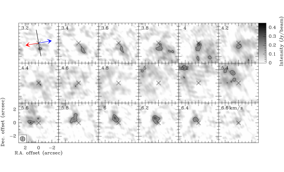
Figure 25: Same as Figure 22, but for L1448-NB. The systemic velocity is estimated to be $\mathrm{v}_{\mathrm{sys}}=$4.6 km s^-1 (see Table 15).

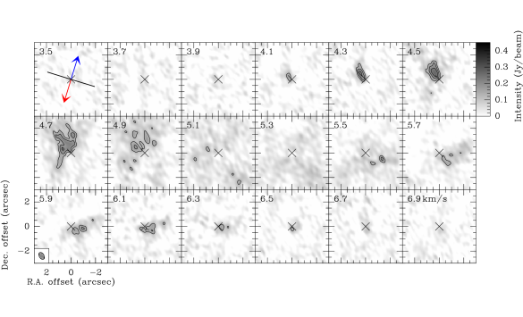
Figure 29: Same as Figure 22, but for L1448-C. The systemic velocity is estimated to be $\mathrm{v}_{\mathrm{sys}}=$5.1 km s^-1 (see Table 15).

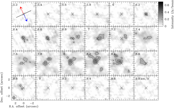
Figure 33: Same as Figure 22, but for IRAS2A. The systemic velocity is estimated to be $\mathrm{v}_{\mathrm{sys}}=$7.6 km s^-1 (see Table 15).

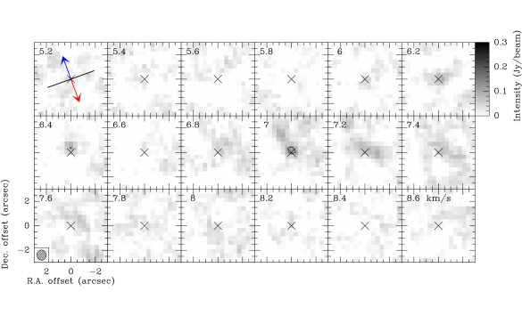
Figure 48: Same as Figure 22, but for IRAM04191. The systemic velocity is estimated to be $\mathrm{v}_{\mathrm{sys}}=$6.6 km s^-1 (see Table 15).

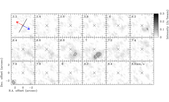
Figure 52: Same as Figure 22, but for L1521F. The systemic velocity is estimated to be $\mathrm{v}_{\mathrm{sys}}=$6.55 km s^-1 (see Table 15).

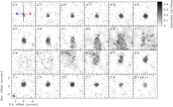
Figure 56: Same as Figure 22, but for L1527. The systemic velocity is estimated to be $\mathrm{v}_{\mathrm{sys}}=$5.8 km s^-1 (see Table 15).

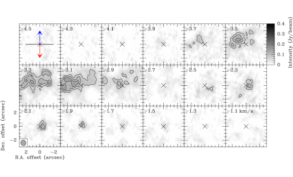
Figure 64: Same as Figure 22, but for GF9-2. The systemic velocity is estimated to be $\mathrm{v}_{\mathrm{sys}}=$-2.8 km s^-1 (see Table 15).

Seven sources in our sample show a small-scale velocity gradient aligned along the equatorial axis in C¹⁸O emission: L1448-2A, L1448-NB, L1448-C, IRAS2A, SVS13-B, L1527, and GF9-2 (see Figs. 22, 25, 29, 33, 37, 56, and 64, respectively). For IRAM04191 and L1521F (see Figures 48 and 52, respectively), the weak detection in C¹⁸O emission from the PdBI datasets does not allow the diagram to be constrained to the smallest scales of the envelope ($r<$60 au). For IRAS4A, IRAS4B, and L1157 (see Figures 42, 44, and 60, respectively), the channel maps do not exhibit an organized spatial distribution of velocities along the equatorial axis at $r\lesssim$350 au: the central emission fit show a position angle $>$—45${}^{\circ}|$ with respect to the equatorial axis, suggesting a contamination by the outflow kinematics. However, PdBI velocity maps exhibit weak gradients along the equatorial axis but working with the visibilities does not allow us to disentangle it from the emission from the outflows. Thus, for these three sources, we analyzed the PdBI observations in the image plane as described in the next section to constrain the PV_rot diagrams at scales of $r<$600 au.

C.2 Analysis of combined and 30m datasets in the image plane

We analyze the combined and 30m datasets in the image plane to probe the intermediate and outer scales of the envelope. For the pixel (i.e., a position) along the equatorial axis, we report the centroid velocity determined in the velocity maps in Sect. 4.2. The errors on the velocity given by the Gaussian or HFS functions are reported on the PV_rot diagrams (see Fig. 16 and Appendix H). The position errors are related to the pixel size, which is itself related to the spatial resolution of the datasets.

To build PV_rot diagrams we only consider the velocity gradients with blue and red-shifted components with respect to the systemic velocity, centered on the central protostar and along the equatorial axis axis as expected from rotational motions. The values from velocity maps that do not exhibit such an organized spatial distribution of velocities are considered as upper limits on the rotational velocity. Another requirement is the robustness of the centroid velocity offset with respect to the systemic velocity. We only considered spectra with a signal-to-noise ratio higher than 5. From a Gaussian measurement, we assume the centroid velocity cannot be robustly determined with an accuracy better than one third of the spectral resolution: we only consider the C¹⁸O points where the relative centroid velocity, $\mathrm{v}-\mathrm{v}_{\mathrm{lsr}}$, is $\geq\frac{\Delta\mathrm{v}}{3}$, with $\Delta\mathrm{v}$ the spectral resolution. From a HFS measurement, the centroid velocity is determined much more precisely thanks to the larger number of components: we only consider the N₂H⁺ points where $\mathrm{v}-\mathrm{v}_{\mathrm{lsr}}\geq\frac{\Delta\mathrm{v}}{3\times\sqrt{6}}$. We note that the weakest component which is 7 times weaker than the strongest one is never detected with a signal-to-noise ratio higher than 2 in the spectra.

C.3 Construction method of PV_rot diagrams

The analysis described above allows us to determine the centroid position of the emission at a given velocity and the centroid velocity at a given position, respectively. By putting the results end-to-end, we build a PV_rot diagram with a high dynamic range from 50 au up to 5000 au for each source as follows (see the example of L1448-C in Fig. 15):
$\bullet$ At the smallest scales resolved by our dataset ($\sim$0.5^′′) and up to the PdBI C¹⁸O emission size radius of the sources $R_{i}$ (see Tables 9 and 11, and Fig. 15), we use the PdBI C¹⁸O datasets to constrain the PV_rot diagram (see label ”C¹⁸O PdBI” in Fig. 15).
$\bullet$ Since the C¹⁸O extended emission is filtered out by the interferometer, we used the combined C¹⁸O emission to populate the PV_rot diagram at angular radii between $R_{i}$ and the 30m half-power beam width (HPBW $\sim$6^′′ at the C¹⁸O frequency, see Table 7). However, because the C¹⁸O molecule freezes onto dust ice mantles at temperatures below $\sim$20K, the maximum radius up to which it remains the best tracer of the inner envelope can be smaller than the 30m HPBW. To determine the maximal radius $R_{\mathrm{trans}}$ where the C¹⁸O molecule remains the best tracer, we calculate the C¹⁸O and N₂H⁺ column densities along the equatorial axis from the combined integrated intensity maps (see Appendix D and green points in Fig. 15). $R_{\mathrm{trans}}$ is defined one of the following criteria, depending on the source (see Table 11):
(i) the radius from which the C¹⁸O column density changes from a smooth decreasing profile to a noisy dispersion,
(ii) the maximum radius where the C¹⁸O emission is detected with a signal-to-noise ratio higher than 5 along the equatorial axis,
(iii) the radius below which the N₂H⁺ column density no longer traces the inner region and the profile flattens,
(iv) the radius where the N₂H⁺ profile reaches its maximum in column density.
For most sources, $R_{\mathrm{trans}}$ is smaller than the 30m HPBW. We used the combined C¹⁸O emission map to constrain the gas kinematics in the PV_rot diagram up to R_trans (see label ”C¹⁸O combined” in Fig. 15).
$\bullet$ At radii $r>R_{\mathrm{trans}}$, the N₂H⁺ emission traces better the envelope dense gas. We use the combined N₂H⁺ emission maps to analyze the envelope kinematics at intermediate scales, from $R_{\mathrm{trans}}$ to the 30m HPBW ($\sim$14^′′ at the N₂H⁺ frequency, see Table 8). However, the N₂H⁺ column density profile can reach a minimum value at radii $R_{\mathrm{trans}}<r<$ 30m HPBW due to the sensitivity of the combined datasets. In this case, the combined dataset is no longer the better dataset to provide a robust information on the velocity. We defined $R_{\mathrm{int}}$ the maximum radius up to which we use N₂H⁺ emission from the combined dataset (see Table 11 and see label ”N₂H⁺ combined” in Fig. 15).
$\bullet$ Beyond $R_{\mathrm{int}}$, we use the 30m N₂H⁺ emission map to populate the PV_rot diagram up to the largest scales of the envelope (see label ”N₂H⁺ 30m” in Fig. 15). We note $R_{\mathrm{out}}$ the maximum radius of the protostellar envelopes (see Table 11).

The sources in our sample show specific individual behaviors, therefore we adapted the method of building the PV_rot diagram described above on a case-by-case basis. Nevertheless we respected the transition radii as closely as possible (see Table 11).

Table 11: Transition radii between the different datasets (PdBI, combined, and 30m) and the two C¹⁸O and N₂H⁺ tracers used to build a high dynamic range position-velocity diagram for sources from the CALYPSO survey.

Source	C18O (2$-$1)					N2H+ (1$-$0)
	$R_{\mathrm{i}}$		$R_{\mathrm{trans}}$			$R_{\mathrm{int}}$		$R_{\mathrm{out}}$
	(′′)	(au)	(′′)	(au)		(′′)	(au)	(′′)	(au)
L1448-2A	1.4	410	4.2	1230	(iii)	13.9	4070	18$\pm$5	5270$\pm$1470
L1448-NB	1.6	470	5.9	1730	(iii)	13.9	4070	33$\pm$5	9670$\pm$1470
L1448-C	1.0	290	3.5	1230	(iii)	13.9	4070	25$\pm$2	7320$\pm$590
IRAS2A	1.6	470	5.1	1490	(i)	9	2640	34$\pm$6	9960$\pm$1760
SVS13-B	0.5	145	2.0	590	(i)	7	2050	7$\pm$3	2050$\pm$880
IRAS4A ⋆	2.6	760	3.1	910	(i)	5.5	1610	5.9$\pm$1.0	1730$\pm$ 290
IRAS4B ⋆	1.5	440	2.1	615	(ii)	3.5	1030	11$\pm$2	3220$\pm$590
IRAM04191	…	…	5.6	780	(iv)	13.9	1950	100$\pm$11	14000$\pm$1540
L1521F ⋆⋆	0.5	70	5.9	820	…	…	…	32$\pm$3	4480$\pm$420
L1527	1.1	150	3.3	460	(ii)	13.9	1950	$>$121	$>$16940
L1157	0.8	280	1.8	630	(ii)	13.9	4890	45$\pm$5	15840$\pm$1760
GF9-2	1.9	380	5.1	1020	(i)	…	…	35$\pm$5	7000$\pm$1000

Appendix D Details of column density estimate

To interpret the gas kinematics using both C¹⁸O and N₂H⁺ emission in a robust way, it is important to constrain from which scales in the envelope their emission comes from. This is especially important because we merged single-dish and interferometric datasets which are sensitive to different scales of the envelope (see Tables 9 and 10). Therefore, we built column density maps to quantify the scales probed by C¹⁸O and N₂H⁺ molecular lines. We assumed that the observed molecular transitions are optically thin ($\tau_{\nu}<<$1) and we used Eq. (3) defined in Mangum & Shirley (2015):

$$N_{thin}\leavevmode\nobreak\ =\leavevmode\nobreak\ \frac{3\leavevmode\nobreak\ k}{8\leavevmode\nobreak\ \pi^{3}\leavevmode\nobreak\ \mu^{2}\leavevmode\nobreak\ B_{\mathrm{0}}\leavevmode\nobreak\ R_{\mathrm{i}}}\leavevmode\nobreak\ (T_{\mathrm{ex}}+\frac{hB}{3k})\leavevmode\nobreak\ \frac{\exp(\frac{E_{\mathrm{u}}}{T_{\mathrm{ex}}})}{\exp(\frac{h\nu}{kT_{\mathrm{ex}}})-1}\leavevmode\nobreak\ \leavevmode\nobreak\ \frac{\int T_{\mathrm{R}}\,\mathrm{d}v}{\mathrm{J}_{\nu}(T_{\mathrm{ex}})-\mathrm{J}_{\nu}(T_{\mathrm{bg}})},$$ (3)

where $E_{\mathrm{u}}$ is the energy of the upper level, $\mu$ is the dipole moment of the molecule, $B_{\mathrm{0}}$ the rotational constant, $h$ Planck’s constant, $k$ Boltzmann’s constant, $R_{\mathrm{i}}$ the relative intensity of the component if the transition has a hyperfine structure, $T_{\mathrm{ex}}$ the excitation temperature, and $T_{\mathrm{bg}}$ the cosmic background temperature (Mather et al. 1994). $\mathrm{J}_{\nu}$ is the effective radiation temperature defined by $\mathrm{J}_{\nu}(T)=\frac{h\nu}{k}\leavevmode\nobreak\ \frac{1}{\exp(\frac{h\nu}{kT})-1}$. We report the values of each parameter for the two emission lines in Table 12.

Table 12: Parameters used to determine the column density of the C¹⁸O and N₂H⁺ molecules from Eq. (3).

Parameter	N2H+	C18O
$\nu$ (MHz)	93176.2595	219560.3541
$E_{u}$ (K)	4.47172	15.8058
$\mu$ (Debye)	3.40	0.11049
$B_{\mathrm{0}}$ (MHz)	46586.87	54891.42
$R_{\mathrm{i}}$	$\frac{3}{27}$	1

Assuming local thermodynamical equilibrium (LTE), we can determine the excitation temperature from the gas temperature within the emission size of each tracer observed in the combined dataset (see Table 11). This hypothesis is valid when the density is higher than the critical density of the transition of C¹⁸O (2$-$1) and N₂H⁺ ($1_{01}-0_{12}$), estimated at $\sim$ 8.4 $\times$ 10³ cm^-3 (Flower 2001) and $\sim$2.6 $\times$ 10⁵ cm^-3 (Daniel et al. 2005), respectively at $T\sim$10 K. Belloche et al. (2002) estimate for IRAM04191, one of the lowest envelope masses of our sample (see Table 2), a density higher than 10⁵ cm^-3 up to $r\sim$4000 au. Thus, LTE is a good assumption for both transitions in our sample. As the dust temperature in the envelope is a good approximation for the gas kinetic temperature (Ceccarelli et al. 1996), we used dust temperature profiles from CALYPSO PdBI observations assuming that the temperature distribution depends on the radius $r$ from the central stellar object and the internal luminosity of the source $L_{\mathrm{int}}$ (see Table 2) as follows (Terebey et al. 1993):

$$T_{\mathrm{dust}}(r)=60\leavevmode\nobreak\ \times\leavevmode\nobreak\ \left(\frac{r}{13400\leavevmode\nobreak\ au}\right)^{-q}\leavevmode\nobreak\ \left(\frac{L_{\mathrm{int}}}{10^{5}L_{\odot}}\right)^{q/2},$$ (4)

with $q=0.4$ for the CALYPSO sample (Terebey et al. 1993; Maury et al. 2019). We weighted the radial temperature distribution with the dust column density as a function of $r$, that is the amount of material at each radius, to estimate a single robust mean value of gas temperature (see Table 13). For C¹⁸O, we used the PdBI flux at 1.3 mm calculated at different radii by Maury et al. (2019). For N₂H⁺, we assumed a density profile of $\rho\propto r^{-p}$, with the index $p$ equal to the values determined at 3 mm by Maury et al. (2019). The excitation temperature values adopted for each source to derive the column density are given in Table 13. There are two exceptions in the CALYPSO sample: IRAM04191 and L1521F, which have the lowest luminosities of the CALYPSO sample (see Table 2). The dust temperature profile of these sources from the PdBI dataset cannot be determined because the temperature profile is dominated by external heating. Belloche et al. (2002) and Tokuda et al. (2014, 2016) estimate the dust temperature at $\sim$10 K at scales $\sim$2000 au. From Eq. (4) and from values of $L_{\mathrm{int}}$ estimated for these two sources (0.05 L_⊙ for IRAM04191, André et al. 2000, and 0.035 L_⊙ for L1521F, Tokuda et al. 2016) we determined mean excitation temperatures of 20 K for the C¹⁸O molecule and 10 K for the N₂H⁺ molecule (see Table 13).

We note that we did not use the excitation temperature determined by fitting the HFS line profile for the N₂H⁺ molecule. For most sources in the CALYPSO sample, the average spectrum from the combined dataset within the central 14$\hbox{${}^{\prime\prime}$}\times$14^′′ does not follow the relative intensities of the hyperfine components expected under LTE conditions (3,3,7,5,3,5,1 from the isolated hyperfine component $1_{01}-0_{12}$; Endres et al. 2016). Thus, either the emission does not satisfy the LTE conditions or this is an effect of the partial opacity of emission. Moreover, some adjacent hyperfine components are too close to be spectroscopically separated despite the good spectral resolution of the combined dataset (0.13 km s^-1 at 3 mm). To minimize the error propagation, we only considered the isolated hyperfine component ($1_{01}-0_{12}$) to determine the N₂H⁺ column density (Caselli et al. 1995, 2002).

We determined the C¹⁸O (2$-$1) and N₂H⁺ ($1_{01}-0_{12}$) opacities for our source sample assuming optically thin emission and using the maximum temperature of the emission spectrum $T_{\mathrm{peak}}$:

$$\tau_{\nu}=\frac{T_{\mathrm{peak}}}{\mathrm{J}_{\nu}(T_{\mathrm{ex}})-\mathrm{J}_{\nu}(T_{\mathrm{bg}})}.$$ (5)

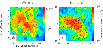
Figure 26: Same Figure as 21 for L1448-NB.

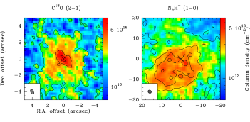
Figure 30: Same Figure as 21 for L1448-C.

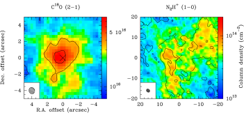
Figure 34: Same Figure as 21 for IRAS2A.

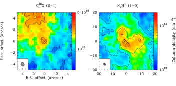
Figure 38: Same Figure as 21 for SVS13-B

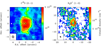
Figure 45: Same Figure as 40 for IRAS4B. The N₂H⁺ (1$-$0) column density maps is determined from the PdBI datasets. The integrated intensity overlaid in black solid line is the integrated intensity from the 7 hyperfine components of the transition (see top left panel on Figure 43)

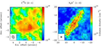
Figure 53: Same Figure as 21 for L1521F.

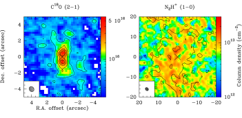
Figure 57: Same Figure as 21 for L1527.

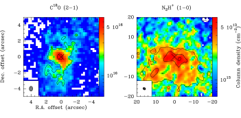
Figure 61: Same Figure as 21, but for L1157.

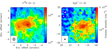
Figure 65: Same Figure as 21 for GF9-2.

We calculated the opacity on the spectra of each pixel from the combined dataset for both molecular transition. We used the excitation temperature values mentioned above and a standard value of the cosmic background temperature $T_{\mathrm{bg}}$=2.7 K (Mather et al. 1994). We report the average $\tau_{\nu}$ on the size of the combined maps of C¹⁸O and N₂H⁺ emissions (5^′′ $\times$ 5^′′ and 20^′′ $\times$ 20^′′, respectively) in Table 13. We noticed that the sources have average $\tau_{\nu}<$0.4 but some pixels have opacity values $>$0.5. We determined the column density from each pixel using Eq. (3) and the parameter values listed in Table 12 for the C¹⁸O and N₂H⁺ molecules. For the calculation of column density, we distinguished two opacity regimes according to the value of $\tau_{\nu}$ of each spectrum:
$\indent\bullet$ an optically thin regime where $\tau_{\nu}<$0.4 : in this case, the density column is determined by Eq. (3),
$\indent\bullet$ an intermediate regime where $\tau_{\nu}\geq$0.4 : in this case, the optically thin hypothesis is no longer a reasonable hypothesis and a correction factor $\frac{\tau_{\nu}}{1-e^{-\tau_{\nu}}}$ (Goldsmith & Langer 1999) must be applied to the Eq. (3) to calculate the column density. Indeed, the column density determined in the optically thin hypothesis by Eq. (3) is underestimated by more than 20% for a value of $\tau_{\nu}=$0.4.
Figure 21 shows as an example the column density maps from the combined dataset obtained for L1448-2A. The column density maps of the other sources from our sample are provided in Appendix H (see Figs. 26, 30, 34, 38, 40, 45, 49, 53, 57, 61, and 65).

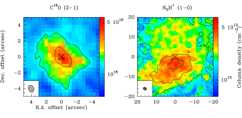
Figure 21: Column density maps of C¹⁸O (2$-$1) (left) and N₂H⁺ (1$-$0) (right) emission from the combined dataset for L1448-2A. The black cross represents the middle position between the binary protostars determined with the 1.3 mm dust continuum emission. The N₂H⁺ column density map was determined from the isolated hyperfine component ($1_{01}-0_{12}$) but the contours represent the integrated intensity of the 7 hyperfine components. The integrated intensity contours in black are the same as in Fig. 1.

Table 13: Mean column density of C¹⁸O and N₂H⁺ and opacity of the transitions (2$-$1) and (1$-$0), respectively determined from the combined dataset for the CALYPSO sample sources.

Source	C18O (2$-$1)			N2H+ (1$-$0)
	$T_{\mathrm{ex}}$	$N_{\mathrm{mean}}$	$\tau_{\mathrm{mean}}$	$T_{\mathrm{ex}}$	$N_{\mathrm{mean}}$	$\tau_{\mathrm{mean}}$
	(K)	(1015 cm-2)		(K)	(1013 cm-2)
L1448-2A	39	13.4	0.22	20	2.2	0.09
L1448-NB	33	17.2	0.37	19	3.3	0.16
L1448-C	61	20.3	0.18	26	2.1	0.06
IRAS2A	58	23.5	0.17	33	4.3	0.06
SVS13-B	40	13.4	0.17	24	3.9	0.10
IRAS4A	33	16.5	0.30	24	0.6	0.03
IRAS4B	39	9.5	0.14	25	0.4	0.03
IRAM04191	20	3.5	0.17	10	0.6	0.10
L1521F	20	3.6	0.22	10	1.5	0.33
L1527	37	5.4	0.13	19	0.7	0.05
L1157	38	8.1	0.19	25	2.2	0.05
GF9-2	43	4.2	0.09	21	1.2	0.05

Appendix E Systemic velocity estimate

The systemic velocities of the sources are the reference velocities to quantify centroid velocity variations in the PV_rot diagrams. The systemic velocity is defined as the average velocity of an object. The linear velocity gradient modeling allows us to determine a systemic velocity, $\mathrm{v}_{0}$, in the different datasets and tracers. For a given source, we noticed that $\mathrm{v}_{0}$ is different depending on the region of the envelope considered (see Table 2).

In the first place, we determine these values by fitting the HFS line profile of the optically thin transition N₂H⁺ (1$-$0) from the 30m datasets. Table 14 reports these first estimates and compares them to the values found in the literature. The differences of a few tenths of a km s^-1 between our values and the literature can be explained by the different tracers used in our study compared to the literature. Indeed, different tracers do not trace exactly the same material in the protostellar envelopes, as we observed with the C¹⁸O and N₂H⁺ in our study (see Sect. 4.2 and Table 2). There could also be systematic uncertainty on the rest frequencies or on the calibration of the spectral axis for instance. This first estimate in the quieter parts of the envelopes, could be more robust than a value determined in the inner parts which can be dominated by rotation, collapse, or ejection. On the other hand, the turbulence at large scales could affect the systemic velocity if the outer envelope is turbulent or if there is a contamination of the turbulence on the line of sight from cloud scales. In the case of an axisymmetric envelope with a symmetric kinematics (infall and rotation), the systemic velocity could be more accurate at small scales.

Table 14: Systemic velocity values determined from HFS fit on the average spectrum N₂H⁺ from CALYPSO 30m dataset compared to the literature.

Source	$\mathrm{v}_{\mathrm{sys}}^{\mathrm{30m}}$	$\mathrm{v}_{\mathrm{sys}}^{\mathrm{literature}}$
	(km s-1)	(km s-1)
L1448-2A	4.10 $\pm$ 0.04	4.20
L1448-NB	4.47 $\pm$ 0.02	4.70
L1448-C	4.73 $\pm$ 0.03	5.00
IRAS2A	7.60 $\pm$ 0.04	7.30
SVS13-B	8.02 $\pm$ 0.02	8.40
IRAS4A	7.34 $\pm$ 0.03	7.24
IRAS4B	7.20 $\pm$ 0.06	7.00
IRAM04191	6.63 $\pm$ 0.06	6.66
L1521F	6.47 $\pm$ 0.01	6.45
L1527	5.89 $\pm$ 0.01	5.90
L1157	2.65 $\pm$ 0.03	2.65
GF9-2	-2.56 $\pm$ 0.02	-2.60

(1) Tobin et al. (2007); (2) Kwon et al. (2006); (3) Jørgensen et al. (2007); (4) Codella et al. (2014b); (5) Chen et al. (2009); (6) Belloche et al. (2006); (7) Anderl et al. (2016); (8) Jørgensen & van Dishoeck (2010); (9) Belloche et al. (2002); (10) Tobin et al. (2011); (11) Bachiller & Pérez Gutiérrez (1997); (12) Goodman et al. (1993).

If the reference velocity value is well chosen, blue- and red-shifted velocity points should overlap if the envelope is axisymmetric. In practice, the gradients may not be symmetric with respect to the central position of the source. This asymmetry can cause shifts in position between the blue-shifted and the red-shifted emission. We built the PV_rot diagrams by maximizing the overlap between blue- and red-shifted velocity points to produce the best symmetric pattern. We applied this method independently for the PV_rot diagram points from the C¹⁸O and N₂H⁺ emission to determine the best couple ($\mathrm{v}_{\mathrm{sys}}$, $r_{\mathrm{orig}}$) adapted to each tracer, with $\mathrm{v}_{\mathrm{sys}}$ the systemic velocity and $r_{\mathrm{orig}}$ the central position of the gradient along the equatorial axis. We fit a power-law function (see Sect. 5.1) exploring a range of $\pm$0.7 km s^-1 around the first estimate of the systemic velocity determined at outer envelope scales and a range of $\pm$0.2^′′ along the equatorial axis around the dust continuum peak (see Table 2). Table 15 gives the reduced $\chi^{2}$ associated with the best couple of parameters corresponding to the best overlap of the blue- and red-shifted points. This method does not allow for a more accurate determination of the systemic velocity value than 0.05 km s^-1 given the errors on the velocity of the points populating the PV_rot diagrams. We therefore added a systematic error of 0.05 km s^-1 to previous velocity errors determined above for both tracers. The central positions and systemic velocities obtained with this method are on average within $<$0.2 km s^-1 and $<$0.1^′′of the first estimates of these values using the average N₂H⁺ spectrum (see Sect. E and Table 14) and the dust continuum peak (see Table 2).

Table 15: Values of systemic velocity and central position giving the best overlap and $\chi^{2}$ by independent fits of C¹⁸O and N₂H⁺ points.

Source	Line	$v_{\mathrm{sys}}$	$r_{\mathrm{orig}}$ coordinates		Power law fit
			R.A.	DEC	$\eta$	$\chi^{2}$
		(km s-1)	(h:m:s) (J2000)	(∘:$\arcmin$:′′) (J2000)
L1448-2A	C18O	4.0 (-0.1)	03:25:22.380 (+0.06′′)	30:45:13.28 (+0.08′′)	-0.9 $\pm$0.1	1.4
	N2H+	$u$	$u$	$u$	…	…
L1448-NB	C18O	4.6 (+0.1)	03:25:36.316 (+0.01′′)	30:45:15.10 (-0.05′′)	-0.94 $\pm$0.04	2.3
	N2H+	…	…	…	…	…
L1448-C	C18O	5.1 (+0.4)	$u$	$u$	-1.0 $\pm$0.1	1.4
	N2H+	4.9 (+0.2)	$u$	$u$	0.8 $\pm$0.1	3.0
IRAS2A	C18O	$u$	$u$	$u$	-0.7 $\pm$ 0.1	0.2
	N2H+	…	…	…	…	…
SVS13-B	C18O	8.3 (+0.3)	$u$	$u$	-0.9$\pm$ 0.3	0.2
	N2H+	…	…	…	…	…
IRAS4A	C18O	6.6 (-0.7)	$u$	$u$	0.2$\pm$0.2	1.8
	N2H+	6.8 (-0.5)	$u$	$u$	0.6$\pm$0.3	0.7
IRAS4B	C18O	6.9 (-0.3)	$u$	$u$	-0.3 $\pm$0.4	0.5
	N2H+	7.0 (-0.2)	$u$	$u$	-2.0 $\pm$2.2	0.1
IRAM04191	C18O	$u$	$u$	$u$	-0.2 $\pm$ 0.2	0.3
	N2H+	…	…	…	…	…
L1521F	C18O	6.55 (+0.1)	$u$	$u$	0.2 $\pm$ 0.5	0.1
	N2H+	…	…	…	…	…
L1527	C18O	5.8 (-0.1)	$u$	$u$	-1.07 $\pm$ 0.04	1.5
	N2H+	$u$	$u$	$u$	0.4 $\pm$0.4	0.7
L1157	C18O	$u$	$u$	$u$	0.1 $\pm$0.3	0.3
	N2H+	…	…	…	…	…
GF9-2	C18O	-2.8 (-0.2)	20:51:29.836 (+0.2 ′′)	60:18:38.44 (+0′′)	-0.8 $\pm$0.1	1.8
	N2H+	…	…	…	…	…

Appendix F Details on $j$ distributions

Table 16: Parameters from best fits by power-law or broken power-law functions of specific angular momentum distribution $j$.

Source	Radial range	Power law fit		Broken power law fit
		$\beta$	$\chi^{2}$	$\beta_{r<r_{\mathrm{break}}}$	$r_{\mathrm{break}}$	$\beta_{r>r_{\mathrm{break}}}$	$\chi^{2}$
	(au) $-$ (au)				(au)
L1448-2A	60$-$1250	0.1 $\pm$ 0.1	1.4	…	…	…	…
L1448-NB	150$-$1700	0.07 $\pm$ 0.04	2.4	-0.3 $\pm$ 0.1	630 $\pm$ 80	0.9 $\pm$ 0.2	0.8
L1448-C	100$-$4000	-0.01 $\pm$ 0.08	1.6	-0.1 $\pm$ 0.1	509 $\pm$ 105	1.0 $\pm$ 0.3	1.0
IRAS2A	85$-$1500	0.3 $\pm$ 0.1	0.2	…	…	…	…
SVS13-B	110$-$450	0.1 $\pm$ 0.3	0.2	…	…	…	…
IRAS4B	175$-$1050	0.4 $\pm$ 0.3	0.5	…	…	…	…
IRAM04191	55$-$800	0.7 $\pm$ 0.2	0.2	…	…	…	…
L1521F	1500$-$4200	1.2 $\pm$ 0.6	0.1	…	…	…	…
L1527	45$-$2000	-0.13 $\pm$ 0.03	1.6	…	…	…	…
L1157	85$-$650	1.1 $\pm$ 0.4	0.2	…	…	…	…
GF9-2	75$-$850	0.3 $\pm$ 0.1	1.6	…	…	…	…
Median profile	45$-$4200	1.0 $\pm$ 0.2		0.4$\pm$0.6	1030$\pm$500	1.4$\pm$0.3

Table 17: Same as Table 16 for the distribution of apparent specific angular momentum —$j_{\mathrm{app}}$— along the equatorial axis.

Source	Radial range	Power law fit		Broken power law fit
		$\beta_{\mathrm{app}}$	$\chi^{2}$	$\beta_{\mathrm{app},r<r_{\mathrm{break}}}$	$r_{\mathrm{\mathrm{app},break}}$	$\beta_{\mathrm{app},r>r_{\mathrm{break}}}$	$\chi^{2}$
	(au) $-$ (au)				(au)
L1448-2A	60$-$4000	0.3 $\pm$ 0.1	1.3	0.1 $\pm$ 0.1	1380 $\pm$ 400	1.6 $\pm$ 0.5	0.6
L1448-NB	150$-$8200	0.02 $\pm$ 0.04	2.3	…	…	…	…
L1448-C	100$-$4000	0.69 $\pm$ 0.03	5.5	-0.1 $\pm$ 0.1	790 $\pm$ 100	1.6 $\pm$ 0.1	2.0
IRAS2A	85$-$8200	1.4 $\pm$ 0.1	6.2	0.3 $\pm$ 0.1	2180$\pm$110	28.4 $\pm$ 22.2	2.5
SVS13-B	110$-$1900	1.0 $\pm$ 0.1	1.5	0.1 $\pm$ 0.3	640$\pm$190	2.2 $\pm$ 0.5	0.2
IRAS4A	250$-$1600	1.9 $\pm$ 0.1	0.9	-0.3 $\pm$ 0.7	470$\pm$60	2.1$\pm$0.2	0.4
IRAS4B	175$-$3100	1.5 $\pm$ 0.1	4.0	…	…	…	…
IRAM04191	55$-$9700	0.8 $\pm$ 0.1	0.5	…	…	…	…
L1521F	1500$-$4200	1.2 $\pm$ 0.6	0.1	…	…	…	…
L1527	45$-$7800	-0.12 $\pm$ 0.03	1.8	-0.14 $\pm$ 0.03	1320 $\pm$ 260	1.3 $\pm$ 0.2	1.6
L1157	85$-$9800	0.8 $\pm$ 0.1	0.4	…	…	…	…
GF9-2	75$-$5600	0.5 $\pm$ 0.1	2.3	0.3 $\pm$ 0.1	980 $\pm$ 370	1.2 $\pm$ 0.3	1.0
Median profile	45$-$9800	0.9 $\pm$ 0.1		0.3$\pm$0.3	1570$\pm$300	1.6$\pm$0.2

Appendix G Details on linewidth distributions

Table 18: Parameters from best fits by power-law functions of linewidth distribution $D\mathrm{v}$ in the outer envelope.

Source	Outer envelope	Power law fit
	(au)	$\gamma$	$\chi^{2}$
L1448-2A	$r>$1380	-0.9 $\pm$ 0.2	8.0
L1448-NB	$r>$630	0.3 $\pm$ 0.1	30.2
L1448-C	$r>$790	0.2 $\pm$ 0.1	16.7
IRAS2A	$r>$2180	0.1 $\pm$ 0.2	65.3
SVS13-B	$r>$640	0.17 $\pm$ 0.04	2.5
IRAS4A	$r>$470	0.7 $\pm$ 0.4	34.1
IRAS4B	$r>$0	-0.3 $\pm$ 0.1	33.1
IRAM04191	$r>$850	-0.2 $\pm$ 0.1	16.3
L1521F	$r>$1000	1.1 $\pm$ 0.6	7.3
L1527	$r>$1320	-0.2 $\pm$ 0.1	14.1
L1157	$r>$1420	0.6 $\pm$ 0.1	13.0
GF9-2	$r>980$	0.16 $\pm$ 0.04	0.3

Appendix H Comments on individual sources

H.1 L1448-2A

L1448-2A (also known as L1448-IRS2 or Per-emb-22) is a Class 0 protostar in the L1448N complex in the Perseus cloud at a distance previously estimated to be 235 pc (Hirota et al. 2011) but determined at (293 $\pm$ 20) pc by recent Gaia parallax measurements (Ortiz-León et al. 2018). CO emission maps showed the presence of a bipolar flow in the northwest-southeast direction (O’Linger et al. 1999). Another study by Wolf-Chase et al. (2000) suggests that the source shows distinct bipolar outflows, namely a signature of the presence of a binary system. Observations with VLA confirmed that L1448-2A is a binary system separated by $\sim$170 au (Tobin et al. 2016b). 1.3 mm dust continuum emission also resolves the binary system with a separation of $\sim$180 au (Maury et al. 2019, see Table 2). Podio & CALYPSO (in prep.) report two angle values (+63^∘ (blue), +140^∘ (red), see Table 2) because the observed red and blue flow cavities are not aligned.

Figures 1 and 3 show the integrated intensity and centroid velocity maps obtained for this source from the PdBI, combined, and 30m CALYPSO datasets for the C¹⁸O and N₂H⁺ emission respectively. The C¹⁸O emission from the PdBI datasets does not peak on the main protostar L1448-2A1 but in the middle of the binary system (see Table 2 and Figure 1). Thus, the origin of the coordinate offsets is chosen to be the middle of the binary system (RA: 03^h25^m22^s.380, Dec.: 30^∘45$\arcmin$13^′′.21; see Table 2) to study the kinematics in the protostellar envelope of L1448-2A.

The gradients observed in the PdBI and combined velocity maps of the C¹⁸O emission (see bottom left and middle panels on Figure 3) have an orientation of 99${}^{\circ}\leq\Theta\leq$107^∘, they show a difference $>$60^∘ with respect to the equatorial axis (see Table 2). Therefore, these gradients at $r<$700 au are a merging of the kinematics between several mechanisms: ejection by outflows, orbital motions of the binary system, and rotational motions of the envelope along the equatorial axis. The N₂H⁺ emission from the PdBI datasets (see top left panel on Figure 3) shows reversed gradients at scales of $r\sim$2000 au with respect to those observed at smaller scales ($\Theta\sim$-87^∘, see Table 2). In the outer envelope (see top middle and right panels on Figure 3), the velocity gradients are not continuous in the same direction and not source-centered. Therefore, these gradients seem to be due to an external contamination. We notice that the gradients from the 30m datasets at scales of $r>$4500 au (see right top and bottom panels on Figure 3) have a PA of -8$-$14^∘ and are in the opposite to the direction of the bipolar outflows (see Table 2). Moreover, the integrated intensity at these scales seems to trace an elongated structure from east to west that could be compatible with part of the filament.

The panel (a) of Fig. 16 shows the PV_rot diagram of L1448-2A built from the velocity gradients observed at scales of $r<$1300 au. The index of the fitting by a power-law ($\alpha\sim$-0.9, see Table 3) is consistent with an infalling and rotating protostellar envelope. Therefore, we constrain the radial distribution of the specific angular momentum of L1448-2A at radii of 60$-$1300 au (see Figure 23).

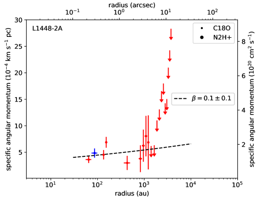
Figure 23: Radial distribution of specific angular momentum along the equatorial axis for L1448-2A. Blue and red dots show the blue- and red-shifted rotational velocities, respectively. Dots and large dots show points from C¹⁸O and N₂H⁺ emission, respectively. The arrows display upper limits of $j$ determined from velocity maps that do not exhibit a spatial distribution of velocities as organized as one would expect from rotation motions (see Sect. 4.3 and Appendix C). The dashed line shows the best least-square fitting with a power-law model leaving the index $\beta$ as a free parameter ($j\propto r^{\beta}$).

H.2 L1448-NB

L1448-NB (or L1448-IRS3) is a Class 0 protostar in the L1448N complex in the Perseus cloud at (293 $\pm$ 20) pc (Ortiz-León et al. 2018). This source is part of a multiple system: L1448-NA, L1448-NB, and L1448-NC. NA and NB are separated by 1700 au, and NB and NC are separated by 4900 au (Maury et al. 2019). L1448-NB is itself also a multiple system: Maury et al. (2019) find a binary system with a separation of $\sim$140 au. ALMA 1.3 mm observations with an angular resolution of $\sim$0.2^′′ showed L1448-NB as a triple protostar system with binaries separated by $\sim$60 au and a third core separated by $\sim$180 au from others (Tobin et al. 2016a).

Figures 24 and 4 show the integrated intensity and centroid velocity maps obtained for L1448-NB from the PdBI, combined, and 30m CALYPSO datasets for the C¹⁸O and N₂H⁺ emission respectively. The C¹⁸O emission from the PdBI dataset does not peak on the main protostar L1448-NB1 but on the secondary NB2 resolved by 1.3 mm continuum emission of the binary system (see Table 2 and Figure 24). Thus, the origin of the coordinate offsets is chosen to be the secondary protostar NB2 of the binary system (RA: 03^h25^m36^s.315, Dec.: 30^∘45$\arcmin$15^′′.15; see Table 2) to study the kinematics in the protostellar envelope of L1448-NB.

The gradients observed in the PdBI and combined velocity maps of the C¹⁸O emission (see bottom left and middle panels on Figure 4) are along a northeast-southwest axis and have a PA of $\Theta\sim$50^∘, namely a difference $>$50^∘ with respect to the equatorial axis (see Table 2). Therefore, these gradients at $r<$1000 au are a merging of the kinematics between several mechanisms: ejection by outflows, orbital motions of the binary system NB1 and NB2, and rotational motions of the envelope along the equatorial axis. They are consistent with those observed from SMA observations of C¹⁸O emission by Lee et al. (2015) and Yen et al. (2015a). In the outer envelope at $r>$1000 au, velocity gradients are in the direction of the bipolar outflows. They have an angle of 64${}^{\circ}\leq\Delta\Theta\leq$90^∘ with respect to the equatorial axis (see Table 2). Therefore, these gradients are not dominated by rotational motions along the equatorial axis but by ejection motions from bipolar outflows or due to an external contamination.

The panel (b) of Fig. 16 shows the PV_rot diagram of L1448-NB built from the velocity gradients observed at scales of $r<$1700 au. The index of the fitting by a power-law ($\alpha\sim$-0.9, see Table 3) is consistent with an infalling and rotating protostellar envelope. Therefore, we constrain the radial distribution of the specific angular momentum of L1448-NB at radii of 150$-$1700 au (see Figure 27).

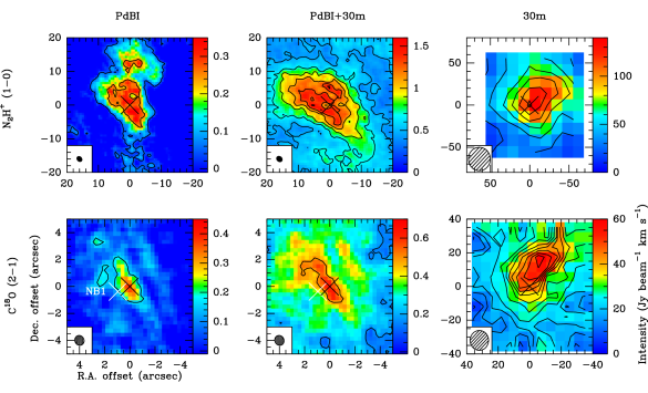
Figure 24: Same as Figure 1, but for L1448-NB. The white cross represents the position of main protostar L1448-NB1 determined from the 1.3 mm dust continuum emission (see Table 2). The black cross represents the position of the secondary protostar L1448-NB2 of the multiple system. The black lines represent the integrated intensity contours of each tracer starting at 5$\sigma$ and increasing in steps of 20$\sigma$ for N₂H⁺ and 10$\sigma$ for C¹⁸O (see Tables 9 and 10).

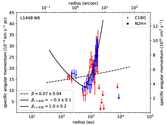
Figure 27: Same as Figure 23, but for L1448-NB. The dashed line shows the best least-square fitting with a power-law model ($j\propto r^{\beta}$) whereas the solid line shows the best least-square fitting with broken power-law.

H.3 L1448-C

L1448-C (or L1448-mm) is located in the Perseus molecular cloud at a distance of (293 $\pm$ 20) pc (Ortiz-León et al. 2018). This source was firstly detected as a radio source at 2 cm (Curiel et al. 1990) associated with a strong millimetric continuum emission (Bachiller et al. 1991). This Class 0 protostar (Barsony et al. 1998) has a powerful and very collimated outflow ($\sim$70 km s^-1; Bachiller et al. 1990; Guilloteau et al. 1992; Bachiller et al. 1995; Hirano et al. 2010). Podio & CALYPSO (in prep.) estimate the PA of this outflow at -17^∘ (see Table 2). Maret et al. (2020) detect for the first time hints of Keplerian rotation at scales of $r\sim$200 au.

Figures 28 and 5 show the integrated intensity and centroid velocity maps obtained for L1448-C from the PdBI, combined, and 30m CALYPSO datasets for the C¹⁸O and N₂H⁺ emission respectively. The gradients observed in the PdBI and combined velocity maps of the C¹⁸O emission (see bottom left and middle panels on Figure 5) have a PA of -140^∘ ¡ $\Theta$ ¡-121^∘, namely an angle difference $<$30^∘ with respect to the equatorial axis (see Table 2). This gradient is consistent with the one observed in C¹⁸O (2$-$1) emission with SMA (Yen et al. 2013, 2015b). The 30m datasets show no velocity gradient (see bottom right panel on Figure 5). From the N₂H⁺ emission (see top panels on Figure 5), we observed a clear velocity gradient with an orientation consistent with the outflow axis ($\Theta$ $\geq$152^∘, see Table 2). However, we detect a weak velocity gradient along the equatorial axis. The kinematics seems to be dominated by bipolar jets and outflows or by external contamination from scales $>$1500 au. Curiel et al. (1999) interpreted the gradient along the equatorial axis and the gradient along the outflows at larger scales as a suggestion that the envelope is rotating and contracting at similar velocities.

The panel (c) of Fig. 16 shows the PV_rot diagram of L1448-C built from the velocity gradients observed at scales of $r<$4000 au. The index of the fitting by a power-law ($\alpha\sim$-1, see Table 3) is consistent with an infalling and rotating protostellar envelope. From SMA observations, Yen et al. (2013) obtain an index $\alpha\sim$-1 on scales of 100$-$3000 au, consistent with our results. Figure 31 shows the radial distribution of the specific angular momentum of L1448-C at radii of 100$-$4000 au.

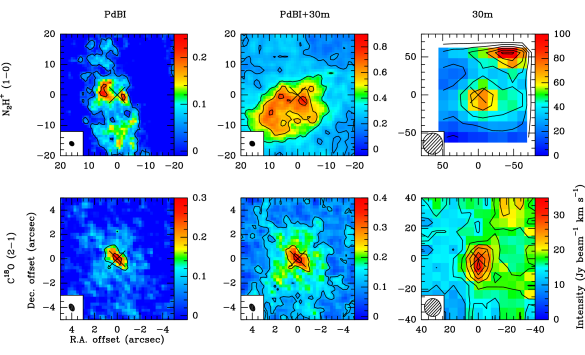
Figure 28: Same as Figure 1, but for L1448-C. The black lines represent the integrated intensity contours of each tracer starting at 5$\sigma$ and increasing in steps of 20$\sigma$ for N₂H⁺ and 5$\sigma$ for C¹⁸O (see Tables 9 and 10

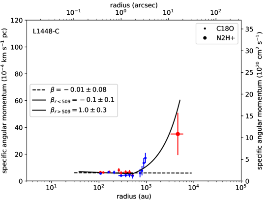
Figure 31: Same as Figure 23, but for L1448-C. The dashed line shows the best least-square fitting with a power-law model ($j\propto r^{\beta}$) whereas the solid line shows the best least-square fitting with broken power-law.

H.4 IRAS2A

IRAS2A (also known as NGC1333-IRAS2A) is located in the molecular cloud NGC1333 in the Perseus complex at (293 $\pm$ 20) pc (Ortiz-León et al. 2018). This Class 0 protostar was firstly detected via observations of dust continuum emission at 450 $\mu$m, 850 $\mu$m, and at 3 mm (Sandell et al. 1994; Sandell & Knee 2001; Jørgensen et al. 2004). The CO emission showed the presence of two bipolar outflows in the north-south east-west direction (Knee & Sandell 2000), suggesting the presence of a binary system. Dust continuum observations with VLA resolve IRAS2A into a protobinary system separated by $\sim$140 au (Tobin et al. 2015), which is not resolved by the CALYPSO observations (Maury et al. 2019). Codella et al. (2014a) and Podio & CALYPSO (in prep.) detect jet associated with the principal component with a PA of +205^∘ and a tentative SiO and SO jet emission associated with a possible secondary with a PA = -65^∘. In this study of the kinematics, we only used the first value (see Table 2).

H¹³CN observations from SMA with an angular resolution $<$1^′′ ($\sim$200 au) do not show organized velocity gradients or hints of Keplerian motions (Brinch et al. 2009). CALYPSO methanol observations suggest the presence of a weak velocity gradient oriented in the direction perpendicular to the outflow axis, consistent with low rotational motions of the inner envelope (Maret et al. 2014).

Figures 32 and 6 show the integrated intensity and centroid velocity maps obtained for IRAS2A from the PdBI, combined, and 30m CALYPSO datasets for the C¹⁸O and N₂H⁺ emission respectively. The gradients observed in the PdBI and combined velocity maps of the C¹⁸O emission (see bottom left and middle panels on Figure 6) have an angle difference of $\Delta\Theta\leq$20^∘ with respect to the equatorial axis (see Table 2). These gradients seem to be due to rotational motions of the envelope slightly contaminated by the outflows or the orbital motions of the multiple system. The other panels on the Figure 6 show velocity gradient with a PA along a northwest southeast axis and a angle difference of -20^∘ ¡ $\Theta$ ¡-20^∘. These gradients are not due to rotational motions of the envelope but motions from larger scales. Moreover, the integrated intensity trace a filamentary structure which are consistent with the filament in which the source is embedded.

The panel (d) of Fig. 16 shows the PV_rot diagram of IRAS2A built from the velocity gradients observed in C¹⁸O emission at scales of $r<$1500 au. The index of the fitting by a power-law ($\alpha\sim$-0.7, see Table 3) is consistent with a Keplerian rotation. However, we also obtain a good reduced $\chi^{2}$ when we fit the PV_rot diagram by an infalling and rotating envelope by fixing the index of the power-law at -1 ($\sim$0.9, see Table 3). Thus, for this source, the CALYPSO dataset only allow us to estimate a range of the power-law index between -1 and -0.7 (see Table 3) at the scales of 80$-$1500 au probed in our analysis. Moreover, Keplerian rotation is not detected at the smaller envelope radii investigated by Maret et al. (2020). Thus, the Keplerian rotation due to a large disk is not a robust interpretation for this source. Figure 35 shows the radial distribution of the specific angular momentum of IRAS2A at radii of 80$-$1500 au.

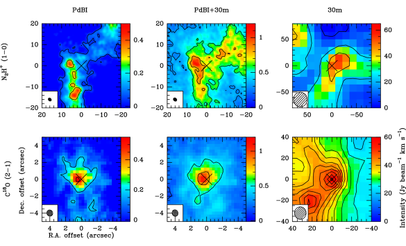
Figure 32: Same as Figure 1, but for IRAS2A. The black lines represent the integrated intensity contours of each tracer starting at 5$\sigma$ and increasing in steps of 25$\sigma$ for N₂H⁺ and 10$\sigma$ for C¹⁸O (see Tables 9 and 10.

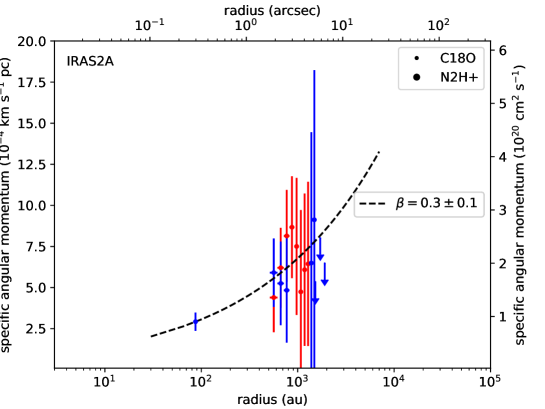
Figure 35: Same as Figure 23, but for IRAS2A.

H.5 SVS13-B

SVS13 is a multiple system located in the molecular cloud NGC1333 in the Perseus complex at a distance of (293 $\pm$ 20) pc (Ortiz-León et al. 2018). This system is composed of three main sources which are called SVS13-A, B, and C, aligned in the northeast southwest direction (Looney et al. 2003). SVS13-A is a Class I protostar and SVS13-B is a Class 0 protostar. These sources are gathered in a big filamentary structure observed at 450 $\mu$m and 1.3 mm (Chandler & Richer 2000; Hull et al. 2014). Observations at 70 $\mu$m detected SVS13-A and C but not SVS13-B, which suggests that the latter is deeply embedded in the filamentary structure (Chen et al. 2009). SVS13-A has a powerful outflow observed in the northwest southeast direction by Bachiller et al. (2000); Plunkett et al. (2013). SVS13-B also harbors a very collimated outflows (Bachiller et al. 1998). Podio & CALYPSO (in prep.) estimate the PA of the outflows at 167^∘ (see Table 2).

A velocity gradients with a magnitude of 28 km s^-1 pc^-1 and symmetric with respect to SVS13-A and B is detected in N₂H⁺ emission from PdBI observations. This gradient suggests that the binary system is physically linked (Chen et al. 2009). A study of dust continuum emission at 8 mm by Segura-Cox et al. (2016) suggests a Keplerian disk with a radius $\lesssim$25 au. A similar study from CALYPSO observations at 1.3 mm also suggests an unresolved Keplerian disk with a radius $<$60 au (Maury et al. 2019).

Figures 36 and 7 show the integrated intensity and centroid velocity maps obtained for SVS13-B from the PdBI, combined, and 30m CALYPSO datasets for the C¹⁸O and N₂H⁺ emission respectively. The C¹⁸O emission is weakly detected ($\sim$5$\sigma$) from PdBI observations for this source: the emission is dominated by its companion SVS13-A. The channel maps on Figure 37 allow us to constrain the PV_rot diagram with one point at $r\sim$100 au in the envelope (see panel (e) of Fig. 16). We observed a velocity gradient along the equatorial axis ($\mathrm{v}-\mathrm{v}_{\mathrm{sys}}<$0.4 km s^-1, see panel (e) of Fig. 16) in the combined velocity maps of the C¹⁸O emission ($r<$500 au). From the PdBI and combined velocity maps in N₂H⁺ emission (see top left and middle panels on Figure 7), the velocity gradient is dominated by the intrinsic velocity of the protostar SVS13-A. At larger scales ($r>$4500 au), the velocity gradients have an angle difference $\Delta\Theta\geq$70^∘ with respect to the equatorial axis (see Table 2). These gradients are not due to rotational motions of the envelope but motions from larger scales. Moreover, the integrated intensity trace a filamentary structure which are consistent with the filament in which the source is embedded (see right panels on Figure 7).

The panel (e) of Fig. 16 shows the PV_rot diagram of SVS13-B built from the velocity gradients observed in C¹⁸O emission at scales of $r<$500 au. The index of the fitting by a power-law ($\alpha\sim$-0.9, see Table 3) is consistent with an infalling and rotating envelope. Figure 39 shows the radial distribution of the specific angular momentum of SVS13-B at radii of 100$-$500 au.

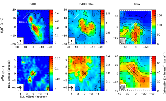
Figure 36: Same as Figure 1, but for SVS13-B. The white cross represents the position of the Class I protostar SVS13-A determined from the 1.3 mm dust continuum emission (Maury et al. 2019). The black lines represent the integrated intensity contours of each tracer starting at 5$\sigma$ and increasing in steps of 40$\sigma$ for N₂H⁺ and 10$\sigma$ for C¹⁸O (see Tables 9 and 10.

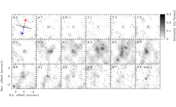
Figure 37: Same as Figure 22, but for SVS13-B. The systemic velocity is estimated to be $\mathrm{v}_{\mathrm{sys}}=$8.3 km s^-1 (see Table 15).

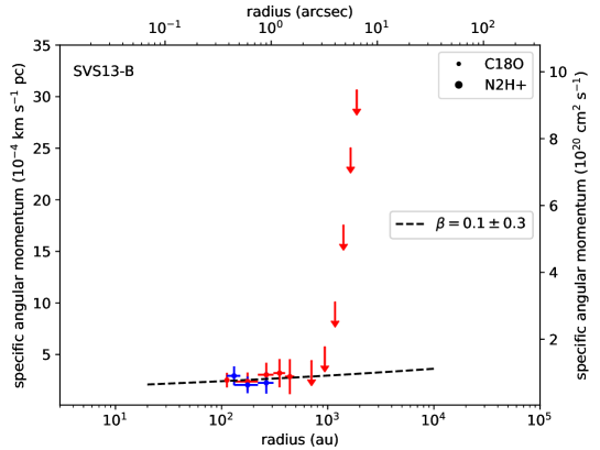
Figure 39: Same as Figure 23, but for SVS13-B.

H.6 IRAS4A

The class 0 protostar IRAS4A is located in the molecular cloud NGC1333 in the Perseus complex at (293 $\pm$ 20) pc (Ortiz-León et al. 2018), in the vicinity of another young multiple system, IRAS4B (Lay et al. 1995). It harbors a $\sim$2^′′ binary system (Looney et al. 2000; Girart et al. 2006; Jørgensen et al. 2007; López-Sepulcre et al. 2017; Maury et al. 2019) and the dust continuum emission at (sub)millimeter wavelengths is dominated by the main protostar IRAS4A1. Santangelo et al. (2015) and Podio & CALYPSO (in prep.) estimate the PA of the outflows at 180^∘ (see Table 2).

Figure 41 shows the integrated intensity obtained for IRAS4A from the PdBI, combined, and 30m CALYPSO datasets for the C¹⁸O and N₂H⁺ emission respectively. C¹⁸O emission from the PdBI dataset is centered on the main protostar IRAS4A1 (RA: 03^h29^m10^s.537, Dec.: 31^∘13$\arcmin$30^′′.98; see Table 2 and Figure 41). This is why, the origin of the coordinate offsets is chosen to be the main protostar to study the kinematics in the protostellar envelope of IRAS4A. We also noticed a hole in the integrated intensity and column density (see Figure 40) that suggests the C¹⁸O emission may be optically thick at scales of $r\lesssim$100 au.

Belloche et al. (2006) find two velocity components at $r\sim$6000 au by analyzing CS, C₃₄S and, N₂H⁺ lines obtained with the 30m. This suggests that IRAS4A is collapsing with a velocity of $\mathrm{v}<$ 7.30 km s^-1 triggered by a fast external compression with a velocity of $\mathrm{v}>$ 7.30 km s^-1. Figures 7 show the centroid velocity maps obtained for SVS13-B from the PdBI, combined, and 30m CALYPSO datasets for the C¹⁸O and N₂H⁺ emission respectively. To minimize contamination by external cloud compression, the velocity maps were constructed by fitting and removing a second gaussian component fixed at 7.7 km s^-1.

The gradients observed in the PdBI and combined velocity maps of the C¹⁸O emission (see bottom left and middle panels on Figure 8) have an angle difference of $\Delta\Theta\leq$11^∘ with respect to the equatorial axis (see Table 2). These gradients are consistent with those observed in C¹⁷O emission from SMA observations (Ching et al. 2016). We notice that the gradient is aligned along and symmetric with respect to the binary system IRAS4A1 and IRAS4A2. This could suggest that the binary system is physically linked by orbital motions.

The channel maps do not exhibit an organized spatial distribution of velocities along the equatorial axis : the central emission fit show a position angle $>$—45${}^{\circ}|$ with respect to the equatorial axis, suggesting a possible contamination by the outflow kinematics (see Figure 42). To minimize this contamination and probe rotational motions in the equatorial axis, we used the method in the image plane in the PdBI dataset instead of working in the visibilities to constrain in the inner envelope (200$-$800 au).

The velocity gradients observed in the PdBI velocity maps of the N₂H⁺ emission (see top left panels on Figure 8) have a direction of $\Theta\sim$-69^∘ consistent with the equatorial axis. However, at larger scales ($r>$1000 au), the N₂H⁺ emission is dominated by external cloud compression. The gradient have a direction of $\Theta\geq$32^∘. Moreover, the integrated intensity of N₂H⁺ emission from the 30m datasets (see right top panel on Figure 41) trace the filamentary structure which are consistent with the filament in which the source is embedded.

The panel (l) of Fig. 16 shows the PV_rot diagram of IRAS4A built from the velocity gradients observed at scales of $r<$1600 au. This is the only source with increasing velocities from small to large scales. The index of the fitting by a power-law ($\alpha\sim$0.8, see Table 3) could be interpreted by solid-body rotation, but as the velocity gradient is not uniform as expected, this is not a robust interpretation for this source (see Sect. 5.1). Moreover, by considering only point at $r<$550 au, the index of the fitting by a power-law is consistent with an infalling and rotating envelope ($\alpha\sim$-1.3, see Table 3). We did not take this source into account to build the radial distribution of the specific angular momentum due to rotation motions.

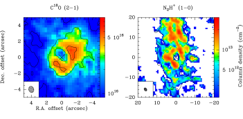
Figure 40: Same Figure as 21 for IRAS4A. The N₂H⁺ (1$-$0) column density maps is determined from the PdBI datasets. The integrated intensity overlaid in black solid line is the integrated intensity from the 7 hyperfine components of the transition (see top left panel on Figure 41).

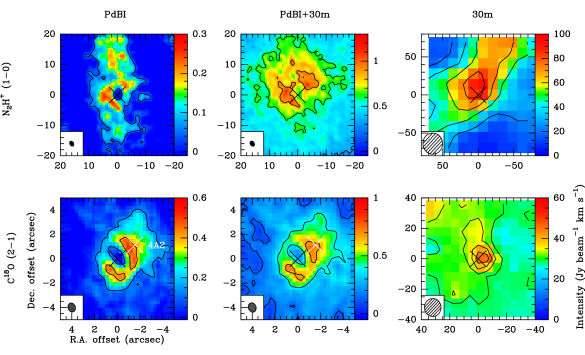
Figure 41: Same as Figure 1, but for IRAS4A. The white cross represents the position of secondary protostar IRAS4A2 determined from the 1.3 mm dust continuum emission (see Table 2). The black cross represents the position of the main protostar IRAS4A1 of the multiple system. The black lines represent the integrated intensity contours of each tracer starting at 5$\sigma$ and increasing in steps of 30$\sigma$ for N₂H⁺ and 10$\sigma$ for C¹⁸O (see Tables 9 and 10.

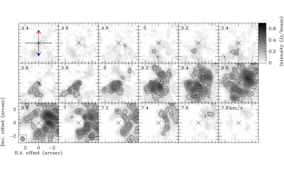
Figure 42: Same as Figure 22, but for IRAS4A. The systemic velocity is estimated to be $\mathrm{v}_{\mathrm{sys}}=$6.6 km s^-1 (see Table 15).

H.7 IRAS4B

IRAS4B (or NGC1333-IRAS4B) is a Class 0 protobinary system in the Perseus molecular cloud at a distance of (293 $\pm$ 20) pc (Ortiz-León et al. 2018). The binary companions 4B1 and 4B2 are separated by $\sim$11^′′ (Looney et al. 2000; Jørgensen et al. 2007). The source harbors a young bipolar outflow almost aligned along a north-south direction (Choi 2001). Podio & CALYPSO (in prep.) distinguish two outflows: a first associated with the main protostar 4B1 at 167^∘ and a second with a PA of -99^∘ (see Table 2). IRAS4B is in the vicinity of IRAS4A which undergo a collapse triggered by a fast external compression with a velocity of $\mathrm{v}>$ 7.30 km s^-1 (Belloche et al. 2006). Thus, collapse of IRAS4B could have triggered in the same way. It is why, to minimize contamination by external cloud compression, the velocity maps were constructed by fitting and removing a second Gaussian component fixed at 7.7 km s^-1 (see Figure 43). Previous studies of C¹⁸O (2$-$1) emission from SMA observations are detected no organized velocity gradients consistent with rotational motions (Yen et al. 2013, 2015b).

Figure 9 shows the centroid velocity maps obtained for IRAS4B from the PdBI, combined, and 30m CALYPSO datasets for the C¹⁸O and N₂H⁺ emission. The gradients observed in the PdBI and combined velocity maps of the C¹⁸O emission (see bottom left and middle panels on Figure 9) have an angle difference of $\Delta\Theta\leq$20^∘ with respect to the equatorial axis (see Table 2). The velocity gradients observed in the PdBI velocity maps of the N₂H⁺ emission (see top left panels on Figure 9) is also consistent with the equatorial axis.

However, the channel maps do not exhibit an organized spatial distribution of velocities along the equatorial axis : the central emission fit show a position angle $>$—45${}^{\circ}|$ with respect to the equatorial axis, suggesting a possible contamination by the outflow kinematics (see Figure 44). To minimize this contamination and probe rotational motions in the equatorial axis, we used the method in the image plane in the PdBI dataset instead of working in the visibilities to constrain in the inner envelope (200$-$500 au).

At outer envelope scales ($r>$1000 au), the N₂H⁺ emission shows a reversed gradient dominated by external cloud compression. Moreover, the integrated intensity of N₂H⁺ emission from the 30m datasets (see right top panel on Figure 43) trace the a filamentary structure which are consistent with the filament in which the source is embedded.

The panel (g) of Fig. 16 shows the PV_rot diagram of IRAS4B built from the velocity gradients observed at scales of $r<$1100 au. The index of the fitting by a power-law ($\alpha\sim$-0.6, see Table 3) is consistent with a Keplerian rotation. However, we also obtain a good reduced $\chi^{2}$ when we fit the PV_rot diagram by an infalling and rotating envelope by fixing the index of the power-law at -1 ($\sim$0.6, see Table 3). Thus, for this source, the CALYPSO dataset only allow us to estimate a range of the power-law index between -1 and -0.6 (see Table 3) at the scales of 170$-$1100 au probed in our analysis. Moreover, Keplerian rotation is not detected at the smaller envelope radii investigated by Maret et al. (2020). Thus, the Keplerian rotation due to a large disk is not a robust interpretation for this source. Figure 46 shows the radial distribution of the specific angular momentum of IRAS4B at radii of 170$-$1100 au.

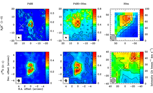
Figure 43: Same as Figure 1, but for IRAS4B. The white crosses represent the position of secondary protostar IRAS4B2 and the position of IRAS4A, respectively, determined from the 1.3 mm dust continuum emission (see Table 2). The black cross represents the position of the secondary protostar L1448-NB2 of the multiple system. The black lines represent the integrated intensity contours of each tracer starting at 5$\sigma$ and increasing in steps of 25$\sigma$ for N₂H⁺ and 10$\sigma$ for C¹⁸O (see Tables 9 and 10.

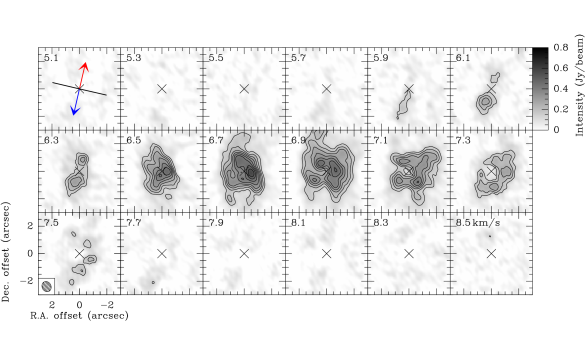
Figure 44: Same as Figure 22, but for IRAS4B. The systemic velocity is estimated to be $\mathrm{v}_{\mathrm{sys}}=$6.9 km s^-1 (see Table 15).

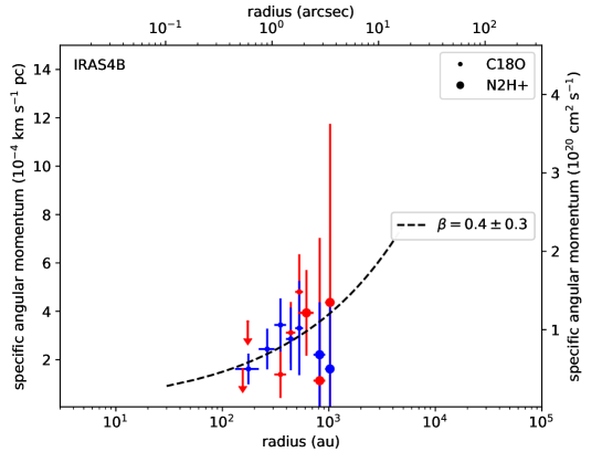
Figure 46: Same as Figure 23, but for IRAS4B.

H.8 IRAM04191

At a distance of 140 pc (Torres et al. 2009), IRAM04191+1522 (hereafter IRAM04191) is located in the southern part of the Taurus cloud in the viciny of the Class I protostar IRAS04191. Its envelope mass (0.5 M_⊙, André et al. 2000), its low luminosity (0.1 L_⊙, Dunham et al. 2006), and its temperature suggest that is one of the youngest accreting and isolated Class 0 sources known in Taurus ($t\sim$1$-$3 $\times$ 10⁴ yr, André et al. 1999). This source harbors a strongly collimated outflow with a PA=28^∘ (Belloche et al. 2002) and an inclination angle to the line of sight estimated at $\sim$40^∘ (André et al. 1999; Maret et al. 2014). A new study by Podio & CALYPSO (in prep.) estimates the PA of the outflows at 20^∘ (see Table 2). We used this later value for our study. From CALYPSO observations, Maury et al. (2019) estimate an envelope mass of 0.45 M_⊙ and did not resolve candidate disk down to $<$50 au.

The 30m observations of several molecular lines suggests signatures of the envelope infalling motions with an estimated velocity of $\sim$0.2 km s^-1 to $r\sim$1000 au and $\sim$0.1 km s^-1 to $r\sim$10000 au (Belloche et al. 2002). These observations associated with radiative transfer model allowed kinematics of the outer envelope to be constrained. A strong velocity gradient of $\sim$40 km s^-1 pc^-1 was detected at scales of $\sim$3500 au along the northwest-southeast direction, namely in the equatorial axis. At $\sim$1500 au, Lee et al. (2005) detect a velocity gradient of $\sim$100 km s^-1 pc^-1. These gradient are interpreted as rotational motions of the protostellar envelope (Belloche et al. 2002; Takakuwa et al. 2003).

Figures 47 and 10 show the integrated intensity and centroid velocity maps obtained for IRAM04191 from the PdBI, combined, and 30m CALYPSO datasets for the C¹⁸O and N₂H⁺ emission, respectively. The C¹⁸O emission is weakly detected ($\sim$5$\sigma$) from PdBI observations for this source which is one of the lowest luminosity sources in our sample (see bottom left panel on Figure 10). However, the combined map allows the kinematics of the protostellar envelope between 50 and 1000 au to be constrained. At those scales (see bottom middle panel on Figure 10), we noticed a velocity gradients with a direction of $\Theta$= -83^∘, consistent with the equatorial axis. At $r>$1000 au, the velocity gradients observed in the velocity maps of the N₂H⁺ emission (see top panels on Figure 10) have a direction of$\Theta\sim$100^∘, consistent with those detected by Belloche et al. (2002) at similar scales. Therefore, there is a reversal of the kinematics between inner ($\sim$500 au) and outer envelope scales ($>$1000 au).

The panel (h) of Fig. 16 shows the PV_rot diagram of IRAM04191 built from the velocity gradients observed at scales of 50$-$800 au. The index of the fitting by a power-law ($\alpha\sim$-0.3, see Table 3) is consistent with a Keplerian rotation. However, we also obtain a good reduced $\chi^{2}$ when we fit the PV_rot diagram by an infalling and rotating envelope by fixing the index of the power-law at -1 ($\sim$1.1, see Table 3). Thus, for this source, the CALYPSO dataset only allow us to estimate a range of the power-law index between -1 and -0.3 (see Table 3) at the scales of 50$-$800 au probed in our analysis. Moreover, Keplerian rotation is not detected at the smaller envelope radii investigated by Maret et al. (2020). Thus, the Keplerian rotation due to a large disk is not a robust interpretation for this source. Figure 50 shows the radial distribution of the specific angular momentum of IRAM04191 at radii of 50$-$800 au.

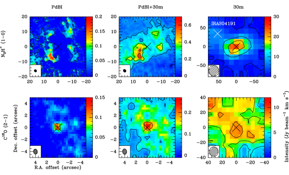
Figure 47: Same as Figure 1, but for IRAM04191. The white cross represents the position of the Class I protostar IRAS04191. The black cross represents the position of IRAM04191 determined from the 1.3 mm dust continuum emission (see Table 2). The black lines represent the integrated intensity contours of each tracer starting at 5$\sigma$ and increasing in steps of 30$\sigma$ for N₂H⁺ and 6$\sigma$ for C¹⁸O (see Tables 9 and 10).

Figure 49: Same Figure as 21 for IRAM04191.

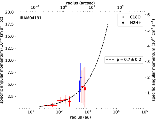
Figure 50: Same as Figure 23, but for IRAM04191.

H.9 L1521F

At a distance of 140 pc (Torres et al. 2009), L1521F (or MC27) is one of the densest cores in Taurus cloud. This source was firstly identified as a starless core (Codella et al. 1997; Onishi et al. 1999; Crapsi et al. 2004). Its very low luminosity (L¡0.004; Maury et al. 2019) indicates that it is among the youngest known Class 0 protostars (André et al. 2000) and still may preserve the initial conditions of star formation (Terebey et al. 2009). The emission of the molecular line HCO⁺ showing a high central density and an asymmetric signature typical of the collapse suggests that the source is in the early stages of gravitational collapse (Onishi et al. 1999). Its low luminosity of $L_{\mathrm{bol}}<$0.04 (Maury et al. 2019; Ladjelate et al. in prep.) indicating that is one of the known Class 0 youngest prostars (André et al. 2000), L1521F could still preserve its initial conditions (Bourke et al. 2006; Terebey et al. 2009). N₂H⁺ and NH₃ emissions from VLA observations show a flattened structure perpendicular to the outflows (Tobin et al. 2010). Podio & CALYPSO (in prep.) do not detect clear jet signature in SiO and SO but only blue and red-shifted clumps in CO. In our study of the kinematics, we used the PA of the outflows at 240^∘ observed in CO and HCO⁺ by Tokuda et al. (2014, 2016) (see Table 2). Recent ALMA observations of ¹²CO emission showed a clear velocity gradient in the equatorial axis consistent with the presence of a disk of radius of $\sim$10 au surrounded a stellar embryo of $\sim$0.2 $M_{\odot}$ (Tokuda et al. 2017).

Figure 51 shows the integrated intensity maps obtained for L1521F from the PdBI, combined, and 30m CALYPSO datasets for the C¹⁸O and N₂H⁺ emission. The C¹⁸O emission is weakly detected ($\sim$5$\sigma$) from the PdBI observations for this source which is one of the lowest luminosity sources in our sample (see bottom left panel on Figure 11). The emission peak does not correspond to the continuum emission peak at 1.3 mm determined from the PdBI dataset by Maury et al. (2019) (see Table 2). This is consistent with the existence of a starless high-density core, MMS-2 (RA:4^h28^m38^s.89, Dec.:+26^∘51$\arcmin$33^′′.9) detected by ALMA Cycle 0 observations in dust continuum and H¹³CO(3–2) emissions (Tokuda et al. 2014). The protostar MMS-1 (RA:4^h28^m38^s.96, Dec.: +26^∘51$\arcmin$35^′′) is also not spatially resolved in H¹³CO(3–2) emission. The L1521F protostar is not spatially resolved by the emission H¹³CO (3$-$2) but a clear velocity gradient is observed along the northwest southeast axis at outer envelope scales consistent with the equatorial axis (Tokuda et al. 2014). This velocity gradient is in the same direction as the elongated structure we observed in combined N₂H⁺ emission (see top middle panel on Figure 11) and also observed by Tobin et al. (2010). The absence of velocity gradient at small scales ($r<$1500 au) is interpreted as due to low dust temperature of $T\sim$10K (Tokuda et al. 2014, 2016) which is not sufficient to excite high density molecules ($E_{\mathrm{upper}}$=15.8 K for the molecular transition C¹⁸O (2$-$1); CDMS).

Figures 11 show the centroid velocity maps obtained for L1521F from the PdBI, combined, and 30m CALYPSO datasets for the C¹⁸O and N₂H⁺ emission. Only the 30m velocity map of the C¹⁸O emission (see bottom right panel on Figure 11) shows a gradient with a blue- and a red-shifted velocity components along the equatorial axis at radii $\sim$3000 au. The direction of this gradient ($\Theta\sim$ -8^∘) is consistent with the equatorial axis axis and the gradients previously observed by Tokuda et al. (2014). However, we noted that the integrated intensity of the C¹⁸O emission from the 30m datasets does not trace the envelope but a more complex and diffuse structure.

The panel (i) of Fig. 16 shows the PV_rot diagram of L1521F built from the velocity gradients observed at scales of 1500$-$4200 au. The index of the fitting by a power-law is close to 0 (see Table 3). However, we also obtain a quite good reduced $\chi^{2}$ when we fit the PV_rot diagram by an infalling and rotating envelope by fixing the index of the power-law at -1 ($\sim$1, see Table 3). Thus, for this source, the CALYPSO dataset only allow us to estimate a range of the power-law index between -1 and 0 (see Table 3) at the scales of 1500$-$4200 au probed in our analysis. Figure 54 shows the radial distribution of the specific angular momentum of L1521F at radii of 1500$-$4200 au.

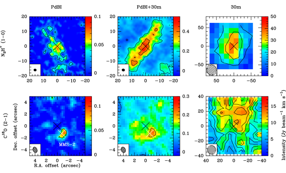
Figure 51: Same as Figure 1, but for L1521F. The white cross represents the position of the starless dense core MMS-2. The black lines represent the integrated intensity contours of each tracer starting at 5$\sigma$ and increasing in steps of 30$\sigma$ for N₂H⁺ and 10$\sigma$ for C¹⁸O (see Tables 9 and 10.

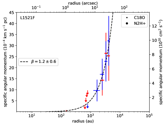
Figure 54: Same as Figure 23, but for L1521F.

H.10 L1527

At a distance of 140 pc (Torres et al. 2009) in the Taurus molecular cloud, L1527 is the closest Class 0/I source which exhibits a candidate proto-planetary disk with an outer radius of 50$-$90 au around a 0.2$-$0.3 M_⊙ central object (Tobin et al. 2012; Ohashi et al. 2014). A recent study by Aso et al. (2017) find an outer radius of 74 au and a central mass of 0.45 M_⊙. The embryo mass is close of the envelope mass ($\sim$1 M_⊙), which sets the source at the boundary between the phases Class 0 and Class I. This source is an ideal target for studying the kinematics of the disk and the envelope at high angular resolution because it is seen almost edge-on, with an angle $\sim$90^∘ with respect to the sky plane (Ohashi et al. 1997b). L1527 would also be embedded in a filament with an angle of PA$\sim$135^∘ (Marsch & HGBS, in prep).

Figures 55 and 12 show the integrated intensity and centroid velocity maps obtained for L1527 from the PdBI, combined, and 30m CALYPSO datasets for the C¹⁸O and N₂H⁺ emission, respectively. At scales of $r<$2000 au (see left and middle panels on Figure 12), show a clear velocity gradient along the north-south axis. These velocity gradients are consistent with those observed in C¹⁸O (2$-$1) emission with CARMA, SMA and ALMA (Tobin et al. 2012; Yen et al. 2013, 2015b; Ohashi et al. 2014). The linear gradient fits give orientations of -9^∘ $<\Theta<$26^∘ which is consistent with the equatorial axis direction assumed perpendicular to the outflows (see Table 2). Velocity maps from the 30m datasets at scales $\sim$3000$-$5000 au (see right panels on Figure 12) show gradients along the east-west axis opposite to the outflow direction, with an orientation $\sim$113$-$123^∘ (see Table 2).

The panel (j) of Fig. 16 shows the PV_rot diagram of L1527 built from the velocity gradients observed at scales of $r<$2000 au. The index of the fitting by a power-law is consistent with a rotating and infalling envelope ($\alpha\sim$-1.1, see Table 3). This result is consistent with previous studies of Yen et al. (2013) and Ohashi et al. (2014) which are found indices of $\sim$-1 and $\sim$-1.2 on scales of 40$-$500 au and 100$-$1500 au, respectively. Ohashi et al. (2014) constrain the specific angular momentum at $j\sim$6 $\times$10^-4 km s^-1 pc at radii of 100$-$1600 au. This value is consistent with the value we found on the Fig. 58 which shows the radial distribution of the specific angular momentum of L1527 at radii of 40$-$2000 au.

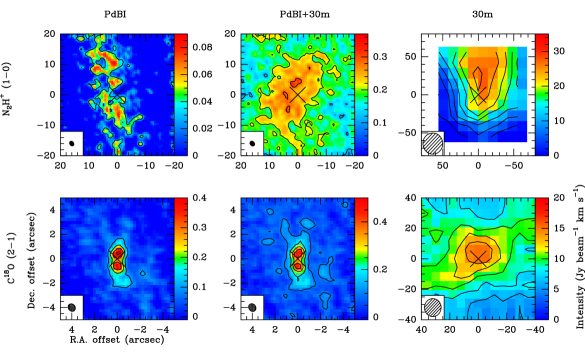
Figure 55: Same as Figure 1, but for L1527. The black lines represent the integrated intensity contours of each tracer starting at 5$\sigma$ and increasing in steps of 13$\sigma$ for N₂H⁺ and 5$\sigma$ for C¹⁸O (see Tables 9 and 10.

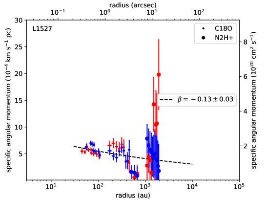
Figure 58: Same as Figure 23, but for L1527.

H.11 L1157

In the Cepheus molecular cloud at a distance previously estimated to be 250 pc (Looney et al. 2007) but determined at (352 $\pm$ 18) pc by recent Gaia parallax measurements (Zucker et al. 2019), L1157 is a Class 0 protostar deeply embedded within a large circumstellar envelope (Gueth et al. 2003; Beltrán et al. 2004). The source harbors a powerful asymmetrical bipolar outflows at large scales (Tafalla & Bachiller 1995; Zhang et al. 1995; Gueth et al. 1996). Podio et al. (2016) and Podio & CALYPSO (in prep.) estimate the PA of the outflows at 163^∘ (see Table 2). Previous study of C¹⁸O (2$-$1) observations with SMA showed no clear sign of rotational motions but kinematic models predict L1157 exhibit a possible disk with an outer radius $<$5 au (Yen et al. 2015b).

Figures 59 and 13 show the integrated intensity and centroid velocity maps obtained for L1157 from the PdBI, combined, and 30m CALYPSO datasets for the C¹⁸O and N₂H⁺ emission, respectively. Velocity maps of C¹⁸O emission from the PdBI and combined datasets (see bottom left and middle panels on Figure 13) show gradients with a direction of $\Theta\sim$13$-$35^∘ (see Table 2). They are dominated by the kinematics of the outflows but a weak velocity gradient is observed along the equatorial axis at radii $r<$2000 au. Velocity maps of N₂H⁺ emission from PdBI and combined datasets (see top left and middle panels on Figure 13) trace cavities along the outflow axis. These gradients are consistent with those detected in CARMA observations by Chiang et al. (2010) and Tobin et al. (2011). At scales of $r>$2500 au, velocity maps from the 30m datasets (right panels on Figure 13) show a gradient with a direction of $\Theta\sim$ -130^∘, in the opposite direction with respect to small scales observed along the equatorial axis.

The panel (k) of Fig. 16 shows the PV_rot diagram of L1157 built from the velocity gradients observed at scales of $r<$700 au. The index of the fitting by a power-law is close to 0 (see Table 3), consistent with differential rotation of the envelope. At each PdBI emission channel, the central emission fit show a position angle $>$—45${}^{\circ}|$ with respect to the equatorial axis, suggesting a contamination by the outflow kinematics (see Figure 60). To minimize this contamination and probe rotational motions in the equatorial axis, we used the method in the image plane in the PdBI dataset instead of working in the visibilities to constrain in the inner envelope (80$-$200 au). Figure 62 shows the radial distribution of the specific angular momentum of L1157 at radii of 80$-$700 au.

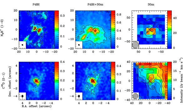
Figure 59: Same as Figure 1, but for L1157. The black lines represent the integrated intensity contours of each tracer starting at 5$\sigma$ and increasing in steps of 25$\sigma$ for N₂H⁺ and 10$\sigma$ for C¹⁸O (see Tables 9 and 10.

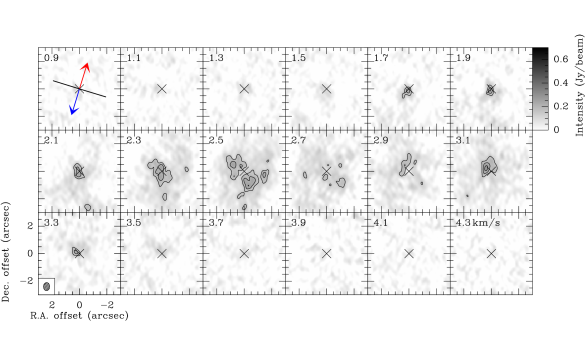
Figure 60: Same as Figure 22, but for L1157. The systemic velocity is estimated to be $\mathrm{v}_{\mathrm{sys}}=$2.65 km s^-1 (see Table 15).

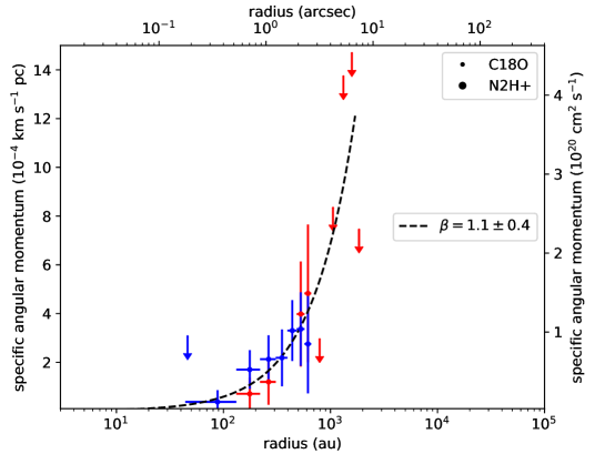
Figure 62: Same as Figure 23, but for L1157.

H.12 GF9-2

GF9-2 (L1082C Benson & Myers 1989 or GF9-Core Ciardi et al. 2000) is located in the filamentary cloud GF9-2 (or LDN 1082) at a distance of 200 pc (Wiesemeyer 1997; Wiesemeyer et al. 1998). In this study, we adopt this distance but it is very uncertain and some studies estimated a higher distance between 440$-$470 pc (Viotti 1969, C. Zucker, priv. comm.) and 900 pc (Reid et al. 2016). Due to its low luminosity (0.3 L_⊙, Wiesemeyer 1997), GF9-2 is has been cataloged as a transitional object between the prestellar and the Class 0 phases (Wiesemeyer et al. 1999). GF9-2 would be the youngest source in our sample and would therefore retain the initial conditions of its gravitational collapse because the central embryo does not have a powerful bipolar flow (Furuya et al. 2006). Podio & CALYPSO (in prep.) detect for the first time the outflows with a PA of 0^∘ (see Table 2).

Figures 63 and 14 show the integrated intensity and centroid velocity maps obtained for GF9-2 from the PdBI, combined, and 30m CALYPSO datasets for the C¹⁸O and N₂H⁺ emission, respectively. The CALYPSO datasets allow us to constrain the kinematics of this source at the envelope scales for the first time. Only the PdBI and combined maps of the C¹⁸O emission (see bottom left and middle panels on Figure 14) show a velocity gradient associated with the source. The gradient is consistent with the equatorial axis, with a direction of -160${}^{\circ}<\Theta<$-130^∘ (see Table 2). Moreover, the N₂H⁺ integrated intensity from the 30m datasets at scales of $r>$3000 au traces the filament structure in which the source is embedded.

The panel (l) of Fig. 16 shows the PV_rot diagram of GF9-2 built from the velocity gradients observed at scales of $r<$900 au. The index of the fitting by a power-law is consistent with an infalling and rotating envelope ($\sim$-0.8, see Table 3). Figure 66 shows the radial distribution of the specific angular momentum of GF9-2 at radii of 70$-$900 au.

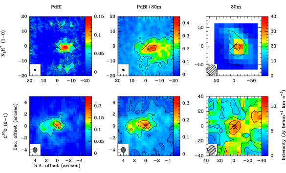
Figure 63: Same as Figure 1, but for GF9-2. The black lines represent the integrated intensity contours of each tracer starting at 5$\sigma$ and increasing in steps of 25$\sigma$ for N₂H⁺ and 5$\sigma$ for C¹⁸O (see Tables 9 and 10.

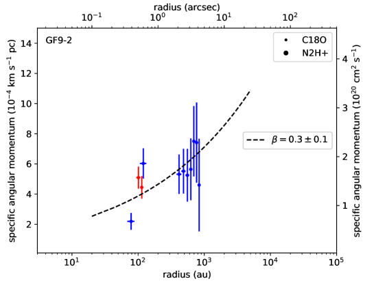
Figure 66: Same as Figure 23, but for GF9-2.