BLUE: combining correlated estimates of physics observables within ROOT using the Best Linear Unbiased Estimate method

Abstract

This software performs the combination of $m$ correlated estimates of $n$ physics observables ($m\geq n$) using the Best Linear Unbiased Estimate (BLUE) method. It is implemented as a C++ class, to be used within the ROOT analysis package. It features easy disabling of specific estimates or uncertainty sources, the investigation of different correlation assumptions, and allows performing combinations according to the importance of the estimates. This enables systematic investigations of the combination on details of the measurements from within the software, without touching the input.

Code metadata
Current code version	2.4.0
Permanent link to code/repository used	https://github.com/ElsevierSoftwareX/SOFTX_2020_16
for this code version	https://blue.hepforge.org
Code Ocean compute capsule
Legal Code License	LGPL
Code versioning system used	none
Software code languages, tools, and services used	C++
Compilation requirements, operating environments & dependencies	depends on https://root.cern.ch
If available Link to developer documentation/manual	https://blue.hepforge.org
Support email for questions	Richard.Nisius@mpp.mpg.de

1 Motivation and significance

The combination of a number of correlated estimates for a single observable is discussed in Ref. [1]. Here, the term estimate denotes a particular outcome (measurement) of an experiment based on an experimental estimator (an algorithm for a measurement) of the observable, which follows a probability density function (PDF). The particular estimate obtained by the experiment may be a likely or unlikely outcome for that PDF. Repeating the measurement numerous times under identical conditions, the estimates will follow the underlying PDF of the estimator.

The metadata for the BLUE software are listed in the Code metadata table. The software uses the Gaussian approximation for the uncertainties and performs a $\chi^{2}$ minimization to obtain the combined value. In Ref. [1], this minimization is expressed using the mathematically equivalent BLUE ansatz. Provided the estimators are unbiased, when applying this formalism the Best Linear Unbiased Estimate of the observable is obtained with the following meaning: Best: the combined result for the observable obtained this way has the smallest variance; Linear: the result is constructed as a linear combination of the individual estimates; Unbiased Estimate: when the procedure is repeated for a large number of cases consistent with the underlying multi-dimensional PDF, the mean of all combined results equals the true value of the observable. The formulas for more than one observable [2] are implemented in the BLUE software, which is programmed as a separate class of the ROOT analysis framework [3].

The easiest case of two correlated estimates of the same observable is briefly illustrated here. Already for this case, the main features of the combination can easily be understood. For further information and the derivation of the formulas the reader is refereed to Ref. [4]. Let $x_{\mathrm{1}}$ and $x_{\mathrm{2}}$ with variances $\sigma_{1}^{2}$ and $\sigma_{2}^{2}$ be two estimates from two unbiased estimators $X_{\mathrm{1}}$ and $X_{\mathrm{2}}$ of the true value $x_{\mathrm{T}}$ of the observable and $\rho$ the total correlation of the two estimators. Without loss of generality it is assumed that the estimate $x_{\mathrm{1}}$ stems from an estimator $X_{\mathrm{1}}$ of $x_{\mathrm{T}}$ that is at least as precise as the estimator $X_{\mathrm{2}}$ yielding the estimate $x_{\mathrm{2}}$, such that $z\equiv\sigma_{2}/\sigma_{1}\geq 1$. In this situation the BLUE $x$ of $x_{\mathrm{T}}$ is:

$$x =\, (1-\beta)\,x_{\mathrm{1}}+\beta\,x_{\mathrm{2}}\,$$

where $\beta$ is the weight of the less precise estimate and the sum of weights is unity by construction. The variable $x$ is the combined result and $\sigma_{x}^{2}$ is its variance, i.e. the uncertainty assigned to the combined value is $\sigma_{x}$. For a number of $z$ values the two quantities $\beta$ and $\sigma_{x}$/$\sigma_{1}$ as functions of $\rho$ are shown in Fig. 1. Their functional forms are also written in the figures. The functions are valid for $-1\leq\rho\leq 1$ and $z\geq 1$, except for $\rho=z=1$.

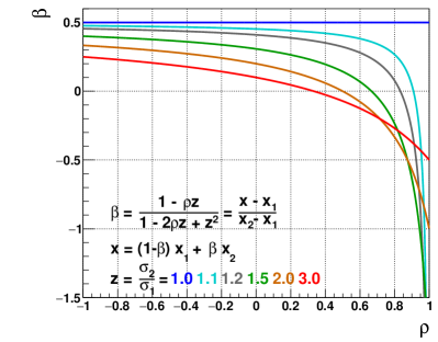
(a) $\beta$ as a function of $\rho$

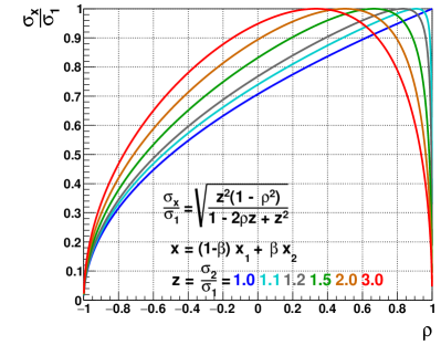
(b) $\sigma_{x}$/$\sigma_{1}$ as a function of $\rho$

Figure 1: The variables $\beta$ (a) and $\sigma_{x}$/$\sigma_{1}$ (b) shown as functions of $\rho$ for a number of $z$ values.

Fig. 1 displays the strong dependence of the uncertainty in the combined value on $z$ and $\rho$. For the special situation of $\rho=1/z$ the uncertainty $\sigma_{x}$ equals $\sigma_{1}$, i.e. the precision in the observable is not improved by adding the second measurement. For $\rho=\pm 1$ the uncertainty in the combined result vanishes, i.e. $\sigma_{x}=0$, a mere consequence of the conditional probability for $X_{\mathrm{2}}$ given the measured value of $x_{\mathrm{1}}$, see Ref. [4] for details. It is worth noticing that in most regions of the ($\rho$, $z$)-plane the sensitivity of $\sigma_{x}$/$\sigma_{1}$ to $\rho$ is stronger than to $z$. This means, reducing the correlation of the estimates in most cases gives a larger improvement in precision in the combined value than reducing $z$.

2 Software description

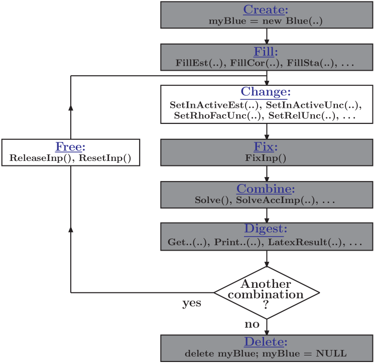
Figure 2: Flowchart of the BLUE software. The gray boxes display the steps to be performed for a single combination with unchanged inputs. The white boxes display the optional steps for further combinations with changed inputs and/or different solving methods. In each rectangular box, the first line indicates the performed action, while the following line(s) list the functions to use.

To use the BLUE combination software, a working installation of the ROOT package [3] is needed. The software allows repeated combinations interleaved with an arbitrary number of changes to various aspects of the input, achieved using Set…() functions. In addition, it gives access to many intermediate quantities used in the combination via Get…() and Print…() functions. Only at well-defined steps of the computation, will the returned quantities be meaningful. To enable the above flexibility, the BLUE object has several states like IsFilledInp, IsFixed or IsSolved that can be false or true. The various functions are only enabled, if the object has the appropriate state.

The mandatory inputs to the software are the measured values, their uncertainties for the various statistical and systematic effects relevant to the measurements, and the estimator correlations for each of those uncertainties. Those are inserted into the BLUE object by means of the filling functions FillEst() and FillCor(). The end of filling the mandatory inputs is automatically recognized by the software. At this point, the initial input is saved, auxiliary information is calculated, IsFilledInp is set to true and all filling functions are disabled. Consequently, the optional additional input like names, print formats and a logo, all have to be filled before the end of filling the mandatory input is reached.

The most important object states can be controlled by function calls. For example, a call to FixInp() initiates the calculation of various quantities and sets IsFixed to true, thereby enabling the use of a number of Get…() and Print…() functions. A subsequent call to any of the solving methods Solve…() performs the desired combination, and finally sets IsSolved to true. In this scheme, solving is only possible after a call to FixInp(), and changing the inputs only after a call to ReleaseInp() or ResetInp(). Internally, the combination is always performed on a temporary copy of the initial input, which can be successively altered using the sequence of calling ReleaseInp(), Set…() and FixInp(). Since the initial input was saved as described above, a call to ResetInp() allows to return to this situation.

2.1 Combination workflow

The flowchart of the software is shown in Fig. 2. After calling the constructor of the class ($\mathtt{\underline{Create}:}$), thereby defining the number of estimates, uncertainties and observables, the measurements together with their uncertainties and correlations are passed to the software ($\mathtt{\underline{Fill}:}$). If wanted, the inputs can be adapted ($\mathtt{\underline{Change}:}$). Combinations are performed following the loop of fixing ($\mathtt{\underline{Fix}:}$), combining ($\mathtt{\underline{Combine}:}$) and evaluating the result ($\mathtt{\underline{Digest}:}$). Before changing the inputs for the next combination, they have to be freed ($\mathtt{\underline{Free}:}$). For this step, two options are available, ReleaseInp() means the change proceeds from the status at the last fix, while ResetInp() reverts to the original inputs. If no further combinations are wanted, the object is deleted ($\mathtt{\underline{Delete}:}$).

2.2 Software Functionalities

One main quality of this software is the built-in flexibility for easy and thorough investigations of the impact of details of the input measurements and their correlation. With single function calls estimates or uncertainty sources can be removed from the combination, different uncertainty models (e.g. absolute or relative uncertainties) and correlation assumptions can be investigated. Another strength is the large number of different solving methods implemented, ranging from only using measurements with positive weights in the combination to a successive combination method in which the input measurements are included one at a time according to their importance, allowing an in-depth investigation of their impact on the combination.

3 Illustrative Example

	Estimates			Correlations			Result
	$M_{\mathrm{0}}$	$M_{\mathrm{1}}$	$M_{\mathrm{2}}$	$\rho_{01}$	$\rho_{02}$	$\rho_{12}$	$M$
	[GeV]	[GeV]	[GeV]				[GeV]
Value	174.86	172.63	173.25				173.92
Stat	0.35	0.54	0.24				0.20
$\mathrm{Syst}_{1}$	0.26 $\pm$ 0.06	0.66 $\pm$ 0.04	0.43 $\pm$ 0.06	$+1.00$	$+1.00$	$+1.00$	0.36
$\mathrm{Syst}_{2}$	0.09 $\pm$ 0.05	0.64 $\pm$ 0.06	0.23 $\pm$ 0.08	$+1.00$	$+1.00$	$+1.00$	0.17
$\mathrm{Syst}_{3}$	0.12 $\pm$ 0.14	0.47 $\pm$ 0.09	0.23 $\pm$ 0.11	$-1.00$	$-1.00$	$-1.00$	0.09
$\mathrm{Syst}_{4}$	0.18 $\pm$ 0.08	0.24 $\pm$ 0.05	0.10 $\pm$ 0.08	$-1.00$	$-1.00$	$-1.00$	0.02
$\mathrm{Syst}_{5}$	0.48 $\pm$ 0.09	0.53 $\pm$ 0.08	0.12 $\pm$ 0.05	$+0.50$	$+0.60$	$-0.30$	0.25
$\mathrm{Syst}$	0.59 $\pm$ 0.09	1.19 $\pm$ 0.06	0.56 $\pm$ 0.07				0.48
Total	0.69 $\pm$ 0.09	1.30 $\pm$ 0.06	0.61 $\pm$ 0.07	$+0.29$	$+0.29$	$+0.35$	0.52
$\chi^{2}$				3.00	4.28	0.25
Weight	0.42	-0.00	0.59
Pull	2.07	-1.08	-2.07

Table 1: Combination of one observable $M$ from three correlated estimates $M_{\mathrm{0}}$, $M_{\mathrm{1}}$ and $M_{\mathrm{2}}$ using the BLUE software. Counting from the left, columns 2-4 show the individual results, their uncertainties and the statistical precision in the systematic uncertainties. Columns 5-7 report the estimator correlations $\rho_{ijk}$ for the pair of estimates ($i,j$) for all sources $k$ of uncertainty. The line denoted by Total lists the total uncertainties $\sigma_{i}$ and correlations $\rho_{ij}$. The rightmost column shows the combined result. The lower part of the table reports the estimator consistencies expressed as pairwise $\chi^{2}$ values, the weights of the estimates within the combination and the pulls of the estimates. Details on the calculation of $\chi^{2}$, the weights and pulls are given in Ref. [4].

A compact example of three estimates of a single observable is listed in Table 1. The code reproducing the content of this table and all following figures is given in A. It contains detailed documentation relating the various function calls to the steps described in Fig. 2, and the obtained results to Table 1 and the respective figures. After installing the package, the only two commands to be executed from the shell prompt are:

⬇

root -b < B_SoftExample.inp > B_SoftExample.out

pdflatex B_SoftExample.tex

Although for this example the values chosen are similar to what is obtained in measurements of the top quark mass, this example is purely artificial. The estimate $M_{\mathrm{0}}$ deliberately was chosen such as to have large $\chi^{2}$ values in the compatibility evaluations with the other two estimates. Since the three measurements should come from the same underlying $x_{\mathrm{T}}$, this indicates either an unlikely outcome or a potential systematic problem with this result. Only after a careful investigation of this measurement, resulting in a low probability for the second possibility, should this measurement be included in the combination. The systematic uncertainties are shown together with the statistical precisions at which they are known. Those statistical precisions allow evaluating whether two estimators have a significantly different sensitivity for a source of uncertainty. In addition, they indicate which systematic effect should be evaluated with higher statistical precision.

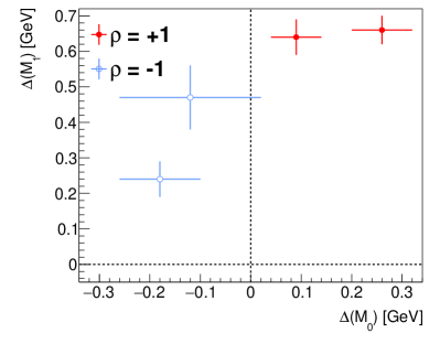
(a) $M_{\mathrm{0}}$ vs. $M_{\mathrm{1}}$

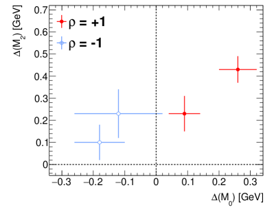
(b) $M_{\mathrm{0}}$ vs. $M_{\mathrm{2}}$

Figure 3: The sources of systematic uncertainties with estimator correlations of $\rho_{ijk}=+1$ (full red points) or $\rho_{ijk}=-1$ (open blue points). The points indicate the size of the uncertainties and the bars their statistical precision. In each of the figures, from right to left the points correspond to the sources $\mathrm{Syst}_{1}$ to $\mathrm{Syst}_{4}$ from Table 1.

The sources of systematic uncertainties for which the estimator correlations are $\rho_{ijk}=\pm 1$ are shown in Fig. 3. The case $\rho_{ijk}=+1$ corresponds to the situation where simultaneously applying a systematic effect to both estimates (e.g. increasing a component $l$ of the jet energy scale uncertainty by $+1\sigma_{\mathrm{JES,l}}$ as e.g. performed in Ref. [5]) leads to both measured values moving into the same direction, either both get larger or both get smaller than the original result. The case $\rho_{ijk}=-1$ means the two measurements move in opposite directions. See Ref. [5] for further details. The points for which the bars cross one of the coordinate axis indicate sources for which, within uncertainties, the correlation may be $\rho_{ijk}=+1$ or $\rho_{ijk}=-1$. For example, this is the case for $\mathrm{Syst}_{3}$ of $M_{\mathrm{0}}$ from Table 1, i.e. for the upper point in the left quadrant in both subfigures of Fig. 3. This will be exploited in the stability evaluation discussed below.

Without combining, the precision of the knowledge about the observable is defined by the most precise result, here $M_{\mathrm{2}}$. The impact that an additional estimate has can be digested by performing pairwise combinations with the most precise result. An example of such a pairwise combination of $M_{\mathrm{0}}$ and $M_{\mathrm{2}}$ is shown in Fig. 4. Apart from the range $\rho>0.8$, the combined value is almost independent of $\rho$. In contrast, the uncertainty in the combined value has a very strong dependence on $\rho$.

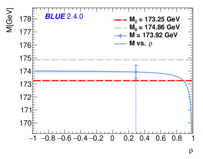
(a) Combined value

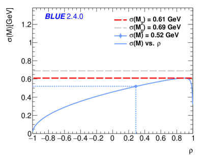
(b) Uncertainty in the combined value

Figure 4: Results of the combination of the estimates $M_{\mathrm{0}}$ and $M_{\mathrm{2}}$ as functions of $\rho$, where the blue point corresponds to the actual correlation $\rho(M_{\mathrm{0}},M_{\mathrm{2}})$. The combined value is shown in (a), the uncertainty in the combined value in (b).

The combination of all estimates is shown in Fig. 5(a). The input measurements are listed in the first three lines, the combined result is listed in red in the last line. Fig. 5(b) reveals that not all results significantly contribute to the combined value. In this figure, the lines show the results of successive combinations, always adding the estimate listed, to the previous list of estimates. Also here, the suggested combined result is shown in red. At the quoted precision, the estimate $M_{\mathrm{1}}$ does not improve the already accumulated result obtained from combining $M_{\mathrm{2}}$ and $M_{\mathrm{0}}$. This means $M_{\mathrm{1}}$ merely serves as a cross-check measurement for the combination.

Fig. 6 shows the stability of the combination of all three results, taking into account the statistical precisions at which the systematic uncertainties are known, see Table 1. For this figure, all systematic uncertainties are altered within their statistical precisions. For sources with $\rho_{ijk}=\pm 1$ also the correlations are re-evaluated, i.e. they may change sign, see Fig. 3. The varied input measurements are combined. The resulting combined values and uncertainties in the combined values are shown in the histograms. For the statistical precision at which the uncertainties are known, the combined result is uncertain by $0.15$ GeV and the related uncertainty by $0.04$ GeV. These uncertainties exist on top of what is quoted in Table 1. Frequently those are not provided, or even not evaluated. This is only justified if they are much smaller than the quoted uncertainties. For the statistical uncertainty in the combined result of $0.20$ GeV, see Table 1, the situation is at the border of being acceptable.

4 Impact

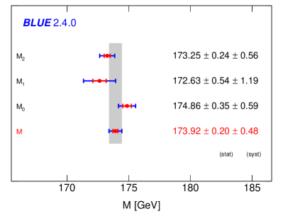
(a) Full combination

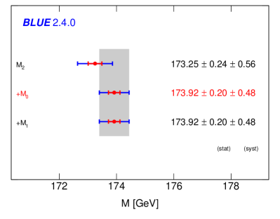
(b) Successive combination

Figure 5: The three estimates and the combined value of all estimates are shown in (a). In contrast, (b) shows the combined results obtained in successive combinations adding one estimate at a time, i.e. the second line is the result of combining $M_{\mathrm{2}}$ and $M_{\mathrm{0}}$, the third line the result of the combination of all three measurements.

The software can be used for an in-depth analysis of the impact of various assumptions made in the combination. In case the relevant input is provided, it also allows assessing the stability of the combination.

Because of the large reduction in the uncertainty in the combined result obtained by lowering the estimator correlations, see Fig. 4, it is advisable to use this software already in the design stage of the various analyses performed for obtaining the same observable within a single experiment. Usually, the uncertainties in the various systematic effects (e.g. the uncertainty in jet energy scales for experiments at hadron collider) are determined by the actual level of understanding of the detector and have to be taken into account at face value. In contrast, the sensitivity of the estimators to those effects can be influenced by the estimator design. This way their correlation can be reduced, thereby improving the gain obtained in the combination. Generally speaking, the strategy should not be to take over an aspect of the analysis that has worked for one estimator to another estimator. Instead, alternative approaches should be pursuit, such as to potentially lower the estimator correlations, even at the expense of a larger uncertainty. This is because achieving an anti-correlated pair of estimates with the same sensitivity to a specific source of uncertainty, renders this a significantly smaller uncertainty in the combined result. This can be seen for the sources $\mathrm{Syst}_{3}$ and $\mathrm{Syst}_{4}$, for which $\rho_{ij3}=\rho_{ij4}=-1$. Those sources exhibit the largest fractional gain in uncertainty when comparing $M$ with $M_{\mathrm{0}}$, e.g. $\sigma_{x4}/\sigma_{24}=0.02/0.10=1/5$.

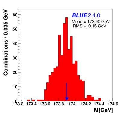
(a) Combined value

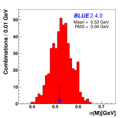
(b) Uncertainty in combined value

Figure 6: The stability of the combined value (a) and the uncertainty in the combined value (b), obtained in 500 combinations, while varying the input uncertainties and correlations according to their statistical precision.

An example of such an optimization is explained in Ref. [5]. This software can be of significant help in this process.

According to the knowledge of the author, by now the BLUE software was used in a number of combinations, mostly in the context of high energy physics, especially at the Large Hadron Collider (LHC). Examples from the ALICE, ATLAS, CMS and LHCb collaborations are detailed in Refs. [6, 7, 8, 9]. The first world combination of the top quark mass [10] has also been performed with this software. In addition to the LHC collaborations, the software has been used by the PHENIX [11] and STAR [12] collaborations, and in a combination of the strong coupling constant $\alpha_{s}$ from many results in Ref. [13]. Further examples of the software usage are described in the manual listed in the Code metadata table. To assist the users in developing their own combination code, the corresponding C++ routines to reproduce those published results are included in the software package. Although the above examples are all particle physics applications, the use of this software is not confined to a specific area of research. Any set of correlated measurements of one or more observables can be combined.

5 Conclusions

The software performs the combination of $m$ correlated estimates of $n$ physics observables ($m\geq n$) using the Best Linear Unbiased Estimate (BLUE) method. The large flexibility, together with the several implemented correlation models and combination methods makes it a useful tool to assess details on the combination in question. Exploring the combination of various estimators of the same observable within a single experiment allows a design of estimators with low correlation. This enhances the gain achieved in combinations of estimates obtained from those estimators.

Declaration of competing interest

The author declares that he has no known competing financial interests or personal relationships that could have appeared to influence the work reported in this paper.

Appendix A Example code

Listing 1: B_SoftExample.inp

⬇

1// Load Blue library

2gSystem->Load(”libBlue.so”);

3

4// Compile and execute code. This will produce

5// the below ’.cxx’ files and a ’.tex’ file

6.L B_SoftExample.cxx++

7 B_SoftExample()

8

9// Figure 3a

10.L B_SoftExample_x0_x1_CorPai.cxx++

11 B_SoftExample_x0_x1_CorPai()

12

13// Figure 3b

14.L B_SoftExample_x0_x2_CorPai.cxx++

15 B_SoftExample_x0_x2_CorPai()

16

17// Figure 4a,b

18.L B_SoftExample_x0_x2_DisPai.cxx++

19 B_SoftExample_x0_x2_DisPai()

20

21// Figure 5a

22.L B_SoftExample_DisRes_Obs_0.cxx++

23 B_SoftExample_DisRes_Obs_0()

24

25// Figure 5b

26.L B_SoftExample_AccImp_Obs_0.cxx++

27 B_SoftExample_AccImp_Obs_0()

28.q

Listing 2: B_SoftExample.cxx

⬇

1#include ”Blue.h”

2

3void B_SoftExample(){

4

5 //– Start preparing the inputs for later use in BLUE

6 // Numbers of estimates, uncertainties and observables

7 static const Int_t NumEst = 3;

8 static const Int_t NumUnc = 6;

9 static const Int_t NumObs = 1;

10

11 // Array of names of estimates (i,j = 0, 1, 2)

12 static const TString NamEst[NumEst] = {”M_{0}”, ”M_{1}”, ”M_{2}”};

13

14 // Array of names of uncertainties (k = 0, …, 5)

15 static const TString NamUnc[NumUnc] = {

16 ”Stat”, ”Syst_{1}”, ”Syst_{2}”, ”Syst_{3}”, ”Syst_{4}”, ”Syst_{5}”};

17

18 // Array of names of observables (n = 0)

19 static const TString NamObs[NumObs] = {”M”};

20

21 // Array of estimates and uncertainties, copy to matrix

22 static const Int_t LenXEst = NumEst * (NumUnc+1);

23 static const Double_t XEst[LenXEst] = {

24 // Stat Sys1 Sys2 Sys3 Sys4 Sys5

25 174.86, 0.35, 0.26, 0.09, 0.12, 0.18, 0.48,

26 172.63, 0.54, 0.66, 0.64, 0.47, 0.24, 0.53,

27 173.25, 0.24, 0.43, 0.23, 0.23, 0.10, 0.12};

28 TMatrixD* InpEst = new TMatrixD(NumEst, NumUnc+1, &XEst[0]);

29

30 // Array of statistical precision in systematic uncertainties, copy to matrix

31 static const Int_t LenSUnc = NumEst * NumUnc;

32 static const Double_t SUnc[LenSUnc] = {

33 //Stat Sys1 Sys2 Sys3 Sys4 Sys5

34 0.00, 0.06, 0.05, 0.14, 0.08, 0.09,

35 0.00, 0.04, 0.05, 0.09, 0.05, 0.08,

36 0.00, 0.06, 0.08, 0.11, 0.08, 0.05};

37 TMatrixD* InpSta = new TMatrixD(NumEst, NumUnc, &SUnc[0]);

38

39 // Array of rho_ijk == const correlations for k < 5

40 static const Double_t RhoVal[NumUnc-1] = {

41 0.0, 1.0, 1.0, -1.0, -1.0};

42

43 // Array for correlation matrix for k == 5 with rho_ij5 != const

44 static const Int_t LenInd = NumEst * (NumEst-1) / 2;

45 static const Double_t RhoInd[LenInd] = {0.5, 0.6, -0.3};

46

47 // Formats and file name for figures and Latex file

48 static const TString ForVal = ”%5.2f”;

49 static const TString ForUnc = ”%4.2f”;

50 static const TString ForWei = ForUnc;

51 static const TString ForRho = ”%+4.2f”;

52 static const TString ForPul = ForUnc;

53 static const TString ForChi = ForUnc;

54 static const TString ForUni = ”GeV”;

55 static const TString FilBas = ”B_SoftExample”;

56

57 // Axis ranges for Figs.3ab and Fig.6ab

58 static const Double_t XvaMax = 0.34, YvaMin = -0.05, YvaMax = 0.72;

59 static const Double_t ValMin = 173.2, ValMax = 174.6;

60 static const Double_t UncMin = 0.34, UncMax = 0.76;

61 //– End of preparation of inputs for BLUE

62

63 //– Start using BLUE — no inputs below this line —

64 //– Keywords: relate to the flowchart of the software

65 // Create: call constructor of BLUE object

66 Blue *myBlue = new Blue(NumEst, NumUnc);

67

68 // Fill: set display formats and define names

69 myBlue->SetFormat(ForVal, ForUnc, ForWei, ForRho, ForPul, ForChi, ForUni);

70 myBlue->FillNamEst(&NamEst[0]);

71 myBlue->FillNamUnc(&NamUnc[0]);

72 myBlue->FillNamObs(&NamObs[0]);

73

74 // Fill: insert estimates with their uncertainties

75 myBlue->FillEst(InpEst);

76

77 // Fill: insert statistical precision in systematic uncertainties

78 myBlue->FillSta(InpSta);

79

80 // Fill: insert the estimator correlations for all sources of uncertainty

81 for(Int_t k = 0; k<NumUnc; k++){

82 if(k != 5){myBlue->FillCor(k, RhoVal[k]);

83 }else{myBlue->FillCor(-k, &RhoInd[0]);}

84 }

85

86 // Change:

87 // … alterations would go here

88

89 // Fix:

90 myBlue->FixInp();

91

92 // Combine:

93 myBlue->Solve();

94

95 // Digest: show some estimate quantities, prepare code for Figs. 3 and 4

96 myBlue->PrintEst();

97 myBlue->CorrelPair(0, 1, FilBas, -XvaMax, XvaMax, YvaMin, YvaMax);

98 myBlue->CorrelPair(0, 2, FilBas, -XvaMax, XvaMax, YvaMin, YvaMax);

99 myBlue->DisplayPair(0, 2, FilBas);

100

101 // Digest: show some observable quantities, prepare code for Fig. 5a

102 myBlue->PrintChiPro();

103 myBlue->DisplayResult(0, FilBas);

104

105 // Digest: write Latex file

106 myBlue->LatexResult(FilBas);

107

108 // Free:, Fix:, Combine: solve according to importance

109 myBlue->ReleaseInp();

110 myBlue->FixInp();

111 myBlue->SolveAccImp(0.1);

112

113 // Digest: prepare code for Fig. 5b

114 myBlue->DisplayAccImp(0, FilBas);

115

116 // Free:, Fix:, Combine: solve varying the systematic uncertainties

117 myBlue->ReleaseInp();

118 myBlue->FixInp();

119 myBlue->SolveScaSta();

120

121 // Digest: produce Fig. 6

122 myBlue->PrintScaSta(FilBas, ValMin, ValMax, UncMin, UncMax);

123

124 // Delete: delete object as well as local matrices and return

125 delete myBlue; myBlue = NULL;

126 InpEst->Delete(); InpEst = NULL;

127 InpSta->Delete(); InpSta = NULL;

128 return;

129};

References

- [1] L. Lyons, D. Gibaut and P. Clifford, How to combine correlated estimates of a single physical quantity, Nucl. Instr. and Meth. A 270 (1988) 110. doi:10.1016/0168-9002(88)90018-6.
- [2] A. Valassi, Combining correlated measurements of several different quantities, Nucl. Instr. and Meth. A 500 (2003) 391. doi:10.1016/S0168-9002(03)00329-2.
- [3] R. Brun and F. Rademakers, ROOT - An Object Oriented Data Analysis Framework, Nucl. Instr. and Meth. A 389 (1997) 81, Proceedings of AIHENP’96 Workshop, Lausanne, Sep. 1996. doi:10.1016/S0168-9002(97)00048-X.
- [4] R. Nisius, On the combination of correlated estimates of a physics observable, Eur. Phys. J. C 74 (2014) 3004. arXiv:1402.4016, doi:10.1140/epjc/s10052-014-3004-2.
- [5] ATLAS Collaboration, Measurement of the top quark mass in the and channels using ATLAS data, Eur. Phys. J. C 75 (2015) 330. arXiv:1503.05427, doi:10.1140/epjc/s10052-015-3544-0.
- [6] ALICE Collaboration, Neutral pion and meson production in p-Pb collisions at , Eur. Phys. J. C 78 (2018) 624. arXiv:1801.07051, doi:10.1140/epjc/s10052-018-6013-8.
- [7] ATLAS Collaboration, Measurement of the top quark mass in the lepton+jets channel from ATLAS data and combination with previous results, Eur. Phys. J. C 79 (2019) 290. arXiv:1810.01772, doi:10.1140/epjc/s10052-019-6757-9.
- [8] CMS Collaboration, Measurements of the and cross sections and limits on anomalous quartic gauge couplings at , JHEP 10 (2017) 072. arXiv:1704.00366, doi:10.1007/JHEP10(2017)072.
- [9] LHCb Collaboration, Measurement of the branching fractions of the decays , and , JHEP 03 (2019) 176. arXiv:1810.03138, doi:10.1007/JHEP03(2019)176.
- [10] ATLAS, CDF, CMS and DO Collaborations, First combination of Tevatron and LHC measurements of the top-quark mass (2014). arXiv:1403.4427.
- [11] PHENIX Collaboration, Measurement of -meson production at forward rapidity in p + p collisions at and its energy dependence from to 7 TeV, Phys. Rev. D 98 (2018) 092006. arXiv:1710.01656, doi:10.1103/PhysRevD.98.092006.
- [12] STAR Collaboration, production in U + U collisions at measured with the STAR experiment, Phys. Rev. C 94 (2016) 064904. arXiv:1608.06487, doi:10.1103/PhysRevC.94.064904.
- [13] D. d’Enterria and A. Poldaru, Strong coupling extraction from a combined NNLO analysis of inclusive electroweak boson cross sections at hadron colliders, submitted to JHEP, arXiv:1912.11733.