Nonparametric multivariate regression estimation for circular responses

Abstract

Nonparametric estimators of a regression function with circular response and $\mathbb{R}^{d}$-valued predictor are considered in this work. Local polynomial type estimators are proposed and studied. Expressions for their asymptotic biases and variances are derived, and some guidelines to select asymptotically local optimal bandwidth matrices are also given. The finite sample behavior of the proposed estimators is assessed through simulations and their performance is also illustrated with a real data set.

Keywords: linear-circular regression, multivariate regression, local polynomial estimators

Introduction

New challenges on regression modeling appear when trying to describe relations between variables and at least some of them do not belong to an Euclidean space. For example, in many situations, one can be interested in estimating regression curves where some or all of the involved variables are circular ones. The special nature of circular data (points on the unit circle; angles in $\mathbb{T}=[0,2\pi)$) relies on their periodicity, which requires ad hoc statistical methods to analyze them. Circular statistics is an evolving discipline, and several statistical techniques for linear data now may claim their circular analogues. Comprehensive reviews on circular statistics (or more general, directional data) are provided in Fisher (1995), Jammalamadaka and Sengupta (2001) or Mardia and Jupp (2009). Some recent advances in directional statistics are collected in Ley and Verdebout (2017). Examples of circular data arise in many scientific fields such as biology, studying animal orientation (Batschelet, 1981), environmental applications (SenGupta and Ugwuowo, 2006), or oceanography (as in Wang et al., 2015, among others). In this setting, when the circular variable is supposed to vary with respect to other covariates and the goal is to model such a relation, regression estimators for circular responses must be designed and analyzed.

Parametric approaches were originally considered in Fisher and Lee (1992) and Presnell et al. (1998), assuming a parametric (conditional) distribution model for the circular response. In this scenario, covariates are supposed to influence the response via the parameters of the conditional distribution (e.g. through the location parameter, as the simplest case, or through location and concentration, if a von Mises distribution is chosen). In a practical setting, in Scapini et al. (2002), the orientation of two species of sand hoppers, considering parametric multiple regression methods for circular responses, following the proposal in Presnell et al. (1998), is analyzed. A parametric multivariate circular regression problem was also studied in Kim and SenGupta (2017). Beyond parametric restrictions, flexible approaches are also feasible in this context, just imposing some regularity conditions on the regression function, but avoiding the assumption of a specific parametric family for the regression function or for the conditional distribution. Local estimators of the regression function for circular response and a single real-valued covariate were introduced in Di Marzio et al. (2013). The authors proposed local estimators for the regression function which are defined as the inverse tangent function of the ratio between two sample statistics, obtained as weighted sums of the sines and the cosines of the response, respectively.

In the present work, a regression model with circular response and $\mathbb{R}^{d}$-valued predictor is considered. When the response variable is circular, the usual target regression function (derived from a cosine risk measure) is given by the inverse tangent function of the ratio between the conditional expectation of the sine and the conditional expectation of the cosine of the response variable. In this context, nonparametric regression estimators are proposed and studied. Our proposal considers two (separate) regression models for the sine and cosine components, which are indeed regression models with real-valued responses. Then, nonparametric estimators for the regression function at hand are obtained by computing the inverse tangent function of the ratio of multivariate local polynomial estimators for the two regression functions of the sine and cosine models. This way, estimators are obtained generalizing, both for higher dimensions and for higher polynomial degrees, the structure of the estimators proposed in Di Marzio et al. (2013) for a linear-circular regression function. The approach of considering two flexible regression models for the sine and cosine components has been also explored in Jammalamadaka and Sarma (1993), where the objective is the estimation of a circular-circular regression function. In this case, the conditional expectations of the sine and the cosine of the response are approximated by trigonometric polynomials of a suitable degree. A similar approach has been also considered in Di Marzio et al. (2014), where the problem of nonparametrically estimating a spherical-spherical regression is addressed as a multi-output regression problem. In this case, each Cartesian coordinate of the spherical regression function is separately estimated, within a scheme of a regression with a linear response and a spherical predictor. A multivariate angular regression model for both angular and linear predictors was studied by Rivest et al. (2016). Maximum likelihood estimators for the parameters were derived under two von Mises error structures.

This paper is organized as follows. In Section 2, the multivariate linear-circular regression model considered in this paper is presented, jointly with the models for the sine and cosine components, establishing certain relations between their first and second order moments. In Section 3, the nonparametric estimators of the regression function are proposed. Section 3.1 and Section 3.2 contain the Nadaraya–Watson (NW) and local linear (LL) versions of these estimators, respectively, and include expressions for their asymptotic biases and variances. A local polynomial type estimator with a general degree $p$, for the univariate case $(d=1)$, is also analyzed in Section 3.3. The finite sample performance of the estimators is assessed through a simulation study, provided in Section 4. Finally, Section 5 shows a real data application about sand hoppers orientation.

The regression model with circular response

Let $\{(\mathbf{X}_{i},\Theta_{i})\}_{i=1}^{n}$ be a random sample from $(\mathbf{X},\Theta)$, where $\Theta$ is a circular random variable taking values on $\mathbb{T}=[0,2\pi)$, and $\mathbf{X}$ is a random variable with density $f$ supported on $D\subseteq\mathbb{R}^{d}$. Assume that $\Theta$ and $\mathbf{X}$ are related through the following regression model:

$$\Theta_{i}=[m(\mathbf{X}_{i})+{\varepsilon}_{i}](\mbox{{mod}}\,2\pi),\quad i=1,\dots,n,$$ (1)

where $m$ is a circular regression function, and the ${\varepsilon}_{i}$ are independent and identically distributed (i.i.d.) random angles (independent of the $X_{i}$) with zero mean direction and finite concentration. This implies that ${\rm E}[\sin(\varepsilon)\mid\mathbf{X}=\mathbf{x}]=0$ and $\ell(\mathbf{x})={\rm E}[\cos(\varepsilon)\mid\mathbf{X}=\mathbf{x}]<\infty$. Additionally, assume that $\sigma^{2}_{1}(\mathbf{x})={\rm Var}[\sin(\varepsilon)\mid\mathbf{X}=\mathbf{x}]<\infty$, $\sigma^{2}_{2}(\mathbf{x})={\rm Var}[\cos(\varepsilon)\mid\mathbf{X}=\mathbf{x}]<\infty$ and $\sigma_{12}(\mathbf{x})={\rm E}[\sin(\varepsilon)\cos(\varepsilon)\mid\mathbf{X}=\mathbf{x}]<\infty$. In equation (1), mod stands for the modulo operation.

The circular regression function $m$ in model (1) is the conditional mean direction of $\Theta$ given $\mathbf{X}$ which, at a point $\mathbf{x}$, can be defined as the minimizer of the risk ${\rm E}\{1-\cos[\Theta-m(\mathbf{X})]\mid\mathbf{X}=\mathbf{x}\}$, which is comparable to the $L_{2}$ risk in the circular setting. Specifically, the minimizer of this cosine risk is given by $m(\mathbf{x})=\mbox{atan2}[m_{1}(\mathbf{x}),m_{2}(\mathbf{x})]$, where $m_{1}(\mathbf{x})={\rm E}[\sin(\Theta)\mid\mathbf{X}=\mathbf{x}]$ and $m_{2}(\mathbf{x})={\rm E}[\cos(\Theta)\mid\mathbf{X}=\mathbf{x}]$, and the function $\mbox{atan2}(y,x)$ returns the angle between the $x$-axis and the vector from the origin to $(x,y)$. Then, replacing $m_{1}$ and $m_{2}$ by appropriate estimators, an estimator for $m$ can be directly obtained. In particular, a whole class of kernel-type estimators for $m$ at $\mathbf{x}\in D$ can be defined by considering local polynomial estimators for $m_{1}(\mathbf{x})$ and $m_{2}(\mathbf{x})$. Specifically, estimators of the form:

$$\hat{m}_{\mathbf{H}}(\mathbf{x};p)=\mbox{atan2}[\hat{m}_{1,\mathbf{H}}(\mathbf{x};p),\hat{m}_{2,\mathbf{H}}(\mathbf{x};p)]$$ (2)

are considered, where for any integer $p\geq 0$, $\hat{m}_{1,\mathbf{H}}(\mathbf{x};p)$ and $\hat{m}_{2,\mathbf{H}}(\mathbf{x};p)$ denote the $p$th order local polynomial estimators (with bandwidth matrix $\mathbf{H}$) of $m_{1}(\mathbf{x})$ and $m_{2}(\mathbf{x})$, respectively. The special cases $p=0$ and $p=1$ yield a NW (or local constant) type estimator and a LL type estimator of $m(\mathbf{x})$, respectively.

Notice that the proposed approach amounts to consider two (separate) regression models for the sine and cosine of $\Theta$ on $\mathbf{X}$. In particular, the following regression models for the sine component:

$$\sin(\Theta_{i})=m_{1}(\mathbf{X}_{i})+\xi_{i}\quad i=1,\dots,n,$$ (3)

and the cosine component:

$$\cos(\Theta_{i})=m_{2}(\mathbf{X}_{i})+\zeta_{i}\quad i=1,\dots,n,$$ (4)

are considered, where the $\xi_{i}$ and the $\zeta_{i}$ are i.i.d. error terms, satisfying ${\rm E}[\xi\mid\mathbf{X}=\mathbf{x}]={\rm E}[\zeta\mid\mathbf{X}=\mathbf{x}]=0$, $s_{1}^{2}(\mathbf{x})={\rm Var}[\xi\mid\mathbf{X}=\mathbf{x}]<\infty$, $s_{2}^{2}(\mathbf{x})={\rm Var}[\zeta\mid\mathbf{X}=\mathbf{x}]<\infty$ and $c(\mathbf{x})={\rm E}[\xi\zeta\mid\mathbf{X}=\mathbf{x}]<\infty$ at every $\mathbf{x}\in D$.

Using the sine and cosine addition formulas, it is easy to derive some equations relating certain functions referred to model (1), and to models (3) and (4). Specifically, defining $f_{1}(\mathbf{x})=\sin[m(\mathbf{x})]$ and $f_{2}(\mathbf{x})=\cos[m(\mathbf{x})]$, it holds that:

$$m_{1}(\mathbf{x})=f_{1}(\mathbf{x})\ell(\mathbf{x})\quad\mbox{and}\quad m_{2}(\mathbf{x})=f_{2}(\mathbf{x})\ell(\mathbf{x}).$$

Note that $f_{1}(\mathbf{x})$ and $f_{2}(\mathbf{x})$ correspond to the normalized versions of $m_{1}(\mathbf{x})$ and $m_{2}(\mathbf{x})$, respectively. Indeed, taking into account that $f_{2}^{2}(\mathbf{x})+f_{1}^{2}(\mathbf{x})=1$, it can be easily deduced that $\ell(\mathbf{x})=[m^{2}_{1}(\mathbf{x})+m_{2}^{2}(\mathbf{x})]^{1/2}$. Hence, $\ell(\mathbf{x})$ amounts to the mean resultant length of $\Theta$ given $\mathbf{X}=\mathbf{x}$, which, taking into account that ${\rm E}[\sin(\varepsilon)\mid\mathbf{X}=\mathbf{x}]=0$ is assumed, also corresponds to the mean resultant length of $\varepsilon$ given $\mathbf{X}=\mathbf{x}$. Additionally, the following explicit expressions for the conditional variances of the error terms involved in models (3) and (4) can be obtained:

$$s_{1}^{2}(\mathbf{x}) = f_{1}^{2}(\mathbf{x})\sigma^{2}_{2}(\mathbf{x})+2f_{1}(\mathbf{x})f_{2}(\mathbf{x})\sigma_{12}(\mathbf{x})+f_{2}^{2}(\mathbf{x})\sigma^{2}_{1}(\mathbf{x}),$$

$$s_{2}^{2}(\mathbf{x}) = f_{2}^{2}(\mathbf{x})\sigma^{2}_{2}(\mathbf{x})-2f_{2}(\mathbf{x})f_{1}(\mathbf{x})\sigma_{12}(\mathbf{x})+f_{1}^{2}(\mathbf{x})\sigma^{2}_{1}(\mathbf{x}),$$

as well as for the covariance between the error terms in (3) and (4):

$$c(\mathbf{x})=f_{1}(\mathbf{x})f_{2}(\mathbf{x})\sigma^{2}_{2}(\mathbf{x})-f_{1}^{2}(\mathbf{x})\sigma_{12}(\mathbf{x})+f_{2}^{2}(\mathbf{x})\sigma_{12}(\mathbf{x})-f_{1}(\mathbf{x})f_{2}(\mathbf{x})\sigma^{2}_{1}(\mathbf{x}).$$

In what follows, $\bm{\nabla}g(\mathbf{x})$ and $\bm{\mathcal{H}}_{g}(\mathbf{x})$ will denote the vector of first-order partial derivatives and the Hessian matrix of a sufficiently smooth function $g$ at $\mathbf{x}$, respectively. Moreover, for a vector $\mathbf{u}=(u_{1},\dots,u_{d})^{T}$ and an integrable function $g$, the multiple integral $\int\int\dots\int g(\mathbf{u})du_{1}du_{2}\dots du_{d}$ will be simply denoted as $\int g(\mathbf{u})d\mathbf{u}$. Finally, for any matrix $\mathbf{A}$, $\lvert\mathbf{A}\rvert$, $\mbox{tr}(\mathbf{A})$, $\lambda_{{\max}}(\mathbf{A})$ and $\lambda_{{\min}}(\mathbf{A})$ denote its determinant, trace, maximum eigenvalue and minimum eigenvalue, respectively.

Properties of kernel-type estimators

Asymptotic (conditional) bias and variance of the estimator given in (2) are derived in this section. We will focus on the cases in which $p=0$ and $p=1$. For this, the asymptotic properties of the corresponding NW and LL estimators of $m_{j}(\mathbf{x})$, $j=1,2$ are firstly recalled. These results are then used to obtain the asymptotic properties of the estimator presented in (2) with polynomial degrees $p=0$ and $p=1$. Finally, asymptotic properties of local polynomial estimators with arbitrary order $p$ and $D\subseteq\mathbb{R}$ are also studied.

Nadaraya–Watson type estimator

Considering models (3) and (4), local constant estimators for the regression functions $m_{j}$, $j=1,2$, at a given point $\mathbf{x}\in D\subseteq\mathbb{R}^{d}$, are respectively defined as:

$$\hat{m}_{j,\mathbf{H}}(\mathbf{x};0)=\left\{\begin{array}[]{lc}\dfrac{\sum_{i=1}^{n}K_{\mathbf{H}}(\mathbf{X}_{i}-\mathbf{x})\sin(\Theta_{i})}{\sum_{i=1}^{n}K_{\mathbf{H}}(\mathbf{X}_{i}-\mathbf{x})}&\text{if $j=1$},\\ \\ \dfrac{\sum_{i=1}^{n}K_{\mathbf{H}}(\mathbf{X}_{i}-\mathbf{x})\cos(\Theta_{i})}{\sum_{i=1}^{n}K_{\mathbf{H}}(\mathbf{X}_{i}-\mathbf{x})}&\text{if $j=2$},\end{array}\right.$$ (5)

where, for $\mathbf{u}\in\mathbb{R}^{d}$, $K_{\mathbf{H}}(\mathbf{u})=\lvert\mathbf{H}\rvert^{-1}K(\mathbf{H}^{-1}\mathbf{u})$ is the rescaled version of a $d$-variate kernel function $K$, and $\mathbf{H}$ is a $d\times d$ bandwidth matrix. The resulting estimator $\hat{m}_{\mathbf{H}}(\mathbf{x};0)$ of $m(\mathbf{x})$, obtained by plugging (5) in (2), corresponds to the multivariate version of the local constant estimator proposed in Di Marzio et al. (2013).

Next, the asymptotic conditional bias and variance expressions for $\hat{m}_{\mathbf{H}}(\mathbf{x};0)$ are derived. First, using standard theory on the multivariate NW estimator Härdle and Müller (2000), the asymptotic conditional bias and variance of $\hat{m}_{j,\mathbf{H}}(\mathbf{x};0)$, $j=1,2$, are obtained. This preliminary result is given in Proposition 1. The following assumptions on the design density, the kernel function and the bandwidth matrix are required.

1. The design density $f$ is continuously differentiable at $\mathbf{x}\in D$, and satisfies $f(\mathbf{x})>0$. Moreover, $s_{j}^{2}$ and all second-order derivatives of the regression functions $m_{j}$, for $j=1,2$, are continuous at $\mathbf{x}\in D$, and $s_{j}^{2}(\mathbf{x})>0$.

2. The kernel $K$ is a spherically symmetric density function, twice continuously differentiable and with compact support (for simplicity with a nonzero value only if $\lVert\mathbf{u}\rVert\leq 1$). Moreover, $\int\mathbf{u}\mathbf{u}^{T}K(\mathbf{u})d\mathbf{u}=\mu_{2}(K)\mathbf{I}_{d}$, where $\mu_{2}(K)\neq 0$ and $\mathbf{I}_{d}$ denotes the $d\times d$ identity matrix. It is also assumed that $R(K)=\int K^{2}(\mathbf{u})d\mathbf{u}<\infty$.

3. The bandwidth matrix $\mathbf{H}$ is symmetric and positive definite, with $\mathbf{H}\to 0$ and $n\lvert\mathbf{H}\rvert\to\infty$, as $n\to\infty$.

In assumption (A3), $\textbf{H}\to 0$ means that every entry of H goes to $0$. Notice that, since H is symmetric and positive definite, $\textbf{H}\to 0$ is equivalent to $\lambda_{{\max}}(\textbf{H})\to 0$. $\lvert\textbf{H}\rvert$ is a quantity of order $\mathcal{O}\left[\lambda_{{\max}}^{d}(\textbf{H})\right]$ since $\lvert\textbf{H}\rvert$ is equal to the product of all eigenvalues of H.

Proposition 1.

Given the random sample $\{(\mathbf{X}_{i},\Theta_{i})\}_{i=1}^{n}$ from a density supported on $D\times\mathbb{T}$, assume models $(\ref{model1})$ and $(\ref{model2})$. Under assumptions $({\rm A}1)$–$({\rm A}3)$, the asymptotic conditional bias of estimators $\hat{m}_{j,\mathbf{H}}(\mathbf{x};0)$, for $j=1,2$, at a point $\mathbf{x}$ in the interior of the support of $f$, is:

$${\rm E}[\hat{m}_{j,\mathbf{H}}(\mathbf{x};0)-m_{j}(\mathbf{x})\mid\mathbf{X}_{1},\ldots,\mathbf{X}_{n}] = \frac{1}{2}\mu_{2}(K)\mbox{tr}(\mathbf{H}^{2}\bm{\mathcal{H}}_{m_{j}}(\mathbf{x}))$$ (6)

$$+\frac{\mu_{2}(K)}{f(\mathbf{x})}\bm{\nabla}^{T}{m_{j}}(\mathbf{x})\mathbf{H}^{2}\bm{\nabla}f(\mathbf{x})$$

$$+\mathpzc{o}_{\mathbb{P}}[\mbox{tr}(\mathbf{H}^{2})],$$

and the conditional variance is:

$${\rm Var}[\hat{m}_{j,\mathbf{H}}(\mathbf{x};0)\mid\mathbf{X}_{1},\ldots,\mathbf{X}_{n}]=\frac{R(K)s_{j}^{2}(\mathbf{x})}{n\lvert\mathbf{H}\rvert f(\mathbf{x})}+\mathpzc{o}_{\mathbb{P}}\left(\frac{1}{n\lvert\mathbf{H}\rvert}\right).$$ (7)

Now, using expressions (6) and (7), the following theorem provides the asymptotic conditional bias and the asymptotic conditional variance of the estimator $\hat{m}_{\mathbf{H}}(\mathbf{x};0)$. Its proof is included in the final Appendix.

Theorem 1.

Given the random sample $\{(\mathbf{X}_{i},\Theta_{i})\}_{i=1}^{n}$ from a density supported on $D\times\mathbb{T}$, assume model $(\ref{model})$. Then, under assumptions $({\rm A}1)$–$({\rm A}3)$, the asymptotic conditional bias of estimator $\hat{m}_{\mathbf{H}}(\mathbf{x};0)$, at a fixed interior point $\mathbf{x}$ in the support of $f$, is given by:

$${\rm E}[\hat{m}_{\mathbf{H}}(\mathbf{x};0)-m(\mathbf{x})\mid\mathbf{X}_{1},\dots,\mathbf{X}_{n}] = \dfrac{1}{2}\mu_{2}(K){\rm tr}[\mathbf{H}^{2}{\bm{\mathcal{H}}}_{m}(\mathbf{x})]$$

$$+\dfrac{\mu_{2}(K)}{\ell(\mathbf{x})f(\mathbf{x})}{\bm{\nabla}}^{T}m(\mathbf{x})\mathbf{H}^{2}{\bm{\nabla}}(\ell f)(\mathbf{x})$$

$$+{o}_{\mathbb{P}}[{\rm tr}(\mathbf{H}^{2})],$$

and the asymptotic conditional variance is:

$${\rm Var}[\hat{m}_{\mathbf{H}}(\mathbf{x};0)\mid\mathbf{X}_{1},\dots,\mathbf{X}_{n}]=\dfrac{R(K)\sigma^{2}_{1}(\mathbf{x})}{n\lvert\mathbf{H}\rvert\ell^{2}(\mathbf{x})f(\mathbf{x})}+\mathpzc{o}_{\mathbb{P}}\left(\dfrac{1}{n\lvert\mathbf{H}\rvert}\right).$$

Remark 3.1.

Note that both the asymptotic conditional bias and the asymptotic conditional variance share the form of the corresponding quantities for the NW estimator of a regression function with real-valued response. In the asymptotic bias expression, both the gradient and the Hessian matrix of $m$ refer to a circular regression function. In addition, the asymptotic conditional variance depends on the ratio $\sigma^{2}_{1}(\mathbf{x})/\ell^{2}(\mathbf{x})$, accounting for the variability of the errors in model $(\ref{model})$.

From Theorem 1, it is possible to define the asymptotic (conditional) mean squared error ($\rm AMSE$) of $\hat{m}_{\mathbf{H}}(\mathbf{x};0)$, as the sum of the square of the main term of bias and the main term of the variance,

$$\mbox{AMSE}[\hat{m}_{\mathbf{H}}(\mathbf{x};0)]$$ (8)

$$= \Bigg{\{}\dfrac{1}{2}{\mu_{2}(K)}{\rm tr}[\mathbf{H}^{2}{\bm{\mathcal{H}}}_{m}(\mathbf{x})]+\dfrac{\mu_{2}(K)}{\ell(\mathbf{x})f(\mathbf{x})}{\bm{\nabla}}^{T}m(\mathbf{x})\mathbf{H}^{2}{\bm{\nabla}}(\ell f)(\mathbf{x})\Bigg{\}}^{2}+\dfrac{R(K)\sigma^{2}_{1}(\mathbf{x})}{n\lvert\mathbf{H}\rvert\ell^{2}(\mathbf{x})f(\mathbf{x})}$$

$$= \dfrac{1}{4}\mu^{2}_{2}(K){\rm tr}^{2}\Bigg{(}\mathbf{H}^{2}\left\{\dfrac{1}{\ell(\mathbf{x})f(\mathbf{x})}[{\bm{\nabla}}(\ell f)(\mathbf{x}){\bm{\nabla}}^{T}m(\mathbf{x})+{\bm{\nabla}}m(\mathbf{x}){\bm{\nabla}}^{T}(\ell f)(\mathbf{x})]+{\bm{\mathcal{H}}}_{m}(\mathbf{x})\right\}\Bigg{)}$$

$$+\dfrac{R(K)\sigma^{2}_{1}(\mathbf{x})}{n\lvert\mathbf{H}\rvert\ell^{2}(\mathbf{x})f(\mathbf{x})}.$$

The minimizer of equation (8), with respect to $\mathbf{H}$, provides an asymptotically optimal local bandwidth matrix for $\hat{m}_{\mathbf{H}}(\mathbf{x};0)$, which is given by:

$$\mathbf{H}_{\text{opt}}(\mathbf{x}) = h^{*}(\mathbf{x})\left[\tilde{\mathcal{B}}(\mathbf{x})\right]^{-1/2}$$ (9)

$$= \left[\dfrac{R(K)\sigma^{2}_{1}(\mathbf{x})}{nd\mu^{2}_{2}(K)f(\mathbf{x})}\lvert\tilde{\mathcal{B}}(\mathbf{x})\rvert^{1/2}\right]^{1/{d+4}}\cdot\left[\tilde{\mathcal{B}}(\mathbf{x})\right]^{-1/2},$$

where

$$\tilde{\mathcal{B}}(\mathbf{x})=\left\{\begin{array}[]{lcc}\mathcal{B}(\mathbf{x})&\text{ if }&\mathcal{B}(\mathbf{x})\text{ is positive definite,}\\ -\mathcal{B}(\mathbf{x})&\text{if}&\mathcal{B}(\mathbf{x})\text{ is negative definite,}\\ \end{array}\right.$$

with

$$\mathcal{B}(\mathbf{x})=\dfrac{1}{\ell(\mathbf{x})f(\mathbf{x})}[{\bm{\nabla}}(\ell f)(\mathbf{x}){\bm{\nabla}}^{T}m(\mathbf{x})+{\bm{\nabla}}m(\mathbf{x}){\bm{\nabla}}^{T}(\ell f)(\mathbf{x})]+{\bm{\mathcal{H}}}_{m}(\mathbf{x}).$$

This optimization result can be proved using Proposition 2.6 included in Liu (2001). Note that in the expression of $\mathbf{H}_{\text{opt}}(\mathbf{x})$, the matrix $\tilde{\mathcal{B}}(\mathbf{x})$ determines the shape and the orientation in the $d$-dimensional space of the covariate region which is used to locally compute the estimator. Such data regions for computing the estimator are ellipsoids in $\mathbb{R}^{d}$, being the magnitude of the axes controlled by $\tilde{\mathcal{B}}(\mathbf{x})$ . In the particular case of $\bm{H}=h\mathbf{I}_{d}$, the estimator $\hat{m}_{\mathbf{H}}(\mathbf{x};0)$, with $\mathbf{x}$ being an interior point of the support, achieves an optimal convergence rate of $n^{-4/(d+4)}$, which is the same as the one for the multivariate NW estimator with real-valued response.

Despite deriving the previous explicit expression for the local optimal bandwidth (9), its use in practice is limited given that it depends on unknown functions, such as the design density $f$ and the variance of the sine of the errors $\sigma_{1}^{2}$. In addition, when the goal is to reconstruct the whole regression function and the focus is not only set on a specific point, it is more usual in practice to consider a global bandwidth for estimation rather than pursuing an estimator based on local bandwidths. An asymptotic global optimal bandwidth matrix $\mathbf{H}$ could be obtained by minimizing a global error measurement (such as the integrated version of the AMSE). Again, this will depend on unknowns and, moreover, this optimization problem is not trivial, not being possible to obtain a closed form solution. Alternatively, a cross-validation criterion suitably adapted for this context can be used to select the bandwidth matrix. This is indeed the bandwidth selection method employed in our numerical analysis and our real data application. More details will be provided in Section 4.

Local linear type estimator

Similarly to the case when $p=0$, the local linear case, corresponding to $p=1$, is considered. Specifically, for models (3) and (4), the LL estimators of the regression functions $m_{j}$, $j=1,2$, at $\mathbf{x}\in D$, are defined by:

$$\hat{m}_{j,\mathbf{H}}(\mathbf{x};1)=\left\{\begin{array}[]{lc}\mathbf{e}_{1}^{T}(\bm{\mathcal{X}}_{\mathbf{x}}^{T}\bm{\mathcal{W}}_{\mathbf{x}}\mathcal{X})^{-1}\bm{\mathcal{X}}_{\mathbf{x}}^{T}\bm{\mathcal{W}}_{\mathbf{x}}\mathbf{\bm{\mathcal{S}}}&\text{if $j=1$},\\ \\ \mathbf{e}_{1}^{T}(\bm{\mathcal{X}}_{\mathbf{x}}^{T}\bm{\mathcal{W}}_{\mathbf{x}}\bm{\mathcal{X}}_{\mathbf{x}})^{-1}\bm{\mathcal{X}}_{\mathbf{x}}^{T}\bm{\mathcal{W}}_{\mathbf{x}}\mathbf{\bm{\mathcal{C}}}&\text{if $j=2$},\end{array}\right.$$ (10)

where $\mathbf{e}_{1}$ is a $(d+1)\times 1$ vector having 1 in the first entry and 0 in all other entries, $\bm{\mathcal{X}}_{\mathbf{x}}$ is a $n\times(d+1)$ matrix having $(1,(\mathbf{X}_{i}-\mathbf{x})^{T})$ as its $i$th row, $\bm{\mathcal{W}}_{\mathbf{x}}=\mbox{diag}\{K_{\mathbf{H}}(\mathbf{X}_{1}-\mathbf{x}),\dots,K_{\mathbf{H}}(\mathbf{X}_{n}-\mathbf{x})\}$, $\mathbf{\bm{\mathcal{S}}}=(\sin(\Theta_{1}),\dots,\sin(\Theta_{n}))^{T}$ and $\mathbf{\bm{\mathcal{C}}}=(\cos(\Theta_{1}),\dots,\cos(\Theta_{n}))^{T}$.

Using known asymptotic results for the multivariate local linear estimator (Ruppert and Wand, 1994), the asymptotic conditional bias and variance of $\hat{m}_{j,\mathbf{H}}(\mathbf{x};1)$, $j=1,2$, can be obtained. These expressions are provided in the following result.

Proposition 2.

Given the random sample $\{(\mathbf{X}_{i},\Theta_{i})\}_{i=1}^{n}$ from a density supported on $D\times\mathbb{T}$, assume models $(\ref{model1})$ and $(\ref{model2})$. Under assumptions $({\rm A}1)$–$({\rm A}3)$, asymptotic conditional bias of estimators $\hat{m}_{j,\mathbf{H}}(\mathbf{x};1)$, $j=1,2$, with $\mathbf{x}$ being a point in the interior of the support of $f$, is:

$${\rm E}[\hat{m}_{j,\mathbf{H}}(\mathbf{x};1)-m_{j}(\mathbf{x})\mid\mathbf{X}_{1},\ldots,\mathbf{X}_{n}] = \frac{1}{2}\mu_{2}(K)\mbox{tr}(\mathbf{H}^{2}\bm{\mathcal{H}}_{m_{j}}(\mathbf{x}))$$ (11)

$$+\mathpzc{o}_{\mathbb{P}}[\mbox{tr}(\mathbf{H}^{2})],$$

and the asymptotic conditional variance is:

$${\rm Var}[\hat{m}_{j,\mathbf{H}}(\mathbf{x};1)\mid\mathbf{X}_{1},\ldots,\mathbf{X}_{n}]=\frac{R(K)s_{j}^{2}(\mathbf{x})}{n\lvert\mathbf{H}\rvert f(\mathbf{x})}+\mathpzc{o}_{\mathbb{P}}\left(\frac{1}{n\lvert\mathbf{H}\rvert}\right).$$ (12)

The resulting estimator $\hat{m}_{\mathbf{H}}(\mathbf{x};1)$ of $m(\mathbf{x})$ given in (2) corresponds to the multivariate version of the local linear estimator proposed in Di Marzio et al. (2013). The following theorem provides the asymptotic conditional bias and the asymptotic conditional variance of this estimator. Its proof is included in the final Appendix.

Theorem 2.

Given the random sample $\{(\mathbf{X}_{i},\Theta_{i})\}_{i=1}^{n}$ from a density supported on $D\times\mathbb{T}$, assume model $(\ref{model})$. Then, under assumptions $({\rm A}1)$–$({\rm A}3)$, the asymptotic conditional bias of estimator $\hat{m}_{\mathbf{H}}(\mathbf{x};1)$, with $\mathbf{x}$ being a fixed interior point in the support of $f$, is given by:

$${\rm E}[\hat{m}_{\mathbf{H}}(\mathbf{x};1)-m(\mathbf{x})\mid\mathbf{X}_{1},\dots,\mathbf{X}_{n}]=\dfrac{1}{2}\mu_{2}(K){\rm tr}[\mathbf{H}^{2}{\bm{\mathcal{H}}}_{m}(\mathbf{x})]+\dfrac{\mu_{2}(K)}{\ell(\mathbf{x})}{\bm{\nabla}}^{T}m(\mathbf{x})\mathbf{H}^{2}{\bm{\nabla}}\ell(\mathbf{x})+\mathpzc{o}_{\mathbb{P}}[\mbox{tr}(\mathbf{H}^{2})],$$

while its asymptotic conditional variance is:

$${\rm Var}[\hat{m}_{\mathbf{H}}(\mathbf{x};1)\mid\mathbf{X}_{1},\dots,\mathbf{X}_{n}]=\dfrac{R(K)\sigma^{2}_{1}(\mathbf{x})}{n\lvert\mathbf{H}\rvert\ell^{2}(\mathbf{x})f(\mathbf{x})}+\mathpzc{o}_{\mathbb{P}}\left(\dfrac{1}{n\lvert\mathbf{H}\rvert}\right).$$

Remark 3.2.

Estimators $\hat{m}_{\mathbf{H}}(\mathbf{x};0)$ and $\hat{m}_{\mathbf{H}}(\mathbf{x};1)$ have the same leading terms in their asymptotic conditional variances, while their asymptotic conditional biases, also being of the same order, have different leading terms. In particular, the main term of the asymptotic conditional bias of $\hat{m}_{\mathbf{H}}(\mathbf{x};1)$ does not depend on the design density, $f$. Moreover, as a consequence of its definition, the LL type estimator, differently from the NW type one, automatically adapts to boundary regions, in the sense that for compactly supported $f$, the asymptotic conditional bias has the same order both for the interior and for the boundary of the support of $f$ (Ruppert and Wand, 1994).

Remark 3.3.

For $d=1$, asymptotic results for estimators having the same form as the univariate version of estimator (2) with $p=0$ and $p=1$, are provided in Di Marzio et al. (2013). Despite they used slightly different formulations for their nonparametric estimators, their results, at interior points, can be directly compared with those obtained in Theorems 1 and 2. This correspondence is immediately clear for the asymptotic bias terms. For the asymptotic variance, the equivalence between the expressions can be obtained considering the relations between the variance of the error term in model (1) with the variance of the error terms in models (3) and (4):

$$f_{1}^{2}(\mathbf{x})[m_{2}^{2}(x)+s_{2}^{2}(x)]+f_{2}^{2}(\mathbf{x})[m_{1}^{2}(x)+s_{1}^{2}(x)]-2f_{1}(\mathbf{x})f_{2}(\mathbf{x})[m_{1}(\textbf{x})m_{2}(\textbf{x})+{c}(\mathbf{x})]=\sigma^{2}_{1}(x)$$ (13)

As a consequence of Theorem 2, and similarly to the NW case, an asymptotically optimal local bandwidth can be also obtained for $\hat{m}_{\mathbf{H}}(\mathbf{x};1)$, which coincides with (9), but taking $\mathcal{B}(\mathbf{x})=\ell^{-1}(\mathbf{x})[{\bm{\nabla}}\ell(\mathbf{x}){\bm{\nabla}}^{T}m(\mathbf{x})+{\bm{\nabla}}m(\mathbf{x}){\bm{\nabla}}^{T}\ell(\mathbf{x})]+{\bm{\mathcal{H}}}_{m}(\mathbf{x})$.

Higher order polynomials

Standard local polynomial theory (Fan and Gijbels, 1996) can be used to generalize the above results to local polynomial estimators of arbitrary order $p$. Using similar arguments to those used to prove Theorems 11 and 2, it can be derived that the The conditional bias of the $p$th order polynomial type estimator given in (2) will be of order $\mathcal{\mathcal{O}}_{\mathbb{P}}\{[{\rm tr}(\mathbf{H}^{2})]^{(p+1)/2}\}$. Moreover, if $p$ is even, $f$ has a continuous derivative in a neighborhood of $\mathbf{x}$, and $\mathbf{x}$ is an interior point of the support of the design density $f$, then the bias will be of order $\mathcal{\mathcal{O}}_{\mathbb{P}}\{[{\rm tr}(\mathbf{H}^{2})^{p/2+1}]\}$. Here, following the lines in Ruppert and Wand (1994), we will only focus on the case $d=1$ to analyze asymptotically the nonparametric regression estimator given in (2) for $p>1$. In particular, the $p$th degree local polynomial estimators for $m_{j}$, $j=1,2$, at $x\in\mathcal{D}\subseteq\mathbb{R}$, are:

$$\hat{m}_{j,h}(x;p)=\left\{\begin{array}[]{lc}\mathbf{e}^{T}_{1}(\bm{\mathcal{X}}_{{x},p}^{T}\bm{\mathcal{W}}_{x}\bm{\mathcal{X}}_{{x},p})^{-1}\bm{\mathcal{X}}_{{x},p}^{T}\bm{\mathcal{W}}_{x}\bm{\mathcal{S}}&\text{if $j=1$}\\ \\ \mathbf{e}^{T}_{1}(\bm{\mathcal{X}}_{{x},p}^{T}\bm{\mathcal{W}}_{x}\bm{\mathcal{X}}_{{x},p})^{-1}\bm{\mathcal{X}}_{{x},p}^{T}\bm{\mathcal{W}}_{x}\bm{\mathcal{C}}&\text{if $j=2$}\end{array}\right.$$ (14)

where $\mathbf{e}_{1}$ is a $(p+1)\times 1$ vector having 1 in the first entry and zero elsewhere, $\bm{\mathcal{X}}_{{x},p}$ is for $n\times p$ matrix with the $(i,k)$th entry equal to $(X_{i}-x)^{k-1}$, and $\bm{\mathcal{W}}_{x}$ is a diagonal matrix of order $n$ with $(i,i)$th entry equal to $K_{h}(X_{i}-x)$, where $K_{h}(u)=1/hK(u/h)$, being $K$ a univariate kernel function, and $h$ the bandwidth or smoothing parameter. In this univariate framework, the $p$th degree local polynomial type estimator of $m$ at $x$, denoted by $\hat{m}_{h}(x;p)$, has the same expression as the one given in (2), but using estimators $\hat{m}_{j,h}(x;p)$, $j=1,2$, defined in $(\ref{locpoly})$, as the arguments of the atan2 function.

Let $K_{(p)}$ be the equivalent kernel function defined in Lejeune and Sarda (1992), which is a kernel of order $p+2$ when $p$ is even and of order $p+1$ otherwise. Let $\mu_{j}(K_{(p)})$ and $R(K_{(p)})$ denote the moment of order $j$ and the roughness of $K_{(p)}$, respectively. Under suitable adaptations of assumptions $({\rm A}1)$–$({\rm A}3)$ to the univariate case and using asymptotic results for standard local polynomial estimators of an arbitrary order $p$, the asymptotic conditional bias and variance of $\hat{m}_{j,h}(x;p)$, $j=1,2$, can be obtained. It is clear that the conditional asymptotic bias of $\hat{m}_{h}(x;p)$ will depend on whether the polynomial degree is even or odd. Since computations are tedious for high-order polynomials, asymptotic properties of estimator $\hat{m}_{h}(x;p)$ at $x\in\mathcal{D}$ will be derived only when the polynomial degree $p$ is equal to two and three. Notice that in the case of the regression function, Fan and Gijbels (1996) recommend to use polynomial orders $p=1$ or $p=3$ for estimating this curve. Results could be extended for higher-order polynomial degrees.

Theorem 3.

Let $\{(X_{i},\Theta_{i})\}_{i=1}^{n}$ be a random sample from a density defined on $\mathcal{D}\times\mathbb{T}$, with $\mathcal{D}\subseteq\mathbb{R}$, and let $x$ be an interior point of the support of the design density $f$. Under assumptions (A1)–(A3) with $d=1$, and assuming that $m_{j}$, $j=1,2$, admits continuous derivatives up to order four in a neighborhood of $x$, then

$${\mathbb{E}}[\hat{m}_{h}(x;2)-m(x)\mid X_{1},\ldots,X_{n}] = \frac{h^{4}\mu_{4}(K_{(2)})f^{\prime}(x)}{3!f(x)}[m^{(3)}(x)+a(x)]$$

$$+\frac{h^{4}\mu_{4}(K_{(2)})}{4!}[m^{(4)}(x)+b(x)]+{o}_{\mathbb{P}}\left(h^{4}\right),$$

and

$${\mathbb{V}{\rm ar}}[\hat{m}_{h}(x;2)\mid X_{1},\ldots,X_{n}]=\frac{R\left(K_{(2)}\right)}{nh\ell^{2}(x)f(x)}\sigma_{1}^{2}(x)+{o}_{\mathbb{P}}\left(\frac{1}{nh}\right),$$

where

$$a(x)=\dfrac{2\ell^{\prime\prime}(x)m^{\prime}(x)+4\ell^{\prime}(x)m^{\prime\prime}(x)}{\ell(x)}+\dfrac{m_{2}^{\prime\prime}(x)m_{1}^{\prime}(x)-m_{1}^{\prime\prime}(x)m_{2}^{\prime}(x)+2\ell^{\prime 2}(x)m^{\prime}(x)}{\ell^{2}(x)}$$

and

$$b(x) = \dfrac{2\ell^{(3)}(x)m^{\prime}(x)+6\ell^{\prime}(x)m^{(3)}(x)+6\ell^{\prime\prime}(x)m^{\prime\prime}(x)}{\ell(x)}$$

$$+\dfrac{2m_{2}^{(3)}(x)m_{1}^{\prime}(x)-2m_{1}^{(3)}(x)m_{2}^{\prime}(x)+6\ell^{\prime 2}(x)m^{\prime\prime}(x)+6\ell^{\prime}(x)\ell^{\prime\prime}(x)m^{\prime}(x)}{\ell^{2}(x)}$$

Theorem 4.

Let $\{(X_{i},\Theta_{i})\}_{i=1}^{n}$ be a random sample from a density defined on $\mathcal{D}\times\mathbb{T}$, with $\mathcal{D}\subseteq\mathbb{R}$, and let $x$ be an interior point of the support of the design density $f$. Under assumptions (A1)–(A3) with $d=1$, and assuming that $m_{j}$, $j=1,2$, admits continuous derivatives up to order five in a neighborhood of $x$, then

$${\mathbb{E}}[\hat{m}_{h}(x;3)-m(x)\mid X_{1},\ldots,X_{n}] = \frac{h^{4}\mu_{4}(K_{(3)})}{4!}[m^{(4)}(x)+b(x)]+{o}_{\mathbb{P}}\left(h^{4}\right),$$

and

$${\mathbb{V}{\rm ar}}[\hat{m}_{h}(x;3)\mid X_{1},\ldots,X_{n}]=\frac{R\left(K_{(3)}\right)}{nh\ell^{2}(x)f(x)}\sigma_{1}^{2}(x)+{o}_{\mathbb{P}}\left(\frac{1}{nh}\right).$$

Simulation study

In order to illustrate the performance of the estimators proposed in Section 3, a simulation study considering different scenarios is carried out for $d=2$ (that is, considering a circular response and a bidimensional covariate). For each scenario, 500 samples of size $n$ ($n=64,100,225$ and $400$) are generated on a bidimensional regular grid in the unit square considering the following regression models:

1. $\Theta=[\mbox{atan2}(6{X}_{1}^{5}-2{X}_{1}^{3}-1,-2{X}_{2}^{5}-3{X}_{2}-1)+\varepsilon](\mbox{{mod}}\,2\pi)$,

2. $\Theta=[\mbox{acos}({X}_{1}^{5}-1)+\dfrac{3}{2}\mbox{asin}({X}_{2}^{3}-{X}_{2}+1)+\varepsilon](\mbox{{mod}}\,2\pi)$,

where $\mathbf{X}=(X_{1},X_{2})$ denotes the bidimensional covariate, and the circular errors, $\varepsilon$, are drawn from a von Mises distribution $vM(0,\kappa)$ with different values of $\kappa$ (5, 10 and 15).

Figure 1 shows two realizations of simulated data (model M1: top row; model M2: bottom row). In both cases, the sample size is $n=225$. Left plots show the regression functions evaluated in the regularly spaced sample $(X_{1},X_{2})$. Central panels present the random errors generated from a von Mises distribution with zero mean direction and concentration $\kappa=5$, for model M1, and $\kappa=15$, for model M2. Right panels show the values of the response variables, obtained adding regression functions and circular errors. It can be seen that the errors in the top row, corresponding to $\kappa=5$, present more variability than the ones generated with $\kappa=15$.

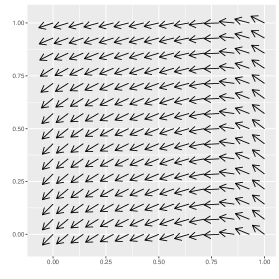
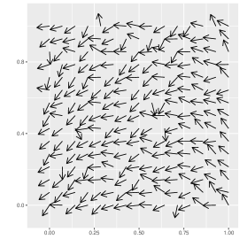
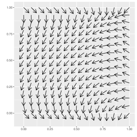
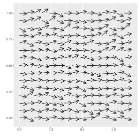
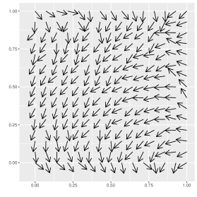
Figure 1: Illustration of model generation (model M1: top row; model M2: bottom row) on a $15\times 15$ grid. In left panels, regression functions evaluated at the grid points. In center panels, independent errors from a von Mises distribution with zero mean and concentration $\kappa=5$, for model M1, and $\kappa=15$, for model M2. In right panels, random response variables obtained by adding the two previous plots.

Numerical and graphical outputs summarize the finite sample performance of NW and LL type estimators in the different scenarios. In all cases, the smoothing parameter is chosen by cross-validation, selecting the bandwidth matrix $\mathbf{H}$ that minimizes the function:

$${\rm CV}(\mathbf{H})=\sum_{i=1}^{n}\left\{1-\cos\left[\Theta_{i}-\hat{m}_{\mathbf{H}}^{(i)}(\mathbf{X}_{i};p)\right]\right\},$$

where $\hat{m}_{\mathbf{H}}^{(i)}(\cdot;p)$ stands for the NW type estimator ($p=0$) or the LL type estimator ($p=1$), computed using all observations except $(\mathbf{X}_{i},\Theta_{i})$. Taking into account the type of regression functions considered in models M1 and M2 and to speed up the computing times, in this simulation study, the bandwidth matrix is restricted to be diagonal with possibly different elements. A multivariate Epanechnikov kernel is considered for simulations.

Table 1 shows the average, over the 500 replicates, of the circular average squared error (CASE), defined as:

$${\rm CASE}[\hat{m}_{\mathbf{H}}(\mathbf{x};p)]=\frac{1}{n}\sum_{i=1}^{n}\left\{1-\cos\left[m(\mathbf{X}_{i})-\hat{m}_{\mathbf{H}}(\mathbf{X}_{i};p)\right]\right\},$$ (15)

for models M1 and M2, and $p=0$ (NW) and $p=1$ (LL). It can be seen that this average error decreases with the sample size, and it is smaller for the LL type estimator in all the considered scenarios.

$\kappa$	$n$			M1					M2
			NW		LL			NW		LL
5	64		0.0225		0.0233			0.0366		0.0282
	100		0.0170		0.0164			0.0387		0.0208
	225		0.0057		0.0049			0.0184		0.0102
	400		0.0055		0.0049			0.0128		0.0073
10	64		0.0120		0.0124			0.0212		0.0143
	100		0.0107		0.0085			0.0023		0.0012
	225		0.0048		0.0038			0.0124		0.0060
	400		0.0034		0.0025			0.0079		0.0042
15	64		0.0088		0.0088			0.0164		0.0106
	100		0.0079		0.0060			0.0151		0.0082
	225		0.0037		0.0028			0.0107		0.0046
	400		0.0025		0.0017			0.0061		0.0032

Table 1: Average error (over $500$ replicates) of the CASE given in (15), for regression models M1 and M2, using NW and LL type estimators. Errors are generated from a von Mises distribution with different concentration parameters ($\kappa=5,10,15$). Bandwidth matrix is selected by cross-validation.

Numerical outputs are completed with some additional plots. As an illustration of the correct performance of NW and LL type estimators, Figure 2 shows the theoretical regression functions for models M1 and M2 (left panels) and the corresponding average, over 500 replicates, of the estimates, using the specific scenarios considered in Figure 1 (NW and LL estimates in the center and right panels, respectively). Notice that, for comparison purposes, the theoretical regression functions are plotted in a $100\times 100$ regular grid of the explanatory variables (the same grid where the estimations were computed). Plots in the top row present the results for the data generated from model M1 and those in the bottom row for model M2. Although both estimators have a similar and correct behavior, the LL estimator seems to show a slightly better performance, at least, for these samples. More reliable comparisons between NW and LL type estimators can be performed computing the circular bias (CB), the circular variance (CVAR), and the circular mean squared error (CMSE) for both estimators, in a grid of values of the explanatory variables. These quantities, at a point $\mathbf{x}$, are defined as:

$${\rm CB}[\hat{m}_{\mathbf{H}}(\mathbf{x};p)]={\rm E}\{\sin[\hat{m}_{\mathbf{H}}(\mathbf{x};p)-m(\mathbf{x})]\},$$ (16)

$${\rm CVAR}[\hat{m}_{\mathbf{H}}(\mathbf{x};p)]={\rm E}\{1-\cos[\hat{m}_{\mathbf{H}}(\mathbf{x};p)-\mu(\mathbf{x;p})]\},$$ (17)

$${\rm CMSE}[\hat{m}_{\mathbf{H}}(\mathbf{x};p)]={\rm E}\{1-\cos[m(\mathbf{x})-\hat{m}_{\mathbf{H}}(\mathbf{x};p)]\},$$ (18)

where $\mu(\mathbf{x;p})$ in CVAR denotes the circular mean of $\hat{m}_{\mathbf{H}}(\mathbf{x};p)$. Notice that, using Taylor expansions, equations (16), (17) and (18) are equivalent to the Euclidean versions of these expressions (Kim and SenGupta, 2017).

Figures 3 and 4 show, in the scenarios considered in Figure 1, the CB, CVAR and CMSE computed in a $100\times 100$ regular grid of the explanatory variables, when using NW (top row) and LL (bottom row) fits, for models M1 and M2, respectively. The expectations in (16), (17) and (18) are approximated by the averages over the 500 replicates generated. It can be seen that the NW type estimator ($p=0$) provides larger biases and smaller variances than the LL type estimator ($p=1$) in both settings. However, the CMSE is smaller for the LL fit in most of the grid points. Similar results for the CB, CVAR and CMSE for both estimators were obtained in other scenarios.

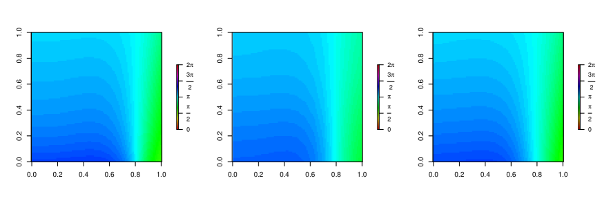
Figure 2: Theoretical regression function (left), jointly with the average, over 500 replicates, of NW (center) and LL (right) estimates, using the specific scenarios considered in Figure 1, for model M1 (top row) and model M2 (bottom row).

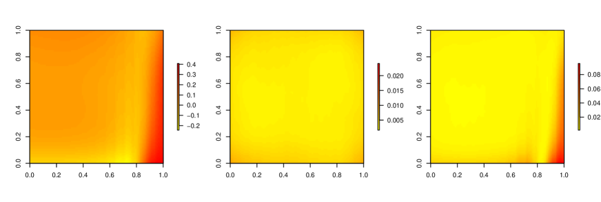
Figure 3: Circular bias (left), circular variance (center) and CMSE (right) surfaces for model M1 for a $100\times 100$ regular grid, using NW (top row) and LL (bottom row) fits. $n=225$ and von Mises errors with zero mean and $\kappa=5$.

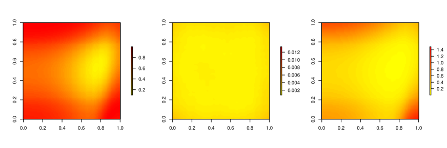
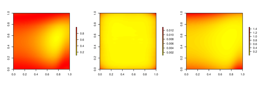
Figure 4: Circular bias (left), circular variance (center) and CMSE (right) surfaces for model M2 for a $100\times 100$ regular grid, using NW (top row) and LL (bottom row) fits. $n=225$ and von Mises errors with zero mean and $\kappa=15$.

Real data example

A real data example is presented in order to illustrate the application of the proposed estimators. Based on the simulation study, where the LL type estimator presented a slightly better performance than the NW one, just results corresponding to $\hat{m}_{\mathbf{H}}(\mathbf{x};1)$ are provided for real data. The orientation of two species of sand hoppers, considering parametric multiple regression methods for circular responses, following the proposal in Presnell et al. (1998), were analyzed in Scapini et al. (2002). This is a parametric approach that assumes a projected normal distribution for the scape directions and the corresponding parameters (circular mean and mean resultant vector) depend on the explanatory variables through a linear model. We refer to Scapini et al. (2002) and Marchetti and Scapini (2003) for details on the experiment, a thorough data analysis and sound biological conclusions. Dealing with the same data set, in Marchetti and Scapini (2003), the authors conclude that the orientation is different for the two sexes (males and females) and they explicitly mention that nonparametric smoothers are flexible tools that may suggest unexpected features of the data. So, the illustration with our proposal is a first attempt to analyze this data set with nonparametric tools in order to check how orientation (in degrees) behaves when temperature (in Celsius degrees) and (relative) humidity (in percentage) are included as covariates. For illustration purposes, only observations corresponding to (relative) humidity values larger than 45% are considered in this analysis. The corresponding data sets are plotted in Figure 5 (males in the left panel and females in the right panel), being the sample sizes $n=330$ and $n=404$, for male and female sand hoppers, respectively.

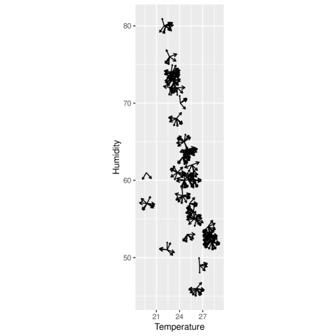
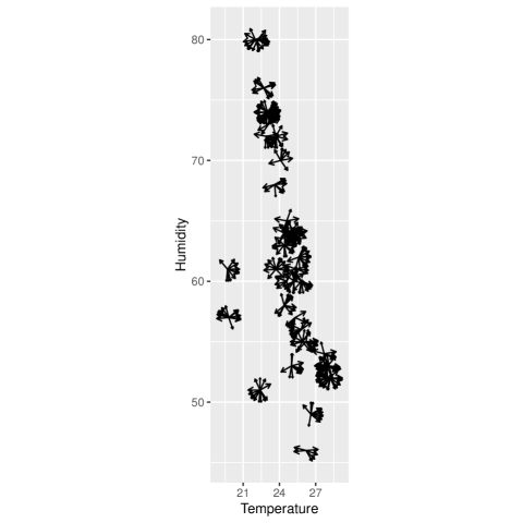
Figure 5: Observed orientation of male (left) and female (right) sand hoppers as a function of temperature and relative humidity.

Figure 6 shows the LL estimates for male (left) and female (right) mean orientations, considering temperature (horizontal axis) and relative humidity (vertical axis) as covariates. Note that measurements of temperature and humidity are the same for males and females, given that these values correspond to experimental conditions. In this example, unlike in the simulation experiments, the CV bandwidth matrix has been searched in the family of the symmetric and definite positive full bandwidth matrices, using an optimization algorithm based on the Nelder–Mead simplex method described in Lagarias et al. (1998). Using the initial bandwidth matrix $\mathbf{H}_{init}=1.5\cdot\mbox{diag}\left\{\hat{\sigma}_{X_{1}},\hat{\sigma}_{X_{2}}\right\}$, the algorithm converged to

$$\mathbf{H}_{\rm CV}^{m}=\left[\begin{array}[]{cc}2.7781&0.0001\\ 0.0001&15.2529\end{array}\right],$$

for males, and to

$$\mathbf{H}_{\rm CV}^{f}=\left[\begin{array}[]{cc}4.0930&-0.0009\\ -0.0009&13.1937\end{array}\right],$$

for females, where $\hat{\sigma}_{X_{1}}$ and $\hat{\sigma}_{X_{2}}$ denote the sample standard deviations of the covariates $X_{1}=$“temperature” and $X_{2}=$“humidity”, respectively. As in the previous section, a multivariate Epanechnikov kernel is considered. Note that the estimation grid of explanatory variables on which the estimates of the mean were computed was constructed by overlying the survey values of temperature and humidity with a $100\times 100$ grid and, then, dropping every grid point that did not satisfy one of the following two requirements: (a) it is within 15 “grid cell length” from an observation point, or (b) the calculation for the estimates of the sine and cosine components at that grid point uses a smoothing vector that is sufficiently stable. Both requirements are admittedly somewhat arbitrary, but they represent a compromise between coverage over the region of interest and ability to avoid singular design matrices. Even with these restrictions, some of the estimates for low temperature values (around 20 Celsius degrees) seem to be spurious, specially in the case of male individuals. This can be due to data sparseness or a boundary effect, two well-known situations where kernel-based smoothing methods may present certain drawbacks. Trying to avoid some of these problems and taking into account that there are repeated values of the covariates, possibly due to rounded measurements, additional estimates have been obtained after jittering the original data (the corresponding plots are not shown), obtaining estimates that follow similar patterns to those shown in Figure 6. The mean direction followed by male and female sand hoppers is different for some temperature and humidity conditions. Seawards orientation was roughly $7\pi/4$, so it can be seen that females are more seawards oriented than males, specially for mid to low values of temperature.

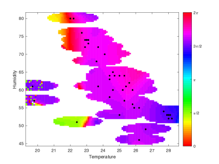
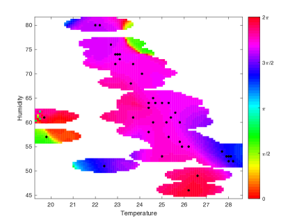
Figure 6: Estimates of the mean orientation of males (left) and females (right) sand hoppers, considering a LL estimator with cross-validation bandwidth. Horizontal axis: temperature, in Celsius degrees. Vertical axis: relative humidity, in percentage.

Discussion

Nonparametric regression estimation for circular responses and $\mathbb{R}^{d}$-valued covariates is studied in this paper. Our proposal considers kernel-based approaches, with special attention on NW and LL type estimators in general dimension, and for higher order polynomials in the one-dimensional case. Asymptotic conditional bias and variance are derived and the performance of the estimators is assessed in a simulation study.

For practical implementation, the selection of a $d$-dimensional bandwidth matrix is required. In the regression Euclidean context, the bandwidth selection problem has been widely addressed in the last decades (see, for example Köhler et al., 2014, where a review on bandwidth selection methods for kernel regression is provided). More related to the topic of the present paper, a rule-of-thumb and a bandwidth rule for selection scalar or diagonal bandwidth matrices for multivariate local linear regression with real-valued response and $\mathbb{R}^{d}$-valued covariate is derived in Yang and Tschernig (1999). Also in this context, in González-Manteiga et al., (2004), a bootstrap method to estimate the mean squared error and the smoothing parameter for the multidimensional regression local linear estimator is proposed. However, in the framework of nonparametric regression methods for circular variables, the research on bandwidth selection is very scarce or non-existent. Our practical results are derived with a cross-validation bandwidth given that, up to our knowledge, there are no other bandwidth selectors available in this context. The design of alternative procedures to select the bandwidth matrix for the estimators studied in this paper based, for example, on bootstrap methods are indeed of great interest. This problem is out of the scope of the present paper, but it is an interesting topic of research for a future study.

Once the problem of including a $\mathbb{R}^{d}$-valued covariate for explaining the behaviour of a circular response is solved, it seems natural to think about the consideration of covariates of different nature. Since the proposed estimator is constructed by considering the atan2 of the smooth estimators of the regression functions for the sine and cosine components of the response, an adaptation of our proposal for different types of covariates implies the use of suitable weights. For instance, if a spherical (circular, as a particular case) or a mixture of spherical and real-valued covariates are considered to influence a circular response, weights for estimating the sine and cosine components could be constructed following the ideas in García-Portugués et al. (2013) for cylindrical density estimation. If a categorical covariate is included in the model, a similar approach to the one in Racine and Li (2004) or in Li and Racine (2004) could be also followed. In all these cases, bandwidth matrices should be selected, and cross-validation techniques could be applied.

The results obtained in Theorem 3 and 4 can be extended to an arbitrary dimension $d$ of the space of the covariates by using the asymptotic properties for $\hat{m}_{j,\mathbf{H}}(\mathbf{x};p)$ provided in Gu et al. (2015) who considered the leading term of biases and variances of multivariate local polynomial estimators of general order $p$. Results on the asymptotic distribution of multivariate local polynomial estimators are also provided in Gu et al. (2015). The joint asymptotic normality of $\hat{m}_{1,\mathbf{H}}(\mathbf{x};p)$ and $\hat{m}_{2,\mathbf{H}}(\mathbf{x};p)$ can be used to derive, via the delta-method, the asymptotic distribution of statistics which can be expressed in terms of $\hat{m}_{1,\mathbf{H}}(\mathbf{x};p)$ and $\hat{m}_{2,\mathbf{H}}(\mathbf{x};p)$. For example, a suitable adaptation of Proposition 3.1 of Jammalamadaka and Sengupta (2001) can be used to derive the limiting distribution of the tangent of $\hat{m}_{\mathbf{H}}(\mathbf{x};p)$.

In our scenario, data generated from the regression model are assumed to be independent. However, in many practical situations, this assumption does not seem reasonable (e.g. data area collected over time or space). The simple construction scheme behind the proposed class of estimators makes possible to easily obtain asymptotic properties in more general frameworks. As an example, when data are not i.i.d. but are realizations of stationary processes satisfying some mixing conditions, the results provided in Masry (1996) can be used. It should be also noted that, when the data exhibit some kind of dependence, although the expression for the estimator will be the same, this structure will affect the estimator variance and should be taking into account to select properly the bandwidth parameter, as in Francisco-Fernandez and Opsomer (2005).

Appendix. Proof of the results

This section is devoted to present the proofs of Theorem 1, 2, 3 and 4. More specifically, the asymptotic properties of the proposed nonparametric regression estimator $\hat{m}_{\mathbf{H}}(\mathbf{x};p)$, for $p=0,1$, are established in Theorem 1 and 2, respectively. For $d=1$, the extensions for $p=2$ and $p=3$ are considered in Theorem 3 and 4, respectively.

Proof of Theorem 1.

First, to obtain the bias of $\hat{m}_{\mathbf{H}}(\mathbf{x};0)$, using the same linearization arguments as in the proof of Theorem $1$ of Di Marzio et al. (2013), $\mbox{atan2}(\hat{m}_{1,\mathbf{H}},\hat{m}_{2,\mathbf{H}})$ is expanded in Taylor series around $(m_{1},m_{2})$, where for simplicity, $\hat{m}_{j,\mathbf{H}}$ and $m_{j}$ denote $\hat{m}_{j,\mathbf{H}}(\mathbf{x})$ and $m_{j}(\mathbf{x})$, respectively, for $j=1,2$, to get

$$\mbox{atan2}(\hat{m}_{1,\mathbf{H}},\hat{m}_{2,\mathbf{H}}) = \mbox{atan2}(m_{1},m_{2})+\dfrac{m_{2}}{m_{1}^{2}+m_{2}^{2}}(\hat{m}_{1,\mathbf{H}}-m_{1})$$ (19)

$$-\dfrac{m_{1}}{m_{1}^{2}+m_{2}^{2}}(\hat{m}_{2,\mathbf{H}}-m_{2})+\dfrac{m_{1}m_{2}}{(m_{1}^{2}+m_{2}^{2})^{2}}(\hat{m}_{2,\mathbf{H}}-m_{2})^{2}$$

$$-\dfrac{m_{1}m_{2}}{(m_{1}^{2}+m_{2}^{2})^{2}}(\hat{m}_{1,\mathbf{H}}-m_{1})^{2}$$

$$-\dfrac{m_{1}^{2}-m_{2}^{2}}{(m_{1}^{2}+m_{2}^{2})^{2}}(\hat{m}_{1,\mathbf{H}}-m_{1})(\hat{m}_{2,\mathbf{H}}-m_{2})$$

$$+\mathcal{O}\left[(\hat{m}_{1,\mathbf{H}}-m_{1})^{3}\right]+\mathcal{O}\left[(\hat{m}_{2,\mathbf{H}}-m_{2})^{3}\right],$$

Taking expectations, noting that ${\rm E}\left[(\hat{m}_{j,\mathbf{H}}-m_{j})^{2}\mid\mathbf{X}_{1},\dots,\mathbf{X}_{n}\right]={\rm Var}(\hat{m}_{j,\mathbf{H}}\mid\mathbf{X}_{1},\dots,\mathbf{X}_{n})+[E(\hat{m}_{j,\mathbf{H}})-m_{j}\mid\mathbf{X}_{1},\dots,\mathbf{X}_{n}]^{2}$, and using the results in Proposition 1, it is obtained that

$${\rm E}[\hat{m}_{\mathbf{H}}(\mathbf{x};0)-m(\mathbf{x})\mid\mathbf{X}_{1},\dots,\mathbf{X}_{n}]$$

$$= \dfrac{1}{2}{\dfrac{m_{2}(\mathbf{x})}{m_{1}^{2}(\mathbf{x})+m_{2}^{2}(\mathbf{x})}\mu_{2}(K)\mbox{tr}\left[\mathbf{H}^{2}\bm{\mathcal{H}}_{m_{1}}(\mathbf{x})\right]}$$

$$+\dfrac{m_{2}(\mathbf{x})}{m_{1}^{2}(\mathbf{x})+m_{2}^{2}(\mathbf{x})}\dfrac{\mu_{2}(K)}{f(\mathbf{x})}\bm{\nabla}^{T}{m_{1}}(\mathbf{x})\mathbf{H}^{2}\bm{\nabla}{f}(\mathbf{x})$$

$$-\dfrac{1}{2}{\dfrac{m_{1}(\mathbf{x})}{m_{1}^{2}(\mathbf{x})+m_{2}^{2}(\mathbf{x})}\mu_{2}(K)\mbox{tr}\left[\mathbf{H}^{2}\bm{\mathcal{H}}_{m_{2}}(\mathbf{x})\right]}$$

$$-\dfrac{m_{1}(\mathbf{x})}{m_{1}^{2}(\mathbf{x})+m_{2}^{2}(\mathbf{x})}\dfrac{\mu_{2}(K)}{f(\mathbf{x})}\bm{\nabla}^{T}{m_{2}}(\mathbf{x})\mathbf{H}^{2}\bm{\nabla}{f}(\mathbf{x})$$

$$+{\mathpzc{o}_{\mathbb{P}}[\mbox{tr}(\mathbf{H}^{2})]}.$$

Therefore,

$${\rm E}[\hat{m}_{\mathbf{H}}(\mathbf{x};0)-m(\mathbf{x})\mid\mathbf{X}_{1},\dots,\mathbf{X}_{n}]$$

$$= \dfrac{1}{2}\dfrac{\mu_{2}(K)}{m_{1}^{2}(\mathbf{x})+m_{2}^{2}(\mathbf{x})}\mbox{tr}\bigg{\{}\mathbf{H}^{2}\bigg{[}m_{2}(\mathbf{x})\bm{\mathcal{H}}_{m_{1}}(\mathbf{x})-m_{1}(\mathbf{x})\bm{\mathcal{H}}_{m_{2}}(\mathbf{x})\bigg{]}\bigg{\}}$$

$$+\dfrac{\mu_{2}(K)}{[m_{1}^{2}(\mathbf{x})+m_{2}^{2}(\mathbf{x})]f(\mathbf{x})}\bigg{\{}\left[m_{2}(\mathbf{x})\bm{\nabla}^{T}{m_{1}}(\mathbf{x})-m_{1}(\mathbf{x})\bm{\nabla}^{T}{m_{2}}(\mathbf{x})\right]\mathbf{H}^{2}\bm{\nabla}{f}(\mathbf{x})\bigg{\}}$$

$$+{\mathpzc{o}_{\mathbb{P}}[\mbox{tr}(\mathbf{H}^{2})]}.$$

Now, taking into account that

$${\bm{\nabla}}m(\mathbf{x}) = \dfrac{1}{\ell^{2}(x)}\left[{\bm{\nabla}}m_{1}(\mathbf{x})m_{2}(\mathbf{x})-{\bm{\nabla}}m_{2}(\mathbf{x})m_{1}(\mathbf{x})\right],$$ (20)

$${\bm{\mathcal{H}}}_{m}(\mathbf{x}) = \dfrac{1}{\ell^{2}(x)}\left[{\bm{\mathcal{H}}}_{m_{1}}(\mathbf{x})m_{2}(\mathbf{x})+{\bm{\nabla}}m_{1}(\mathbf{x}){\bm{\nabla}}^{T}m_{2}(\mathbf{x})\right.$$ (21)

$$-\left.{\bm{\nabla}}m_{2}(\mathbf{x}){\bm{\nabla}}^{T}m_{1}(\mathbf{x})-{\bm{\mathcal{H}}}_{m_{2}}(\mathbf{x})m_{1}(\mathbf{x})\right]-\dfrac{2}{\ell(x)}{\bm{\nabla}}\ell(\mathbf{x}){\bm{\nabla}}^{T}m(x),$$

it follows that

$${\mathbb{E}}[\hat{m}_{\mathbf{H}}(\mathbf{x};0)-m(\mathbf{x})\mid\mathbf{X}_{1},\dots,\mathbf{X}_{n}] = \dfrac{1}{2}\mu_{2}(K){\rm tr}[\mathbf{H}^{2}{\bm{\mathcal{H}}}_{m}(\mathbf{x})]+\dfrac{\mu_{2}(K)}{\ell(\mathbf{x})f(\mathbf{x})}{\bm{\nabla}}^{T}m(\mathbf{x})\mathbf{H}^{2}{\bm{\nabla}}(\ell f)(\mathbf{x})$$

$$+\mathpzc{o}_{\mathbb{P}}[{\rm tr}(\mathbf{H}^{2})].$$

To derive the variance, the function $\mbox{atan2}^{2}(\hat{m}_{1,\mathbf{H}},\hat{m}_{2,\mathbf{H}})$ is expanded in Taylor series around $(m_{1},m_{2})$, to obtain

$$\mbox{atan2}^{2}(\hat{m}_{1,\mathbf{H}},\hat{m}_{2,\mathbf{H}}) = \mbox{atan2}^{2}({m}_{1},{m}_{2})+\dfrac{2\mbox{atan2}(m_{1},m_{2})m_{2}}{m_{1}^{2}+m_{2}^{2}}(\hat{m}_{1,\mathbf{H}}-{m}_{1})$$ (22)

$$-\dfrac{2\mbox{atan2}(m_{1},m_{2})m_{1}}{m_{1}^{2}+m_{2}^{2}}(\hat{m}_{2,\mathbf{H}}-{m}_{2})$$

$$+\dfrac{2\mbox{atan2}(m_{1},m_{2})m_{1}m_{2}}{(m_{1}^{2}+m_{2}^{2})^{2}}(\hat{m}_{2,\mathbf{H}}-{m}_{2})^{2}$$

$$-\dfrac{2\mbox{atan2}(m_{1},m_{2})m_{1}m_{2}}{(m_{1}^{2}+m_{2}^{2})^{2}}(\hat{m}_{1,\mathbf{H}}-{m}_{1})^{2}$$

$$-\dfrac{2\mbox{atan}(m_{1},m_{2})(m_{1}^{2}-m_{2}^{2})}{(m_{1}^{2}+m_{2}^{2})^{2}}(\hat{m}_{1,\mathbf{H}}-{m}_{1})(\hat{m}_{2,\mathbf{H}}-{m}_{2})$$

$$+\dfrac{m_{1}^{2}}{(m_{1}^{2}+m_{2}^{2})^{2}}(\hat{m}_{2,\mathbf{H}}-{m}_{2})^{2}+\dfrac{m_{2}^{2}}{(m_{1}^{2}+m_{2}^{2})^{2}}(\hat{m}_{1,\mathbf{H}}-{m}_{1})^{2}$$

$$-\dfrac{2m_{1}m_{2}}{(m_{1}^{2}+m_{2}^{2})^{2}}(\hat{m}_{1,\mathbf{H}}-{m}_{1})(\hat{m}_{2,\mathbf{H}}-{m}_{2})$$

$$+\mathcal{O}\left[(\hat{m}_{1,\mathbf{H}}-{m}_{1})^{3}\right]+\mathcal{O}\left[(\hat{m}_{2,\mathbf{H}}-{m}_{2})^{3}\right].$$

So, noting that ${\mathbb{V}{\rm ar}}(\hat{m}_{\mathbf{H}}\mid\mathbf{X}_{1},\dots,\mathbf{X}_{n})={\mathbb{E}}\left[(\hat{m}_{\mathbf{H}})^{2}\mid\mathbf{X}_{1},\dots,\mathbf{X}_{n}\right]-[\mathbb{E}(\hat{m}_{\mathbf{H}})\mid\mathbf{X}_{1},\dots,\mathbf{X}_{n}]^{2}$ and taking expectations in the Taylor expansions (19) and (22), it can be obtained that the conditional variance is:

$${\rm Var}[\hat{m}_{\mathbf{H}}(\mathbf{x};0)\mid\mathbf{X}_{1},\dots,\mathbf{X}_{n}]$$

$$= \dfrac{m_{1}^{2}(\mathbf{x})}{\left[m_{1}^{2}(\mathbf{x})+m_{2}^{2}(\mathbf{x})\right]^{2}}{\rm Var}[\hat{m}_{2,\mathbf{H}}(\mathbf{x};0)\mid\mathbf{X}_{1},\dots,\mathbf{X}_{n}]$$

$$+\dfrac{m_{2}^{2}(\mathbf{x})}{\left[m_{1}^{2}(\mathbf{x})+m_{2}^{2}(\mathbf{x})\right]^{2}}{\rm Var}[\hat{m}_{1,\mathbf{H}}(\mathbf{x};0)\mid\mathbf{X}_{1},\dots,\mathbf{X}_{n}]$$

$$-\dfrac{2m_{1}(\mathbf{x})m_{2}(\mathbf{x})}{\left[m_{1}^{2}(\mathbf{x})+m_{2}^{2}(\mathbf{x})\right]^{2}}\mbox{Cov}[\hat{m}_{1,\mathbf{H}}(\mathbf{x};0),\hat{m}_{2,\mathbf{H}}(\mathbf{x};0)\mid\mathbf{X}_{1},\dots,\mathbf{X}_{n}]$$

$$+\mathcal{O}\left[(\hat{m}_{1,\mathbf{H}}(\mathbf{x};0)-{m}_{1}(\mathbf{x}))^{3}\right]+\mathcal{O}\left[(\hat{m}_{2,\mathbf{H}}(\mathbf{x};0)-{m}_{2}(\mathbf{x}))^{3}\right].$$

Regarding the conditional covariance between $\hat{m}_{1,\mathbf{H}}(\mathbf{x};0)$ and $\hat{m}_{2,\mathbf{H}}(\mathbf{x};0)$, it follows that

$$\mbox{Cov}[\hat{m}_{1,\mathbf{H}}(\mathbf{x};0),\hat{m}_{2,\mathbf{H}}(\mathbf{x};0)\mid\mathbf{X}_{1},\dots,\mathbf{X}_{n}]$$ (23)

$$= \dfrac{\sum_{i=1}^{n}\sum_{j=1}^{n}K_{\mathbf{H}}(\mathbf{X}_{i}-\mathbf{x})K_{\mathbf{H}}(\mathbf{X}_{j}-\mathbf{x})}{\sum_{i=1}^{n}K_{\mathbf{H}}(\mathbf{X}_{i}-\mathbf{x})\sum_{j=1}^{n}K_{\mathbf{H}}(\mathbf{X}_{j}-\mathbf{x})}\mbox{Cov}[\sin(\Theta_{i}),\cos(\Theta_{j})\mid\mathbf{X}_{1},\dots,\mathbf{X}_{n}]$$

$$= \dfrac{\sum_{i=1}^{n}K^{2}_{\mathbf{H}}(\mathbf{X}_{i}-\mathbf{x})c(\mathbf{X}_{i})}{\left[\sum_{i=1}^{n}K_{\mathbf{H}}(\mathbf{X}_{i}-\mathbf{x})\right]^{2}}$$

$$= \dfrac{R(K)c(\mathbf{x})}{n\lvert\mathbf{H}\rvert f(\mathbf{x})}+\mathpzc{o}_{\mathbb{P}}\left(\dfrac{1}{n\lvert\mathbf{H}\rvert}\right).$$

Therefore, using (23) and Proposition 1, one gets that

$${\rm Var}[\hat{m}_{\mathbf{H}}(\mathbf{x};0)\mid\mathbf{X}_{1},\dots,\mathbf{X}_{n}] = \frac{1}{n\lvert\mathbf{H}\rvert}R(K)\dfrac{m_{1}^{2}(\mathbf{x})s_{2}^{2}(\mathbf{x})}{\left[m_{1}^{2}(\mathbf{x})+m_{2}^{2}(\mathbf{x})\right]^{2}f(\mathbf{x})}$$

$$+\frac{1}{n\lvert\mathbf{H}\rvert}R(K)\dfrac{m_{2}^{2}(\mathbf{x})s_{1}^{2}(\mathbf{x})}{\left[m_{1}^{2}(\mathbf{x})+m_{2}^{2}(\mathbf{x})\right]^{2}f(\mathbf{x})}$$

$$-\dfrac{2}{n\lvert\mathbf{H}\rvert}R(K)\dfrac{m_{1}(\mathbf{x})m_{2}(\mathbf{x})c(\mathbf{x})}{\left[m_{1}^{2}(\mathbf{x})+m_{2}^{2}(\mathbf{x})\right]^{2}f(\mathbf{x})}$$

$$+\mathpzc{o}_{\mathbb{P}}\left(\dfrac{1}{n\lvert\mathbf{H}\rvert}\right).$$

Taking into account that $m_{1}(\textbf{x})=f_{1}(\textbf{x})\ell(\textbf{x})$ and $m_{2}(\textbf{x})=f_{2}(\textbf{x})\ell(\textbf{x})$ and using (13), it is obtained that

$${\rm Var}[\hat{m}_{\mathbf{H}}(\mathbf{x};0)\mid\mathbf{X}_{1},\dots,\mathbf{X}_{n}] = \dfrac{R(K)\sigma^{2}_{1}(\mathbf{x})}{n\lvert\mathbf{H}\rvert\ell^{2}(\mathbf{x})f(\mathbf{x})}+\mathpzc{o}_{\mathbb{P}}\left(\dfrac{1}{n\lvert\mathbf{H}\rvert}\right).$$

 

Proof of Theorem 2.

To obtain the bias of $\hat{m}_{\mathbf{H}}(\mathbf{x};1)$, following the arguments used in the proof of Theorem 1 and using results in Proposition 2, one gets that

$${\rm E}[\hat{m}_{\mathbf{H}}(\mathbf{x};1)-m(\mathbf{x})\mid\mathbf{X}_{1},\dots,\mathbf{X}_{n}]$$

$$= \frac{1}{2}\mu_{2}(K)\dfrac{m_{2}(\mathbf{x})}{m_{1}^{2}(\mathbf{x})+m_{2}^{2}(\mathbf{x})}\mbox{tr}\left[\mathbf{H}^{2}\bm{\mathcal{H}}_{m_{1}}(\mathbf{x})\right]$$

$$-\frac{1}{2}\mu_{2}(K)\dfrac{m_{1}(\mathbf{x})}{m_{1}^{2}(\mathbf{x})+m_{2}^{2}(\mathbf{x})}\mbox{tr}\left[\mathbf{H}^{2}\bm{\mathcal{H}}_{m_{2}}(\mathbf{x})\right]+{\mathpzc{o}_{\mathbb{P}}[\mbox{tr}(\mathbf{H}^{2})]}$$

$$= \dfrac{1}{2}{\dfrac{\mu_{2}(K)}{m_{1}^{2}(\mathbf{x})+m_{2}^{2}(\mathbf{x})}\mbox{tr}\left\{\mathbf{H}^{2}\left[m_{2}(\mathbf{x})\bm{\mathcal{H}}_{m_{1}}(\mathbf{x})-m_{1}(\mathbf{x})\bm{\mathcal{H}}_{m_{2}}(\mathbf{x})\right]\right\}}$$

$$+{\mathpzc{o}_{\mathbb{P}}[\mbox{tr}(\mathbf{H}^{2})]}.$$

Considering (20) and (21), it can be obtained that

$${\mathbb{E}}[\hat{m}_{\mathbf{H}}(\mathbf{x};1)-m(\mathbf{x})\mid\mathbf{X}_{1},\dots,\mathbf{X}_{n}]$$

$$= \dfrac{1}{2}{\mu_{2}(K)}{\rm tr}\left\{\mathbf{H}^{2}\left[{\bm{\mathcal{H}}}_{m}(\mathbf{x})+\dfrac{2}{\ell(x)}{\bm{\nabla}}\ell(\mathbf{x}){\bm{\nabla}}^{T}m(x)\right]\right\}+\mathpzc{o}_{\mathbb{P}}[{\rm tr}(\mathbf{H}^{2})]$$

$$= \dfrac{1}{2}\mu_{2}(K){\rm tr}[\mathbf{H}^{2}{\bm{\mathcal{H}}}_{m}(\mathbf{x})]+\dfrac{\mu_{2}(K)}{\ell(\mathbf{x})}{\bm{\nabla}}^{T}m(\mathbf{x})\mathbf{H}^{2}{\bm{\nabla}}\ell(\mathbf{x})+\mathpzc{o}_{\mathbb{P}}[{\rm tr}(\mathbf{H}^{2})]$$

As for the variance of $\hat{m}_{\mathbf{H}}(\mathbf{x};1)$, the same arguments as those employed in the proof of Theorem 1 to obtain the variance of $\hat{m}_{\mathbf{H}}(\mathbf{x};0)$ can be used. In this case, the conditional covariance between $\hat{m}_{1,\mathbf{H}}(\mathbf{x};1)$ and $\hat{m}_{2,\mathbf{H}}(\mathbf{x};1)$ is:

$$\mbox{Cov}[\hat{m}_{1,\mathbf{H}}(\mathbf{x};1),\hat{m}_{2,\mathbf{H}}(\mathbf{x};1)\mid\mathbf{X}_{1},\dots,\mathbf{X}_{n}]$$

$$= \mathbf{e}_{1}^{T}(\bm{\mathcal{X}}_{\mathbf{x}}^{T}\bm{\mathcal{W}}_{\mathbf{x}}\bm{\mathcal{X}}_{\mathbf{x}})^{-1}\bm{\mathcal{X}}_{\mathbf{x}}^{T}\bm{\mathcal{W}}_{\mathbf{x}}\Sigma\bm{\mathcal{W}}_{\mathbf{x}}\bm{\mathcal{X}}_{\mathbf{x}}(\bm{\mathcal{X}}_{\mathbf{x}}^{T}\bm{\mathcal{W}}_{\mathbf{x}}\bm{\mathcal{X}}_{\mathbf{x}})^{-1}\mathbf{e}_{1},$$

where $\Sigma$ is the covariance matrix of $\sin(\Theta)$ and $\cos(\Theta)$, whose $(i,j)$ entry is $\Sigma_{i,j}=\mbox{Cov}[\sin(\Theta_{i}),\cos(\Theta_{j})],$ $i,j=1,\dots,n.$

After some calculations, denoting $\mathbf{1}_{d}$ and $\mathbf{1}_{d\times d}$ the $d\times 1$ vector and the $d\times d$ matrix with all entries equal to 1, respectively, it can be obtained that

$$\left(\dfrac{1}{n}\bm{\mathcal{X}}_{\mathbf{x}}^{T}\bm{\mathcal{W}}_{\mathbf{x}}\bm{\mathcal{X}}_{\mathbf{x}}\right)^{-1}$$

$$= \left(\begin{array}[]{ll}\frac{1}{n}\sum_{i=1}^{n}K_{\mathbf{H}}(\mathbf{X}_{i}-\mathbf{x})&\frac{1}{n}\sum_{i=1}^{n}K_{\mathbf{H}}(\mathbf{X}_{i}-\mathbf{x})(\mathbf{X}_{i}-\mathbf{x})^{T}\\ \frac{1}{n}\sum_{i=1}^{n}K_{\mathbf{H}}(\mathbf{X}_{i}-\mathbf{x})(\mathbf{X}_{i}-\mathbf{x})&\frac{1}{n}\sum_{i=1}^{n}K_{\mathbf{H}}(\mathbf{X}_{i}-\mathbf{x})(\mathbf{X}_{i}-\mathbf{x})(\mathbf{X}_{i}-\mathbf{x})^{T}\end{array}\right)^{-1}$$

$$= \left(\begin{array}[]{ll}f^{-1}(\mathbf{x})+\mathpzc{o}_{\mathbb{P}}(1)&-f^{-2}(\mathbf{x})\nabla f(\mathbf{x})^{T}+\mathpzc{o}_{\mathbb{P}}(\mathbf{1}^{T}_{d})\\ -f^{-2}(\mathbf{x})\nabla f(\mathbf{x})+\mathpzc{o}_{\mathbb{P}}(\mathbf{1}_{d})&\left[\mu_{2}(K)f(\mathbf{x})\mathbf{H}^{2}\right]^{-1}+\mathpzc{o}_{\mathbb{P}}(\mathbf{H}\mathbf{1}_{d\times d}\mathbf{H})\end{array}\right).$$

Moreover, denoting

$$s_{1,n}(\mathbf{x}) = \frac{1}{n^{2}}\sum_{i=1}^{n}K^{2}_{\mathbf{H}}(\mathbf{X}_{i}-\mathbf{x})c(\mathbf{X}_{i}),$$

$$s_{2,n}(\mathbf{x}) = \frac{1}{n^{2}}\sum_{i=1}^{n}K^{2}_{\mathbf{H}}(\mathbf{X}_{i}-\mathbf{x})(\mathbf{X}_{i}-\mathbf{x})c(\mathbf{X}_{i}),$$

$$s_{3,n}(\mathbf{x}) = \frac{1}{n^{2}}\sum_{i=1}^{n}K^{2}_{\mathbf{H}}(\mathbf{X}_{i}-\mathbf{x})(\mathbf{X}_{i}-\mathbf{x})(\mathbf{X}_{i}-\mathbf{x})^{T}c(\mathbf{X}_{i}),$$

it follows that

$$\dfrac{1}{n^{2}}\bm{\mathcal{X}}_{\mathbf{x}}^{T}\bm{\mathcal{W}}_{\mathbf{x}}\Sigma\bm{\mathcal{W}}_{\mathbf{x}}\bm{\mathcal{X}}_{\mathbf{x}} = \left(\begin{array}[]{ll}s_{1,n}(\mathbf{x})&s^{T}_{2,n}(\mathbf{x})\\ s_{2,n}(\mathbf{x})&s_{3,n}(\mathbf{x})\end{array}\right)$$

$$= \dfrac{1}{n\lvert\mathbf{H}\rvert}\left(\begin{array}[]{ll}c(\mathbf{x})f(\mathbf{x})R(K)+\mathpzc{o}_{\mathbb{P}}(1)&\mathpzc{o}_{\mathbb{P}}(\mathbf{1}^{T}_{d})\\ \mathpzc{o}_{\mathbb{P}}(\mathbf{1}_{d})&\mathpzc{o}_{\mathbb{P}}(\mathbf{1}_{d\times d}).\end{array}\right),$$

Consequently, by straightforward calculations, one gets

$$\mbox{Cov}[\hat{m}_{1,\mathbf{H}}(\mathbf{x};1),\hat{m}_{2,\mathbf{H}}(\mathbf{x};1)\mid\mathbf{X}_{1},\dots,\mathbf{X}_{n}]=\dfrac{R(K)c(\mathbf{x})}{n\lvert\mathbf{H}\rvert f(\mathbf{x})}+\mathpzc{o}_{\mathbb{P}}\left(\dfrac{1}{n\lvert\mathbf{H}\rvert}\right),$$

and the variance of $\hat{m}_{\mathbf{H}}(\mathbf{x};1)$ is:

$${\rm Var}[\hat{m}_{\mathbf{H}}(\mathbf{x};1)\mid\mathbf{X}_{1},\dots,\mathbf{X}_{n}]=\dfrac{R(K)\sigma^{2}_{1}(\mathbf{x})}{n\lvert\mathbf{H}\rvert\ell^{2}(\mathbf{x})f(\mathbf{x})}+\mathpzc{o}_{\mathbb{P}}\left(\dfrac{1}{n\lvert\mathbf{H}\rvert}\right).$$

 

Proof of Theorem 3.

Using the asymptotic properties of the local quadratic estimator, close expressions of ${\mathbb{E}}[\hat{m}_{j,h}(x;2)\mid X_{1},\ldots,X_{n}]$ and ${{\mathbb{V}{\rm ar}}}[\hat{m}_{j,h}(x;2)\mid X_{1},\ldots,X_{n}]$, for $j=1,2,$ can be obtained. To derive the bias of $\hat{m}_{h}({x};2)$, following the arguments used in the proof of Theorem 1 and 2, one gets that

$${\mathbb{E}}[\hat{m}_{{h}}({x};2)-m({x})\mid{X}_{1},\dots,{X}_{n}]$$

$$= \dfrac{h^{4}\mu_{4}(K_{(2)})f^{\prime}(x)}{3!f(x)}\dfrac{m_{2}({x})}{m_{1}^{2}({x})+m_{2}^{2}({x})}m^{(3)}_{1}(x)+\dfrac{h^{4}\mu_{4}(K_{(2)})}{4!}\dfrac{m_{2}({x})}{m_{1}^{2}({x})+m_{2}^{2}({x})}m^{(4)}_{1}(x)$$

$$-\dfrac{h^{4}\mu_{4}(K_{(2)})f^{\prime}(x)}{3!f(x)}\dfrac{m_{1}({x})}{m_{1}^{2}({x})+m_{2}^{2}({x})}m^{(3)}_{2}(x)-\dfrac{h^{4}\mu_{4}(K_{(2)})}{4!}\dfrac{m_{1}({x})}{m_{1}^{2}({x})+m_{1}^{2}({x})}m^{(4)}_{2}(x)$$

$$+\mathpzc{o}_{\mathbb{P}}({h}^{4}).$$

Therefore,

$${\mathbb{E}}[\hat{m}_{{h}}({x};2)-m({x})\mid{X}_{1},\dots,{X}_{n}]$$

$$= \dfrac{h^{4}\mu_{4}(K_{(2)})f^{\prime}(x)}{3!f(x)\ell^{2}(x)}[{m_{2}({x})}m^{(3)}_{1}(x)-{m_{1}({x})}m^{(3)}_{2}(x)]$$

$$+\dfrac{h^{4}\mu_{4}(K_{(2)})}{4!\ell^{2}(x)}[{m_{2}({x})}m^{(4)}_{1}(x)-{m_{1}({x})}m^{(4)}_{2}(x)]+\mathpzc{o}_{\mathbb{P}}({h}^{4}).$$

Now, taking into account that

$$m^{\prime}({x}) = \dfrac{1}{\ell^{2}(x)}\left[m^{\prime}_{1}({x})m_{2}({x})-m^{\prime}_{2}({x})m_{1}({x})\right],$$ (28)

$${m^{\prime\prime}}({x}) = \dfrac{1}{\ell^{2}(x)}\left[{m^{\prime\prime}_{1}}({x})m_{2}({x})-{m^{\prime\prime}_{2}}({x})m_{1}({x})\right]-\dfrac{2}{\ell(x)}\ell^{\prime}(x)m^{\prime}(x),$$ (29)

$${m^{(3)}}({x}) = \dfrac{1}{\ell^{2}(x)}\left[{m^{(3)}_{1}}({x})m_{2}({x})-{m^{(3)}_{2}}({x})m_{1}({x})+{m^{\prime\prime}_{1}}({x})m^{\prime}_{2}({x})-{m^{\prime}_{1}}({x})m^{\prime\prime}_{2}({x})\right]$$ (30)

$$-\dfrac{4}{\ell(x)}\ell^{\prime}(x)m^{\prime\prime}(x)-\dfrac{2}{\ell^{2}(x)}\ell^{\prime 2}(x)m^{\prime}(x)-\dfrac{2}{\ell(x)}\ell^{\prime\prime}(x)m^{\prime}(x),$$

$${m^{(4)}}({x}) = \dfrac{1}{\ell^{2}(x)}\left[{m^{(4)}_{1}}({x})m_{2}({x})-{m^{(4)}_{2}}({x})m_{1}({x})+2{m^{(3)}_{1}}({x})m^{\prime}_{2}({x})-2{m^{\prime}_{1}}({x})m^{(3)}_{2}({x})\right]$$ (31)

$$-\dfrac{6}{\ell(x)}\ell^{\prime}(x)m^{(3)}(x)-\dfrac{2}{\ell(x)}\ell^{(3)}(x)m^{\prime}(x)-\dfrac{6}{\ell(x)}\ell^{\prime\prime}(x)m^{\prime\prime}(x)$$

$$-\dfrac{6}{\ell(x)^{2}}\ell^{\prime 2}(x)m^{\prime\prime}(x)-\dfrac{6}{\ell(x)^{2}}\ell^{\prime}(x)\ell^{\prime\prime}(x)m^{\prime}(x),$$

it follows that

$${\mathbb{E}}[\hat{m}_{{h}}({x};2)-m({x})\mid{X}_{1},\dots,{X}_{n}]$$

$$= \frac{h^{4}\mu_{4}(K_{(2)})f^{\prime}(x)}{3!f(x)}m^{(3)}(x)$$

$$+\frac{h^{4}\mu_{4}(K_{(2)})f^{\prime}(x)}{3!f(x)}\left[\dfrac{2\ell^{\prime\prime}(x)m^{\prime}(x)}{\ell(x)}+\dfrac{m_{2}^{\prime\prime}(x)m_{1}^{\prime}(x)-m_{1}^{\prime\prime}(x)m_{2}^{\prime}(x)]}{\ell^{2}(x)}\right]$$

$$+\frac{h^{4}\mu_{4}(K_{(2)})f^{\prime}(x)}{3!f(x)}\left[\dfrac{4\ell^{\prime}(x)m^{\prime\prime}(x)}{\ell(x)}+\dfrac{2\ell^{\prime 2}(x)m^{\prime}(x)}{\ell^{2}(x)}\right]$$

$$+\frac{h^{4}\mu_{4}(K_{(2)})}{4!}m^{(4)}(x)$$

$$+\frac{h^{4}\mu_{4}(K_{(2)})}{4!}\left[\dfrac{2\ell^{(3)}(x)m^{\prime}(x)}{\ell(x)}+\dfrac{2m_{2}^{(3)}(x)m_{1}^{\prime}(x)-2m_{1}^{(3)}(x)m_{2}^{\prime}(x)}{\ell^{2}(x)}\right]$$

$$+\frac{h^{4}\mu_{4}(K_{(2)})}{4!}\left[\dfrac{6\ell^{\prime}(x)m^{(3)}(x)+6\ell^{\prime\prime}(x)m^{\prime\prime}(x)}{\ell(x)}+\dfrac{6\ell^{\prime 2}(x)m^{\prime\prime}(x)+6\ell^{\prime}(x)\ell^{\prime\prime}(x)m^{\prime}(x)}{\ell^{2}(x)}\right]$$

$$+\mathpzc{o}_{\mathbb{P}}\left(h^{4}\right)$$

As for the variance of $\hat{m}_{{h}}({x};2)$, the same arguments as those employed in the proof of Theorem 1 and 2 can be used. The conditional covariance between both $\hat{m}_{1,h}(x;2)$ and $\hat{m}_{2,h}(x;2)$ is

$${\mbox{Cov}}[\hat{m}_{1,h}(x;2),\hat{m}_{2,h}(x;2)\mid X_{1},\ldots,X_{n}]=\frac{1}{nhf(x)}R(K_{(2)})c(x)+\mathpzc{o}_{\mathbb{P}}\left(\frac{1}{nh}\right),$$

and the variance of $\hat{m}_{{h}}({x};2)$ is:

$${\mbox{Var}}[\hat{m}_{h}(x;2)\mid X_{1},\ldots,X_{n}]=\frac{1}{nh\ell^{2}(x)f(x)}R(K_{(2)})\sigma^{2}_{1}(x)+\mathpzc{o}_{\mathbb{P}}\left(\frac{1}{nh}\right).$$

 

Proof of Theorem 4.

To obtain the conditional bias of $\hat{m}_{{h}}({x};3)$, using the asymptotic properties of the local cubic estimator, one gets that

$${\mathbb{E}}[\hat{m}_{{h}}({x};3)-m({x})\mid{X}_{1},\dots,{X}_{n}]$$

$$= \dfrac{h^{4}\mu_{4}(K_{(2)})}{4!}\dfrac{m_{2}({x})}{m_{1}^{2}({x})+m_{2}^{2}({x})}m^{(4)}_{1}(x)-\dfrac{h^{4}\mu_{4}(K_{(2)})}{4!}\dfrac{m_{1}({x})}{m_{1}^{2}({x})+m_{1}^{2}({x})}m^{(4)}_{2}(x)+\mathpzc{o}_{\mathbb{P}}({h}^{2})$$

$$= \frac{h^{4}\mu_{4}(K_{(3)})}{4!}m^{(4)}(x)$$

$$+\frac{h^{4}\mu_{4}(K_{(2)})}{4!}\left[\dfrac{2\ell^{(3)}(x)m^{\prime}(x)}{\ell(x)}+\dfrac{2m_{2}^{(3)}(x)m_{1}^{\prime}(x)-2m_{1}^{(3)}(x)m_{2}^{\prime}(x)}{\ell^{2}(x)}\right]$$

$$+\frac{h^{4}\mu_{4}(K_{(2)})}{4!}\left[\dfrac{6\ell^{\prime}(x)m^{(3)}(x)+6\ell^{\prime\prime}(x)m^{\prime\prime}(x)}{\ell(x)}+\dfrac{6\ell^{\prime 2}(x)m^{\prime\prime}(x)+6\ell^{\prime}(x)\ell^{\prime\prime}(x)m^{\prime}(x)}{\ell^{2}(x)}\right]$$

$$+\mathpzc{o}_{\mathbb{P}}\left(h^{4}\right).$$

Reasoning as in the proof of Theorem 4, the conditional variance of $\hat{m}_{{h}}({x};3)$ can be obtained.

References

• Batschelet (1981) E. Batschelet. Circular statistics in biology. Mathematics in biology. Academic Press, 1981.
• Di Marzio et al. (2013) M. Di Marzio, A. Panzera, and C. C. Taylor. Non-parametric regression for circular responses. Scandinavian Journal of Statistics, 40(2):238–255, 2013.
• Di Marzio et al. (2014) M. Di Marzio, A. Panzera, and C. C. Taylor. Nonparametric regression for spherical data. Journal of the American Statistical Association, 109(506):748–763, 2014.
• Fan and Gijbels (1996) J. Fan and I. Gijbels. Local polynomial regression. Chapman and Hall, London, 1996.
• Fisher (1995) N. I. Fisher. Statistical analysis of circular data. Cambridge University Press, 1995.
• Fisher and Lee (1992) N. I. Fisher and A. J. Lee. Regression models for an angular response. Biometrics, 48(3):665–677, 1992.
• Francisco-Fernandez and Opsomer (2005) M. Francisco-Fernandez and J. D. Opsomer. Smoothing parameter selection methods for nonparametric regression with spatially correlated errors. Canadian Journal of Statistics, 33(2):279–295, 2005.
• García-Portugués et al. (2013) E. García-Portugués, R. M. Crujeiras, and W. González-Manteiga. Kernel density estimation for directional–linear data. Journal of Multivariate Analysis, 121:152–175, 2013.
• González-Manteiga et al., (2004) W. González-Manteiga, M. Martinez-Miranda, and A. Pérez-González. The choice of smoothing parameter in nonparametric regression through wild bootstrap. Computational statistics & data analysis, 47:(3):487–515, 2004.
• Gu et al. (2015) J. Gu, Q. Li, and J.-C. Yang. Multivariate local polynomial kernel estimators: Leading bias and asymptotic distribution. Econometric Reviews, 34(6-10):979–1010, 2015.
• Härdle and Müller (2000) W. Härdle and M. Müller. Multivariate and Semiparametric Kernel Regression, chapter 12, pages 357–391. John Wiley & Sons, Ltd, 2000.
• Jammalamadaka and Sarma (1993) S. R. Jammalamadaka and Y. R. Sarma. Circular regression. In K. Matsusita, editor, Statistical Science and Data Analysis, pages 109–128, Utrecht, 1993. VSP.
• Jammalamadaka and Sengupta (2001) S. R. Jammalamadaka and A. Sengupta. Topics in circular statistics, volume 5. World Scientific, 2001.
• Kim and SenGupta (2017) S. Kim and A. SenGupta. Multivariate-multiple circular regression. Journal of Statistical Computation and Simulation, 87(7):1277–1291, 2017.
• Köhler et al. (2014) M. Köhler, A. Schindler, and S. Sperlich. A review and comparison of bandwidth selection methods for kernel regression. International Statistical Review, 82(2):243–274, 2014.
• Lagarias et al. (1998) J. C. Lagarias, J. A. Reeds, M. H. Wright, and P. E. Wright. Convergence properties of the nelder–mead simplex method in low dimensions. SIAM Journal on optimization, 9(1):112–147, 1998.
• Lejeune and Sarda (1992) M. Lejeune and P. Sarda. Smooth estimators of distribution and density functions. Computational Statistics & Data Analysis, 14(4):457–471, 1992.
• Ley and Verdebout (2017) C. Ley and T. Verdebout. Modern directional statistics. Chapman and Hall/CRC, 2017.
• Li and Racine (2004) Q. Li and J. Racine. Cross-validated local linear nonparametric regression. Statistica Sinica, 14(2):485–512, 2004.
• Liu (2001) X. H. Liu. Kernel smoothing for spatially correlated data. PhD thesis, Department of Statistics, Iowa State University, 2001.
• Marchetti and Scapini (2003) G. M. Marchetti and F. Scapini. Use of multiple regression models in the study of sandhopper orientation under natural conditions. Estuarine, Coastal and Shelf Science, 58:207–215, 2003.
• Mardia and Jupp (2009) K. V. Mardia and P. E. Jupp. Directional statistics, volume 494. John Wiley & Sons, 2009.
• Masry (1996) E. Masry. Multivariate regression estimation local polynomial fitting for time series. Stochastic Processes and their Applications, 65(1):81–101, 1996.
• Presnell et al. (1998) B. Presnell, S. P. Morrison, and R. C. Littell. Projected multivariate linear models for directional data. Journal of the American Statistical Association, 93(443):1068–1077, 1998.
• Racine and Li (2004) J. Racine and Q. Li. Nonparametric estimation of regression functions with both categorical and continuous data. Journal of Econometrics, 119(1):99–130, 2004.
• Rivest et al. (2016) L.-P. Rivest, T. Duchesne, A. Nicosia, and D. Fortin. A general angular regression model for the analysis of data on animal movement in ecology. Journal of the Royal Statistical Society: Series C (Applied Statistics), 65(3):445–463, 2016.
• Ruppert and Wand (1994) D. Ruppert and M. P. Wand. Multivariate locally weighted least squares regression. Annals of Statistics, 22(3):1346–1370, 1994.
• Scapini et al. (2002) F. Scapini, A. Aloia, M. F. Bouslama, L. Chelazzi, I. Colombini, M. ElGtari, M. Fallaci, and G. M. Marchetti. Multiple regression analysis of the sources of variation in orientation of two sympatric sandhoppers, talitrus saltator and talorchestia brito, from an exposed mediterranean beach. Behavioral Ecology and Sociobiology, 51(5):403–414, 2002.
• SenGupta and Ugwuowo (2006) A. SenGupta and F. I. Ugwuowo. Asymmetric circular-linear multivariate regression models with applications to environmental data. Environmental and Ecological Statistics, 13(3):299–309, 2006.
• Wang et al. (2015) F. Wang, A. E. Gelfand, and G. Jona-Lasinio. Joint spatio-temporal analysis of a linear and a directional variable: space-time modeling of wave heights and wave directions in the Adriatic Sea. Statistica Sinica, 25(1):25–39, 2015.
• Yang and Tschernig (1999) L. Yang and R. Tschernig. Multivariate bandwidth selection for local linear regression. Journal of the Royal Statistical Society: Series B (Statistical Methodology), 61(4):793–815, 1999.