A simple diffuse interface approach for compressible flows around moving solids of arbitrary shape based on a reduced Baer-Nunziato model

Abstract

In this paper we propose a new diffuse interface model for the numerical simulation of inviscid compressible flows around fixed and moving solid bodies of arbitrary shape. The solids are assumed to be moving rigid bodies, without any elastic properties. The mathematical model is a simplified case of the seven-equation Baer-Nunziato model of compressible multi-phase flows. The resulting governing PDE system is a nonlinear system of hyperbolic conservation laws with non-conservative products. The geometry of the solid bodies is simply specified via a scalar field that represents the volume fraction of the fluid present in each control volume. This allows the discretization of arbitrarily complex geometries on simple uniform or adaptive Cartesian meshes. Inside the solid bodies, the fluid volume fraction is zero, while it is unitary inside the fluid phase. Due to the diffuse interface nature of the model, the volume fraction function can assume any value between zero and one in mixed cells that are occupied by both, fluid and solid.

We also prove that at the material interface, i.e. where the volume fraction jumps from unity to zero, the normal component of the fluid velocity assumes the value of the normal component of the solid velocity. This result can be directly derived from the governing equations, either via Riemann invariants or from the generalized Rankine Hugoniot conditions according to the theory of Dal Maso, Le Floch and Murat [89], which justifies the use of a path-conservative approach for treating the non-conservative products.

The governing partial differential equations of our new model are solved on simple uniform Cartesian grids via a high order path-conservative ADER discontinuous Galerkin (DG) finite element method with a posteriori sub-cell finite volume (FV) limiter. Since the numerical method is of the shock capturing type, the fluid-solid boundary is never explicitly tracked by the numerical method, neither via interface reconstruction, nor via mesh motion.

The effectiveness of the proposed approach is tested on a set of different numerical test problems, including 1D Riemann problems as well as supersonic flows over fixed and moving rigid bodies.

1 Introduction

The numerical simulation of fluid-structure-interaction problems in moving compressible media is a very important, but at the same time also highly challenging topic. There are overall three different big families of numerical methods in order to tackle this type of problems: i) Lagrangian and Arbitrary-Lagrangian-Eulerian (ALE) methods on moving meshes, where the material interface is exactly resolved and tracked by the moving computational grid; ii) Eulerian sharp interface methods on fixed meshes with explicit interface reconstruction, such as the volume of fluid (VOF) method [69] or the level-set approach [102, 96] in combination with the ghost-fluid method [51, 52]; iii) Eulerian diffuse interface methods on fixed grids, where the presence of each material is only represented via a scalar color function and where no explicit interface reconstruction technique is applied, see e.g. [4, 121, 49, 99].

Probably the most natural choice seems to be a numerical scheme on moving boundary-fitted meshes, where the shape of the solid body is precisely represented by the moving computational grid and conventional wall boundary conditions can be applied at the fluid-solid interface. There is a vast literature on the topic, and it would be impossible to give a complete overview here. Concerning staggered and cell-centered Lagrangian finite volume schemes on moving meshes, we refer the reader to [119, 77, 80, 76, 87, 88, 84, 86, 85, 82, 11, 6, 12, 19, 81, 112, 21, 61, 62] and references therein. Concerning high order purely Lagrangian DG schemes, see the methods forwarded in [55, 56, 79]. In the context of moving mesh schemes, we also mention the family of direct Arbitrary-Lagrangian-Eulerian (ALE) schemes, see for example [29, 54, 53, 18, 137, 138, 8, 9, 58, 57] for high order discontinuous Galerkin ALE schemes on moving meshes.

Concerning an overview of diffuse interface models and related numerical methods, the reader is referred to [4, 121, 120, 122, 124, 123, 73, 2, 3, 27, 127, 132, 37, 92, 106, 105, 25, 107, 30, 31, 59, 14]. A diffuse interface model for the interaction of compressible fluids with compressible elasto-plastic solids was recently forwarded by the group of Gavrilyuk and Favrie et al. in a series of papers, see [49, 99, 63, 50, 98]. For alternative approaches, see also [24, 1, 93, 72, 5]. The models developed and used in the aforementioned references can be considered as complete, since they fully describe the interaction of compressible flows with compressible elasto-plastic media. However, there are applications where the elastic deformations of the solid body are not relevant for the computation of the flow field in the fluid, hence these models would result in excessive computational cost and complexity. The objective of the present paper is therefore to derive a simple and reduced multi-phase flow model based on the diffuse interface approach, which is able to describe compressible flows around fixed and moving rigid solid bodies. An important consequence of this hypothesis will be that the resulting governing PDE system becomes very simple and easy to solve. Compared to the standard compressible Euler equations, there will be only one additional advection equation for the fluid volume fraction, together with some non-conservative terms that describe the interaction between the fluid and the solid.

It has to be mentioned that in the context of incompressible flows, another way to embed geometrically complex moving solid obstacles is the so-called immersed boundary method (IBM), which goes back to the seminal work of Peskin, see [109]. For an overview of recent developments, see [110, 94, 75, 74, 115, 26, 10] and references therein. In immersed boundary methods, an additional force term is added to the momentum equation of the Navier-Stokes equations which accounts for the presence of the solid body. The non-conservative terms that appear in the model derived in this paper will play a similar role as the additional forcing terms in the IBM approach. An immersed boundary method based on the volume fraction was proposed in [68] and is related to the compressible model presented in this work. At this point, it is also important to mention the work by Menshov et al. concerning the description of compressible flows around complex-shaped objects, see [91].

The rest of this article is structured as follows: in Section 2, we detail the derivation of our diffuse interface model describing compressible flows around moving solid obstacles, and in particular we provide a detailed proof that the solid and the gas velocities are equal at the material interface; then in Section 3, we briefly describe the numerical scheme employed for our simulations based on high order ADER-DG schemes with a posteriori sub–cell finite volume limiter for dealing with discontinuities. The non-conservative products are treated via the path-conservative approach of Parés and Castro [16, 103, 17, 60]. The obtained numerical results are shown in Section 4, and finally, in Section 5, we give some concluding remarks and an outlook to future research and developments.

2 Diffuse interface method based on a reduced Baer-Nunziato model

To derive the model we start from the full seven equation Baer-Nunziato (BN) model [4, 121, 3, 127, 73, 97, 92] without relaxation source terms, which reads

$$\frac{\partial}{\partial t}\alpha_{1}+\textbf{v}_{I}\cdot\nabla\alpha_{1}=0,$$ (1)

$$\frac{\partial}{\partial t}\left(\alpha_{1}\rho_{1}\right)+\nabla\cdot\left(\alpha_{1}\rho_{1}\mathbf{v}_{1}\right)=0,$$

$$\frac{\partial}{\partial t}\left(\alpha_{1}\rho_{1}\mathbf{v}_{1}\right)+\nabla\cdot\left(\alpha_{1}\left(\rho_{1}\mathbf{v}_{1}\otimes\mathbf{v}_{1}+p_{1}\mathbf{I}\right)\right)-p_{I}\nabla\alpha_{1}=0,$$

$$\frac{\partial}{\partial t}\left(\alpha_{1}\rho_{1}E_{1}\right)+\nabla\cdot\left[\alpha_{1}\left(\rho_{1}E_{1}+p_{1}\right)\mathbf{v}_{1}\right]-p_{I}\mathbf{v}_{I}\cdot\nabla\alpha_{1}=0,$$

$$\frac{\partial}{\partial t}\left(\alpha_{2}\rho_{2}\right)+\nabla\cdot\left(\alpha_{2}\rho_{2}\mathbf{v}_{2}\right)=0,$$

$$\frac{\partial}{\partial t}\left(\alpha_{2}\rho_{2}\mathbf{v}_{2}\right)+\nabla\cdot\left(\alpha_{2}\left(\rho_{2}\mathbf{v}_{2}\otimes\mathbf{v}_{2}+p_{2}\mathbf{I}\right)\right)-p_{I}\nabla\alpha_{2}=0,$$

$$\frac{\partial}{\partial t}\left(\alpha_{2}\rho_{2}E_{2}\right)+\nabla\cdot\left[\alpha_{2}\left(\rho_{2}E_{2}+p_{2}\right)\mathbf{v}_{2}\right]-p_{I}\mathbf{v}_{I}\cdot\nabla\alpha_{2}=0.$$

In the above PDE system $\alpha_{j}$ denotes the volume fraction of phase number $j$, with $j\in\left\{1,2\right\}$, and the constraint $\alpha_{1}+\alpha_{2}=1$. Furthermore, $\rho_{j}$, $\mathbf{v}_{j}$, $p_{j}$ and $\rho_{j}E_{j}$ represent the density, the velocity vector, the pressure and the total energy per unit mass for phase number $j$, respectively. Alternatively, the first phase is also called the gas phase (index $g$) and the second phase the solid phase (index $s$), respectively.

The model (LABEL:eqn.pde.bn) is closed by an equation of state (EOS) for each phase $j$ of the form

$$e_{j}=e_{j}(\rho_{j},p_{j}).$$ (2)

The definition of the total energy density for each phase is given by

$$\rho_{j}E_{j}=\rho_{j}e_{j}+\frac{1}{2}\rho_{j}\mathbf{v}_{j}^{2},$$ (3)

where $e_{i}$ is the internal energy.We further have

$$\left(\frac{\partial e_{i}}{\partial\rho_{i}}\right)_{s_{i}}=\frac{p_{i}}{\rho_{i}^{2}},\quad\left(\frac{\partial e_{i}}{\partial s_{i}}\right)_{\rho_{i}}=T_{i}\quad\text{and}\quad\left(\frac{\partial p_{i}}{\partial\rho_{i}}\right)_{s_{i}} =\frac{\partial p_{i}}{\partial\rho_{i}}=a_{i}^{2},$$ (4)

where $a_{i}$ denotes the speed of sound of phase $i$ and $s_{i}$ its specific entropy. For a thermodynamically consistent equation of state these derivatives are well defined and the speed of sound is positive.

For the numerical test problems shown later, we will use the stiffened gas EOS

$$e_{j}=\frac{p_{j}+\gamma_{j}\,\pi_{k}}{\rho_{j}(\gamma_{j}-1)}$$ (5)

with $\gamma_{j}$ being the ratio of specific heats and $\pi_{j}$ is a material constant.

In this paper, we choose $\textbf{v}_{I}$ = $\textbf{v}_{2}$ for the interface velocity and the interface pressure is assumed to be ${p}_{I}$ = ${p}_{1}$. This corresponds to the original choice proposed in [4], which has also been adopted in [3, 127, 27, 37, 43, 38]. However, alternative choices are also possible, see [121, 120].

By assuming that the solid phase is the second one and neglecting its elastic deformations, we can therefore consider only rigid body motion of the solid in a given velocity field. With the choice $p_{I}=p_{1}$ and $\mathbf{v}_{I}=\mathbf{v}_{2}$ a reduced BN model, similar to the approach presented in [30, 31, 59, 129, 14] therefore reads

$$\frac{\partial}{\partial t}\alpha+\textbf{v}_{s}\cdot\nabla\alpha=0,$$ (6)

$$\frac{\partial}{\partial t}\left(\alpha\rho\right)+\nabla\cdot\left(\alpha\rho\mathbf{v}\right)=0,$$

$$\frac{\partial}{\partial t}\left(\alpha\rho\mathbf{v}\right)+\nabla\cdot\left(\alpha\rho\mathbf{v}\otimes\mathbf{v}+\alpha p\,\mathbf{I}\right)-p\nabla\alpha=0,$$

$$\frac{\partial}{\partial t}\left(\alpha\rho E\right)+\nabla\cdot\left[\left(\alpha\rho E+\alpha p\right)\mathbf{v}\right]-p\,\mathbf{v}_{s}\cdot\nabla\alpha=0,$$

$$\frac{\partial}{\partial t}\mathbf{v}_{s}=0.$$

From now on, for notational simplicity, we will drop the subscript ₁ of the gas phase and only retain the subscript _s for the velocity field of the solid phase. Note that the role of the term $-p\nabla\alpha$ in the momentum equation is similar to the one of the forcing term in immersed boundary methods. In case of a jump in alpha from zero to unity, $\nabla\alpha$ would be the derivative of the Heaviside step function and thus a Dirac delta distribution. However, since we use a diffuse interface approach, where the discrete representation of $\alpha$ is usually smoothed by numerical dissipation, the term $\nabla\alpha$ will only be an approximation of the Dirac distribution. Also note that in regions where $\alpha$ tends from unity to zero the gradient $\nabla\alpha$ in (LABEL:eqn.pde.red) naturally plays the role of a normal vector to the body surface.

The above system can be written in more compact matrix-vector notation as

$$\partial_{t}\mathbf{Q}+\nabla\cdot\mathbf{F}(\mathbf{Q})+\mathbf{B}(\mathbf{Q})\cdot\nabla\mathbf{Q}=\mathbf{0},$$ (7)

where $\mathbf{Q}\in\Omega_{\mathbf{Q}}\subset\mathds{R}^{m}$ is the vector of conservative variables, $\Omega_{\mathbf{Q}}$ is the state space, $\mathbf{F}=\mathbf{F}(\mathbf{Q})$ is the nonlinear flux tensor and $\mathbf{B}(\mathbf{Q})\cdot\nabla\mathbf{Q}$ is a so-called non-conservative product. The system (7) is called hyperbolic if for all directions $\mathbf{n}\neq\mathbf{0}$ the matrix

$$\mathbf{A}_{n}=\left(\partial\mathbf{F}/\partial{\mathbf{Q}}+\mathbf{B}\right)\cdot\mathbf{n}$$

has $m$ real eigenvalues and a full set of $m$ linearly independent eigenvectors.

The proposed model (LABEL:eqn.pde.red) allows the representation of moving rigid solid bodies of arbitrarily complex shape on uniform or adaptive Cartesian meshes simply at the aid of the scalar volume fraction function $\alpha$, which is set to $\alpha=0$ inside the solid and to $\alpha=1$ inside the compressible gas. This completely removes the classical mesh generation problem, which can become very cumbersome and time consuming for complex geometries.

In the new approach presented in this paper, only Cartesian meshes are used. The entire information related to the geometry of the problem is contained in the scalar function $\alpha$ and is automatically treated via the governing PDE system. No further explicit calculations concerning the geometry of the immersed solid bodies, such as normal vectors, volumes or areas, are needed. This is a unique feature of diffuse interface methods for fluid-structure interaction problems and has been used for the first time in the work of Favrie and Gavrilyuk et al. [49, 99, 63, 50, 98].
Note that despite the use of high order ADER-DG schemes, the proposed diffuse interface approach on Cartesian grids is necessarily less accurate than high order ALE schemes on moving body-fitted meshes, see [29, 54, 53, 18, 137]. However, the diffuse interface method is much easier to implement and can in principle also handle cracks and fragmentation of the solid, see [49, 99, 63, 50, 98], while such changes of topology would be much more challenging for traditional moving body-fitted meshes, unless topology changes are explicitly allowed, such as in the methods shown in [70, 111, 101, 78, 71, 100, 128, 58].

2.1 Solid and gas velocities at the material interface

Now, we want to show that the solid and the gas velocities are equal at the material interface if there is a jump of the gas volume fraction function from $\alpha_{R}=1$ in the pure gas to $\alpha_{L}=0$ in the solid. Since it is easy to prove that the governing equations are rotationally invariant, it is sufficient to focus on the one dimensional case. This simplifies the calculations, by considering only the first component $u$ of vector $\mathbf{v}=(u,v)$ and $u_{s}$ of the vector $\mathbf{v}_{s}=(u_{s},v_{s})$, but the result obtained in the following will be valid in any general normal direction $\mathbf{n}\neq\mathbf{0}$ in the multidimensional case.

Using the following notation for the conserved variables

$$\mathbf{Q}=(q_{1},q_{2},q_{3},q_{4},q_{5})^{T}=(\alpha,\alpha\rho,\alpha\rho u,\alpha\rho E,u_{s}),$$ (8)

we can introduce the conservative flux

$$\mathbf{F}(\mathbf{Q})=\begin{pmatrix}0\\ q_{3}\\[8.0pt] \dfrac{q_{3}^{2}}{q_{2}}+q_{1}p\\[8.0pt] \dfrac{q_{3}}{q_{2}}\left(q_{4}+q_{1}p\right)\\[8.0pt] 0\end{pmatrix},$$ (9)

and the non-conservative part reads

$$\mathbf{B}(\mathbf{Q})=\begin{pmatrix}u_{s}&0&0&0&0\\ 0&0&0&0&0\\ -p&0&0&0&0\\ -pu_{s}&0&0&0&0\\ 0&0&0&0&0\end{pmatrix}.$$ (10)

Thus, in one space dimension the system can be written in the following compact form

$$\partial_{t}\mathbf{Q}+\partial_{x}\mathbf{F}(\mathbf{Q})+\mathbf{B}(\mathbf{Q})\,\partial_{x}\mathbf{Q}=\mathbf{0}.$$ (11)

Using the system matrix $\mathbf{A}$ introduced in (2), we can rewrite the system in the following quasilinear form

$$\partial_{t}\mathbf{Q}+\mathbf{A}(\mathbf{Q})\,\partial_{x}\mathbf{Q}=\mathbf{0},$$ (12)

with

$$\mathbf{A}(\mathbf{Q})=\begin{pmatrix}q_{5}&0&0&0&0\\ 0&0&1&0&0\\ q_{1}\dfrac{\partial p}{\partial q_{1}}&-\left(\dfrac{q_{3}}{q_{2}}\right)^{2}+q_{1}\dfrac{\partial p}{\partial q_{2}}&2\dfrac{q_{3}}{q_{2}}+q_{1}\dfrac{\partial p}{\partial q_{3}}&q_{1}\dfrac{\partial p}{\partial q_{4}}&0\\ \left(\dfrac{q_{3}}{q_{2}}-q_{5}\right)p+\dfrac{q_{1}q_{3}}{q_{2}}\dfrac{\partial p}{\partial q_{1}}&-\dfrac{q_{3}(q_{4}+q_{1}p)}{q_{2}^{2}}+\dfrac{q_{1}q_{3}}{q_{2}}\dfrac{\partial p}{\partial q_{2}}&\dfrac{q_{4}+q_{1}p}{q_{2}}+\dfrac{q_{1}q_{3}}{q_{2}}\dfrac{\partial p}{\partial q_{3}}&\dfrac{q_{3}}{q_{2}}\left(1+q_{1}\dfrac{\partial p}{\partial q_{4}}\right)&0\\ 0&0&0&0&0\end{pmatrix}.$$ (13)

Using the primitive variables $\mathbf{V}=(\alpha,\rho,u,s,u_{s})$ the system can be rewritten as

$$\partial_{t}\mathbf{V}+\mathbf{C}(\mathbf{V})\,\partial_{x}\mathbf{V}=\mathbf{0},$$ (14)

with the new system matrix

$$\mathbf{C}(\mathbf{V})=\frac{\partial\mathbf{V}}{\partial\mathbf{Q}}\,\mathbf{A}\left(\mathbf{Q}(\mathbf{V})\right)\,\frac{\partial\mathbf{Q}}{\partial\mathbf{V}}=\begin{pmatrix}u_{s}&0&0&0&0\\ \dfrac{\rho}{\alpha}(u-u_{s})&u&\rho&0&0\\ 0&\dfrac{a^{2}}{\rho}&u&\dfrac{1}{\rho}\left(\dfrac{\partial p}{\partial s}\right)_{\rho}&0\\ 0&0&0&u&0\\ 0&0&0&0&0\end{pmatrix}.$$ (15)

The system matrix has the following eigenvalues

$$\lambda_{0}=u_{s},\quad\lambda_{1,1}=u-a,\quad\lambda_{1,2}=u,\quad\lambda_{1,3}=u+a,\quad\lambda_{2}=0,$$ (16)

which do not explicitly depend on the volume fraction function $\alpha$, as in [129], hence the geometric complexity of the solid bodies to be described will not explicitly enter into the CFL stability condition on the time step.

Note that the submatrix $(\mathbf{C})_{ij}$ with $i,j\in\{2,3,4\}$ is the system matrix of the Euler equations of compressible gasdynamics. According to the calculated eigenvalues we obtain (modulo scaling) the following (right) eigenvectors

$$\mathbf{R}_{0} =\begin{pmatrix}1\\ -\dfrac{\rho(u-u_{s})^{2}}{\alpha\left((u-u_{s})^{2}-a^{2}\right)}\\ \dfrac{(u-u_{s})a^{2}}{\alpha\left((u-u_{s})^{2}-a^{2}\right)}\\ 0\\ 0\end{pmatrix}\!,\quad\mathbf{R}_{1,1} =\begin{pmatrix}0\\ 1\\ -\dfrac{a}{\rho}\\ 0\\ 0\end{pmatrix}\!,\quad\mathbf{R}_{1,2}=\begin{pmatrix}0\\ 1\\ 0\\ a^{2}\left(\dfrac{\partial p}{\partial s}\right)^{-1}_{\rho}\\ 0\end{pmatrix}\!,\quad\mathbf{R}_{1,3}=\begin{pmatrix}0\\ 1\\ \dfrac{a}{\rho}\\ 0\\ 0\end{pmatrix}\!,\quad\mathbf{R}_{2} =\begin{pmatrix}0\\ 0\\ 0\\ 0\\ 1\end{pmatrix}\!.$$ (17)

We immediately verify that $\alpha$ may only jump across the wave corresponding to $\mathbf{R}_{0}$ and hence this wave corresponds to the material interface. It is easy to see that this wave is a contact wave. The eigenvectors $\mathbf{R}_{1,1},\mathbf{R}_{1,2}$ and $\mathbf{R}_{1,3}$ correspond to the standard eigenvectors of the Euler system. Across these waves $\alpha$ and $u_{s}$ will not change. As for the Euler case the fields corresponding to $\mathbf{R}_{1,1}$ and $\mathbf{R}_{1,3}$ are genuine nonlinear, whereas $\mathbf{R}_{1,2}$ is linearly degenerated. The eigenvector $\mathbf{R}_{2}$ is also a contact, across this wave the solid velocity jumps from $u_{s,L}$ to $u_{s,R}$ given by the initial data. Written in the original variables $\mathbf{Q}$ the eigenvectors are given by

$$\mathbf{R}_{0} =\begin{pmatrix}1\\ -\dfrac{\rho a^{2}}{(u-u_{s})^{2}-a^{2}}\\ -\dfrac{\rho u_{s}a^{2}}{(u-u_{s})^{2}-a^{2}}\\ 0\\ 0\end{pmatrix}\!,\quad\mathbf{R}_{1,1} =\begin{pmatrix}0\\ 1\\ u-\alpha a\\ 0\\ 0\end{pmatrix}\!,\quad\mathbf{R}_{1,2}=\begin{pmatrix}0\\ 1\\ u\\ 0\\ 0\end{pmatrix}\!,\quad\mathbf{R}_{1,3}=\begin{pmatrix}0\\ 1\\ u+\alpha a\\ 0\\ 0\end{pmatrix}\!,\quad\mathbf{R}_{2} =\begin{pmatrix}0\\ 0\\ 0\\ 0\\ 1\end{pmatrix}\!.$$ (18)

In the following we want to consider the Riemann problem for the following given states (being again $\mathbf{Q}=(\alpha,\alpha\rho,\alpha\rho u,\alpha\rho E,u_{s})$)

$$\mathbf{Q}_{L}=(0,0,0,0,u_{s,L})^{T}\quad\text{and}\quad\mathbf{Q}_{R}=(1,\rho,\rho u,\rho E,u_{s,R})^{T}.$$ (19)

The states left and right of the wave $\mathbf{R}_{0}$ will be denoted with $\mathbf{Q}^{-}$ and $\mathbf{Q}^{+}$, respectively.

2.1.1 Proof based on Riemann invariants

After rescaling the eigenvector in (18), we have the following useful Riemann invariants for the contact $\mathbf{R}_{0}$

$$\frac{\textup{d}q_{2}}{\textup{d}\sigma}=1,\quad\frac{\textup{d}q_{3}}{\textup{d}\sigma}=q_{5}\quad\text{and}\quad\frac{\textup{d}q_{5}}{\textup{d}\sigma}=0,$$ (20)

where $\sigma$ is the independent variable of the parametrization of the corresponding integral curve, see [23]; they can be reformulated to

$$\frac{\textup{d}q_{3}}{\textup{d}q_{2}}=q_{5},$$ (21)

and since $q_{5}\equiv u_{s}$ is constant across $\mathbf{R}_{0}$, we have

$$\int_{\mathbf{Q}^{-}}^{\mathbf{Q}^{+}}\,\textup{d}q_{3}=u_{s}\int_{\mathbf{Q}^{-}}^{\mathbf{Q}^{+}}\,\textup{d}q_{2}.$$ (22)

Due to the structure of the eigenvectors we have $q_{1}^{+}=\alpha_{R}=1$ (gas) and $q_{1}^{-}=\alpha_{L}=0$ (solid) and it follows that

$$q_{3}^{+}=q_{5}q_{2}^{+}\quad\Leftrightarrow\quad\rho^{+}u^{+}=u_{s}\,\rho^{+}\quad\Leftrightarrow\quad u^{+}=u_{s}.$$ (23)

Thus, we have for Riemann initial data with $\alpha_{L}=0$ (solid) and $\alpha_{R}=1$ (gas) that the velocity of the gas $u^{+}$ at the material interface is equal to the solid velocity $u_{s}$. $\blacksquare$

2.1.2 Proof based on the generalized Rankine Hugoniot conditions

As discussed before (below Equation (17)), we have only one wave where $\alpha$ may change and across the others it remains constant. In other words the non-conservative products vanish for $\mathbf{R}_{1,1},\mathbf{R}_{1,2},\mathbf{R}_{1,3}$ and $\mathbf{R}_{2}$. Thus we have a conservative system there and may use the standard Rankine Hugoniot conditions across discontinuities. For the remaining wave $\mathbf{R}_{0}$ we follow the approach introduced by Dal Maso, Le Floch and Murat in [89]. Hence, we can establish jump conditions using the formula

$$S\left\llbracket\mathbf{Q}\right\rrbracket=\int_{0}^{1}\mathbf{A}(\Psi(\mathbf{Q}^{-},\mathbf{Q}^{+},\tau))\frac{\partial\Psi}{\partial\tau}(\tau;\mathbf{Q}^{-},\mathbf{Q}^{+})\,\textup{d}\tau.$$ (24)

Here $\mathbf{Q}^{-}$ and $\mathbf{Q}^{+}$ denote the left and right states of the wave $\mathbf{R}_{0}$. The matrix $\mathbf{A}$ is given by (13) and $\Psi(\tau;\mathbf{Q}^{-},\mathbf{Q}^{+})$ denotes a suitable path connecting both states properly, see [89]. In particular we choose the straight-line segment path

$$\Psi(\mathbf{Q}^{-},\mathbf{Q}^{+},\tau)=(1-\tau)\mathbf{Q}^{-}+\tau\mathbf{Q}^{+}.$$ (25)

We now want to calculate the right state $\mathbf{Q}^{+}$ for a given left state $\mathbf{Q}^{-}$. Since $\alpha$ only changes across $\mathbf{R}_{0}$, we conclude from the initial data, that $q_{1}^{-}=0$ and $q_{1}^{+}=1$, and we have the following left state

$$\mathbf{Q}^{-}=(0,0,0,0,q_{5}^{-})^{T}.$$ (26)

Hence for each $\tau\in[0,1]$ the path defines a state

$$\mathbf{Q}_{\tau}=\begin{pmatrix}\tau q_{1}^{+}\\ \tau q_{2}^{+}\\ \tau q_{3}^{+}\\ \tau q_{4}^{+}\\ (1-\tau)q_{5}^{-}+\tau q_{5}^{+}\end{pmatrix}\equiv\begin{pmatrix}\tau\\ \tau\rho^{+}\\ \tau\rho^{+}u^{+}\\ \tau\rho^{+}E^{+}\\ (1-\tau)u_{s}^{-}+\tau u_{s}^{+}\end{pmatrix}.$$ (27)

Further we have

$$\frac{\partial\Psi}{\partial\tau}(\mathbf{Q}^{-},\mathbf{Q}^{+},\tau)=\Delta\mathbf{Q}=\begin{pmatrix}q_{1}^{+}\\ q_{2}^{+}\\ q_{3}^{+}\\ q_{4}^{+}\\ \Delta q_{5}\end{pmatrix}\equiv\begin{pmatrix}1\\ \rho^{+}\\ \rho^{+}u^{+}\\ \rho^{+}E^{+}\\ \Delta u_{s}\end{pmatrix},$$ (28)

(where $\Delta\mathbf{Q}=\mathbf{Q}^{+}-\mathbf{Q}^{-}$). Assuming the pressure to be given as $p=p(\rho,e)$ we have

$$e(\mathbf{Q})=\frac{q_{4}}{q_{2}}-\frac{1}{2}\left(\frac{q_{3}}{q_{2}}\right)^{2}\quad\text{with}\quad\textup{d}e=-\left(\frac{q_{4}}{q_{2}^{2}}-\frac{q_{3}^{2}}{q_{2}^{3}}\right)\,\textup{d}q_{2}-\frac{q_{3}}{q_{2}^{2}}\,\textup{d}q_{3}+\frac{1}{q_{2}}\,\textup{d}q_{4}$$ (29)

$$\textup{d}p=-\frac{q_{2}}{q_{1}^{2}}\frac{\partial p}{\partial\rho}\,\textup{d}q_{1}+\left(\frac{\partial p}{\partial\rho}+\frac{\partial p}{\partial e}\frac{\partial e}{\partial q_{2}}\right)\,\textup{d}q_{2}+\frac{\partial p}{\partial e}\frac{\partial e}{\partial q_{3}}\,\textup{d}q_{3}+\frac{\partial p}{\partial e}\frac{\partial e}{\partial q_{4}}\,\textup{d}q_{4}.$$

Thus we verify that everywhere the $\tau$ cancels except for the terms where $q_{5}$ occurs, and $\mathbf{A}(\mathbf{Q}_{\tau})$ literally is the same as (13) if we replace $q_{5}$ with $u_{s,\tau}=(1-\tau)u_{s}^{-}+\tau u_{s}^{+}$ and use the right $+$ values for $q_{1},\dots,q_{4}$. Integrating these terms gives $\bar{u}_{s}=\dfrac{1}{2}(u_{s}^{+}+u_{s}^{-})$. Then the integration of (24) results in (neglecting the $+$ in matrix $\mathbf{A}$ in the first passage)

$$\int_{0}^{1} \mathbf{A}(\Psi(\mathbf{Q}^{-},\mathbf{Q}^{+},\tau))\frac{\partial\Psi}{\partial\tau}(\mathbf{Q}^{-},\mathbf{Q}^{+},\tau)\,\textup{d}\tau=$$ (30)

$$= \begin{pmatrix}\bar{u}_{s}&0&0&0&0\\ 0&0&1&0&0\\ q_{1}\dfrac{\partial p}{\partial q_{1}}&-\left(\dfrac{q_{3}}{q_{2}}\right)^{2}+q_{1}\dfrac{\partial p}{\partial q_{2}}&2\dfrac{q_{3}}{q_{2}}+q_{1}\dfrac{\partial p}{\partial q_{3}}&q_{1}\dfrac{\partial p}{\partial q_{4}}&0\\ \left(\dfrac{q_{3}}{q_{2}}-\bar{u}_{s}\right)p+\dfrac{q_{1}q_{3}}{q_{2}}\dfrac{\partial p}{\partial q_{1}}&-\dfrac{q_{3}(q_{4}+q_{1}p)}{q_{2}^{2}}+\dfrac{q_{1}q_{3}}{q_{2}}\dfrac{\partial p}{\partial q_{2}}&\dfrac{q_{4}+q_{1}p}{q_{2}}+\dfrac{q_{1}q_{3}}{q_{2}}\dfrac{\partial p}{\partial q_{3}}&\dfrac{q_{3}}{q_{2}}\left(1+q_{1}\dfrac{\partial p}{\partial q_{4}}\right)&0\\ 0&0&0&0&0\end{pmatrix}\cdot\begin{pmatrix}q_{1}^{+}\\ q_{2}^{+}\\ q_{3}^{+}\\ q_{4}^{+}\\ \Delta q_{5}\end{pmatrix}$$

$$= \begin{pmatrix}\bar{u}_{s}q_{1}^{+}\\ q_{3}^{+}\\ q^{+}_{1}\left(q_{1}^{+}\dfrac{\partial p}{\partial q_{1}}+q_{2}^{+}\dfrac{\partial p}{\partial q_{2}}+q_{3}^{+}\dfrac{\partial p}{\partial q_{3}}+q_{4}^{+}\dfrac{\partial p}{\partial q_{4}}\right)-\dfrac{(q^{+}_{3})^{2}}{q_{2}^{+}}+2\dfrac{(q^{+}_{3})^{2}}{q^{+}_{2}}\\ q_{1}^{+}\left(\dfrac{q^{+}_{3}}{q^{+}_{2}}-\bar{u}_{s}\right)p-\dfrac{q^{+}_{3}(q^{+}_{4}+q^{+}_{1}p)}{q^{+}_{2}}+\dfrac{q_{3}^{+}(q^{+}_{4}+q^{+}_{1}p)}{q^{+}_{2}}+\dfrac{q^{+}_{3}q_{4}^{+}}{q^{+}_{2}}+\dfrac{q^{+}_{1}q^{+}_{3}}{q^{+}_{2}}\left(q_{1}^{+}\dfrac{\partial p}{\partial q_{1}}+q_{2}^{+}\dfrac{\partial p}{\partial q_{2}}+q_{3}^{+}\dfrac{\partial p}{\partial q_{3}}+q_{4}^{+}\dfrac{\partial p}{\partial q_{4}}\right)\\ 0\end{pmatrix}$$

$$= \begin{pmatrix}\bar{u}_{s}q_{1}^{+}\\ q_{3}^{+}\\ \dfrac{(q_{3}^{+})^{2}}{q_{2}^{+}}-(1-q_{1}^{+})\left(\dfrac{\partial p}{\partial\rho_{1}}\right)_{e_{1}}\\ q_{1}^{+}\left(\dfrac{q^{+}_{3}}{q^{+}_{2}}-\bar{u}_{s}\right)p+\dfrac{q^{+}_{3}q_{4}^{+}}{q^{+}_{2}}-\dfrac{(1-q_{1}^{+})q_{3}^{+}}{q_{2}^{+}}\left(\dfrac{\partial p}{\partial\rho_{1}}\right)_{e_{1}}\\ 0\end{pmatrix}.$$

Thus $\mathbf{Q}^{+}$ is defined by the equation

$$\begin{pmatrix}\bar{u}_{s}q_{1}^{+}\\ q_{3}^{+}\\ \dfrac{(q_{3}^{+})^{2}}{q_{2}^{+}}-(1-q_{1}^{+})\left(\dfrac{\partial p}{\partial\rho}\right)_{e}\\ q_{1}^{+}\left(\dfrac{q^{+}_{3}}{q^{+}_{2}}-\bar{u}_{s}\right)p+\dfrac{q^{+}_{3}q_{4}^{+}}{q^{+}_{2}}-\dfrac{(1-q_{1}^{+})q_{3}^{+}}{q_{2}^{+}}\left(\dfrac{\partial p}{\partial\rho}\right)_{e}\\ 0\end{pmatrix}=S\left\llbracket\mathbf{Q}\right\rrbracket=S\begin{pmatrix}q_{1}^{+}\\ q_{2}^{+}\\ q_{3}^{+}\\ q_{4}^{+}\\ \Delta q_{5}\end{pmatrix}.$$ (31)

Since we already know from the previous analysis (above Equation (26)) that $q_{1}^{+}=1$, (31) reduces to

$$\begin{pmatrix}\bar{u}_{s}\\ q_{3}^{+}\\ \dfrac{(q_{3}^{+})^{2}}{q_{2}^{+}}\\ \dfrac{q_{3}^{+}q_{4}^{+}}{q_{2}^{+}}+\left(\dfrac{q_{3}^{+}}{q_{2}^{+}}-\bar{u}_{s}\right)p\\ 0\end{pmatrix}=S\begin{pmatrix}1\\ \rho^{+}\\ \rho^{+}u^{+}\\ \rho^{+}E^{+}\\ \Delta u_{s}\end{pmatrix}\!.$$ (32)

Assuming $S\neq 0$ gives $\Delta u_{s}=0$ and thus (since $\bar{u}_{s}=1\cdot S$) $S=\bar{u}_{s}=u_{s}^{-}=u_{s}^{+}:=u_{s}$ as expected (indeed it is a contact). Further we have $q_{3}^{+}=Sq_{2}^{+}$ which now gives the desired result

$$u_{s}=\frac{q_{3}^{+}}{q_{2}^{+}}=u^{+}.$$ (33)

This is the same as the obtained Riemann invariant (21). Finally, for $S=0$ it is trivial. Since we have a contact it follows that this is only the case for $S=u_{s}^{-}=u_{s}^{+}=0$ and again $u^{+}=\frac{q_{3}^{+}}{q_{2}^{+}}=0=u_{s}$. $\blacksquare$

3 Brief summary of the high order path-conservative DG scheme with a posteriori sub-cell finite volume limiter

As already discussed before, the reduced Baer-Nunziato model (LABEL:eqn.pde.red) in $d$-space dimensions, under consideration in this work, can be cast in the following general form

$$\frac{\partial\mathbf{Q}}{\partial t}+\nabla\cdot\mathbf{F}\left(\mathbf{Q}\right)+\mathbf{B}(\mathbf{Q})\cdot\nabla\mathbf{Q}=\mathbf{0},\qquad\mathbf{x}\in\Omega\subset\mathds{R}^{d},\quad t\in\mathds{R}_{0}^{+},$$ (34)

which describes nonlinear systems of hyperbolic equations with non-conservative products, and for which we recall that $\mathbf{Q}(\mathbf{x},t)\in\Omega_{Q}\subset\mathds{R}^{\nu}$ is the state vector of $\nu$ conserved quantities, $\mathbf{F}(\mathbf{Q})=(\mathbf{f},\mathbf{g},\mathbf{h})$ is a non-linear flux tensor, $\mathbf{B}(\mathbf{Q})\cdot\nabla\mathbf{Q}$ collects the non-conservative products, and $\Omega$ denotes the computational domain, whereas $\Omega_{Q}$ is the space of physically admissible states. Without loss of generality, we will present the method for the case $d=3$.

To solve (34) we employ a discontinuous Galerkin (DG) scheme of arbitrary high order of accuracy both in space and in time, based on a fully discrete ADER predictor-corrector procedure, first proposed in [35, 32] and then detailed for the Cartesian case in [44, 47, 46, 14, 36, 48]. Note that the original ADER approach was introduced by Toro and Titarev in the context of finite volume schemes, using an approximate solution of the generalized Riemann problem [90] with piecewise polynomial initial data, see [130, 135, 131, 133] for details. Here below we briefly summarize the key ingredients of the scheme: after having introduced in Section 3.1 the domain discretization and the polynomial data representation $\mathbf{u}_{h}$, we explain how to evolve $\mathbf{u}_{h}$ in the small (see [67]), i.e. without needing of any communications with the neighbors, in order to obtain a predictor $\mathbf{q}_{h}$ of the solution of high order in space and also in time. This predictor will be then used in the final corrector step described in Section 3.3, where the weak form of (34) is integrated in space and time, and where the numerical fluxes and non-conservative products are evaluated making use of the predictor $\mathbf{q}_{h}$. The corrector step evolves the discrete solution $\mathbf{u}_{h}$ in time and takes into account the information coming from the cell neighbors via classical numerical flux functions (approximate Riemann solvers). We close the section by describing our a posteriori sub-cell finite volume limiter [45, 141, 40, 47, 9], which assures the robustness of the scheme even in the presence of discontinuities, but keeping at the same time also the high resolution of the underlying DG scheme.

3.1 Domain discretization and high order data representation in space

We discretize $\Omega$ by covering it with a Cartesian grid, called main grid, made of $N_{E}=N_{x}\times N_{y}\times N_{z}$ conforming elements (quadrilaterals if $d=2$, or hexahedra if $d=3$) $\Omega_{ijk},i=1,\dots,N_{x},j=1,\dots N_{y},k=1,\dots N_{z}$, with volume $|\Omega_{ijk}|=\int_{\Omega_{ijk}}d\mathbf{x}$ and such that

$$\Omega_{ijk}\!=\![x_{i-\frac{1}{2}},x_{i+\frac{1}{2}}]\times[y_{j-\frac{1}{2}},y_{j+\frac{1}{2}}]\times[z_{k-\frac{1}{2}},z_{k+\frac{1}{2}}],$$ (35)

$$\text{with }\ \Delta x_{i}\!=\!x_{i+\frac{1}{2}}-x_{i-\frac{1}{2}},\quad\Delta y_{j}\!=\!y_{j+\frac{1}{2}}-y_{j-\frac{1}{2}},\quad\Delta z_{k}\!=\!z_{k+\frac{1}{2}}-z_{k-\frac{1}{2}}.$$

Moreover, for each element we define a reference frame of coordinates $\bm{\xi}=(\xi,\eta,\zeta)$ linked to the Cartesian coordinates $\mathbf{x}=(x,y,z)$ of $\Omega_{ijk}$ by

$$x=x_{i-\frac{1}{2}}+\xi\Delta x,\quad y=y_{j-\frac{1}{2}}+\eta\Delta y,\quad z=z_{k-\frac{1}{2}}+\zeta\Delta z,\quad\xi,\eta,\zeta\in[0,1].$$ (36)

Then, in each cell $\Omega_{ijk}$, at the beginning of each time step, the conserved variables $\mathbf{Q}$ are represented at the aid of $d-$dimensional piecewise polynomials of degree $N$

$$\mathbf{u}_{h}(\mathbf{x},t^{n})=\mathbf{u}_{h}(\bm{\xi}(\mathbf{x}))=\sum\limits_{\ell=0}^{\mathcal{N}-1}\varphi_{\ell}(\bm{\xi})\,\hat{\mathbf{u}}_{\ell}:=\varphi_{\ell}(\bm{\xi})\,\hat{\mathbf{u}}_{\ell},\quad\mathbf{x}\in\Omega_{ijk},\quad\mathcal{N}=(N+1)^{d},$$ (37)

where $\varphi_{\ell}(\bm{\xi})$ are nodal spatial basis functions given by the tensor product of a set of Lagrange interpolation polynomials of maximum degree $N$ such that

$$\varphi_{\ell}(\bm{\xi}_{\text{GL}}^{m})=\varphi_{\ell_{1}}\!\left(\xi_{\text{GL}}^{m}\right)\varphi_{\ell_{2}}\!\left(\eta_{\text{GL}}^{m}\right)\varphi_{\ell_{3}}\!\left(\zeta_{\text{GL}}^{m}\right)=\left\{\begin{array}[]{rl}1&\text{if }\ell_{i}=m\\ 0&\text{otherwise}\end{array}\right.\hskip 19.91684pt\ell_{i},m=1,\ldots,(N+1),$$ (38)

where $\bm{\xi}_{\text{GL}}^{m}$ are the set of $(N+1)^{d}$ Gauss-Legendre (GL) quadrature points obtained by the tensor product of the GL quadrature points $\xi_{\text{GL}}^{m},\eta_{\text{GL}}^{m},\zeta_{\text{GL}}^{m}$ in the unit interval $[0,1]$.

Let us finally underline that the use of a Cartesian grid makes it possible to work in a dimension by dimension fashion, which remarkably reduces the computational cost of the entire algorithm.

3.2 High order in time via an element-local space-time discontinuous Galerkin predictor

Representing the conserved variables through high order piecewise polynomials (37) already provides by construction high order of accuracy from the spatial point of view. Now, in order to achieve also high order of accuracy in time, we rely on the ADER predictor-corrector approach, which strongly differs from conventional semi-discrete Runge-Kutta based methods and which leads to a fully-discrete one-step method. The predictor step is fully local and avoids any interactions with the neighbors, and is thus well suited for parallel computing. It also results to be much simpler with respect to the cumbersome Cauchy-Kovalevskaya procedure used in traditional ADER schemes [136, 130, 135, 131, 133].

The so-called predictor $\mathbf{q}_{h}$ is a space-time polynomial of degree $N$ in $(d+1)$-dimensions which takes the following form

$$\mathbf{q}_{h}(\mathbf{x},t)=\mathbf{q}_{h}(\bm{\xi}(\mathbf{x}),\tau(t))=\sum_{\ell=0}^{\mathcal{Q}-1}\theta_{\ell}(\bm{\xi},\tau)\hat{\mathbf{q}}_{\ell}=\theta_{\ell}(\bm{\xi},\tau)\hat{\mathbf{q}}_{\ell},\quad\mathbf{x}\in\Omega_{ijk},\quad t\in[t^{n},t^{n+1}],\quad\mathcal{Q}=(N+1)^{d+1},$$ (39)

where again $\theta_{\ell}(\bm{\xi},\tau)$ is given by the tensor product of Lagrange interpolation polynomials $\varphi_{\ell}\left(\bm{\xi}(\mathbf{x})\right)\varphi_{\ell_{\tau}}\left(\tau\right)$, with $\bm{\xi}(\mathbf{x})$ given by (36) and the mapping for the time coordinate given by $t=t^{n}+\tau\Delta t,\tau\in[0,1]$.

In order to determine the unknown coefficients $\hat{\mathbf{q}}_{\ell}$ of (39) we search $\mathbf{q}_{h}$ such that it satisfies a weak form of the governing PDE (34) integrated in space and time locally inside each $\Omega_{ijk}$ (with $\Omega_{ijk}^{\circ}=\Omega_{ijk}\backslash\partial\Omega_{ijk}$ being the interior of $\Omega_{ijk}$)

$$\int_{t^{n}}^{t^{n+1}}\!\!\int_{\Omega_{ijk}^{\circ}}\theta_{k}\,\partial_{t}\mathbf{q}_{h}\,d\mathbf{x}\,dt+\int_{t^{n}}^{t^{n+1}}\!\!\int_{\Omega_{ijk}^{\circ}}\theta_{k}\,\nabla\cdot\mathbf{F}(\mathbf{q}_{h})\,d\mathbf{x}\,dt+\int_{t^{n}}^{t^{n+1}}\!\!\int_{\Omega_{ijk}^{\circ}}\theta_{k}\mathbf{{B}}(\mathbf{q}_{h})\cdot\nabla\mathbf{q}_{h}\,d\mathbf{x}\,dt=\mathbf{0},$$ (40)

where the first term is integrated in time by parts exploiting the causality principle (upwinding in time)

$$\int_{\Omega_{ijk}^{\circ}}\theta_{k}(\mathbf{x},t^{n+1})\mathbf{q}_{h}(\mathbf{x},t^{n+1})\,d\mathbf{x}-\int_{\Omega_{ijk}^{\circ}}\theta_{k}(\mathbf{x},t^{n})\mathbf{u}_{h}(\mathbf{x},t^{n})\,d\mathbf{x}-\int_{t^{n}}^{t^{n+1}}\!\!\int_{\Omega_{ijk}^{\circ}}\!\!\!\partial_{t}\theta_{k}(\mathbf{x},t)\mathbf{q}_{h}(\mathbf{x},t)\,d\mathbf{x}\,dt$$ (41)

$$+\int_{t^{n}}^{t^{n+1}}\!\!\int_{\Omega_{ijk}^{\circ}}\!\!\!\theta_{k}(\mathbf{x},t)\nabla\cdot\mathbf{F}(\mathbf{q}_{h}(\mathbf{x},t))\,d\mathbf{x}\,dt+\int_{t^{n}}^{t^{n+1}}\!\!\int_{\Omega_{ijk}^{\circ}}\theta_{k}(\mathbf{x},t)\mathbf{{B}}(\mathbf{q}_{h}(\mathbf{x},t))\cdot\nabla\mathbf{q}_{h}(\mathbf{x},t)\,d\mathbf{x}\,dt=\mathbf{0},$$

and $\mathbf{u}_{h}(\mathbf{x},t^{n})$ is the known initial condition at time $t^{n}$.

Now, the system (41), which contains only volume integrals to be calculated inside $\Omega_{ijk}$ and no surface integrals, can be solved via a simple discrete Picard iteration for each element $\Omega_{ijk}$, and there is no need of any communication with neighbor elements. We recall that this procedure has been introduced for the first time in [32] for unstructured meshes, it has been extended for example to moving meshes in [7] and to degenerate space time elements in [58]; finally, its convergence has been formally proved in [14].

3.3 Fully discrete one-step path-conservative ADER-DG scheme

The update formula of our ADER-DG scheme is recovered, as usual, starting from the weak formulation of the governing equations (34) (where the test functions $\varphi_{k}$ coincide with the basis functions $\varphi_{\ell}$ of (38))

$$\int_{t^{n}}^{t^{n+1}}\int_{\Omega_{ijk}}\varphi_{k}\left(\partial_{t}\mathbf{Q}+\nabla\cdot\mathbf{F}(\mathbf{Q})+\mathbf{{B}}(\mathbf{Q})\cdot\nabla\mathbf{Q}\right)\,d\mathbf{x}\,dt=\mathbf{0};$$ (42)

we then substitute $\mathbf{Q}$ with (37) at time $t=t^{n}$ (the known initial condition) and at $t=t^{n+1}$ (to represent the unknown evolved conserved variables), and with the high order predictor $\mathbf{q}_{h}$ previously computed for $t\in[t^{n},t^{n+1}]$, obtaining

$$\left(\,\int_{\Omega_{ijk}}\varphi_{k}\varphi_{l}\,d\mathbf{x}\right)\left(\hat{\mathbf{u}}_{\ell}^{n+1}-\hat{\mathbf{u}}_{\ell}^{n}\,\right)+\int_{t^{n}}^{t^{n+1}}\!\!\int_{\partial\Omega_{ijk}}\!\!\varphi_{k}\mathcal{D}\left(\mathbf{q}_{h}^{-},\mathbf{q}_{h}^{+}\right)\cdot\mathbf{n}\,dS\,dt$$ (43)

$$-\int_{t^{n}}^{t^{n+1}}\!\!\int_{\Omega_{ijk}}\!\!\!\nabla\varphi_{k}\cdot\mathbf{F}(\mathbf{q}_{h})\,d\mathbf{x}\,dt+\int_{t^{n}}^{t^{n+1}}\!\!\int_{\Omega_{ijk}^{\circ}}\varphi_{k}\mathbf{{B}}(\mathbf{q}_{h})\cdot\nabla\mathbf{q}_{h}\,d\mathbf{x}\,dt=\mathbf{0}.$$

The use of $\mathbf{q}_{h}$ allows to compute the integrals appearing in (43) with high order of accuracy. Moreover, note that due to the discontinuous character of the solution $\mathbf{q}_{h}$ at the element interfaces $\partial\Omega_{ijk}$, the jump term $\mathcal{D}$, which contains the numerical flux as well as a discretization of the non-conservative product, is computed through a numerical flux function evaluated over $\mathbf{q}_{h}^{-}$ and $\mathbf{q}_{h}^{+}$ which are the so-called boundary-extrapolated data. In particular, we have employed a two-point path-conservative numerical flux function of Rusanov-type which reads as follows

$$\mathcal{D}(\mathbf{q}_{h}^{-},\mathbf{q}_{h}^{+})\cdot\mathbf{n}=\ \frac{1}{2}\left({\mathbf{F}}(\mathbf{q}_{h}^{+})+{\mathbf{F}}(\mathbf{q}_{h}^{-})\right)\cdot{\mathbf{n}}-\frac{1}{2}s_{\max}\left(\mathbf{q}_{h}^{+}-\mathbf{q}_{h}^{-}\right)+\frac{1}{2}\left(\int\limits_{0}^{1}{\mathbf{B}}\left(\mathbf{\Psi}(\mathbf{q}_{h}^{-},\mathbf{q}_{h}^{+},\tau)\right)\cdot\mathbf{n}\,ds\right)\cdot\left(\mathbf{q}_{h}^{+}-\mathbf{q}_{h}^{-}\right),$$ (44)

where $s_{\max}$ is the maximum eigenvalue of the system matrices $\mathbf{A}(\mathbf{q}_{h}^{+})$ and $\mathbf{A}(\mathbf{q}_{h}^{-})$ being

$$\mathbf{A}(\mathbf{Q})=\frac{\partial\mathbf{F}}{\partial\mathbf{Q}}+\mathbf{B},$$ (45)

and the path $\mathbf{\Psi}=\mathbf{\Psi}(\mathbf{q}_{h}^{-},\mathbf{q}_{h}^{+},s)$ is the straight-line segment path

$$\mathbf{\psi}=\mathbf{\psi}(\mathbf{q}_{h}^{-},\mathbf{q}_{h}^{+},s)=\mathbf{q}_{h}^{-}+s\left(\mathbf{q}_{h}^{+}-\mathbf{q}_{h}^{-}\right)\,,\qquad s\in[0,1]\,,$$ (46)

connecting $\mathbf{q}_{h}^{-}$ and $\mathbf{q}_{h}^{+}$ in phase-space. The path allows to treat the jump of the non-conservative products according to the theory introduced by Dal Maso, Le Floch and Murat in [89] (DLM theory) and is used for the construction of so-called path-conservative schemes, see [104, 103, 16, 95, 15, 17] for details. For the extension of path-conservative schemes to DG and finite volume methods of arbitrary high order, see [114, 34]. As already shown before, the straight line segment path is also consistent with the boundary condition that requires the local fluid velocity to be equal to the local solid velocity when the volume fraction jumps from unity to zero. Note that the segment path is merely needed for the definition of the jump terms at the element boundaries in the presence of non-conservative products of the type $\mathbf{B}(\mathbf{Q})\cdot\nabla\mathbf{Q}$ in the framework of path-conservative schemes and according to the DLM theory [89]; it has nothing to do with a piecewise linear representation of the geometry of the solid bodies. The geometry of the solids is only represented by the spatial distribution of the scalar field $\alpha$.

We conclude this section by recalling that, since the employed method is explicit, the time step $\Delta t$ is computed under a classical (global) Courant-Friedrichs-Levy (CFL) stability condition with $\textnormal{CFL}\leq 1$ and it is given by

$$\Delta t_{\text{DG}}<\text{CFL}\frac{h_{\text{min}}}{d\left(2N+1\right)}\frac{1}{|\lambda_{\text{max}}|}$$ (47)

where $h_{\text{min}}$ is the minimum characteristic mesh-size and $|\lambda_{\max}|$ is the spectral radius of the system matrix $\mathbf{A}$.

3.3.1 Adaptive mesh refinement (AMR)

Furthermore, in order to increase the resolution in the areas of interest, the ADER-DG scheme described above has been implemented on space-time adaptive Cartesian meshes, with a cell-by-cell refinement approach; for all the details we refer to [44, 38, 141, 47, 46, 13, 140, 113].

The main idea behind our AMR technique consists in, starting from the main grid (35), introducing successive refinement levels, built according to the so called refinement factor $\mathfrak{r}$, which is the number of sub elements per space-direction in which a coarser element is broken in a refinement process, or which are merged in a recoarsening stage. The refinement/recoarsening process is driven by a prescribed refinement-estimator function well described in the above references. Finally, the numerical solution at the sub-cell level during a refinement step is obtained by a standard $L_{2}$ projection, while a reconstruction operator is employed to recover the solution on the main grid starting from the sub-cell level. Projection (48) and reconstruction (49)-(50) are also used in the limiter procedure and hence are better described in next Section 3.4.

3.4 A posteriori sub-cell finite volume limiter

Higher order discontinous Galerkin schemes can be seen as linear schemes in the sense of Godunov [64], hence, in presence of discontinuities, spurious oscillations typically arise. To minimize their effects we adopt an a posteriori limiting procedure based on the MOOD paradigm [22, 28, 83]: indeed, we first apply our unlimited ADER-DG scheme everywhere, and then, at the end of each time step, we check a posteriori the reliability of the obtained candidate solution $\mathbf{u}_{h}^{*}$ in each cell. This candidate solution is checked against physical and numerical admissibility criteria, such as floating point exceptions, violation of positivity or other physical bounds, or violation of a relaxed discrete maximum principle (DMP). Then, we mark as troubled those cells where the candidate DG solution cannot be accepted. For these troubled cells we now repeat the time step using, instead of the DG scheme, a more robust second order accurate TVD finite volume method, which we assume to produce always an acceptable solution.

Moreover, in order to maintain the accurate resolution of our original high order DG scheme, which would be lost when passing to a FV scheme, the FV scheme is applied on a finer sub-cell grid, see [45]. Indeed, for any troubled cell we define the corresponding sub-cell average of the DG solution at time $t^{n}$

$$\mathbf{v}_{ijk,\alpha}^{n}(\mathbf{x},t^{n})=\frac{1}{|\omega_{ijk,\alpha}|}\int_{\omega_{ijk,\alpha}^{n}}\mathbf{u}_{h}^{n}(\mathbf{x},t^{n})\,d\mathbf{x}:=\mathcal{P}(\mathbf{u}_{h}^{n})\qquad\forall\alpha\in[1,N_{\omega}^{d}],$$ (48)

where $|\omega_{ijk,\alpha}|$ denotes the volume of sub-cell $\omega_{ijk,\alpha}$ of element $\Omega_{ijk}$ and $\mathcal{P}(\mathbf{u}_{h})$ is the $L_{2}$ projection operator. We then apply a second order TVD FV method in order to evolve $\mathbf{v}_{ijk,\alpha}^{n}$ and we obtain the FV solution at the sub-cell level at the next time step $\mathbf{v}_{ijk,\alpha}^{n+1}$. Next, the DG polynomial $\mathbf{u}_{h}^{n+1}$ for each $\Omega_{ijk}$ is recovered from $\mathbf{v}_{ijk,\alpha}^{n+1}$ by applying a reconstruction operator $\mathcal{R}$ such that

$$\int_{\omega_{ijk,\alpha}^{n}}\mathbf{u}_{h}^{n+1}(\mathbf{x},t^{n+1})\,d\mathbf{x}=\int_{\omega_{ijk,\alpha}^{n}}\mathbf{v}_{ijk,\alpha}^{n+1}(\mathbf{x},t^{n})\,d\mathbf{x}:=\mathcal{R}(\mathbf{v}_{ijk,\alpha}^{n+1}(\mathbf{x},t^{n}))\qquad\forall\alpha\in[1,N_{\omega}^{d}],$$ (49)

which is conservative on the main cell $\Omega_{ijk}$ thanks to the additional linear constraint

$$\int_{\Omega_{ijk}}\mathbf{u}_{h}^{n+1}(\mathbf{x},t^{n+1})\,d\mathbf{x}=\int_{\Omega_{ijk}}\mathbf{v}_{h}^{n+1}(\mathbf{x},t^{n+1})\,d\mathbf{x}.$$ (50)

Finally, note that for the sub-cell FV scheme we have a different CFL stability condition

$$\Delta t_{\text{FV}}<\text{CFL}\frac{h_{\text{min}}}{d\,N_{\omega}}\frac{1}{|\lambda_{\text{max}}|},$$ (51)

with $h_{\min}$ the minimum cell size referred to $\Omega_{ijk}$. Condition (51) guides us in choosing the number of employed sub-cells $N_{\omega}$, and in particular, following [45], we take $N_{\omega}=(2N+1)$ so that $\Delta t_{\text{FV}}=\Delta t_{\text{DG}}$. This choice allows us to maximize the resolution of the sub-cell FV scheme and to run it at its maximum possible CFL number.

We conclude this Section with two brief operational remarks on our limiting strategy. First, note that the reconstruction operator (49)-(50) might still lead to an oscillatory solution, since it is based on a linear unlimited least squares technique. If this is the case, the cell $\Omega_{ijk}$ will be detected as troubled at the next time level $t^{n+2}$, therefore the FV sub-cell limiter will be used again in that cell. Moreover, in order to overcome the possible issues due to the projection of a non valid reconstructed solution, the sub-cell averages $\mathbf{v}_{ijk,\alpha}^{n+1}$ are always kept in memory to be reused (instead of recomputed) if a cell is detected to be troubled for the second consecutive time step.

Second, in order to keep our scheme conservative we also need to recompute the DG solution in the non-troubled neighbors (call one of them ${i}$) of a troubled cell (call it ${j}$). Otherwise at the common space–time lateral surface $\partial\Omega$, the flux computed from $\Omega_{{i}}$ would be obtained through the DG scheme, while the one coming from the troubled neighbor $\Omega_{{j}}$ would be updated using the sub-cell FV scheme. Thus, the DG solution in these cells is recomputed in a mixed way: the volume integral and the surface integrals on good faces are kept, while the numerical flux across the troubled faces is always provided by the FV scheme.

4 Numerical examples

In all the following numerical examples, the fluid under consideration is described via the ideal gas equation of state with $\gamma_{g}=1.4$ and $\pi_{g}=0$. To avoid division by zero, the volume fraction $\alpha$ is set in all tests to be in the interval $\alpha\in[\varepsilon,1-\varepsilon]$, with $\varepsilon$ a small parameter of the order $10^{-3}$ to $10^{-2}$. In order to allow even smaller values of $\varepsilon$ one could use the filtering technique detailed in [129].

4.1 1D Riemann problems

The aim of this first series of numerical tests is to verify numerically that the fluid velocity at the material interface is indeed equal to the solid velocity when we have a jump in the fluid volume fraction from unity to zero. The two-dimensional computational domain is chosen as $\Omega=[-1,+1]\times[-0.1,+0.1]$, and is discretized with $100\times 10$ equidistant ADER-DG elements of polynomial approximation degree $N=3$ and with a posteriori sub-cell finite volume limiter. The fluid volume fraction $\alpha$ is initially set to $\alpha_{L}=\varepsilon$ for $x\leq 0$ and to $\alpha_{R}=1-\varepsilon$ for $x>0$, with $\varepsilon=10^{-3}$. All other quantities are simply initialized with a constant value throughout the entire computational domain, hence the entire flow field is generated by the jump in the scalar volume fraction function $\alpha$ alone. We consider three scenarios, RP1, RP2 and RP3, with initial data summarized in Table 1.

Table 1: Initial data for fluid density, fluid velocity, fluid pressure and solid velocity for Riemann problems RP1, RP2 and RP3. Also the final times for each simulation are given.

	$\rho$	$u$	$v$	$p$	$u_{s}$	$v_{s}$	$t_{\textnormal{end}}$
RP1	1.0	0.0	0.0	1.0	1.0	0.0	0.4
RP2	1.0	0.0	0.0	1.0	-1.0	0.0	0.4
RP3	1.0	-1.0	0.0	1.0	3.0	0.0	0.2

The first Riemann problem (RP1) represents a solid piston that is moving into a fluid at rest with moderate positive speed, hence causing a right-moving shock wave, while the second Riemann problem (RP2) models a solid piston that is moving away from a fluid at rest with moderate negative speed, hence causing a right-moving rarefaction in the fluid. The last Riemann problem (RP3) describes a piston that hits a left-moving fluid with supersonic velocity and thus generates a rather strong shock, with a shock Mach number of about $M=5$.

The exact solution of all Riemann problems can be easily found via the exact Riemann solver detailed in the textbook of Toro [134] and making use of Galilean invariance of Newtonian mechanics.

In Figures 1, 2 and 3 the numerical results for RP1, RP2 and RP3 are depicted for those parts of the computational domain that are occupied by the fluid at time $t_{\text{end}}$, i.e. the fluid solid interface is always on the left boundary of each figure. In all three cases we can observe an excellent agreement between the numerical solution of the new diffuse interface model proposed in this paper and the exact solution. It is also evident that in all simulations the fluid velocity assumes the value of the solid piston, as proven in Section 2.1.

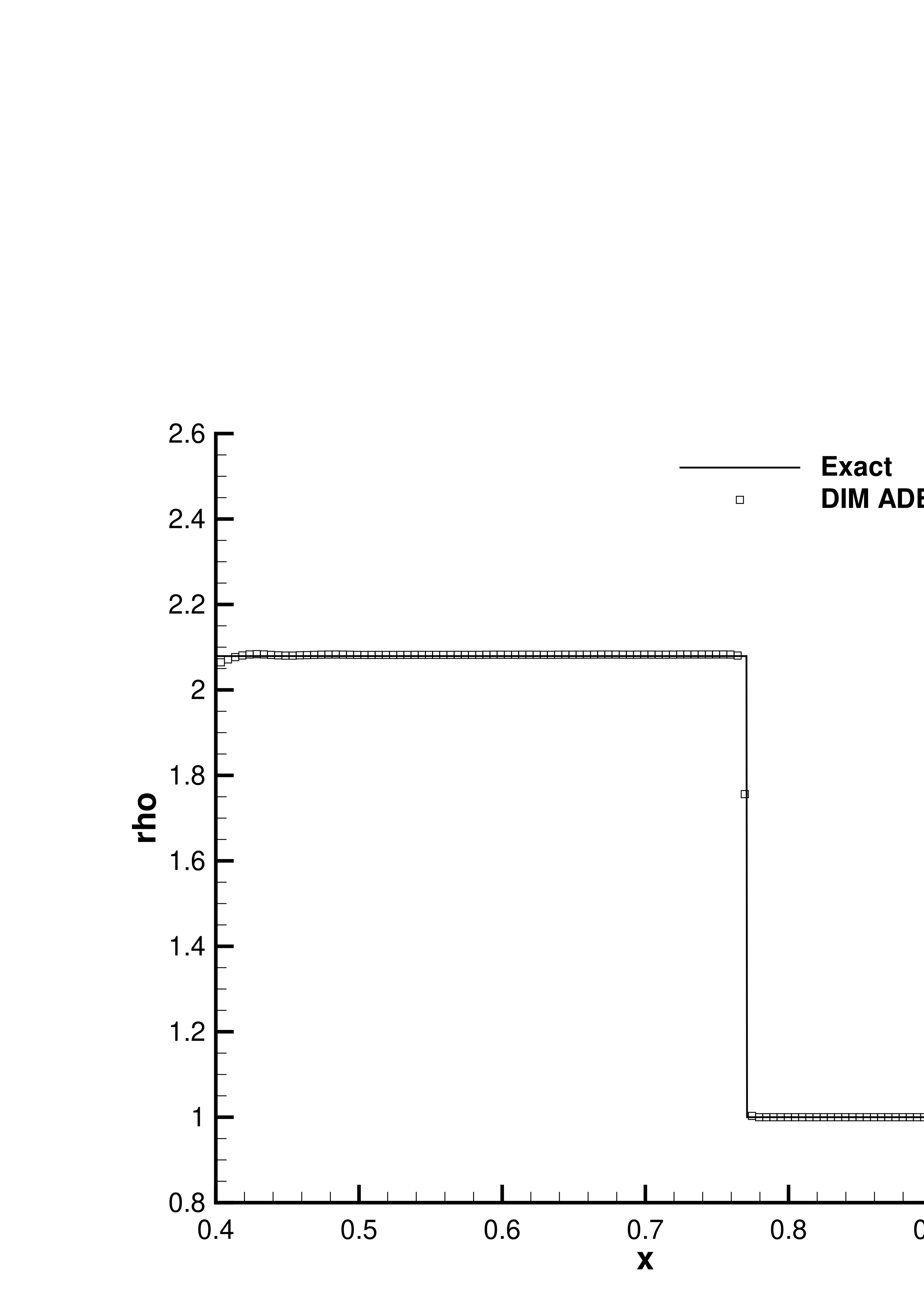
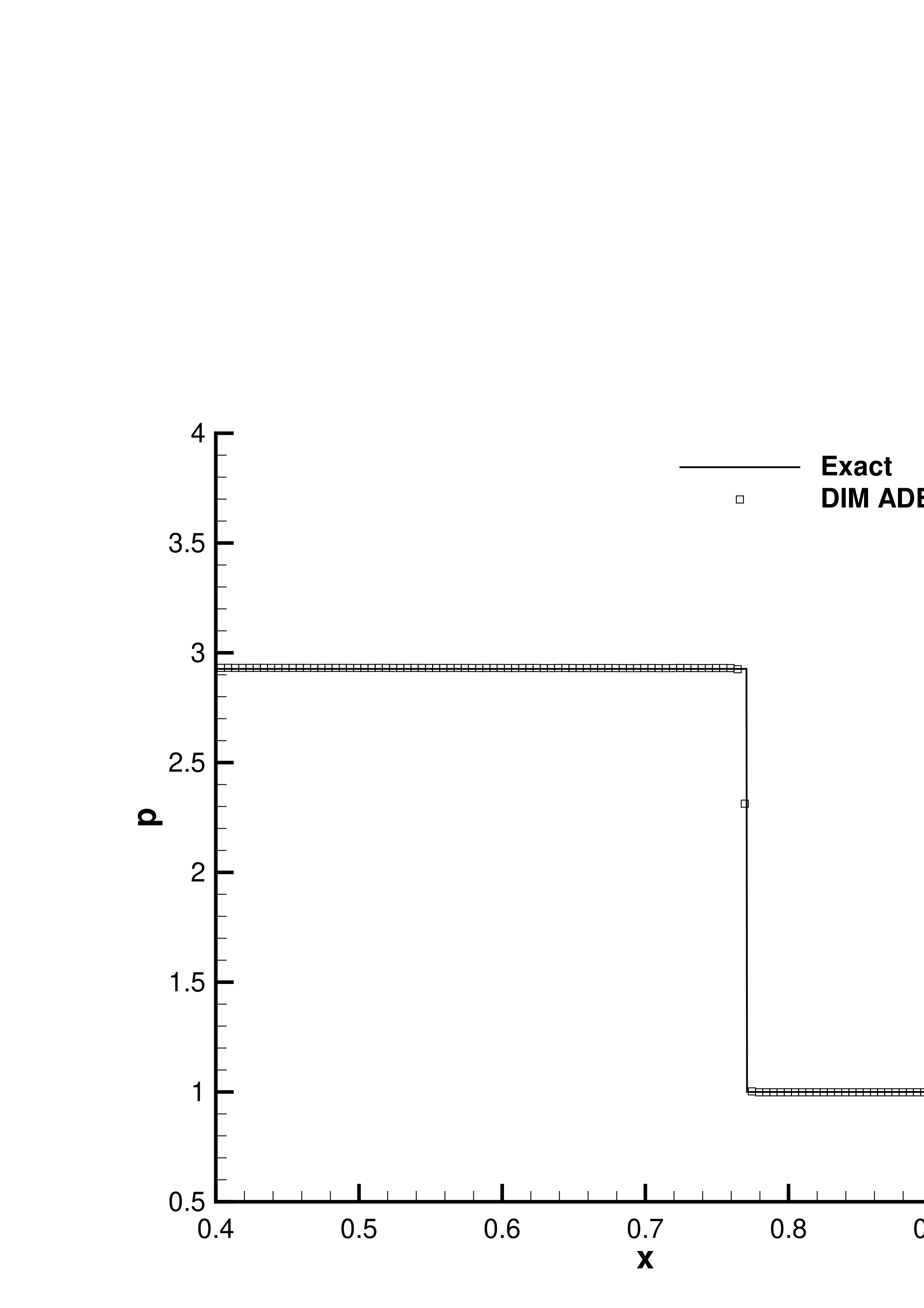
Figure 1: Riemann problem RP1 (slowly moving piston problem with shock wave) and comparison with the exact solution at time $t=0.4$. Fluid density (left), fluid velocity (center) and fluid pressure (right) in the volume occupied by the fluid.

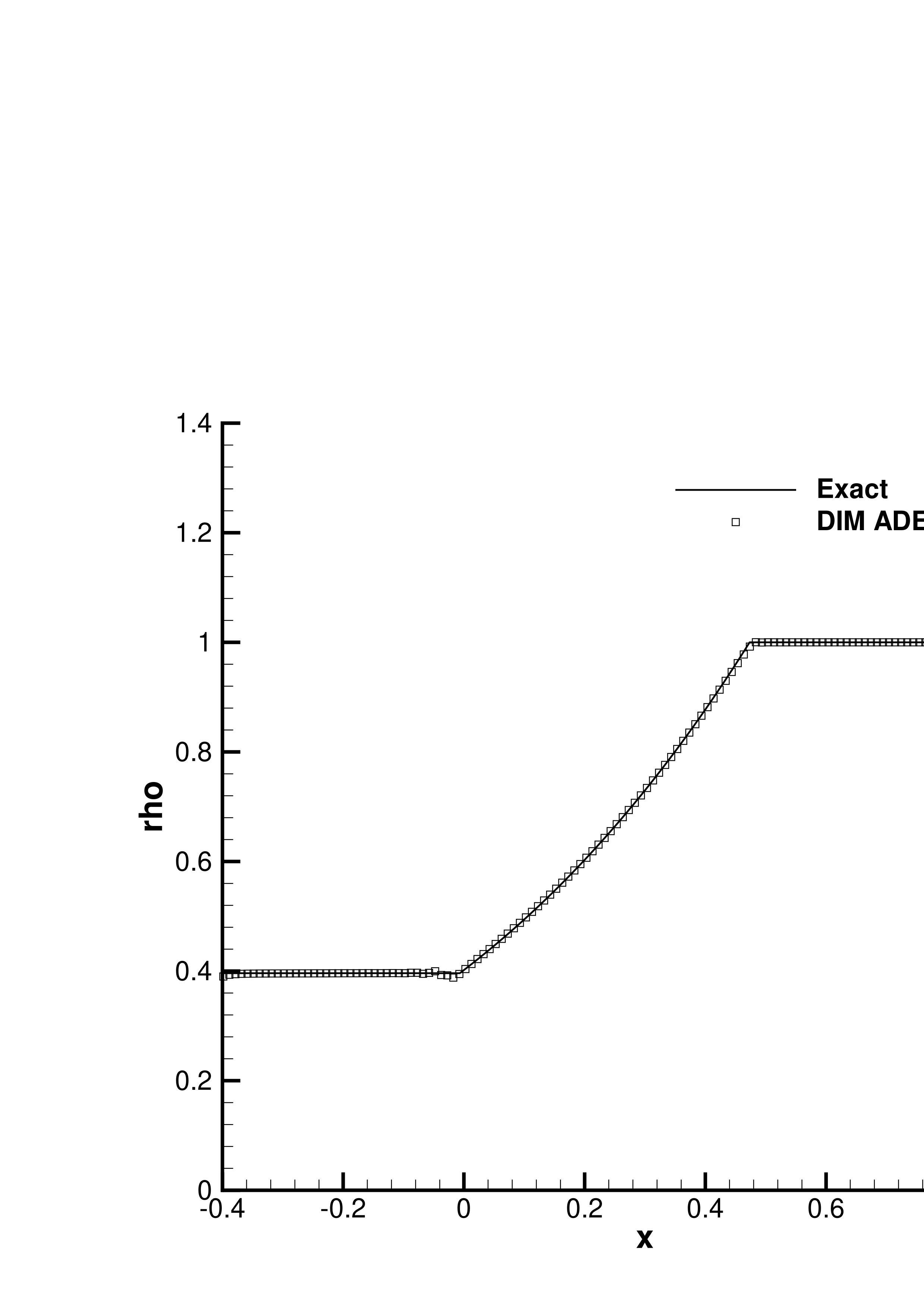
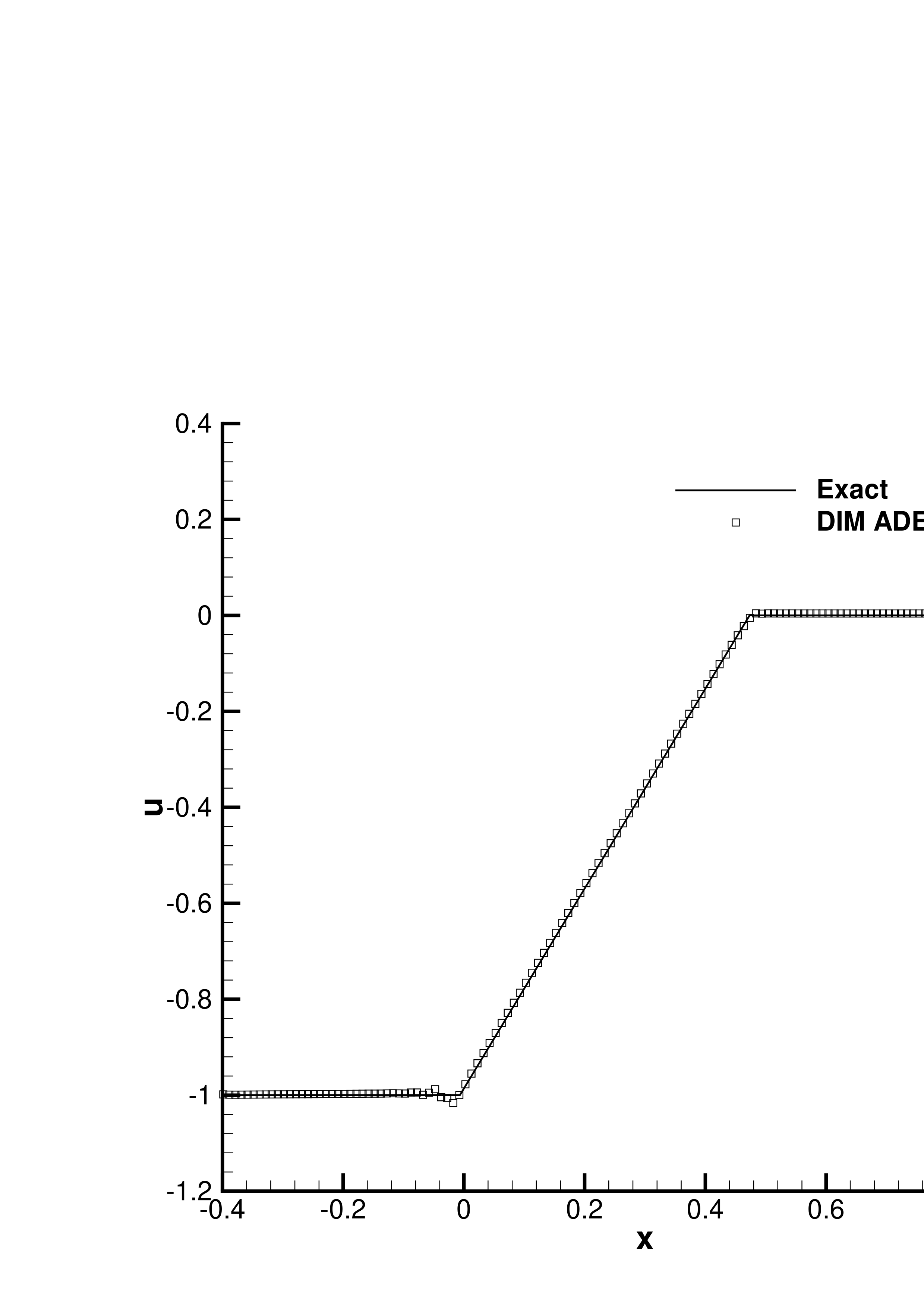
Figure 2: Riemann problem RP2 (moving piston problem with rarefaction) and comparison with the exact solution at time $t=0.4$. Fluid density (left), fluid velocity (center) and fluid pressure (right) in the volume occupied by the fluid.

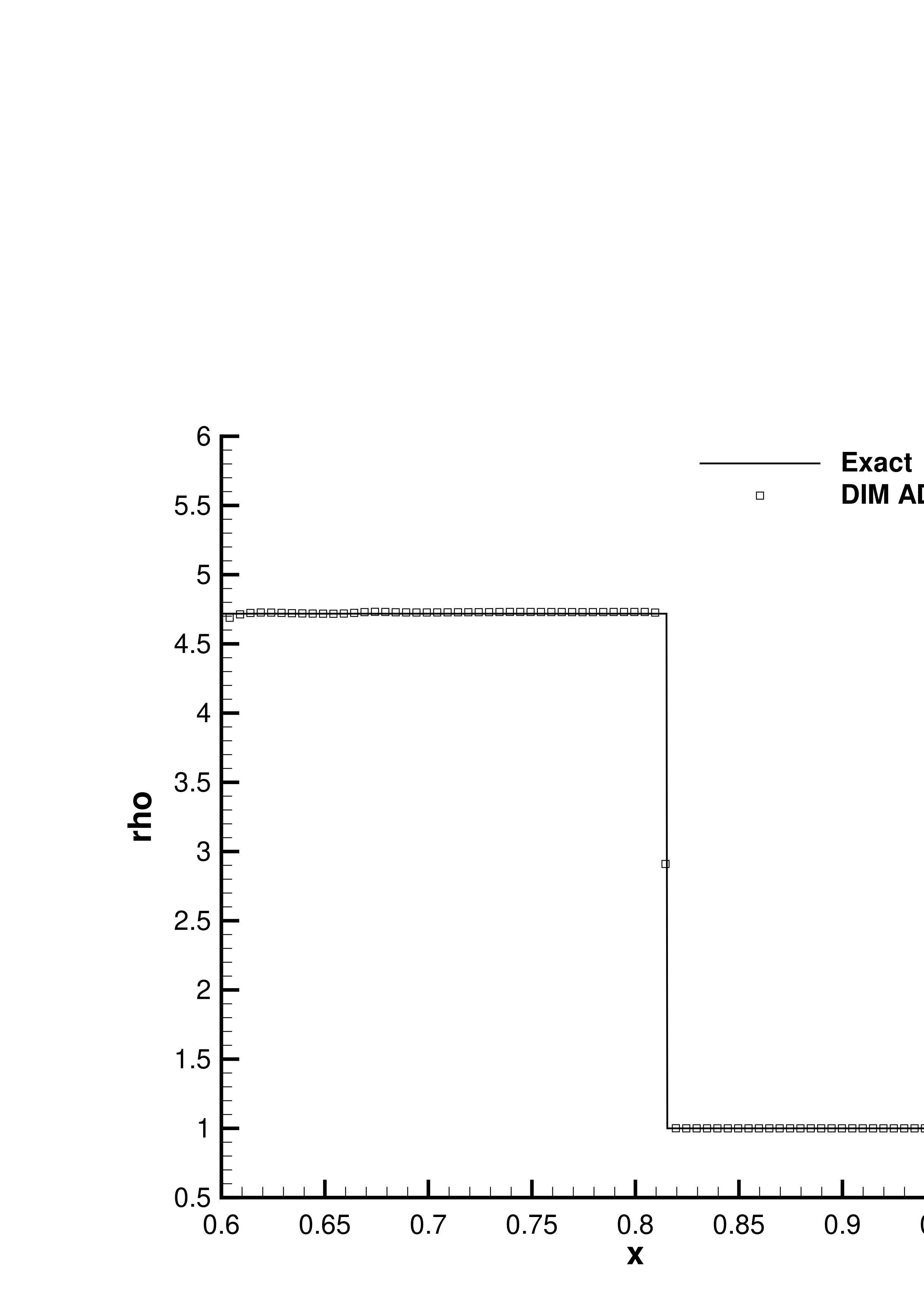
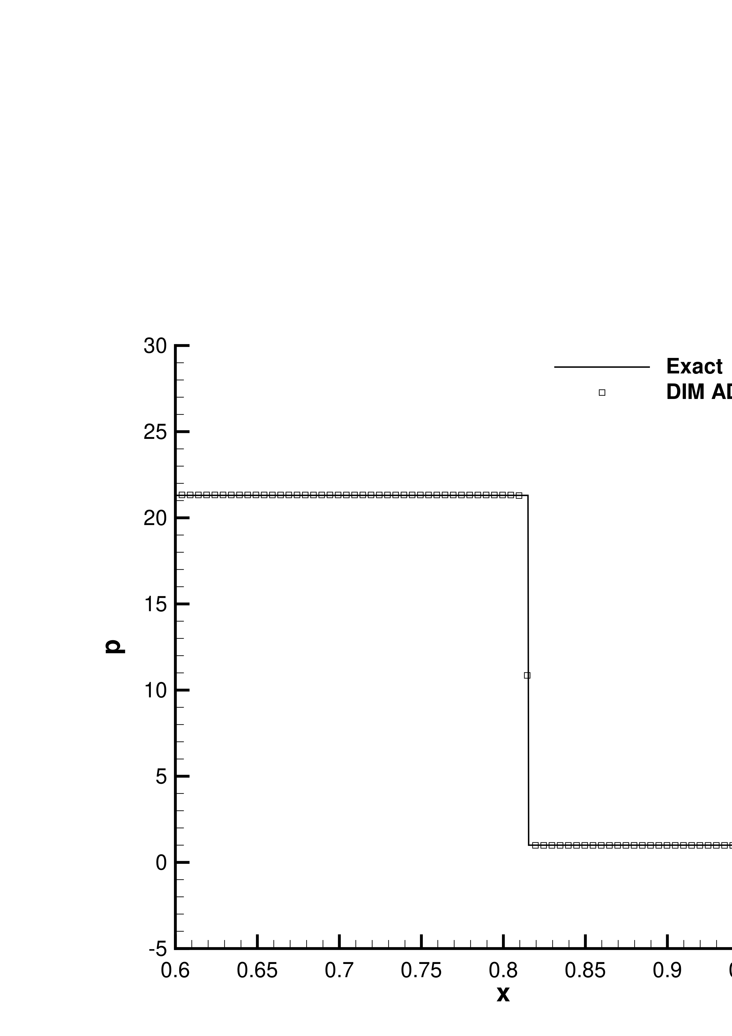
Figure 3: Riemann problem RP3 (fast moving piston problem with shock wave) and comparison with the exact solution at time $t=0.2$. Fluid density (left), fluid velocity (center) and fluid pressure (right) in the volume occupied by the fluid.

4.2 Single Mach reflection

Here we solve the singe Mach reflection problem proposed in [134] and for which experimental reference data in form of Schlieren images are available in [134] and [139]. The test consists of a shock wave initially located in $x=0$ and traveling at shock Mach number of $M=1.7$ to the right, where it is hitting a wedge of angle $\varphi=25^{\circ}$. The upstream density and pressure in front of the shock ($x>0$) are $\rho_{0}=1$ and $p_{0}=1/\gamma_{g}$, respectively. Ahead of the shock, the fluid is at rest ($\mathbf{v}_{0}=0$). The post-shock values for $x<0$ can then be computed via the standard Rankine-Hugoniot conditions of the compressible Euler equations.

The computational domain is $\Omega=[0,3]\times[0,2]$ and is discretized using $100\times 50$ ADER-DG elements of degree $N=5$. The initial volume fraction function is chosen as $\alpha=\varepsilon$ for $y<\tan(\varphi)\,x$ and $\alpha=1-\varepsilon$ elsewhere. The velocity of the solid is set to $\mathbf{v}_{s}=0$. The simulation is run until $t=1.2$ and the obtained computational results are summarized in Figure 4. The obtained flow field agrees very well with the reference solution shown in [134]. The shock is in the right location and is well resolved with our high order scheme, although only a very coarse mesh has been used. The limiter is activated along the fluid-solid interface, and along the impinging and reflected shock waves. We emphasize again that all that is needed in order to represent the geometry of the rigid solid body is to set the volume fraction function $\alpha$ to a small positive value inside the solid, and to almost unity outside.

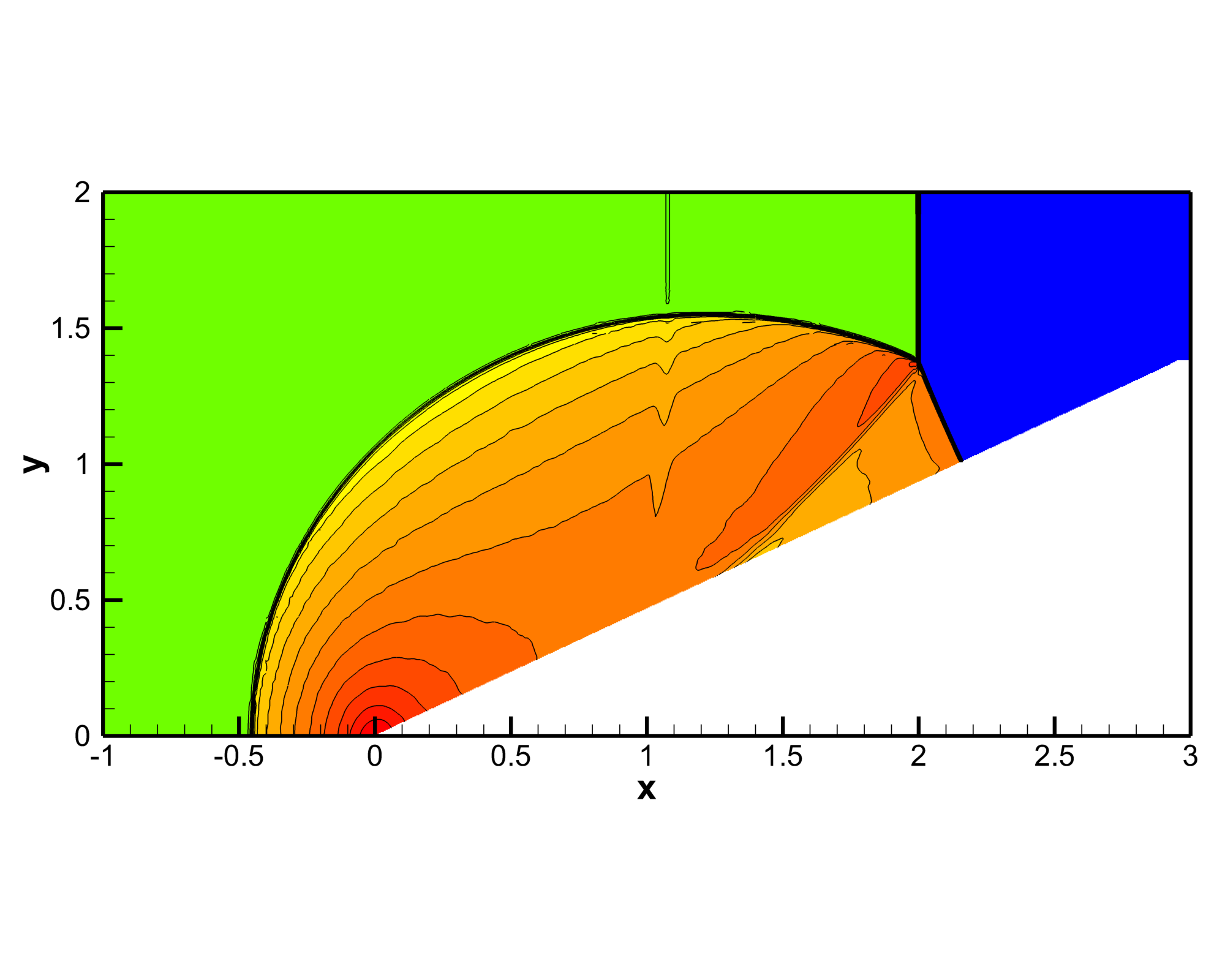
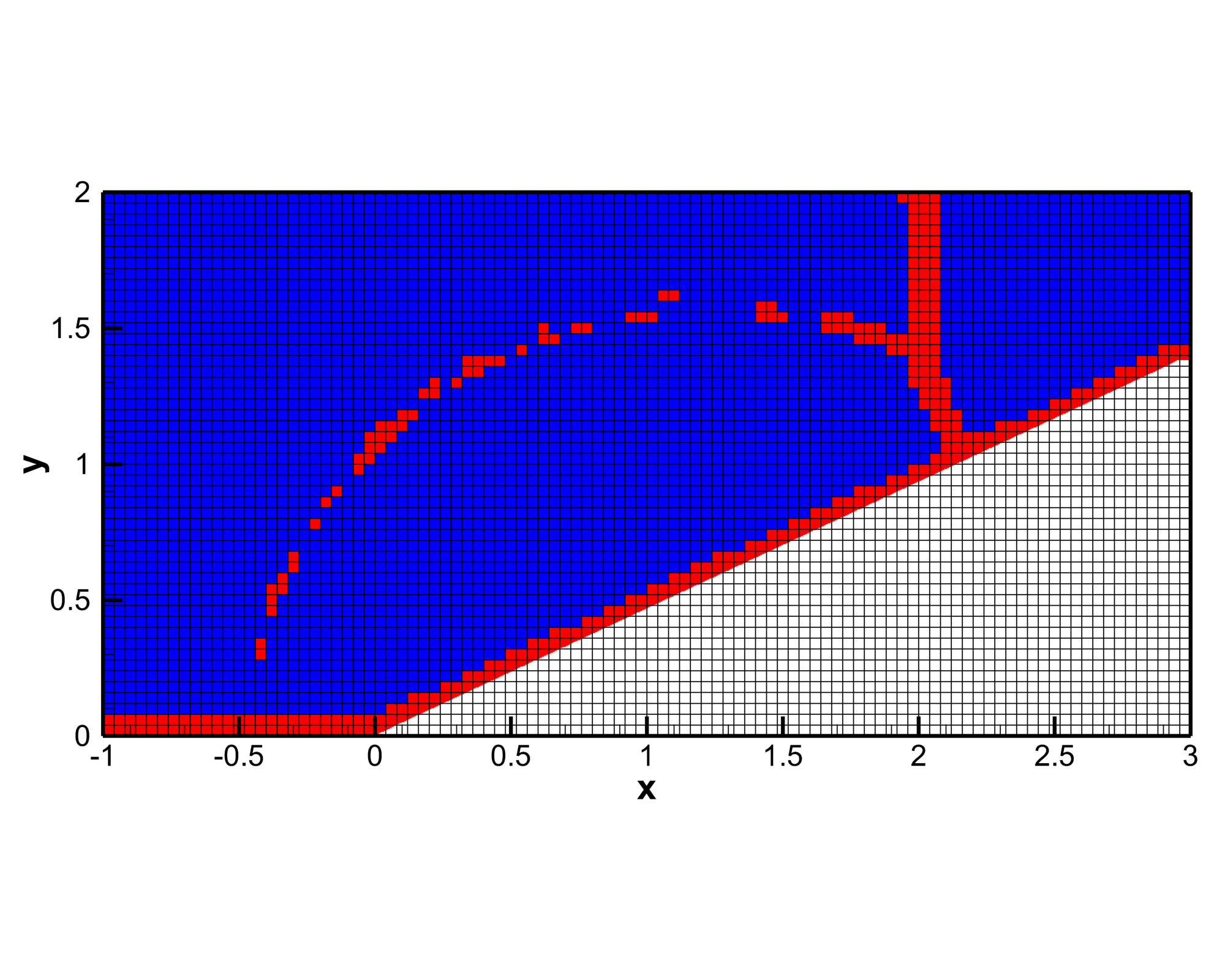
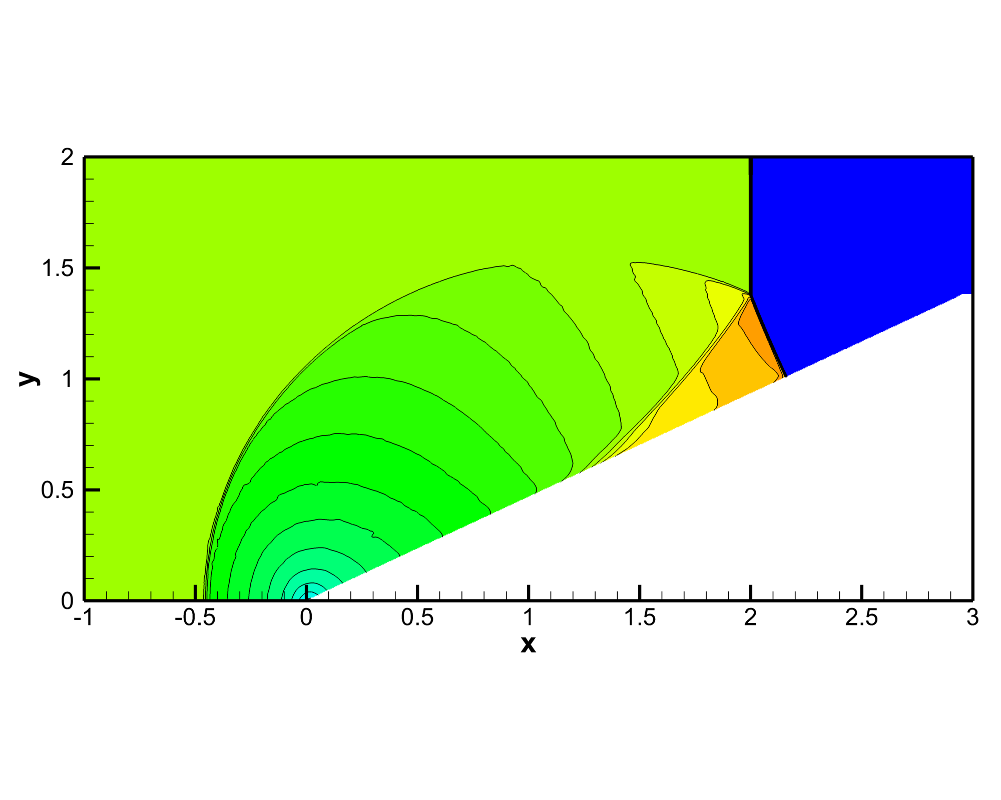
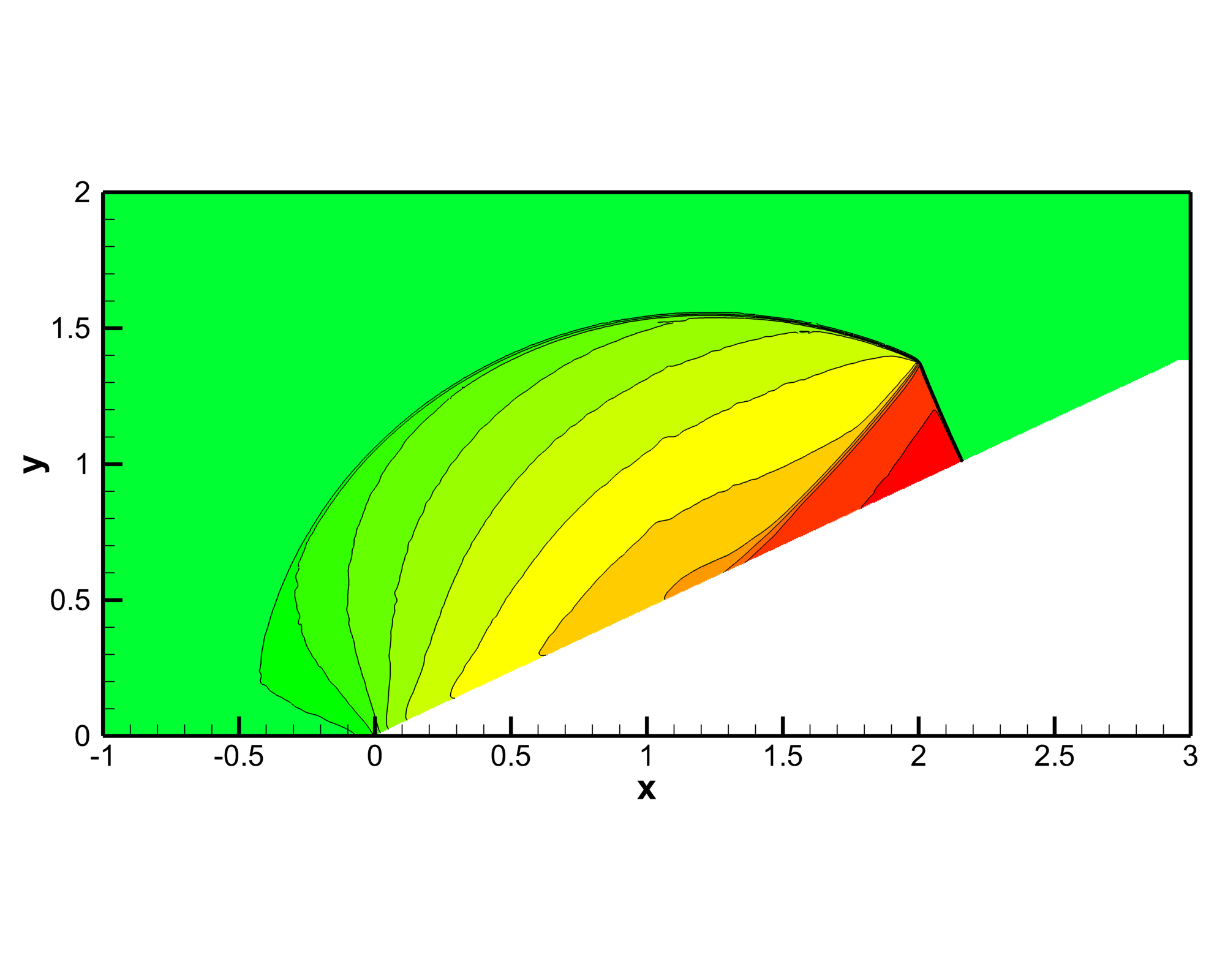
Figure 4: Single Mach reflection problem at time $t=1.2$ using an ADER-DG scheme with $N=5$ and a posteriori sub-cell FV limiter. Density contour colors (top left), limiter map and computational mesh (top right), velocity component $u$ (bottom left) and velocity component $v$ (bottom right).

4.3 Flow of a shock over a wedge

Here we solve a similar problem as before by considering the interaction of a mild shock wave with a two dimensional wedge. For this test, experimental reference data are again available under the form of Schlieren photographs, see [139, 125, 39].

The computational domain is $\Omega=[-2,6]\times[-3,3]$ and is discretized with $200\times 150$ ADER-DG elements with polynomial approximation degree $N=5$. The scheme is supplemented with a posteriori sub-cell finite volume limiter. The tip of a wedge with length $L=1$ and height $H=1$ is placed at $x=0$. Inside the wedge we set the initial volume fraction function to $\alpha=\varepsilon$, and outside we use $\alpha=1-\varepsilon$, with $\varepsilon=10^{-2}$. In the gas, the exact solution of a shock wave of shock Mach number $M_{s}=1.3$ is setup via the Rankine-Hugoniot conditions of the compressible Euler equations. In front of the shock, the fluid is at rest and has a density of $\rho=1.4$ and a pressure of $p=1$. The solid velocity is set to $\mathbf{v}_{s}=0$ everywhere.

The computational results are depicted in Figure 5. Comparing our results qualitatively with the Schlieren images produced by Schardin [125], we note an excellent agreement. All the reflected and refracted waves as well as the vortices shed from the wedge are resolved correctly. Our set of images corresponds to pictures 2, 5, 8 and 17 shown in [125]. For a numerical reference solution obtained with high order ADER-FV schemes on a very fine boundary-fitted unstructured triangular mesh, see [39].

Again, this rather complex flow field is simply produced via a spatially variable volume fraction function $\alpha$, which defines the geometry of the obstacle. In principle, with our new approach obstacles of arbitrary shape could be described.

The temporal evolution of the limiter is shown in Figure 6. The limiter is activated on the fluid-solid interface and on the main shock wave, as expected.

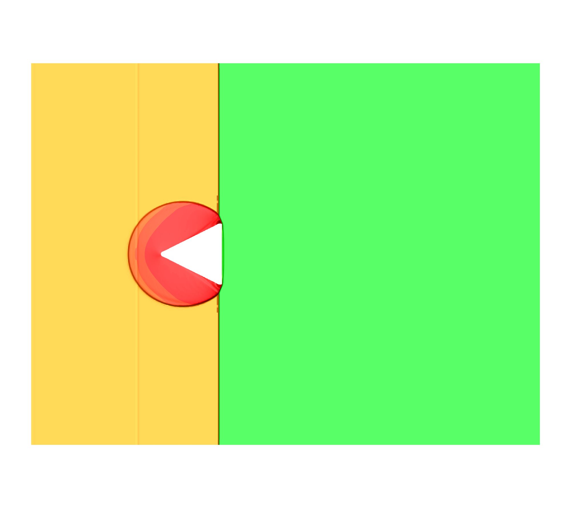
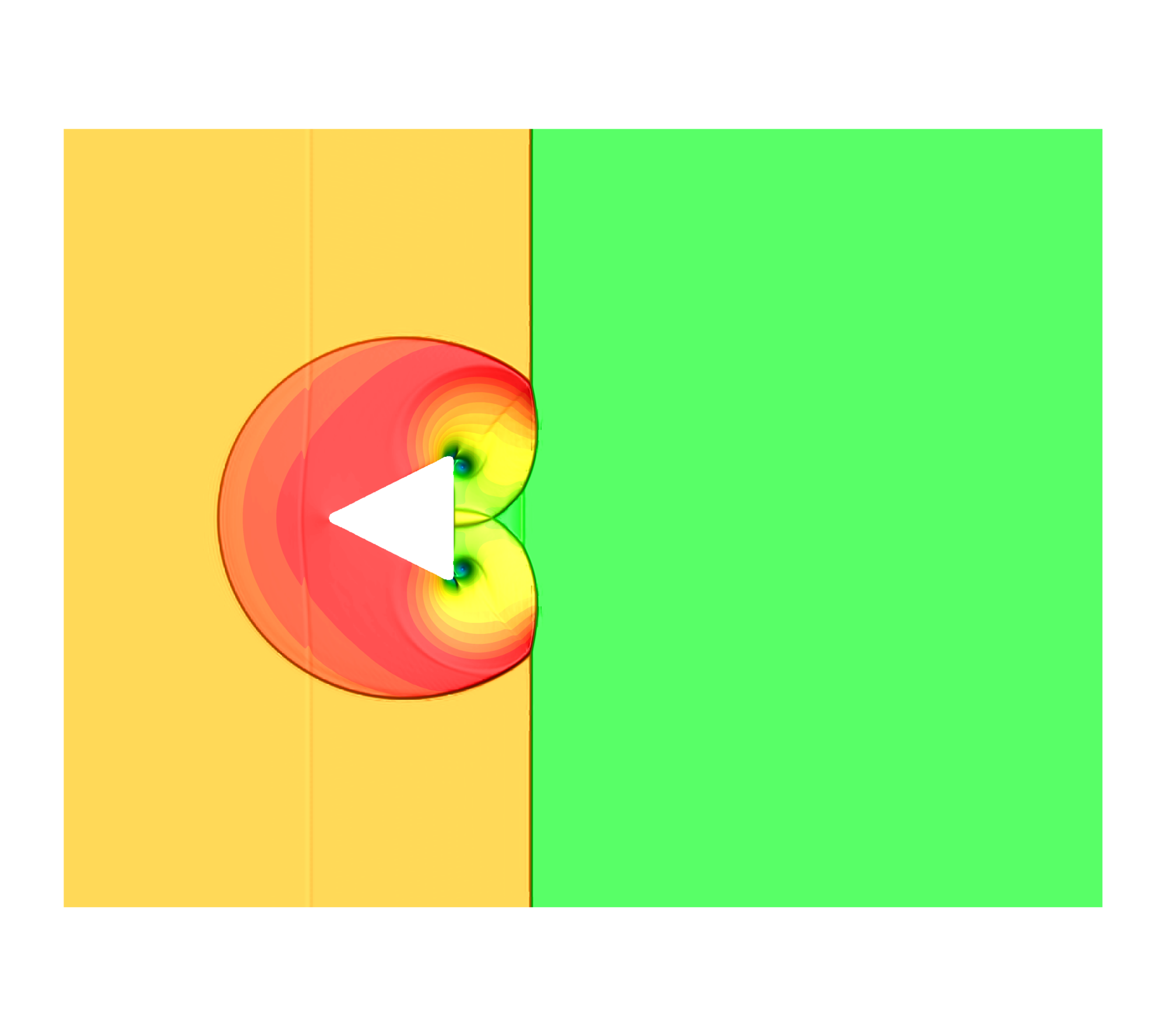
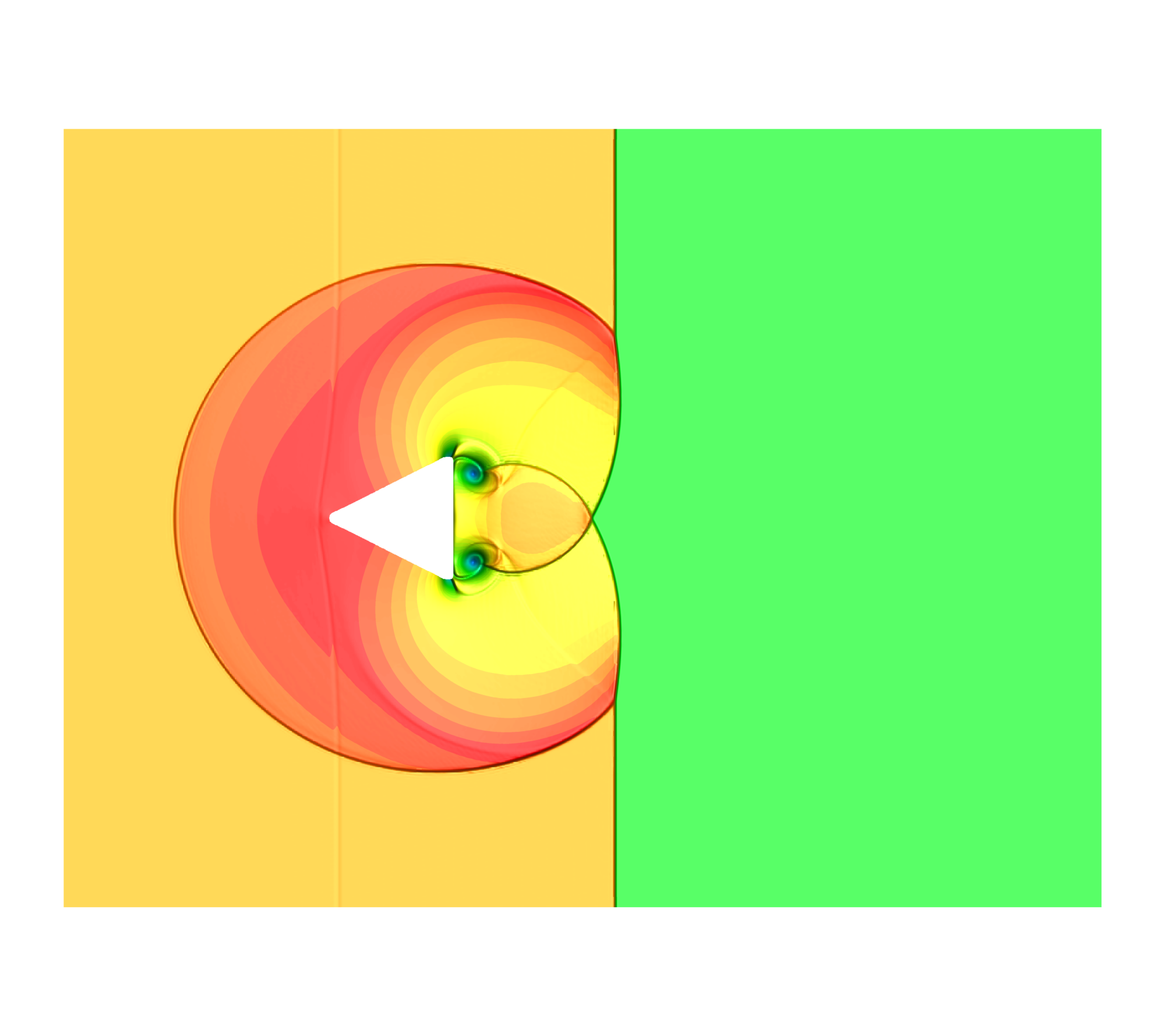
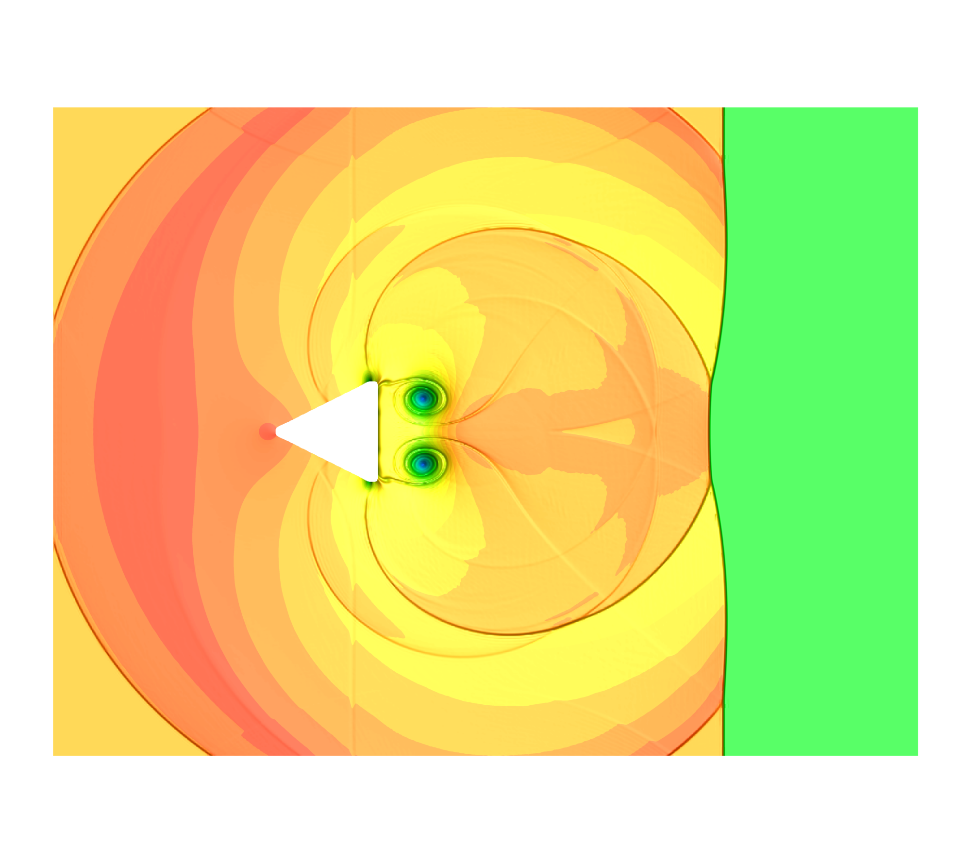
Figure 5: Density contours obtained with the diffuse interface model for the shock-wedge interaction problem using a sixth order ADER-DG scheme with a posteriori sub-cell finite volume limiter. Output times from top left to bottom right: $t=1.5$, $t=2.0$, $t=2.5$, $t=4.0$.

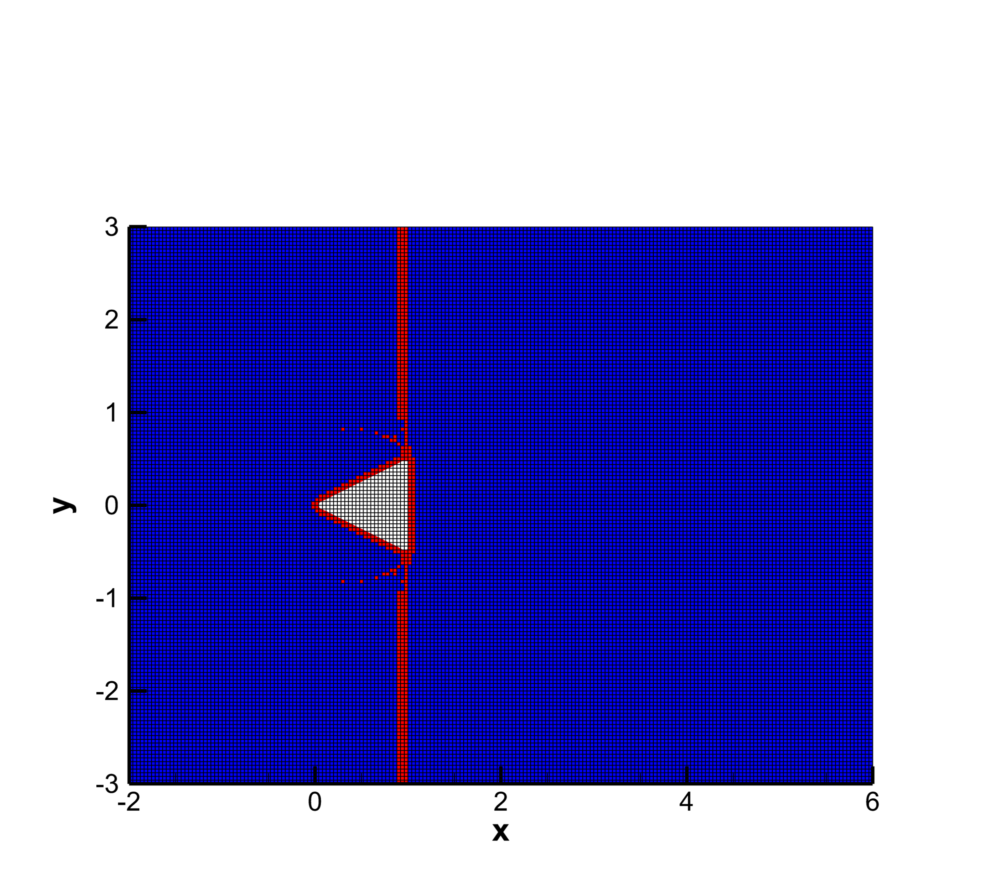
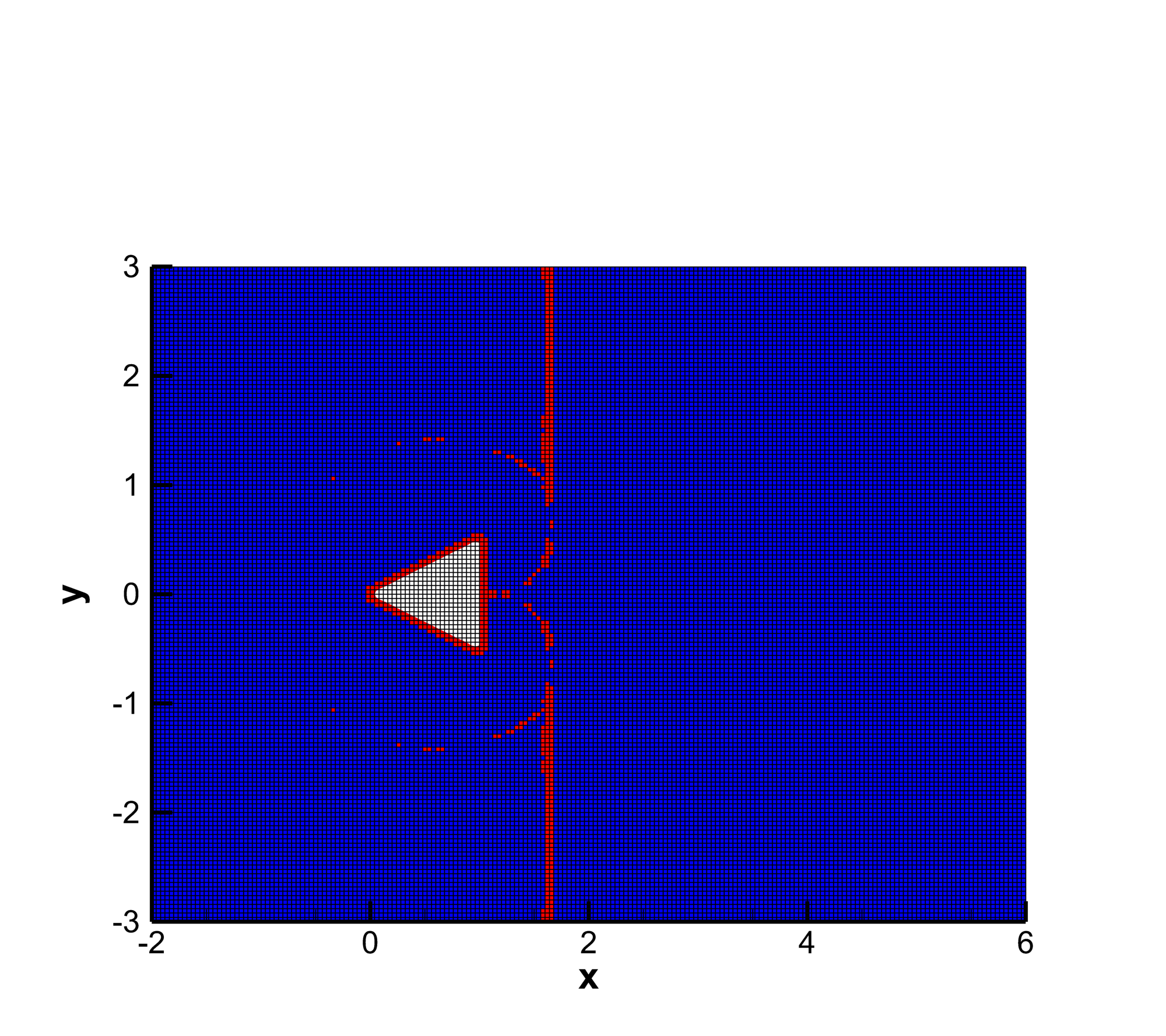
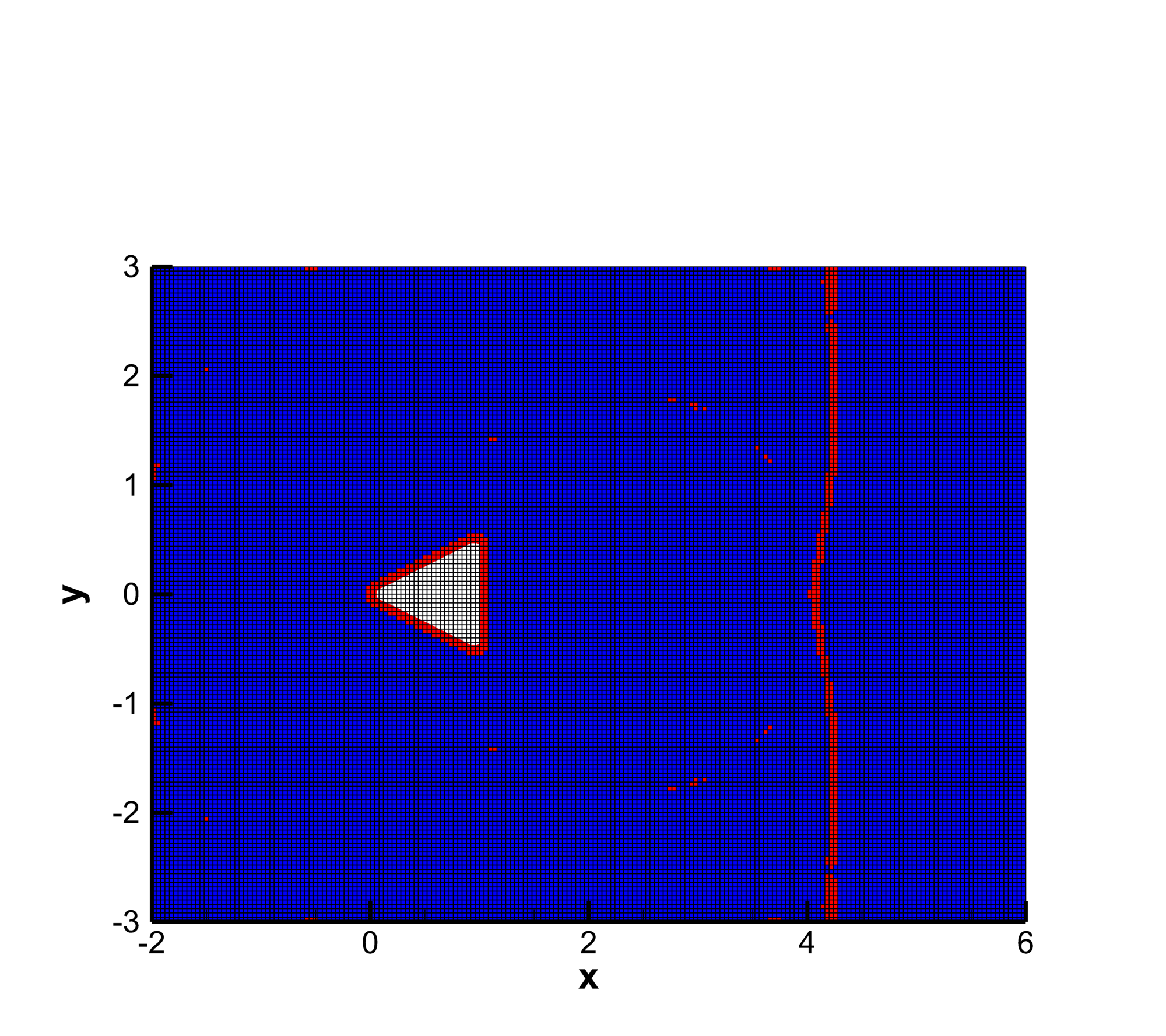
Figure 6: Limiter map for the shock-wedge interaction problem using a sixth order ADER-DG scheme with a posteriori sub-cell finite volume limiter. Blue cells are unlimited, while red cells have been flagged as troubled. Output times from top left to bottom right: $t=1.5$, $t=2.0$, $t=2.5$, $t=4.0$.

4.4 Mach 3 flow over a blunt body

The next example concerns a supersonic flow with Mach number $M=3$ over a circular cylinder. The two-dimensional computational domain is $\Omega=[-1,0]\times[-1,+1]$, which is discretized using $100\times 200$ ADER-DG elements of polynomial approximation degree $N=5$ and a posteriori sub-cell finite volume limiter. The initial condition for the volume fraction function is simply chosen as follows: inside a circular cylinder of radius $R=0.5$ we set $\alpha=\varepsilon$ for $\left\|\mathbf{x}\right\|\leq 0.5$, while outside the cylinder, we set $\alpha=1-\varepsilon$ in the rest of the computational domain. Here, we use $\varepsilon=10^{-2}$. All other flow quantities are then simply initialized with the following constant values: $\rho=1.4$, $u=3$, $v=0$, $p=1$, $u_{s}=0$ and $v_{s}=0$. The computational results obtained at time $t=1$ are depicted in Figure 7. The typical detached bow shock ahead of the blunt body is formed. In the right panel of the same Figure, we also show the limiter map, where red elements are flagged as troubled, while blue cells indicate unlimited elements. One can not only easily see that the a posteriori MOOD algorithm is able to detect the shock wave properly, but also that our very high order scheme is able to resolve the geometry of the blunt body and the shock wave very well, despite using a very coarse mesh. Thanks to the subcell FV limiter, the interface can typically be resolved within one to two elements of the DG scheme, see right panel in Figure 7. In the limiter map one can observe some false positive activations of the limiter in the smooth subsonic area behind the bow shock. However, these local effects do not reduce the overall quality of the simulation. Since the entire scheme is nonlinear and no special care about symmetry preservation was made, such false positive activations can be non-symmetric and can be triggered either via spurious numerical oscillations, accumulated roundoff errors or by passing acoustic waves. The main flow field, however, remains essentially symmetric w.r.t. the $x$ axis.

We stress again that also in this test case the entire flow field and the bow shock are merely generated by the spatially varying volume fraction function, which is the only information that is needed in order to represent the geometry of the solid body.

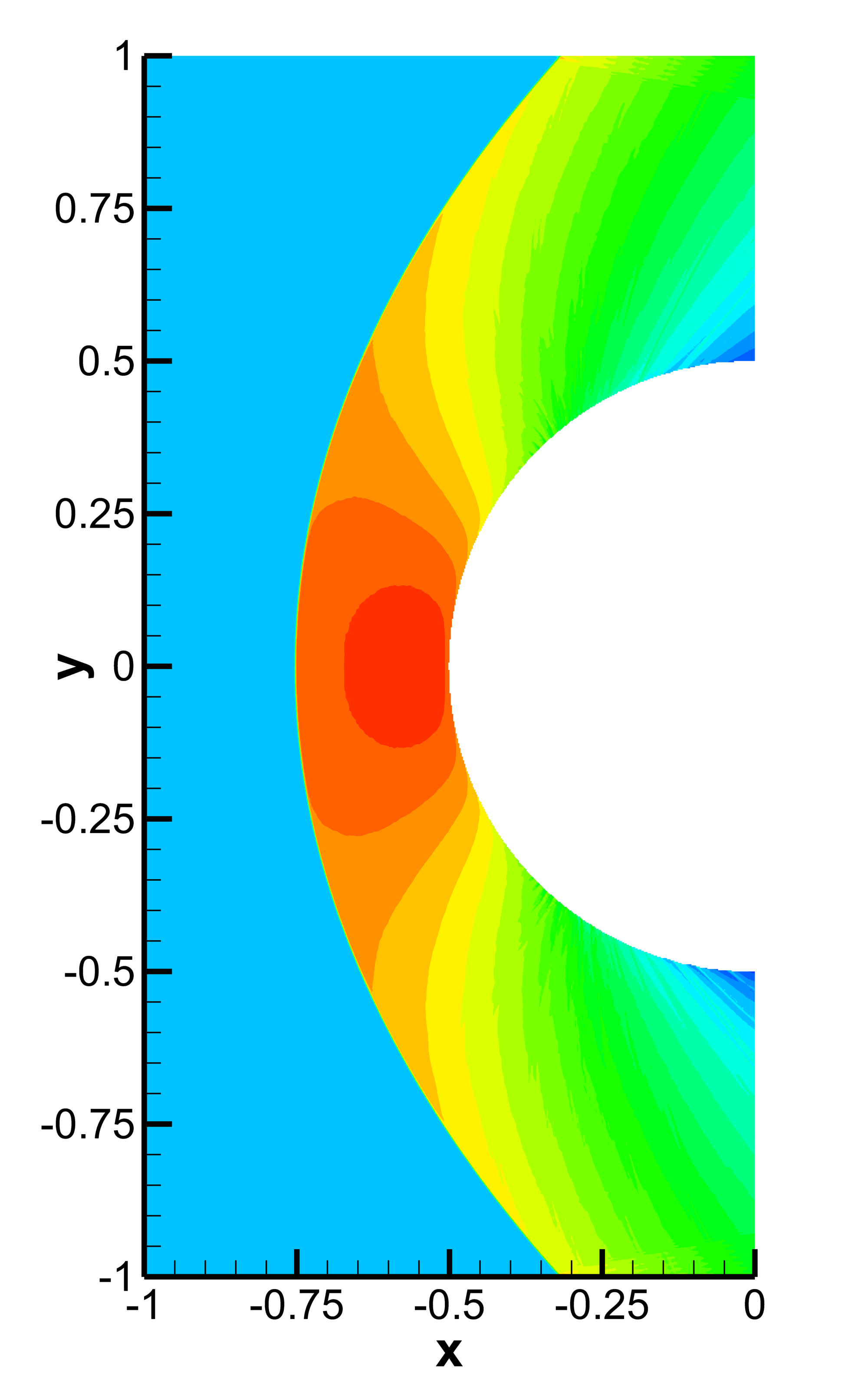
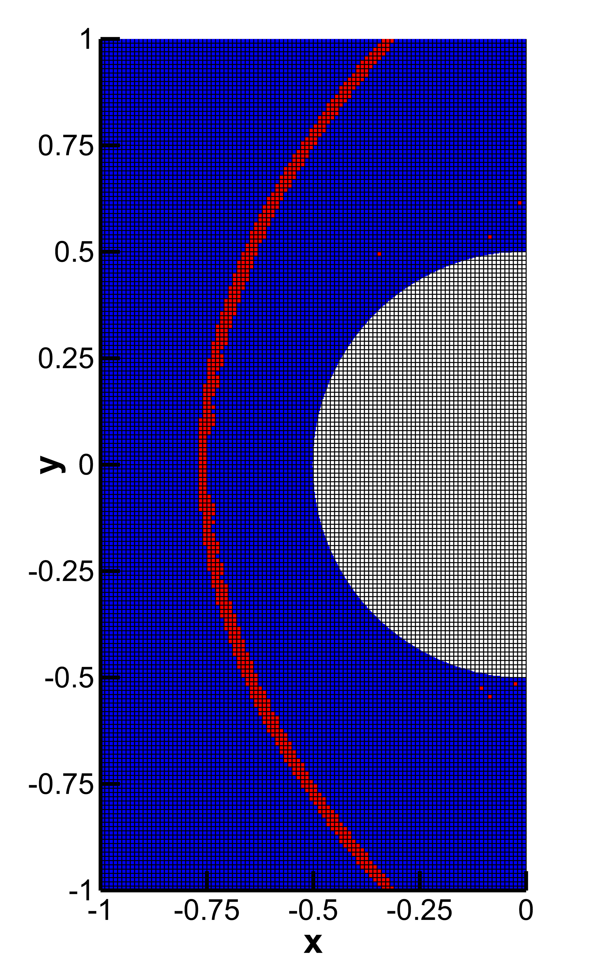
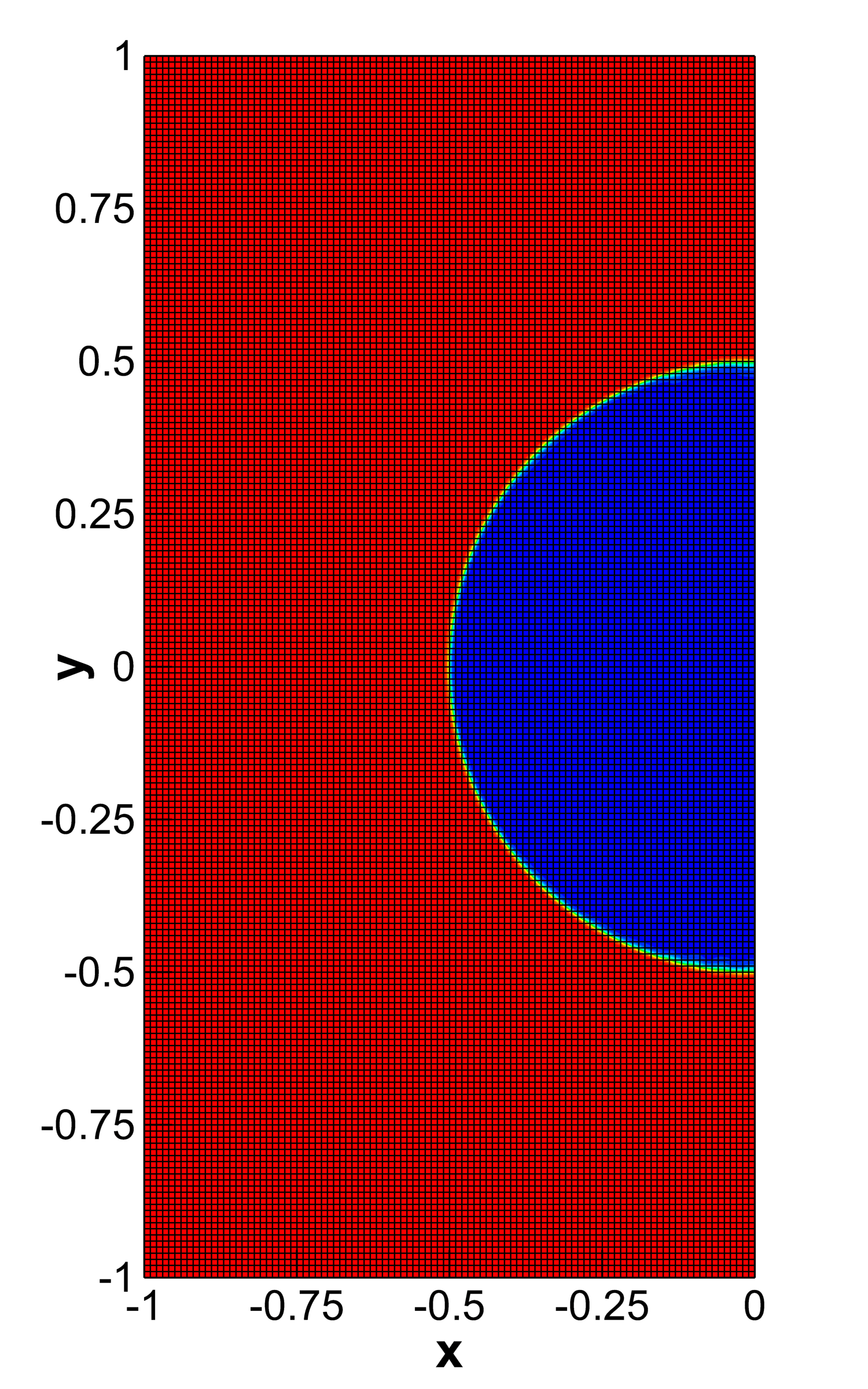
Figure 7: Supersonic flow over a blunt body with Mach number $M=3$ at time $t=1$ using an ADER-DG scheme with $N=5$ and a posteriori sub-cell finite volume limiter. Density contour colors (left) and limiter map with uniform Cartesian grid (center). Only cells with $\alpha>0.5$ are shown in the left and center panel. Equidistant alpha contour colors (right). The interface is typically resolved within one or two grid cells.

4.5 Three cylinders rotating in a compressible gas at supersonic speed

This last example is only meant to be a showcase to illustrate the applicability of the diffuse interface model proposed in this paper. We choose the computational domain $\Omega=[-2,+2]\times[-2,+2]$, which is discretized with a Cartesian grid of $100\times 100$ equidistant ADER-DG elements. The polynomial degree of the basis functions is chosen as $N=3$. Periodic boundary conditions are applied everywhere. The initial condition for the fluid is $\rho=1.4$, $\mathbf{v}=0$ and $p=1$, while the solid velocity is initialized as a rigid body rotation with $\mathbf{v}_{s}=\bm{\omega}\times\mathbf{x}$, with $\bm{\omega}=(0,0,-3)$. We consider three circular solid bodies of radius $R_{c}=0.2$, whose centers $\mathbf{x}_{i}$ are initially located on a circle of radius $R_{0}$, i.e. $\mathbf{x}_{i}=R_{0}\left(\cos(\varphi_{i}),\sin(\varphi_{i})\right)$ with $\varphi_{i}=\frac{i}{3}\cdot 2\pi$. With this configuration, the centers of the circles move at a supersonic Mach number of $M=3$. The entire test problem is setup by simply defining the solid velocity field and by setting inside each circular solid body $\alpha=\varepsilon$, while in the rest of the domain, we choose $\alpha=1-\varepsilon$, with $\varepsilon=10^{-3}$. Nothing else needs to be done. Simulations are carried out until $t=2.0$. The density contour colors at different output times are depicted in Figure 8, where we have blanked regions where $\alpha<0.5$. One can clearly see the wake generated behind each cylinder, as well as the bow shock in front of each cylinder. At later times, the wakes and the bow shocks of two consecutive cylinders interact with each other. In order to assess the level of numerical diffusion present in the volume fraction function $\alpha$, we also show the temporal evolution of $\alpha$ in Figure 9. It can be seen that the interface is resolved within 3-4 DG cells, which is much more than in the case of the stationary blunt body shown in the previous section. In this context, less dissipative Riemann solvers, such as those forwarded in [43, 33], and better slope limiters [134] need to be used in the future, also in combination with AMR [44, 141].

One last time we stress that the entire setup of this test problem is very simple and that this very complex flow field and the description of the moving solid bodies is directly done inside the PDE system and only by prescribing a simple scalar volume fraction function. No moving body-fitted mesh needs to be generated.

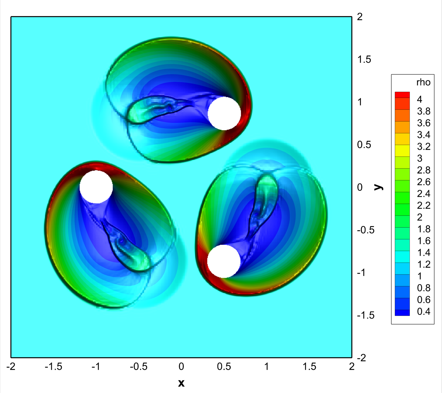
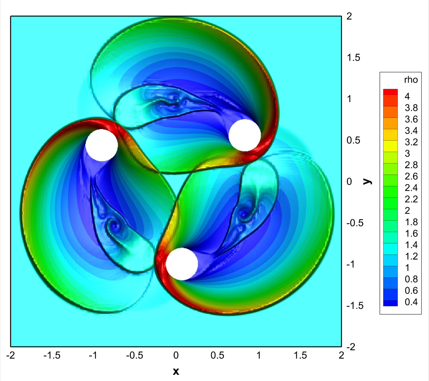
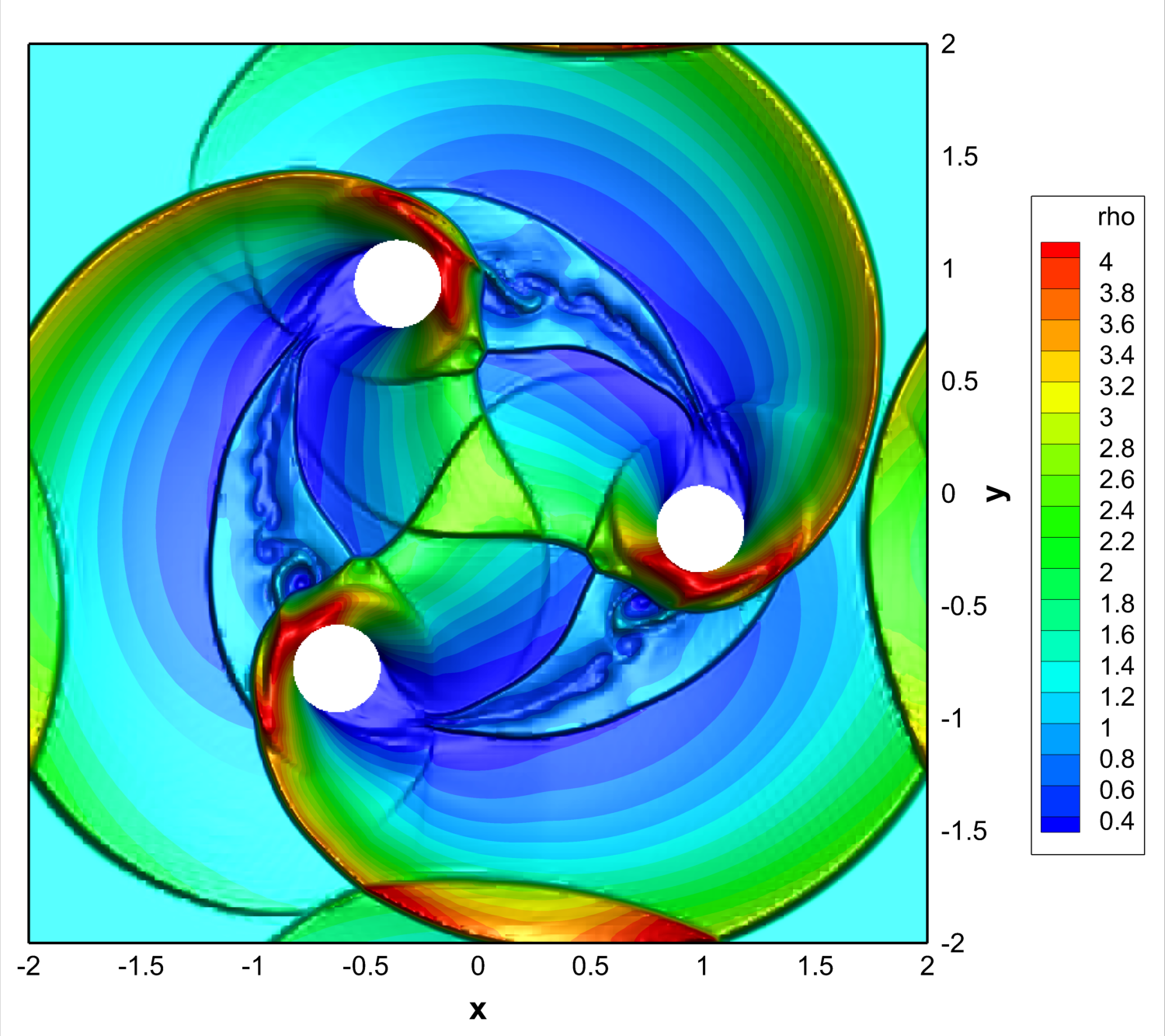
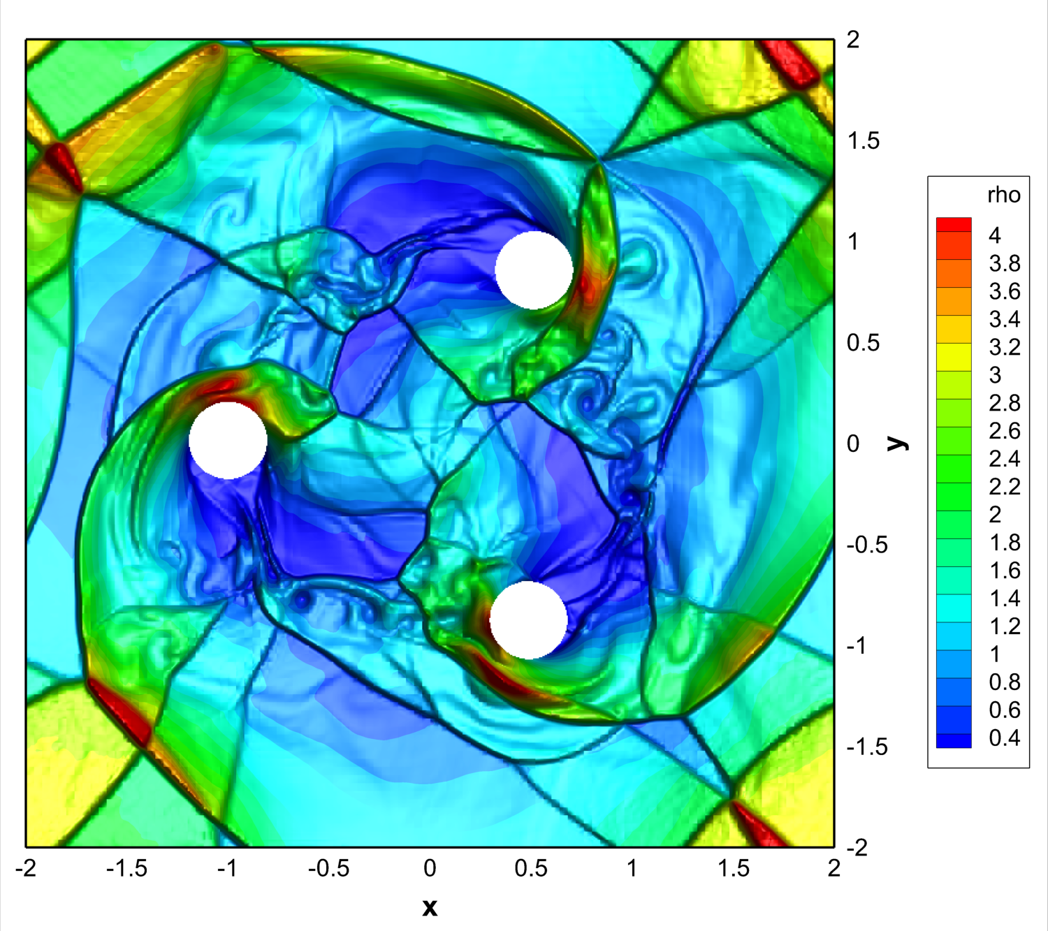
Figure 8: Three cylinders rotating at supersonic speed in a compressible gas. Output times from top left to bottom right: $t=0.35$, $t=0.5$, $t=0.75$ and $t=1.75$.

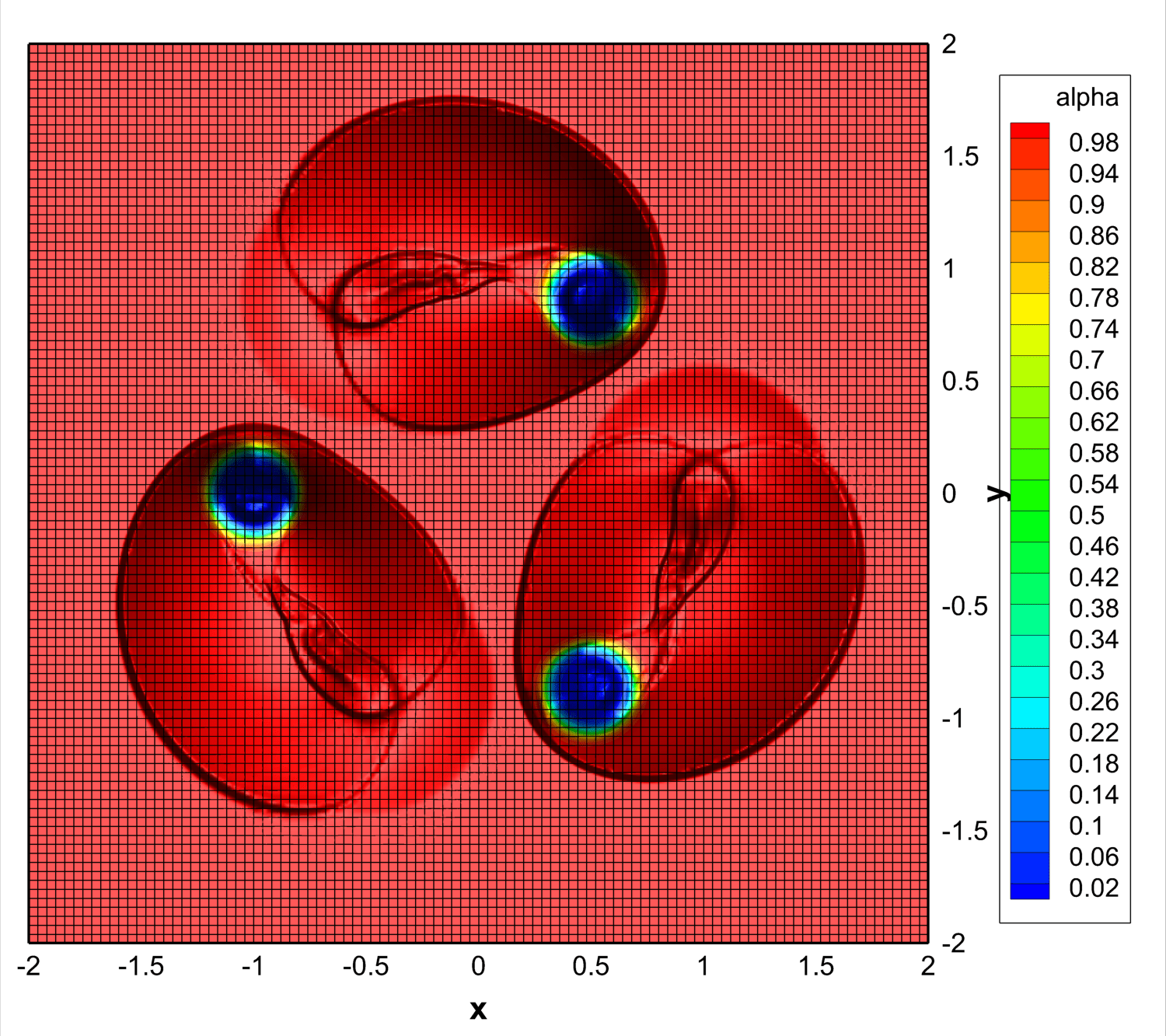
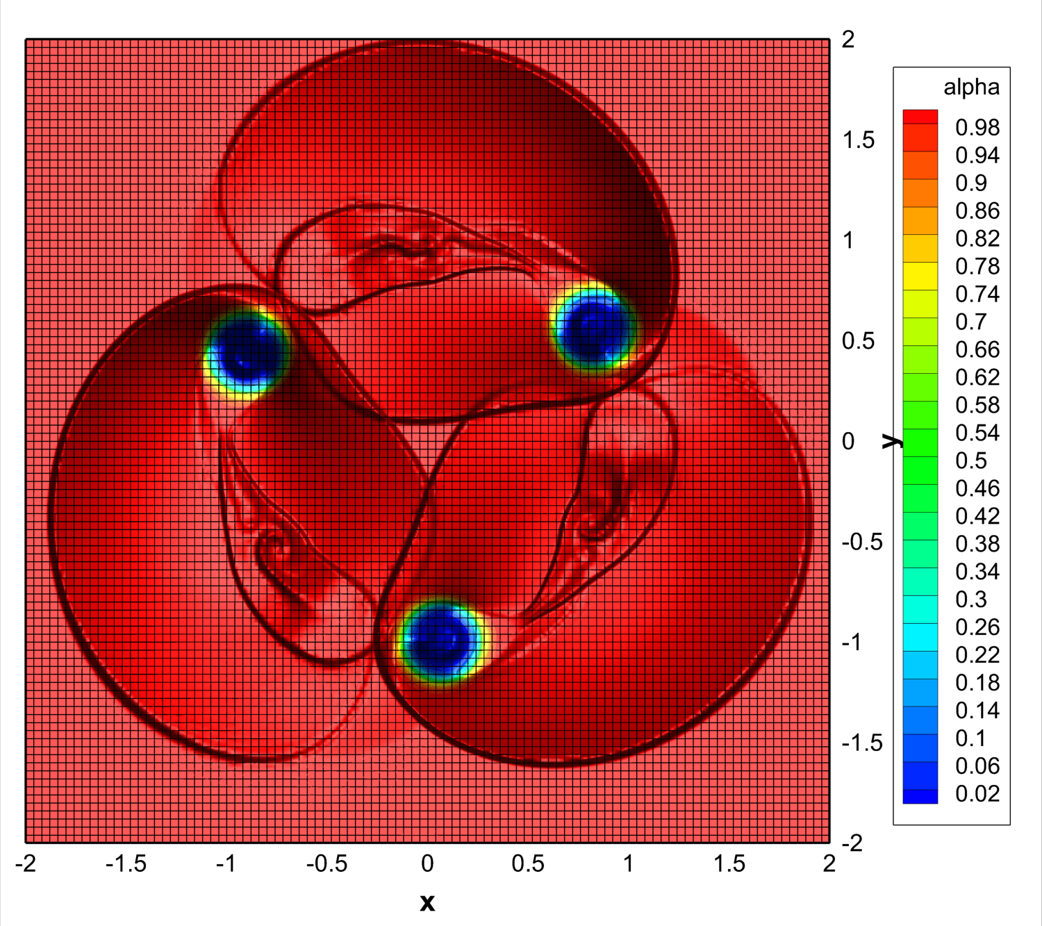
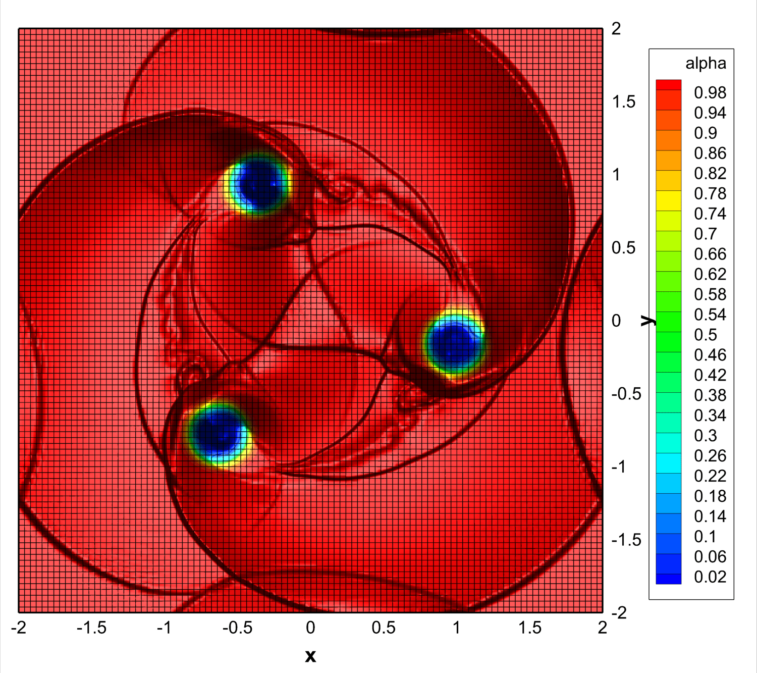
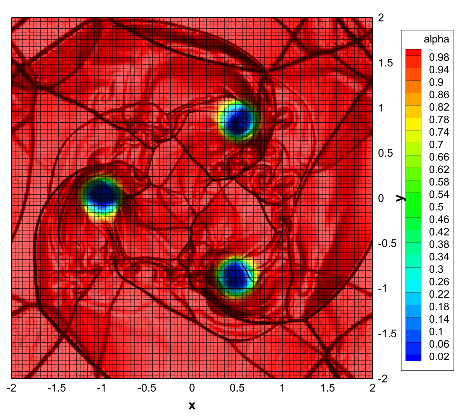
Figure 9: Volume fraction function $\alpha$ for the three cylinders rotating at supersonic speed in a compressible gas. Output times from top left to bottom right: $t=0.35$, $t=0.5$, $t=0.75$ and $t=1.75$.

5 Conclusion

In this paper we have introduced a new and very simple diffuse interface model for the simulation of compressible flows around fixed and moving rigid bodies of arbitrary shape. The proposed approach is so simple that all simulations can be carried out on uniform Cartesian grids. The geometry of each solid body is simply defined by a scalar volume fraction function, which assumes a value close to zero inside the solids and close to unity inside the compressible fluid. The computational setup can be done in a fully automatic manner, without the need to generate a body-fitted structured or unstructured mesh, which can become very time consuming for complex geometries. The work presented in this paper is a natural extension of the simple diffuse interface approach introduced in [30, 31, 59, 129] and [14]. The presented numerical algorithm with the underlying diffuse interface model is a consequent application of Godunov’s shock capturing ideas to the context of moving material interfaces. Rather than tracking the material interface via a moving mesh, one simply needs to evolve in time the additional scalar quantity $\alpha$, which contains all the necessary information about the geometry of the problem.

In the first part of this paper we have proven, via Riemann invariants and via generalized Rankine-Hugoniot conditions derived from the DLM theory [89], that the normal component of the fluid velocity at the material interface assumes automatically the value of the normal component of the solid velocity when the fluid volume fraction $\alpha$ jumps from unity to zero, i.e. the non-penetration boundary condition is naturally satisfied by the model. The proof based on generalized Rankine-Hugoniot conditions supposes a simple straight line segment path, which therefore also justifies its use inside path-conservative schemes, as those employed in this paper.

Future developments will concern the generalization to fluids interacting with elastic solids, via a combination of the compressible multi-phase model of Romenski et al. [118, 117, 116] and the equations of hyperelasticity in Euler coordinates of Godunov, Peshkov and Romenski (GPR model), forwarded in [65, 66, 108, 41, 42]. We also plan to include surface tension effects via the new hyperbolic surface tension model of Gavrilyuk et al., see [126, 20].

In memoriam

This paper is dedicated to the memory of Dr. Douglas Nelson Woods (^∗January 11^th 1985 - $\dagger$September 11^th 2019), promising young scientist and post-doctoral research fellow at Los Alamos National Laboratory. Our thoughts and wishes go to his wife Jessica, to his parents Susan and Tom, to his sister Rebecca and to his brother Chris, whom he left behind.

References

- [1] E. Abbate, A. Iollo, and G. Puppo. An asymptotic-preserving all-speed scheme for fluid dynamics and nonlinear elasticity. SIAM Journal on Scientific Computing, 41:A2850–A2879, 2019.
- [2] N. Andrianov, R. Saurel, and G. Warnecke. A simple method for compressible multiphase mixtures and interfaces. International Journal for Numerical Methods in Fluids, 41:109–131, 2003.
- [3] N. Andrianov and G. Warnecke. The Riemann problem for the Baer–Nunziato two-phase flow model. Journal of Computational Physics, 212:434–464, 2004.
- [4] M.R. Baer and J.W. Nunziato. A two-phase mixture theory for the deflagration-to-detonation transition (DDT) in reactive granular materials. J. Multiphase Flow, 12:861–889, 1986.
- [5] Philip T. Barton. An interface-capturing Godunov method for the simulation of compressible solid-fluid problems. Journal of Computational Physics, 390:25–50, 2019.
- [6] M. Berndt, J. Breil, S. Galera, M. Kucharik, P.H. Maire, and M. Shashkov. Two–step hybrid conservative remapping for multimaterial arbitrary Lagrangian–Eulerian methods. Journal of Computational Physics, 230:6664–6687, 2011.
- [7] W. Boscheri and M. Dumbser. Arbitrary–Lagrangian–Eulerian One–Step WENO Finite Volume Schemes on Unstructured Triangular Meshes. Communications in Computational Physics, 14:1174–1206, 2013.
- [8] W. Boscheri and M. Dumbser. Arbitrary–Lagrangian–Eulerian Discontinuous Galerkin schemes with a posteriori subcell finite volume limiting on moving unstructured meshes. Journal of Computational Physics, 346:449–479, 2017.
- [9] W. Boscheri, M. Semplice, and M. Dumbser. Central WENO Subcell Finite Volume Limiters for ADER Discontinuous Galerkin Schemes on Fixed and Moving Unstructured Meshes. Communications in Computational Physics, 25:311–346, 2019.
- [10] R. Boukharfane, F. Ribeiro, Z. Bouali, and A. Mura. A combined ghost-point-forcing/direct-forcing immersed boundary method (ibm) for compressible flow simulations. Computers & Fluids, 162:91–112, 2018.
- [11] J. Breil, S. Galera, and P.H. Maire. Multi-material ALE computation in inertial confinement fusion code CHIC. Computers and Fluids, 46:161–167, 2011.
- [12] J. Breil, T. Harribey, P.H. Maire, and M. Shashkov. A multi-material ReALE method with MOF interface reconstruction. Computers and Fluids, 83:115–125, 2013.
- [13] H.J. Bungartz, M. Mehl, T. Neckel, and T. Weinzierl. The PDE framework Peano applied to fluid dynamics: An efficient implementation of a parallel multiscale fluid dynamics solver on octree-like adaptive Cartesian grids. Computational Mechanics, 46:103–114, 2010.
- [14] S. Busto, S. Chiocchetti, M. Dumbser, E. Gaburro, and I. Peshkov. High order ader schemes for continuum mechanics. Frontiers in Physics, 8:32, 2020.
- [15] M. J. Castro, E. Fernández, A. Ferriero, J. A. García, and C. Parés. High order extensions of Roe schemes for two dimensional nonconservative hyperbolic systems. Journal of Scientific Computing, 39:67–114, 2009.
- [16] M.J. Castro, J.M. Gallardo, and C. Parés. High-order finite volume schemes based on reconstruction of states for solving hyperbolic systems with nonconservative products. applications to shallow-water systems. Mathematics of Computation, 75:1103–1134, 2006.
- [17] M.J. Castro, P.G. LeFloch, M.L. Muñoz-Ruiz, and C. Parés. Why many theories of shock waves are necessary: Convergence error in formally path-consistent schemes. Journal of Computational Physics, 227:8107–8129, 2008.
- [18] J. Cesenek, M. Feistauer, J. Horacek, V. Kucera, and J. Prokopova. Simulation of compressible viscous flow in time-dependent domains. Applied Mathematics and Computation, 219:7139–7150, 2013.
- [19] J. Cheng and C.W. Shu. A high order ENO conservative Lagrangian type scheme for the compressible Euler equations. Journal of Computational Physics, 227:1567–1596, 2007.
- [20] S. Chiocchetti, I. Peshkov, S. Gavrilyuk, and M. Dumbser. High order ADER schemes and GLM curl cleaning for a first order hyperbolic formulation of compressible flow with surface tension. Journal of Computational Physics, 2020. submitted.
- [21] M. Ciallella, M. Ricchiuto, R. Paciorri, and A. Bonfiglioli. Shifted shock-fitting: a new paradigm to handle shock waves for euler equations. 2019.
- [22] S. Clain, S. Diot, and R. Loubère. A high–order finite volume method for systems of conservation laws - Multi–dimensional Optimal Order Detection (MOOD). Journal of Computational Physics, 230:4028–4050, 2011.
- [23] C. M. Dafermos. Hyperbolic conservation laws in continuum physics, volume 3. Springer, 2005.
- [24] A. de Brauer, A. Iollo, and T. Milcent. A Cartesian Scheme for Compressible Multimaterial Hyperelastic Models with Plasticity. Communications in Computational Physics, 22:1362–1384, 2017.
- [25] M. De Lorenzo, M. Pelanti, and P. Lafon. Hllc-type and path-conservative schemes for a single–velocity six-equation two-phase flow model: A comparative study. Applied Mathematics and Computation, 333:95–117, 2018.
- [26] P. De Palma, MD De Tullio, G. Pascazio, and M. Napolitano. An immersed-boundary method for compressible viscous flows. Computers & fluids, 35(7):693–702, 2006.
- [27] V. Deledicque and M.V. Papalexandris. An exact Riemann solver for compressible two-phase flow models containing non-conservative products. Journal of Computational Physics, 222:217–245, 2007.
- [28] S. Diot, S. Clain, and R. Loubère. Improved detection criteria for the Multi-dimensional Optimal Order Detection (MOOD) on unstructured meshes with very high-order polynomials. Journal of Computational Physics, 64:43–63, 2012.
- [29] L. Dubcova, M. Feistauer, J. Horacek, and P. Svacek. Numerical simulation of interaction between turbulent flow and a vibrating airfoil. Computing and Visualization in Science, 12:207–225, 2009.
- [30] M. Dumbser. A simple two-phase method for the simulation of complex free surface flows. Computer Methods in Applied Mechanics and Engineering, 200:1204–1219, 2011.
- [31] M. Dumbser. A diffuse interface method for complex three–dimensional free surface flows. Computer Methods in Applied Mechanics and Engineering, 257:47–64, 2013.
- [32] M. Dumbser, D. Balsara, E.F. Toro, and C.D. Munz. A unified framework for the construction of one–step finite–volume and discontinuous Galerkin schemes. Journal of Computational Physics, 227:8209–8253, 2008.
- [33] M. Dumbser and D.S. Balsara. A new, efficient formulation of the HLLEM Riemann solver for general conservative and non-conservative hyperbolic systems. Journal of Computational Physics, 304:275–319, 2016.
- [34] M. Dumbser, M. Castro, C. Parés, and E.F. Toro. ADER schemes on unstructured meshes for non-conservative hyperbolic systems: Applications to geophysical flows. Computers and Fluids, 38:1731–1748, 2009.
- [35] M. Dumbser, C. Enaux, and E.F. Toro. Finite volume schemes of very high order of accuracy for stiff hyperbolic balance laws. Journal of Computational Physics, 227:3971–4001, 2008.
- [36] M. Dumbser, F. Fambri, E. Gaburro, and A. Reinarz. On GLM curl cleaning for a first order reduction of the CCZ4 formulation of the Einstein field equations. Journal of Computational Physics, page 109088, 2019.
- [37] M. Dumbser, A. Hidalgo, M. Castro, C. Parés, and E.F. Toro. FORCE schemes on unstructured meshes II: Non–conservative hyperbolic systems. Computer Methods in Applied Mechanics and Engineering, 199:625–647, 2010.
- [38] M. Dumbser, A. Hidalgo, and O. Zanotti. High order space–time adaptive ADER–WENO finite volume schemes for non–conservative hyperbolic systems. Computer Methods in Applied Mechanics and Engineering, 268:359–387, 2014.
- [39] M. Dumbser, M. Käser, V.A Titarev, and E.F. Toro. Quadrature-free non-oscillatory finite volume schemes on unstructured meshes for nonlinear hyperbolic systems. Journal of Computational Physics, 226:204–243, 2007.
- [40] M. Dumbser and R. Loubère. A simple robust and accurate a posteriori sub–cell finite volume limiter for the discontinuous Galerkin method on unstructured meshes. Journal of Computational Physics, 319:163–199, 2016.
- [41] M. Dumbser, I. Peshkov, E. Romenski, and O. Zanotti. High order ADER schemes for a unified first order hyperbolic formulation of continuum mechanics: Viscous heat-conducting fluids and elastic solids. Journal of Computational Physics, 314:824–862, 2016.
- [42] M. Dumbser, I. Peshkov, E. Romenski, and O. Zanotti. High order ADER schemes for a unified first order hyperbolic formulation of Newtonian continuum mechanics coupled with electro-dynamics. Journal of Computational Physics, 348:298–342, 2017.
- [43] M. Dumbser and E. F. Toro. A simple extension of the Osher Riemann solver to non-conservative hyperbolic systems. Journal of Scientific Computing, 48:70–88, 2011.
- [44] M. Dumbser, O. Zanotti, A. Hidalgo, and D.S. Balsara. ADER-WENO finite volume schemes with space–time adaptive mesh refinement. Journal of Computational Physics, 248:257–286, 2013.
- [45] M. Dumbser, O. Zanotti, R. Loubère, and S. Diot. A posteriori subcell limiting of the discontinuous Galerkin finite element method for hyperbolic conservation laws. Journal of Computational Physics, 278:47–75, 2014.
- [46] F. Fambri, M. Dumbser, S. Köppel, L. Rezzolla, and O. Zanotti. ADER discontinuous Galerkin schemes for general-relativistic ideal magnetohydrodynamics. Monthly Notices of the Royal Astronomical Society, 477:4543–4564, 2018.
- [47] F. Fambri, M. Dumbser, and O. Zanotti. Space-time adaptive ADER-DG schemes for dissipative flows: Compressible Navier-Stokes and resistive MHD equations. Computer Physics Communications, 220:297–318, 2017.
- [48] Francesco Fambri. Discontinuous galerkin methods for compressible and incompressible flows on space–time adaptive meshes: toward a novel family of efficient numerical methods for fluid dynamics. Archives of Computational Methods in Engineering, 27(1):199–283, 2020.
- [49] N. Favrie and S.L. Gavrilyuk. Diffuse interface model for compressible fluid - Compressible elastic-plastic solid interaction. Journal of Computational Physics, 231:2695–2723, 2012.
- [50] N. Favrie, S.L. Gavrilyuk, and R.Saurel. Solid–fluid diffuse interface model in cases of extreme deformations. Journal of Computational Physics, 228:6037–6077, 2009.
- [51] R. Fedkiw, T. Aslam, B. Merriman, and S. Osher. A non-oscillatory Eulerian approach to interfaces in multimaterial flows (the ghost fluid method). Journal of Computational Physics, 152:457–492, 1999.
- [52] R.P. Fedkiw, T. Aslam, and S. Xu. The Ghost Fluid method for deflagration and detonation discontinuities. Journal of Computational Physics, 154:393–427, 1999.
- [53] M. Feistauer, J. Horacek, M. Ruzicka, and P. Svacek. Numerical analysis of flow-induced nonlinear vibrations of an airfoil with three degrees of freedom. Computers and Fluids, 49:110–127, 2011.
- [54] M. Feistauer, V. Kucera, J. Prokopova, and J. Horacek. The ALE discontinuous Galerkin method for the simulatio of air flow through pulsating human vocal folds. AIP Conference Proceedings, 1281:83–86, 2010.
- [55] F.Vilar. Cell-centered discontinuous Galerkin discretization for two-dimensional Lagrangian hydrodynamics. Computers and Fluids, 64:64–73, 2012.
- [56] F.Vilar, P.H. Maire, and R. Abgrall. Cell-centered discontinuous Galerkin discretizations for two-dimensional scalar conservation laws on unstructured grids and for one-dimensional Lagrangian hydrodynamics. Computers and Fluids, 46(1):498–604, 2010.
- [57] E. Gaburro. A unified framework for the solution of hyperbolic pde systems using high order direct arbitrary-lagrangian–eulerian schemes on moving unstructured meshes with topology change. Archives of Computational Methods in Engineering, pages 1–73, 2020.
- [58] E. Gaburro, W. Boscheri, S. Chiocchetti, C. Klingenberg, V. Springel, and M. Dumbser. High order direct arbitrary-lagrangian-eulerian schemes on moving voronoi meshes with topology changes. Journal of Computational Physics, 407:109167, 2020.
- [59] E. Gaburro, M. Castro, and M. Dumbser. A well balanced diffuse interface method for complex nonhydrostatic free surface flows. Computers and Fluids, 175:180–198, 2018.
- [60] E. Gaburro, M. Castro, and M. Dumbser. Well balanced Arbitrary-Lagrangian-Eulerian finite volume schemes on moving nonconforming meshes for the Euler equations of gasdynamics with gravity. Monthly Notices of the Royal Astronomical Society, 477:2251–2275, 2018.
- [61] E. Gaburro, M. Dumbser, and M. Castro. Direct Arbitrary-Lagrangian-Eulerian finite volume schemes on moving nonconforming unstructured meshes. Computers and Fluids, 159:254–275, 2017.
- [62] E. Gaburro, M. Dumbser, and M. Castro. Reprint of: Direct arbitrary-lagrangian-eulerian finite volume schemes on moving nonconforming unstructured meshes. Computers & Fluids, 2018.
- [63] S. Gavrilyuk, N. Favrie, and R. Saurel. Modelling wave dynamics of compressible elastic materials. Journal of Computational Physics, 227:2941–2969, 2008.
- [64] S.K. Godunov. Finite difference methods for the computation of discontinuous solutions of the equations of fluid dynamics. Mathematics of the USSR: Sbornik, 47:271–306, 1959.
- [65] S.K. Godunov and E.I. Romenski. Nonstationary equations of the nonlinear theory of elasticity in Euler coordinates. Journal of Applied Mechanics and Technical Physics, 13:868–885, 1972.
- [66] S.K. Godunov and E.I. Romenski. Elements of continuum mechanics and conservation laws. Kluwer Academic/Plenum Publishers, 2003.
- [67] A. Harten, B. Engquist, S. Osher, and S.R. Chakravarthy. Uniformly high order accurate essentially non–oscillatory schemes III. Journal of Computational Physics, 71:231–303, 1987.
- [68] Y. He, D. Li, S. Liu, and H. Ma. An Immersed Boundary Method Based on Volume Fraction. Procedia Engineering, 99:677–685, 2015.
- [69] C. W. Hirt and B. D. Nichols. Volume of fluid (VOF) method for dynamics of free boundaries. Journal of Computational Physics, 39:201–225, 1981.
- [70] S. R. Idelsohn, E. Oñate, and F. Del Pin. The Particle Finite Element Method: a powerful tool to solve incompressible flows with free-surfaces and breaking waves. International Journal for Numerical Methods in Engineering, 61:964–984, 2004.
- [71] S.R. Idelsohn, M. Mier-Torrecilla, and E. Oñate. Multi–fluid flows with the Particle Finite Element Method. Comput. Methods Appl. Mech. Engrg., 198:2750–2767, 2009.
- [72] H. Jackson and N. Nikiforakis. A unified Eulerian framework for multimaterial continuum mechanics. Journal of Computational Physics, 401(April):109022, 2020.
- [73] A.K. Kapila, R. Menikoff, J.B. Bdzil, S.F. Son, and D.S. Stewart. Two-phase modelling of DDT in granular materials: reduced equations. Physics of Fluids, 13:3002–3024, 2001.
- [74] Dokyun Kim and Haecheon Choi. Immersed boundary method for flow around an arbitrarily moving body. Journal of Computational Physics, 212(2):662–680, 2006.
- [75] J. Kim, D. Kim, and H. Choi. An immersed–boundary finite volume method for simulations of flow in complex geometries. Journal of Computational Physics, 171:132–150, 2001.
- [76] M. Kucharik, J. Breil, S. Galera, P.H. Maire, M. Berndt, and M.J. Shashkov. Hybrid remap for multi-material ALE. Computers and Fluids, 46:293–297, 2011.
- [77] M. Kucharik and M.J. Shashkov. One-step hybrid remapping algorithm for multi-material arbitrary Lagrangian-Eulerian methods. Journal of Computational Physics, 231:2851–2864, 2012.
- [78] A. Larese, R. Rossi, E. Oñate, and S.R. Idelsohn. Validation of the Particle Finite Element Method (PFEM) for Simulation of the Free-Surface Flows. Engineering Computations, 25:385–425, 2008.
- [79] Z. Li, X. Yu, and Z. Jia. The cell–centered discontinuous Galerkin method for Lagrangian compressible Euler equations in two dimensions. Computers and Fluids, 96:152–164, 2014.
- [80] R. Liska, M.J. Shashkov P. Váchal, and B. Wendroff. Synchronized flux corrected remapping for ALE methods. Computers and Fluids, 46:312–317, 2011.
- [81] W. Liu, J. Cheng, and C.W. Shu. High order conservative Lagrangian schemes with Lax-Wendroff type time discretization for the compressible Euler equations. Journal of Computational Physics, 228:8872–8891, 2009.
- [82] R. Loubère, P.H. Maire, and P. Váchal. 3D staggered Lagrangian hydrodynamics scheme with cell-centered Riemann solver-based artificial viscosity. International Journal for Numerical Methods in Fluids, 72:22 – 42, 2013.
- [83] Raphaël Loubere, Michael Dumbser, and Steven Diot. A new family of high order unstructured mood and ader finite volume schemes for multidimensional systems of hyperbolic conservation laws. Communications in Computational Physics, 16(3):718–763, 2014.
- [84] P.H. Maire. A high-order cell-centered lagrangian scheme for two-dimensional compressible fluid flows on unstructured meshes. Journal of Computational Physics, 228:2391–2425, 2009.
- [85] P.H. Maire. A high-order one-step sub-cell force-based discretization for cell-centered lagrangian hydrodynamics on polygonal grids. Computers and Fluids, 46(1):341–347, 2011.
- [86] P.H. Maire. A unified sub-cell force-based discretization for cell-centered lagrangian hydrodynamics on polygonal grids. International Journal for Numerical Methods in Fluids, 65:1281–1294, 2011.
- [87] P.H. Maire, R. Abgrall, J. Breil, and J. Ovadia. A cell-centered lagrangian scheme for two-dimensional compressible flow problems. SIAM Journal on Scientific Computing, 29:1781–1824, 2007.
- [88] P.H. Maire and J. Breil. A second-order cell-centered lagrangian scheme for two-dimensional compressible flow problems. International Journal for Numerical Methods in Fluids, 56:1417–1423, 2007.
- [89] G. Dal Maso, P.G. LeFloch, and F. Murat. Definition and weak stability of nonconservative products. J. Math. Pures Appl., 74:483–548, 1995.
- [90] I. Menshov. Generalized problem of break-up of a single discontinuity. J. of Applied Math. and Mechanics, 55(1):86–95, 1991.
- [91] I. Menshov and M.A. Kornev. Free-boundary method for the numerical solution of gas-dynamic equations in domains with varying geometry. Mathematical Models and Computer Simulations, 6:612–621, 2014.
- [92] I. Menshov and A. Serezhkin. A generalized rusanov method for the baer-nunziato equations with application to ddt processes in condensed porous explosives. International Journal for Numerical Methods in Fluids, 86(5):346–364, 2018.
- [93] L. Michael and N. Nikiforakis. A multi-physics methodology for the simulation of reactive flow and elastoplastic structural response. Journal of Computational Physics, 367:1–27, 2018.
- [94] R. Mittal and G. Iaccarino. Immersed boundary methods. Annual Review of Fluid Mechanics, 37:239–261, 2005.
- [95] M.L. Muñoz and C. Parés. Godunov method for nonconservative hyperbolic systems. Mathematical Modelling and Numerical Analysis, 41:169–185, 2007.
- [96] W. Mulder, S. Osher, and J.A. Sethian. Computing interface motion in compressible gas dynamics. Journal of Computational Physics, 100:209–228, 1992.
- [97] A. Murrone and H. Guillard. A five equation reduced model for compressible two phase flow problems. Journal of Computational Physics, 202:664–698, 2005.
- [98] S. Ndanou, N. Favrie, and S. Gavrilyuk. Multi–solid and multi–fluid diffuse interface model: Applications to dynamic fracture and fragmentation. Journal of Computational Physics, 295:523–555, 2015.
- [99] S. Ndanou, N. Favrie, and S. Gavrilyuk. Multi-solid and multi-fluid diffuse interface model: Applications to dynamic fracture and fragmentation. Journal of Computational Physics, 295:523–555, 2015.
- [100] E. Oñate, M. Celigueta, S. Idelsohn, F. Salazar, and B. Suarez. Possibilities of the Particle Finite Element Method for fluid–soil–structure interaction problems. Journal of Computational Mechanics, 48:307–318, 2011.
- [101] E. Oñate, S.R. Idelsohn, M.A. Celigueta, and R. Rossi. Advances in the Particle Finite Element Method for the Analysis of Fluid-Multibody Interaction and Bed Erosion in Free-surface Flows. Computer Methods in Applied Mechanics and Engineering, 197:1777–1800, 2008.
- [102] S. Osher and J.A. Sethian. Fronts propagating with curvature–dependent speed: Algorithms based on Hamilton–Jacobi formulations. Journal of Computational Physics, 79:12–49, 1988.
- [103] C. Parés. Numerical methods for nonconservative hyperbolic systems: a theoretical framework. SIAM Journal on Numerical Analysis, 44:300–321, 2006.
- [104] C. Parés and M.J. Castro. On the well-balance property of roe’s method for nonconservative hyperbolic systems. applications to shallow-water systems. Mathematical Modelling and Numerical Analysis, 38:821–852, 2004.
- [105] M. Pelanti, F. Bouchut, and A. Mangeney. A Roe-Type scheme for two-phase shallow granular flows over variable topography. Mathematical Modelling and Numerical Analysis, 42:851–885, 2008.
- [106] M. Pelanti and R.J. Leveque. High-resolution finite volume methods for dusty gas jets and plumes. SIAM Journal on Scientific Computing, 28(4):1335–1360, 2006.
- [107] M. Pelanti and K.M. Shyue. A numerical model for multiphase liquid–vapor–gas flows with interfaces and cavitation. International Journal of Multiphase Flow, 113:208–230, 2019.
- [108] I. Peshkov and E. Romenski. A hyperbolic model for viscous Newtonian flows. Continuum Mechanics and Thermodynamics, 28:85–104, 2016.
- [109] C.S. Peskin. Flow patterns around heart valves: A numerical method. Journal of Computational Physics, 10:252–271, 1972.
- [110] C.S. Peskin. The immersed boundary method. Acta Numerica, 11:479–517, 2002.
- [111] F. Del Pin, S. R. Idelsohn, E. Oñate, and R. Aubry. The ALE/Lagrangian Particle Finite Element Method: A new approach to computation of free-surface flows and fluid-object interactions. Computers and Fluids, 36:27–38, 2007.
- [112] B. Re, C. Dobrzynski, and A. Guardone. Assessment of grid adaptation criteria for steady, two-dimensional, inviscid flows in non-ideal compressible fluids. Applied Mathematics and Computation, 319:337–354, 2018.
- [113] A. Reinarz and et al. Exahype: an engine for parallel dynamically adaptive simulations of wave problems. Computer Physics Communications, page 107251, 2020.
- [114] S. Rhebergen, O. Bokhove, and J.J.W. van der Vegt. Discontinuous Galerkin finite element methods for hyperbolic nonconservative partial differential equations. Journal of Computational Physics, 227:1887–1922, 2008.
- [115] A. M. Roma, C. S. Peskin, and M. J. Berger. An adaptive version of the immersed boundary method. Journal of computational physics, 153(2):509–534, 1999.
- [116] E. Romenski, D. Drikakis, and E.F. Toro. Conservative models and numerical methods for compressible two-phase flow. Journal of Scientific Computing, 42:68–95, 2010.
- [117] E. Romenski, A.D. Resnyansky, and E.F. Toro. Conservative hyperbolic formulation for compressible two-phase flow with different phase pressures and temperatures. Quarterly of Applied Mathematics, 65:259–279, 2007.
- [118] E.I. Romenski. Hyperbolic systems of thermodynamically compatible conservation laws in continuum mechanics. Mathematical and Computer Modelling, 28(10):115–130, 1998.
- [119] S.K. Sambasivan, M.J. Shashkov, and D.E. Burton. A finite volume cell-centered Lagrangian hydrodynamics approach for solids in general unstructured grids. International Journal for Numerical Methods in Fluids, 72:770–810, 2013.
- [120] R. Saurel and R. Abgrall. A Simple Method for Compressible Multifluid Flows. SIAM Journal on Scientific Computing, 21:1115–1145, 1999.
- [121] R. Saurel and R. Abgrall. A multiphase Godunov method for compressible multifluid and multiphase flows. Journal of Computational Physics, 150:425–467, 1999.
- [122] R. Saurel, S. Gavrilyuk, and F. Renaud. A multiphase model with internal degrees of freedom: Application to shock-bubble interaction. Journal of Fluid Mechanics, 495:283–321, 2003.
- [123] R. Saurel, F. Petitpas, and R. Abgrall. Modelling phase transition in metastable liquids: application to cavitating and flashing flows. Journal of Fluid Mechanics, 607:313–350, 2008.
- [124] R. Saurel, F. Petitpas, and R.A. Berry. Simple and efficient relaxation methods for interfaces separating compressible fluids, cavitating flows and shocks in multiphase mixtures. Journal of Computational Physics, 228:1678–1712, 2009.
- [125] H. Schardin. In Proc. VII Int. Cong. High Speed Photg., Darmstadt, pages 113–119. O. Helwich Verlag, 1965.
- [126] K. Schmidmayer, F. Petitpas, E. Daniel, N. Favrie, and S. Gavrilyuk. Iterated upwind schemes for gas dynamics. Journal of Computational Physics, 334:468–496, 2017.
- [127] D.W. Schwendeman, C.W. Wahle, and A.K. Kapila. The Riemann problem and a high-resolution Godunov method for a model of compressible two-phase flow. Journal of Computational Physics, 212:490–526, 2006.
- [128] V. Springel. E pur si muove: Galilean-invariant cosmological hydrodynamical simulations on a moving mesh. Monthly Notices of the Royal Astronomical Society (MNRAS), 401:791–851, 2010.
- [129] M. Tavelli, M. Dumbser, D.E. Charrier, L. Rannabauer, T. Weinzierl, and M. Bader. A simple diffuse interface approach on adaptive Cartesian grids for the linear elastic wave equations with complex topography. Journal of Computational Physics, 386:158–189, 2019.
- [130] V.A. Titarev and E.F. Toro. ADER: Arbitrary high order Godunov approach. Journal of Scientific Computing, 17(1-4):609–618, December 2002.
- [131] V.A. Titarev and E.F. Toro. ADER schemes for three-dimensional nonlinear hyperbolic systems. Journal of Computational Physics, 204:715–736, 2005.
- [132] S.A. Tokareva and E.F. Toro. Hllc–type riemann solver for the baer-nunziato equations of compressible two-phase flow. Journal of Computational Physics, 229:3573–3604, 2010.
- [133] E. F. Toro and V. A. Titarev. Derivative Riemann solvers for systems of conservation laws and ADER methods. Journal of Computational Physics, 212(1):150–165, 2006.
- [134] E.F. Toro. Riemann Solvers and Numerical Methods for Fluid Dynamics. Springer, second edition, 1999.
- [135] E.F. Toro and V. A. Titarev. Solution of the generalized Riemann problem for advection-reaction equations. Proc. Roy. Soc. London, pages 271–281, 2002.
- [136] E.F. Toro and V.A. Titarev. Very high order godunov-type schemes for nonlinear scalar conservation laws. In Proceedings of ECCOMAS CFD Conference 2001. ECCOMAS CFD Conference, 2001.
- [137] J. J. W. van der Vegt and H. van der Ven. Space–time discontinuous Galerkin finite element method with dynamic grid motion for inviscid compressible flows I. general formulation. Journal of Computational Physics, 182:546–585, 2002.
- [138] H. van der Ven and J. J. W. van der Vegt. Space–time discontinuous Galerkin finite element method with dynamic grid motion for inviscid compressible flows II. efficient flux quadrature. Comput. Methods Appl. Mech. Engrg., 191:4747–4780, 2002.
- [139] M. van Dyke. An album of fluid motion. The Parabolic Press, 2005.
- [140] T. Weinzierl and M. Mehl. Peano-A traversal and storage scheme for octree-like adaptive Cartesian multiscale grids. SIAM Journal on Scientific Computing, 33:2732–2760, 2011.
- [141] O. Zanotti, F. Fambri, M. Dumbser, and A. Hidalgo. Space–time adaptive ADER discontinuous Galerkin finite element schemes with a posteriori sub–cell finite volume limiting. Computers and Fluids, 118:204–224, 2015.