Strong Evaluation Complexity Bounds for Arbitrary-Order Optimization of Nonconvex Nonsmooth Composite Functions

Abstract

We introduce the concept of strong high-order approximate minimizers for nonconvex optimization problems. These apply in both standard smooth and composite non-smooth settings, and additionally allow convex or inexpensive constraints. An adaptive regularization algorithm is then proposed to find such approximate minimizers. Under suitable Lipschitz continuity assumptions, whenever the feasible set is convex, it is shown that using a model of degree $p$, this algorithm will find a strong approximate q-th-order minimizer in at most ${\cal O}\left(\max_{j\in\{1,\ldots,q\}}\epsilon_{j}^{-(p+1)/(p-j+1)}\right)$ evaluations of the problem’s functions and their derivatives, where $\epsilon_{j}$ is the $j$th order accuracy tolerance; this bound applies when either $q=1$ or the problem is not composite with $q\leq 2$. For general non-composite problems, even when the feasible set is nonconvex, the bound becomes ${\cal O}\left(\max_{j\in\{1,\ldots,q\}}\epsilon_{j}^{-q(p+1)/p}\right)$ evaluations. If the problem is composite, and either $q>1$ or the feasible set is not convex, the bound is then ${\cal O}\left(\max_{j\in\{1,\ldots,q\}}\epsilon_{j}^{-(q+1)}\right)$ evaluations. These results not only provide, to our knowledge, the first known bound for (unconstrained or inexpensively-constrained) composite problems for optimality orders exceeding one, but also give the first sharp bounds for high-order strong approximate $q$-th order minimizers of standard (unconstrained and inexpensively constrained) smooth problems, thereby complementing known results for weak minimizers.

1 Introduction

We consider composite optimization problems of the form

$$\min_{x\in{\cal F}}w(x)\stackrel{{\scriptstyle\rm def}}{{=}}f(x)+h\big{(}c(x)\big{)},$$ (1.1)

where $f$ and $c$ are smooth and $h$ possibly non-smooth but Lipschitz continuous, and where ${\cal F}$ is a feasible set associated with inexpensive constraints (which are discussed below). Such problems have attracted considerable attention, due to the their occurrence in important applications such as LASSO methods in computational statistics [23], Tikhonov regularization of under-determined estimation problems [18], compressed sensing [14], artificial intelligence [19], penalty or projection methods for constrained optimization [6], least Euclidean distance and continuous location problems [15], reduced-precision deep-learning [24], image processing [1], to cite but a few examples. We refer the reader to the thorough review in [20]. In these applications, the function $h$ is typically globally Lipschitz continuous and cheap to compute—common examples include the Euclidean, $\ell_{1}$ or $\ell_{\infty}$ norms.

Inexpensive constraints defining the feasible set ${\cal F}$ are constraints whose evaluation or enforcement has negligible cost compared to that of evaluating $f$, $c$ and/or their derivatives. They are of interest here since the evaluation complexity of solving inexpensively constrained problems is well captured by the number of evaluations of the objective function $w(x)$. Inexpensive constraints include, but are not limited to, convex constraints with cheap projections (such as bounds or the ordered simplex). Such constraints have already been considered elsewhere [10, 2].

Of course, problem (1.1) may be viewed as a general non-smooth optimization problem, to which a battery of existing methods may be applied (for example subgradient, proximal gradient, and bundle methods). However, this avenue ignores the problem’s special structure, which may be viewed as a drawback. More importantly for our purpose, this approach essentially limits the type of approximate minimizers one can reasonably hope for to first-order points (see [16, Chapter 14] for a discussion of second-order optimality conditions and [6, 17] for examples of structure-exploiting first-order complexity analysis). However, our first objective in this paper is to cover approximate minimizers of arbitrary order (obviously including first- and second-order ones), in a sense that we describe below. This, as far we know, precludes a view of (1.1) that ignores the structure present in $h$.

It is also clear that any result we can obtain for problem (1.1) also applies to standard smooth problems (by letting $h$ be the zero function), for which evaluation complexity results are available. Most of these results cover first- and second-order approximate minimizers (see [21, 5, 22, 13, 8] for a few references), but two recent papers [9, 10] propose an analysis covering our stated objective to cover arbitrary-order minimizers for smooth nonconvex functions. However, these two proposals significantly differ, in that they use different definitions of high-order minimizers, by no means a trivial concept. The first paper, focusing on trust-region methods, uses a much stronger definition than the second, which covers adaptive regularization algorithms. Our second objective in the present paper is to strengthen these latter results to use the stronger definition of optimality for adaptive regularization algorithms and therefore bridge the gap between the two previous approaches in the more general framework of composite problems.

Contributions. The main contributions of this paper may be summarized as follows.

1. We formalise the notion of strong approximate minimizer of arbitrary order for standard (non-composite) smooth problems and extend it to composite ones, including the case where the composition function is non-smooth, and additionally allow inexpensive constraints.

2. We provide an adaptive regularization algorithm whose purpose is to compute such strong approximate minimizers.

3. We analyse the worst-case complexity of this algorithm both for composite and standard problems, allowing arbitrary optimality order and any degree of the model used within the algorithm. For composite problems, these bounds are the first ones available for approximate minimizers of order exceeding one. For non-composite problems, the bounds are shown to improve on those derived in [9] for trust-region methods, while being less favourable (for orders beyond the second) than those in [10] for approximate minimizers of the weaker sort.

Outline. The paper is organised as follows. Section 2 outlines some useful background and motivation on high-order optimality measures. In Section 3, we describe our problem more formally and introduce the notions of weak and strong high-order approximate minimizers. We describe an adaptive regularization algorithm for problem (1.1) in Section 4, while Section 5 discusses the associated evaluation complexity analysis. Section 6 then shows that the obtained complexity bounds are sharp. Some conclusions and perspectives are finally outlined in Section 7.

2 A discussion of $q$-th-order necessary optimality conditions

Before going any further, it is best to put our second objective (establishing strong complexity bound for arbitrary $q$-th order using an adaptive regularization method) in perspective by briefly discussing high-order optimality measures. For this purpose, we now digress slightly and first focus on the standard unconstrained (non-composite) optimization problem where one tries to minimize an objective function $f$ over $\hbox{I\hskip-2.0ptR}^{n}$. The definition of a $j$-th-order approximate minimizer of a general (sufficiently) smooth function $f$ is a delicate question. It was argued in [9] that expressing the necessary optimality conditions at a given point $x$ in terms of individual derivatives of $f$ at $x$ leads to extremely complicated expressions involving the potential decrease of the function along all possible feasible arcs emanating from $x$. To avoid this, an alternative based on Taylor expansions was proposed. Such an expansion is given by

$$T_{f,q}(x,d)=\sum_{\ell=0}^{q}\frac{1}{\ell!}\nabla_{x}^{\ell}f(x)[d]^{\ell}$$ (2.1)

where $\nabla_{x}^{\ell}f(x)[d]^{\ell}$ denotes the $\ell$-th-order cubically symmetric derivative tensor (of dimension $\ell$) of $f$ at $x$ applied to $\ell$ copies of the vector $d$. The idea of the approximate necessary condition that we use is that, if $x$ is a local minimizer and $q$ is an integer, there should be a neighbourhood of $x$ of radius $\delta\in(0,1]$ in which the decrease in (2.1), which we measure by

$$\phi_{f,j}^{\delta_{j}}(x)\stackrel{{\scriptstyle\rm def}}{{=}}f(x)-\min_{d\in\hbox{\footnotesize I\hskip-2.0ptR}^{n},\|d\|\leq\delta_{j}}T_{f,j}(x,d),$$ (2.2)

must be small. In fact, it can be shown [9, Lem 3.4] that

$$\lim_{\delta_{j}\rightarrow 0}\frac{\phi_{f,j}^{\delta_{j}}(x)}{\delta_{j}^{j}}=0$$ (2.3)

whenever $x$ is a local minimizer of $f$. Making the ratio in this limit small for small enough $\delta_{j}$ therefore seems reasonable. We will say that $x$ is a strong $(\epsilon,\delta)$-approximate $q$-th-order minimizer if, for all $j\in\{1,\ldots,q\}$, there exists a $\delta_{j}>0$ such that

$$\phi_{f,j}^{\delta_{j}}(x)\leq\epsilon_{j}\frac{\delta_{j}^{j}}{j!}.$$ (2.4)

Here $\epsilon_{j}$ is a prescribed order-dependent accuracy parameter, and $\epsilon\stackrel{{\scriptstyle\rm def}}{{=}}(\epsilon_{1},\ldots,\epsilon_{q})$. Similarly, $\delta\stackrel{{\scriptstyle\rm def}}{{=}}(\delta_{1},\ldots,\delta_{q})$.

This definition should be contrasted with notion of weak minimizers introduced in [10]. Formally, $x$ is a weak $(\epsilon,\delta)$-approximate $q$-th-order minimizer if there exists $\delta_{q}\in\hbox{I\hskip-2.0ptR}$ such that

$$\phi_{f,q}^{\delta_{q}}(x)\leq\epsilon_{q}\chi_{q}(\delta_{q})\;\;\mbox{ where }\;\;\chi_{q}(\delta)\stackrel{{\scriptstyle\rm def}}{{=}}\sum_{\ell=1}^{q}\frac{\delta^{\ell}}{\ell!}.$$ (2.5)

Obviously (2.5) is less restrictive than (2.4) since it is easy to show that $\chi_{q}(\delta)\in[\delta,2\delta)$ and is thus significantly larger than $\delta_{q}^{q}/q!$ for small $\delta_{q}$. Moreover, (2.5) is a single condition, while (2.4) has to hold for all $j\in\{1,\ldots,q\}$. The interest of considering weak approximate minimizers is that they can be computed faster than strong ones. It is shown in [10] that the evaluation complexity bound for finding them is $O(\epsilon^{-\frac{p+1}{p-q+1}})$, thereby providing a smooth extension to high-order of the complexity bounds known for $q\in\{1,2\}$. However, the major drawback of using the weak notion is that, at variance with (2.4), it is not coherent with the scaling implied by (2.3). Obtaining this coherence therefore comes at a cost for orders beyond two, as will be clear in our developments below.

If we now consider that inexpensive constraints are present in the problem, it is easy to adapt the notions of weak and strong optimality for this case by (re)defining

$$\phi_{f,j}^{\delta_{j}}(x)\stackrel{{\scriptstyle\rm def}}{{=}}f(x)-\min_{x+d\in{\cal F},\,\|d\|\leq\delta_{j}}T_{f,j}(x,d).$$ (2.6)

where ${\cal F}$ is the feasible set.

3 The composite problem and its properties

We now return to the more general composite optimization (1.1), and make our assumptions more specific.

AS.1

The function $f$ from $\hbox{I\hskip-2.0ptR}^{n}$ to IR is $p$ times continuously differentiable and each of its derivatives $\nabla_{x}^{\ell}f(x)$ of order $\ell\in\{1,\ldots,p\}$ are Lipschitz continuous in a convex open neighbourhood of ${\cal F}$, that is, for every $j\in\{1,\ldots,p\}$ there exists a constant $L_{f,j}\geq 1$ such that, for all $x,y$ in that neighbourhood,

$$\|\nabla_{x}^{j}f(x)-\nabla_{x}^{j}f(y)\|\leq L_{f,j}\|x-y\|,$$ (3.1)

where $\|\cdot\|$ denotes the Euclidean norm for vectors and the induced operator norm for matrices and tensors.

AS.2

The function $c$ from $\hbox{I\hskip-2.0ptR}^{n}$ to $\hbox{I\hskip-2.0ptR}^{m}$ is $p$ times continuously differentiable and each of its derivatives $\nabla_{x}^{\ell}c(x)$ of order $\ell\in\{1,\ldots,p\}$ are Lipschitz continuous in a convex open neighbourhood of ${\cal F}$, that is, for every $j\in\{1,\ldots,p\}$ there exists a constant $L_{c,j}\geq 1$ such that, for all $x,y$ in that neighbourhood,

$$\|\nabla_{x}^{j}c(x)-\nabla_{c}^{j}f(y)\|\leq L_{c,j}\|x-y\|,$$ (3.2)

AS.3

The function $h$ from $\hbox{I\hskip-2.0ptR}^{m}$ to IR is Lipschitz continuous, subbadditive, and zero at zero, that is, there exists a constant $L_{h,0}\geq 0$ such that, for all $x,y\in\hbox{I\hskip-2.0ptR}^{m}$,

$$\|h(x)-h(y)\|\leq L_{h,0}\|x-y\|,$$ (3.3)

$$h(x+y)\leq h(x)+h(y)\;\;\mbox{ and }\;\;h(0)=0.$$ (3.4)

AS.4

There is a constant $w_{\rm low}$ such that $w(x)\geq w_{\rm low}$ for all $x\in{\cal F}$.

AS.3 allows a fairly general class of composition functions. Examples include the popular $\|\cdot\|_{1}$, $\|\cdot\|$ and $\|\cdot\|_{\infty}$ norms, concave functions vanishing at zero and, in the unidimensional case, the ReLu function $\max[0,\cdot]$ and the periodic $|\sin(\cdot)|$. As these examples show, nonconvexity and non-differentiability are allowed (but not necessary). Note that finite sums of functions satisfying AS.3 also satisfy AS.3. Note also that being $h$ subadditive does not imply that $h^{\alpha}$ is also subadditive for $\alpha\geq 1$ ($h(c)=c$ is, but $h(c)^{2}$ is not), or that it is concave [4]. Observe finally that equality always holds in (3.4) when $h$ is odd.

When $h$ is smooth, problem (1.1) can be viewed either as composite or non-composite. Does the composite view present any advantage in this case? The answer is that the assumptions needed on $h$ in the composite case are weaker in that Lipschitz continuity is only required for $h$ itself, not for its derivatives of orders $1$ to $p$. If any of these derivatives are costly, unbounded or nonexistent, this can be a significant advantage. However, as we will see below (in Theorems 5.5 and 5.6) this comes at the price of a worse evaluation complexity bound. For example, the case of linear $h$ is simple to assess, since in that case $h(c)$ amounts to a linear combination of the $c_{i}$, and there is obviously no costly or unbounded derivative involved: a non-composite approach is therefore preferable from a complexity perspective.

Observe also that AS.1 and AS.2 imply, in particular, that

$$\|\nabla_{x}^{j}f(x)\|\leq L_{f,j-1}\;\;\mbox{and}\;\;\|\nabla_{x}^{j}c(x)\|\leq L_{c,j-1}\;\;\mbox{ for }\;\;j\in\{2,\ldots,p\}$$ (3.5)

Observe also that AS.3 ensures that, for all $x\in\hbox{I\hskip-2.0ptR}^{m}$,

$$|h(x)|=|h(x)-h(0)|\leq L_{h,0}\|x-0\|=L_{h,0}\|x\|.$$ (3.6)

For future reference, we define

$$L_{w}\stackrel{{\scriptstyle\rm def}}{{=}}\max_{j\in\{1,\ldots,p\}}\big{(}L_{f,j-1}+L_{h,0}L_{c,j-1}\big{)}.$$ (3.7)

We note that AS.4 makes the problem well-defined in that its objective function is bounded below. We now state a useful lemma on the Taylor expansion’s error for a general function $r$ with Lipschitz continuous derivative.

Lemma 3.1

Let $r:\hbox{I\hskip-2.0ptR}^{n}\rightarrow\hbox{I\hskip-2.0ptR}$ be $p$ times continuously differentiable and suppose that $\nabla_{x}^{p}r(x)$ is Lipschitz continuous with Lipschitz constant $L_{r,p}$, Let $T_{r,p}(x,s)$ be the $p$-th degree Taylor approximation of $r(x+s)$ about $x$ given by (2.1). Then for all $x,s\in\hbox{I\hskip-2.0ptR}^{n}$, $$|r(x+s)-T_{r,p}(x,s)|\leq\frac{\displaystyle L_{r,p}}{\displaystyle(p+1)!}\,\|s\|^{p+1},$$ (3.8) $$\|\nabla^{j}_{x}r(x+s)-\nabla^{j}_{s}T_{r,p}(x,s)\|\leq\frac{\displaystyle L_{r,p}}{\displaystyle(p-j+1)!}\|s\|^{p-j+1}.\;\;\;\;(j=1,\ldots,p).$$ (3.9)

• Proof.   See [10, Lemma 2.1] with $\beta=1$. $\Box$

We now extend the concepts and notation of Section 2 to the case of composite optimization. Abusing notation slightly, we denote, for $j\in\{1,\ldots,p\}$,

$$T_{w,j}(x,s)\stackrel{{\scriptstyle\rm def}}{{=}}T_{f,j}(x,s)+h\big{(}T_{c,j}(x,s)\big{)}$$ (3.10)

($T_{w,j}(x,s)$ it is not a Taylor expansion). We also define, for $j\in\{1,\ldots,q\}$,

$$\phi_{w,j}^{\delta}(x)\stackrel{{\scriptstyle\rm def}}{{=}}w(x)-\min_{x+d\in{\cal F},\|d\|\leq\delta}\left[T_{f,j}(x,s)+h(T_{c,j}(x,s))\right]=w(x)-\min_{x+d\in{\cal F},\|d\|\leq\delta}T_{w,j}(x,s)$$ (3.11)

by analogy with (2.6). This definition allows us to consider (approximate) high-order minimizers of $w$, despite $h$ being potentially non-smooth, because we have left $h$ unchanged in the optimality measure (3.11), rather than using a Taylor expansion of $h$.

We now state a simple first-order necessary optimality condition for composite problems of the form (1.1) with convex $h$.

Lemma 3.2

Suppose that $f$ and $c$ are continuously differentiable and that AS.3 holds. Suppose in addition that $h$ is convex and that $x_{*}$ is a global minimizer of $w$. Then the origin is a global minimizer of $T_{w,1}(x_{*},s)$ and $\phi_{w,1}^{\delta}(x_{*})=0$ for all $\delta>0$.

• Proof.    Suppose now that the origin is not a global minimizer of $T_{w,1}(x_{*},s)$, but that there exists an $s_{1}\neq 0$ with $T_{w,1}(x_{*},s_{1})<T_{w,1}(x_{*},0)=w(x_{*})$. By Taylor’s theorem, we obtain that, for $\alpha\in[0,1]$,

  $$f(x_{*}+\alpha s_{1})=T_{f,1}(x_{*},\alpha s_{1})+o(\alpha)$$ (3.12)

  and, using AS.3 and (3.6),

  $$\begin{array}[]{lcl}h\big{(}c(x_{*}+\alpha s_{1})\big{)}&=&h\big{(}T_{c,1}(x_{*},\alpha s_{1})+o(\alpha\|s_{1}\|)\big{)}\\[8.61108pt] &\leq&h\big{(}T_{c,1}(x_{*},\alpha s_{1})\big{)}+h\big{(}o(\alpha)\|s_{1}\|\big{)}\\[8.61108pt] &\leq&h\big{(}T_{c,1}(x_{*},\alpha s_{1})\big{)}+o(\alpha)L_{h,0}\|s_{1}\|\\[8.61108pt] &=&h\big{(}T_{c,1}(x_{*},\alpha s_{1})\big{)}+o(\alpha).\end{array}$$ (3.13)

  Now note that the convexity of $h$ and the linearity of $T_{f,1}(x_{*},s)$ and $T_{c,1}(x_{*},s)$ imply that $T_{w,1}(x_{*},s)$ is convex and thus that

  $$T_{w,1}(x_{*},\alpha s_{1})-w(x_{*})\leq\alpha[T_{w,1}(x_{*},s_{1})-w(x_{*})].$$

  Hence, using (3.12) and (3.13), we deduce that

  $$\begin{array}[]{lcl}0\leq w(x_{*}+\alpha s_{1})-w(x_{*})&\leq&T_{w,1}(x_{*},\alpha s_{1})-w(x_{*})+o(\alpha)\\[8.61108pt] &\leq&\alpha[T_{w,1}(x_{*},s_{1})-w(x_{*})]+o(\alpha),\end{array}$$

  which is impossible for $\alpha$ sufficiently small since $T_{w,1}(x_{*},s_{1})-w(x_{*})<0$. As a consequence, the origin must be a global minimizer of the convex $T_{w,1}(x_{*},s)$ and therefore $\phi_{w,1}^{\delta}(x_{*})=0$ for all $\delta>0$. $\Box$

Unfortunately, this result does not extend to $\phi_{w,q}^{\delta}(x)$ when $q=2$, as is shown by the following example. Consider the univariate $w(x)=-{\scriptstyle\frac{2}{5}}x+|x-x^{2}+2x^{3}|$, where $h$ is the (convex) absolute value function satisfying AS.3. Then $x_{*}=0$ is a global minimizer of $w$ (plotted in blue in Figure 3.1) and yet

$$T_{w,2}(x_{*},s)=T_{f,2}(x_{*},s)+|T_{c,2}(x_{*},s)|=-{\scriptstyle\frac{2}{5}}s+|s-s^{2}|$$

(plotted in red in the figure) admits a global minimum for $s=1$ whose value ($-{\scriptstyle\frac{2}{5}}$) is smaller that $w(x_{*})=0$. Thus $\phi_{w,2}^{1}(x_{*})>0$ despite $x_{*}$ being a global minimizer. But it is clear in the figure that $\phi_{w,2}^{\delta}(x_{*})=0$ for sufficiently small $\delta$ (smaller than ${\scriptstyle\frac{1}{2}}$, say).

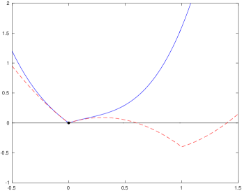
Figure 3.1: $w(x)$ (in blue) and $T_{w,2}(0,s)=T_{f,2}(0,s)+|T_{c,2}(0,s)|$ (in red)

In the non-composite ($h=0$) case, Lemma 3.2 may be extended for unconstrained (i.e., ${\cal F}=\hbox{I\hskip-2.0ptR}^{n}$) twice-continuously differentiable $f$ since then standard second-order optimality conditions at a global minimizer $x_{*}$ of $f$ imply that $T_{f,j}(x_{*},d)$ is convex for $j=1,2$ and thus that $\phi_{f,1}^{\delta}(x_{*})=\phi_{f,2}^{\delta}(x_{*})=0$. When constraints are present (i.e., ${\cal F}\subset\hbox{I\hskip-2.0ptR}^{n}$), unfortunately this may require that we restrict $\delta$. For example, the global minimizer of $f(x)=-(x-1/3)^{2}+2/3x^{3}$ for $x\in[0,1]$ lies at $x_{*}=0$, but $T_{f,2}(x_{*},d)=-(d-1/3)^{2}$ which has its constrained global minimizer at $d=1$ with $T_{f,2}(x_{*},1)<T_{f,2}(x_{*},0)$ and we would need $\delta\leq 2/3$ to ensure that $\phi_{f,2}^{\delta}(x_{*})=0$.

4 An adaptive regularization algorithm for composite
optimization

We now consider an adaptive regularization algorithm to search for a (strong) $(\epsilon,\delta)$-approximate $q$-th-order minimizer for problem (1.1), that is a point $x_{k}\in{\cal F}$ such that

$$\phi_{w,j}^{\delta}(x_{k})\leq\epsilon_{j}\,\frac{\delta_{j}^{j}}{j!}\;\;\mbox{ for }\;\;j\in\{1,\ldots,q\},$$ (4.1)

where $\phi_{w,q}^{\delta}(x)$ is defined in (3.11). At each iteration, the algorithm seeks an approximate minimizer of the (possibly non-smooth) regularized model

$$m_{k}(s)=T_{f,p}(x_{k},s)+h\big{(}T_{c,p}(x_{k},s)\big{)}+\frac{\sigma_{k}}{(p+1)!}\|s\|^{p+1}=T_{w,p}(x_{k},s)+\frac{\sigma_{k}}{(p+1)!}\|s\|^{p+1}$$ (4.2)

and this process is allowed to terminate whenever

$$m_{k}(s)\leq m_{k}(0)$$ (4.3)

and, for each $j\in\{1,\ldots,q\}$,

$$\phi_{m_{k},j}^{\delta_{s,j}}(s)\leq\theta\epsilon_{j}\,\frac{\delta_{s,j}^{j}}{j!}.$$ (4.4)

Obviously, the inclusion of $h$ in the definition of the model (4.2) implicitly assumes that, as is common, the cost of evaluation $h$ is small compared with that of evaluating $f$ or $c$. It also implies that computing $\phi_{w,j}^{\delta_{j}}(x)$ and $\phi_{m_{k},j}^{\delta_{s,j}}(s)$ is potentially more complicated than in the non-composite case, although it does not impact the evaluation complexity of the algorithm because the model’s approximate minimization does not involve evaluating $f$, $c$ or any of their derivatives.

The rest of the algorithm, that we shall refer to as AR$qp$C, follows the standard pattern of adaptive regularization algorithms, and is stated 4.

Algorithm 4.1: AR$qp$C, to find an $(\epsilon,\delta)$-approximate $q$-th-order minimizer
                          of the composite function $w$ in (1.1)
Step 0: Initialization. An initial point $x_{0}$ and an initial regularization parameter $\sigma_{0}>0$ are given, as well as an accuracy level $\epsilon\in(0,1)^{q}$. The constants $\delta_{0}$, $\theta$, $\eta_{1}$, $\eta_{2}$, $\gamma_{1}$, $\gamma_{2}$, $\gamma_{3}$ and $\sigma_{\min}$ are also given and satisfy $$\begin{array}[]{c}\theta>0,\;\;\delta_{0}\in(0,1],\;\;\sigma_{\min}\in(0,\sigma_{0}],\;\;0<\eta_{1}\leq\eta_{2}<1\\ \;\;\mbox{and}\;\;0<\gamma_{1}<1<\gamma_{2}<\gamma_{3}.\end{array}$$ (4.5) Compute $w(x_{0})$ and set $k=0$. Step 1: Test for termination. Evaluate $\{\nabla^{i}_{x}f(x_{k})\}_{i=1}^{q}$ and $\{\nabla^{i}_{x}c(x_{k})\}_{i=1}^{q}$. If (4.1) holds with $\delta=\delta_{k}$, terminate with the approximate solution $x_{\epsilon}=x_{k}$. Otherwise compute $\{\nabla^{i}_{x}f(x_{k})\}_{i=q+1}^{p}$ and $\{\nabla^{i}_{x}c(x_{k})\}_{i=q+1}^{p}$. Step 2: Step calculation. Attempt to compute an approximate minimizer $s_{k}$ of model $m_{k}(s)$ given in (4.2) such that $x_{k}+s\in{\cal F}$ and an optimality radius $\delta_{s}\in(0,1]^{q}$ such that (4.3) holds and (4.4) holds for $j\in\{1,\ldots,q\}$. If no such step exist, terminate with the approximate solution $x_{\epsilon}=x_{k}$. Step 3: Acceptance of the trial point. Compute $w(x_{k}+s_{k})$ and define $$\rho_{k}=\frac{w(x_{k})-w(x_{k}+s_{k})}{w(x_{k})-T_{w,p}(x_{k},s)}.$$ (4.6) If $\rho_{k}\geq\eta_{1}$, then define $x_{k+1}=x_{k}+s_{k}$ and $\delta_{k+1}=\delta_{s}$; otherwise define $x_{k+1}=x_{k}$ and $\delta_{k+1}=\delta_{k}$. Step 4: Regularization parameter update. Set $$\sigma_{k+1}\in\left\{\begin{array}[]{ll}{}[\max(\sigma_{\min},\gamma_{1}\sigma_{k}),\sigma_{k}]&\;\;\mbox{if}\;\;\rho_{k}\geq\eta_{2},\\ {}[\sigma_{k},\gamma_{2}\sigma_{k}]&\;\;\mbox{if}\;\;\rho_{k}\in[\eta_{1},\eta_{2}),\\ {}[\gamma_{2}\sigma_{k},\gamma_{3}\sigma_{k}]&\;\;\mbox{if}\;\;\rho_{k}<\eta_{1}.\end{array}\right.$$ (4.7) Increment $k$ by one and go to Step 1 if $\rho_{k}\geq\eta_{1}$, or to Step 2 otherwise.

As expected, the AR$qp$C algorithm shows obvious similarities with that discussed in [10], but differs from it in significant ways. Beyond the fact that it now handles composite objective functions, the main one being that the termination criterion in Step 1 now tests for strong approximate minimizers, rather than weak ones.

As is standard for adaptive regularization algorithms, we say that an iteration is successful when $\rho_{k}\geq\eta_{1}$ (and $x_{k+1}=x_{k}+s_{k}$) and that it is unsuccessful otherwise. We denote by ${\cal S}_{k}$ the index set of all successful iterations from 0 to $k$, that is

$${\cal S}_{k}=\{j\in\{0,\ldots,k\}\mid\rho_{j}\geq\eta_{1}\},$$

and then obtain a well-known result ensuring that successful iterations up to iteration $k$ do not amount to a vanishingly small proportion of these iterations.

Lemma 4.1

The mechanism of the AR$qp$C algorithm guarantees that, if $$\sigma_{k}\leq\sigma_{\max},$$ (4.8) for some $\sigma_{\max}>0$, then $$k+1\leq|{\cal S}_{k}|\left(1+\frac{|\log\gamma_{1}|}{\log\gamma_{2}}\right)+\frac{1}{\log\gamma_{2}}\log\left(\frac{\sigma_{\max}}{\sigma_{0}}\right).$$ (4.9)

• Proof.   See [3, Theorem 2.4]. $\Box$

We also have the following identity for the norm of the successive derivatives of the regularization term.

Lemma 4.2

Let $s$ be a vector of $\hbox{I\hskip-2.0ptR}^{n}$. Then $$\|\,\nabla_{s}^{j}\big{(}\|s\|^{p+1}\big{)}\,\|=\frac{(p+1)!}{(p-j+1)!}\|s\|^{p-j+1}\;\;\mbox{for}\;\;j\in\{0,\ldots,p+1\}.$$ (4.10)

• Proof.   See [10, Lemma 2.4] with $\beta=1$. $\Box$

As the conditions for accepting a pair $(s_{k},\delta_{s})$ in Step 2 are stronger than previously considered (in particular, they are stronger than those discussed in [10]), we must ensure that such acceptable pairs exist. We start by recalling a result discussed in [10] for the non-composite case.

Lemma 4.3

Suppose that $${\cal F}\;\;\mbox{is convex and }\;\;\left\{\begin{array}[]{lllll}\mbox{either}&h=0&\mbox{and}&q\in\{1,2\},\\ \mbox{or}&h\;\;\mbox{is convex}&\mbox{and}&q=1.\\ \end{array}\right.$$ (4.11) Suppose in addition that $s_{k}^{*}\neq 0$ is a global minimizer of $m_{k}(s)$ for $x_{k}+s\in{\cal F}$. Then there exist a feasible neighbourhood of $s_{k}^{*}$ such that (4.3) and (4.4) hold for any $s_{k}$ in this neighbourhood with $\delta_{s}=1$.

• Proof.    We consider the unconstrained non-composite case first. Our assumption that $s_{k}^{*}\neq 0$ implies that $m_{k}$ is $p$ times continuously differentiable at $s_{k}^{*}$. Suppose that $j=1$ ($j=2$). Then the $j$-th order Taylor expansion of the model at $s_{k}^{*}$ is a linear (positive semidefinite quadratic) polynomial, which is a convex function. As a consequence $\phi_{m_{k},j}^{\delta}(s_{k}^{*})=0$ for all $\delta_{s,j}>0$. The desired conclusion then follows by continuity of $\phi_{m_{k},j}^{\delta}(s)$ as a function of $s$.

  Consider the unconstrained composite case with convex $h$ next. Since $q=1$, the minimization subproblem remains convex, allowing us to conclude.

  Adding convex constraints does not alter the convexity of the subproblem either, and the result thus extends to convexly constrained versions of the cases considered above. $\Box$

Alas, the example given at the end of Section 3 implies that $\delta_{s}$ may have to be chosen smaller than one for $q=2$ and when $h$ is nonzero, even if it is convex. Fortunately, the existence of a step is still guaranteed in general, even without assuming convexity of $h$. To state our result, we first define $\xi$ to be an arbitrary constant in $(0,1)$ independent of $\epsilon$, which we will specify later.

Lemma 4.4

Let $\xi\in(0,1)$ and suppose that $s_{k}^{*}$ is a global minimizer of $m_{k}(s)$ for $x_{k}+s\in{\cal F}$ such that $m_{k}(s_{k}^{*})<m_{k}(0)$. Then there exists a pair $(\overline{s},\delta_{s})$ such that (4.3) and (4.4) hold. Moreover, one has that either $\|\overline{s}\|\geq\xi$ or (4.3) and (4.4) hold for $\overline{s}$ for all $\delta_{s,j}$ ($j\in\{1,\ldots,q\}$), for which $$0<\delta_{s,j}\leq\frac{\theta}{q!(6L_{w}+3\sigma_{k})}\,\epsilon_{j}.$$ (4.12)

• Proof.    We first need to show that a pair $(\overline{s},\delta_{s})$ satisfying (4.3) and (4.4) exists. Since $m_{k}(s_{k}^{*})<m_{k}(0)$, we have that $s_{k}^{*}\neq 0$. By Taylor’s theorem, we have that, for all $d$,

  $$\begin{array}[]{lcl}0&\leq&m_{k}(s_{k}^{*}+d)-m_{k}(s_{k}^{*})=\displaystyle\sum_{\ell=1}^{p}\frac{\displaystyle 1}{\displaystyle\ell!}\nabla_{s}^{\ell}T_{f,p}(x_{k},s_{k}^{*})[d]^{\ell}\\[10.76385pt] &&\hskip 14.22636pt+h\Bigg{(}\displaystyle\sum_{\ell=0}^{p}\frac{\displaystyle 1}{\displaystyle\ell!}\nabla_{s}^{\ell}T_{c,p}(x_{k},s_{k}^{*})[d]^{\ell}\Bigg{)}-h\big{(}T_{c,p}(x_{k},s_{k}^{*})\big{)}\\[10.76385pt] &&\hskip 14.22636pt+\frac{\displaystyle\sigma_{k}}{\displaystyle(p+1)!}\Bigg{[}\displaystyle\sum_{\ell=1}^{p}\frac{1}{\ell!}\nabla_{s}^{\ell}\left(\|s_{k}^{*}\|^{p+1}\right)[d]^{\ell}+\frac{1}{(p+1)!}\nabla_{s}^{p+1}\left(\|s_{k}^{*}+\tau d\|^{p+1}\right)[d]^{p+1}\Bigg{]}\end{array}$$ (4.13)

  for some $\tau\in(0,1)$. Using (4.10) in (4.13) and the subadditivity of $h$ ensured by AS.3 then yields that, for any $j\in\{1,\ldots,q\}$ and all $d$,

  $$\begin{array}[]{l}-\displaystyle\sum_{\ell=1}^{j}\frac{\displaystyle 1}{\displaystyle\ell!}\nabla_{s}^{\ell}T_{f,p}(x_{k},s_{k}^{*})[d]^{\ell}+h\big{(}T_{c,p}(x_{k},s_{k}^{*})\big{)}\\[10.76385pt] \hskip 56.9055pt-h\Bigg{(}\displaystyle\sum_{\ell=0}^{j}\frac{\displaystyle 1}{\displaystyle\ell!}\nabla_{s}^{\ell}T_{c,p}(x_{k},s_{k}^{*})[d]^{\ell}\Bigg{)}-\frac{\displaystyle\sigma_{k}}{\displaystyle(p+1)!}\displaystyle\sum_{\ell=1}^{j}\nabla_{s}^{\ell}\|s_{k}^{*}\|^{p+1}[d]^{\ell}\\[10.76385pt] \hskip 85.35826pt\leq\displaystyle\sum_{\ell=j+1}^{p}\frac{\displaystyle 1}{\displaystyle\ell!}\nabla_{s}^{\ell}T_{f,p}(x_{k},s_{k}^{*})[d]^{\ell}+h\Bigg{(}\displaystyle\sum_{\ell=j+1}^{q}\frac{\displaystyle 1}{\displaystyle\ell!}\nabla_{s}^{\ell}T_{c,p}(x_{k},s_{k}^{*})[d]^{\ell}\Bigg{)}\\[10.76385pt] \hskip 113.81102pt+\frac{\displaystyle\sigma_{k}}{\displaystyle(p+1)!}\Bigg{[}\displaystyle\sum_{\ell=j+1}^{p}\frac{1}{\ell!}\nabla_{s}^{\ell}\|s_{k}^{*}\|^{p+1}[d]^{\ell}+\|d\|^{p+1}\Bigg{]}.\end{array}$$ (4.14)

  Since $s_{k}^{*}\neq 0$, and using (3.6), we may then choose $\delta_{s,j}\in(0,1]$ such that, for every $d$ with $\|d\|\leq\delta_{s,j}$,

  $$\begin{array}[]{l}\displaystyle\sum_{\ell=j+1}^{p}\frac{\displaystyle 1}{\displaystyle\ell!}\nabla_{s}^{\ell}T_{f,p}(x_{k},s_{k}^{*})[d]^{\ell}+h\Bigg{(}\displaystyle\sum_{\ell=j+1}^{p}\frac{\displaystyle 1}{\displaystyle\ell!}\nabla_{s}^{\ell}T_{c,p}(x_{k},s_{k}^{*})[d]^{\ell}\Bigg{)}\\[10.76385pt] \hskip 85.35826pt+\frac{\displaystyle\sigma_{k}}{\displaystyle(p+1)!}\Bigg{[}\displaystyle\sum_{\ell=j+1}^{p}\frac{\displaystyle 1}{\displaystyle\ell!}\nabla_{s}^{\ell}\|s_{k}^{*}\|^{p+1}[d]^{\ell}+\|d\|^{p+1}\Bigg{]}\\[10.76385pt] \hskip 56.9055pt\leq{\scriptstyle\frac{1}{2}}\theta\epsilon_{j}\,\frac{\displaystyle\delta_{s,j}^{j}}{\displaystyle j!}.\end{array}$$ (4.15)

  As a consequence, we obtain that if $\delta_{s,j}$ is small enough to ensure (4.15), then (4.14) implies that

  $$\begin{array}[]{l}-\displaystyle\sum_{\ell=1}^{j}\frac{\displaystyle 1}{\displaystyle\ell!}\nabla_{s}^{\ell}T_{f,p}(x_{k},s_{k}^{*})[d]^{\ell}+h\big{(}T_{c,p}(x_{k},s_{k}^{*})\big{)}\\[10.76385pt] \hskip 56.9055pt-h\Bigg{(}\displaystyle\sum_{\ell=0}^{j}\frac{\displaystyle 1}{\displaystyle\ell!}\nabla_{s}^{\ell}T_{c,p}(x_{k},s_{k}^{*})[d]^{\ell}\Bigg{)}-\frac{\displaystyle\sigma_{k}}{\displaystyle(p+1)!}\displaystyle\sum_{\ell=1}^{j}\nabla_{s}^{\ell}\|s_{k}^{*}\|^{p+1}[d]^{\ell}\\[10.76385pt] \hskip 113.81102pt\leq{\scriptstyle\frac{1}{2}}\theta\epsilon_{j}\,\frac{\displaystyle\delta_{s,j}^{j}}{\displaystyle j!}.\end{array}$$ (4.16)

  The fact that, by definition,

  $$\begin{array}[]{c}\phi_{m_{k},j}^{\delta_{s,j}}(s)=\max\Big{[}0,\displaystyle\max_{\|d\|\leq\delta_{s,j}}\Big{\{}-\displaystyle\sum_{\ell=1}^{j}\frac{\displaystyle 1}{\displaystyle\ell!}\nabla_{s}^{\ell}T_{f,p}(x_{k},s)[d]^{\ell}+h\big{(}T_{c,p}(x_{k},s_{k})\big{)}\\[8.61108pt] \hskip 85.35826pt-h\Big{(}\displaystyle\sum_{\ell=0}^{j}\frac{\displaystyle 1}{\displaystyle\ell!}\nabla_{s}^{\ell}T_{c,p}(x_{k},s)[d]^{\ell}\Big{)}-\frac{\displaystyle\sigma_{k}}{\displaystyle(p+1)!}\displaystyle\sum_{\ell=1}^{j}\frac{1}{\ell!}\nabla_{s}^{\ell}\|s\|^{p+1}[d]^{\ell}\Big{\}}\Big{]},\end{array}$$ (4.17)

  continuity of $T_{f,p}(x_{k},s)$ and $T_{c,p}(x_{k},s)$ and their derivatives and the inequality $m_{k}(s_{k}^{*})<m_{k}(0)$ then ensure the existence of a feasible neighbourhood of $s_{k}^{*}\neq 0$ in which $\overline{s}$ can be chosen such that (4.3) and (4.4) hold for $s=\overline{s}$, concluding the first part of the proof.

  To prove the second part, assume first that $\|s_{k}^{*}\|\geq 1$. We may then restrict the neighbourhood of $s_{k}^{*}$ in which $\overline{s}$ can be chosen enough to ensure that $\|\overline{s}\|\geq\xi$. Assume therefore that $\|s_{k}^{*}\|\leq 1$. Remembering that, by definition and the triangle inequality,

  $$\|\nabla_{s}^{\ell}T_{f,p}(x_{k},s_{k}^{*})\|\leq\displaystyle\sum_{j=\ell}^{p}\frac{\displaystyle 1}{\displaystyle(j-\ell)!}\|\nabla_{x}^{j}f(x_{k})\|\,\|s_{k}^{*}\|^{j-\ell},$$

  $$\|\nabla_{s}^{\ell}T_{c,p}(x_{k},s_{k}^{*})\|\leq\displaystyle\sum_{j=\ell}^{p}\frac{\displaystyle 1}{\displaystyle(j-\ell)!}\|\nabla_{x}^{j}c(x_{k})\|\,\|s_{k}^{*}\|^{j-\ell},$$

  for $\ell\in\{q+1,\ldots,p\}$, and thus, using (3.6), (3.5) and (4.10), we deduce that

  $$\begin{array}[]{l}\displaystyle\sum_{\ell=j+1}^{p}\frac{\displaystyle 1}{\displaystyle\ell!}\nabla_{s}^{\ell}T_{f,p}(x_{k},s_{k}^{*})[d]^{\ell}+h\Bigg{(}\displaystyle\sum_{\ell=j+1}^{p}\frac{\displaystyle 1}{\displaystyle\ell!}\nabla_{s}^{\ell}T_{c,p}(x_{k},s_{k}^{*})[d]^{\ell}\Bigg{)}+\frac{\displaystyle\sigma_{k}}{\displaystyle(p+1)!}\Bigg{[}\displaystyle\sum_{\ell=j+1}^{p}\nabla_{s}^{\ell}\|s_{k}^{*}\|^{p+1}[d]^{\ell}\Bigg{]}\\[12.91663pt] \hskip 56.9055pt\leq\displaystyle\sum_{\ell=j+1}^{p}\frac{\displaystyle 1}{\displaystyle\ell!}\nabla_{s}^{\ell}T_{f,p}(x_{k},s_{k}^{*})[d]^{\ell}+L_{h,0}\Bigg{\|}\displaystyle\sum_{\ell=j+1}^{p}\frac{\displaystyle 1}{\displaystyle\ell!}\nabla_{s}^{\ell}T_{c,p}(x_{k},s_{k}^{*})[d]^{\ell}\Bigg{\|}\\[12.91663pt] \hskip 128.0374pt+\frac{\displaystyle\sigma_{k}}{\displaystyle(p+1)!}\Bigg{[}\displaystyle\sum_{\ell=j+1}^{p}\nabla_{s}^{\ell}\|s_{k}^{*}\|^{p+1}[d]^{\ell}\Bigg{]}\\[12.91663pt] \hskip 56.9055pt\leq\displaystyle\sum_{\ell=j+1}^{p}\frac{\displaystyle\|d\|^{\ell}}{\displaystyle\ell!}\Bigg{[}\displaystyle\sum_{i=\ell}^{p}\frac{\displaystyle\|s_{k}^{*}\|^{i-\ell}}{\displaystyle(i-\ell)!}\Big{(}\|\nabla_{x}^{i}f(x_{k})\|+L_{h,0}\|\nabla_{x}^{i}c(x_{k})\|\Big{)}\\[12.91663pt] \hskip 128.0374pt+\frac{\displaystyle\sigma_{k}\|s_{k}^{*}\|^{p-\ell+1}}{\displaystyle(p-\ell+1)!}\Bigg{]}\\[12.91663pt] \hskip 56.9055pt\leq\displaystyle\sum_{\ell=j+1}^{p}\frac{\displaystyle\|d\|^{\ell}}{\displaystyle\ell!}\Bigg{[}L_{w}\,\displaystyle\sum_{i=\ell}^{p}\frac{\displaystyle\|s_{k}^{*}\|^{i-\ell}}{\displaystyle(i-\ell)!}+\frac{\displaystyle\sigma_{k}\|s_{k}^{*}\|^{p-\ell+1}}{\displaystyle(p-\ell+1)!}\Bigg{]},\end{array}$$

  where $L_{w}$ is defined in (3.7). We therefore obtain from (4.15) that any pair $(s_{k}^{*},\delta_{s,j})$ satisfies (4.16) for $\|d\|\leq\delta_{s,j}$ if

  $$\sum_{\ell=j+1}^{p}\frac{\displaystyle\delta_{s,j}^{\ell}}{\displaystyle\ell!}\left[L_{w}\displaystyle\sum_{i=\ell}^{p}\frac{\displaystyle 1}{\displaystyle(i-\ell)!}\|s_{k}^{*}\|^{i-\ell}+\frac{\displaystyle\sigma_{k}\|s_{k}^{*}\|^{p-\ell+1}}{\displaystyle(p-\ell+1)!}\right]+\sigma_{k}\frac{\displaystyle\delta_{s,j}^{p+1}}{\displaystyle(p+1)!}\leq{\scriptstyle\frac{1}{2}}\theta\epsilon_{j}\,\frac{\displaystyle\delta_{s,j}^{j}}{\displaystyle j!}.$$ (4.18)

  which, because $\|s_{k}^{*}\|\leq 1$, is in turn ensured by the inequality

  $$\sum_{\ell=j+1}^{p}\frac{\delta_{s,j}^{\ell}}{\ell!}\left[L_{w}\,\sum_{i=\ell}^{p}\frac{1}{(j-\ell)!}+\sigma_{k}\right]+\sigma_{k}\frac{\displaystyle\delta_{s,j}^{p+1}}{\displaystyle(p+1)!}\leq{\scriptstyle\frac{1}{2}}\theta\epsilon_{j}\,\frac{\delta_{s,j}^{j}}{j!}.$$ (4.19)

  Observe now that, since $\delta_{s,j}\in[0,1]$, $\delta_{s,j}^{\ell}\leq\delta_{s,j}^{j+1}$ for $\ell\in\{j+1,\ldots,p\}$. Moreover, we have that,

  $$\sum_{i=\ell}^{p}\frac{1}{(i-\ell)!}\leq e<3,\;\;\;\;(\ell\in\{j+1,\ldots,p+1\}),\;\;\;\;\;\;\;\;\sum_{\ell=j+1}^{p+1}\frac{1}{\ell!}\leq e-1<2$$

  and therefore (4.19) is (safely) guaranteed by the condition

  $$j!(6L_{w}+3\sigma_{k})\,\delta_{s,j}\leq{\scriptstyle\frac{1}{2}}\theta\epsilon_{j},$$ (4.20)

  which means that the pair $(s_{k}^{*},\delta_{s})$ satisfies (4.16) for all $j\in\{1,\ldots,q\}$ whenever,

  $$\delta_{s,j}\leq\frac{{\scriptstyle\frac{1}{2}}\theta\epsilon_{j}}{q!(6L_{w}+3\sigma_{k})}\stackrel{{\scriptstyle\rm def}}{{=}}{\scriptstyle\frac{1}{2}}\delta_{\min,k}$$

  We may thus again invoke continuity of the derivatives of $m_{k}$ and (4.17) to deduce that there exists a neighbourhood of $s_{k}^{*}$ such that, for every $\overline{s}$ in this neighbourhood, $m_{k}(\overline{s})<m_{k}(0)$ and the pair $(\overline{s},\delta_{\min,k})$ satisfies

  $$\phi_{m_{k},j}^{\delta_{\min,k}}(\overline{s})\leq\theta\epsilon_{j}\,\frac{\delta_{\min,k}^{j}}{j!},$$

  yielding the desired conclusion. $\Box$

This lemma indicates that either the norm of the step is large, or the range of acceptable $\delta_{s,j}$ is not too small in that any positive value at most equal to (4.12) can be chosen. Thus any value larger than a fixed fraction of (4.12) is also acceptable. We therefore assume, without loss of generality, that, if some constant $\sigma_{\max}$ is given such that $\sigma_{k}\leq\sigma_{\max}$ for all $k$, then the AR$qp$ algorithm ensures that

$$\delta_{s,j}\geq\kappa_{\delta,\min}\,\epsilon_{j}\;\;\mbox{with}\;\;\kappa_{\delta,\min}\stackrel{{\scriptstyle\rm def}}{{=}}\frac{\theta}{2q!(6L_{w}+3\sigma_{\max})}\in(0,{\scriptstyle\frac{1}{2}})$$ (4.21)

for $j\in\{1,\ldots,q\}$ whenever $\|s_{k}\|\leq\xi$.

We also need to establish that the possibility of termination in Step 2 of the AR$qp$C algorithm is a satisfactory outcome. We first consider the special case already studied in Lemma 4.3.

Lemma 4.5

Suppose that $q=1$ and that $h$ is convex. Suppose also that the AR$qp$C algorithm does not terminate in Step 1 of iteration $k$. Then $s_{k}^{*}$, the step from $x_{k}$ to the global minimizer of $m_{k}(s)$, is nonzero.

• Proof.    By assumption, we have that $\phi_{w,1}^{\delta_{k}}(x_{k})>0$. Suppose now that $s_{k}^{*}=0$. Then, for any $\delta\in(0,1]$,

  $$0=\phi_{m_{k},1}^{\delta}(s_{k}^{*})=\phi_{m_{k},1}^{\delta}(0)=\phi_{w,1}^{\delta}(x_{k}).$$

  This is impossible and thus $s_{k}^{*}\neq 0$. $\Box$

Combining this result with Lemma 4.3 therefore shows that when $q=1$, Step 2 can always produce a pair $(s_{k},1)$ such that $s_{k}\neq 0$ and the pair satisfies (4.3) and (4.4). When the algorithm terminates in Step 2, we may still provide a sufficient optimality guarantee.

Lemma 4.6

Suppose AS.3 holds, and that the AR$qp$C algorithm terminates in Step 2 of iteration $k$ with $x_{\epsilon}=x_{k}$. Then there exists a $\delta\in(0,1]$ such that (4.1) holds for $x=x_{\epsilon}$ and $x_{\epsilon}$ is an $(\epsilon,\delta)$-approximate $q$th-order-necessary minimizer.

• Proof.    Given Lemma 4.4, if the algorithm terminates within Step 2, it must be because every (feasible) global minimizer $s_{k}^{*}$ of $m_{k}(s)$ is such that $m_{k}(s_{k}^{*})\geq m_{k}(0)$. In that case, $s_{k}^{*}=0$ is one such global minimizer and we have that, for any $j\in\{1,\ldots,q\}$ and all $d$ with $x_{k}+d\in{\cal F}$,

  $$\begin{array}[]{l}0\leq m_{k}(d)-m_{k}(0)=\displaystyle\sum_{\ell=1}^{j}\frac{\displaystyle 1}{\displaystyle\ell!}\nabla_{x}^{\ell}f(x_{k})[d]^{\ell}+\displaystyle\sum_{\ell=j+1}^{p}\frac{\displaystyle 1}{\displaystyle\ell!}\nabla_{x}^{\ell}f(x_{k})[d]^{\ell}\\[12.91663pt] \hskip 128.0374pt+h\Bigg{(}c(x_{k})+\displaystyle\sum_{\ell=1}^{j}\frac{\displaystyle 1}{\displaystyle\ell!}\nabla_{x}^{\ell}c(x_{k})[d]^{\ell}+\displaystyle\sum_{\ell=j+1}^{p}\frac{\displaystyle 1}{\displaystyle\ell!}\nabla_{x}^{\ell}c(x_{k})[d]^{\ell}\Bigg{)}\\[12.91663pt] \hskip 128.0374pt+\frac{\displaystyle\sigma_{k}}{\displaystyle(p+1)!}\|d\|^{p+1}-h\big{(}c(x_{k})\big{)}\\[12.91663pt] \hskip 96.73936pt\leq\displaystyle\sum_{\ell=1}^{j}\frac{\displaystyle 1}{\displaystyle\ell!}\nabla_{x}^{\ell}f(x_{k})[d]^{\ell}+\displaystyle\sum_{\ell=j+1}^{p}\frac{\displaystyle 1}{\displaystyle\ell!}\nabla_{x}^{\ell}f(x_{k})[d]^{\ell}\\[12.91663pt] \hskip 128.0374pt+h\Bigg{(}\displaystyle\sum_{\ell=1}^{j}\frac{\displaystyle 1}{\displaystyle\ell!}\nabla_{x}^{\ell}c(x_{k})[d]^{\ell}\Bigg{)}+h\Bigg{(}\displaystyle\sum_{\ell=j+1}^{p}\frac{\displaystyle 1}{\displaystyle\ell!}\nabla_{x}^{\ell}c(x_{k})[d]^{\ell}\Bigg{)}\\[12.91663pt] \hskip 128.0374pt+\frac{\displaystyle\sigma_{k}}{\displaystyle(p+1)!}\|d\|^{p+1}\\[12.91663pt] \end{array}$$

  where we used the subadditivity of $h$ (ensured by AS.3) to derive the last inequality. Hence

  $$\begin{array}[]{l}-\displaystyle\sum_{\ell=1}^{j}\frac{\displaystyle 1}{\displaystyle\ell!}\nabla_{x}^{\ell}f(x_{k})[d]^{\ell}-h\Bigg{(}\displaystyle\sum_{\ell=1}^{j}\frac{\displaystyle 1}{\displaystyle\ell!}\nabla_{x}^{\ell}c(x_{k})[d]^{\ell}\Bigg{)}\\ \hskip 28.45274pt\leq\displaystyle\sum_{\ell=j+1}^{p}\frac{\displaystyle 1}{\displaystyle\ell!}\nabla_{x}^{\ell}f(x_{k})[d]^{\ell}+h\Bigg{(}\displaystyle\sum_{\ell=j+1}^{p}\frac{\displaystyle 1}{\displaystyle\ell!}\nabla_{x}^{\ell}c(x_{k})[d]^{\ell}\Bigg{)}+\frac{\displaystyle\sigma_{k}}{\displaystyle(p+1)!}\|d\|^{p+1}\\[12.91663pt] \end{array}$$

  Using (3.6), we may now choose each $\delta_{j}\in(0,1]$ for $j\in\{1,\ldots,q\}$ small enough to ensure that the absolute value of the last right-hand side is at most $\epsilon_{j}\delta_{k,j}^{j}/j!$ for all $d$ with $\|d\|\leq\delta_{k,j}$ and $x_{k}+d\in{\cal F}$, which, in view of (3.11), implies (4.1). $\Box$

5 Evaluation complexity

To analyse the evaluation complexity of the AR$qp$C algorithm, we first derive the expected decrease in the unregularized model from (4.2).

Lemma 5.1

At every iteration $k$ of the AR$qp$C algorithm, one has that $$w(x_{k})-T_{w,p}(x_{k},s_{k})\geq\frac{\sigma_{k}}{(p+1)!}\|s_{k}\|^{p+1}.$$ (5.1)

• Proof.    Immediate from (4.2) and (3.10), the fact that $m_{k}(0)=w(x_{k})$ and (4.3). $\Box$

We next derive the existence of an upper bound on the regularization parameter for the structured composite problem. The proof of this result hinges on the fact that, once the regularization parameter $\sigma_{k}$ exceeds the relevant Lipschitz constant ($L_{w,p}$ here), there is no need to increase it any further because the model then provides an overestimation of the objective function.

Lemma 5.2

Suppose that AS.1–AS.3 hold. Then, for all $k\geq 0$, $$\sigma_{k}\leq\sigma_{\max}\stackrel{{\scriptstyle\rm def}}{{=}}\max\left[\sigma_{0},\frac{\gamma_{3}L_{w,p}}{1-\eta_{2}}\right].$$ (5.2) where $L_{w,p}=L_{f,p}+L_{h,0}L_{c,p}$.

• Proof.    Successively using (4.6), Theorem 3.1 applied to $f$ and $c$ and (5.1), we deduce that, at iteration $k$,

  $$\begin{array}[]{lcl}|\rho_{k}-1|&=&\left|\frac{\displaystyle w(x_{k})-w(x_{k}+s_{k})}{\displaystyle w(x_{k})-T_{w,p}(x_{k},s)}-1\right|\\[12.91663pt] &=&\left|\frac{\displaystyle f(x_{k}+s_{k})+h\big{(}c(x_{k}+s_{k})\big{)}-T_{f,p}(x_{k},s)-h\big{(}T_{c,p}(x_{k},s)\big{)}}{\displaystyle w(x_{k})-T_{w,p}(x_{k},s)}\right|\\[12.91663pt] &\leq&\left|\frac{\displaystyle\frac{L_{f,p}\|s_{k}\|^{p+1}}{(p+1)!}+L_{h,0}\|c(x_{k}+s_{k})-T_{c,p}(x_{k},s)\|}{\displaystyle w(x_{k})-T_{w,p}(x_{k},s)}\right|\\[21.52771pt] &\leq&\left|\frac{\displaystyle\frac{L_{f,p}+L_{h,0}L_{c,p}}{(p+1)!}\|s_{k}\|^{p+1}}{\displaystyle\frac{\sigma_{k}}{(p+1)!}\|s_{k}\|^{p+1}}\right|\\[21.52771pt] &\leq&\left|\frac{\displaystyle L_{f,p}+L_{h,0}L_{c,p}}{\displaystyle\sigma_{k}}\right|.\end{array}$$

  Thus, if $\sigma_{k}\geq L_{w,p}/(1-\eta_{2})$, then iteration $k$ is successful, $x_{k+1}=x_{k}$ and (4.7) implies that $\sigma_{k+1}\leq\sigma_{k}$. The conclusion then follows from the mechanism of (4.7). $\Box$

We now establish an important inequality derived from our smoothness assumptions.

Lemma 5.3

Suppose that AS.1–AS.3 hold. Suppose also that iteration $k$ is successful and that the ARqpC algorithm does not terminate at iteration $k+1$. Then there exists a $j\in\{1,\ldots,q\}$ such that $$(1-\theta)\,\epsilon\,\frac{\displaystyle\delta_{k+1,j}^{j}}{\displaystyle j!}\leq(L_{w,p}+\sigma_{\max})\displaystyle\sum_{\ell=1}^{j}\frac{\displaystyle\delta_{k+1,j}^{\ell}}{\displaystyle\ell!}\|s_{k}\|^{p-\ell+1}+2\frac{\displaystyle L_{h,0}L_{c,p}}{\displaystyle(p+1)!}\|s_{k}\|^{p+1}.$$ (5.3)

• Proof.   If the algorithm does not terminate at iteration $k+1$, there must exist a $j\in\{1,\ldots,q\}$ such that (4.1) fails at order $j$ at iteration $k+1$. Consider such a $j$ and let $d$ be the argument of the minimization in the definition of $\phi_{w,j}^{\delta_{k+1,j}}(x_{k+1})$. Then $x_{k}+d\in{\cal F}$ and $\|d\|\leq\delta_{k+1,j}\leq 1$. The definition of $\phi_{w,j}^{\delta_{k+1,j}}(x_{k+1})$ in (3.11) then gives that

  $$\begin{array}[]{l}\epsilon\frac{\displaystyle\delta_{k+1,j}^{j}}{\displaystyle j!}<\phi_{w,j}^{\delta_{k+1,j}}(x_{k+1})\\[12.91663pt] \hskip 28.45274pt=-\displaystyle\sum_{\ell=1}^{j}\frac{1}{\ell!}\nabla_{x}^{\ell}f(x_{k+1})[d]^{\ell}+h\big{(}c(x_{k+1})\big{)}-h\Bigg{(}\displaystyle\sum_{\ell=0}^{j}\frac{1}{\ell!}\nabla_{x}^{\ell}c(x_{k+1})[d]^{\ell}\Bigg{)}\\[12.91663pt] \hskip 28.45274pt=-\displaystyle\sum_{\ell=1}^{j}\frac{1}{\ell!}\nabla_{x}^{\ell}f(x_{k+1})[d]^{\ell}+\displaystyle\sum_{\ell=1}^{j}\frac{\displaystyle 1}{\displaystyle\ell!}\nabla^{\ell}_{s}T_{f,p}(x_{k},s_{k})[d]^{\ell}\\[12.91663pt] \hskip 56.9055pt+h\big{(}c(x_{k+1})\big{)}-h\big{(}T_{c,p}(x_{k},s_{k})\big{)}\\[12.91663pt] \hskip 56.9055pt-h\Bigg{(}\displaystyle\sum_{\ell=0}^{j}\frac{1}{\ell!}\nabla_{x}^{\ell}c(x_{k+1})[d]^{\ell}\Bigg{)}+h\Bigg{(}\displaystyle\sum_{\ell=0}^{j}\frac{\displaystyle 1}{\displaystyle\ell!}\nabla^{\ell}_{s}T_{c,p}(x_{k},s_{k})[d]^{\ell}\Bigg{)}\\[12.91663pt] \hskip 56.9055pt-\displaystyle\sum_{\ell=1}^{j}\frac{\displaystyle 1}{\displaystyle\ell!}\nabla^{\ell}_{s}T_{f,p}(x_{k},s_{k})[d]^{\ell}+h\big{(}T_{c,p}(x_{k},s_{k})\big{)}\\[12.91663pt] \hskip 56.9055pt-h\Bigg{(}\displaystyle\sum_{\ell=0}^{j}\frac{\displaystyle 1}{\displaystyle\ell!}\nabla^{\ell}_{s}T_{c,p}(x_{k},s_{k})[d]^{\ell}\Bigg{)}-\displaystyle\sum_{\ell=1}^{j}\frac{\displaystyle\sigma_{k}\|s_{k}\|^{p-\ell+1}[d]^{\ell}}{\displaystyle\ell!(p-\ell+1)!}\\[12.91663pt] \hskip 56.9055pt+\displaystyle\sum_{\ell=1}^{j}\frac{\displaystyle\sigma_{k}\|s_{k}\|^{p-\ell+1}[d]^{\ell}}{\displaystyle\ell!(p-\ell+1)!}.\end{array}$$ (5.4)

  Now, using Theorem 3.1 for $r=f$,

  $$\begin{array}[]{l}-\displaystyle\sum_{\ell=1}^{j}\frac{1}{\ell!}\nabla_{x}^{\ell}f(x_{k+1})[d]^{\ell}+\displaystyle\sum_{\ell=1}^{j}\frac{\displaystyle 1}{\displaystyle\ell!}\nabla^{\ell}_{s}T_{f,p}(x_{k},s_{k})[d]^{\ell}\\[8.61108pt] \hskip 56.9055pt\leq\displaystyle\sum_{\ell=1}^{j}\frac{\displaystyle\delta_{k+1,j}^{\ell}}{\displaystyle\ell!}\big{\|}\nabla_{x}^{\ell}f(x_{k+1})-\nabla^{\ell}_{s}T_{f,p}(x_{k},s_{k})\big{\|}\\[8.61108pt] \hskip 56.9055pt\leq L_{f,p}\displaystyle\sum_{\ell=1}^{j}\frac{\displaystyle\delta_{k+1,j}^{\ell}}{\displaystyle\ell!(p-\ell+1)!}\|s_{k}\|^{p-\ell+1}.\\[8.61108pt] \end{array}$$ (5.5)

  In the same spirit, also using AS.3 and applying Theorem 3.1 to $c$, we obtain that

  $$\begin{array}[]{l}-h\Bigg{(}\displaystyle\sum_{\ell=0}^{j}\frac{1}{\ell!}\nabla_{x}^{\ell}c(x_{k+1})[d]^{\ell}\Bigg{)}+h\Bigg{(}\displaystyle\sum_{\ell=0}^{j}\frac{\displaystyle 1}{\displaystyle\ell!}\nabla^{\ell}_{s}T_{c,p}(x_{k},s_{k})[d]^{\ell}\Bigg{)}\\[8.61108pt] \hskip 56.9055pt\leq L_{h,0}\Bigg{\|}\displaystyle\sum_{\ell=0}^{j}\frac{\displaystyle 1}{\displaystyle\ell!}\big{[}\nabla_{x}^{\ell}c(x_{k+1})-\nabla^{\ell}_{s}T_{c,p}(x_{k},s_{k})\big{]}[d]^{\ell}\Bigg{\|}\\[8.61108pt] \hskip 56.9055pt\leq L_{h,0}\displaystyle\sum_{\ell=0}^{j}\frac{\displaystyle\delta_{k+1,j}^{\ell}}{\displaystyle\ell!}\big{\|}\nabla_{x}^{\ell}c(x_{k+1})-\nabla^{\ell}_{s}T_{c,p}(x_{k},s_{k})\big{\|}\\[8.61108pt] \hskip 56.9055pt\leq L_{h,0}L_{c,p}\displaystyle\sum_{\ell=0}^{j}\frac{\displaystyle\delta_{k+1,j}^{\ell}}{\displaystyle\ell!(p-\ell+1)!}\|s_{k}\|^{p-\ell+1}\\[8.61108pt] \end{array}$$ (5.6)

  and that

  $$h\big{(}c(x_{k+1})\big{)}-h\big{(}T_{c,p}(x_{k},s_{k})\big{)}\leq L_{h,0}\|c(x_{k+1})-T_{c,p}(x_{k},s_{k})\|\leq\frac{\displaystyle L_{h,0}L_{c,p}}{\displaystyle(p+1)!}\|s_{k}\|^{p+1}.$$ (5.7)

  Because of Lemma 5.2 we also have that

  $$\sum_{\ell=1}^{j}\frac{\displaystyle\sigma_{k}\|s_{k}\|^{p-\ell+1}\delta_{k+1,j}^{\ell}}{\displaystyle\ell!(p-\ell+1)!}\leq\sigma_{\max}\displaystyle\sum_{\ell=1}^{j}\frac{\displaystyle\|s_{k}\|^{p-\ell+1}\delta_{k+1,j}^{\ell}}{\displaystyle\ell!(p-\ell+1)!}.$$ (5.8)

  Moreover, in view of (4.2) and (4.4),

  $$\begin{array}[]{l}-\displaystyle\sum_{\ell=1}^{j}\frac{\displaystyle 1}{\displaystyle\ell!}\nabla^{\ell}_{s}T_{f,p}(x_{k},s_{k})[d]^{\ell}+h\big{(}T_{c,p}(x_{k},s_{k})\big{)}-h\Bigg{(}\displaystyle\sum_{\ell=0}^{j}\frac{\displaystyle 1}{\displaystyle\ell!}\nabla^{\ell}_{s}T_{c,p}(x_{k},s_{k})[d]^{\ell}\Bigg{)}\\[8.61108pt] \hskip 85.35826pt-\displaystyle\sum_{\ell=1}^{j}\frac{\displaystyle\sigma_{k}}{\displaystyle\ell!(p-\ell+1)!}\|s_{k}\|^{p-\ell+1}\delta_{k+1,j}^{\ell}\\[8.61108pt] \hskip 42.67912pt\leq\phi_{m_{k},j}^{\delta_{s,j}}(s_{k})\\[8.61108pt] \hskip 42.67912pt=\theta\epsilon\,\frac{\displaystyle\delta_{k+1,j}^{j}}{\displaystyle j!},\end{array}$$ (5.9)

  where the last equality is derived using the fact that $\delta_{s,j}=\delta_{k+1,j}$ if iteration $k$ is successful. We may now substitute (5.5)–(5.9) into (5.4) and use the inequality $(p-\ell+1)!\geq 1$ to obtain (5.3). $\Box$

Lemma 5.4

Suppose that AS.1–AS.3 hold, that iteration $k$ is successful and that the AR$qp$C algorithm does not terminate at iteration $k+1$. Suppose also that the algorithm ensures, for each $k$, that either $\delta_{k+1,j}=1$ for $j\in\{1,\ldots,q\}$ if (4.11) holds (as allowed by Lemma 4.3), or that (4.21) holds (as allowed by Lemma 4.4) otherwise. Then there exists a $j\in\{1,\ldots,q\}$ such that $$\|s_{k}\|\geq\left\{\begin{array}[]{ll}\left(\frac{\displaystyle 1-\theta}{\displaystyle 3j!(L_{w,p}+\sigma_{\max})}\right)^{\frac{1}{p-j+1}}\,\epsilon_{j}^{\frac{1}{p-j+1}}&\;\;\mbox{if (\ref{good-cases}) holds,}\\[15.0694pt] \left(\frac{\displaystyle(1-\theta)\kappa_{\delta,\min}^{j-1}}{\displaystyle 3j!(L_{w,p}+\sigma_{\max})}\right)^{\frac{1}{p}}\,\epsilon_{j}^{\frac{j}{p}}&\;\;\mbox{if (\ref{good-cases}) fails but}\;\;h=0,\\[15.0694pt] \left(\frac{\displaystyle(1-\theta)\kappa_{\delta,\min}^{j}}{\displaystyle 3j!(L_{w,p}+\sigma_{\max})}\right)^{\frac{1}{p+1}}\,\epsilon_{j}^{\frac{j+1}{p+1}}&\;\;\mbox{if (\ref{good-cases}) fails and}\;\;h\neq 0,\end{array}\right.$$ (5.10) where $\kappa_{\delta,\min}$ is defined in (4.21).

• Proof.   We now use our freedom to choose $\xi\in(0,1)$. Let

  $$\xi\stackrel{{\scriptstyle\rm def}}{{=}}\left(\frac{\displaystyle 1-\theta}{\displaystyle 3q!(L_{w,p}+\sigma_{\max})}\right)^{\frac{1}{p-q+1}}=\min_{j\in\{1,\ldots,q\}}\left(\frac{\displaystyle 1-\theta}{\displaystyle 3j!(L_{w,p}+\sigma_{\max})}\right)^{\frac{1}{p-j+1}}\in(0,1).$$

  If $\|s_{k}\|\geq\xi$, (5.10) clearly holds since $\epsilon\leq 1$ and $\kappa_{\delta,\min}<1$. We therefore assume that $\|s_{k}\|<\xi$. Because the algorithm has not terminated, Lemma 5.3 ensures that (5.3) holds for some $j\in\{1,\ldots,q\}$. It is easy to verify that this inequality is equivalent to

  $$\alpha\,\epsilon\,\delta_{k+1,j}^{j}\leq\|s_{k}\|^{p+1}\chi_{j}\left(\frac{\delta_{k+1,j}}{\|s_{k}\|}\right)+\beta\|s_{k}\|^{p+1}$$ (5.11)

  where the function $\chi_{j}$ is defined in (2.5) and where we have set

  $$\alpha=\frac{1-\theta}{j!(L_{w,p}+\sigma_{\max})}\;\;\mbox{ and }\;\;\beta=\frac{2}{(p+1)!}\,\frac{L_{h,0}L_{c,p}}{L_{w,p}+\sigma_{\max}}\in[0,1),$$

  the last inclusion resulting from the definition of $L_{w,p}$ in Lemma 5.2. In particular, since $\chi_{j}(t)\leq 2t^{j}$ for $t\geq 1$ and $\beta<1$, we have that, when $\|s_{k}\|\leq\delta_{k+1,j}$,

  $$\alpha\,\epsilon\leq 2\|s_{k}\|^{p+1}\left(\frac{1}{\|s_{k}\|}\right)^{j}+\left(\frac{\|s_{k}\|}{\delta_{k+1,j}}\right)^{j}\|s_{k}\|^{p-j+1}\leq 3\|s_{k}\|^{p-j+1}.$$ (5.12)

  Suppose first that (4.11) hold. Then, from our assumptions, $\delta_{k+1,j}=1$ and $\|s_{k}\|\leq\xi<1=\delta_{k+1,j}$. Thus (5.12) yields the first case of (5.10). Suppose now that (4.11) fails. Then our assumptions imply that (4.21) holds. If $\|s_{k}\|\leq\delta_{k+1,j}$, we may again deduce from (5.12) that the first case of (5.10) holds, which implies, because $\kappa_{\delta,\min}<1$, that the second and third cases also hold. Consider therefore the case where $\|s_{k}\|>\delta_{k+1,j}$ and suppose first that $\beta=0$. Then (5.11) and the fact that $\chi_{j}(t)<2t$ for $t\in[0,1]$ give that

  $$\alpha\,\epsilon\,\delta_{k+1,j}^{j}\leq 2\|s_{k}\|^{p+1}\left(\frac{\delta_{k+1,j}}{\|s_{k}\|}\right),$$

  which, with (4.21) implies the second case of (5.10). Finally, if $\beta>0$, (5.11), the bound $\beta\leq 1$ and $\chi_{j}(t)<2$ for $t\in[0,1]$ ensure that

  $$\alpha\epsilon\delta_{k+1,j}^{j}\leq 2\|s_{k}\|^{p+1}+\|s_{k}\|^{p+1}$$

  the third case of (5.10) then follows from (4.21). $\Box$

Observe that the proof of this lemma ensures the better lower bound given by the first case of (5.10) whenever $\|s_{k}\|\leq\delta_{k+1,j}$. Unfortunately, there is no guarantee that this inequality holds when (4.11) fails.

We may then derive our final evaluation complexity results. To make them clearer, we provide separate statements for the standard non-composite case and for the general composite one.

  

Theorem 5.5

(Non-composite case)
    Suppose that AS.1 and AS.4 hold and that $h=0$. Suppose also that the algorithm ensures, for each $k$, that either $\delta_{k+1,j}=1$ for $j\in\{1,\ldots,q\}$ if (4.11) holds (as allowed by Lemma 4.3), or that (4.21) holds (as allowed by Lemma 4.4) otherwise. 1. Suppose that ${\cal F}$ is convex and $q\in\{1,2\}$. Then there exist positive constants $\kappa_{\sf ARqp}^{s,1}$, $\kappa^{a,1}_{\sf ARqp}$ and $\kappa^{c}_{\sf ARqp}$ such that, for any $\epsilon\in(0,1]^{q}$, the AR$qp$C algorithm requires at most $$\kappa^{a,1}_{\sf ARqp}\frac{w(x_{0})-w_{\rm low}}{\displaystyle\min_{j\in\{1,\ldots,q\}}\epsilon_{j}^{\frac{p+1}{p-j+1}}}+\kappa^{c}_{\sf ARqp}={\cal O}\left(\displaystyle\max_{j\in\{1,\ldots,q\}}\epsilon_{j}^{-\frac{p+1}{p-j+1}}\right)$$ (5.13) evaluations of $f$ and $c$, and at most $$\kappa_{\sf ARqp}^{s,1}\frac{w(x_{0})-w_{\rm low}}{\displaystyle\min_{j\in\{1,\ldots,q\}}\epsilon_{j}^{\frac{p+1}{p-j+1}}}+1={\cal O}\left(\displaystyle\max_{j\in\{1,\ldots,q\}}\epsilon_{j}^{-\frac{p+1}{p-j+1}}\right)$$ (5.14) evaluations of the derivatives of $f$ of orders one to $p$ to produce an iterate $x_{\epsilon}$ such that $\phi_{f,j}^{1}(x_{\epsilon})\leq\epsilon_{j}/j!$ for all $j\in\{1,\ldots,q\}$.  

  2. Suppose that ${\cal F}$ is nonconvex or that $q>2$. Then there exist positive constants $\kappa^{s,2}_{\sf ARqp}$, $\kappa^{a,2}_{\sf ARqp}$ and $\kappa^{c}_{\sf ARqp}$ such that, for any $\epsilon\in(0,1]^{q}$, the AR$qp$C algorithm requires at most $$\kappa^{a,2}_{\sf ARqp}\frac{w(x_{0})-w_{\rm low}}{\displaystyle\min_{j\in\{1,\ldots,q\}}\epsilon_{j}^{\frac{j(p+1)}{p}}}+\kappa^{c}_{\sf ARqp}={\cal O}\left(\displaystyle\max_{j\in\{1,\ldots,q\}}\epsilon_{j}^{-\frac{j(p+1)}{p}}\right)$$ (5.15) evaluations of $f$ and $c$, and at most $$\kappa^{s,2}_{\sf ARqp}\frac{w(x_{0})-w_{\rm low}}{\displaystyle\min_{j\in\{1,\ldots,q\}}\epsilon_{j}^{\frac{j(p+1)}{p}}}+1={\cal O}\left(\displaystyle\max_{j\in\{1,\ldots,q\}}\epsilon_{j}^{-\frac{j(p+1)}{p}}\right)$$ (5.16) evaluations of the derivatives of $f$ of orders one to $p$ to produce an iterate $x_{\epsilon}$ such that $\phi_{f,j}^{\delta_{\epsilon}}(x_{\epsilon})\leq\epsilon_{j}\,\delta_{\epsilon,j}^{j}/j!$ for some $\delta_{\epsilon}\in(0,1]^{q}$ and all $j\in\{1,\ldots,q\}$.    

  

Theorem 5.6

(Composite case)
    Suppose that AS.1–AS.4 hold. Suppose also that the algorithm ensures, for each $k$, that either $\delta_{k+1,j}=1$ for $j\in\{1,\ldots,q\}$ if (4.11) holds (as allowed by Lemma 4.3), or that (4.21) holds (as allowed by Lemma 4.4) otherwise. 1. Suppose that ${\cal F}$ is convex, $q=1$ and $h$ is convex. Then there exist positive constants $\kappa^{s,1}_{\sf ARqpC}$, $\kappa^{a,1}_{\sf ARqpC}$ and $\kappa^{c}_{\sf ARqpC}$ such that, for any $\epsilon_{1}\in(0,1]$, the AR$qp$C algorithm requires at most $$\kappa^{a,1}_{\sf ARqpC}\frac{w(x_{0})-w_{\rm low}}{\epsilon_{1}^{\frac{p+1}{p}}}+\kappa^{c,1}_{\sf ARqpC}={\cal O}\left(\epsilon_{1}^{-\frac{p+1}{p}}\right)$$ (5.17) evaluations of $f$ and $c$, and at most $$\kappa^{s,1}_{\sf ARqpC}\frac{w(x_{0})-w_{\rm low}}{\epsilon_{1}^{\frac{p+1}{p}}}+1={\cal O}\left(\epsilon^{-\frac{p+1}{p}}\right)$$ (5.18) evaluations of the derivatives of $f$ and $c$ of orders one to $p$ to produce an iterate $x_{\epsilon}$ such that $\phi_{w,j}^{1}(x_{\epsilon})\leq\epsilon_{1}$ for all $j\in\{1,\ldots,q\}$.  

  2. Suppose that ${\cal F}$ is nonconvex or that $h$ is nonconvex or that $q>1$. Then there exist positive constants $\kappa^{s,2}_{\sf ARqp}$, $\kappa^{a,2}_{\sf ARqp}$ and $\kappa^{c}_{\sf ARqp}$ such that, for any $\epsilon\in(0,1]^{q}$, the AR$qp$C algorithm requires at most $$\kappa^{a,2}_{\sf ARqpC}\frac{w(x_{0})-w_{\rm low}}{\displaystyle\min_{j\in\{1,\ldots,q\}}\epsilon_{j}^{j+1}}+\kappa^{c}_{\sf ARqpC}={\cal O}\left(\displaystyle\max_{j\in\{1,\ldots,q\}}\epsilon_{j}^{-(j+1)}\right)$$ (5.19) evaluations of $f$ and $c$, and at most $$\kappa^{s,2}_{\sf ARqpC}\frac{w(x_{0})-w_{\rm low}}{\displaystyle\min_{j\in\{1,\ldots,q\}}\epsilon_{j}^{j+1}}+1={\cal O}\left(\displaystyle\max_{j\in\{1,\ldots,q\}}\epsilon_{j}^{-(j+1)}\right)$$ (5.20) evaluations of the derivatives of $f$ and $c$ of orders one to $p$ to produce an iterate $x_{\epsilon}$ such that $\phi_{w,j}^{\delta_{\epsilon}}(x_{\epsilon})\leq\epsilon_{j}\,\delta_{\epsilon,j}^{j}/j!$ for some $\delta_{\epsilon}\in(0,1]^{q}$ and all $j\in\{1,\ldots,q\}$.    

• Proof.    We prove Theorems 5.5 and 5.6 together. At each successful iteration $k$ of the AR$qp$C algorithm before termination, we have the guaranteed decrease

  $$w(x_{k})-w(x_{k+1})\geq\eta_{1}(T_{w,p}(x_{k},0)-T_{w,p}(x_{k},s_{k}))\geq\frac{\displaystyle\eta_{1}\sigma_{\min}}{\displaystyle(p+1)!}\;\|s_{k}\|^{p+1}$$ (5.21)

  where we used (5.1) and (4.7). We now wish to substitute the bounds given by Lemma 5.4 in (5.21), and deduce that, for some $j\in\{1,\ldots,q\}$,

  $$w(x_{k})-w(x_{k+1})\geq\kappa^{-1}\epsilon_{j}^{\omega}$$ (5.22)

  where the definition of $\kappa$ and $\omega$ depends on $q$ and $h$. Specifically,

  $$\kappa\stackrel{{\scriptstyle\rm def}}{{=}}\left\{\begin{array}[]{l}\kappa^{s,1}_{\sf ARqp}=\kappa^{s,1}_{\sf ARqpC}\stackrel{{\scriptstyle\rm def}}{{=}}\left(\frac{\displaystyle 1-\theta}{\displaystyle 3j!(L_{w,p}+\sigma_{\max})}\right)^{-\frac{p+1}{p-j+1}}\\[8.61108pt] \hskip 142.26378pt\;\;\mbox{if}\;\;(q=1,\;h\;\;\mbox{and}\;\;{\cal F}\;\;\mbox{are convex), and}\\ \hskip 142.26378pt\;\;\mbox{if}\;\;(q\in\{1,2\},\;{\cal F}\;\;\mbox{is convex and}\;\;h=0),\\[8.61108pt] \kappa^{s,2}_{\sf ARqp}\stackrel{{\scriptstyle\rm def}}{{=}}\left(\frac{\displaystyle(1-\theta)\kappa_{\delta,\min}^{j-1}}{\displaystyle 3j!(L_{w,p}+\sigma_{\max})}\right)^{-\frac{p+1}{p}}\\[8.61108pt] \hskip 142.26378pt\;\;\mbox{if}\;\;h=0\;\;\mbox{and}\;\;(q>2\;\;\mbox{or}\;\;{\cal F}\;\;\mbox{is nonconvex)}\\[8.61108pt] \kappa^{s,2}_{\sf ARqpC}\stackrel{{\scriptstyle\rm def}}{{=}}\left(\frac{\displaystyle(1-\theta)\kappa_{\delta,\min}^{j}}{\displaystyle 3j!(L_{w,p}+\sigma_{\max})}\right)^{-1}\\[8.61108pt] \hskip 142.26378pt\;\;\mbox{if}\;\;h\neq 0\;\;\mbox{and}\;\;(q>1\;\;\mbox{or}\;\;{\cal F}\;\;\mbox{is nonconvex),}\end{array}\right.$$

  where $\kappa_{\delta,\min}$ is given by (4.21), and

  $$\omega\stackrel{{\scriptstyle\rm def}}{{=}}\left\{\begin{array}[]{ll}\frac{\displaystyle p+1}{\displaystyle p-q+1}&\;\;\mbox{if}\;\;(q=1,\;h\;\;\mbox{and}\;\;{\cal F}\;\;\mbox{are convex), and}\\ &\;\;\mbox{if}\;\;(q=2,\;{\cal F}\;\;\mbox{is convex and}\;\;h=0),\\[8.61108pt] \frac{\displaystyle q(p+1)}{\displaystyle p}&\;\;\mbox{if}\;\;h=0\;\;\mbox{and}\;\;(q>2\;\;\mbox{or}\;\;{\cal F}\;\;\mbox{is nonconvex)}\\[8.61108pt] q+1&\;\;\mbox{if}\;\;h\neq 0\;\;\mbox{and}\;\;(q>1\;\;\mbox{or}\;\;{\cal F}\;\;\mbox{is nonconvex).}\end{array}\right.$$

  Thus, since $\{w(x_{k})\}$ decreases monotonically,

  $$w(x_{0})-w(x_{k+1})\geq\kappa^{-1}\,\min_{j\in\{1,\ldots,q\}}\epsilon_{j}^{\omega}\,|{\cal S}_{k}|.$$

  Using AS.4, we conclude that

  $$|{\cal S}_{k}|\leq\kappa\,\frac{w(x_{0})-w_{\rm low}}{\displaystyle\min_{j\in\{1,\ldots,q\}}\epsilon_{j}^{\omega}}$$ (5.23)

  until termination, bounding the number of successful iterations. Lemma 4.1 is then invoked to compute the upper bound on the total number of iterations, yielding the constants

  $$\kappa^{a,1}_{\sf ARqp}\stackrel{{\scriptstyle\rm def}}{{=}}\kappa^{s,1}_{\sf ARqp}\left(1+\frac{|\log\gamma_{1}|}{\log\gamma_{2}}\right),\;\;\;\;\kappa^{a,2}_{\sf ARqp}\stackrel{{\scriptstyle\rm def}}{{=}}\kappa^{s,2}_{\sf ARqp}\left(1+\frac{|\log\gamma_{1}|}{\log\gamma_{2}}\right),$$

  $$\kappa^{a,1}_{\sf ARqpC}\stackrel{{\scriptstyle\rm def}}{{=}}\kappa^{s,1}_{\sf ARqpC}\left(1+\frac{|\log\gamma_{1}|}{\log\gamma_{2}}\right),\;\;\;\;\kappa^{a,2}_{\sf ARqpC}\stackrel{{\scriptstyle\rm def}}{{=}}\kappa^{s,2}_{\sf ARqpC}\left(1+\frac{|\log\gamma_{1}|}{\log\gamma_{2}}\right),$$

  and

  $$\kappa^{c}_{\sf ARqp}=\kappa^{c}_{\sf ARqpC}\stackrel{{\scriptstyle\rm def}}{{=}}\frac{1}{\log\gamma_{2}}\log\left(\frac{\sigma_{\max}}{\sigma_{0}}\right),$$

  where $\sigma_{\max}=\max\left[\sigma_{0},\frac{\displaystyle\gamma_{3}L_{w,p}}{\displaystyle 1-\eta_{2}}\right]$ (see (5.2)). The desired conclusions then follow from the fact that each iteration involves one evaluation of $f$ and each successful iteration one evaluation of its derivatives. $\Box$

For the standard non-composite case, Theorem 5.5 provides the first results on the complexity of finding strong minimizers of arbitrary orders using adaptive regularization algorithms that we are aware of. By comparison, [10] provides similar results but for the convergence to weak minimizers (see (2.5)). Unsurprisingly, the worst-case complexity bounds for weak minimizers are better than those for strong ones: the ${\cal O}\big{(}\epsilon^{-(p+1)/(p-q+1)}\big{)}$ bound which we have derived for $q\in\{1,2\}$ then extends to any order $q$. Moreover, thee full power of AS.1 is not needed for these results since it is sufficient to assume that $\nabla_{x}^{p}f(x)$ is Lipschitz continuous. It is interesting to note that the results for weak and strong approximate minimizers coincide for first and second order. The results of Theorem 5.5 may also be compared with the bound in ${\cal O}\big{(}\epsilon^{-(q+1)}\big{)}$ which was proved for trust-region methods in [9]. While these trust-region bounds do not depend on the degree of the model, those derived above for the ARqpC algorithm show that worst-case performance improves with $p$ and is always better than that of trust-region methods. It is also interesting to note that the bound obtained in Theorem 5.5 for order $q$ is identical to that which would be obtained for first-order but using $\epsilon^{q}$ instead of $\epsilon$. This reflects the observation that, at variance with weak approximate optimality, the very definition of strong approximate optimality in (2.4) requires very high accuracy on the (usually dominant) low orders terms of the Taylor series while the requirement lessens as the order increases.

An interesting feature of the algorithm discussed in [10] is that computing and testing the value of $\phi_{m_{k},j}^{\delta}(s_{k})$ is unnecessary if the length of the step is large enough. The same feature can easily be introduced into the ARqpC algorithm. Specifically, we may redefine Step 2 to accept a step as soon as (4.3) holds and

$$\|s_{k}\|\geq\left\{\begin{array}[]{ll}\varpi\displaystyle\min_{j\in\{1,\ldots,q\}}\epsilon_{j}^{\frac{1}{p-q+1}}&\;\;\mbox{if}\;\;(q=1,\;h\;\;\mbox{and}\;\;{\cal F}\;\;\mbox{are convex), and}\\ &\;\;\mbox{if}\;\;(q\in\{1,2\},\;{\cal F}\;\;\mbox{is convex and}\;\;h=0)\\ \varpi\displaystyle\min_{j\in\{1,\ldots,q\}}\epsilon_{j}^{\frac{q}{p}}&\;\;\mbox{if}\;\;h=0\;\;\mbox{and}\;\;(q>2\;\;\mbox{or}\;\;{\cal F}\;\;\mbox{is nonconvex)}\\ \varpi\displaystyle\min_{j\in\{1,\ldots,q\}}\epsilon_{j}^{\frac{q+1}{p+1}}&\;\;\mbox{if}\;\;h\neq 0\;\;\mbox{and}\;\;(q>1\;\;\mbox{or}\;\;{\cal F}\;\;\mbox{is nonconvex.)}\end{array}\right.$$

for some $\varpi\in(\theta,1]$. If these conditions fail, then one still needs to verify the requirements (4.3) and (4.4), as we have done previously. Given Lemma 5.1 and the proof of Theorems 5.5 and 5.6, it is easy to verify that this modification does not affect the conclusions of these complexity theorems, while potentially avoiding significant computations.

Existing complexity results for (possibly non-smooth) composite problems are few [6, 11, 12, 17]. Theorem 5.6 provides, to our knowledge, the first upper complexity bounds for optimality orders exceeding one, with the exception of [11] (but this paper requires strong specific assumptions on ${\cal F}$). While equivalent to those of Theorem 5.5 for the standard case when $q=1$, they are not as good and match those obtained for the trust-region methods when $q>1$. They could be made identical in order of $\epsilon_{j}$ to those of Theorem 5.5 if one is ready to assume that $L_{h,0}L_{c,p}$ is sufficiently small (for instance if $c$ is a polynomial of degree less than $p$). In this case, the constant $\beta$ in Lemmas 5.11 will of the order of $\delta_{k+1,j}/\|s_{k}\|$, leading to the better bound.

6 Sharpness

We now show that the upper bounds of Theorem 5.5 and the first part of Theorem 5.6 are sharp. Since it is sufficient for our purposes, we assume in this section that $\epsilon_{j}=\epsilon$ for all $j\in\{1,\ldots,q\}$.

We first consider a first class of problems, where the choice of $\delta_{k,j}=1$ is allowed. Since it is proved in [10] that the order in $\epsilon$ given by the Theorem 5.5 is sharp for finding weak approximate minimizers for the standard (non-composite) case, it is not surprising that this order is also sharp for the stronger concept of optimality whenever the same bound applies, that is when $q\in\{1,2\}$. However, the ARqpC algorithm slightly differs from the algorithm discussed in [10]. Not only are the termination tests for the algorithm itself and those for the step computation weaker in [10], but the algorithm there makes a provision to avoid computing $\phi_{m_{k},j}^{\delta}$ whenever the step is large enough, as discussed at the end of the last section. It is thus impossible to use the example of slow convergence provided in [10, Section 5.2] directly, but we now propose a variant that fits our present framework.

Theorem 6.1

Suppose that $h=0$ and that the choice $\delta_{k,j}=1$ is possible (and made) for all $k$ and all $j\in\{1,\ldots,q\}$. Then, for $\epsilon$ sufficiently small, the AR$qp$C algorithm applied to minimize $f$ may require $$\epsilon^{-\frac{p+1}{p-q+1}}$$ iterations and evaluations of $f$ and of its derivatives of order one up to $p$ to produce a point $x_{\epsilon}$ such that $\phi_{w,q}^{\delta_{\epsilon,j}}(x_{\epsilon})\leq\epsilon\delta_{\epsilon,j}^{j}/j!$ for some $\delta_{\epsilon}\in(0,1]^{q}$ and all $j\in\{1,\ldots,q\}$.

• Proof.    Our aim is to show that, for each choice of $p\geq 1$, there exists an objective function satisfying AS.1 and AS.4 such that obtaining a strong $(\epsilon,\delta)$-approximate $q$-th-order-necessary minimizer may require at least $\epsilon^{-(p+1)/(p-q+1)}$ evaluations of the objective function and its derivatives using the AR$qp$C algorithm. Also note that, in this context, $\phi_{w,q}^{\delta_{j}}(x)=\phi_{f,q}^{\delta_{j}}(x)$ and (4.1) reduces to (2.4).

  Given a model degree $p\geq 1$ and an optimality order $q$, we also define the sequences $\{f_{k}^{(j)}\}$ for $j\in\{0,\ldots,p\}$ and $k\in\{0,\ldots,k_{\epsilon}\}$ by

  $$k_{\epsilon}=\left\lceil\epsilon^{-\frac{p+1}{p-q+1}}\right\rceil$$ (6.1)

  by

  $$\omega_{k}=\epsilon\,\frac{k_{\epsilon}-k}{k_{\epsilon}}\in[0,\epsilon].$$ (6.2)

  as well as

  $$f_{k}^{(j)}=0\;\;\mbox{for}\;\;j\in\{1,\ldots,q-1\}\cup\{q+1,\ldots,p\}$$

  and

  $$f_{k}^{(q)}=-(\epsilon+\omega_{k})<0.$$

  Thus

  $$T_{f,p}(x_{k},s)=\sum_{j=0}^{p}\frac{f_{k}^{(j)}}{j!}s^{j}=f_{k}^{(0)}-(\epsilon+\omega_{k})\frac{s^{q}}{q!}$$ (6.3)

  We also set $\sigma_{k}=p!/(q-1)!$ for all $k\in\{0,\ldots,k_{\epsilon}\}$ (we verify below that is acceptable). It is easy to verify using (6.3) that the model (4.2) is then globally minimized for

  $$s_{k}=|f^{(q)}_{k}|^{\frac{1}{p-q+1}}=\left[\epsilon+\omega_{k}\right]^{\frac{1}{p-q+1}}>\epsilon^{\frac{1}{p-q+1}}\;\;\;\;(k\in\{0,\ldots,k_{\epsilon}\}).$$ (6.4)

  We then assume that Step 2 of the ARqpC algorithm returns, for all $k\in\{0,\ldots,k_{\epsilon}\}$, the step $s_{k}$ given by (6.4) and the optimality radius $\delta_{k,j}=1$ for $j\in\{1,\ldots,q\}$. (as allowed by our assumption). Thus implies that

  $$\phi_{f,q}^{\delta_{k,q}}(x_{k})=(\epsilon+\omega_{k})\frac{\delta_{k,q}^{q}}{q!}.$$ (6.5)

  and therefore that

  $$\omega_{k}\in(0,\epsilon],\;\;\;\;\phi_{f,j}^{\delta_{k,j}}(x_{k})=0\;\;\;\;(j=1\ldots,q-1)\;\;\mbox{ and }\;\;\phi_{f,q}^{\delta_{k,q}}(x_{k})>\epsilon\frac{\delta_{k,q}^{q}}{q!}$$ (6.6)

  (and (2.4) fails at $x_{k}$) for $k\in\{0,\ldots,k_{\epsilon}-1\}$, while

  $$\omega_{k_{\epsilon}}=0,\;\;\;\;\phi_{f,j}^{\delta_{k,j}}(x_{k_{\epsilon}})=0\;\;\;\;(j=1\ldots,q-1)\;\;\mbox{ and }\;\;\phi_{f,q}^{\delta_{k,q}}(x_{k_{\epsilon}})=\epsilon\frac{\delta_{k,q}^{q}}{q!}$$ (6.7)

  (and (2.4) holds at $x_{k_{\epsilon}}$). The step (6.4) yields that

  $$\begin{array}[]{lcl}m_{k}(s_{k})&=&f_{k}^{(0)}-\frac{\displaystyle\epsilon+\omega_{k}}{\displaystyle q}\left[\epsilon+\omega_{k}\right]^{\frac{q}{p-q+1}}+\frac{\displaystyle 1}{\displaystyle p+1}\left[\epsilon+\omega_{k}\right]^{\frac{p+1}{p-q+1}}\\[8.61108pt] &=&f_{k}^{(0)}-\frac{\displaystyle\epsilon+\omega_{k}}{\displaystyle q!}\left[\epsilon+\omega_{k}\right]^{\frac{q}{p-q+1}}+\frac{\displaystyle 1}{\displaystyle(p+1)(q-1)!}\left[\epsilon+\omega_{k}\right]^{\frac{p+1}{p-q+1}}\\[8.61108pt] &=&f_{k}^{(0)}-\zeta(q,p)\left[\epsilon+\omega_{k}\right]^{\frac{p+1}{p-q+1}}\end{array}$$ (6.8)

  where

  $$\zeta(q,p)\stackrel{{\scriptstyle\rm def}}{{=}}\frac{p-q+1}{(p+1)q!}\in(0,1).$$ (6.9)

  Thus $m_{k}(s_{k})<m_{k}(0)$ and (4.3) holds. We then define

  $$f_{0}^{(0)}=2^{1+\frac{p+1}{p-q+1}}\;\;\mbox{ and }\;\;f_{k+1}^{(0)}=f_{k}^{(0)}-\zeta(q,p)\left[\epsilon+\omega_{k}\right]^{\frac{p+1}{p-q+1}},$$ (6.10)

  which provides the identity

  $$m_{k}(s_{k})=f_{k+1}^{(0)}$$ (6.11)

  (ensuring that iteration $k$ is successful because $\rho_{k}=1$ in (4.6) and thus that our choice of a constant $\sigma_{k}$ is acceptable). In addition, using (6.2), (6.10), (6.6), (6.9) and the inequality $k_{\epsilon}\leq 1+\epsilon^{-\frac{p+1}{p-q+1}}$ resulting from (6.1), gives that, for $k\in\{0,\ldots,k_{\epsilon}\}$,

  $$\begin{array}[]{lcl}f_{0}^{(0)}\geq f_{k}^{(0)}&\geq&f_{0}^{(0)}-k\zeta(q,p)\left[2\epsilon\right]^{\frac{p+1}{p-q+1}}\\[8.61108pt] &>&f_{0}^{(0)}-k_{\epsilon}\epsilon^{\frac{p+1}{p-q+1}}2^{\frac{p+1}{p-q+1}}\\[8.61108pt] &\geq&f_{0}^{(0)}-\Big{(}1+\epsilon^{\frac{p+1}{p-q+1}}\Big{)}2^{\frac{p+1}{p-q+1}}\\[8.61108pt] &\geq&f_{0}^{(0)}-2^{1+\frac{p+1}{p-q+1}},\end{array}$$

  and hence that

  $$f_{k}^{(0)}\in\left(0,2^{1+\frac{p+1}{p-q+1}}\right]\;\;\mbox{ for }\;\;k\in\{0,\ldots,k_{\epsilon}\}.$$ (6.12)

  We also set

  $$x_{0}=0\;\;\mbox{ and }\;\;x_{k}=\sum_{i=0}^{k-1}s_{i}.$$

  Then (6.11) and (4.2) give that

  $$|f^{(0)}_{k+1}-T_{f,p}(x_{k},s_{k})|=\frac{1}{(p+1)(q-1)!}|s_{k}|^{p+1}\leq|s_{k}|^{p+1}.$$ (6.13)

  Now note that, using (6.3) and the first equality in (6.4),

  $$T_{f,p}^{(j)}(x_{k},s_{k})=\frac{f_{k}^{(q)}}{(q-j)!}\,s_{k}^{q-j}\,\delta_{[j\leq q]}=-\frac{\displaystyle 1}{\displaystyle(q-j)!}\,s_{k}^{p-j+1}\,\delta_{[j\leq q]}$$

  where $\delta_{[\cdot]}$ is the standard indicator function. We now see that, for $j\in\{1,\ldots,q-1\}$,

  $$|f^{(j)}_{k+1}-T^{(j)}_{f,p}(x_{k},s_{k})|=|0-T^{(j)}_{f,p}(x_{k},s_{k})|\leq\frac{1}{(q-j)!}\,|s_{k}|^{p-j+1}\leq|s_{k}|^{p-j+1},$$ (6.14)

  while, for $j=q$, we have that

  $$|f^{(q)}_{k+1}-T^{(q)}_{f,p}(x_{k},s_{k})|=|-s_{k}^{p-q+1}+s_{k}^{p-q+1}|=0$$ (6.15)

  and, for $j\in\{q+1,\ldots,p\}$,

  $$|f^{(j)}_{k+1}-T^{(j)}_{f,p}(x_{k},s_{k})|=|0-0|=0.$$ (6.16)

  Combining (6.13) – (6.16), we may then apply classical Hermite interpolation (see [10, Theorem 5.2] with $\kappa_{f}=1$), and deduce the existence of a $p$ times continuously differentiable function $f_{\rm ARqpC}$ from IR to IR with Lipschitz continuous derivatives of order $0$ to $p$ (hence satisfying AS.1) which interpolates $\{f_{k}^{(j)}\}$ at $\{x_{k}\}$ for $k\in\{0,\ldots,k_{\epsilon}\}$ and $j\in\{0,\ldots,p\}$. Moreover, (6.12), (6.3), (6.4) and the same Hermite interpolation theorem imply that $|f^{(j)}(x)|$ is bounded by a constant only depending on $p$ and $q$, for all $x\in\hbox{I\hskip-2.0ptR}$ and $j\in\{0,\ldots,p\}$ (and thus AS.1 holds) and that $f_{\rm ARqpC}$ is bounded below (ensuring AS.4.) and that its range only depends on $p$ and $q$. This concludes our proof. $\Box$

This immediately provides the following important corollary.

Corollary 6.2

Suppose that $h=0$ and that either $q=1$ and ${\cal F}$ is convex, or $q=2$ and ${\cal F}=\hbox{I\hskip-2.0ptR}^{n}$. Then, for $\epsilon$ sufficiently small, the AR$qp$C algorithm applied to minimize $f$ may require $$\epsilon^{-\frac{p+1}{p-q+1}}$$ iterations and evaluations of $f$ and of its derivatives of order one up to $p$ to produce a point $x_{\epsilon}$ such that $\phi_{w,q}^{\delta_{\epsilon,j}}(x_{\epsilon})\leq\epsilon\delta_{\epsilon,j}^{j}/j!$ for some $\delta_{\epsilon}\in(0,1]^{q}$ and all $j\in\{1,\ldots,q\}$.

• Proof.    We start by noting that, in both cases covered by our assumptions, Lemma 4.3 allows the choice $\delta_{k,j}=1$ for all $k$ and all $j\in\{1,\ldots,q\}$. We conclude by applying Theorem 6.1. $\Box$

It is then possible to derive a lower complexity bound for the simple composite case where $h$ is nonzero but convex and $q=1$.

Corollary 6.3

Suppose that $q=1$ and that $h$ is convex. Then the AR$qp$C algorithm applied to minimize $w$ may require $$\epsilon^{-\frac{p+1}{p}}$$ iterations and evaluations of $f$ and $c$ and of their derivatives of order one up to $p$ to produce a point $x_{\epsilon}$ such that $\phi_{w,1}^{1}(x_{\epsilon})\leq\epsilon$.

• Proof.   It is enough to consider the unconstrained problem where $w=h(c(x))$ with $h(x)=|x|$ and $c$ is the positive function $f$ constructed in the proof of Theorem 6.1. $\Box$

We now turn to the high-order non-composite case.

Theorem 6.4

Suppose that $h=0$ and that either $q>2$ , or $q=2$ and ${\cal F}=\hbox{I\hskip-2.0ptR}^{n}$. If the AR$qp$C algorithm applied to minimize $f$ allows the choice of an arbitrarly $\delta_{k,j}>0$ satisfying (4.21), it may then require $$\epsilon^{-\frac{q(p+1)}{p}}$$ iterations and evaluations of $f$ and of its derivatives of order one up to $p$ to produce a point $x_{\epsilon}$ such that $\phi_{f,j}^{\delta_{\epsilon,j}}(x_{\epsilon})\leq\epsilon\delta_{\epsilon,j}^{j}/j!$ for all $j\in\{1,\ldots,q\}$ and some $\delta_{\epsilon}\in(0,1]^{q}$.

• Proof.   As this is sufficient, we focus on the case where ${\cal F}=\hbox{I\hskip-2.0ptR}^{n}$. Our aim is now to show that, for each choice of $p\geq 1$ and $q>2$, there exists an objective function satisfying AS.1 and AS.4 such that obtaining a strong $(\epsilon,\delta)$-approximate $q$-th-order-necessary minimizer may require at least $\epsilon^{-q(p+1)/p}$ evaluations of the objective function and its derivatives using the AR$qp$C algorithm. As in Theorem 6.1, we have to construct $f$ such that it satisfies AS.1 and is globally bounded below, which then ensures AS.4. Again, we note that, in this context, $\phi_{f,q}^{\delta_{j}}(x)=\phi_{f,q}^{\delta_{j}}(x)$ and (4.1) reduces to (2.4).

  Without loss of generality, we assume that $\epsilon\leq{\scriptstyle\frac{1}{2}}$. Given a model degree $p\geq 1$ and an optimality order $q>2$, we set

  $$k_{\epsilon}=\left\lceil\epsilon^{-\frac{q(p+1)}{p}}\right\rceil$$ (6.17)

  and

  $$\omega_{k}=\epsilon^{q}\,\frac{k_{\epsilon}-k}{k_{\epsilon}}\in[0,\epsilon^{q}],\;\;\;\;(k\in\{0,\ldots,k_{\epsilon}\}).$$ (6.18)

  Moreover, for $j\in\{0,\ldots,p\}$ and each $k\in\{0,\ldots,k_{\epsilon}\}$, we define the sequences $\{f_{k}^{(j)}\}$ by

  $$f_{k}^{(1)}=-\frac{\epsilon^{q}+\omega_{k}}{q!}<0\;\;\mbox{ and }\;\;f_{k}^{(j)}=0\;\;\mbox{for}\;\;j\in\{2,\ldots,p\},$$ (6.19)

  and therefore

  $$T_{f,p}(x_{k},s)=\sum_{j=0}^{p}\frac{f_{k}^{(j)}}{j!}s^{j}=f_{k}^{(0)}-\frac{\epsilon^{q}+\omega_{k}}{q!}s.$$ (6.20)

  Using this definition and the choice $\sigma_{k}=p!\;\;\;\;(k\in\{0,\ldots,k_{\epsilon}\}),$ (we verify below that this is acceptable) then allows us to define the model (4.2) by

  $$m_{k}(s)=f_{k}^{(0)}-\frac{\epsilon^{q}+\omega_{k}}{q!}s+\frac{|s|^{p+1}}{p+1}.$$ (6.21)

  We now assume that, for each $k$, Step 2 returns the model’s global minimizer

  $$s_{k}=\left[\frac{\epsilon^{q}+\omega_{k}}{q!}\right]^{\frac{1}{p}}\;\;\;\;(k\in\{0,\ldots,k_{\epsilon}\}),$$ (6.22)

  and the optimality radius

  $$\delta_{k,j}=\epsilon\;\;\;\;(j\in\{1,\ldots,q\}).$$ (6.23)

  (It is easily verified that this value is suitable since the model (6.21) is quasi-convex.) Thus, from (6.20) and (6.23),

  $$\phi_{f,j}^{\delta_{k,j}}(x_{k})=(\epsilon^{q}+\omega_{k})\frac{\epsilon}{q!}$$

  for $j\in\{1,\ldots,q\}$ and $k\in\{0,\ldots,k_{\epsilon}\}$. Using (6.23), (6.17) and the fact that, for $j\in\{1,\ldots,q-1\}$,

  $$\frac{\epsilon^{q}+\omega_{k}}{q!}\leq\frac{2\epsilon^{q}}{q!}\leq\frac{\epsilon^{j}}{j!}=\frac{\delta_{k,j}^{j}}{j!}$$ (6.24)

  when $q\geq 2$ and $\epsilon\leq{\scriptstyle\frac{1}{2}}$, we then obtain that

  $$\phi_{f,j}^{\delta_{k,j}}(x_{k})\leq\epsilon\frac{\delta_{k,j}^{j}}{j!}\;\;\;\;(j=1\ldots,q-1)\;\;\mbox{ and }\;\;\phi_{f,q}^{\delta_{k,q}}(x_{k})>\epsilon\frac{\delta_{k,q}^{q}}{q!}$$

  (and (2.4) fails at $x_{k}$) for $k\in\{0,\ldots,k_{\epsilon}-1\}$, while

  $$\phi_{f,j}^{\delta_{k,j}}(x_{k_{\epsilon}})<\epsilon\frac{\delta_{k,j}^{j}}{j!}\;\;\;\;(j=1\ldots,q-1)\;\;\mbox{ and }\;\;\phi_{f,q}^{\delta_{k,q}}(x_{k_{\epsilon}})=\epsilon\frac{\delta_{k,q}^{q}}{q!}$$

  (and (2.4) holds at $x_{k_{\epsilon}}$). Now (6.21) and (6.22) give that

  $$m_{k}(s_{k})=f_{k}^{(0)}-\frac{\displaystyle\epsilon^{q}+\omega_{k}}{\displaystyle q!}\left[\frac{\displaystyle\epsilon^{q}+\omega_{k}}{\displaystyle q!}\right]^{\frac{1}{p}}+\frac{\displaystyle 1}{\displaystyle p+1}\left[\frac{\displaystyle\epsilon^{q}+\omega_{k}}{\displaystyle q!}\right]^{\frac{p+1}{p}}=f_{k}^{(0)}-\frac{\displaystyle p}{\displaystyle p+1}\left[\frac{\displaystyle\epsilon^{q}+\omega_{k}}{\displaystyle q!}\right]^{\frac{p+1}{p}}.$$

  Thus $m_{k}(s_{k})<m_{k}(0)$ and (4.3) holds. We then define

  $$f_{0}^{(0)}=2^{1+\frac{q(p+1)}{p}}\;\;\mbox{ and }\;\;f_{k+1}^{(0)}=f_{k}^{(0)}-\frac{\displaystyle p}{\displaystyle p+1}\left[\frac{\displaystyle\epsilon^{q}+\omega_{k}}{\displaystyle q!}\right]^{\frac{p+1}{p}}$$ (6.25)

  which provides the identity

  $$m_{k}(s_{k})=f_{k+1}^{(0)}$$ (6.26)

  (ensuring that iteration $k$ is successful because $\rho_{k}=1$ in (4.6) and thus that our choice of a constant $\sigma_{k}$ is acceptable). In addition, using (6.18), (6.25), and the inequality $k_{\epsilon}\leq 1+\epsilon^{-q(p+1)/p}$ resulting from (6.17), (6.25) gives that, for $k\in\{0,\ldots,k_{\epsilon}\}$,

  $$\begin{array}[]{lcl}f_{0}^{(0)}\geq f_{k}^{(0)}&\geq&f_{0}^{(0)}-k\left[2\epsilon\right]^{\frac{q(p+1)}{p}}\\[8.61108pt] &\geq&f_{0}^{(0)}-k_{\epsilon}\epsilon^{\frac{q(p+1)}{p}}2^{\frac{q(p+1)}{p}}\\[8.61108pt] &\geq&f_{0}^{(0)}-\Big{(}1+\epsilon^{\frac{q(p+1)}{p}}\Big{)}2^{\frac{q(p+1)}{p}}\\[8.61108pt] &\geq&f_{0}^{(0)}-2^{1+\frac{q(p+1)}{p}},\end{array}$$

  and hence that

  $$f_{k}^{(0)}\in\left[0,2^{1+\frac{q(p+1)}{p}}\right]\;\;\mbox{ for }\;\;k\in\{0,\ldots,k_{\epsilon}\}.$$ (6.27)

  As in Theorem 6.1, we set $x_{0}=0$ and $x_{k}=\sum_{i=0}^{k-1}s_{i}$. Then (6.11) and (4.2) give that

  $$|f^{(0)}_{k+1}-T_{f,p}(x_{k},s_{k})|=\frac{1}{p}|s_{k}|^{p+1}.$$ (6.28)

  Using (6.20), we also see that

  $$|f^{(1)}_{k+1}-T^{(1)}_{f,p}(x_{k},s_{k})|=\left|-\frac{\displaystyle(\epsilon^{q}+\omega_{k+1})}{\displaystyle q!}+\frac{\displaystyle(\epsilon^{q}+\omega_{k})}{\displaystyle q!}\right|\leq|s_{k}|^{p}\left[1-\frac{\displaystyle\epsilon^{q}+\omega_{k+1}}{\displaystyle\epsilon^{q}+\omega_{k}}\right]<|s_{k}|^{p},$$ (6.29)

  while, for $j\in\{2,\ldots,p\}$,

  $$|f^{(j)}_{k+1}-T^{(j)}_{f,p}(x_{k},s_{k})|=|0-0|<|s_{k}|^{p-j+1}.$$ (6.30)

  The proof is concluded as in Theorem 6.1. Combining (6.28), (6.29) and (6.30), we may then apply classical Hermite interpolation (see [10, Theorem 5.2] with $\kappa_{f}=1$) and deduce the existence of a $p$ times continuously differentiable function $f_{\rm ARqpC}$ from IR to IR with Lipschitz continuous derivatives of order $0$ to $p$ (hence satisfying AS.1) which interpolates $\{f_{k}^{(j)}\}$ at $\{x_{k}\}$ for $k\in\{0,\ldots,k_{\epsilon}\}$ and $j\in\{0,\ldots,p\}$. Moreover, the Hermite theorem, (6.19) and (6.22) also guarantee that $|f^{(j)}(x)|$ is bounded by a constant only depending on $p$ and $q$, for all $x\in\hbox{I\hskip-2.0ptR}$ and $j\in\{0,\ldots,p\}$. As a consequence, AS.1, AS.2 and AS.4 hold. This concludes the proof. $\Box$

Whether the bound (5.20) is sharp remains open at this stage.

7 Conclusions and perspectives

We have presented an adaptive regularization algorithm for the minimization of nonconvex, nonsmooth composite functions, and proved bounds on the evaluation complexity (as a function of accuracy) for composite and non-composite problems and for arbitrary model degree and optimality orders. These bounds are summarised in Table 7.1 in the case where all $\epsilon_{j}$ are identical. Each table entry also mentions existing references for the quoted result, a star indicating a contribution of the present paper. Sharpness (in the order of $\epsilon$) is also reported when known.

		weak minimizers		strong minimizers
	inexpensive	non-composite		non-composite		composite
	constraints	($h=0$)		($h=0$)		$h$ convex		$h$ nonconvex
$q=1$	none	${\cal O}\left(\epsilon^{-\frac{p+1}{p}}\right)$	sharp [3, 10]	${\cal O}\left(\epsilon^{-\frac{p+1}{p}}\right)$	sharp [3, 10]	${\cal O}\left(\epsilon^{-\frac{p+1}{p}}\right)$	sharp $\dagger$	${\cal O}\left(\epsilon^{-2}\right)$	[6, 17]
	convex	${\cal O}\left(\epsilon^{-\frac{p+1}{p}}\right)$	sharp [3, 10]	${\cal O}\left(\epsilon^{-\frac{p+1}{p}}\right)$	sharp [3, 10]	${\cal O}\left(\epsilon^{-\frac{p+1}{p}}\right)$	sharp	${\cal O}\left(\epsilon^{-2}\right)$	*
	nonconvex	${\cal O}\left(\epsilon^{-\frac{p+1}{p}}\right)$	sharp [3, 10]	${\cal O}\left(\epsilon^{-\frac{p+1}{p}}\right)$	sharp [3, 10]	${\cal O}\left(\epsilon^{-2}\right)$	*	${\cal O}\left(\epsilon^{-2}\right)$	*
$q=2$	none	${\cal O}\left(\epsilon^{-\frac{p+1}{p-1}}\right)$	sharp [10]	${\cal O}\left(\epsilon^{-\frac{p+1}{p-1}}\right)$	sharp [10]	${\cal O}\left(\epsilon^{-3}\right)$	*	${\cal O}\left(\epsilon^{-3}\right)$	*
	convex	${\cal O}\left(\epsilon^{-\frac{p+1}{p-1}}\right)$	sharp [10]	${\cal O}\left(\epsilon^{-\frac{p+1}{p-1}}\right)$	sharp	${\cal O}\left(\epsilon^{-3}\right)$	*	${\cal O}\left(\epsilon^{-3}\right)$	*
	nonconvex	${\cal O}\left(\epsilon^{-\frac{p+1}{p-1}}\right)$	sharp [10]	${\cal O}\left(\epsilon^{-\frac{2(p+1)}{p}}\right)$	sharp	${\cal O}\left(\epsilon^{-3}\right)$	*	${\cal O}\left(\epsilon^{-3}\right)$	*
$q>2$	none, or general	${\cal O}\left(\epsilon^{-\frac{p+1}{p-q+1}}\right)$	sharp [10]	${\cal O}\left(\epsilon^{-\frac{q(p+1)}{p}}\right)$	sharp	${\cal O}\left(\epsilon^{-(q+1)}\right)$	*	${\cal O}\left(\epsilon^{-(q+1)}\right)$	*

Table 7.1: Order bounds on the worst-case evaluation complexity of finding weak/strong $(\epsilon,\delta)$-approximate minimizers for composite and non-composite problems, as a function of optimality order ($q$), model degree ($p$), convexity of the composition function $h$ and presence/absence/convexity of inexpensive constraints. The dagger indicates that this bound for the special case when $h(\cdot)=\|\cdot\|_{2}$ and $f=0$ is already known [7].

These results complement the bound proved in [10] for weak approximate minimizers of inexpensively constrained non-composite problems (third column of Table 7.1) by providing corresponding results for strong approximate minimizers. They also provide the first complexity results for the convergence to minimizers of order larger than one for (possibly non-smooth and inexpensively constrained) composite ones.

The fact that high-order approximate minimizers for nonsmooth composite problems can be defined and computed opens interesting perspectives. This is in particular the case in expensively constrained optimization, where exact penalty functions result in composite subproblems of the type studied here.

References

[1]
A. Beck and M. Teboulle.
A fast iterative shrinkage-thresholding algorithm for linear inverse
problems.
SIAM J. Imaging Sci., 2:183–202, 2009.
[2]
S. Bellavia, G. Gurioli, B. Morini, and Ph. L. Toint.
Adaptive regularization algorithms with inexact evaluations for
nonconvex optimization.
SIAM Journal on Optimization, 29(4):2881–2915, 2019.
[3]
E. G. Birgin, J. L. Gardenghi, J. M. Martínez, S. A. Santos, and Ph. L.
Toint.
Worst-case evaluation complexity for unconstrained nonlinear
optimization using high-order regularized models.
Mathematical Programming, Series A, 163(1):359–368, 2017.
[4]
A. M. Bruckner and E. Ostrow.
Some function classes related to the class of convex functions.
Pacific J. Math., 12(4):1203–1215, 1962.
[5]
C. Cartis, N. I. M. Gould, and Ph. L. Toint.
Adaptive cubic overestimation methods for unconstrained optimization.
Part II: worst-case function-evaluation complexity.
Mathematical Programming, Series A, 130(2):295–319, 2011.
[6]
C. Cartis, N. I. M. Gould, and Ph. L. Toint.
On the evaluation complexity of composite function minimization with
applications to nonconvex nonlinear programming.
SIAM Journal on Optimization, 21(4):1721–1739, 2011.
[7]
C. Cartis, N. I. M. Gould, and Ph. L. Toint.
Improved worst-case evaluation complexity for potentially
rank-deficient nonlinear least-Euclidean-norm problems using higher-order
regularized models.
Technical Report naXys-12-2015, Namur Center for Complex Systems
(naXys), University of Namur, Namur, Belgium, 2015.
[8]
C. Cartis, N. I. M. Gould, and Ph. L. Toint.
Worst-case evaluation complexity of regularization methods for smooth
unconstrained optimization using Hölder continuous gradients.
Optimization Methods and Software, 6(6):1273–1298, 2017.
[9]
C. Cartis, N. I. M. Gould, and Ph. L. Toint.
Second-order optimality and beyond: characterization and evaluation
complexity in convexly-constrained nonlinear optimization.
Foundations of Computational Mathematics, 18(5):1073–1107,
2018.
[10]
C. Cartis, N. I. M. Gould, and Ph. L. Toint.
Sharp worst-case evaluation complexity bounds for arbitrary-order
nonconvex optimization with inexpensive constraints.
SIAM Journal on Optimization, (to appear), 2019.
[11]
X. Chen and Ph. L. Toint.
High-order evaluation complexity for convexly-constrained
optimization with non-lipschitzian group sparsity terms.
Mathematical Programming, Series A, (to appear), 2020.
[12]
X. Chen, Ph. L. Toint, and H. Wang.
Partially separable convexly-constrained optimization with
non-Lipschitzian singularities and its complexity.
SIAM Journal on Optimization, 29:874–903, 2019.
[13]
F. E. Curtis, D. P. Robinson, and M. Samadi.
An inexact regularized Newton framework with a worst-case iteration
complexity of for nonconvex optimization.
IMA Journal of Numerical Analysis, 00:1–32, 2018.
[14]
D. L. Donoho.
Compressed sensing.
IEEE Trans. Inform. Theory, 52(4):1289–1306, 2006.
[15]
Z. Drezner and H. W. Hamacher.
Facility location: applications and theory.
Springer Verlag, Heidelberg, Berlin, New York, 2002.
[16]
R. Fletcher.
Practical Methods of Optimization: Constrained Optimization.
J. Wiley and Sons, Chichester, England, 1981.
[17]
S. Gratton, E. Simon, and Ph. L. Toint.
An algorithm for the minimization of nonsmooth nonconvex functions
using inexact evaluations and its worst-case complexity.
Mathematical Programming, Series A, (to appear), 2020.
[18]
P. C. Hansen.
Rank-Deficient and Discrete Ill-Posed Problems: Numerical
Aspects of Linear Inversion.
SIAM, Philadelphia, USA, 1998.
[19]
Y. LeCun, L. Bottou, Y. Bengio, and P. Haffner.
Gradient-based learning applied to document recognition.
Proceedings of the IEEE, 86(11):2278–2324, 1998.
[20]
A. S. Lewis and S. J. Wright.
A proximal method for composite minimization.
Mathematical Programming, Series A, 158:501–546, 2016.
[21]
Yu. Nesterov and B. T. Polyak.
Cubic regularization of Newton method and its global performance.
Mathematical Programming, Series A, 108(1):177–205, 2006.
[22]
C. W. Royer and S. J. Wright.
Complexity analysis of second-order line-search algorithms for smooth
nonconvex optimization.
SIAM Journal on Optimization, 28(2):1448–1477, 2018.
[23]
R. Tibshirani.
Regression shrinkage and selection via the LASSO.
Journal of the Royal Statistical Society B, 58(1):267–288,
1996.
[24]
N. Wang, J. Choi, D. Brand, C.-Y. Chen, and K. Gopalakrishnan.
Training deep neural networks with 8-bit floating point numbers.
In 32nd Conference on Neural Information Processing Systems,
2018.