Conversion of matrix weighted rational Bézier curves to rational Bézier curves

Abstract

Matrix weighted rational Bézier curves can represent complex curve shapes using small numbers of control points and clear geometric definitions of matrix weights. Explicit formulae are derived to convert matrix weighted rational Bézier curves in 2D or 3D space to rational Bézier curves. A method for computing the convex hulls of matrix weighted rational Bézier curves is given as a conjecture.

1 Introduction

Rational curves and surfaces are powerful tools for shape design in Computer Aided Geometric Design (Farin, 2001). Besides the real numbers, the weights can be chosen as complex numbers for planar rational curves (Sánchez-Reyes, 2009) or matrices for rational curves and surfaces in arbitrary dimension space (Yang, 2016). Particularly, matrix weighted rational Bézier curves can be used to design complex shapes with small numbers of control points while matrix weighted NURBS curves can be used to fit and fair Hermite-type data by proper geometric definitions of the matrix weights (Yang, 2018).

Suppose that $P_{0},P_{1},\ldots,P_{n}$ are a sequence of points lying in $\mathbb{R}^{d}$ and $M_{i}\in\mathbb{R}^{d\times d}$, $i=0,1,\ldots,n$, are a set of weight matrices. A matrix weighted rational Bézier curve of degree $n$ is defined by

$$Q(t)=\left[\sum_{i=0}^{n}M_{i}B_{i,n}(t)\right]^{-1}\sum_{i=0}^{n}M_{i}P_{i}B_{i,n}(t),\ \ \ t\in[0,1],$$ (1)

where $B_{i,n}(t)={{n!}\over{i!(n-i)!}}t^{i}(1-t)^{n-i}$ are the Bernstein basis functions.

For ease of shape control, the weight matrices for a matrix weighted rational Bézier curve can be defined by normal vectors (Yang, 2016) or tangent vectors specified at the control points (Yang, 2018). Suppose that $\mathbf{n}_{i}$, $i=0,1,\ldots,n$, are unit normal vectors and $\omega_{i}>0$, $\mu_{i}>-1$, $i=0,1,\ldots,n$, are real numbers. The weight matrices for matrix weighted rational Bézier curves with point-normal control pairs are given by

$$M_{i}=\omega_{i}(I+\mu_{i}\mathbf{n}_{i}\mathbf{n}_{i}^{T}),\ \ i=0,1,\ldots,n,$$ (2)

where $I$ is the identity matrix of order $d$ and $T$ means the transpose of a column vector. If a set of unit tangents $\mathbf{t}_{i}$ have been specified at the control points, the weight matrices are then given by

$$M_{i}=\omega_{i}[I+\mu_{i}(I-\mathbf{t}_{i}\mathbf{t}_{i}^{T})],\ \ i=0,1,\ldots,n.$$ (3)

If the weight matrices of a matrix weighted rational Bézier curve are defined by Equation (3), the shape of the curve will be controlled efficiently by control points and tangent lines passing through the points.

In Yang (2016) we have proven that matrix weighted rational Bézier curves are actually the conventional rational Bézier curves. In the following two sections we will derive explicit formulae for converting matrix weighted rational Bézier curves in 2D or 3D space into standard rational Bézier curves. Finally, a conjecture for computing the convex hulls of matrix weighted rational Bézier curves by converting them to rational Bézier curves will be given.

2 Convert a matrix weighted rational Bézier curve to a rational Bézier curve in 2D

Let $M(t)=\sum_{i=0}^{n}M_{i}B_{i,n}(t)$ and $M^{*}(t)$ be the adjoint matrix of $M(t)$. Then the matrix weighted rational Bézier curve given by Equation (1) can be reformulated as

$$Q(t)=\frac{M^{*}(t)\sum_{i=0}^{n}M_{i}P_{i}B_{i,n}(t)}{\det(M(t))},\ \ \ t\in[0,1].$$ (4)

To convert the matrix weighted rational Bézier curve to a standard rational Bézier curve, we should then represent both the numerator and the denominator of Equation (4) by Bernstein basis functions.

Assume that $Q(t)$ is a matrix weighted rational Bézier curve in 2D and the matrix function $M(t)$ is given by

$$\begin{array}[]{lll}M(t)&=&\left(\begin{array}[]{cc}a(t)&b(t)\\ c(t)&d(t)\end{array}\right)\\ &=&\left(\begin{array}[]{cc}\sum_{i=0}^{n}a_{i}B_{i,n}(t)&\sum_{i=0}^{n}b_{i}B_{i,n}(t)\\ \sum_{i=0}^{n}c_{i}B_{i,n}(t)&\sum_{i=0}^{n}d_{i}B_{i,n}(t)\end{array}\right).\end{array}$$

By the product of polynomials in Bernstein form (Farouki and Rajan, 1988), the determinant of the matrix function is obtained as

$$\begin{array}[]{lll}\det(M(t))&=&a(t)d(t)-b(t)c(t)\\ &=&\sum_{k=0}^{2n}\omega_{k}B_{k,2n}(t),\end{array}$$ (5)

where $\omega_{k}=\sum_{i+j=k,0\leq i,j\leq n}\frac{(a_{i}d_{j}-b_{i}c_{j})C_{n}^{i}C_{n}^{j}}{C_{2n}^{k}}$. The adjoint matrix is obtained as $M^{*}(t)=\sum_{i=0}^{n}M_{i}^{*}B_{i,n}(t)$, where

$$M_{i}^{*}=\left(\begin{array}[]{cc}d_{i}&-b_{i}\\ -c_{i}&a_{i}\end{array}\right).$$

Let $\bar{P}_{i}=M_{i}P_{i}$, $i=0,1,\ldots,n$. The numerator in Equation (4) can be computed as

$$\sum_{i=0}^{n}M_{i}^{*}B_{i,n}(t)\sum_{j=0}^{n}\bar{P}_{j}B_{j,n}(t)=\sum_{k=0}^{2n}\omega_{k}Q_{k}B_{k,2n}(t)$$

where

$$Q_{k}={\frac{1}{\omega_{k}}}\sum_{i+j=k,0\leq i,j\leq n}\frac{C_{n}^{i}C_{n}^{j}M_{i}^{*}\bar{P}_{j}}{C_{2n}^{k}}.$$

When the weights and control points are computed, the converted rational Bézier curve is obtained as

$$Q(t)=\frac{\sum_{k=0}^{2n}\omega_{k}Q_{k}B_{k,2n}(t)}{\sum_{k=0}^{2n}\omega_{k}B_{k,2n}(t)}.$$ (6)

In Figure 1, we design an “m” like shape by a matrix weighted rational Bézier curve. By specifying 7 pairs of points and normals consequently, a matrix weighted rational Bézier curve of degree 6 with point-normal control pairs is defined. The weight matrices are computed by Equation (2) with all $\omega_{i}=1$ and all $\mu_{i}=2$ except for $\mu_{2}=\mu_{4}=10$. By employing the conversion technique discussed in Section 2, a rational Bézier curve of degree 12 is obtained. The control polygon of the converted curve is shown as the solid cyan polyline in Figure 1. This example demonstrates that small number of control points together with clear geometric definition of matrix weights can help to design a rational curve effectively.

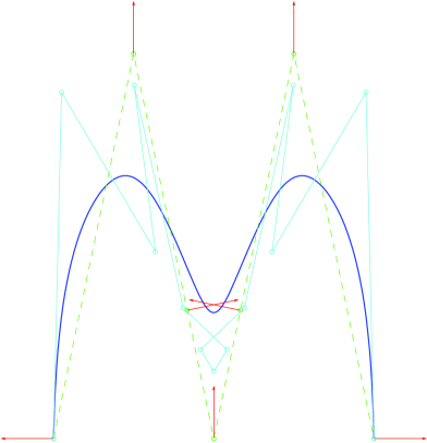
Figure 1: Conversion of a planar matrix weighted rational Bézier curve with point-normal control pairs into a rational Bézier curve.

3 Convert a matrix weighted rational Bézier curve to a rational Bézier curve in 3D

Suppose that $Q(t)$ given by Equation (1) is a matrix weighted rational Bézier curve lying in 3D space and the matrix function $M(t)$ is represented by its elements as

$$M(t)=\sum_{i=0}^{n}M_{i}B_{i,n}(t)=\left(\begin{array}[]{ccc}a_{11}(t)&a_{12}(t)&a_{13}(t)\\ a_{21}(t)&a_{22}(t)&a_{23}(t)\\ a_{31}(t)&a_{32}(t)&a_{33}(t)\end{array}\right).$$

Assume $A_{ij}(t)$ are the corresponding algebraic cofactors of elements $a_{ij}(t)$ of the matrix. We have

$$\begin{array}[]{ccc}A_{11}(t)&=&a_{22}(t)a_{33}(t)-a_{32}(t)a_{23}(t),\\ A_{12}(t)&=&a_{31}(t)a_{23}(t)-a_{21}(t)a_{33}(t),\\ A_{13}(t)&=&a_{21}(t)a_{32}(t)-a_{31}(t)a_{22}(t),\\ A_{21}(t)&=&a_{32}(t)a_{13}(t)-a_{12}(t)a_{33}(t),\\ A_{22}(t)&=&a_{11}(t)a_{33}(t)-a_{31}(t)a_{13}(t),\\ A_{23}(t)&=&a_{31}(t)a_{12}(t)-a_{11}(t)a_{32}(t),\\ A_{31}(t)&=&a_{12}(t)a_{23}(t)-a_{22}(t)a_{13}(t),\\ A_{32}(t)&=&a_{21}(t)a_{13}(t)-a_{11}(t)a_{23}(t),\\ A_{33}(t)&=&a_{11}(t)a_{22}(t)-a_{21}(t)a_{12}(t).\end{array}$$

By Equation (5), each $A_{ij}(t)$ can be formulated as a real function of degree $2n$ in terms of Bernstein bases. Then, the adjoint matrix is obtained as

$$\begin{array}[]{lll}M^{*}(t)&=&\left(\begin{array}[]{ccc}A_{11}(t)&A_{21}(t)&A_{31}(t)\\ A_{12}(t)&A_{22}(t)&A_{32}(t)\\ A_{13}(t)&A_{23}(t)&A_{33}(t)\end{array}\right)\\ &=&\sum_{i=0}^{2n}M_{i}^{*}B_{i,2n}(t)\end{array}$$

where $M_{i}^{*}$, $i=0,1,\ldots,2n$, are the coefficient matrices of order 3.

The real weights of the converted rational Bézier curve are derived by computing the determinant of the matrix $M(t)$. Assume that $a_{1l}(t)=\sum_{j=0}^{n}p_{lj}B_{j,n}(t)$, $A_{1l}(t)=\sum_{j=0}^{2n}q_{lj}B_{j,2n}(t)$, $l=1,2,3$. The determinant of the matrix $M(t)$ is formulated as

$$\begin{array}[]{lll}\det(M(t))&=&\sum_{l=1}^{3}a_{1l}(t)A_{1l}(t)\\ &=&\sum_{k=0}^{3n}\omega_{k}B_{k,3n}(t),\end{array}$$ (7)

where

$$\omega_{k}=\sum_{i+j=k,0\leq i\leq n,0\leq j\leq 2n}\frac{C_{n}^{i}C_{2n}^{j}\sum_{l=1}^{3}p_{li}q_{lj}}{C_{3n}^{k}}.$$

Similar to the conversion of matrix weighted rational Bézier curves in 2D, the control points of the converted rational Bézier curves in 3D are derived by computing the numerator in Equation (4). Denote $\bar{P}_{i}=M_{i}P_{i}$, $i=0,1,\ldots,n$. The numerator of the rational Bézier curve is formulated as

$$\sum_{i=0}^{2n}M_{i}^{*}B_{i,2n}(t)\sum_{j=0}^{n}\bar{P}_{j}B_{j,n}(t)=\sum_{k=0}^{3n}\omega_{k}Q_{k}B_{k,3n}(t)$$

where

$$Q_{k}={\frac{1}{\omega_{k}}}\sum_{i+j=k,0\leq i\leq 2n,0\leq j\leq n}\frac{C_{2n}^{i}C_{n}^{j}M_{i}^{*}\bar{P}_{j}}{C_{3n}^{k}}.$$

Finally, the converted rational Bézier curve is

$$Q(t)=\frac{\sum_{k=0}^{3n}\omega_{k}Q_{k}B_{k,3n}(t)}{\sum_{k=0}^{3n}\omega_{k}B_{k,3n}(t)}.$$ (8)

Figure 2 illustrates a spatial matrix weighted rational Bézier curve of degree 6 with point-tangent control pairs. In particular, the first three point-tangent control pairs and the last three point-tangent control pairs are lying on two planes that are perpendicular with each other while the middle point-tangent control pair lies on the intersection line between the two planes. The weight matrices of the curve are computed by Equation (3) with all $\omega_{i}=1$ together with $\mu_{0}=\mu_{6}=1.0$, $\mu_{1}=\mu_{5}=2.0$ and $\mu_{2}=\mu_{3}=\mu_{4}=4.0$. By applying the techniques discussed in Section 3, the original curve has been converted to a rational Bézier curve of degree 18. The solid cyan polygon in Figure 2 illustrates the control polygon of the rational Bézier curve.

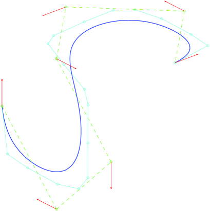
Figure 2: Conversion of a matrix weighted rational Bézier curve with point-tangent control pairs in 3D space into a rational Bézier curve.

4 Conjecture and closure

One main motivation for converting a matrix weighted rational Bézier curve to a conventional rational Bézier curve is to compute the convex hull of the curve. A sufficient condition for computing the convex hull of a rational Bézier curve by its control points is that all the weights are positive. All the examples we have experimented show that the converted rational Bézier curves do have positive weights, but the result is still difficult to prove at present. We therefore give the result as a conjecture.

Conjecture 4.1.

Assume a matrix weighted rational Bézier curve is defined by Equation (1) with weight matrices given by Equation (2) or (3). The real weights computed by Equation (5) or (7) are positive and the convex hull of the original matrix weighted rational Bézier curve can be computed by the convex hull of the control points of the converted rational Bézier curve.

Besides a theoretical proof of the conjecture, investigation of some other simple and effective algorithms for computing the convex hulls of matrix weighted rational Bézier curves is another interesting future work. As products of B-splines can be finally represented by B-splines, see for example (Chen et al., 2009), matrix weighted NURBS curves can be converted to conventional NURBS curves in the same way as the conversion of matrix weighted rational Bézier curves. Alternatively, a matrix weighted NURBS curve can first be decomposed into piecewise matrix weighted rational Bézier curves and then be converted to a spline of rational Bézier curves by the method discussed in this paper.

References

• Chen et al. (2009) Chen, X., Riesenfeld, R. F., Cohen, E., 2009. An algorithm for direct multiplication of b-splines. IEEE Trans. Automation Science and Engineering 6 (3), 433–442.
• Farin (2001) Farin, G., 2001. Curves and Surfaces for CAGD: A practical guide (Fifth Edition). Morgan Kaufmann.
• Farouki and Rajan (1988) Farouki, R. T., Rajan, V. T., 1988. Algorithms for polynomials in Bernstein form. Computer Aided Geometric Design 5 (1), 1–26.
• Sánchez-Reyes (2009) Sánchez-Reyes, J., 2009. Complex rational Bézier curves. Computer Aided Geometric Design 26 (8), 865–876.
• Yang (2016) Yang, X., 2016. Matrix weighted rational curves and surfaces. Computer Aided Geometric Design 42, 40–53.
• Yang (2018) Yang, X., 2018. Fitting and fairing Hermite-type data by matrix weighted NURBS curves. Computer-Aided Design 102, 22–32.