3D1D hydro-nucleosynthesis simulations. I. Advective-reactive post-processing method and its application to H ingestion into He-shell flash convection in rapidly accreting white dwarfs

Abstract

We present two mixing models for post-processing of 3D hydrodynamic simulations applied to convective-reactive $i$-process nucleosynthesis in a rapidly accreting white dwarf (RAWD) with $\mathrm{[Fe/H]}=-2.6$, in which H is ingested into a convective He shell. A 1D advective two-stream model adopts physically motivated radial and horizontal mixing coefficients constrained by 3D hydrodynamic simulations. A simpler approach uses diffusion coefficients calculated from the same simulations. All 3D simulations include the energy feedback of the $\mathrm{{}^{12}C}$$(p,\gamma)$$\mathrm{{}^{13}N}$ reaction from the H entrainment. Global oscillations of shell H ingestion in two of the RAWD simulations cause bursts of entrainment of H and non-radial hydrodynamic feedback. With the same nuclear network as in the 3D simulations, the 1D advective two-stream model reproduces the rate and location of the H burning within the He shell closely matching the 3D simulation predictions, as well as qualitatively displaying the asymmetry of the $X_{\mathrm{H}}$ profiles between the up- and downstream. With a full $i$-process network the advective mixing model captures the difference in the n-capture nucleosynthesis in the up- and downstream. For example, $\mathrm{{}^{89}Kr}$ and $\mathrm{{}^{90}Kr}$ with half-lives of $3.18\;\mathrm{\mathrm{min}}$ and $32.3\;\mathrm{\mathrm{s}}$ differ by a factor 2 - 10 in the two streams. In this particular application the diffusion approach provides globally the same abundance distribution as the advective two-stream mixing model. The resulting $i$-process yields are in excellent agreement with observations of the exemplary CEMP-r/s star CS31062-050.

1 Introduction

The details of mixing in convection zones within the stellar interior modifies the evolution of stars from the main sequence to the final white dwarf stage or supernova core collapse. The continual mixing of H into the convective cores of intermediate and massive stars sets a timescale for the eventual main-sequence turn off. This can be extended from convective boundary mixing which introduces additional H fuel to the core. Through this additional mixing of fuel into convection zones convective boundary mixing has a cumulative effect on the nuclear-time scale evolution of individual convection zones including on the mixture and amount of processed elements, the size of the convection zones and thereby on subsequent evolutionary phases (for example Herwig et al., 2000; Young et al., 2005; Denissenkov et al., 2012; Battino et al., 2016; Davis et al., 2019; Wagstaff et al., 2020).

Over the nuclear timescale of the H-burning during the main sequence, the mixing of chemical species is computed using either an instantaneous or diffusive mixing approximation. The nuclear burning timescale is usually significantly longer than the mixing timescale within the convective core leading to the details of the mixing within the convective zone being sufficiently well modeled with a space-time average theory. Such a theory, the mixing length theory (MLT Cox & Giuli, 1968), describes the energy transport and mixing properties of a convective region using averaged quantities over space and time. In advanced stages of stellar evolution the nuclear burning timescales approach convective timescales, and so the details of the mixing become increasingly important for their structure (Herwig et al., 2011b; Collins et al., 2018; Côté et al., 2020). To quantify this phenomenon, it is useful to define the Damköhler number, $\mathrm{Da}=\tau_{\mathrm{mix}}/\tau_{\mathrm{nuclear}}$, which is the ratio of the mixing and nuclear burning timescales. As this number becomes larger and closer to 1, the details of the mixing have a greater impact on the burning.

3D hydrodynamic simulations are becoming increasingly accurate in capturing the process of entrainment of fuel into a convection zone (Meakin & Arnett, 2007; Mocák et al., 2011; Woodward et al., 2015b) as well as the hydrodynamic feedback resulting from the dynamic nuclear burning of the ingested fuel (Meakin & Arnett, 2006; Herwig et al., 2014; Müller et al., 2016; Yoshida et al., 2019; Andrassy et al., 2019; Yadav et al., 2020). Such simulations predict how species are mixed into the convection zone and can determine the convective-reactive nucleosynthesis for a limited number of species without needing a post-processing. However, modeling any complicated nucleosynthesis, for example the $i$ process (Herwig et al., 2011a), or the detailed nucleosynthesis in the merger of a O and a C convection shell (Ritter et al., 2018a) may require networks with hundreds or thousands of species that can interact with each other, which is well beyond the capabilities of any 3D hydrodynamic code running on modern computing clusters. Therefore, 1D mixing models are still required to determine any complicated nucleosynthesis while 3D hydrodynamic simulations can be used to determine the mixing properties of the convection zone and how the hydrodynamic instabilities lead to the entrainment of stably stratified material. For example, the 3D hydrodynamic simulations of Ritter et al. (2018a) modeled a convective O shell with a stable C shell from a $15\,M_{\odot}$ stellar model of Ritter et al. (2018b) to obtain estimates for the expected entrainment rate of the C-rich material. Using diffusive mixing constrained by the mixing properties of the convection zone and appropriate entrainment rates, the 1D large-network nucleosynthetic post-processing models produced significant amounts of odd-Z elements like P, Cl, K and Sc, which could explain the underproduction of these elements in current GCE models (Ritter et al., 2018a). The nuclear network used in the 3D simulations only included the energy generation from the $\mathrm{{}^{12}C}$$(\mathrm{{}^{12}C},\alpha)$$\mathrm{{}^{20}Ne}$ and subsequent $\mathrm{{}^{16}O}$$(\alpha,\gamma)$$\mathrm{{}^{20}Ne}$ reaction.

An interesting case of convective-reactive nucleosynthesis occurs when H is ingested into a He burning convective shell. This triggers the $\mathrm{{}^{12}C}$$(p,\gamma)$$\mathrm{{}^{13}N}$ reaction and, after the $\mathrm{{}^{13}N}$ beta decays to $\mathrm{{}^{13}C}$, the $\mathrm{{}^{13}C}$$(\alpha,n)$$\mathrm{{}^{16}O}$ reaction can release neutrons if the temperatures within the He shell are high enough. Sakurai’s object (V4334 Sagittarii) has a unique surface chemical composition (Asplund et al., 1999) that can be explained with H being ingested into the He-shell flash convection zone of this post-AGB star (Herwig et al., 2011a). This results in the above chain of reactions and produces neutron densities high enough to be in the $i$-process regime ($N_{n}\approx 10^{12}-10^{16}$ cm^-3) (Cowan & Rose, 1977). The energy generation from this H ingestion can be significant enough to cause a split of the He convective zone in 1D stellar evolution models. To study the nucleosynthesis in Sakurai’s object, Herwig et al. (2011a) used a spherically symmetric diffusive mixing model based on MLT convective velocities, even though in those conditions several MLT assumptions are not satisfied. This is shown explicitly in the 3D hydrodynamic simulations of this very energetic event which bring about a global oscillation of shell H ingestion, that causes large-scale, non-radial and fast flows (Herwig et al., 2014).

A more quasi-static convective-reactive case of H-ingestion into a He shell has been found in the models of rapidly accreting white dwarfs (RAWDs) by Denissenkov et al. (2017). The 3D hydrodynamic simulations of Denissenkov et al. (2019) quantified the H-entrainment rates, however the diffusive mixing used in the post-processing was taken directly from the 1D stellar evolution models. The neutron densities in RAWDs reach $N_{n}\approx 10^{14}$ cm^-3 resulting in $i$-process nucleosynthesis. The RAWD heavy element production could result in a significant contribution of Kr, Rb, Sr, Y, Zr, Nb and Mo to the solar composition (Côté et al., 2018). The convective-reactive flows in RAWDs are fed by the $\mathrm{{}^{12}C}$$(p,\gamma)$$\mathrm{{}^{13}N}$ energy generation that comprises only $2-3\%$ of the total luminosity within the He shell which does not lead to a global oscillation of shell H ingestion (Denissenkov et al., 2019).

A solution to the concerns about the validity of diffusive mixing in a convective-reactive environment and the inability of 3D hydrodynamic simulations to simultaneously perform complex nucleosynthesis computations is to use a 1D advective mixing model. One such model has been adopted for use in the post-processing nucleosynthesis of stellar evolution models from the Monash group, MONSOON (Cannon, 1993; Henkel et al., 2017). The model contains two adjacent streams of fluid flow (see our Fig. 2 and Fig. 1 in Henkel et al., 2017), one with fluid moving upwards and another with fluid moving downwards. The two streams have an enforced horizontal mixing in order to conserve mass but it can also add in additional horizontal mixing. The radial transport velocities as well as the additional horizontal mixing within a convection zone are estimated with MLT.

A limitation in the two-stream methodology of MONSOON arises in the treatment of the additional horizontal mixing. The strength of this mixing has no dependence on the structure of the flow within the convection zone. Is the mixing between the two streams that represent the dominant dipolar flows of core convection the same as if the flow field was at smaller angular scales like in shell convection (Chandrasekhar, 1961)? There is a dependence on the horizontal mixing based on where a cell is within the convection zone but shouldn’t the mixing between the two streams, in low $\mathcal{M}a$ number flows, be stronger near the convective boundaries where the fluid is forced to overturn well before the convective boundaries (Jones et al., 2017)? These limitations are addressed in the advective mixing model of this work.

In this paper, we describe our adaptation of an advective two-stream model for post-processing of detailed 3D hydrodynamic simulations. We create 3D hydrodynamic simulations of a RAWD model from Denissenkov et al. (2019) to quantify the mixing of H into the He shell and to simulate the global flow including the energy feedback from nuclear burning of entrained material. After extracting the mixing information from the 3D hydrodynamic simulations for the 1D diffusive  (Jones et al., 2017) and advective mixing models, the time evolution of the H burning in both of them is calculated. The details of the 3D hydrodynamic simulations, as well as the diffusive and advective mixing approaches are outlined in Section 2. Section 3 discusses the flow properties of the simulations and shows the post-processing of the 3D hydrodynamic simulations with the diffusive and advective mixing routines. Section 4 describes the implications of such results and further applications.

2 Methods

2.1 PPMstar simulations

Table 1: Summary of the PPMstar simulations that were computed for this work. The entrainment rates are the slopes of the linear fits shown in Fig. 9, while the different definitions of the convective boundary are discussed in detail in Sections 3.1.2 and 3.2.

Run ID	Grid	$t_{\mathrm{sim}}\,(\mathrm{min})$	$\langle\tau_{\mathrm{conv}}^{i}\,(\mathrm{min})\rangle$	$L_{\mathrm{He}}\,(L_{\odot})$	$r_{\mathrm{b},\mathrm{SC}}^{ii}\,(\mathrm{Mm})$	$r_{\mathrm{b},v_{\perp}}^{iii}\,(\mathrm{Mm})$	$\sigma_{r_{\mathrm{b}},v_{\perp}}\,(\mathrm{Mm})$	$\dot{M}_{\mathrm{e}}^{iv}\,(M_{\odot}\,\mathrm{s}^{-1})$
N15	$768^{3}$	1634	19	$1.46\times 10^{8}$	$23.86$	$23.43$	$0.48$	$1.07\times 10^{-11}$
N16	$1536^{3}$	744	18	$1.46\times 10^{8}$	$23.84$	$23.56$	$0.46$	$7.21\times 10^{-12}$
N17	$1152^{3}$	631	9	$14.6\times 10^{8}$	$26.74$	$26.69$	$1.19$	$1.08\times 10^{-10}$

• Notes: ⁱ The average convective turn over time during the quasi-static phase of each run ($46<t<300\,\mathrm{min}$); ⁱⁱ The initial Schwarzschild boundary as followed in the Lagrangian coordinates at $t=299\;\mathrm{min}$; ⁱⁱⁱ Boundary where $\partial v_{\perp}/\partial r$ has a minimum at $t=299\;\mathrm{min}$; ^iv Entrainment rate of the H-rich fluid above the convection zone

The advective and diffusive post-processing methods introduced here are applied to 3D hydrodynamic simulations of He-shell flash convection in a rapidly accreting white dwarf (Denissenkov et al., 2017). The initial stratification has been taken from the stellar evolution model G with the metallicity [Fe/H] $=-2.6$ from Denissenkov et al. (2019).

As in previous work (Herwig et al., 2014; Jones et al., 2017) we use the PPMstar code of Woodward et al. (2015a) with additional details provided by Andrassy et al. (2019). The explicit Cartesian grid code is based on the Piecewise-Parabolic Method (PPM; Woodward & Colella, 1981, 1984; Colella & Woodward, 1984; Woodward, 1986, 2007), and tracks the advection of concentrations in a two-fluid scheme using the Piecewise-Parabolic Boltzmann method (PPB; Woodward, 1986; Woodward et al., 2015a).

The luminosity from the $\mathrm{{}^{4}He}$ burning within the convection zone is modeled with a constant volume heating. The entrained H reacts with the abundant $\mathrm{{}^{12}C}$ from the triple-$\alpha$ via the $\mathrm{{}^{12}C}$$(p,\gamma)$$\mathrm{{}^{13}N}$ reaction. This reaction rate is computed using the analytic form of the rate from Angulo et al. (1999) with no screening factor. We ignore the subsequent beta decay of $\mathrm{{}^{13}N}$ leaving a total energy release per reaction of $Q=1.943\;\mathrm{MeV}$. The stably stratified fluid above the convection zone contains 89.4% by number of H and the convective fluid contains 14.3% by number of $\mathrm{{}^{12}C}$. The PPMstar simulations done in this work are summarized in Table 1.

2.2 Diffusive mixing model

Jones et al. (2017) inverted the diffusion equation to derive a radius-dependent diffusion coefficient, which produces in 1D the same redistribution of species over the time frame of analysis as that given by their spherically-averaged 3D simulations of O-shell convection. They measured the rate of change in the radius-dependent mass fraction $X(r,\ t)$ of a species by computing the difference between the mass fraction profiles at two different points in time with some time averaging applied around them. With $\partial X/\partial r$ also known from the spherical averages, Jones et al. (2017) solve for the unknown diffusion coefficient, which we call $D_{\mathrm{FV}}(r)$, in the 1D Eulerian diffusion equation

$$\frac{\partial X}{\partial t}=\frac{\partial}{\partial x}\left(D_{\mathrm{FV}}(r)\frac{\partial X(r)}{\partial x}\right),$$

where they set $x=r$. We have improved upon this method by mapping the results of the input 3D Eulerian simulations to a mass coordinate $m(r)$ and inverting the Lagrangian diffusion equation

$$\frac{\partial X}{\partial t}=\frac{\partial}{\partial m}\left(\sigma(m)\frac{\partial X(m)}{\partial m}\right)+\frac{\dot{q}}{\rho},$$ (1)

where $\sigma=(4\pi r^{2}\rho)^{2}D_{\mathrm{FV}}(r)$ is the Lagrangian diffusion coefficient, and $\dot{q}(m,\ t)$ is the destruction rate of the species by nuclear reactions. This new approach has the following advantages. It removes the effect of thermal expansion and contraction from $\partial X/\partial t$. This effect has negligible influence on the results of Jones et al. (2017), but it is essential to account for in the expanding convection zone in these RAWD simulations. It also properly takes into account the spherical geometry of the problem with the radial dependence of the density and species. Included in our RAWD simulations but not in the O-shell convection simulations of Jones et al. (2017) are nuclear reactions between species of the two distinct fluids containing H and $\mathrm{{}^{12}C}$.

In order to invert equation 1 we need to take the difference of two averages of the fractional volume profiles, or – in this case – the mass fraction profile $X(r,\ t)$. For that we estimate the time in which it takes to diffuse across one mixing length:

$$\Delta t=\frac{(\alpha_{\mathrm{MLT}}H_{\mathrm{P}})^{2}}{4D_{\mathrm{FV}}}$$

where we take $H_{\mathrm{P}}$ and $D_{\mathrm{FV}}$ at the radius where $D_{\mathrm{FV}}$ is at its maximum. This diffusive timescale is $\Delta t\approx 2.5\;\mathrm{\mathrm{min}}$.

PPMstar simulations output a dump every several thousand time steps. For example in N16 every $\approx 2121$ time steps, where each time step is $\approx 1.3\times 10^{-2}\;\mathrm{\mathrm{s}}$, a single dump is output. For each dump at time $t_{\mathrm{D}}$, $D_{\mathrm{FV}}(r)$ is determined based on two profiles, $X(r,\ t_{\mathrm{D}}\pm\Delta t)$, each being averaged over $\Delta t$.

Despite taking the burning term into account in equation 1, the profile of the entrained material cannot be completely recovered, and thus the method cannot provide a diffusion coefficient in the lower part of the convection zone where all of the entrained material is burned (top panel Fig. 1).

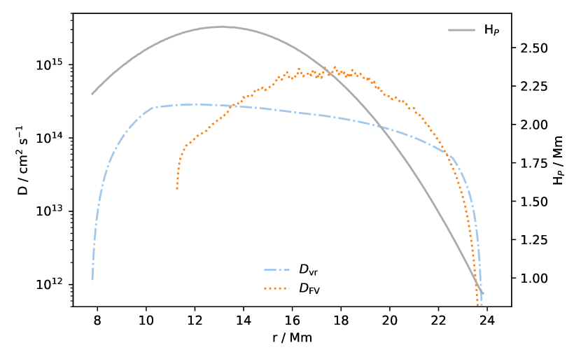
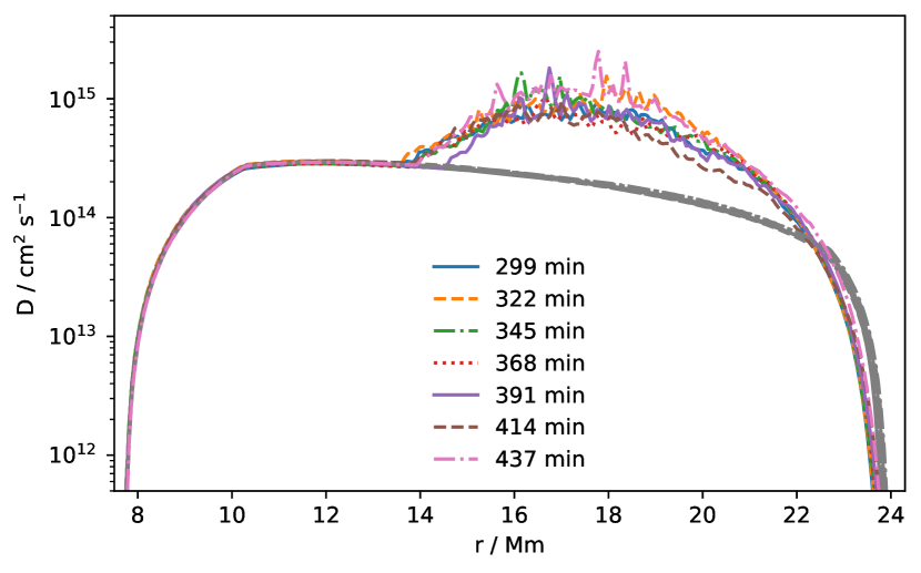
Figure 1: Top: $D_{\mathrm{vr}}$ according to equation 2, and $D_{\mathrm{FV}}$ according to the direct determination from the $X_{\mathrm{H}}$ profiles as well as the pressure scale height at $t=299\;\mathrm{min}$. Bottom: $D_{\mathrm{vr}}$ (grey lines) and the composite $D_{\mathrm{FV+vr}}$ (colour lines) according to the direct determination from the $X_{\mathrm{H}}$ at various times, merged with $D_{\mathrm{vr}}$ in the lower part of the convection zone (see text for details).

Therefore we also determine the diffusion coefficient from the spherically averaged radial velocity $v_{\mathrm{PPM}}$ from the 3D hydrodynamic simulation using the correction for the near-boundary regions recommended by Jones et al. (2017) based on O-shell simulations

$$D_{\mathrm{vr}}=\frac{1}{3}v_{\mathrm{PPM}}\times\min\left(l,|r-r_{0}|\right),$$ (2)

where $v_{\mathrm{PPM}}$ is the rms of the radial velocity on spherical shells from the 3D PPMstar simulation of the He-shell convection, $l=\alpha_{\mathrm{MLT}}H_{P}$ is the mixing length, and $|r-r_{0}|$ is the distance to the He-shell or another convective boundary that is located at the radius $r_{0}$. For $\alpha_{\mathrm{MLT}}=1.6$, this prescription provides the best fit to the diffusion coefficient derived from the hydrodynamic simulations of O-shell convection simulations (see Figure 21 in Jones et al., 2017). However that diffusion coefficient recommendation was focused on the behaviour of mixing near and across the top convective boundary (CB), and no attempt was made to model the discrepancy between the diffusion coefficient determined from the spherically averaged 3D hydrodynamic abundance profile evolution and the diffusion coefficient determined according to equation 2. This is clearly seen at the middle of the convection zone, $r=5.5\;\mathrm{Mm}$, in Figure 21 of Jones et al. (2017). In the RAWD case the burning of entrained H-rich material takes place approximately in the middle of the convection zone where this difference between $D_{\mathrm{vr}}$ and $D_{\mathrm{FV}}$ is largest ($\approx 0.4\dots 1.2\;\mathrm{dex}$, Fig. 1).

Where we are able to determine $D_{\mathrm{FV}}$ it is the more accurate diffusion coefficient that describes the underlying evolution of the spherically averaged 3D hydro profiles of these simulations better, for obvious reasons. In order to be able to use this more accurate diffusion coefficient we combine it in the lower half with the values of $D_{\mathrm{vr}}$ according to equation 2. We determine the radius $r_{\mathrm{Dmax}}$ where $D_{\mathrm{FV}}$ has its maximum. Then

$$D_{\mathrm{FV+vr}}=\begin{cases}D_{\mathrm{FV}},&\text{if }r>r_{\mathrm{Dmax}},\\ max(D_{\mathrm{FV}},D_{\mathrm{vr}}),&\text{otherwise}.\end{cases}$$

2.3 Advective mixing model

The 1D advection is formulated using a two-stream approach in which one stream transports species radially upwards, while the other stream transports them radially downwards (Cannon, 1993; Henkel et al., 2017, Fig. 2). Our adaptation of this advective two-stream (ATS) model to post-processing of 3D hydrodynamic simulations constitutes a reduced-dimensionality 1.5D advection model.

By default, the two streams are taken to be equal in their surface areas which is justified by the analysis of the 3D flow properties (see Section 3.1.1) and the discussion in Section 2.3.2. The model can have horizontal mixing between up- and downstream cells that are adjacent to each other.

There are $N$ cells per stream. The index $i$ refers to the spatial index of the $2N$ cells and is used where the equations are agnostic to whether the cell is within an up- or downstream. For computational and numerical simplicity, the indexing is done such that the downstream is inverted and stitched onto the top of the upstream. The indexing starts at the bottom of the upstream at $i=1$ and so cell $i=N+1$ is at the top of the downstream. The index $k$ refers to species.

The discretization distinguishes variables defined on the cell boundaries which have spatial half-integer indices, $i+1/2$, while those that represent cell averages have spatial integer indices $i$.

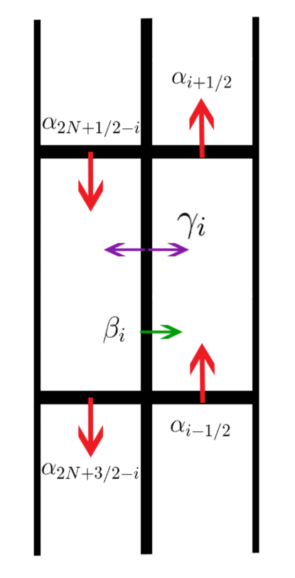
Figure 2: An illustration of the two-stream model including all of the fluxes for a cell within the convection zone; $\alpha$ the radial mass flux (Section 2.3.2), $\beta$ the enforced horizontal mass flux and $\gamma$ the additional horizontal mass flux (Section 2.3.3). The index $i$ refers to the upstream cell which has an adjacent downstream cell $2N+1-i$.

2.3.1 Discretized equations

To formulate the equations we start off with the conservation of mass equation and then apply the divergence theorem to it to yield

$$\partial_{t}\int_{V}\rho\mathrm{d}V=-\oint_{\partial V}\rho\vec{v}\cdot\mathrm{d}\vec{a}$$ (3)

The term on the right hand side is interpreted as a sum of mass fluxes through the boundary of the given volume, $V$. The term on the left hand side is the rate of change of the mass contained within that volume, $V$. This advective model conserves the total mass of every cell which requires that the sum of all mass fluxes at every cell is zero. Recasting equation 3 into the partial densities of every species, integrating both sides and applying the constraint that the mass of every cell is constant at all times leads to

$$\partial_{t}\left(\sum_{k}m_{k,i}\right)=-(\sum_{k}\sum_{j=1}^{5}F_{k,i}^{j})=0$$ (4)

where the index $j$ refers to a specific species mass flux on the surface of cell $i$. The mass, $m_{k,i}$, of a given species within a cell can change however the total mass within that cell cannot. This is implicitly satisfied with equation 4. Therefore these equations only transport the mass of a given species throughout the convection zone. Equation 4 includes all fluxes in the advective model and it is integrated explicitly.

2.3.2 Radial mixing and boundary conditions

Within the convection zone, the bulk transport of species is through the radial direction. The radial mass flux, $\alpha$, on each cell’s boundary is given by

$$\alpha_{i+1/2}=2\pi r^{2}_{i+1/2}\rho_{i+1/2}v_{i+1/2}$$ (5)

where $r$, $\rho$, $v$ are the radius, density and velocity defined on a cells boundary. The velocity is a positive-definite quantity in this model; the species mass fluxes will explicitly carry the appropriate sign for transport. In order for this model to remain consistent with the nearly-hydrostatic equilibrium of the underlying 3D stellar hydrodynamic simulation, the net mass flux at every radius must be zero to ensure that there is no net mass transport in the radial direction. This means that

$$\alpha_{i+1/2}=\alpha_{2N+1/2-i}$$ (6)

In equation 5, the radial mass flux depends on a surface area, taken to be $2\pi r^{2}$, to which the underlying transport of mass, $\rho v$, is advected through. In principle, the surface area can be different between the up- and downstream cells and still ensure that the net mass flux is zero so long as the product $\rho v$ with the respective surface areas are constant at every radius. With the low $\mathcal{M}a$ number flows in the RAWD simulations, the largest density perturbations are at the percent level as seen in Fig. 4. The density can therefore be approximated to be constant at every radius so that $\rho_{i+1/2}=\rho_{2N+1/2-i}$. The spherical average of the radial velocity at every radius is approximately zero (Fig. 4). The magnitude of the velocity at the surface of the up- and downstream cells at each radius can then be approximated as being the same, $v_{i+1/2}=v_{2N+1/2-i}$. With the density and velocities being equal in both streams at a given radius, the surface areas of each stream must also be equal to ensure that there is no net radial mass transport. Another consequence of these approximations is that the mass of the cells in both streams at a given radius are also equal, $\delta m_{i}=\delta m_{2N+1-i}$.

The radial species mass fluxes for cell $i$ are

$$F_{k,i}^{O} =\alpha_{i+1/2}X_{k,i+1/2}$$ (7a)

$$F_{k,i}^{I} =-\alpha_{i-1/2}X_{k,i-1/2}$$ (7b)

where the superscript $O$ and $I$ refer to the outflow and inflow of mass at cell $i$, respectively. These constitute two of the fluxes from equation 4. The mass fractions, which are defined in the center of a cell, $X_{k,i}$, are considered the average within that cell. To achieve second order accuracy in the solutions of these equations, the mass fraction on a boundary, $X_{k,i+1/2}$, is determined through a linear interpolation using the neighbouring cell averages. There are two estimates for the interpolated state,

$$X_{k,i+1/2} =X_{k,i+1}-\frac{1}{2}\frac{\partial X_{k,i+1}}{\partial m_{i+1}}\delta m_{i+1}$$

$$X_{k,i+1/2} =X_{k,i}+\frac{1}{2}\frac{\partial X_{k,i}}{\partial m_{i}}\delta m_{i}$$

referring to the up-sided and down-sided estimates of the interpolated mass fraction, respectively. To ensure that the numerical scheme is stable, the interpolated state is chosen such that the discretization is upwinding. In practice, this just means that if the velocity is upwards, the upwinded interpolated state is the down-sided estimate because material is being advected upwards. To reduce oscillations in the solutions the minmod limiter is used on the numerically estimated slope (LeVeque, 2002).

$$\frac{\partial X_{k,i}}{\partial m_{i}}=\texttt{minmod}(\frac{X_{k,i}-X_{k,i-1}}{\delta m_{i}},\frac{X_{k,i+1}-X_{k,i}}{\delta m_{i}})$$

where

$$\texttt{minmod}(a,b)=\left\{\begin{array}[]{lr}a&\text{if }|a|<|b|\text{ and }a\cdot b>0\\ b&\text{if }|b|<|a|\text{ and }a\cdot b>0\\ 0&\text{otherwise}\end{array}\right.$$

At the inner and outer boundaries of the convection zone the velocities are zero. Physically, this condition is enforcing that all of the radial flow is turning over at the boundary such that there is only a horizontal flow. Of course, fluid can and does over turn at some distance before the boundary (Jones et al., 2017) which are written as sources of horizontal mixing in this model (Section 2.3.3). The constraints on the radial mass flux coefficients to enforce a horizontal flow at the boundaries are

$$\alpha_{N-1/2}=\alpha_{N+1/2}=\alpha_{N+3/2}$$

$$\alpha_{2N-1/2}=\left(\alpha_{2N+1/2}\equiv\alpha_{1/2}\right)=\alpha_{3/2}$$

These coefficients cause, at the uppermost cell in the upstream, all of the mass that enters that cell to flow directly into the uppermost cell in the downstream. This is a horizontal flow. These boundary conditions are essentially periodic boundary conditions and from the numerical and computational perspective, it is convenient to have the two streams attached to each other to form a ring. By applying equation 3 to a convection zone that has zero velocity on its boundaries, there is no mass entering or leaving the convection zone and so it remains constant. For this reason, the model follows the Lagrangian coordinates of the PPMstar initialized convection zone as it expands in Eulerian coordinates (Section 3.1.2).

2.3.3 Horizontal mixing

With only the radial mass fluxes given by equation 7 contributing to equation 4 thus far, the only way in which the fluxes at the upper and lower boundary of any cell sum to zero is if the product of $2\pi r^{2}\rho v$ is constant for all radii. This is not true for the convection zone in the RAWD simulations nor in general. Rather, the rms radial velocity profile from the 3D simulations in Fig. 3 shows a pronounced peak about 1/3^rd from the bottom of the convection zone and falls off well inside the CBs where the flow turns around in a broad sweep corresponding to the low $\mathcal{M}a$ numbers.

Using Fig. 2 as a reference, if the upstream has $\alpha_{i+1/2}>\alpha_{i-1/2}$, then over a time step the mass within that cell $i$ will decrease. Simultaneously the downstream will be increasing its mass by the same amount due to the radial mass fluxes being equal in the two streams at every radius (equation 6). To conserve the mass in each of the cells, there is an enforced horizontal mass flux of

$$\beta_{i}=\alpha_{i+1/2}-\alpha_{i-1/2}$$ (10)

from one stream to the other. The sign of this coefficient $\beta$ determines whether mass is transferred from the downstream to the upstream or vice versa. The horizontal species mass flux at the upstream cell with index $i$ is

$$F^{\beta}_{k,i}=\left\{\begin{array}[]{lr}-|\beta_{i}|X_{k,2N+1-i}&\text{if }\beta_{i}>0\\ |\beta_{i}|X_{k,i}&\text{if }\beta_{i}<0\end{array}\right.$$

One could consider a situation where neighboring cells at the same radius conserve mass in the shell but allow for the mass in each cell to be variable so that the $\beta$ coefficient is not exactly as written in equation 10. However, since the density fluctuations are at the percent level as shown in Fig. 4 they are approximated as being the same between the two streams at every radius. Therefore the mass within each cell should not change due to horizontal mixing. Combining this fact with there being no net radial transport of mass, the mass within every cell is constant at all times.

With the $\beta$ and $\alpha$ mass fluxes, the total mass flux at every cell is zero. There can be additional horizontal mass fluxes so long as the sum of them is equal to zero. This additional horizontal mass flux is given the symbol $\gamma$ and it is unique within each shell, i.e $\gamma_{i}=\gamma_{2N+1-i}$, to ensure that the total mass flux at every cell is still zero. However, the additional horizontal species mass flux is not zero and has the form

$$F^{\gamma}_{k,i}=\gamma_{i}\left(X_{k,i}-X_{k,2N+1-i}\right)$$ (11)

for each cell.

While mass is being transported radially in the up- and downstreams, mass is also being exchanged between them through a horizontal mass flux. The mixing of the mass of a given species $k$ between cell $i$ and its adjacent cell $2N+1-i$ implied by equation 11 has the effect of homogenizing the species between the two streams at every layer, depending on the value of $\gamma$. There are two competing timescales that determine how efficient the mixing between the up- and downstreams are. These are the radial advection timescale,

$$\delta t_{r,i}=\frac{|\delta r_{i}|}{v_{r,i}}$$ (12)

and the horizontal time scale, $\delta t_{h,i}$, for a given cell. Associated with these timescales are mass fluxes. The radial mass flux is $\alpha$, while the horizontal mass flux is $\gamma$. With these two competing timescales, if one is shorter than the other then it is implied that the shorter timescale has a larger mass flux than the longer timescale. This can be written as

$$\gamma_{i}=\alpha_{i}\frac{\delta t_{r,i}}{\delta t_{h,i}}$$ (13)

The mental picture of a convection zone being composed of one upstream and one downstream that splits the convection zone evenly into two hemispheres is very unrealistic (Fig. 4). Instead, this model should be thought of as the upstream being the superposition of all radially upward flows and similarly for the downstream. From this idea, if the upward flows are small in their surface area at a given radius, they can more easily mix with the adjacent downward flows. To decompose the velocity into upward and downward flows at a particular length scale on a sphere, the power spectrum (spherical harmonics) of the radial velocity is taken. To compute the spherical harmonics the python package pyshtools is used for data sampled on a sphere. The maximum mode, $\ell$, that the velocity field is decomposed into is chosen such that the smallest wavelength, $\lambda=2\delta r$ where $\lambda=2\pi r/\sqrt{\ell(\ell+1)}$, that can be sampled from the briquette data (see Fig. 4 and Section 3.1) with a grid spacing of $\delta r$ is computed.

For a given mode, $\ell$, there is an associated length scale, or wavelength. A particle at the center of a stream must move, tangentially to the surface of the sphere, half of this wavelength to be in the center of the adjacent stream. With an average tangential velocity, the particle will take $\delta t_{h,i,\ell}=\pi r_{i}/\left(\langle|v_{\perp,i}|\rangle\sqrt{\ell(\ell+1)}\right)$ amount of time to mix, for a given mode $\ell$. The flow does not develop with only one very dominant mode but a spectrum of modes (Fig. 5) and so the horizontal timescale is weighted by its power, $S_{cc}(\ell,r)=\sum_{m=-\ell}^{\ell}|c_{\ell,m}(r)|^{2}$. Therefore, the horizontal timescale is

$$\delta t_{h,i}=\sum_{\ell}\frac{S_{cc}(\ell,r_{i})\pi r_{i}}{\left(\sum\limits_{\ell}S_{cc}(\ell,r_{i})\right)\langle|v_{\perp,i}|\rangle\sqrt{\ell(\ell+1)}}$$ (14)

2.3.4 Entrainment

A convection zone can entrain, or ingest, material due to hydrodynamic instabilities at the boundaries. In the RAWD simulations, the fluid above the convection zone is entrained into the convection zone through a downstream at the convective boundaries, as shown in Fig. 4, bringing H-rich material into the convection zone. With the constraint on the advective model that the mass within any cell cannot change, the mass of the fluid above the convection zone that is entrained into a cell must also be removed. Algorithmically, the entrainment process follows what was discussed in detail in Appendix A of Denissenkov et al. (2019). The H-rich material is ingested into the downstream into a region of mass, $\Delta M$, that is equal to the mass of the top cell of the downstream. This ensures that all of the mass that is entrained is done so directly through the convective boundary surface, thus incorporating the horizontal and radial mixing timescales to determine how fast the composition changes are transported downwards. Due to $\Delta M$ being only one cell, the change in the mass fractions is applied as a step increase.

To test how well entrainment and mixing is modeled we have switched off all reactions and compared the total amount of H ingested into the top cell with the amount of H distributed over the other cells by mixing. The relative difference between these amounts in the advective model remains within $2-4\%$ even after 30334 time steps ($744\;\mathrm{min}$ of integration time). In the diffusive model the entrained material is distributed evenly over 18 cells (out of a total number of 256 cells) using the step increase method from Appendix A of Denissenkov et al. (2019). Over the same number of time steps as the advective model we find that the relative differences between the total entrained H and the mixed H in the diffusive model to be of the same order, $2-4\%$.

2.3.5 The Courant Condition

With the fact that the method is explicit, the time steps are limited by the Courant condition. With the cells being discretized in mass, the Courant condition can be plainly stated as requiring that the total amount of mass advected out of any given cell in a single time step cannot be larger than the mass within that cell. The Courant number in any cell is given by

$$C_{i}=\frac{\delta t\left(\alpha_{i+1/2}+\gamma_{i}+|\beta_{i}|\right)}{\delta m_{i}}$$ (15)

and the Courant condition states that for all $i$, $C_{i}\leq 1$. Any advective post-processing simulations have the condition that the maximum Courant number across all cells is $0.5$. This determines the time steps that any post-processing model takes (see Section 3.2).

2.4 mppnp post-processing simulations

The 1D multi-zone NuGrid code, mppnp (Pignatari et al., 2016; Ritter et al., 2018b), is used for the 1D post-processing models of the PPMstar simulations. Either the diffusive or advective mixing routine, as described in Sections 2.2 and 2.3 respectively, is used for a given mppnp simulation which are tabulated in Table 2. The first set of runs has been performed by including only the $\mathrm{{}^{12}C}(p,\gamma)\mathrm{{}^{13}N}$ reaction rate and neglecting its electron screening, just as in the PPMstar runs, in order to have a direct comparison between 1D and 3D. The second set of runs has been performed with a full network of $\sim$1000 species suitable for $i$-process simulations in which we use the same nuclear data and electron screening factors as in Denissenkov et al. (2019). Both the advective and diffusive mixing post-processing models, for a given 3D PPMstar run, use the same spherically averaged radial $\rho$, $T$ profiles and time steps corresponding to the 3D dump times. The details of the formulation of the models are discussed in Section 3.2.

Table 2: Summary of the 1D mppnp post-processing simulations.

mppnp Run ID	A/Di	Hydro Run ID	Networkii
mp1	$D_{\mathrm{FV+vr}}$	N16	$\mathrm{{}^{12}C}(p,\gamma)\mathrm{{}^{13}N}$
mp2	ATS	N16	$\mathrm{{}^{12}C}(p,\gamma)\mathrm{{}^{13}N}$
mp3	$D_{\mathrm{vr}}$	N17	$\mathrm{{}^{12}C}(p,\gamma)\mathrm{{}^{13}N}$
mp4	ATS	N17	$\mathrm{{}^{12}C}(p,\gamma)\mathrm{{}^{13}N}$
mp5	$D_{\mathrm{FV+vr}}$	N16	full
mp6	ATS	N16	full
mp7	$D_{\mathrm{vr}}$	N17	full
mp8	ATS	N17	full
mp9	$D_{\mathrm{vr}}$	N16	$\mathrm{{}^{12}C}(p,\gamma)\mathrm{{}^{13}N}$
mp10	$D_{\mathrm{vr}}$	N16	full

• ⁱ The mixing model used in the post-processing which is either diffusive ($D_{\mathrm{vr}}$ or $D_{\mathrm{FV+vr}}$, Section 2.2) or advective (ATS, Section 2.3); ⁱⁱ $\mathrm{{}^{12}C}(p,\gamma)\mathrm{{}^{13}N}$ indicates post-processing with the same one-reaction burn that is implemented in the PPMstar runs, full indicates post-processing with the complete network needed for $i$-process modeling

3 Results

We first describe the hydrodynamic simulations of RAWDs in Section 3.1. The details of the post-processing models are discussed in Section 3.2. Focusing on the only nuclear reaction included in the hydrodynamic simulation we then describe and compare post-processing via the diffusive (Section 3.3.1) and advective methods (Section 3.3.2). In Section 3.4 we describe the post-processing results including a full network and comparison with observations.

3.1 3D hydrodynamic simulations of RAWDs

3.1.1 Flow properties

As with the other PPMstar simulations in Woodward et al. (2015a); Jones et al. (2017); Andrassy et al. (2019), the RAWD simulations do not start with any initial perturbations in the velocity field but rather the numerical representation of the spherically symmetric thermodynamic variables develop instabilities. These are quickly over taken by the flow developing from heat being injected (Table 1) in a thick spherical shell. This shell is contained within the radii $8.28\;\mathrm{Mm}$ and $10.28\;\mathrm{Mm}$ and can be seen as the beige shaded region in Fig. 3. After about 30 minutes this transient state is completely lost in the simulations and the natural flow of the convection zone has developed.

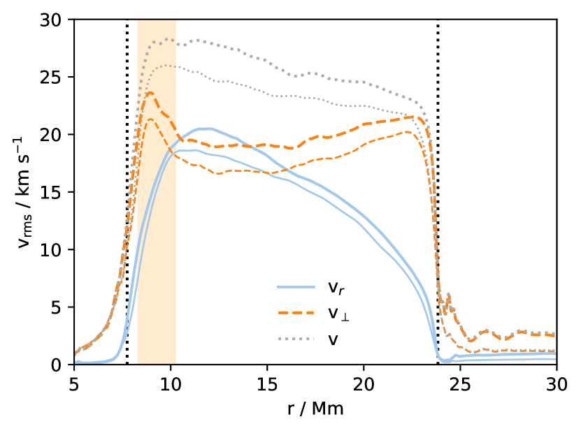
Figure 3: The rms radial profiles of $v_{r}$, $v_{\perp}$ and $v$ at $t=299\;\mathrm{min}$. The thick lines are from run N16, while the thin lines are from run N15. The black dotted lines correspond to the convective boundaries that are used in N16’s post-processing models (Sections 3.1.2 and 3.2). The beige shaded region is where the volume heating is applied. When spatially integrated it corresponds to the helium luminosity, $L_{\mathrm{He}}$, stated in Table 1.

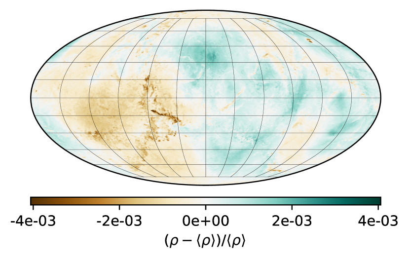
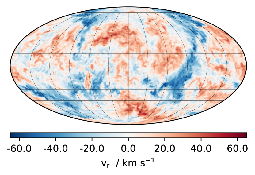
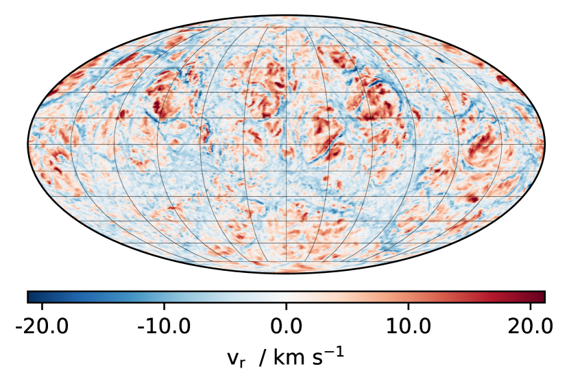
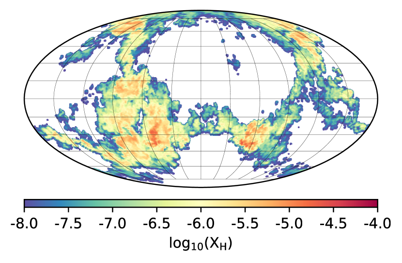
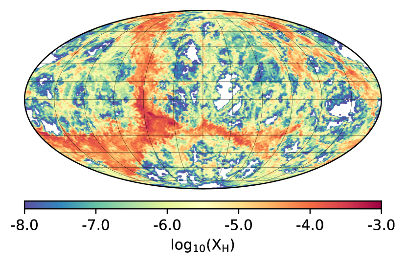
Figure 4: In each row the left panel is a Mollweide plot of the quantity at a radius of $14.5\;\mathrm{Mm}$, which is within the H burning region (Fig. 15), while the right panel is at a radius of $23\;\mathrm{Mm}$ which is near the top CB (Table 1). The first row plots the density perturbations from its mean, the second row plots the radial velocity, while the last row plots the mass fraction of H which is calculated from the FV that is at double the grid resolution. The Mollweide plots were made with the briquette data which is downsampled by a factor of 4 (384³) from the resolution of the underlying run, N16 (1536³), and are taken at $t=299\;\mathrm{min}$. The points on the shell to which the quantity is sampled on are distributed such that each point’s surface area coverage is roughly equal to $4\pi/N$. The number of points that are used roughly corresponds to having a single point per cubic cell.

The rms radial profiles of the radial and tangential velocities are shown in Fig. 3. The radial velocity drops sharply near the CBs, while the tangential velocity is dominant near the CBs. Directly from these profiles it is clear that there will be significantly more horizontal mass transport near the CBs (equation 13) than the middle of the convection zone. This coincides with the flows being forced to turn over near the CBs. N15’s spherically averaged velocities are smaller than N16’s and it is significant when considering that the difference between the two runs is the doubling of the spatial resolution in N16. A possible cause for this is due to the higher entrainment rates in N15 compared to N16, shown in Fig. 9. With the convective fluids doing work to bring the initially stable fluid above the convection zone into the convection zone, some of its kinetic energy is lost resulting in the lower velocities.

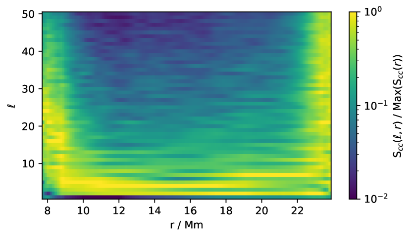
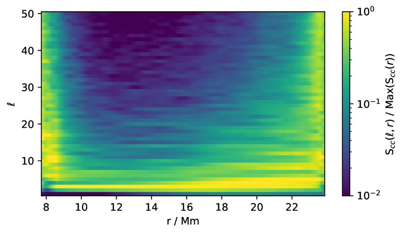
Figure 5: The power spectrum, in terms of the spherical harmonic modes, $\ell$, of the radial velocity as a function of radius at $t=299\;\mathrm{min}$ within the convection zone. The left panel is from run N15, while the right panel is from run N16. The power in each radial bin is normalized by the maximum power within that radial bin.

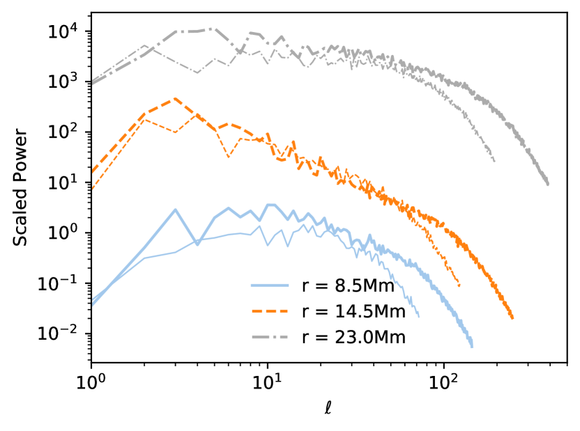
Figure 6: The power spectrum of the radial velocity as a function of the spherical harmonic mode, $\ell$, at select radii at $t=299\;\mathrm{min}$. The thick lines are run N16, while the thin lines are from run N15. The spectrum is limited by the Nyquist sampling of the briquette data resulting in more $\ell$ modes being resolved in the higher resolution run, N16. The power in each spectrum at a given radius is scaled by an arbitrary constant factor, which is the same for each hydro run, in order to show their $\ell$ dependence clearly.

The radial velocity field is shown at two radii in Fig. 4. These Mollweide-projection plots are made using the briquette data from a PPMstar simulation. This data set is downsampled in each spatial direction by a factor of four from the original simulation through averaging the data in 4³ cells. The radial velocity at $14.5\;\mathrm{Mm}$ is mostly dominated by two modes, $\ell=2$ and $3$, which can be seen visually in Fig. 4 as well as from its power spectrum in Figs. 5 and 6. This is consistent with the flow being dominated by the most unstable and largest convective mode that can be in that spherical shell, $\ell\approx\pi r/\Delta r\approx 3$ (Chandrasekhar, 1961). At $23\;\mathrm{Mm}$, the velocity field is not dominated by a few modes but the power is instead spread over many modes of $\ell$. The large plumes that are advecting from the center of the convection zone are broken up into smaller, incoherent streams that are swept across by the large tangential velocities (Figs. 3 and 7).

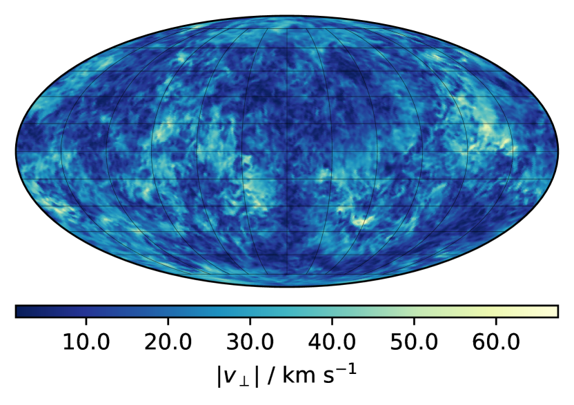
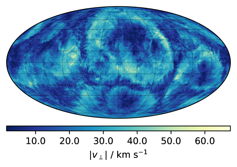
Figure 7: The magnitude of the tangential velocity, $|v_{\perp}|=\sqrt{v_{\phi}^{2}+v_{\theta}^{2}}$, on spherical shells from N16. The left panel is at a radius of $14.5\;\mathrm{Mm}$, within the H burning region (Fig. 15), while the right panel is at a radius of $23\;\mathrm{Mm}$ which is near the upper convective boundary (Table 1). These snapshots are taken at $t=299\;\mathrm{min}$.

3.1.2 The convective boundary and entrainment and burning of H

The CB in 1D stellar evolution models can be determined by the Schwarzschild criterion. If the fluid is unstable to convection and is fully mixed within the convection zone, it is adiabatically stratified such that $dS/dr=0$, or in the case of an ideal gas equation state, which is used for the simulations done in this paper, it can be expressed as $dA/dr=0$ where $A=P/\rho^{\gamma}$ with $\gamma=5/3$. The PPMstar simulations are initialized with a convection zone defined by these properties. The CB can be determined throughout the entirety of the simulation by assuming that the convection zone is only expanding due to heat and so it can be determined directly by using the Lagrangian coordinates of the initial Schwarzschild boundary. This initial Schwarzschild boundary is determined numerically with the condition that fluid with $dA/dr>0$ is stably stratified. In previous works that used the PPMstar code (Jones et al., 2017; Andrassy et al., 2019; Denissenkov et al., 2019) the CB during the simulation was determined using the minimum of $\partial v_{\perp}/\partial r$ with the spherically averaged profiles of $|v_{\perp}|$ or with the bucket data of $v_{\perp}$ (see Section 3.3 in Jones et al. (2017)). The Schwarzschild criterion does not adequately describe the stability of the fluid near the boundaries in these simulations as even in areas where the entropy gradient is weakly positive, the fluid is flowing with moderate velocities (Jones et al., 2017). The gradient condition expresses the 3D nature of the CB as when the fluid advects near the stiff boundary, the fluid is forced to turn over. This can be viewed as small perturbations from a spherically symmetric boundary as shown in Fig. 8. The thickness of this CB as described by 1$\sigma$ spatial fluctuations (Fig. 17 in Jones et al., 2017) is approximately $0.5\;\mathrm{Mm}$, which is smaller than the pressure scale height at that boundary, $H_{P}=1.0\;\mathrm{Mm}$. The CB as determined by the minimum of $\partial v_{\perp}/\partial r$ as well as the CB defined by the Lagrangian coordinates of the initial Schwarzschild boundary for all runs at $t=299\;\mathrm{min}$ are tabulated in Table 1. A discussion on the appropriate boundary for the mppnp post-processing models is within Section 3.2.

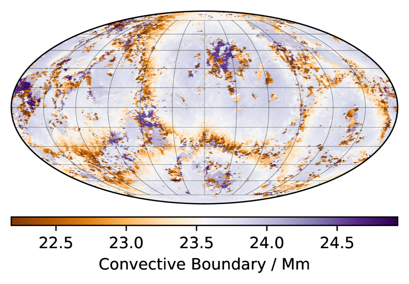
Figure 8: Location of the upper convective boundary of N16 according to the minimum of $\partial v_{\perp}/\partial r$ at $t=299\;\mathrm{min}$ from the briquette data. Taking the spherical average, the upper convective boundary is at $23.56\;\mathrm{Mm}$ with $\sigma_{r_{\mathrm{b}},v_{\perp}}=0.46\;\mathrm{Mm}$. This is consistent with the other CB determination which uses the mass coordinates of the initial Schwarzschild boundary to yield an upper CB at $23.84\;\mathrm{Mm}$.

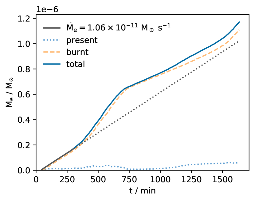
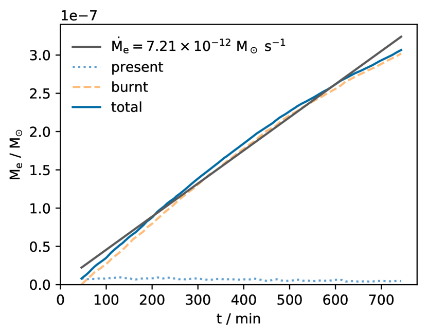
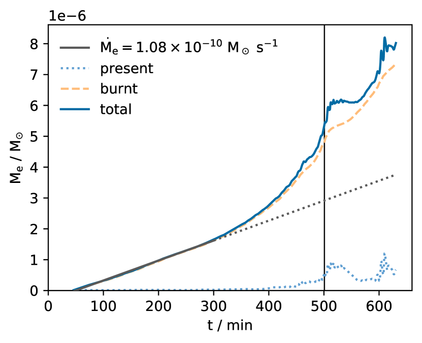
Figure 9: The time evolution of the mass of the fluid above the convection zone being entrained and burned within the convection zone since the start of the mppnp post-processing models, $t=46\;\mathrm{min}$. The top panel is from N15, the middle panel is from N16 and the bottom panel is from N17. The total lines is the instantaneous entrainment rate of the fluid above the convection zone which is used in all advective and diffusive post-processing models. A linear fit of the entrainment rates, $\dot{M}_{\mathrm{e}}$, for each run is calculated over a quasi-static time interval corresponding to the solid line, while the dotted line is an extension of that fit. The black vertical line is at $t=501\;\mathrm{min}$ when the images of Fig. 11 were rendered.

At the upper CB, the entrained fluid above the convection zone follows the convective downflows deep into the convection zone until it reaches the burning region where the $\mathrm{{}^{12}C}$$(p,\gamma)$$\mathrm{{}^{13}N}$ reaction occurs. To determine the entrainment rates of N15, N16 and N17, a method, which is described in more detail in Andrassy et al. (2019) and Denissenkov et al. (2019), was used. To summarize, the total mass of the fluid above the convection zone that was entrained is composed of the mass that has been burned and the mass that is present within the convection zone with an upper boundary radius of $r_{\mathrm{ub}}$. To determine the mass of the fluid above the convection zone within this convection zone its density is integrated to within $0.5\;\mathrm{Mm}$ of the formal CB of the mppnp post-processing simulations (see Section 3.2). This offset is approximately the average scale height of the rms tangential velocity gradient at the boundary, $H_{v_{\perp},\mathrm{ub}}=(\partial\>\mathrm{ln}\>v_{\perp}/\partial r)^{-1}$, a condition used in Jones et al. (2017), Andrassy et al. (2019), and Denissenkov et al. (2019), for all RAWD simulations during their quasi-static burning phases. The constant offset prevents major fluctuations in the calculated entrained mass due to the very large concentrations of the fluid above the convection zone near the CB and prevents major changes in the velocity field (global oscillation of shell H ingestion in N15 and N17; see Section 3.1.3) from providing outlandish integration boundaries. This offset is extended to $5\;\mathrm{Mm}$ for N17 during its global oscillation of shell H ingestion due to the major changes in the spherically averaged fluid above the convection zone concentrations near the majorly perturbed convective boundary. The burnt material is calculated using the spherical profiles of density, temperature and mass fraction to determine what the burning rate per unit volume is. This burning rate is integrated in time to determine the amount burnt over a dump. The entrainment rates, mass burnt, and present material of the fluid above the convection zone within the CBs of N15, N16 and N17 are shown in Fig. 9. A linear fit of the entrainment rate of N15, N16, and N17 over their quasi-static burning phases are $\dot{M}_{\mathrm{e}}=1.06\times 10^{-11}\,M_{\odot}$ s^-1, $\dot{M}_{\mathrm{e}}=7.21\times 10^{-12}\,M_{\odot}$ s^-1, and $\dot{M}_{\mathrm{e}}=1.08\times 10^{-10}\,M_{\odot}$ s^-1, respectively. N15 and N17’s entrainment rates become non-linear and increases significantly around $t=300\;\mathrm{min}$ (Fig. 10). Even within the linear regime the entrainment rate of N15 is $\approx 10\%$ larger than N16’s though the scale of this difference is consistent with the entrainment convergence results in Fig. 17 of Woodward et al. (2015a).

Throughout the entirety of the N16 simulation, the burning and entrainment of H maintains a quasi-static state resulting in the linear growth of the total entrained material. The distribution of $X_{\mathrm{H}}$ is plotted on spherical shells near the upper CB, $23\;\mathrm{Mm}$, and well within the H burning region, $14.5\;\mathrm{Mm}$, in Fig. 4. The corresponding radial velocity field at those radii is shown in Fig. 4. The distribution of the $X_{\mathrm{H}}$ at $14.5\;\mathrm{Mm}$ in conjunction with the radial velocity distribution shows that that the upflows are essentially H-free while the downflows are H-rich. As the H-rich material moves through the H burning region, the downflow material is rapidly burned until it is H-free. Eventually this material will turn around and move in the upflows entirely H-free. The H-free material is advected and mixed with the H-rich material as it is advected towards the upper boundary where it still maintains very small mass fractions ($X_{\mathrm{H}}\approx 10^{-6}$) at $23\;\mathrm{Mm}$, $\approx 0.8\;\mathrm{Mm}$ from the upper CB (Table 1). The H-rich material ($X_{\mathrm{H}}\approx 10^{-3}$) is advected into the convection zone in the downflows near the CB.

3.1.3 A global oscillation of shell H ingestion in N15 and N17

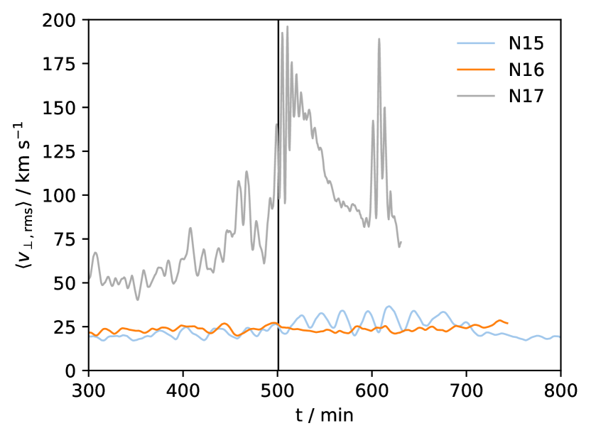
Figure 10: The average of the rms tangential velocity between 1 and $2\;\mathrm{Mm}$ below each simulations top Schwarzschild boundary as described in Section 3.1.2. The very large oscillations in the tangential velocity in N17 indicate a global oscillation of shell H ingestion is occurring which causes the entrainment rate to increase by up to a factor of 80 (see Fig. 9) during these oscillations. Much milder oscillations can be seen in N15 between 500 and $700\;\mathrm{min}$ with a modest factor of 3 increase in its entrainment rate. The black line refers to the time when the images of FV in Fig. 11 were rendered.

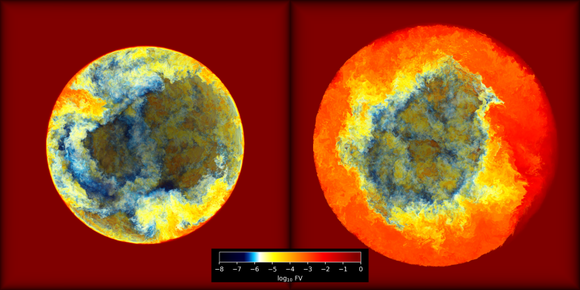
Figure 11: Both panels show a rendering of the fractional volume FV of the material in the stable layer at $t=501\;\mathrm{min}$. The C-rich convective fluid is transparent. The left panel is from N16, while the right panel is from N17. The entrainment rate of H rapidly increases when a global oscillation of shell H ingestion instability occurs in N17. The hydrodynamic feedback from the energy released from burning causes even more H to be entrained and leads to an unstable runaway in N17 but not in N15. This is contrasted with the quasi-static entrainment and burning in N16 (Fig. 9).

Directly from the entrainment rates of each run in Fig. 9, the entrainment rates begin to increase substantially around $t=300\;\mathrm{min}$ in both N15 and N17 and continues until $t\approx 700\;\mathrm{min}$. N17’s entrainment rate increases by a factor of up to 80 during this time compared with its quasi-static rate, while N15’s entrainment rate increases by a factor of up to 3. The cause of these bursts of entrainment are due to the collision of opposing horizontal flows forcing significant amounts of H-rich material to be entrained in downdrafts where it will eventually burn and feedback energy into the flow (Herwig et al., 2014). The magnitude of the horizontal oscillations of these flows is clearly seen in Fig. 10 where the rms of the tangential velocity rapidly increases and decreases within convective turn over timescales. With the same heating rate as N15, N16 does not undergo a global oscillation of shell H ingestion at any point during its entire simulation which includes the full duration of the global oscillation of shell H ingestion experienced by N15.

The consequences of the global oscillation of shell H ingestion between N15 and N17 differ drastically due to the differences in the amount of H ingested. The weak global oscillation of shell H ingestion of N15 does not entrain enough H to sustain it for a long period of time and thus it dissipates after $200\;\mathrm{minutes}$ of large scale oscillations. The burning of this additional entrained H is done such that there is very little build up of H within the convection zone (Fig. 9) during the global oscillation of shell H ingestion. The global oscillation of shell H ingestion does not increase the average tangential velocity significantly over its duration and a global oscillation of shell H ingestion does not occur again throughout the $1600\;\mathrm{minute}$ long simulation. Conversely, N17’s global oscillation of shell H ingestion causes significantly higher entrainment of H which is built up within the convection zone. This can be seen in the rendering of the fractional volume, FV, at $t=501\;\mathrm{min}$ in Fig. 11. The global oscillation of shell H ingestion subsides briefly after the large build up of H and burns most of the H within the convection zone and then begins again at $t=600\;\mathrm{min}$. The simulation is ended soon after the global oscillation of shell H ingestion continues again as the expansion of the convection zone has approached where the outer boundary condition is applied.

3.2 mppnp post-processing model constraints

Due to the initial transient at the start of any PPMstar simulation, the mppnp post-processing models do not begin until well after this transient has finished. This was chosen to be at $46\;\mathrm{minutes}$ for N16 and N17. The advective mixing models are initialized with an $X_{\mathrm{H}}$ profile in the up- and downstreams that is equivalent to the spherically averaged $X_{\mathrm{H}}$ profile from the PPMstar simulation. The diffusive mixing model is initialized with the spherically averaged $X_{\mathrm{H}}$ profile from the PPMstar simulation. For the advective post-processing it is not expected that the up- and downstreams would have equivalent $X_{\mathrm{H}}$ profiles as seen in Fig. 4. While running, the initial guess of the equivalent profiles in the up- and downstreams is quickly changed to the model’s preferred profile which is asymmetric (see Fig. 14). This takes around 3 convective turn over timescales and causes comparisons with PPMstar profiles to be inaccurate during this initialization period. For this reason, all mppnp post-processing models repeat the very first time step, with the entrainment rate at that point in time, for $\approx 3$ convective turn over timescales so that they establish their own quasi-static profile.

The PPMstar simulations output the briquette, and any other data type, on a dump basis. The advective mixing models have their time steps being limited by a Courant condition, equation 15, which requires on the order of 20-30 time steps being taken for every single dump of N16. Although the implicit solving of the diffusion equation used by mppnp is not limited to a time step criterion like the advective mixing model, all post-processing models for a given run, regardless of mixing or network, use the advective mixing models Courant condition limited time steps. Both the advective and diffusive post-processing models, for a given 3D PPMstar run, use the same spherically averaged radial $\rho$, $T$ and $v_{\mathrm{rms}}$ profiles at a dump. Although the stratification and velocity profiles do change throughout a dump it is negligible as the convective turn over time is $\approx 1100\;\mathrm{s}$ for N16, while the dump interval is $\approx 27\;\mathrm{s}$.

As discussed in Section 3.1.2, the CBs in 3D hydrodynamic simulations are not a sharp and spherically symmetric boundary as typically interpreted with the Schwarzschild criterion. The minimum of the spherical average of $\partial v_{\perp}/\partial r$, which can define the location of the CB, could be used to determine a time dependent CB for the post-processing models. However, with this CB varying at each dump in the Eulerian coordinates it is also varying in its mass coordinates. Because the advective mixing model requires that the mass of the individual cells to remain constant across all time (Section 2.3) this boundary determination can cause the upper and lower boundaries to sporadically move between cells on a dump basis. During a global oscillation of shell H ingestion this boundary determination can lead to a top boundary well within the convection zone, as it was determined before it began to global oscillation of shell H ingestion, due to the large oscillations in the tangential velocities (see Fig. 10). To simplify the definition of the CB and make it applicable to all runs, instead the mass coordinates of the initial Schwarzschild boundaries are used to define the convective boundaries for all post-processing models. The difference between the two boundary criteria is only $0.43\;\mathrm{Mm}$ at $t=299\;\mathrm{min}$ for N16 (Table 1). Given that the determination of the tangential velocity gradients are from the briquette data, which is downsampled from the PPMstar simulation and only have a cell length of $0.18\;\mathrm{Mm}$, and the fact that $\sigma_{r_{\mathrm{b}},v_{\perp}}=0.46\;\mathrm{Mm}$ for that averaged boundary the two boundary determinations are mostly in agreement.

The mass coordinates of the cell interfaces, which are constant for the whole duration of the post-processing, are calculated by initially splitting the convection zone into equally spaced radial shells in the Eulerian coordinates. This makes the mass of individual cells to vary radially but this ensures that the sampling of data from the hydro simulations is done at the cell resolution. There are approximately $250$ cells for the post-processing models of N16 and N17. The number of cells in N16 was reduced due to the computational effort required when using a full network. As the PPMstar simulation evolves in time, the density, velocity and radius are interpolated to the mass coordinates of the cell interfaces.

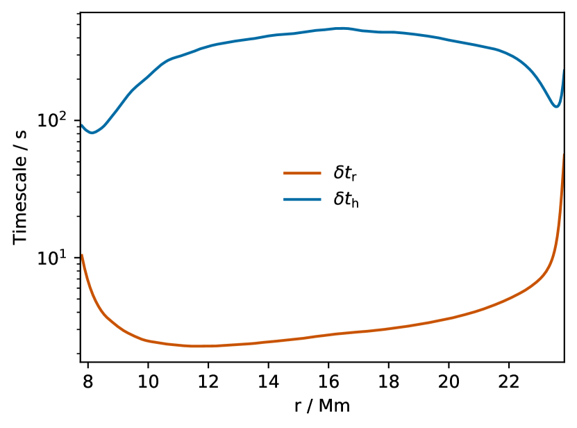
Figure 12: The radial and horizontal mixing timescales as a function of radius within the convection zone at $t=299\;\mathrm{min}$ for run N16. Equations 12 and 14 define the radial and horizontal mixing timescales, respectively.

The stream model for N16 was run from $t=46\;\mathrm{min}$ until the end of that simulation at $t=744\;\mathrm{min}$ resulting in roughly 39 convective turn over times. The entrainment of the fluid above the convection zone into the convection zone of the post-processing models is taken directly from the time dependent entrainment in Fig. 9. The entrainment rates are small enough that the fact that the mass of the convection zone does not change over the length of the post-processing model is an accurate approximation to the PPMstar simulations. Integrating N16’s entrainment rate over the length of its simulation results in a total of $3.1\times 10^{-7}\,M_{\odot}$ of fluid above the convection zone being entrained. The cell with the smallest mass within the advective post-processing models of N16 is $2.6\times 10^{-6}\,M_{\odot}$.

3.3 $\mathrm{{}^{12}C}(p,\gamma)\mathrm{{}^{13}N}$-only post-processing models

3.3.1 Diffusive post-processing models

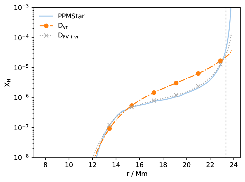
Figure 13: The $X_{\mathrm{H}}$ profiles from N16 and from post-processing models mp9, using $D_{\mathrm{vr}}$ according to the recipe provided in Jones et al. (2017), and mp1, using $D_{\mathrm{FV+vr}}$ which inverts the diffusion equation using the spherically-averaged $X_{\mathrm{H}}$ profiles of PPMstar as described in Section 2.2.

Using spherical averages of the $X_{\mathrm{H}}$ and rms of the radial velocity from PPMstar the diffusion coefficients $D_{\mathrm{vr}}$ and $D_{\mathrm{FV+vr}}$ are computed on a dump basis. Using these diffusion coefficients in mppnp with only the $\mathrm{{}^{12}C}(p,\gamma)\mathrm{{}^{13}N}$ reaction, the post-processing models of mp1 and mp9 are compared with PPMstar in Fig. 13. Unsurprisingly, the model using the $D_{\mathrm{FV+vr}}$ matches the PPMstar profile very closely except right at the top CB. This is due to the accuracy of estimating the strength of the mixing and the calibration of the entrainment rates. By using the $D_{\mathrm{vr}}$ diffusion coefficient the mixing near the convective boundary is largely overestimated and the mixing near the middle is underestimated. Even though the $|r-r_{0}|$ term in equation 2 decreases as the boundary is being approached, $D_{\mathrm{vr}}$ does not fall off as quickly as the $D_{\mathrm{FV+vr}}$ profiles suggest in Fig. 1.

3.3.2 Advective post-processing models

From Figs. 5 and 6 the power spectra of N16 shows dominant large-scale modes at the middle of the convection zone as well as a more flat spectrum across many scales when near either CB. With the smaller modes contributing significantly to the power near the CBs the mixing between the two streams is expected to be more efficient there than the middle of the convection zone. Applying equation 14, the horizontal and radial timescales for run N16 are shown in Fig. 12. The horizontal timescale is typically over an order of magnitude larger than the radial timescale suggesting inefficient mixing, even at the CBs. There is still significant power at the largest modes near the CBs leading to small changes in the horizontal timescales across the entire convection zone. The lack of efficient horizontal mixing is especially apparent in the middle of the convection zone where the up- and downstreams are very isolated from each other as seen in Fig. 14. The upstream is carrying nearly H-free material towards the top of the convection zone, while the downstream is carrying H-rich material directly to the burning region. This distribution of H-free fluid in the upstream and H-rich fluid in the downstream is also validated by the 3D hydro simulations as seen in Fig. 4.

The spherical average of the X_H profiles from the two streams closely follows the spherical average of N16 in most regions. However, at the very top of the convection zone it is underestimated, while between 16 and $22\;\mathrm{Mm}$ it is overestimated, similarly to the results of the diffusive mixing with $D_{\mathrm{vr}}$ (Fig. 13). One component of this is likely due to an underestimation of the horizontal mixing at the top of the convection zone. The briquette data used to compute the spectra of the radial velocity has a resolution that is a factor of 4 smaller than the run’s grid resolution. This downsampling involves averaging which significantly dampens the power in any short wavelength modes, directly increasing the horizontal mixing timescale and leading to less efficient mixing. This results in much more efficient radial transport of species allowing for the sliver of very H-rich material at the top of the convection zone to immediately advect downwards rather than be constantly mixed between the two streams.

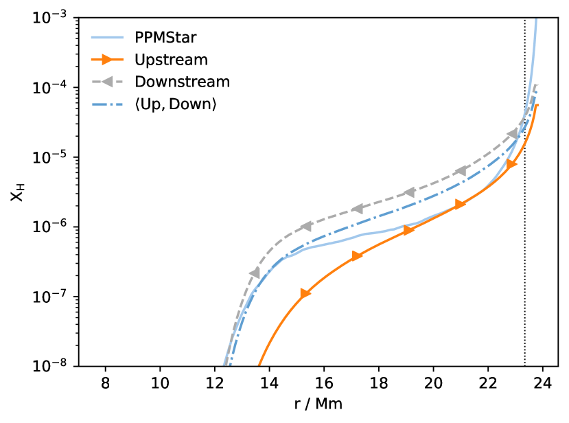
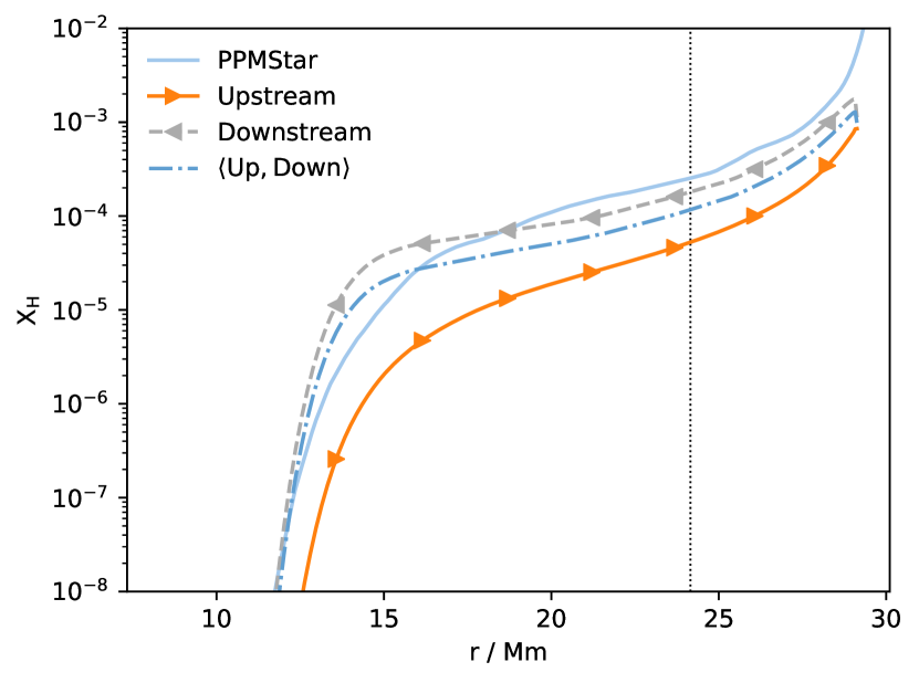
Figure 14: The top panel is the $X_{\mathrm{H}}$ profiles from N16 and the up- and downstreams of mp2 at $t=299\;\mathrm{min}$. The spherical average of the up- and downstreams is $\langle\mathrm{Up},\mathrm{Down}\rangle$. The bottom panel plots the same quantities for N17 and the post-processing model mp4 at $t=501\;\mathrm{min}$, during the global oscillation of shell H ingestion. The black vertical dotted line is where the integration of the fluid above the convection zone is stopped for calculating the entrainment rates in Fig. 9.

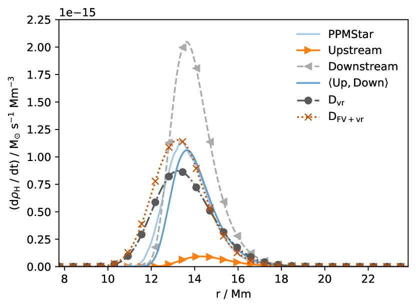
Figure 15: The burning rate of H per volume as a function of radius for N16, an advective post-processing model, mp2, and the diffusive post-processing models mp1 and mp9. The $\langle\mathrm{Up},\mathrm{Down}\rangle$ profile is calculated with the spherical average of the streams to estimate the burning rate, similarly to the estimates from spherically averaged data of PPMstar. The $\mathrm{{}^{12}C}$$(p,\gamma)$$\mathrm{{}^{13}N}$ reaction is very sensitive to temperature and it does not burn any H until about $18\;\mathrm{Mm}$ with $\mathrm{T9}=0.11$. All of the H is burned well before it reaches the bottom of the convection zone.

To better understand the physics of the convective-reactive nucleosynthesis in the RAWD model, it is useful to find out where the H-burning is predominately occurring within its He shell. The H burning rate at a single time step from the PPMstar simulations and the advective post-processing model, mp2, are estimated in N16 with the techniques discussed in Section 3.1.2 and is shown in Fig. 15. The advective post-processing model is burning the H a few cells above where N16 is burning H. This could suggest that the distribution of flow velocities that are present in PPMstar simulations modifies where the bulk of the burning takes place within a convection zone. With the fact that there is no significant accumulation of H throughout the advective post-processing model it is roughly in a quasi-static state in which it is burning all of the H that it ingests.

3.4 Full network post-processing and comparison with observations

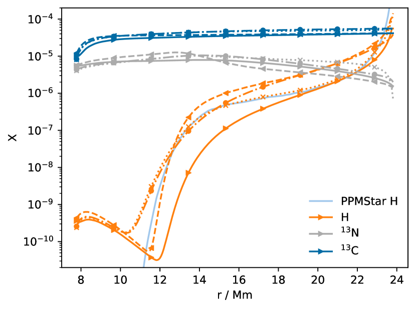
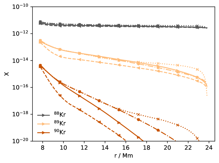
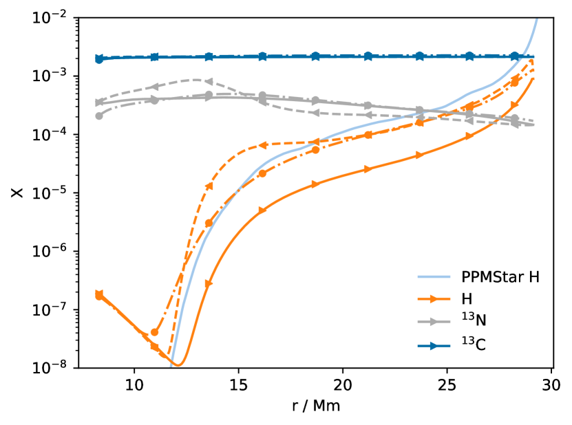
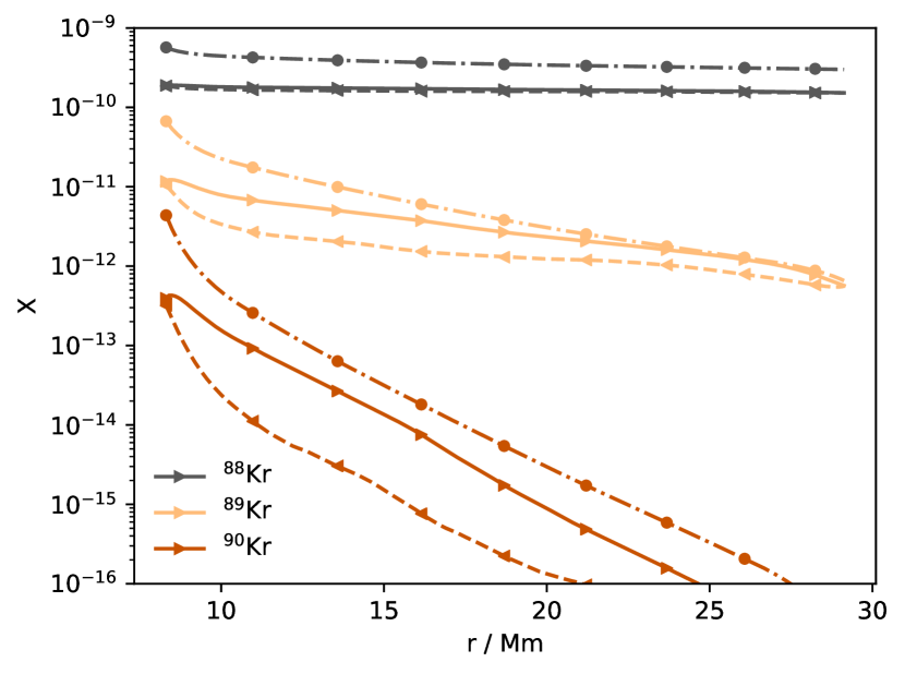
Figure 16: The top row contains panels using data from the post-processing models of mp5, mp6 and mp10 (N16) at $t=299\;\mathrm{min}$, while the bottom row contains panels using data from the post-processing models of mp7 and mp8 (N17) at $t=501\;\mathrm{min}$. In each row, the left panel contains line profiles of the mass fractions of H, $\mathrm{{}^{13}N}$, and $\mathrm{{}^{13}C}$, while the right panel contains line profiles of the mass fractions of various Kr isotopes. These isotopes are $\mathrm{{}^{88}Kr}$, $\mathrm{{}^{89}Kr}$, and $\mathrm{{}^{90}Kr}$ which have half lives of $2.84\;\mathrm{hr}$, $3.18\;\mathrm{minute}$ and $32.3\;\mathrm{s}$, respectively. The mixing models are distinguished based on line style and glyphs as was done in Figs. 13 and 14. $D_{\mathrm{vr}}$ profiles are dash-dotted with circles, $D_{\mathrm{FV+vr}}$ profiles are dotted with cross’, the upstream profiles are solid with a triangle pointing towards higher radii and the downstream profiles are dashed with a triangle pointing towards lower radii.

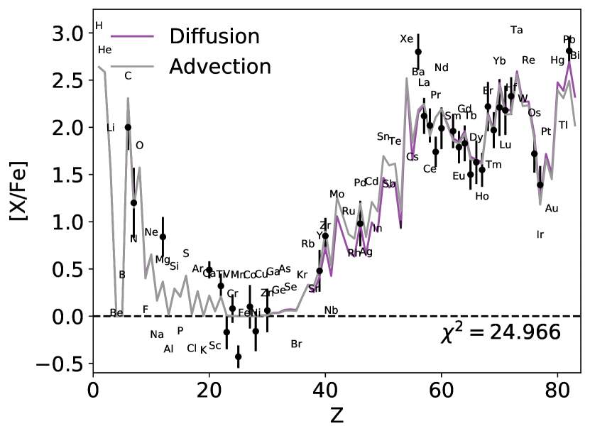
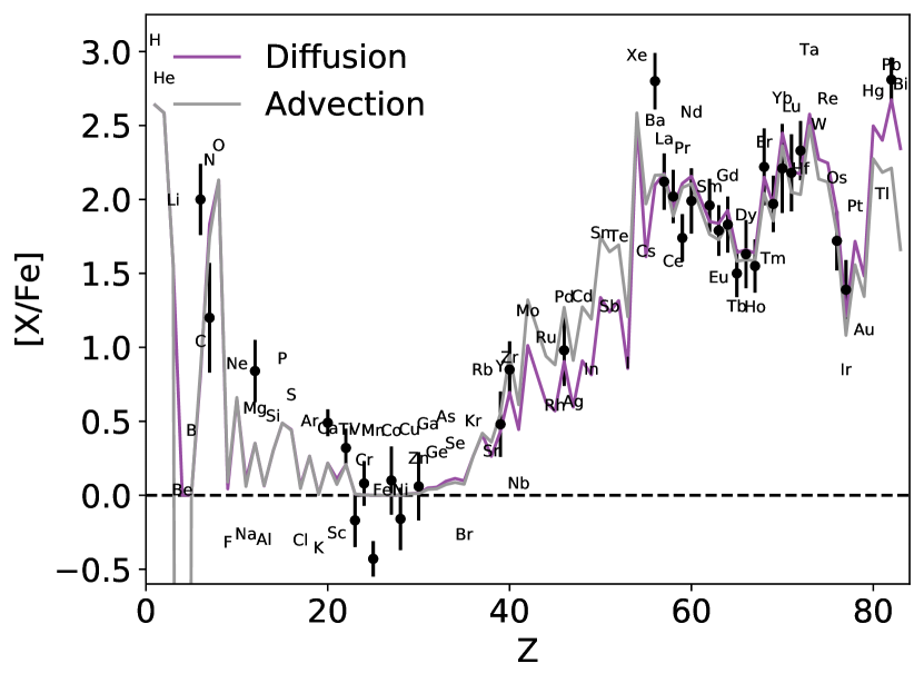
Figure 17: Both panels show an elemental abundance distribution of the best-fit time for a diffusive post-processing model (mp5 at 0.059 yr for N16 and mp7 at 0.017 yr for N17) with star CS31062-050 (Aoki et al., 2002; Johnson & Bolte, 2004) as well as the appropriate advective post-processing model at the same simulation time (mp6 for N16 and mp8 for N16). The top panel plots the models from run N16 with the lower $N_{\mathrm{n}}$ thus taking longer to reach the $\mathrm{Pb}$ elemental abundance than the bottom panel which uses models of N17. The abundances are scaled by the solar abundances from Asplund et al. (2009).

With the limitation of only having two fluids in the hydrodynamic simulations only the energy feedback from the $\mathrm{{}^{12}C}$$(p,\gamma)$$\mathrm{{}^{13}N}$ reaction can be modeled within them. The 1D advective and diffusive post-processing simulations that use the mixing and entrainment calibrated from those hydro simulations can model the $i$-process by incorporating a nuclear network with thousands of species. With the additional reactions there appear sources of neutrons and H at the bottom of the convection zone through the $\mathrm{{}^{13}C}$$(\alpha,n)$$\mathrm{{}^{16}O}$ and various $(n,p)$ reactions as seen in the left panels of Fig. 16. Although not very significant, there is a distinction between how the advective and diffusive mixing models behave with two burning regions for a given isotope. For N16, there is the H-burning region that ends roughly around $12\;\mathrm{Mm}$, where the $X_{\mathrm{H}}$ reaches a minimum, and then there is the H source from $(n,p)$ reactions that occurs until the bottom CB. The advective mixing model clearly distinguishes these two burning regions, while the diffusive mixing model smears them, even with time steps that are needed to resolve an explicit advective model. Of course, with larger time steps this smearing becomes much more significant and the profiles are not properly converged. Another important detail with the advective models is that up- and downstreams are distinct in not only H but other isotopes as well. As the H is advected down in the downstream it burns to produce $\mathrm{{}^{13}N}$ which has a half life of approximately $10\;\mathrm{min}$. In N16 the convective turn over timescale is $18\;\mathrm{min}$ leading to some of the $\mathrm{{}^{13}N}$ to decay as it moves to the bottom CB and then turns over into the upstream. This can also be traced with the $\mathrm{{}^{13}C}$ as it is burned while being advected by the downstream to the bottom CB. When it eventually moves upwards in the upstream more of the $\mathrm{{}^{13}N}$ decays and replenishes the burned $\mathrm{{}^{13}C}$, and the streams become homogenized.

On the right panels of Fig. 16 a few unstable Kr isotopes are plotted with varying half lives. With the convective turn over timescales of $18\;\mathrm{min}$ and $9\;\mathrm{min}$ for N16 and N17 respectively the long half life of $\mathrm{{}^{88}Kr}$, $2.84\;\mathrm{hr}$, ensures that it is well mixed as its Damköhler number ($\mathrm{Da}=\tau_{\mathrm{mix}}/\tau_{\mathrm{nuclear}}$) is much less than 1. However for $\mathrm{{}^{89}Kr}$ and $\mathrm{{}^{90}Kr}$, with their half lives of $3.18\;\mathrm{min}$ and $32.3\;\mathrm{s}$, their Damköhler numbers become greater than 1. With these isotopes the distinction between the up- and downstreams becomes apparent and important for describing their distribution within the convection zone. Again, the production of the neutrons and thus these unstable species is predominately at the bottom CB. They are produced when the appropriate $n-1$ isotope is advected down and then captures a neutron after which it will predominately be advected away in the upstream.

While the hydrodynamic simulations are only able to model the He-shell flash convection and the H ingestion for roughly half a day, the latter can last in RAWDs roughly for a month (Denissenkov et al., 2019). A simple approximation for modeling the $i$-process over that longer timescale is to assume that the quasi-static behavior of N16 will continue, and so the post-processing models are repeated to stretch the integration time. Likewise, the N17 simulated behavior can be repeated. The RAWD model G from Denissenkov et al. (2019), on which these simulations are based, had $i$-process yields that were in good agreement with the observed elemental abundance distribution in the exemplary carbon-enhanced metal poor (CEMP-r/s) star CS31062-050 with seemingly enhanced $s$-process and $r$-process material. There, a simpler approximation was used to compute the $i$-process yields in which a representative time step during the H-ingestion phase was used as a static model for mppnp with the diffusion coefficients provided by MESA (Denissenkov et al., 2019; Paxton et al., 2010). Fig. 17 shows the best fit in time of the decayed elemental abundance yields from mp5, and mp7, with the corresponding advective post-processing models mp6 and mp8, compared with the surface chemical composition of CS31062-050 from Aoki et al. (2002) and Johnson & Bolte (2004). Neither of the advective models has a large enough neutron exposure at that point in time to reach the $\mathrm{Pb}$ elemental abundances observed in that star. The difference in the time it takes for the advective model to reach the same $\mathrm{Pb}$ abundances as in the diffusive model is approximately 7%. This is of the same order as the inaccuracies in the amount of H ingested and mixed, therefore this is not due to differences in how the $i$-process nucleosynthesis works in the advective mixing models, but is likely due to the numerics (Section 2.3.4). From the many RAWD models of Denissenkov et al. (2019) it is clear that the neutron density is directly proportional to $\dot{M_{\mathrm{H}}}$ as nearly all of the ingested H is burned via $\mathrm{{}^{12}C}$$(p,\gamma)$$\mathrm{{}^{13}N}$ leading to a neutron being released. Therefore, the best fit is reached at an earlier time for the mp7 run that is based on the N17 simulations with the higher H-entrainment rate.

The important result is that even with using the advective method that models mixing in RAWDs closer to what is observed in 3D hydrodynamic simulations and uses much better time resolution we can still reproduce the observed chemical composition of CS31062-050 well within the H-ingestion timescale of 0.087 yr estimated from the 1D stellar evolution computations.

4 Summary and conclusions

In this paper, we described, formulated and applied two different numerical methods to model the mixing within a convection zone from 3D hydrodynamic simulations in order to compute convective-reactive $i$-process nucleosynthesis. The stellar environment of choice was the He shell in a RAWD with a metallicity of $\mathrm{[Fe/H]}=-2.6$ (model G of Denissenkov et al. (2019)). One method used a standard 1D diffusive mixing routine, while the other was a two-stream advective mixing model that is likened to the models of Cannon (1993) and Henkel et al. (2017). These models require mixing coefficients which could be taken from estimates using MLT however instead we constrain the mixing by running 3D hydrodynamic simulations of the RAWD. The mixing coefficients in both models are determined directly from the data of the 3D hydrodynamic simulations.

The high resolution RAWD simulation, N16, was run for approximately 39 convective turn over times showing that its evolution over this timescale to be approximately quasi-static. The radial velocity field at $14.5\;\mathrm{Mm}$ is dominated by the large modes of $\ell=2$ and $3$, while near the CBs the flow is spread across many smaller modes (Figs. 4 and 5). The large scale modes encounter the stiff upper boundary and begin to turn over, increasing the tangential velocities near the boundaries (Figs. 3 and 7). Using the gradient of the tangential velocity as a condition for the CB yields a spherically averaged boundary at $23.56\;\mathrm{Mm}$ at $t=299\;\mathrm{minutes}$. This CB is consistent with the CB as determined by the initial Schwarzschild boundary of the 3D simulations, which is followed in the Lagrangian coordinates, to within a standard deviation of that averaged boundary. This is roughly at the resolution of the briquette data that was used to calculate those boundaries.

The entrainment of fluid above the convection zone in N16 is linear in time with an entrainment rate of $\dot{M}_{\mathrm{e}}=7.21\times 10^{-12}\,M_{\odot}$ s^-1. N15’s entrainment rate increases by as much as a factor of 3 after it experiences a global oscillation of shell H ingestion however it returns to quasi-static burning and entrainment as shown in Fig. 9. The global oscillation of shell H ingestion instability in N17 causes it go into a feedback loop of rapidly increasing entrainment in which it does not return to quasi-static burning and entrainment. The entrained H-rich fluid is advected along the downflows to be burned rapidly at $14.5\;\mathrm{Mm}$, while the H-free fluid is advected along the upflows. These two fluid mixtures are nearly isolated from each other as there is a significant amount of H-free fluid with $X_{\mathrm{H}}\leq 1\times 10^{-6}$ very close to the upper boundary, $23\;\mathrm{Mm}$, while the spherical average is $X_{\mathrm{H}}\approx 1\times 10^{-3}$ in the PPMstar simulations.

The 1D mppnp post-processing simulations were first applied with only the $\mathrm{{}^{12}C}$$(p,\gamma)$$\mathrm{{}^{13}N}$ reaction which is the only reaction included in the PPMstar simulations. The instantaneous burning rate of H per unit volume is estimated in N16 and mp2 which are in good agreement as to where the bulk of the burning occurs. The up- and downstreams of mp2 have horizontal mixing timescales that are 1-2 dex longer than the radial mixing timescales resulting in the streams not homogenizing. Each stream has a distinct $X_{\mathrm{H}}$ radial profile that is qualitatively similar to N16’s distribution of H-free upflows and H-rich downflows though not of the same magnitude. The spherical average of the two streams is consistent with the PPMstar $X_{\mathrm{H}}$ profiles except at the upper boundary where it is underestimated. The difficulty in quantifying the convective boundary, the entrainment rate and the spatial averages done in the computation of the briquette data are possible sources of this discrepancy.

With the 1D post-processing models, many more species were included for a more elaborate burn network in order to model the $i$-process within the RAWD. The advective mixing model sharply distinguishes the two burning regions of H, the $\mathrm{{}^{12}C}$$(p,\gamma)$$\mathrm{{}^{13}N}$ sink and the many $(n,p)$ sources at the bottom of the convection zone, while the diffusive mixing smears these regions even with the time resolution of an explicit advective model. However, the consequences of this subtle effect are not clear in this application due to numerical errors, which are different for the two models, that adjust the amount of H being ingested and accumulated in the convection zone. This directly impacts the neutron density in each post-processing simulation which results in the advective models requiring more simulation time to reach the same neutron exposure as the diffusive models.

For this particular application the sharp distinction between the burning regions of H in the advective mixing models played a minor role, which could have been masked entirely by the numerical inaccuracies in the ingested H, in the $i$-process yields of the RAWD. However this may not be true in the environment of C-ingestion into a O shell of a $25\,M_{\odot}$ star (Ritter et al., 2018a). This could be a production site for odd Z elements significant enough to influence galactic chemical evolution of said elements (Côté et al., 2018). The many different burning layers of $(\gamma,p)$ and $(p,\gamma)$ that produce the odd Z elements may be sensitive to the exact nature of the mixing of these species throughout the burning regions to which the advective mixing model would be well suited. The non-linearity of the $\mathrm{{}^{12}C}$$+$$\mathrm{{}^{12}C}$ burning could lead to interesting differences in the burning and possible nucleosynthesis pathways of the two streams (Andrassy et al., 2019).

The Fortran advective mixing subroutine used in this work is available at Github.

Data availability and software

The data as well as all of the notebooks needed to make all figures of this paper are available on the virtual research platform https://www.ppmstar.org in the Public & Outreach Jupyter server that is found in the Hubs tab. Access is granted via GitHub authentication. The notebooks are located in the directory iRAWD-ATS_Stephens21 of the repository https://github.com/PPMstar/PPMnotebooks, v0.9. These notebooks are already preloaded in the Jupyter session in the directory PPMnotebooks/iRAWD-ATS_Stephens21.

The data made available for this project includes the 3D briquette data and amounts to $>5.8\;\mathrm{TB}$. This data access facility is provided on a best effort basis.

This work benefited from the use of a large amount of free/open source software, most importantly the MESA stellar-evolution code, IPython/Jupyter notebooks, Docker, Python and libraries such as matplotlib, numpy, scipy and pyshtools, the FFmpeg software suite, Subversion and Git revision control systems, and the LaTeX document preparation system.

References

- Andrassy et al. (2019) Andrassy R., Herwig F., Woodward P., Ritter C., 2019, MNRAS, p. 2556
- Angulo et al. (1999) Angulo C., Arnould M., Rayet, M. et al. 1999, Nucl. Phys., A 656, 3
- Aoki et al. (2002) Aoki W., Norris J. E., Ryan S. G., Beers T. C., Ando H., 2002, PASJ, 54, 933
- Asplund et al. (1999) Asplund M., Lambert D. L., Kipper T., Pollacco D., Shetrone M. D., 1999, A&A, 343, 507
- Asplund et al. (2009) Asplund M., Grevesse N., Sauval A. J., Scott P., 2009, ARA&A, 47, 481
- Battino et al. (2016) Battino U., et al., 2016, ApJ, 827, 30
- Cannon (1993) Cannon R. C., 1993, Monthly Notices of the Royal Astronomical Society, 263, 817
- Chandrasekhar (1961) Chandrasekhar S., 1961, Hydrodynamic and hydromagnetic stability
- Colella & Woodward (1984) Colella P., Woodward P. R., 1984, Journal of Computational Physics, 54, 174
- Collins et al. (2018) Collins C., Müller B., Heger A., 2018, MNRAS, 473, 1695
- Côté et al. (2018) Côté B., Denissenkov P., Herwig F., Ruiter A. J., Ritter C., Pignatari M., Belczynski K., 2018, ApJ, 854, 105
- Côté et al. (2020) Côté B., Jones S., Herwig F., Pignatari M., 2020, ApJ, 892, 57
- Cowan & Rose (1977) Cowan J. J., Rose W. K., 1977, ApJ, 212, 149
- Cox & Giuli (1968) Cox J. P., Giuli R. T., 1968, Principles of stellar structure. New York, Gordon and Breach [1968], New York
- Davis et al. (2019) Davis A., Jones S., Herwig F., 2019, MNRAS, 484, 3921
- Denissenkov et al. (2012) Denissenkov P. A., Herwig F., Bildsten L., Paxton B., 2012, ApJ, 762, 8
- Denissenkov et al. (2017) Denissenkov P. A., Herwig F., Battino U., Ritter C., Pignatari M., Jones S., Paxton B., 2017, ApJ Lett., 834, L10
- Denissenkov et al. (2019) Denissenkov P. A., Herwig F., Woodward P., Andrassy R., Pignatari M., Jones S., 2019, MNRAS, 488, 4258
- Henkel et al. (2017) Henkel K., Karakas A. I., Lattanzio J. C., 2017, Monthly Notices of the Royal Astronomical Society, 469, 4600
- Herwig et al. (2000) Herwig F., Blöcker T., Driebe T., 2000, in D’Antona F., Gallino R., eds, Mem. Soc. Astron. Ital. Vol. 71, The changes in abundances in AGB stars. p. 745
- Herwig et al. (2011a) Herwig F., Pignatari M., Woodward P. R., Porter D. H., Rockefeller G., Fryer C. L., Bennett M., Hirschi R., 2011a, ApJ, 727, 89
- Herwig et al. (2011b) Herwig F., Pignatari M., Woodward P. R., Porter D. H., Rockefeller G., Fryer C. L., Bennett M., Hirschi R., 2011b, ApJ, 727, 89
- Herwig et al. (2014) Herwig F., Woodward P. R., Lin P.-H., Knox M., Fryer C., 2014, ApJ, 792, L3
- Johnson & Bolte (2004) Johnson J. A., Bolte M., 2004, ApJ, 605, 462
- Jones et al. (2017) Jones S., Andrássy R., Sandalski S., Davis A., Woodward P., Herwig F., 2017, MNRAS, 465, 2991
- LeVeque (2002) LeVeque R. J., 2002, Meccanica, 39, 88
- Meakin & Arnett (2006) Meakin C. A., Arnett D., 2006, ApJ Lett., 637, L53
- Meakin & Arnett (2007) Meakin C. A., Arnett D., 2007, ApJ, 667, 448
- Mocák et al. (2011) Mocák M., Siess L., Müller E., 2011, A&A, 533, A53
- Müller et al. (2016) Müller B., Viallet M., Heger A., Janka H.-T., 2016, ApJ, 833, 124
- Paxton et al. (2010) Paxton B., Bildsten L., Dotter A., Herwig F., Lesaffre P., Timmes F., 2010, ApJS, 192, 3
- Pignatari et al. (2016) Pignatari M., et al., 2016, ASTROPHYS J SUPPL S, 225, 24
- Ritter et al. (2018a) Ritter C., Andrassy R., Côté B., Herwig F., Woodward P. R., Pignatari M., Jones S., 2018a, MNRAS, 474, L1
- Ritter et al. (2018b) Ritter C., Herwig F., Jones S., Pignatari M., Fryer C., Hirschi R., 2018b, Monthly Notices of the Royal Astronomical Society, 480, 538
- Wagstaff et al. (2020) Wagstaff G., Miller Bertolami M. M., Weiss A., 2020, MNRAS, 493, 4748
- Woodward (1986) Woodward P. R., 1986, in Winkler K.-H. A., Norman M. L., eds, NATO Advanced Science Institutes (ASI) Series C Vol. 188, NATO Advanced Science Institutes (ASI) Series C. p. 245
- Woodward (2007) Woodward P. R., 2007, in Grinstein F. F., Margolin L. G., Rider W. J., eds, , Implicit Large Eddy Simulation, Computing Turbulent Fluid Dynamics. Cambridge University Press, Cambridge, p. 130
- Woodward & Colella (1981) Woodward P., Colella P., 1981, in W. C. Reynolds and R. W. MacCormack ed., , Lecture Notes in Physics. Springer Verlag, Berlin, pp 434–441
- Woodward & Colella (1984) Woodward P., Colella P., 1984, Journal of Computational Physics, 54, 115
- Woodward et al. (2015a) Woodward P. R., Herwig F., Lin P.-H., 2015a, ApJ, 798, 49
- Woodward et al. (2015b) Woodward P. R., Herwig F., Lin P.-H., 2015b, ApJ, 798, 49
- Yadav et al. (2020) Yadav N., Müller B., Janka H.-T., Melson T., Heger A., 2020, ApJ, 890, 94
- Yoshida et al. (2019) Yoshida T., Takiwaki T., Kotake K., Takahashi K., Nakamura K., Umeda H., 2019, ApJ, 881, 16
- Young et al. (2005) Young P. A., Meakin C., Arnett W. D., Fryer C. L., 2005, ApJ, 629, L101