Modifications of Simon text model

M.G. Chebunin, A.P. Kovalevskii
Chebunin, M.G., Kovalevskii, A.P., Modifications of Simon text model
The reported study was funded by RFBR and CNRS according to the research project No. 19-51-15001.

Abstract. We discuss probability text models and their modifications. We construct processes of different and unique words in a text. The models are to correspond to the real text statistics. The infinite urn model (Karlin model) and the Simon model are the most known models of texts, but they do not give the ability to simulate the number of unique words correctly. The infinite urn model give sometimes the incorrect limit of the relative number of unique and different words. The Simon model states a linear growth of the numbers of different and unique words. We propose three modifications of the Karlin and Simon models. The first one is the offline variant, the Simon model starts after the completion of the infinite urn scheme. We prove limit theorems for this modification in embedded times only. The second modification involves the compound Poisson process in the infinite urn model. We prove limit theorems for it. The third modification is the online variant, the Simon redistribution works at any toss of the Karlin model. In contrast to the compound Poisson model, we have no analytics for this modification. We test all the modifications by the simulation and have a good correspondence to the real texts.

Keywords: probability text models, Simon model, infinite urn model, weak convergence.

1. Introduction

Probabilistic text modeling involves several simplifications. However, the probabilistic model should maintain the behavior of text statistics that are observed in practice. In particular, we will consider the number of different words in the text and the number of words that occur once.

Let $R_{n}$ be a number of different words among the first $n$ words of the text. $R_{n,i}$ be a number of words encountered $i$ times, $R^{*}_{n,i}$ be the number of words encountered not lesser than $i$ times. Therefore $R_{n}=R^{*}_{n,1}$, $R_{n,i}=R^{*}_{n,i}-R^{*}_{n,i+1}$, $i\geq 1$.

The power law of the growth of the number of different words is called Herdan’s Law or Heaps’ Law. It refers to Herdan [22] and Heaps [21].

Bahadur [6] and Karlin [25] studied an infinite urn model: any new ball goes to some of infinitely many urns with probability that corresponds to a power law and independently of anything else. The interpretation for texts corresponds words of a text to balls and words of a dictionary to urns.

Simon [29] proposed quite another model: the $(n+1)$-th word of a text is a new one with probability $p$, and coinсides with any of previous words with probability $(1-p)/n$.

The infinite urn scheme looks more suitable for describing real texts, since Simon’s model leads to a linear increase in the number of different words. However, the infinite urn scheme is not flexible enough to describe texts. We study two different estimates for the parameter $\theta$ of the exponential decay of the probabilities. One of them is $\widehat{\theta}$, it characterizes the rate at which the number of different words grows. Another estimate $\theta^{*}$ is the ratio of the number of unique words to the number of different words. According to the infinite urn scheme with exponential decay of probabilities, these two estimates should converge to the same number $\theta$.

But we show in Section 2 the examples that the estimates are substantially different, the number of words encountered once (unique words) grows according to a power law with the same exponent but with a lower constant.

So we need some modifications or combinations of the models.

In Section 3, we study an elementary probabilistic text model. This is an infinite urn scheme. In this model, the number of different words and the number of words encountered once were studied by Bahadur[6], Karlin [25], Chebunin and Kovalevskii [14]. We study the correspondence between the empirical and theoretical behavior of these statistics.

In Section 4, we study Simon’s model. Simon [29] proposed the next stochastic model: the $(n+1)$-th word in the text is new with probability $p$; it coincides with each of the previous words with probability $(1-p)/n$. In fact, he proposed a more general model with the same dynamics of numbers of word occurrences. He based his model on the model of Yule [30] who constructed it to explain the distribution of biological genera by number of species. Baur and Bertoin [11] proposed a modification of the Yule-Simon model with a wide class of limiting distributions.

We study the asymptotic behavior of the statistics $R_{n,1}$ in the Simon model based on functional limit theorems for urn models obtained by Janson.

In Section 5, we propose the offline Simon modification of the Karlin model. The purpose of these modifications is to correspond the theoretical and empirical behavior of the sequences $\{R_{j}\}_{j\geq 1}$ and $\{R_{j,1}\}_{j\geq 1}$. We prove analytical theorems (SLLN and FCLT) for the process in embedded times of increation of the initial urn process.

In Section 6, we study the second modification. It involves the compound Poisson process in the infinite urn model. We prove SLLN and FCLT for the modification. In Section 7, we propose the third modification. It is the online variant, the Simon redistribution works at any toss of the Karlin model. In contrast to the compound Poisson model, we have no limit theorems for this modification.

We test all the modifications by the simulation and have a good correspondence to the real texts. We discuss the advantages and disadvantages of the models in Section 8.

Refer to caption
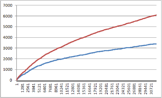
Fig. 1. Numbers of different words (red) and numbers of unique words (blue) in Childe Harold’s Pilgrimage by Byron

2. Empirical analysis

We analyze the number of different words and the number of words encountered once in texts of different authors. These two processes behave like power functions with the same exponent but with different factors.

We estimate the exponent $\theta\in(0,1)$ of the power functions in two different ways. Chebunin and Kovalevskii [16] proposed the estimate

$$\widehat{\theta}=\log_{2}R_{n}-\log_{2}R_{[n/2]}$$

and studied conditions of its consistency and asymptotic normality. It has been used for the analysis of short texts (Zakrevskaya and Kovalevskii [31]).

Another estimate is

$$\theta^{*}=R_{n,1}/R_{n}.$$

Karlin [25] proved that it is consistent for the elementary text model under weak assumptions (see the next section). This is the asymptotically normal estimate under some additional assumptions (Chebunin and Kovalevskii [15]).

For Childe Harold’s Pilgrimage by Byron we have $n=37064$, $R_{n}=6911$, $R_{n/2}=4582$, $\widehat{\theta}=0.5929$, $R_{n,1}=3912$, $\theta^{*}=0.5661$, so the second estimate is significantly smaller than the first one.

Refer to caption
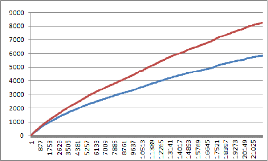
Fig. 2. Numbers of different words (red) and numbers of unique words (blue) in Evgene Onegin by Pushkin

For Evgene Onegin by Pushkin (in Russian) we have $n=21882$, $R_{n}=8236$, $R_{n/2}=4916$, $\widehat{\theta}=0.7445$, $R_{n,1}=5824$, $\theta^{*}=0.7071$, so the second estimate is significantly smaller than the first one.

3. Results for the elementary urn model

The simplest probabilistic model of text is the infinite urn scheme. Words are selected sequentially independently of each other from an infinite dictionary. The probabilities of the appearance of words decrease in accordance with the power distribution according to Zipf’s law. As Bahadur showed, the number of different words is growing according to a power law. Karlin showed that the number of words met once grows under this model also according to a power law with the same exponent.

Karlin [25] studied an infinite urn scheme, that is, $n$ balls distributed to urns independently and randomly; there are infinitely many urns. Each ball goes to urn $i$ with probability $p_{i}>0$, $p_{1}+p_{2}+\ldots=1$ (without loss of generality $p_{1}\geq p_{2}\geq\ldots$).

Let (see Karlin [25]) Ξ ={Π​(t),tβ‰₯0}ΠΠ𝑑𝑑0\Pi=\{\Pi(t),\ t\geq 0\} be a Poisson process with parameter 1. We denote by $X_{i}(n)$ a number of balls in urn $i$. According to well-known property of splitting of Poisson flows, stochastic processes $\{X_{i}(\Pi(t)),\ t\geq 0\}$ are Poisson with intensities $p_{i}$ and are mutually independent for different $i$’s. The definition implies that

RΠ​(t),kβˆ—=βˆ‘i=1βˆžπˆβ€‹(Xi​(Π​(t))β‰₯k),RΠ​(t),k=βˆ‘i=1βˆžπˆβ€‹(Xi​(Π​(t))=k).formulae-sequencesubscriptsuperscriptπ‘…Ξ π‘‘π‘˜superscriptsubscript𝑖1𝐈subscriptπ‘‹π‘–Ξ π‘‘π‘˜subscriptπ‘…Ξ π‘‘π‘˜superscriptsubscript𝑖1𝐈subscriptπ‘‹π‘–Ξ π‘‘π‘˜R^{*}_{\Pi(t),k}=\sum_{i=1}^{\infty}{\bf I}(X_{i}(\Pi(t))\geq k),\ \ R_{\Pi(t),k}=\sum_{i=1}^{\infty}{\bf I}(X_{i}(\Pi(t))=k).

Let designate $\alpha(x)=\max\{j|\ p_{j}\geq 1/x\}$.

We assume, following Karlin [25], that

$$\alpha(x)=x^{\theta}L(x),\ \ 0<\theta<1.$$

Here $L(x)$ is a slowly varying function as $x\to\infty$. Let for $t\in[0,1],\ k\geq 1$

Yn,kβˆ—β€‹(t)=R[n​t],kβˆ—βˆ’π„β€‹R[n​t],kβˆ—(α​(n))1/2,Zn,kβˆ—β€‹(t)=RΠ​(n​t),kβˆ—βˆ’π„β€‹RΠ​(n​t),kβˆ—(α​(n))1/2,formulae-sequencesuperscriptsubscriptπ‘Œπ‘›π‘˜π‘‘subscriptsuperscript𝑅delimited-[]π‘›π‘‘π‘˜π„subscriptsuperscript𝑅delimited-[]π‘›π‘‘π‘˜superscript𝛼𝑛12superscriptsubscriptπ‘π‘›π‘˜π‘‘subscriptsuperscriptπ‘…Ξ π‘›π‘‘π‘˜π„subscriptsuperscriptπ‘…Ξ π‘›π‘‘π‘˜superscript𝛼𝑛12Y_{n,k}^{*}(t)=\frac{R^{*}_{[nt],k}-{\bf E}R^{*}_{[nt],k}}{(\alpha(n))^{1/2}},\ \ \ \ \ \ \ \ \ \ Z_{n,k}^{*}(t)=\frac{R^{*}_{\Pi(nt),k}-{\bf E}R^{*}_{\Pi(nt),k}}{(\alpha(n))^{1/2}},
$$Y_{n,k}(t)=\frac{R_{[nt],k}-{\bf E}R_{[nt],k}}{(\alpha(n))^{1/2}},\ \ \ \ \ \ \ \ \ Z_{n,k}^{**}(t)=\frac{R^{*}_{\Pi([nt]),k}-{\bf E}R^{*}_{\Pi([nt]),k}}{(\alpha(n))^{1/2}},$$

$K_{k,\theta}=\theta\Gamma(k-\theta)$ for $k>0$ and $K_{k,\theta}=-\Gamma(1-\theta)$ for $k=0$.

Proposition 1.

(Theorem 4 in [25]). Let  $\theta\in(0,1]$. Β Then $(R_{n}-{\bf E}R_{n})/B_{n}^{1/2}$ converges weakly to standard normal distribution, where

$$B_{n}=\left\{\begin{array}[]{cr}\Gamma(1-\theta)(2^{\theta}-1)n^{\theta}L(n),&\theta\in(0,1);\\ n\int\limits_{0}^{\infty}\frac{e^{-1/y}}{y}L(ny)dy\stackrel{{\scriptstyle def}}{{=}}nL^{*}(n),&\theta=1;\end{array}\right.$$

Karlin ([25], Lemma 4) proved function $L^{*}(x)$ to be slowly varying as $x\to\infty$.

Dutko [18] generalized the theorem by proving asymptotic normality of $R_{n}$ if ${\bf Var}R_{n}\to\infty$ as $n\to\infty$. This condition always holds if $\theta\in(0,1]$ but can hold too for $\theta=0$. Gnedin, Hansen and Pitman [19] focus on the study of conditions for convergence ${\bf Var}R_{n}\to\infty$. They also collect facts on the issue.

Proposition 2.

(Theorem 5 in [25]). Let $\theta\in(0,1)$, $r_{1}<\ldots<r_{\nu}$ be $\nu$ positive integers. Then random vector $\left(Y_{n,r_{1}}(1),\ldots,Y_{n,r_{\nu}}(1)\right)$ converges weakly to a multivariate normal distribution with zero expectation and covariances

cri,rj={βˆ’ΞΈβ€‹Ξ“β€‹(ri+rjβˆ’ΞΈ)ri!​rj!​2ΞΈβˆ’riβˆ’rj,iβ‰ j;θΓ​(ri+1)​(Γ​(riβˆ’ΞΈ)βˆ’2βˆ’2​ri+θ​Γ​(2​riβˆ’ΞΈ)Γ​(ri+1)),i=j.subscript𝑐subscriptπ‘Ÿπ‘–subscriptπ‘Ÿπ‘—casesπœƒΞ“subscriptπ‘Ÿπ‘–subscriptπ‘Ÿπ‘—πœƒsubscriptπ‘Ÿπ‘–subscriptπ‘Ÿπ‘—superscript2πœƒsubscriptπ‘Ÿπ‘–subscriptπ‘Ÿπ‘—π‘–π‘—πœƒΞ“subscriptπ‘Ÿπ‘–1Ξ“subscriptπ‘Ÿπ‘–πœƒsuperscript22subscriptπ‘Ÿπ‘–πœƒΞ“2subscriptπ‘Ÿπ‘–πœƒΞ“subscriptπ‘Ÿπ‘–1𝑖𝑗c_{r_{i},r_{j}}=\left\{\begin{array}[]{cr}-\frac{\theta\Gamma(r_{i}+r_{j}-\theta)}{r_{i}!r_{j}!}2^{\theta-r_{i}-r_{j}},&i\neq j;\\ \frac{\theta}{\Gamma(r_{i}+1)}\left(\Gamma(r_{i}-\theta)-2^{-2r_{i}+\theta}\frac{\Gamma(2r_{i}-\theta)}{\Gamma(r_{i}+1)}\right),&i=j.\end{array}\right.

Barbour and Gnedin [8] extended this result to the case $\theta=0$ if variances go to infinity. They found conditions for convergence of covariances to a limit and identified four types of limiting behavior of variances. Barbour [7] proved theorems on the approximation of the number of cells with $k$ balls by translated Poisson distribution. Key [26], [27] studied the limit behavior of statistics $R_{n,1}$. Hwang and Janson [23] proved local limit theorems for finite and infinite numbers of cells. Chebunin [13] constructed $R_{n}$-based explicit parameter estimators for a wide range of one-parameter families and proved their consistency.

Durieu and Wang [17] established a functional central limit theorem for randomization of a process $R_{n}$: indicators are multiplied randomly by $\pm 1$ before summing. The limiting Gaussian process is a sum of independent self-similar processes in this case.

Chebunin $\&$ Kovalevskii [14] proved the next FCLT.

Proposition 3.

(i) Let $\theta\in(0,1)$, $\nu\geq 1$ is integer. Then process $\left(Y^{*}_{n,1}(t),\ldots,Y^{*}_{n,\nu}(t),\ 0\leq t\leq 1\right)$ converges weakly in the uniform metrics in $D(0,1)$ to $\nu$-dimensional Gaussian process with zero expectation and covariance function $(c^{*}_{ij}(\tau,t))_{i,j=1}^{\nu}$: for $\tau\leq t$, $i,j\in\{1,\ldots,\nu\}$ (taking $0^{0}=1$)

ci​jβˆ—β€‹(Ο„,t)={βˆ‘s=0iβˆ’1βˆ‘m=0jβˆ’sβˆ’1Ο„s​(tβˆ’Ο„)m​Km+s,ΞΈtm+sβˆ’ΞΈβ€‹s!​m!βˆ’βˆ‘s=0iβˆ’1βˆ‘m=0jβˆ’1Ο„s​tm​Km+s,ΞΈ(t+Ο„)m+sβˆ’ΞΈβ€‹s!​m!,i<j;tΞΈβ€‹βˆ‘m=0jβˆ’1Km,ΞΈm!βˆ’βˆ‘s=0iβˆ’1βˆ‘m=0jβˆ’1Ο„s​tm​Km+s,ΞΈ(t+Ο„)m+sβˆ’ΞΈβ€‹s!​m!,iβ‰₯j;subscriptsuperscriptπ‘π‘–π‘—πœπ‘‘casessuperscriptsubscript𝑠0𝑖1superscriptsubscriptπ‘š0𝑗𝑠1superscriptπœπ‘ superscriptπ‘‘πœπ‘šsubscriptπΎπ‘šπ‘ πœƒsuperscriptπ‘‘π‘šπ‘ πœƒπ‘ π‘šsuperscriptsubscript𝑠0𝑖1superscriptsubscriptπ‘š0𝑗1superscriptπœπ‘ superscriptπ‘‘π‘šsubscriptπΎπ‘šπ‘ πœƒsuperscriptπ‘‘πœπ‘šπ‘ πœƒπ‘ π‘šπ‘–π‘—superscriptπ‘‘πœƒsuperscriptsubscriptπ‘š0𝑗1subscriptπΎπ‘šπœƒπ‘šsuperscriptsubscript𝑠0𝑖1superscriptsubscriptπ‘š0𝑗1superscriptπœπ‘ superscriptπ‘‘π‘šsubscriptπΎπ‘šπ‘ πœƒsuperscriptπ‘‘πœπ‘šπ‘ πœƒπ‘ π‘šπ‘–π‘—c^{*}_{ij}(\tau,t)=\left\{\begin{array}[]{cr}\sum\limits_{s=0}^{i-1}\sum\limits_{m=0}^{j-s-1}\frac{\tau^{s}(t-\tau)^{m}K_{m+s,\theta}}{t^{m+s-\theta}s!m!}-\sum\limits_{s=0}^{i-1}\sum\limits_{m=0}^{j-1}\frac{\tau^{s}t^{m}K_{m+s,\theta}}{(t+\tau)^{m+s-\theta}s!m!},&i<j;\\ t^{\theta}\sum\limits_{m=0}^{j-1}\frac{K_{m,\theta}}{m!}-\sum\limits_{s=0}^{i-1}\sum\limits_{m=0}^{j-1}\frac{\tau^{s}t^{m}K_{m+s,\theta}}{(t+\tau)^{m+s-\theta}s!m!},&i\geq j;\\ \end{array}\right.

$c^{*}_{ij}(\tau,t)=c^{*}_{ji}(t,\tau)$.

(ii) Let $\theta=1$. Then process $\left(\frac{R_{[nt]}-{\bf E}R_{[nt]}}{(nL^{*}(n))^{1/2}},\ 0\leq t\leq 1\right)$ converges weakly in the uniform metrics in $D(0,1)$ to a standard Wiener process.

4. Results for Simon model

Yule showed that, for the Yuleβ€”Simon model,

(1) $${\bf E}R_{n,i}/{\bf E}R_{n}\to f(i),\ \ i\geq 1,$$
$$f(i)=\rho B(i,1+\rho),$$

$\rho=(1-p)^{-1}$, $B(\cdot,\cdot)$ is Beta function.

We analyze stochastic aspects of this convergence. The limiting distribution is named Yule-Simon distribution.

There are many ramifications and applications of the Yule-Simon model. Haight $\&$ Jones [20] gave special references to word associations tests. Lansky $\&$ Radill-Weiss [28] proposed a generalization of the model for better correspondence to applications.

This model can be embedded in a more general context of random cutting of recursive trees. In this context, statistics under study are the most frequent words. See Aldous $\&$ Pitman [5] for its limiting distribution and convergence, Baur $\&$ Bertoin [9], [10] for an overview and new results.

Aldous [4] proposed a generalization of the limiting distribution but without an underlying process.

Janson [24] considered generalized Polya urns and proved SLLN, CLT and FCLT for it. Finite-dimensional vectors

$$(R_{n},R_{n,1},\ldots,R_{n,m-1},n-\sum_{i<m}iR_{n,i})$$

can be studied using these models. So we have componentwise SLLN and finite-dimensional CLT and FCLT for these statistics.

Theorem 1.

For any $p\in(0,1)$ in Simon model and any $m>1$

$$\frac{R_{n}}{n}\to p\ \ {\rm a.s.},$$
$$\frac{(R_{n,1},\ldots,R_{n,m-1})}{n}\to\frac{p}{1-p}\left(B\left(1,\frac{2-p}{1-p}\right),\ldots B\left(m-1,\frac{2-p}{1-p}\right)\right)\ \ {\rm a.s.},$$

and, in $D[0,\infty)$,

$$\left\{n^{-1/2}(R_{[nt]}-tnp),\right.$$
$$\left.n^{-1/2}\left(R_{[nt],j}-tn\frac{p}{1-p}B\left(j,\frac{2-p}{1-p}\right)\right),\ 1\leq j\leq m-1,\ t\geq 0\right\}\to_{d}V(t),$$

where $V(t)$ is a continuous centered $m$-dimensional Gaussian process, its covariance matrix-function ${\bf E}V(x)V^{T}(y)$ depends on $p,x,y$ only.

Proof

Simon’s model can be studied as a very partial case of Janson’s [24] urn scheme. In this model, Simon urns with $1\leq i\leq m-1$ balls are balls with numbers from 2 to $m$ with weights $a_{i}=i-1$. The $(m+1)$-th urn contains all other balls with weights $a_{m+1}=1$. Balls with number 1 correspond to all different words, $a_{1}=0$. So the random uniform choice of balls in the Simon model corresponds to the random choice with weights $a_{i}$, $1\leq i\leq m+1$, in Janson model.

Let $({\bf e}_{1},\ldots,{\bf e}_{m+1})$ be the standard basis in ${\bf R}^{m}$, then increment vectors in Janson model are

$$\xi_{i}={\bf e}_{1}+{\bf e}_{2}\ {\rm with\ probability}\ p,\ \ \xi_{i}={\bf e}_{i+1}-{\bf e}_{i}\ {\rm with\ probability}\ q=1-p,\ \ 2\leq i<m,$$
$$\xi_{m}={\bf e}_{1}+{\bf e}_{2}\ {\rm with\ probability}\ p,\ \ \xi_{m}=m{\bf e}_{m+1}-{\bf e}_{m}\ {\rm with\ probability}\ q=1-p,$$
$$\xi_{m+1}={\bf e}_{1}+{\bf e}_{2}\ {\rm with\ probability}\ p,\ \ \xi_{m+1}={\bf e}_{m+1}\ {\rm with\ probability}\ q=1-p.$$

So matrix $A=(a_{j}{\bf E}\xi_{ji})$ has the first (maximal) eigenvalue $\lambda_{1}=1$, the next (second) eigenvalue $\lambda_{2}=0$. Thus the assumption $\lambda_{2}<\lambda_{1}/2$ of Theorem 2.22 and Theorem 2.31(i) in Janson [24] is hold. So we use Janson’s theorems 2.21 (SLLN), 2.22, 2.31(i).

The proof is complete.

5. Offline Simon modification of the Karlin model

Let the balls take urns as in the Karlin model, but the appearance of a new non-empty urn corresponds only to the embryo of a new word.

After the finish of the Karlin model, Simon’s model starts to work in moments of the appearance of the embryos of new words: the $k$-th embryo coincides with each of the previous embryos with probability $q/k$, and is a new word with probability $p$, $p+q=1$. We use Janson’s theorems.

Balls of the first type are embryos of words encountered exactly once, their number at the $k$ -th step is $X_{k,1}$, balls of this type have weights (responsible for the probabilities of choosing balls) $a_{1}=1$.

Balls of the second type are embryos of words encountered more than once, their number at the $k$ -th step is $X_{k,2}$, balls of this type have weights $a_{2}=1$ also.

The system starts from the state $X_{0,1}=1,X_{0,2}=0$. At each step $k$, one ball is chosen at random from $X_{k,1}+X_{k,2}$ balls of the first and second types.

If the selected ball is of the first type, then a ball of the first type is added with probability $p$, and it is replaced by a ball of the second type with probabilityΒ qπ‘žq:

$$X_{0}=(1,0)^{\prime},$$
$$\xi_{1}=(1,0)^{\prime}\ \text{with probability}\ p,$$
$$\xi_{1}=(-1,1)^{\prime}\ \text{with probability}\ q.$$

If the chosen ball is of the second type, then a ball of the first type is added with probability $p$, and nothing happens with probability $q$:

$$\xi_{2}=(1,0)^{\prime}\ \text{with probability}\ p,$$
$$\xi_{2}=(0,0)^{\prime}\ \text{with probability}\ q.$$

So

$$A=\left(a_{j}{\bf E}\xi_{ji}\right)_{i,j=1}^{2}=\left(\begin{array}[]{cc}p-q&p\\ q&0\end{array}\right).$$

Eigenvalues of $A$ are $\lambda_{1}=p$, $\lambda_{2}=-q<\lambda_{1}/2$.

Eigenvector $v_{1}$ of $A$ correspond to eigenvalue $\lambda_{1}=p$ and condition (2.2) from Janson [24] $a\cdot v_{1}=1$. As $a=(1\,1)^{\prime}$, we have

$$v_{1}=\left(\begin{array}[]{c}p\\ q\end{array}\right).$$

We calculate $e^{tA}$ using Sylvester’s formula:

$$e^{tA}=\frac{e^{pt}}{p+q}(A+qI)-\frac{e^{-qt}}{p+q}(A-pI)=e^{pt}(A+qI)-e^{-qt}(A-pI).$$

From (3.17) in Janson [24],

ϕ​(s,A)=∫0set​A​𝑑t=ep​sβˆ’1p​(A+q​I)+eβˆ’q​sβˆ’1q​(Aβˆ’p​I)italic-ϕ𝑠𝐴superscriptsubscript0𝑠superscript𝑒𝑑𝐴differential-d𝑑superscript𝑒𝑝𝑠1π‘π΄π‘žπΌsuperscriptπ‘’π‘žπ‘ 1π‘žπ΄π‘πΌ\phi(s,A)=\int_{0}^{s}e^{tA}dt=\frac{e^{ps}-1}{p}(A+qI)+\frac{e^{-qs}-1}{q}(A-pI)

From (3.18) in [24],

Οˆβ€‹(s,A)=es​Aβˆ’Ξ»1​v1​a′​ϕ​(s,A)πœ“π‘ π΄superscript𝑒𝑠𝐴subscriptπœ†1subscript𝑣1superscriptπ‘Žβ€²italic-ϕ𝑠𝐴\psi(s,A)=e^{sA}-\lambda_{1}v_{1}a^{\prime}\phi(s,A)
=ep​s​(A+q​I)βˆ’eβˆ’q​s​(Aβˆ’p​I)βˆ’p​v1​a′​(ep​sβˆ’1p​(A+q​I)+eβˆ’q​sβˆ’1q​(Aβˆ’p​I)).absentsuperscriptπ‘’π‘π‘ π΄π‘žπΌsuperscriptπ‘’π‘žπ‘ π΄π‘πΌπ‘subscript𝑣1superscriptπ‘Žβ€²superscript𝑒𝑝𝑠1π‘π΄π‘žπΌsuperscriptπ‘’π‘žπ‘ 1π‘žπ΄π‘πΌ=e^{ps}(A+qI)-e^{-qs}(A-pI)-pv_{1}a^{\prime}\left(\frac{e^{ps}-1}{p}(A+qI)+\frac{e^{-qs}-1}{q}(A-pI)\right).

Note that

$$v_{1}a^{\prime}=A+qI=(A+qI)^{2}.$$

So

Οˆβ€‹(s,A)=βˆ’eβˆ’q​s​(Aβˆ’p​I)+A+q​Iβˆ’p​(eβˆ’q​sβˆ’1)q​(A+q​I)​(Aβˆ’p​I).πœ“π‘ π΄superscriptπ‘’π‘žπ‘ π΄π‘πΌπ΄π‘žπΌπ‘superscriptπ‘’π‘žπ‘ 1π‘žπ΄π‘žπΌπ΄π‘πΌ\psi(s,A)=-e^{-qs}(A-pI)+A+qI-\frac{p(e^{-qs}-1)}{q}(A+qI)(A-pI).
=A+q​Iβˆ’eβˆ’q​s​(Aβˆ’p​I).absentπ΄π‘žπΌsuperscriptπ‘’π‘žπ‘ π΄π‘πΌ=A+qI-e^{-qs}(A-pI).

Let

$$A_{0}:=A+qI,$$

then

Οˆβ€‹(s,A)=A0​(1βˆ’eβˆ’q​s)+I​eβˆ’q​s.πœ“π‘ π΄subscript𝐴01superscriptπ‘’π‘žπ‘ πΌsuperscriptπ‘’π‘žπ‘ \psi(s,A)=A_{0}(1-e^{-qs})+Ie^{-qs}.

We calculate matrices $B_{1}$, $B_{2}$, $B$. From (2.13) in [24],

$$B_{1}={\bf E}\xi_{1}\xi_{1}^{\prime}=p\left(\begin{array}[]{cc}1&0\\ 0&0\end{array}\right)+q\left(\begin{array}[]{cc}1&-1\\ -1&1\end{array}\right)=\left(\begin{array}[]{cc}1&-q\\ -q&q\end{array}\right),$$
$$B_{2}={\bf E}\xi_{2}\xi_{2}^{\prime}=\left(\begin{array}[]{cc}p&0\\ 0&0\end{array}\right).$$

From (2.14) in [24],

$$B=a_{1}v_{11}B_{1}+a_{2}v_{12}B_{2}=p\left(\begin{array}[]{cc}1+q&-q\\ -q&q\end{array}\right).$$

From Theorem 3.21 in [24],

Xnnβ†’a.s.Ξ»1​v1=p​v1.subscriptβ†’formulae-sequenceπ‘Žπ‘ subscript𝑋𝑛𝑛subscriptπœ†1subscript𝑣1𝑝subscript𝑣1\frac{X_{n}}{n}\to_{a.s.}\lambda_{1}v_{1}=pv_{1}.

From Theorem 3.22 in [24],

$$\frac{X_{n}-n\lambda_{1}v_{1}}{\sqrt{n}}\to_{d}N(0,\Sigma),$$
Ξ£=∫0βˆžΟˆβ€‹(s,A)​Bβ€‹Οˆβ€‹(s,A)′​eβˆ’Ξ»1​s​λ1​𝑑sβˆ’Ξ»12​v1​v1β€²Ξ£superscriptsubscript0πœ“π‘ π΄π΅πœ“superscript𝑠𝐴′superscript𝑒subscriptπœ†1𝑠subscriptπœ†1differential-d𝑠superscriptsubscriptπœ†12subscript𝑣1superscriptsubscript𝑣1β€²\Sigma=\int_{0}^{\infty}\psi(s,A)B\psi(s,A)^{\prime}e^{-\lambda_{1}s}\lambda_{1}ds-\lambda_{1}^{2}v_{1}v_{1}^{\prime}
=∫0∞(A0​(1βˆ’eβˆ’q​s)+I​eβˆ’q​s)​B​(A0′​(1βˆ’eβˆ’q​s)+I​eβˆ’q​s)​eβˆ’p​s​p​𝑑sabsentsuperscriptsubscript0subscript𝐴01superscriptπ‘’π‘žπ‘ πΌsuperscriptπ‘’π‘žπ‘ π΅superscriptsubscript𝐴0β€²1superscriptπ‘’π‘žπ‘ πΌsuperscriptπ‘’π‘žπ‘ superscript𝑒𝑝𝑠𝑝differential-d𝑠=\int_{0}^{\infty}\left(A_{0}(1-e^{-qs})+Ie^{-qs}\right)B\left(A_{0}^{\prime}(1-e^{-qs})+Ie^{-qs}\right)e^{-ps}pds
$$-p^{2}\left(\begin{array}[]{cc}p^{2}&pq\\ pq&q^{2}\end{array}\right)$$
=∫0∞(A0​B​A0β€²+eβˆ’q​s​(A0​B+B​A0β€²βˆ’2​A0​B​A0β€²)+eβˆ’2​q​s​(B+A0​B​A0β€²))​eβˆ’p​s​p​𝑑sabsentsuperscriptsubscript0subscript𝐴0𝐡superscriptsubscript𝐴0β€²superscriptπ‘’π‘žπ‘ subscript𝐴0𝐡𝐡superscriptsubscript𝐴0β€²2subscript𝐴0𝐡superscriptsubscript𝐴0β€²superscript𝑒2π‘žπ‘ π΅subscript𝐴0𝐡superscriptsubscript𝐴0β€²superscript𝑒𝑝𝑠𝑝differential-d𝑠=\int_{0}^{\infty}\left(A_{0}BA_{0}^{\prime}+e^{-qs}(A_{0}B+BA_{0}^{\prime}-2A_{0}BA_{0}^{\prime})+e^{-2qs}(B+A_{0}BA_{0}^{\prime})\right)e^{-ps}pds
$$-p^{2}\left(\begin{array}[]{cc}p^{2}&pq\\ pq&q^{2}\end{array}\right)$$
$$=A_{0}BA_{0}^{\prime}+p(A_{0}B+BA_{0}^{\prime}-2A_{0}BA_{0}^{\prime})+\frac{p}{1+q}(B+A_{0}BA_{0}^{\prime})-p^{2}\left(\begin{array}[]{cc}p^{2}&pq\\ pq&q^{2}\end{array}\right)$$
$$=pq\left(\begin{array}[]{cc}3p^{2}+p&p-3p^{2}\\ p-3p^{2}&1-3p+3p^{2}\end{array}\right).$$

From Theorem 3.31 in [24], there is FCLT for $\{X_{[nt]},\ 0\leq t\leq 1\}$:

$$\left\{\frac{X_{[nt]}-nt\lambda_{1}v_{1}}{\sqrt{n}},\ 0\leq t\leq 1\right\}\to_{d}U=\{U(t),\ 0\leq t\leq 1\}$$

in the uniform metrics, $U$ is the centered Gaussian process, and for $0<x\leq y$

𝐄​U​(x)​U′​(y)=βˆ«βˆ’Ξ»1βˆ’1​log⁑xβˆžΟˆβ€‹(s+Ξ»1βˆ’1​log⁑x,A)​Bβ€‹Οˆβ€‹(s+Ξ»1βˆ’1​log⁑y,A)′​eβˆ’Ξ»1​x​λ1​𝑑xβˆ’x​λ12​v1​v1β€²π„π‘ˆπ‘₯superscriptπ‘ˆβ€²π‘¦superscriptsubscriptsuperscriptsubscriptπœ†11π‘₯πœ“π‘ superscriptsubscriptπœ†11π‘₯π΄π΅πœ“superscript𝑠superscriptsubscriptπœ†11𝑦𝐴′superscript𝑒subscriptπœ†1π‘₯subscriptπœ†1differential-dπ‘₯π‘₯superscriptsubscriptπœ†12subscript𝑣1superscriptsubscript𝑣1β€²{\bf E}U(x)U^{\prime}(y)=\int\limits_{-\lambda_{1}^{-1}\log x}^{\infty}\psi(s+\lambda_{1}^{-1}\log x,A)B\psi(s+\lambda_{1}^{-1}\log y,A)^{\prime}e^{-\lambda_{1}x}\lambda_{1}dx-x\lambda_{1}^{2}v_{1}v_{1}^{\prime}
=βˆ«βˆ’Ξ»1βˆ’1​log⁑x∞(A0​(1βˆ’eβˆ’q​(s+log⁑x/p))+I​eβˆ’q​(s+log⁑x/p))​Babsentsuperscriptsubscriptsuperscriptsubscriptπœ†11π‘₯subscript𝐴01superscriptπ‘’π‘žπ‘ π‘₯𝑝𝐼superscriptπ‘’π‘žπ‘ π‘₯𝑝𝐡=\int\limits_{-\lambda_{1}^{-1}\log x}^{\infty}\left(A_{0}(1-e^{-q(s+\log x/p)})+Ie^{-q(s+\log x/p)}\right)B
Γ—(A0′​(1βˆ’eβˆ’q​(s+log⁑y/p))+I​eβˆ’q​(s+log⁑y/p))​eβˆ’Ξ»1​x​λ1​d​xβˆ’x​λ12​v1​v1β€²absentsuperscriptsubscript𝐴0β€²1superscriptπ‘’π‘žπ‘ π‘¦π‘πΌsuperscriptπ‘’π‘žπ‘ π‘¦π‘superscript𝑒subscriptπœ†1π‘₯subscriptπœ†1𝑑π‘₯π‘₯superscriptsubscriptπœ†12subscript𝑣1superscriptsubscript𝑣1β€²\times\left(A_{0}^{\prime}(1-e^{-q(s+\log y/p)})+Ie^{-q(s+\log y/p)}\right)e^{-\lambda_{1}x}\lambda_{1}dx-x\lambda_{1}^{2}v_{1}v_{1}^{\prime}
$$=xpq\left(\begin{array}[]{cc}2p^{2}&2pq\\ pq-p^{2}&q^{2}-pq\end{array}\right)+xp^{2}q\left(\frac{x}{y}\right)^{q/p}\left(\begin{array}[]{cc}1+p&-1-p\\ -p&p\end{array}\right).$$

We have a good match for Childe Harold’s Pilgrimage with $\theta=0.58$, $p=0.56$, for Evgene Onegin with $\theta=0.74$, $p=0.71$.

6. Compound Poisson modification of the Karlin model

We want to invent a text model such that $\theta^{*}$ converges to a number less than $\widehat{\theta}$. We propose the following simple model: words appear in the same way as in Karlin’s model, but each word with probability $q_{i}$ (independently of others and of the process of the appearance of words) is repeated $i\geq 1$ times, $q_{1}+q_{2}+\ldots=1$. New statistics of the number of different words and the number of words that occur once are denoted by $\mathbb{R}_{n}$ and $\mathbb{R}_{n,1}$.

The Poisson version of these processes uses the compound Poisson process.

We want to invent a text model such that $\theta^{*}$ converges to a number less than $\widehat{\theta}$. We propose the following simple model: words appear in the same way as in Karlin’s model, but each word with probability $q_{i}$ (independently of others and of the process of the appearance of words) is repeated $i\geq 1$ times, $q_{1}+q_{2}+\ldots=1$. New statistics of the number of different words and the number of words that occur once are denoted by ${\mathbb{R}}_{n}$ and ${\mathbb{R}}_{n,1}$. We denote by ${\mathbb{X}}_{i}(n)$ a number of balls in urn $i$, and

$$\mathbb{R}_{n,k}^{*}=\sum_{i=1}^{\infty}\mathbf{I}\left(\mathbb{X}_{i}(n)\geq k\right),\ \ \mathbb{R}_{n}=\mathbb{R}_{n,1}^{*},\ \ \mathbb{R}_{n,k}=\mathbb{R}_{n,k}^{*}-\mathbb{R}_{n,k+1}^{*}.$$

The Poisson version of these processes uses the compound Poisson process. Let Ξ ={Π​(t),tβ‰₯0}ΠΠ𝑑𝑑0\Pi=\{\Pi(t),t\geq 0\} be a Poisson process with parameter $1$. The Poissonized version of Karlin model assumes the total number of $\Pi(n)$ balls. According to well-known thinning property of Poisson flows, stochastic processes $\left\{{\mathbb{X}}_{i}(\Pi(t))\stackrel{{\scriptstyle\text{ def }}}{{=}}\mathbf{\Pi}_{i}(t),t\geq 0\right\}$ are compound Poisson with intensities $p_{i}$ and are mutually independent for different $i$ ’s. The definition implies that

ℝΠ​(n),kβˆ—=βˆ‘i=1βˆžπˆβ€‹(𝚷i​(n)β‰₯k),ℝΠ​(n),k=βˆ‘i=1βˆžπˆβ€‹(𝚷i​(n)=k).formulae-sequencesuperscriptsubscriptβ„Ξ π‘›π‘˜superscriptsubscript𝑖1𝐈subscriptπš·π‘–π‘›π‘˜subscriptβ„Ξ π‘›π‘˜superscriptsubscript𝑖1𝐈subscriptπš·π‘–π‘›π‘˜\mathbb{R}_{\Pi(n),k}^{*}=\sum_{i=1}^{\infty}\mathbf{I}\left(\mathbf{\Pi}_{i}(n)\geq k\right),\quad\mathbb{R}_{\Pi(n),k}=\sum_{i=1}^{\infty}\mathbf{I}\left(\mathbf{\Pi}_{i}(n)=k\right).

We proved FCLT for the vector process $({\mathbb{R}}_{n},\ {\mathbb{R}}_{n,1})$. Let $\alpha(x)=\max\left\{j\mid p_{j}\geq 1/x\right\}.$ Following Karlin [25], we assume that $\alpha(x)=x^{\theta}L(x),0\leq\theta\leq 1$. Here $L(x)$ is a slowly varying function as $x\rightarrow\infty$. Let for $t\in[0,1],k\geq 1$

𝕐n,kβˆ—β€‹(t)=ℝ[n​t],kβˆ—βˆ’π„β€‹β„[n​t],kβˆ—(α​(n))1/2,β„€n,kβˆ—β€‹(t)=ℝΠ​(n​t),kβˆ—βˆ’π„β€‹β„Ξ β€‹(n​t),kβˆ—(α​(n))1/2,formulae-sequencesuperscriptsubscriptπ•π‘›π‘˜π‘‘superscriptsubscriptℝdelimited-[]π‘›π‘‘π‘˜π„superscriptsubscriptℝdelimited-[]π‘›π‘‘π‘˜superscript𝛼𝑛12superscriptsubscriptβ„€π‘›π‘˜π‘‘superscriptsubscriptβ„Ξ π‘›π‘‘π‘˜π„superscriptsubscriptβ„Ξ π‘›π‘‘π‘˜superscript𝛼𝑛12\mathbb{Y}_{n,k}^{*}(t)=\frac{\mathbb{R}_{[nt],k}^{*}-\mathbf{E}\mathbb{R}_{[nt],k}^{*}}{(\alpha(n))^{1/2}},\ \ \mathbb{Z}_{n,k}^{*}(t)=\frac{\mathbb{R}_{\Pi(nt),k}^{*}-\mathbf{E}\mathbb{R}_{\Pi(nt),k}^{*}}{(\alpha(n))^{1/2}},
$$\ \ \mathbb{Y}_{n,k}(t)=\frac{\mathbb{R}_{[nt],k}-\mathbf{E}\mathbb{R}_{[nt],k}}{(\alpha(n))^{1/2}}.$$
Theorem 2.

Let $\theta\in(0,1)$ and $v\geq 1$ be an integer. Then process $\left(\mathbb{Y}_{n,1}^{*}(t),\ldots,\mathbb{Y}_{n,v}^{*}(t),0\leq t\leq 1\right)$ converges weakly in the uniform metric in $D\left([0,1]^{v}\right)$ to $v$ -dimensional Gaussian process with zero expectation and covariance function $\left(\mathbb{C}_{ij}^{*}(\tau,t)\right)_{i,j=1}^{v}$.

Lemma 1.

(i) There exist $n_{0}\geq 1$, $C(\theta)<\infty$ such that 𝐄​RΠ​(n​δ)/α​(n)≀C​(ΞΈ)​δθ/2𝐄subscriptπ‘…Ξ π‘›π›Ώπ›Όπ‘›πΆπœƒsuperscriptπ›Ώπœƒ2{\bf E}R_{\Pi(n\delta)}/\alpha(n)\leq C(\theta)\delta^{\theta/2} for any $\delta\in[0,1],\ n\geq n_{0}$.

(ii) Let $\tau\leq t$, then 𝐄​(ℝΠ​(t),kβˆ—βˆ’β„Ξ β€‹(Ο„),kβˆ—)≀𝐄​RΠ​(tβˆ’Ο„)𝐄subscriptsuperscriptβ„Ξ π‘‘π‘˜subscriptsuperscriptβ„Ξ πœπ‘˜π„subscriptπ‘…Ξ π‘‘πœ{\bf E}(\mathbb{R}^{*}_{\Pi(t),k}-\mathbb{R}^{*}_{\Pi(\tau),k})\leq{\bf E}R_{\Pi(t-\tau)}, $k\geq 1$.

(iii) For any pair $\varepsilon$, $\delta\in(0,1)$ there exists integer $n_{0}$ such that 𝐏(βˆ€t∈[0,1]βˆƒΟ„:|Ο„βˆ’t|≀δ,Ξ (nΟ„)=[nt])=d​e​f𝐏(A(n))β‰₯1βˆ’Ξ΅/2{\bf P}(\forall t\in[0,1]\ \ \exists\tau:|\tau-t|\leq\delta,\ \Pi(n\tau)=[nt])\stackrel{{\scriptstyle def}}{{=}}{\bf P}(A(n))\geq 1-\varepsilon/2 for any $n\geq n_{0}$.

Proof. (i) and (iii) were proved in Chebunin and Kovalevskii [16], (ii) follows from

𝐄​(ℝΠ​(t),kβˆ—βˆ’β„Ξ β€‹(Ο„),kβˆ—)=βˆ‘i=1βˆžβˆ‘j=0kβˆ’1𝐏​(𝚷i​(Ο„)=j)​𝐏​(𝚷i​(t)βˆ’πš·i​(Ο„)β‰₯kβˆ’j)𝐄superscriptsubscriptβ„Ξ π‘‘π‘˜superscriptsubscriptβ„Ξ πœπ‘˜superscriptsubscript𝑖1superscriptsubscript𝑗0π‘˜1𝐏subscriptπš·π‘–πœπ‘—πsubscriptπš·π‘–π‘‘subscriptπš·π‘–πœπ‘˜π‘—\mathbf{E}\left(\mathbb{R}_{\Pi(t),k}^{*}-\mathbb{R}_{\Pi(\tau),k}^{*}\right)=\sum_{i=1}^{\infty}\sum_{j=0}^{k-1}\mathbf{P}\left(\mathbf{\Pi}_{i}(\tau)=j\right)\mathbf{P}\left(\mathbf{\Pi}_{i}(t)-\mathbf{\Pi}_{i}(\tau)\geq k-j\right)
β‰€βˆ‘i=1βˆžπβ€‹(𝚷i​(tβˆ’Ο„)β‰₯1)=𝐄​ℝΠ​(tβˆ’Ο„)=𝐄​RΠ​(tβˆ’Ο„).absentsuperscriptsubscript𝑖1𝐏subscriptπš·π‘–π‘‘πœ1𝐄subscriptβ„Ξ π‘‘πœπ„subscriptπ‘…Ξ π‘‘πœ\leq\sum_{i=1}^{\infty}\mathbf{P}\left(\mathbf{\Pi}_{i}(t-\tau)\geq 1\right)=\mathbf{E}\mathbb{R}_{\Pi(t-\tau)}=\mathbf{E}R_{\Pi(t-\tau)}.

The proof is complete.

Proof of TheoremΒ 2

Step 1 (covariances) Let $\tau\leq t$, $i\leq j$ and $\pi_{k,i}(t)=\mathbf{P}(\mathbf{\Pi}_{k}(t)=i)$

πœπ¨π―β€‹(ℝΠ​(Ο„),iβˆ—,ℝΠ​(t),jβˆ—)=βˆ‘k=1∞(𝐏​(𝚷k​(Ο„)<i,𝚷k​(t)<j)βˆ’πβ€‹(𝚷k​(Ο„)<i)​𝐏​(𝚷k​(t)<j))𝐜𝐨𝐯superscriptsubscriptβ„Ξ πœπ‘–superscriptsubscriptℝΠ𝑑𝑗superscriptsubscriptπ‘˜1𝐏formulae-sequencesubscriptπš·π‘˜πœπ‘–subscriptπš·π‘˜π‘‘π‘—πsubscriptπš·π‘˜πœπ‘–πsubscriptπš·π‘˜π‘‘π‘—{\bf cov}\left(\mathbb{R}_{\Pi(\tau),i}^{*},\mathbb{R}_{\Pi(t),j}^{*}\right)=\sum_{k=1}^{\infty}\left(\mathbf{P}\left(\mathbf{\Pi}_{k}(\tau)<i,\mathbf{\Pi}_{k}(t)<j\right)-\mathbf{P}\left(\mathbf{\Pi}_{k}(\tau)<i\right)\mathbf{P}\left(\mathbf{\Pi}_{k}(t)<j\right)\right)
=βˆ‘k=1βˆžβˆ‘s=0iβˆ’1Ο€k,s​(Ο„)​(βˆ‘m=0jβˆ’sβˆ’1Ο€k,m​(tβˆ’Ο„)βˆ’βˆ‘m=0jβˆ’1Ο€k,m​(t)),absentsuperscriptsubscriptπ‘˜1superscriptsubscript𝑠0𝑖1subscriptπœ‹π‘˜π‘ πœsuperscriptsubscriptπ‘š0𝑗𝑠1subscriptπœ‹π‘˜π‘šπ‘‘πœsuperscriptsubscriptπ‘š0𝑗1subscriptπœ‹π‘˜π‘šπ‘‘=\sum_{k=1}^{\infty}\sum_{s=0}^{i-1}\pi_{k,s}(\tau)\left(\sum_{m=0}^{j-s-1}\pi_{k,m}(t-\tau)-\sum_{m=0}^{j-1}\pi_{k,m}(t)\right),

and $i>j$

πœπ¨π―β€‹(ℝΠ​(Ο„),iβˆ—,ℝΠ​(t),jβˆ—)=βˆ‘k=1βˆžβˆ‘s=0jβˆ’1Ο€k,s​(t)​(1βˆ’βˆ‘m=0iβˆ’1Ο€k,m​(Ο„)).𝐜𝐨𝐯superscriptsubscriptβ„Ξ πœπ‘–superscriptsubscriptℝΠ𝑑𝑗superscriptsubscriptπ‘˜1superscriptsubscript𝑠0𝑗1subscriptπœ‹π‘˜π‘ π‘‘1superscriptsubscriptπ‘š0𝑖1subscriptπœ‹π‘˜π‘šπœ{\bf cov}\left(\mathbb{R}_{\Pi(\tau),i}^{*},\mathbb{R}_{\Pi(t),j}^{*}\right)=\sum_{k=1}^{\infty}\sum_{s=0}^{j-1}\pi_{k,s}(t)\left(1-\sum_{m=0}^{i-1}\pi_{k,m}(\tau)\right).

Let $t^{\prime}=t(1-q_{0})$, $c_{1}=q_{1}/(1-q_{0})$

$$\mathbf{E}\mathbb{R}_{\Pi(t)}=\sum_{k=1}^{\infty}1-\pi_{k,0}(t)=\sum_{k=1}^{\infty}1-e^{-p_{k}t}=\mathbf{E}R_{\Pi(t)},\ \ \mathbf{D}\mathbb{R}_{\Pi(t)}=\mathbf{D}R_{\Pi(t)}.$$
𝐄​ℝΠ​(t),1=βˆ‘k=1βˆžΟ€k,1​(t)=βˆ‘k=1∞q1​𝐏​(Ξ k​(t)=1)=q1​𝐄​RΠ​(t),1.𝐄subscriptℝΠ𝑑1superscriptsubscriptπ‘˜1subscriptπœ‹π‘˜1𝑑superscriptsubscriptπ‘˜1subscriptπ‘ž1𝐏subscriptΞ π‘˜π‘‘1subscriptπ‘ž1𝐄subscript𝑅Π𝑑1\mathbf{E}\mathbb{R}_{\Pi(t),1}=\sum_{k=1}^{\infty}\pi_{k,1}(t)=\sum_{k=1}^{\infty}q_{1}\mathbf{P}(\Pi_{k}(t)=1)=q_{1}\mathbf{E}R_{\Pi(t),1}.
πœπ¨π―β€‹(ℝΠ​(Ο„)βˆ—,ℝΠ​(t)βˆ—)=βˆ‘k=1βˆžΟ€i,0​(t)​(1βˆ’Ο€i,0​(Ο„))=𝐄​RΠ​(t+Ο„)βˆ’π„β€‹RΠ​(t).𝐜𝐨𝐯superscriptsubscriptβ„Ξ πœsuperscriptsubscriptℝΠ𝑑superscriptsubscriptπ‘˜1subscriptπœ‹π‘–0𝑑1subscriptπœ‹π‘–0πœπ„subscriptπ‘…Ξ π‘‘πœπ„subscript𝑅Π𝑑{\bf cov}\left(\mathbb{R}_{\Pi(\tau)}^{*},\mathbb{R}_{\Pi(t)}^{*}\right)=\sum_{k=1}^{\infty}\pi_{i,0}(t)(1-\pi_{i,0}(\tau))=\mathbf{E}R_{\Pi(t+\tau)}-\mathbf{E}R_{\Pi(t)}.
πœπ¨π―β€‹(ℝΠ​(Ο„),2βˆ—,ℝΠ​(t),2βˆ—)=βˆ‘k=1βˆžβˆ‘s=01Ο€k,s​(Ο„)​(βˆ‘m=01βˆ’sΟ€k,m​(tβˆ’Ο„)βˆ’βˆ‘m=01Ο€k,m​(t))𝐜𝐨𝐯superscriptsubscriptβ„Ξ πœ2superscriptsubscriptℝΠ𝑑2superscriptsubscriptπ‘˜1superscriptsubscript𝑠01subscriptπœ‹π‘˜π‘ πœsuperscriptsubscriptπ‘š01𝑠subscriptπœ‹π‘˜π‘šπ‘‘πœsuperscriptsubscriptπ‘š01subscriptπœ‹π‘˜π‘šπ‘‘{\bf cov}\left(\mathbb{R}_{\Pi(\tau),2}^{*},\mathbb{R}_{\Pi(t),2}^{*}\right)=\sum_{k=1}^{\infty}\sum_{s=0}^{1}\pi_{k,s}(\tau)\left(\sum_{m=0}^{1-s}\pi_{k,m}(t-\tau)-\sum_{m=0}^{1}\pi_{k,m}(t)\right)
$$=\sum_{k=1}^{\infty}\pi_{i,0}(t)(1-\pi_{i,0}(\tau))+e^{-p_{k}\tau}(q_{1}p_{k}(t-\tau)e^{-p_{k}(t-\tau)}-q_{1}p_{k}te^{-p_{k}t})$$
$$+\sum_{k=1}^{\infty}q_{1}p_{k}\tau e^{-p_{k}\tau}(e^{-p_{k}(t-\tau)}-e^{-p_{k}t}-q_{1}p_{k}te^{-p_{k}t})$$
=𝐄​(RΠ​(t+Ο„)βˆ’RΠ​(t))+q1​𝐄​RΠ​(t),1βˆ’q1​𝐄​RΠ​(t+Ο„),1βˆ’2​q12​t​τ(t+Ο„)2​𝐄​RΠ​(t+Ο„),2.absent𝐄subscriptπ‘…Ξ π‘‘πœsubscript𝑅Π𝑑subscriptπ‘ž1𝐄subscript𝑅Π𝑑1subscriptπ‘ž1𝐄subscriptπ‘…Ξ π‘‘πœ12superscriptsubscriptπ‘ž12π‘‘πœsuperscriptπ‘‘πœ2𝐄subscriptπ‘…Ξ π‘‘πœ2=\mathbf{E}(R_{\Pi(t+\tau)}-R_{\Pi(t)})+q_{1}\mathbf{E}R_{\Pi(t),1}-q_{1}\mathbf{E}R_{\Pi(t+\tau),1}-\frac{2q_{1}^{2}t\tau}{(t+\tau)^{2}}\mathbf{E}R_{\Pi(t+\tau),2}.
πœπ¨π―β€‹(ℝΠ​(Ο„)βˆ—,ℝΠ​(t),2βˆ—)=βˆ‘k=1βˆžΟ€k,0​(Ο„)​(βˆ‘m=01Ο€k,m​(tβˆ’Ο„)βˆ’βˆ‘m=01Ο€k,m​(t))𝐜𝐨𝐯superscriptsubscriptβ„Ξ πœsuperscriptsubscriptℝΠ𝑑2superscriptsubscriptπ‘˜1subscriptπœ‹π‘˜0𝜏superscriptsubscriptπ‘š01subscriptπœ‹π‘˜π‘šπ‘‘πœsuperscriptsubscriptπ‘š01subscriptπœ‹π‘˜π‘šπ‘‘{\bf cov}\left(\mathbb{R}_{\Pi(\tau)}^{*},\mathbb{R}_{\Pi(t),2}^{*}\right)=\sum_{k=1}^{\infty}\pi_{k,0}(\tau)\left(\sum_{m=0}^{1}\pi_{k,m}(t-\tau)-\sum_{m=0}^{1}\pi_{k,m}(t)\right)
=𝐄​(RΠ​(t+Ο„)βˆ’RΠ​(t))+q1​(tβˆ’Ο„)t​𝐄​RΠ​(t),1βˆ’q1​tt+τ​𝐄​RΠ​(t+Ο„),1.absent𝐄subscriptπ‘…Ξ π‘‘πœsubscript𝑅Π𝑑subscriptπ‘ž1π‘‘πœπ‘‘π„subscript𝑅Π𝑑1subscriptπ‘ž1π‘‘π‘‘πœπ„subscriptπ‘…Ξ π‘‘πœ1=\mathbf{E}(R_{\Pi(t+\tau)}-R_{\Pi(t)})+\frac{q_{1}(t-\tau)}{t}\mathbf{E}R_{\Pi(t),1}-\frac{q_{1}t}{t+\tau}\mathbf{E}R_{\Pi(t+\tau),1}.
πœπ¨π―β€‹(ℝΠ​(t)βˆ—,ℝΠ​(Ο„),2βˆ—)=βˆ‘k=1βˆžΟ€k,0​(t)​(1βˆ’Ο€k,0​(Ο„)βˆ’Ο€k,1​(Ο„))𝐜𝐨𝐯superscriptsubscriptℝΠ𝑑superscriptsubscriptβ„Ξ πœ2superscriptsubscriptπ‘˜1subscriptπœ‹π‘˜0𝑑1subscriptπœ‹π‘˜0𝜏subscriptπœ‹π‘˜1𝜏{\bf cov}\left(\mathbb{R}_{\Pi(t)}^{*},\mathbb{R}_{\Pi(\tau),2}^{*}\right)=\sum_{k=1}^{\infty}\pi_{k,0}(t)\left(1-\pi_{k,0}(\tau)-\pi_{k,1}(\tau)\right)
=𝐄​(RΠ​(t+Ο„)βˆ’RΠ​(t))βˆ’q1​τt+τ​𝐄​RΠ​(t+Ο„),1.absent𝐄subscriptπ‘…Ξ π‘‘πœsubscript𝑅Π𝑑subscriptπ‘ž1πœπ‘‘πœπ„subscriptπ‘…Ξ π‘‘πœ1=\mathbf{E}(R_{\Pi(t+\tau)}-R_{\Pi(t)})-\frac{q_{1}\tau}{t+\tau}\mathbf{E}R_{\Pi(t+\tau),1}.

Since

𝐄​RΠ​(t)βˆΌΞ“β€‹(1βˆ’ΞΈ)​α​(t),𝐄​RΠ​(t),kβˆΌΞΈβ€‹Ξ“β€‹(kβˆ’ΞΈ)k!​α​(t)ifθ∈(0,1),kβ‰₯1,formulae-sequencesimilar-to𝐄subscript𝑅Π𝑑Γ1πœƒπ›Όπ‘‘formulae-sequencesimilar-to𝐄subscriptπ‘…Ξ π‘‘π‘˜πœƒΞ“π‘˜πœƒπ‘˜π›Όπ‘‘ifformulae-sequenceπœƒ01π‘˜1{\bf E}R_{\Pi(t)}\sim\Gamma(1-\theta)\alpha(t),\ {\bf E}R_{\Pi(t),k}\sim\theta\frac{\Gamma(k-\theta)}{k!}\alpha(t)\ \ \textrm{if}\ \ \theta\in(0,1),\ k\geq 1,

then

$$\mathbb{C}_{11}^{*}(\tau,t)=\Gamma(1-\theta)((t+\tau)^{\theta}-t^{\theta}),$$
$$\ \mathbb{C}_{22}^{*}(\tau,t)=\Gamma(1-\theta)\left(((t+\tau)^{\theta}-t^{\theta})(1-q_{1}\theta)-\frac{q_{1}^{2}\theta(1-\theta)t\tau}{(t+\tau)^{2-\theta}}\right),$$
$$\mathbb{C}_{12}^{*}(\tau,t)=\Gamma(1-\theta)\left((t+\tau)^{\theta}-t^{\theta}+\frac{q_{1}\theta(t-\tau)}{t^{1-\theta}}-\frac{q_{1}\theta t}{(t+\tau)^{1-\theta}}\right),$$
$$\mathbb{C}_{12}^{*}(t,\tau)=\Gamma(1-\theta)\left((t+\tau)^{\theta}-t^{\theta}-\frac{q_{1}\theta\tau}{(t+\tau)^{1-\theta}}\right).$$

StepΒ 2 (convergence of finite-dimensional distributions) Analogously to proof of Theorem 1 in [18], we have that, for any fixed $m\geq 1,0<t_{1}<t_{2}<\cdots<t_{m}\leq 1$ triangle array of $mv$ -dimensional random vectors $\left\{((\mathbf{I}(\mathbf{\Pi}_{k}(nt_{j})\geq i)-\mathbf{P}(\mathbf{\Pi}_{k}(nt_{j})\geq i))\alpha^{-1/2}(n),i\leq v,j\leq m),k\leq n\right\}_{n\geq 1}$ satisfies Lindeberg condition.

StepΒ 3 (relative compactness) Let for any $\tau_{1}\leq\tau_{2}$,

ℝΠ​(Ο„2),kβˆ—βˆ’β„Ξ β€‹(Ο„1),kβˆ—=βˆ‘i=1βˆžπˆβ€‹(𝚷i​(Ο„2)β‰₯k,𝚷i​(Ο„1)<k)=Β defΒ βˆ‘i=1βˆžπ•€i​(Ο„1,Ο„2)=βˆ‘i=1βˆžπ•€i,superscriptsubscriptℝΠsubscript𝜏2π‘˜superscriptsubscriptℝΠsubscript𝜏1π‘˜superscriptsubscript𝑖1𝐈formulae-sequencesubscriptπš·π‘–subscript𝜏2π‘˜subscriptπš·π‘–subscript𝜏1π‘˜superscriptΒ defΒ superscriptsubscript𝑖1subscript𝕀𝑖subscript𝜏1subscript𝜏2superscriptsubscript𝑖1subscript𝕀𝑖\mathbb{R}_{\Pi\left(\tau_{2}\right),k}^{*}-\mathbb{R}_{\Pi\left(\tau_{1}\right),k}^{*}=\sum_{i=1}^{\infty}\mathbf{I}\left(\mathbf{\Pi}_{i}\left(\tau_{2}\right)\geq k,\mathbf{\Pi}_{i}\left(\tau_{1}\right)<k\right)\stackrel{{\scriptstyle\text{ def }}}{{=}}\sum_{i=1}^{\infty}\mathbb{I}_{i}\left(\tau_{1},\tau_{2}\right)=\sum_{i=1}^{\infty}\mathbb{I}_{i},

$\mathbb{P}_{i}=\mathbb{P}_{i}\left(\tau_{1},\tau_{2}\right)=\mathbf{P}\left(\mathbb{I}_{i}\right).$ We will use designations $\mathbb{I}_{i}$ and corresponding $\mathbb{P}_{i}$ for different values of $\tau_{1}<\tau_{2}$.

We need a new process β„€n,kβˆ—βˆ—β€‹(t)=ℝΠ​([n​t]),kβˆ—βˆ’π„β€‹β„Ξ β€‹([n​t]),kβˆ—(α​(n))1/2superscriptsubscriptβ„€π‘›π‘˜absent𝑑superscriptsubscriptℝΠdelimited-[]π‘›π‘‘π‘˜π„superscriptsubscriptℝΠdelimited-[]π‘›π‘‘π‘˜superscript𝛼𝑛12\mathbb{Z}_{n,k}^{**}(t)=\frac{\mathbb{R}_{\Pi([nt]),k}^{*}-\mathbf{E}\mathbb{R}_{\Pi([nt]),k}^{*}}{(\alpha(n))^{1/2}}.

We (a) prove continuity of the limiting process; (b) prove that $\mathbb{Z}_{n,k}^{*}$ and $\mathbb{Z}_{n,k}^{**}$ are ’close’; (c) prove relative compactness of $\mathbb{Z}_{n,k}^{**}$.

(a) Let $\tau_{1}=nt_{1},\tau_{2}=nt_{2}$ for $t_{1}<t_{2},$ then

$$\mathbf{E}\left(\mathbb{Z}_{n,k}^{*}\left(t_{2}\right)-\mathbb{Z}_{n,k}^{*}\left(t_{1}\right)\right)^{2}=\sum_{i=1}^{\infty}\mathbf{E}\left(\mathbb{I}_{i}-\mathbb{P}_{i}\right)^{2}/\alpha(n)$$
$$\leq\sum_{i=1}^{\infty}\mathbb{P}_{i}/\alpha(n)\leq C(\theta)\left(t_{2}-t_{1}\right)^{\theta/2}.$$

Here we used the fact that variance of an indicator is lesser than its expectation and Lemma 1 (i, ii). Using Step 1 and Theorem 1.4 in Adler , we prove that the $k$-th component of the limiting Gaussian process is in $C(0,1)$ a.s. As the limiting Gaussian process is in $C\left([0,1]^{v}\right)$ a.s., weak convergence in Skorokhod topology implies the same in the uniform topology.

(b) As ℝΠ​(n​t),kβˆ—βˆ’β„Ξ β€‹([n​t]),kβˆ—β‰€Ξ β€‹([n​t]+1)βˆ’Ξ β€‹([n​t])superscriptsubscriptβ„Ξ π‘›π‘‘π‘˜superscriptsubscriptℝΠdelimited-[]π‘›π‘‘π‘˜Ξ delimited-[]𝑛𝑑1Ξ delimited-[]𝑛𝑑\mathbb{R}_{\Pi(nt),k}^{*}-\mathbb{R}_{\Pi([nt]),k}^{*}\leq\Pi([nt]+1)-\Pi([nt]) a.s., and 𝐄​(Π​([n​t]+1)βˆ’Ξ β€‹([n​t]))=1𝐄Πdelimited-[]𝑛𝑑1Ξ delimited-[]𝑛𝑑1\mathbf{E}(\Pi([nt]+1)-\Pi([nt]))=1 we have for any $\eta>0$

$$\mathbf{P}\left(\sup_{0\leq t\leq 1}\left|\mathbb{Z}_{n,k}^{*}(t)-\mathbb{Z}_{n,k}^{**}(t)\right|>\eta\right)$$
≀𝐏​(sup0≀m≀n(Π​(m+1)βˆ’Ξ β€‹(m)+1)>η​α​(n))absent𝐏subscriptsupremum0π‘šπ‘›Ξ π‘š1Ξ π‘š1πœ‚π›Όπ‘›\leq\mathbf{P}\left(\sup_{0\leq m\leq n}(\Pi(m+1)-\Pi(m)+1)>\eta\sqrt{\alpha(n)}\right)
β‰€βˆ‘m=0n𝐄​eΠ​(m+1)βˆ’Ξ β€‹(m)+1/eη​α​(n)=(n+1)​eeβˆ’Ξ·β€‹Ξ±β€‹(n)β†’0absentsuperscriptsubscriptπ‘š0𝑛𝐄superscriptπ‘’Ξ π‘š1Ξ π‘š1superscriptπ‘’πœ‚π›Όπ‘›π‘›1superscriptπ‘’π‘’πœ‚π›Όπ‘›β†’0\leq\sum_{m=0}^{n}\mathbf{E}e^{\Pi(m+1)-\Pi(m)+1}/e^{\eta\sqrt{\alpha(n)}}=(n+1)e^{e-\eta\sqrt{\alpha(n)}}\rightarrow 0

as $n\rightarrow\infty$. So it is enough to prove relative compactness of $\left\{\mathbb{Z}_{n.k}^{**}\right\}_{n\geq n_{0}}$.

(c) Let $t_{2}-t_{1}\geq\frac{1}{2n},$ then $\left[nt_{2}\right]-\left[nt_{1}\right]\leq n\left(t_{2}-t_{1}\right)+1\leq 3n\left(t_{2}-t_{1}\right).$ Let $\gamma=[16/\theta]+1,$ and $\tau_{1}=\left[nt_{1}\right],\tau_{2}=\left[nt_{2}\right]$. Using independence of terms and Rosenthal inequality, we have for all $n\geq n_{0}$ (where $n_{0}$ is from Lemma 1 (i))

$$\mathbf{E}\left|\mathbb{Z}_{n,k}^{**}\left(t_{2}\right)-\mathbb{Z}_{n,k}^{**}\left(t_{1}\right)\right|^{\gamma}\leq\frac{c(\gamma)}{(\alpha(n))^{\gamma/2}}\left(\sum_{i=1}^{\infty}\mathbf{E}\left|\mathbb{I}_{i}-\mathbb{P}_{i}\right|^{\gamma}+\left(\sum_{i=1}^{\infty}\mathbf{E}\left(\mathbb{I}_{i}-\mathbb{P}_{i}\right)^{2}\right)^{\gamma/2}\right)$$
$$\leq\frac{c(\gamma)}{(\alpha(n))^{\gamma/2}}\left(\sum_{i=1}^{\infty}\mathbb{P}_{i}+\left(\sum_{i=1}^{\infty}\mathbb{P}_{i}\right)^{\gamma/2}\right)$$
$$\leq\frac{c(\gamma)}{(\alpha(n))^{\gamma/2}}\left(24n^{4}\left(t_{2}-t_{1}\right)^{4}+\left(\mathbf{E}R_{\Pi\left(3n\left(t_{2}-t_{1}\right)\right)}\right)^{\gamma/2}\right)\leq\widetilde{C}(\theta)\left(t_{2}-t_{1}\right)^{4}.$$

Here $c(\gamma)$ and $\widetilde{C}(\theta)$ depend on its argument only. Above we used the fact that variance of an indicator is lesser than its expectation, inequality βˆ‘iβ„™i≀𝐄​(Π​([n​t2])βˆ’Ξ β€‹([n​t1]))≀3​n​(t2βˆ’t1)≀24​n4​(t2βˆ’t1)4,subscript𝑖subscriptℙ𝑖𝐄Πdelimited-[]𝑛subscript𝑑2Ξ delimited-[]𝑛subscript𝑑13𝑛subscript𝑑2subscript𝑑124superscript𝑛4superscriptsubscript𝑑2subscript𝑑14\sum_{i}\mathbb{P}_{i}\leq\mathbf{E}\left(\Pi\left(\left[nt_{2}\right]\right)-\Pi\left(\left[nt_{1}\right]\right)\right)\leq 3n\left(t_{2}-t_{1}\right)\leq 24n^{4}\left(t_{2}-t_{1}\right)^{4}, and Lemma 1(i, ii).

Let $0\leq t_{2}-t_{1}<1/n,$ then $\left[nt_{1}\right]=[nt]$ or $\left[nt_{2}\right]=[nt]$ for any $t\in\left[t_{1},t_{2}\right].$ So $\mathbb{Q}\stackrel{{\scriptstyle\text{ def }}}{{=}}\mathbf{E}\left(\left|\mathbb{Z}_{n,k}^{**}(t)-\mathbb{Z}_{n,k}^{**}\left(t_{1}\right)\right|^{\gamma/2}\mid\mathbb{Z}_{n,k}^{**}\left(t_{2}\right)-\right.$ $\left.\left.\mathbb{Z}_{n,k}^{**}(t)\right|^{\gamma/2}\right)=0\leq\left(t_{2}-t_{1}\right)^{2}$.

Let $t_{2}-t_{1}\geq 1/n,$ then there are 3 possible cases:

(1) $t_{2}-t\geq\frac{1}{2n},t-t_{1}\geq\frac{1}{2n},$ then from Cauchy-Bunyakovsky Inequality, $\mathbb{Q}\leq\widetilde{C}(\theta)\left(t_{2}-t\right)^{2}\left(t-t_{1}\right)^{2}\leq\widetilde{C}(\theta)\left(t_{2}-t_{1}\right)^{2}$.

(2) $t_{2}-t\geq\frac{1}{2n},t-t_{1}<\frac{1}{2n},$ then from Cauchy-Bunyakovsky Inequality,

β„šβ‰€C~​(ΞΈ)​(t2βˆ’t)4​𝐄​(Π​(1)+1α​(n))γ≀C^​(ΞΈ)​(t2βˆ’t1)2.β„š~πΆπœƒsuperscriptsubscript𝑑2𝑑4𝐄superscriptΞ 11𝛼𝑛𝛾^πΆπœƒsuperscriptsubscript𝑑2subscript𝑑12\mathbb{Q}\leq\sqrt{\widetilde{C}(\theta)\left(t_{2}-t\right)^{4}\mathbf{E}\left(\frac{\Pi(1)+1}{\sqrt{\alpha(n)}}\right)^{\gamma}}\leq\widehat{C}(\theta)\left(t_{2}-t_{1}\right)^{2}.

(3) $t_{2}-t<\frac{1}{2n},t-t_{1}\geq\frac{1}{2n}$, symmetric to case 2.

So we have (see Billingsley [12], Theorem 13.5) tihgtness of $k$-th component and therefore tihgtness of all the vector.

Step 4 (approximation of the original process) From the relative compactness of distributions of processes $\left\{\mathbb{Z}_{n,k}^{*}\right\}_{n\geq n_{0},k\geq 1}$ we get that for every pair $\varepsilon>0,\eta>0$ there exist $\delta\in(0,1)$ and $N_{1}=N_{1}(\varepsilon,\eta)$ such that for all $n\geq N_{1}$

$$\mathbf{P}\left(\sup_{|t-\tau|\leq\delta}\left|\mathbb{Z}_{n,k}^{*}(\tau)-\mathbb{Z}_{n,k}^{*}(t)\right|\geq\eta\right)\leq\varepsilon$$

Then $\left(\right.$ as $\left.\mathbf{P}\left(\mathbb{Y}_{n,k}^{*}(t)=\mathbb{Z}_{n,k}^{*}(\tau)\mid\Pi(n\tau)=[nt]\right)=1\right)$ we have for all $n\geq\max\left(N,N_{1}\right),$ where $N$ is from Lemma 1 (iii),

$\displaystyle\mathbf{P}\left(\sup_{0\leq t\leq 1}\left|\mathbb{Y}_{n,k}^{*}(t)-\mathbb{Z}_{n,k}^{*}(t)\right|\geq\eta\right)$ $\displaystyle\leq\mathbf{P}\left(\sup_{0\leq t\leq 1}\left|\mathbb{Y}_{n,k}^{*}(t)-\mathbb{Z}_{n,k}^{*}(t)\right|\geq\eta,A(n)\right)+\varepsilon$
$\displaystyle\leq\mathbf{P}\left(\sup_{|t-\tau|\leq\delta}\left|\mathbb{Z}_{n,k}^{*}(\tau)-\mathbb{Z}_{n,k}^{*}(t)\right|\geq\eta\right)+\varepsilon\leq 2\varepsilon.$

The proof is complete.

For Childe Harold’s Pilgrimage we have a good match with $\theta=0.54$, $q_{1}=1$. For Evgene Onegin we need some nonzero $q_{2}$, we have $\theta=0.72$, $q_{1}=0.96$, $q_{2}=0.04$.

7. Online Simon modification of the Karlin model

The disadvantage of the Simon model is the linear growth of $R_{n}$. We need a power growth with an exponent lesser than $1$. Our idea is to use the classical infinite urn model with re-distribution: any ball takes an urn independently with some discrete power law; if the ball is falling in an empty urn then it is re-distributed uniformly on all previous urns with one ball with probability $1-p$, and it stays in the new urn with probability $p$.

The model starts from the infinite sequence of empty urns. The first ball takes one of the urns with the integer-valued power law with exponent $1/\beta$, $0<\beta<1$. Each next ball takes one of the urns with the same law, independently of previous balls. After this, any next ball, if it is in a new urn, is re-tossed independently, that is, with probability $1-p$ selects one of the previous urns with one ball at random and joins it, like in the Simon model. All other balls stay in selected urns. This is the online variant of the model from Section 5.

We have a good match for Childe Harold’s Pilgrimage with $\beta=0.54$, $p=0$. We need some nonzero $p$ to correspond the model to Evgene Onegin, $\beta=0.73$, $p=0.08$.

The simulation shows that statistics $\widehat{\theta}$ and $\theta^{*}$ converge to different limits under these models, in contrast to the elementary urn model. However, the analytical dependencies of these limits on the parameters of the models remain unclear.

8. Discussion

So, the infinite urn model (Karlin model) and the Simon model are the most known models of texts, but they have disadvantages that do not give the ability to simulate the number of unique words correctly. The infinite urn model states too strict conditions for the relative number of unique and different words. The Simon model states a linear growth of the numbers of different and unique words. Its modification by Baur and Bertoin [11] preserves the linear dependence.

We propose three modifications of the Karlin and Simon models. The first one is the offline variant, the Simon model starts after the completion of the infinite urn scheme. We have analytical theorems (SLLN and FCLT) for the process in embedded times of increation of the initial urn process. This model holds any relative number of unique and different words, but we can test the model under the condition of the given initial urn process only.

The second modification involves the compound Poisson process in the infinite urn model. As a variant, any word can be doubled with some positive probability. We prove SLLN and FCLT for the modification. This model can give the decrease (not increase) of the number of different words only. But this decrease is helpful in applications. So we have a simple model that covers the range of parameters that is actual for applications. We have analytical results that can be used for testing the model. On the other side, the model with repeating words is strange.

The third modification is the online variant, the Simon redistribution works at any toss of the Karlin model. Similar to the compound Poisson model, it can give the decrease of the number of unique words only. But, in contrast to the compound Poisson model, we have no analytics (limit theorems) for this modification. The online modification seems to be the most logically supported, but we can study it by simulation only due to the absence of theoretically supported tests.


Acknowledgements The reported study was funded by RFBR and CNRS according to the research project No. 19-51-15001. The authors like to thank Bastien Mallein for fruitful and constructive comments and suggestions, especially for the interpretation of Simon’s model in terms of Janson’s generalized Polya urn scheme. The authors thank Sergey Foss and Sanjay Ramassamy for helpful discussions.


References

  • [1]
  • [2]
  • [3] Adler, R.J., 1990. An introduction to continuity, extrema, and related topics for general Gaussian processes, Institute of Math. Stat., Hayward, California.
  • [4] Aldous, D. J., 1996. Probability distributions on cladograms. In: Random Discrete Structures (D. J. Aldous and R. Pemantle, eds.), Springer Berlin, 1–18.
  • [5] Aldous, D., Pitman, J., 1998. The Standard Additive Coalescent. The Annals of Probability, 26(4), 1703–1726.
  • [6] Bahadur, R. R., 1960. On the number of distinct values in a large sample from an infinite discrete distribution. Proceedings of the National Institute of Sciences of India, 26A, Supp. II, 67–75.
  • [7] Barbour, A. D., 2009. Univariate approximations in the infinite occupancy scheme. Alea 6, 415–433.
  • [8] Barbour, A. D., Gnedin, A. V., 2009. Small counts in the infinite occupancy scheme. Electronic Journal of Probability, Vol. 14, Paper no. 13, 365–384.
  • [9] Baur, E., Bertoin, J., 2014. Cutting edges at random in large recursive trees. In: Stochastic Analysis and Applications, Springer Proceedings in Mathematics $\&$ Statistics 100, 51–76.
  • [10] Baur, E., Bertoin, J., 2015. The fragmentation process of an infinite recursive tree and Ornstein-Uhlenbeck type processes. Electron. J. Probab. 20, paper no. 98, 20 pp.
  • [11] Baur, E., Bertoin, J., 2020. On a two-parameter Yule-Simon distribution. Preprint.
  • [12] Billingsley, P., 1999. Convergence of Probability Measures, 2nd Edition, Wiley.
  • [13] Chebunin, M. G., 2014. Estimation of parameters of probabilistic models which is based on the number of different elements in a sample. Sib. Zh. Ind. Mat., 17:3, 135–147 (in Russian).
  • [14] Chebunin, M., Kovalevskii, A., 2016. Functional central limit theorems for certain statistics in an infinite urn scheme. Statistics and Probability Letters, V. 119, 344–348.
  • [15] Chebunin, M., Kovalevskii, A., 2019. Asymptotically normal estimators for Zipf’s law. Sankhya A 81, 482–492.
  • [16] Chebunin, M., Kovalevskii, A., 2019. A statistical test for the Zipf’s law by deviations from the Heaps’ law. Siberian Electronic Mathematical Reports 16, 1822–1832.
  • [17] Durieu, O., Wang, Y., 2015. From infinite urn schemes to decompositions of self-similar Gaussian processes, Electron. J. Probab. 21, paper no. 43, 23 pp.
  • [18] Dutko, M., 1989. Central limit theorems for infinite urn models, Ann. Probab. 17, 1255–1263.
  • [19] Gnedin, A., Hansen, B., Pitman, J., 2007. Notes on the occupancy problem with infinitely many boxes: general asymptotics and power laws. Probability Surveys, Vol. 4, 146–171.
  • [20] Haight, F. A., Jones, R. B., 1974. A probabilistic treatment of qualitative data with special reference, to word association tests, Journal of Mathematical Psychology 11, 237–244.
  • [21] Heaps, H. S., 1978. Information Retrieval: Computational and Theoretical Aspects, Academic Press.
  • [22] Herdan, G., 1960. Type-token mathematics, The Hague: Mouton.
  • [23] Hwang, H.-K., Janson, S., 2008. Local Limit Theorems for Finite and Infinite Urn Models. The Annals of Probability, Vol. 36, No. 3, 992–1022.
  • [24] Janson, S., 2004. Functional limit theorems for multitype branching processes and generalized Polya urns, Stochastic Processes and their Applications, Volume 110, Issue 2, 177–245.
  • [25] Karlin, S., 1967. Central Limit Theorems for Certain Infinite Urn Schemes. Jounal of Mathematics and Mechanics, Vol. 17, No. 4, 373–401.
  • [26] Key, E. S., 1992. Rare Numbers. Journal of Theoretical Probability, Vol. 5, No. 2, 375–389.
  • [27] Key, E. S., 1996. Divergence rates for the number of rare numbers. Journal of Theoretical Probability, Volume 9, No. 2, 413–428.
  • [28] Lansky, P., Radill-Weiss, T., 1980. A Generalization of the Yule-Simon Model, with Special Reference to Word Association Tests and Neural Cell Assembly Formation, Journal of Mathematical Psycology 21, 53–65.
  • [29] Simon, H. A., 1955. On a Class of Skew Distribution Functions, Biometrika, Vol. 42, No. 3–4, pp. 425–440.
  • [30] Yule, G. U., 1924. A Mathematical Theory of Evolution, based on the Conclusions of Dr. J. C. Willis, F.R.S, Philosophical Transactions of the Royal Society B. 213 (402–410), 21–87.
  • [31] Zakrevskaya, N., Kovalevskii, A., 2019. An omega-square statistics for analysis of correspondence of small texts to the Zipfβ€”Mandelbrot law. Applied methods of statistical analysis. Statistical computation and simulation β€” AMSA’2019, 18–20 September 2019, Novosibirsk: Proceedings of the International Workshop, Novosibirsk: NSTU, 488–494.