Setting the cornerstone for the IMRPhenomX family of models for gravitational waves from compact binaries: The dominant harmonic for non-precessing quasi-circular black holes

Abstract

In this paper we present IMRPhenomXAS, a thorough overhaul of the IMRPhenomD Husa et al. (2016); Khan et al. (2016) waveform model, which describes the dominant $l=2,\>|m|=2$ spherical harmonic mode of non-precessing coalescing black holes in terms of piecewise closed form expressions in the frequency domain. Improvements include in particular the accurate treatment of unequal spin effects, and the inclusion of extreme mass ratio waveforms. IMRPhenomD has previously been extended to approximately include spin precession Hannam et al. (2014) and subdominant spherical harmonics London et al. (2018), and with its extensions it has become a standard tool in gravitational wave parameter estimation. Improved extensions of IMRPhenomXAS are discussed in companion papers García-Quirós et al. (2020a); Pratten et al. (2019).

I Introduction

A key element of gravitational wave data analysis are waveform models, which serve as templates that detector data can be compared with, usually in the context of matched filter techniques, combined with template-bank based searches Usman et al. (2016); Sachdev et al. (2019), or Bayesian inference Veitch et al. (2015); Ashton et al. (2019). For general relativity, significant effort has been spent by the gravitational wave source modelling community to construct such models as approximate solutions of the Einstein equations, combining perturbative methods, numerical solutions, and qualitative insight. The science case of gravitational wave astronomy is limited by the fidelity of the models to the complex physical processes they represent, and the computational efficiency of evaluating the models. For GW150914 Abbott et al. (2016a, b), the first detection and loudest binary black hole event of the first two observation runs Abbott et al. (2019), a detailed investigation of the effects of systematic errors in the waveform models was carried out in Abbott et al. (2017) for the models used for the analysis of the event: the time domain “SEOBNR” family of models based on the effective one-body approach Pan et al. (2014); Taracchini et al. (2014); Pürrer (2016); Bohé et al. (2017); Babak et al. (2017), and the phenomenological frequency domain model IMRPhenomP Hannam et al. (2014). The latter extends the IMRPhenomD model Husa et al. (2016); Khan et al. (2016) for the dominant, i.e. $l=2,\>|m|=2$, spherical harmonic modes of quasicircular black hole binaries to include effects of spin-precession. No evidence was found “for a systematic bias relative to the statistical error of the original parameter recovery of GW150914 due to modeling approximations or modeling inaccuracies”, however more accurate models would be required for future observations.

In this paper we present IMRPhenomXAS, a thorough update to the IMRPhenomD model Husa et al. (2016); Khan et al. (2016). Following the phenomenological modelling framework, IMRPhenomXAS is formulated in the frequency domain, and describes the waveform in terms of piecewise closed form expressions, with the aim to facilitate computationally efficient applications in gravitational wave data analysis. In a companion paper we present an extension to subdominant harmonics, which is aimed to supersede IMRPhenomHM London et al. (2018), which is only been calibrated to numerical relativity data for the dominant quadrupole spherical harmonic. In a second companion paper García-Quirós et al. (2020b) we present a method to accelerate the evaluation of the waveform model, based on earlier work by Vinciguerra et al.  Vinciguerra et al. (2017). In future work we will discuss extending our model to precession using the methods of IMRPhenomP Hannam et al. (2014) and Khan et al. (2019).

The main elements of the model construction are chosen as follows: The waveform is split into two real non-oscillatory functions, an amplitude and phase. Modelling then proceeds in two steps: first, closed form expressions are fitted to numerical waveform data for a set of calibration waveforms. These calibration waveforms are constructed as hybrid waveforms, appropriately gluing together approximate waveforms describing the inspiral, which in our case we take as the SEOBNRv4 version of an effective-one-body (EOB) model Bohé et al. (2017), and numerical relativity waveforms, which describe the last orbits, merger, and ringdown of the system. Finding appropriate analytical functions becomes easier as the frequency region for the fitting procedure is broken up into smaller regions. As with previous phenomenological waveform models, we choose three such regions, where the ansatz in each one and the choice of transition frequencies are guided by perturbative descriptions and physical intuition: (i) A low frequency inspiral regime, where the waveform can be described by adding additional terms to a post-Newtonian expansion. (ii) A high frequency regime where the waveform is dominated by quasi-normal ringdown. (iii) An intermediate regime, which captures the complex physics of the merger and the transition between the physics of the inspiral and the ringdown, where neither the post-Newtonian nor the quasi-normal-ringdown perturbative descriptions apply.

The result of the first step is a set of coefficients for each numerical waveform, which greatly compress the information used to accurately represent each waveform. In a second step, each coefficient is then modelled across the three-dimensional parameter space of non-precessing quasi-circular black hole binaries, described by mass ratio and the two spin components orthogonal to the orbital plane. In contrast to previous frequency domain phenomenological models, IMRPhenomXAS captures the full spin dependence of the waveform: In the models preceding IMRPhenomD Ajith et al. (2011); Santamaria et al. (2010), a single effective spin was used to model the spin-dependence. In IMRPhenomD, different effective spins were used to model the inspiral and high-frequency regime, which already significantly reduced the parameter bias for unequal spin cases Kumar et al. (2016). In IMRPhenomXAS, we use the hierarchical fitting method developed in Jiménez-Forteza et al. (2017) to finally treat the full three-dimensional parameter space.

IMRPhenomXAS also significantly increases the validity range in the mass ratio of any previous phenomenological model by including extreme mass ratio waveforms up to mass ratio 1000, which were computed by hybridizing numerical solutions of the perturbative Teukolsky equation Harms et al. (2014, 2016a, 2016b) as described in Husa et al. (2020). Due to improvements in the model construction and the larger number of input calibration waveforms, IMRPhenomXAS offers a significant improvement in accuracy, showing $\sim 1$-$2$ orders of magnitude improvement in the mismatch compared to IMRPhenomD. For a list of the key features implemented in IMRPhenomXAS see Sec. X.

The paper is organized as follows: First we provide a detailed discussion of our conventions in Sec. II. Then we present our input waveforms in Sec. III. The mapping between phenomenological coefficients and physical parameters is discussed in Sec. IV, and the choice of transition frequencies between the model’s three frequency regions is treated in Sec. V. The model construction for the amplitude and phase is then described in Secs. VI and VII, and an example of our use of the hierachical fitting procedure for parameter space fits is provided in Sec. VIII. In Sec. IX we describe how we have validated our model, and we conclude with a summary and discussion of our work in Sec. X. Appendix A provides the details of the post-Newtonian TaylorF2 approximant as we use it.

II Conventions and Preliminaries

II.1 Intrinsic parameters conventions

We consider binary systems of astrophysical black holes in general relativity, which do not exhibit spin precession and are quasi-circular (non-eccentric). In the limit of large separation, each black hole is perfectly described by the Kerr solution, and the initial conditions for the dynamics are given by the position and velocity vectors (or equivalently momenta) of the two black holes. In this limit the momenta correspond to Newtonian particles in a circular orbit, and we will adopt the center-of-mass frame. The intrinsic parameters ${\bm{{\theta}}}$ of such systems correspond to the dimensionless projections of the BH spins (intrinsic angular momenta) $\vec{S}_{1,2}$ in the preserved direction of the orbital angular momentum $\vec{L}$, and the masses $m_{1,2}$, where

$$\chi_{i}=\frac{\vec{S}_{i}\cdot\vec{L}}{m_{i}^{2}\,|\vec{L}|}.$$ (1)

We define the mass ratio $q=m_{1}/m_{2}\geq 1$, total mass $M=m_{1}+m_{2}$, and symmetric mass ratio $\eta=m_{1}m_{2}/M^{2}$.

II.2 Waveform conventions

IMRPhenomXAS models the $\ell=|m|=2$ spherical harmonic modes of the coalescence of binary systems of non-precessing quasi-circular black holes. We assume a sense of rotation of the binary consistent with a right-handed coordinate system: The orbital frequency vector $\vec{\omega}$ is chosen in the direction of the $z$-axis of a Cartesian coordinate system $(x,y,z)$. The black holes orbit in the plane $z=0$, and the spacetime, and thus the gravitational-wave signal, exhibits equatorial symmetry, i.e. the northern hemisphere $z\geq 0$ is isometric to the southern hemisphere $z\leq 0$.

We introduce a standard spherical coordinate system

$$x=r\cos\varphi\cos\vartheta,\quad y=r\sin\varphi\cos\vartheta,\quad z=r\cos\vartheta,$$ (2)

and spherical harmonics $Y^{-2}_{\ell m}$ of spin-weight $-2$ (see e.g. Wiaux et al. (2007)), where here we will only require the modes:

$$Y^{-2}_{2\pm 2}=\sqrt{\frac{5}{64\pi}}\left(1\pm\cos\vartheta\right)^{2}e^{\pm 2i\varphi}.$$ (3)

The gravitational-wave strain $h$ depends on an inertial time coordinate $t$, the angles $\vartheta,\varphi$ in the sky of the source, and the source parameters ${\bm{{\theta}}}$. It is written in terms of spherical harmonic modes $h_{\ell m}$, and alternatively in terms of gravitational wave polarizations $h_{+}$ and $h_{\times}$ as

$$h(t,\vartheta,\varphi;{\bm{{\theta}}}) =\displaystyle\sum_{m=-2,2}h_{2m}\,(t;{\bm{{\theta}}})\;_{-2}Y_{2m}(\vartheta,\varphi),$$ (4)

$$=h_{+}(t,\vartheta,\varphi;{\bm{{\theta}}})-i\,h_{\times}\,(t,\vartheta,\varphi;{\bm{{\theta}}}).$$ (5)

We define the Fourier transform to be consistent with the conventions adopted in the LIGO Algorithms Library The LIGO Scientific Collaboration (2015)

$$\tilde{h}(f)=\int_{-\infty}^{\infty}h(t)\,e^{-i\,2\pi ft}\,dt.$$ (6)

With this convention of the Fourier transform time derivatives are converted to multiplications by factors of $i2\pi f$ in the Fourier domain. The frequency domain strain $\tilde{h}$ can then be written in the form of the time domain strain in (4,5),

$$\tilde{h}(f,\vartheta,\varphi;{\bm{{\theta}}}) =\displaystyle\sum_{m=-2,2}\tilde{h}_{2m}\,(f;{\bm{{\theta}}})\;_{-2}Y_{2m}(\vartheta,\varphi)$$ (7)

$$=\tilde{h}_{+}\,(f,\vartheta,\varphi;{\bm{{\theta}}})-i\,\tilde{h}_{\times}\,(f,\vartheta,\varphi;{\bm{{\theta}}}).$$ (8)

The equatorial symmetry of non-precessing binaries implies

$$h_{22}(t)=h^{*}_{2-2}(t),\quad$$ (9)

it is thus sufficient to model just one spherical harmonic. For the Fourier transform this leads to

$$\tilde{h}_{22}(f)=\tilde{h}^{*}_{2-2}(-f).$$ (10)

Our above choices imply that if the time domain modes are written in terms of a positive amplitude $a_{TD}(t)$ and a phase $\phi_{\rm{TD}}(t)$, then

$$h_{22}(t)=a_{\rm{TD}}(t)e^{-i\phi_{\rm{TD}}(t)},\quad h_{2-2}(t)=a_{\rm{TD}}(t)e^{i\phi_{\rm{TD}}(t)},$$ (11)

Since we assume negligible eccentricity the frequency time derivative of the phases of both modes are monotonic functions of $t$. We will assume right-handed circular motion for the binary, with the rotation axis being the z-axis defined by (2). With the definitions (11,3) this implies that $\phi_{\rm{TD}}(t)$ is then a monotonically increasing function of time and the gravitational-wave polarizations in the time domain are given by

$$h_{+}(t) = +\sqrt{\frac{5}{4\pi}}\frac{1+\cos^{2}\vartheta}{2}\cdot a_{\rm{TD}}\cos(2\varphi-\phi_{\rm{TD}}),$$ (12)

$$h_{\times}(t) = -\sqrt{\frac{5}{4\pi}}\cos\vartheta\cdot a_{\rm{TD}}\sin(2\varphi-\phi_{\rm{TD}}).$$ (13)

With our convention for the Fourier transformation (6), the definitions above imply that $\tilde{h}_{22}(f)$ is concentrated in the negative frequency domain and $\tilde{h}_{2-2}(f)$ in the positive frequency domain. For the inspiral, this can be checked against the stationary phase approximation (SPA), see e.g. Finn and Chernoff (1993); Cutler and Flanagan (1994); Damour et al. (2000) or the derivation in Appendix B.

We construct our model in the frequency domain, it is thus convenient to model the $\tilde{h}_{2-2}$, which is non-zero for positive frequencies. The mode $\tilde{h}_{22}$, defined for negative frequencies, can then be computed from (10). We model the Fourier amplitude $A(f>0,{\bm{{\theta}}})$, which is a positive function for positive frequencies, and zero otherwise, and the Fourier domain phase $\phi(f>0,{\bm{{\theta}}})$, defined by

$$\tilde{h}_{2-2}(f,{\bm{{\theta}}})=A(f,{\bm{{\theta}}})\,e^{-i\phi(f,{\bm{{\theta}}})}.$$ (14)

The gravitational wave polarizations in the frequency domain are then given by

$$\tilde{h}_{+}(f) = +\sqrt{\frac{5}{16\pi}}\frac{1+\cos^{2}\vartheta}{2}\cdot\tilde{h}_{2-2}e^{-i2\varphi},$$ (15)

$$\tilde{h}_{\times}(f) = -i\sqrt{\frac{5}{16\pi}}\cos\vartheta\cdot\tilde{h}_{2-2}e^{-i2\varphi}.$$ (16)

When one only carries out computations with the projections of the gravitational strain onto detectors, i.e. specific polarizations, one only deals with Fourier transforms of real functions, and only positive frequencies are required.

Note that with the above definitions, for a face-on binary, i.e. $\theta=0$, we get that $\tilde{h}=\tilde{h}_{+}-i\>\tilde{h}_{\times}=0$. This does not mean that the signal vanishes for face-off binaries, but that when working with the full waveform without projection onto specific polarizations, one would also need to explicitly consider negative frequencies.

As a consequence of time derivatives being related to multiplication in Fourier space, the conversion between the GW strain and the Newman-Penrose scalar $\psi_{4}$, where

$$\frac{d^{2}h(t)}{dt^{2}}=\psi_{4}(t),$$ (17)

is given by

$$\tilde{h}(f)=-\frac{\tilde{\psi}_{4}(f)}{4\pi^{2}f^{2}},$$ (18)

and only affects the Fourier domain amplitude, but not the phase, up to a jump of $\pi$, and apart from possible effects specific to the numerical algorithm used to carry out this conversion.

A time shift of the waveform is encoded only in the Fourier domain phase, but at the price of changing the shape of phase function. The Fourier transformation of a time and phase shifted function $h_{\varphi_{0},\tau}=h(t-\tau)\,e^{i\varphi_{0}}$ is given by

$$\tilde{h}_{\varphi_{0},\tau}(\omega) =\int^{\infty}_{-\infty}h(t-\tau)e^{i\varphi_{0}}\,e^{-i\omega t}dt$$

$$=e^{i(\varphi_{0}+\omega\tau)}\,\int^{\infty}_{-\infty}h(t^{\prime})e^{-i\omega t^{\prime}}dt^{\prime},$$

$$=e^{i(\varphi_{0}+\omega\tau)}\tilde{h},$$ (19)

and thus corresponds to an additional term in the phase, which is linear in frequency.

An additional ambiguity arises due to the choice of tetrad defining the polarizations. This is discussed in detail in Calderón Bustillo et al. (2015); Husa et al. (2020) and, for the dominant quadrupole mode, is equivalent to a fixed global rotation of the source.

II.3 Waveform phenomenology preliminaries

A detailed discussion of the phenomenology of the inspiral-merger-ringdown frequency domain waveforms modelled here has been given in Husa et al. (2016). Here we summarize some of the key features which are most relevant for our modelling strategy.

Our goal is to describe the amplitude and phase of the waveform by piecewise closed form expressions, which are valid in some frequency interval. Using more such intervals makes the modelling of each interval simpler: e.g. when using a sufficient number of intervals a cubic spline representation may be sufficient. Using a smaller number of intervals makes it harder to find an appropriate analytical form for each interval.

In this work, we will use three regimes: For the inspiral, i.e. for low frequencies, it is natural to describe the waveform in the framework of post-Newtonian theory (see e.g. Blanchet (2014)) as a Taylor expansion in powers of $v/c$, where $v$ is an orbital velocity parameter and $c$ the speed of light, or equivalently a frequency $f$, where $\pi f=(v/c)^{3}$. One can then simply add higher order terms in $v/c$, often referred to as pseudo-post-Newtonian terms, where as-of-yet unknown coefficients are calibrated to the data set of numerical waveforms. More concretely, we will base our inspiral description on the standard TaylorF2 approximant Damour (2001); Damour et al. (2002); Arun et al. (2005); Buonanno et al. (2009), which provides closed form expressions for the amplitude and phase of the Fourier transform of the gravitational wave strain for quasicircular inspirals, and is derived from time domain post-Newtonian expressions via the stationary phase approximation, see Appendices A and B. We augment the known TaylorF2 series with higher order terms as described in Sec. VI.1 for the amplitude, and in Sec. VII.1 for the phase.

After the merger, the relaxation of the excited final black hole to the Kerr solution can be described by black hole perturbation theory and quasinormal ringdown behaviour Kokkotas and Schmidt (1999). While the stationary phase approximation is not valid for the merger and ringdown, it has long been known that simple models of damped oscillations can be Fourier-transformed analytically, and thus can serve to analytically model key features of the ringdown in the frequency domain. We will briefly discuss such models below, and how they can be used to form the basis of the closed-form frequency domain model we want to construct.

We use a third, “intermediate", frequency regime to capture the transition between the inspiral and ringdown regimes. This transition regime roughly corresponds to the merger, and models the complex physics that occurs when the spacetime is highly dynamical and so far eludes a perturbative treatment. A crucial element of modelling this intermediate regime is to find an appropriate start frequency, when the inspiral breaks down, in the sense that an inconveniently large number of post-Newtonian orders would be required for an accurate description. For extreme mass ratios, the innermost circular orbit gives a good estimate of this frequency, but it is not appropriate for comparable masses, where we have found the minimal energy circular orbit (MECO) as defined by Cabero et al. (2017) provides a good estimate.

We now return to the description of the ringdown in the frequency domain, and will discuss simple analytical models to motivate how we proceed. For the simple damped oscillation

$$h(t)=\Theta(t)e^{2\pi t(if_{\rm{RD}}-tf_{\rm{damp}})},$$ (20)

where $\Theta(t)$ denotes the Heaviside theta function, the Fourier transform is

$$\tilde{h}(f)=\frac{1}{2\pi\left(f_{\rm{damp}}+i(f-f_{\rm{RD}})\right)}\,,$$ (21)

with absolute value

$$|\tilde{h}(f)|=\frac{1}{2\pi\sqrt{f_{\rm{damp}}^{2}+(f-f_{\rm{RD}})^{2}}}.$$ (22)

and phase derivative

$$\frac{d\arg\tilde{h}(f)}{df}=-\frac{1}{2\pi}\frac{f_{\rm{damp}}}{f_{\rm{damp}}^{2}+(f-f_{\rm{RD}})^{2}}.$$ (23)

The quasi-normal mode frequencies are thus imprinted on the Fourier domain amplitude and phase derivative through a Lorentzian function for the phase derivative, and its square root for the amplitude, with a falloff of $1/f$ for high frequencies. The physical waveform should however fall off faster than any polynomial due to its smoothness, since for smooth functions $h(t)$ one has that (see e.g. Trefethen, Lloyd N. (1996))

$$\tilde{h}(f)=O(|f|^{-|M|})\quad as\quad|f|\rightarrow\infty\quad\mbox{for all}\,M.$$ (24)

If a function $h(t)$ only has $p$ continuous derivatives in $L^{2}$ for some $p\geq 0$ and a $p$th derivative in $L^{2}$ of bounded variation, then Trefethen, Lloyd N. (1996) (see also the discussion in Husa et al. (2016)):

$$\tilde{h}(f)=O(|f|^{-p-1})\quad as\quad|f|\rightarrow\infty.$$ (25)

Other variants of the example of Eq. (20) are e.g. replacing $t$ by $|t|$ and dropping the theta function, or replacing the complex exponential by a sine or cosine (see e.g.  Luna and Sintes (2006); Kumar Mehta et al. (2019)), which leads to minor modifications in the results, such as a faster polynomial falloff of the amplitude.

This has motivated to model the frequency domain ringdown amplitude as a Lorentzian for the early phenomenological waveform models Ajith et al. (2007, 2008, 2011); Santamaria et al. (2010). For the IMRPhenomD model the Lorentzian amplitude ansatz has been modified with a decaying exponential to be consistent with the falloff expected from smooth functions, and the falloff rate has been calibrated to numerical relativity waveforms. A rough estimate of the falloff rate can be obtained with a smooth ansatz for the time domain waveform. Inspecting the Newman-Penrose quantity $\psi_{4}$ around the merger for numerical relativity waveforms, one finds that it is roughly symmetric around the peak. This symmetry has also been found in a recent approximate analytical calculation McWilliams (2019). Following McWilliams (2019) for the amplitude ansatz for $\psi_{4}$, but making the unrealistic assumption that the gravitational wave frequency is constant around the amplitude peak, we get that for

$$\psi_{4}(t)=\frac{e^{2\pi t(if_{\rm{RD}}-f_{\rm{damp}})}}{e^{2\pi tf_{\rm{damp}}}+e^{-2\pi tf_{\rm{damp}}}}$$ (26)

the Fourier transform is

$$\tilde{\psi}_{4}(f)=\frac{1}{2\pi\left(f_{\rm{damp}}+i(f-f_{\rm{RD}})\right)}\,,$$ (27)

For large frequencies the amplitude falls off as

$$\tilde{\psi}_{4}(f)\sim e^{-\pi(f-f_{\rm{RD}})/(2f_{\rm{damp}})}.$$ (28)

We have compared the asymptotic falloff rate of $-\pi/(2f_{\rm{damp}})$ with our hybrid data set, and find that it typically overestimates the numerical data, but only by a factor within $1.32-1.38$ for 90% of the cases, which is surprisingly good giving the crudeness of the model (26). For the ringdown amplitude, we will thus essentially follow the IMRPhenomD ansatz of a Lorentzian, multiplied with an exponential damping factor.

For the phase derivative in the high frequency regime, modifications of the simple model leads to Lorentzians with added background terms, in the form

$$\frac{d\phi}{df}=\frac{a}{(f-f_{\rm{RD}})^{2}+(2f_{\rm{damp}})^{2}}+\mbox{background},$$ (29)

which are consistent with our numerical data. For IMRPhenomD the ringdown regime was thus modelled as a Lorentzian, plus a polynomial in $f^{-1}$. We will follow the same strategy with two main modifications: First we will modify how to represent the polynomial that models the “background" term. Second, we note that $f_{\rm{damp}}$ has a very large dynamic range. For negative spins, $f_{\rm{damp}}$ is quite large and leads to very broad Lorentzians, which are not confined to the ringdown region. An overview of frequencies that play a crucial role in designing our modelling approach is shown in Fig. 1. As the figure shows, all the frequencies exhibit significant variation, which requires a corresponding dynamic range in the transition frequencies between the three frequency regions of the model.

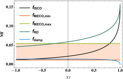
Figure 1: The ringdown and damping frequencies $f_{\rm{RD}}$ and $f_{\rm{damp}}$, and the ISCO frequency are plotted as functions of the dimensionless Kerr parameter $\chi_{f}$ of a black hole, a negative sign of $\chi_{f}$ indicates that the orbital angular momentum points in the opposite direction as the spin of the (final) black hole. Also plotted are the maximal and minimal MECO frequencies across the non-precessing parameter space (the maximum occurs for equal black holes with maximal component spins aligned with the orbital angular momentum, and the minimum for the extreme mass ratio limit with maximal anti-aligned component spins.

The loss of accuracy and gradual breakdown of the post-Newtonian series expansion for high frequencies as the merger is approached also determines the frequency regime where numerical solutions are required to provide unambiguous approximate solutions and error estimates. The computational cost of such simulations increases drastically as the initial frequency is lowered, the leading order post-Newtonian estimate for the time to merger $T$ for start frequency $f_{0}$ is

$$T\propto\frac{f_{0}^{-8/3}}{\eta}.$$ (30)

Covering densely the parameter space that we want to model with numerical relativity waveforms with start frequencies lower than the sensitive band of our detectors is still prohibitively expensive, and we will thus use “hybrid" waveforms as our input data set, where numerical relativity waveforms are appropriately glued to an inspiral description derived from the post-Newtonian expansion, as discussed below in Sec. III.

III Input waveforms

The primary input data we use for developing, calibrating, and evaluating the IMRPhenomXAS waveform model is the set of hybrid waveforms described in Husa et al. (2020). These waveforms are constructed by appropriately gluing together numerical waveforms, which cover the last orbits, merger and ringdown, with an inspiral model. For comparable masses up to mass ratio 18, the numerical waveforms have been computed by solving the full Einstein field equations using the methods of numerical relativity. The inspiral model is taken to be an EOB resummation of post-Newtonian waveforms. For extreme mass ratios we use numerical solutions for linearized gravitational waves in a Kerr background, sourced by EOB dynamics, as described below.

The EOB approach provides a framework to extend the validity of post-Newtonian results Buonanno and Damour (1999a, b) with resummation techniques, and to incorporate additional information, such as a calibration to numerical relativity results, which has lead to families of time-domain models for the complete waveform, from inspiral to ringdown Taracchini et al. (2014); Bohé et al. (2017); Nagar et al. (2018). Here we use the recent SEOBNRv4 Bohé et al. (2017) EOB model to hybridize with numerical relativity waveforms. For IMRPhenomD, the SEOBNRv2 approximant Taracchini et al. (2014) was used, removing however the calibrations to numerical relativity in order to decrease the dependence between the two models. Here we use the original calibrated SEOBNRv4 model, as our goal is to maximize the accuracy of the resulting waveform model.

SEOBNRv4 has in fact been calibrated to numerical waveforms, and describes the complete waveform from inspiral to ringdown. We could thus also augment our calibration data set with SEOBNRv4 waveforms in regions of the parameter space where numerical relativity waveforms are sparse. In the model presented here, we only use such SEOBNRv4 waveforms at low frequencies in the inspiral, i.e. well below the MECO frequency, where very little to no NR information is present. For the intermediate and merger-ringdown regions, only EOB-NR hybrids and test-particle hybrids are used to calibrate the waveform model.

The comparable mass numerical relativity waveforms used in the hybrid data set have been produced with SpEC Ossokine et al. (2013); Hemberger et al. (2013); Szilagyi et al. (2009); Scheel et al. (2009); Boyle et al. (2007); Mroué et al. (2013); Buchman et al. (2012)), which uses pseudo-spectral numerical methods and black-hole excision, as well as with the BAM Bruegmann et al. (2008); Husa et al. (2008) and Einstein Toolkit Babiuc-Hamilton et al. (2019) codes.

The BAM code solves the $3+1$ decomposed Einstein field equations using the $\chi$-variant Campanelli et al. (2006) of the moving-punctures implementation of the BSSN formulation Nakamura et al. (1987); Shibata and Nakamura (1995); Baumgarte and Shapiro (1999). Spatial derivatives are computed using sixth-order accurate finite differencing stencils Husa et al. (2008). Kreiss-Oliger dissipation terms converge at fifth order , and a fourth-order Runge-Kutta algorithm is used for the time evolution. BBH puncture initial data Brandt and Brügmann (1997); Bowen and York (1980) are calculated with a pseudo-spectral elliptic solver described in Ref Ansorg et al. (2004). The GWs are calculated using the Newman-Penrose scalar $\psi_{4}$ and extracted at a finite distance from the source.

The Einstein-Toolkit simulations use Bowen-York initial data Bowen and York (1980); Brandt and Brügmann (1997) computed using the TwoPunctures thorn Ansorg et al. (2004). Time evolution is performed using the $W$-variant Marronetti et al. (2008) of the BSSN formulation of the Einstein field equations as implemented by McLachlan Brown et al. (2009). The BHs are evolved using standard moving punctures gauge-conditions Baker et al. (2006); Campanelli et al. (2006). The lapse is evolved according to the $1+\log$ condition Bona et al. (1995) and the shift according to the hyperbolic $\tilde{\Gamma}$-driver Alcubierre et al. (2003). Simulations are performed using 8th order accurate finite difference stencils with Kreiss-Oliger dissipationGustaffsson et al. (1995). Adaptive mesh refinement is provided by Carpet Schnetter et al. (2004, 2006), with the wave-extraction zone being computed on spherical grids using the Llama multipatch infrastructure Pollney et al. (2011). Low eccentricity initial data is produced following the procedure outlined in Ramos-Buades et al. (2019). Further details will be given in Husa et al. (2020).

SpEC is a multi-domain pseudo-spectral code Lindblom et al. (2006); Szilagyi et al. (2009); Hemberger et al. (2013) that uses excision to remove the BH interiors, thereby removing the BH singularity from the computational domain. The code evolves the Generalised Harmonic coordinate formulation of the Einstein field equations Friedrich (1985); Pretorius (2005); Garfinkle (2002); Lindblom et al. (2006) with constraint damping. Initial data is constructed using the Extended Conformal Thin Sandwich (XCTS) equations York (1999); Pfeiffer and York (2003); Pfeiffer et al. (2003), with newer simulations typically choosing the conformal metric and trace of the extrinsic curvature to be a weighted superposition of two single BHs in Kerr-Schild coordinates Lovelace et al. (2008). Boundary conditions imposed on the excision boundaries ensure that these boundaries are apparent horizons Szilagyi et al. (2009); Scheel et al. (2009); Hemberger et al. (2013); Lindblom et al. (2006). Further details can be found in Boyle et al. (2019).

We used 186 waveforms from the public SXS catalog as of 2018 Mroué et al. (2013). After the release of the latest SXS collaboration catalog, Boyle et al. (2019), we extended the dataset to incorporate 355 SpEC simulations and updated the parameter space fits for the phase accordingly. We opted not to update the amplitude fits to incorporate the latest SpEC simulations as this is anticipated to have a smaller impact on the overall accuracy of the waveform model.

The 95 BAM waveforms consists of previously published and new waveforms. The Einstein Toolkit simulations have been recently produced by the authors. For further details on the BAM and Einstein Toolkit waveforms see Husa et al. (2020).

The key data sets that determine the calibration range of our waveform model are the BAM waveforms for a range of spins at mass ratio 1:18, high-spin BAM and SXS waveforms at mass ratios 4 and 8, and equal mass SXS data sets at very high spins of $-0.95$ and $+0.994$.

The coverage of the comparable mass parameter space is shown in Fig. 2.

As the computational cost of NR simulations diverges rapidly as $\eta\rightarrow 0$, no systematic NR simulations are available for mass ratios $q\geq 18$. This severely limits the parameter space against which we can calibrate a waveform model to NR. Constraining the asymptotic behaviour of the parameter space fits in the extreme-mass-ratio limit is essential for well-behaved extrapolation and to reduce uncertainty in the waveform model for intermediate-mass-ratio binaries, where NR coverage is extremely sparse. For many of the coefficients appearing in our waveform model, no fully analytical knowledge, with complete spin dependence, is available and we instead opt to constrain the fits by calibrating against semi-analytical waveforms in the test-particle limit.

As in Keitel et al. (2017), the simulations for BBH mergers in the test-particle limit are produced using Teukode Harms et al. (2014, 2016a, 2016b), which combines a semi-analytical description of the dynamics with a time-domain numerical approach for computing the full multipolar waveform. The dynamics of the binary are prescribed using EOB dynamics, where conservative geodesic motion has been augmented with a linear-in-$\eta$ radiation reaction Nagar et al. (2007); Damour and Nagar (2007). This makes use of the factorized and resummed circularized waveform introduced in Damour et al. (2009); Pan et al. (2014) and uses PN information up to 5.5PN. The fluxes are computed by solving the Regge-Wheeler-Zerilli (RWZ) $1+1$ equations (non-spinning) or the Teukolsky $2+1$ equations (spinning). These equations are solved in the time domain using a hyperboloidal foliation and horizon-penetrating coordinates that allow for the unambiguous extraction of radiation at $\mathscr{I}^{+}$ (future null infinity) Bernuzzi et al. (2011a, b); Harms et al. (2014).

As with the NR simulations detailed above, the test-particle waveforms are hybridized against a longer EOB inspiral. For the calibration of IMRPhenomXAS, we use two sets of waveforms: one set at $q=200$ and the other set at $q=1000$. The spin of the primary BH spans an interval $\left[-0.9,0.9\right]$ and the secondary BH is taken to be non-spinning.

The waveforms in the test-particle limit should only be treated as approximate as $\mathcal{O}(\eta)$ effects are neglected in the conservative dynamics and the 5PN-accurate EOB-resummed analytical multipolar waveforms, used to build the radiation reaction force, show relatively poor performance. A more detailed discussion on some of the observed discrepancies between the comparable-mass limit and the extreme-mass-ratio limit will be given below.

A recently proposed framework for the factorization and resummation of the residual waveform amplitudes Nagar and Shah (2016); Messina et al. (2018); Nagar et al. (2019a) is expected to improve the self-consistency of the test-particle waveforms and hence the self-consistency of the calibration. A detailed discussion of different approaches to resummation and the radiation reaction was presented in Nagar et al. (2019b). A detailed study of the consistency of IMRPhenomXAS in the test-particle limit will be presented elsewhere.

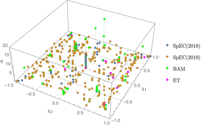
Figure 2: The mass ratio and spins for the NR waveforms used in the calibration of IMRPhenomXAS. SXS simulations are shown in blue (Mroué et al. (2013)) and orange (Boyle et al. (2019)), BAM simulations in green and Einstein Toolkit simulations in pink.

IV Mapping Phenomenological Coefficients to Physical Parameters

The model here has 8 amplitude coefficients and 13 phase coefficients, meaning that there are 21 phenomenological coefficients that must be mapped to the physical 3D parameter space $(\eta,\hat{S},\delta\chi)$, where $\hat{S}$ is an effective spin parameterisation of our choice and $\delta\chi=\chi_{1}-\chi_{2}$ is the linear-in-spin difference. The mapping procedure detailed here is a generalisation of the approach taken in previous phenomenological models and pioneered in fits to the radiated energy, final mass and final spin Jiménez-Forteza et al. (2017); Keitel et al. (2017). Here we use a hierarchical, bottom-up approach to calibrate fits to numerical relativity waveforms. As in previous post-Newtonian studies, the dominant parameter dependencies are on the mass ratio and effective spin parameterisations. The remaining unequal spin contribution is sub-dominant and can be effectively modelled by working to linear order in the spin difference. We provide a representative example of this workflow in Sec. VIII and a flowchart of the logic behind the hierarchical fitting procedure is shown in Fig. 3.

IV.1 Collocation Points

Direct calibration of the phenomenological coefficients to the hybrid data can often be problematic due to poor numerical conditioning. This is notable during inspiral, where both poor convergence and eventual breakdown of the PN series can lead to numerical instabilities for the pseudo-PN coefficients used to capture higher frequency behaviour. Such coefficients typically alternate in sign leading to significant numerical cancellations that must be captured accurately across the parameter space in order for the model to remain accurate.

In constructing a phenomenological waveform model, the aim is to calibrate a model for the amplitude or phase within a given domain. Often this reduces to constructing a polynomial fit, $P_{n}(x)$, to the hybrid data $f(x)$. As stated by the Weierstrass theorem Weierstrass (1885), for any continuous real valued function on an interval $\left[a,b\right]$, there exists a polynomial $P_{n}(x)$ with $\epsilon>0$ such that for all $x\in\left[a,b\right]$ we have $|f(x)-p(x)|<\epsilon$. However, a well known caveat to this theorem is that the result is highly dependent on the set of polynomials used and on their convergence. In particular, use of equidistant nodes when constructing $P_{n}(x)$ can lead to oscillatory divergences from $f(x)$ as we increase the degree of the polynomial. This is known as Runge’s phenomena and results in unphysical oscillations that can impact the accuracy of the model. In order to help alleviate such issues, there are a number of possible options. For instance, we could help tame oscillatory behaviour by fitting to a lower degree polynomial or we could construct multiple overlapping subintervals constructed with low-degree polynomials, i.e. piecewise polynomial interpolation. Instead, the strategy adopted here, and in García-Quirós et al. (2020a), is to choose the interpolation nodes $\{x^{i}\}^{n}_{i=0}$ such that the maximum error $||e_{n}(x)||_{\rm{\infty}}$ is minimized. This can be achieved by selecting $(n+1)$ sample points for the polynomial $P_{n}(x)$ at the roots of the Chebyshev polynomial

$$x_{k} =\cos\left[\frac{(2k+1)\pi}{2n}\right].$$ (31)

There are a few key advantages to using Chebyshev nodes when constructing such phenomenological fits. First, the error will be the smallest for all polynomials of degree $n$. Secondly, the error can often be more uniformly distributed over the interval in which we perform the fit. Finally, the error decreases exponentially with $n$, leading to spectral convergence of the fit

$$||e_{n}(x)|| \leq\frac{||f^{(n+1)}||_{\rm{\infty}}}{2^{n}(n+1)!}.$$ (32)

In contrast, the error from using equidistant nodes scales approximately as $||f(x)-P_{n}(x)||\propto\mathcal{O}(2^{n})$. For these reasons, we find it optimal to use collocation points evaluated at the Chebyshev nodes in the domain of interest.

The value of these collocation points is then fit across the entire parameter space using the hierarchical procedure discussed in the next section. Using the values of the collocation points, or their differences, we can reconstruct the underlying phenomenological ansatz by solving a system of linear equations using standard methods, such as an LU factorization.

Figure 3: Flowchart for the hierarchical parameter space fits, taken from Fig. 1 of Jiménez-Forteza et al. (2017). The starting point are one-dimensional sub-manifolds, taken to be the equal mass and spin limit and the non-spinning limit. The next step is to use a given spin parameterisation to perform an expansion about the 1D fits. Finally, the residuals between the data and the 2D fits are used to fit for unequal spin contributions.

IV.2 Hierarchical Fitting Procedure: One-Dimensional Subspace Fits

The hierarchical fits are performed by first sampling the non-spinning parameter space, as this is the simplest and best-sampled subspace in the NR data set. All fits are constructed using Mathematica’s NonlinearModelFit function. We use both polynomial and rational ansätze. As in Jiménez-Forteza et al. (2017); Keitel et al. (2017), high-dimensional polynomials are used to construct a Padé approximant to the desired order, with the coefficients of the approximant being used as the starting values for the rational-function fits. The use of Padé approximants to pre-condition the NonLinearModelFit helps to alleviate issues related to non-convergence, which can arise due to singularities in the rational function. Following Jiménez-Forteza et al. (2017); Keitel et al. (2017), rational functions with a numerator of polynomial order $m$ and a denominator of polynomial order $k$ will be denoted as an ansatz of order $(m,k)$. The use of rational functions offers numerous advantages to high-dimensional polynomials. In particular we find that rational functions are smoother, less prone to unphysical oscillations and extrapolate in a more controlled manner.

IV.3 Hierarchical Fitting Procedure: Two-Dimensional Subspace Fits

The next step is to construct the two-dimensional fits spanning the $(\eta,\hat{S})$ subspace. The ansatz from the 1D fits will be supplemented with a polynomial of order $J$ in order to capture the 2D curvature associated to $\hat{S}$-dependent terms via

$$b_{i}\rightarrow b_{i}\displaystyle\sum^{j=J}_{j=0}\,f_{ij}\,\eta^{j}.$$ (33)

The general 2D ansatz for a phenomenological coefficient is therefore

$$\lambda(\eta,\hat{S})=\lambda(\eta,0)\;-\;\lambda(0.25,0)\;+\;\lambda(0.25,\hat{S},f_{ij}).$$ (34)

The order to which we expand in $\eta$ is dependent upon the behaviour of the phenomenological coefficient that is being fitted. Typically we find that expanding to third order in $\eta$ ($J=3$) is the lowest order that leaves sufficient freedom to incorporate the constraints from the 1D fits and the extreme mass ratio limit as well as to adequately capture all the features of the data set. At higher order in $\eta$, numerous pathologies outside the calibration regime can start to develop, leading to a significant degradation in the performance of the calibrated model. In order to avoid potential singularities, appropriate care must be taken to remove pathological coefficients from the denominator of the rational ansatz.

IV.4 Hierarchical Fitting Procedure: Unequal Spin Contributions and 3D Fits

The final stage in the hierarchical approach is to incorporate the subdominant effect of unequal spins. Here we parameterise this effect by $\Delta\chi=\chi_{1}-\chi_{2}$. The residuals are defined by subtracting the 2D equal spin fit from the fit against the unequal-spin NR cases:

$$\Delta\lambda\,(\eta,\hat{S},\Delta\chi) =\lambda\,(\eta,\hat{S},\Delta\chi)-\lambda\,(\eta,\hat{S}).$$ (35)

This procedure can be done at discrete points in the symmetric mass ratio provided that sufficient unequal spin NR simulations are available.

At a given mass ratio, the residuals form a 2D surface $(\hat{S},\Delta\chi,\Delta\lambda)$ which can be used to informatively construct an ansatz for the unequal spin effects. As with many aspects of phenomenological waveform modelling, insight can be taken from studying the structure of the post-Newtonian equations. For example, if we consider the next-to-leading order (NLO) spin-orbit (SO) contribution to the flux

$$\mathcal{F}_{\rm SO}^{\rm NLO} \propto\left(-\frac{9}{2}+\frac{272}{9}\eta\right)$$ (36)

$$\qquad\sqrt{1-4\eta}\;\left(-\frac{13}{16}+\frac{43}{4}\eta\right)\;\Sigma_{\ell},$$

where

$$S_{\ell} =m^{2}_{1}\;{\chi}_{1\ell}\;+\;m^{2}_{2}\;{\chi}_{2\ell},$$ (37)

$$\Sigma_{\ell} =\left(\;m_{2}\;{\chi}_{2\ell}\;-\;m_{1}\;{\chi}_{1\ell}\;\right).$$ (38)

By inspection, the linear-in-spin difference contribution is killed by a factor of $\delta=\sqrt{1-4\eta}$ in the equal mass limit. Away from equal masses, the unequal spin contribution is a simple polynomial function in $\eta$. By comparison, the leading-order (LO) spin-spin (SS) term is given by

$$\mathcal{F}^{\rm LO}_{\rm SS} \propto x^{2}\left({8S_{\ell}^{2}}+8\;\delta\;\Sigma_{\ell}\;S_{\ell}+\left(\frac{33}{16}-8\eta\right)\;\Sigma_{\ell}^{2}\right),$$ (39)

where in the equal mass limit the mixed term $\Sigma_{\ell}\,S_{\ell}$ is killed by a factor of $\delta$ but we still have a non-vanishing quadratic-in-spin-difference term $\Sigma^{2}_{\ell}$.

In practice, we find that the 2D surfaces are typically close to flat, suggesting that the unequal spin effects are dominanted by a linear dependence on $\Delta\chi$ and a possible mixture term $\hat{S}\Delta\chi$. This linear dependence will break down in the equal mass limit as, under an exchange of $\chi_{1}$ and $\chi_{2}$, terms linear in $\Delta\chi$ will vanish. In this limit, the surface is approximately parabolic and well-modelled by a quadratic term.

Based on the above considerations, we use a general ansatz with three spin-difference terms

$$\Delta\lambda(\eta,\hat{S},\Delta\chi)=A_{1}(\eta)\Delta\chi+A_{2}(\eta)\Delta\chi^{2}+A_{3}(\eta)\Delta\chi\,\hat{S}.$$ (40)

The resulting full 3D ansatz is therefore given by

$$\lambda(\eta,\hat{S},\Delta\chi) =\lambda(\eta,\hat{S})+\Delta\lambda(\eta,\hat{S},\Delta\chi).$$ (41)

Additional higher order terms in the effective spin or spin difference are not used as there is no motivation from either PN or visual inspection of the residuals. In addition, the intrinsic error of the NR simulations begins to dominate and caution is required to ensure that we do not overfit noisy data. As a check, we follow the approach in Jiménez-Forteza et al. (2017) and perform four fits in $\Delta\chi$ for the values of $A_{i}$: linear, linear+quadratic, linear+mixed and the sum of all three contributions.

IV.5 Choice of Spin Parameterisation

A choice that must be made when constructing the fits across the parameter space is the spin parameterisation, $\hat{S}$, employed. The choice of parameterization can help minimize errors when building fits on a subspace of the data. One of the most widely used spin parameterizations is the effective aligned spin Damour (2001); Racine (2008); Ajith et al. (2011)

$$\chi_{\rm{eff}} =\frac{m_{1}\chi_{1}+m_{2}\chi_{2}}{M}.$$ (42)

This choice was made in early Phenomenological waveform models IMRPhenomB Ajith et al. (2011) and IMRPhenomC Santamaria et al. (2010). In IMRPhenomD, an alternative spin parameterization was used based on the reduced spin parameter, that describes the leading order spin-orbit term at 1.5PN Poisson and Will (1995); Ajith (2011)

$$\chi_{\rm{PN}} =\chi_{\rm{eff}}-\frac{38\eta}{113}\left(\chi_{1}+\chi_{2}\right),$$ (43)

normalized to $\left[-1,1\right]$ for any mass ratio

$$\hat{\chi}_{\rm{PN}} =\frac{\chi_{\rm{PN}}}{1-76\eta/113}.$$ (44)

This PN motivated parameterization is particularly suited to use in IMR waveform models Pürrer et al. (2013) and was also found to best capture spin-orbit contributions to the binding energy Ossokine et al. (2018). We will adopt $\hat{\chi}_{\rm{PN}}$ as our spin parameterization of choice for the inspiral regime.

For the final state, however, the underlying physics is best captured by the linear spin combination $S_{1}+S_{2}$. We therefore find it useful to employ an effective total spin parameter

$$\hat{S}_{\rm{tot}} =\frac{S}{m^{2}_{1}+m^{2}_{2}},\quad\textrm{with}\quad S=m^{2}\chi_{1}+m^{2}\chi_{2},$$ (45)

which was found to work well for final-state quantities Husa et al. (2016); Jiménez-Forteza et al. (2017). In IMRPhenomXAS, we will use $\hat{S}$ to parameterize the fits to the intermediate and merger-ringdown coefficients. A detailed study of the impact of different spin parameterizations is beyond the scope of this paper.

V Matching Regions

Following the strategy adopted in previous phenomenological waveform models Ajith et al. (2008, 2011); Santamaria et al. (2010); Husa et al. (2016); Khan et al. (2016), we split the waveform into three frequency regions and model each of these regimes separately. This is done for both the amplitude and the phase derivative. In this section we define these regions and explicitly highlight the calibration range used in determining the fits as well as the transition windows used when reconstructing the phenomenological model. These regions are highlighted in Fig. 4.

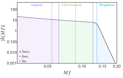
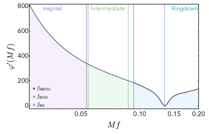
Figure 4: Transition regions for the amplitude and phase derivative $\varphi^{\prime}=\partial_{f}\varphi(f)$. The purple shaded area shows the inspiral region, green shaded the intermediate and the blue shaded the merger-ringdown. The three colored lines show the MECO (purple), ISCO (green) and ringdown (blue) frequencies respectively.

V.1 Inspiral

Two of the key improvements of IMRPhenomXAS over IMRPhenomD concern the frequency region over which the model is calibrated to the hybrid data. For IMRPhenomD this region was

$$0.0035\leq Mf\leq 0.018\,.$$ (46)

In IMRPhenomXAS the lower frequency has been reduced to

$$f_{0}=0.0026\,$$ (47)

which corresponds to lowering the starting frequency from $71.1Hz$ to $52.8Hz$ for a binary of total mass of 10 $M_{\odot}$, or to lowering the binary mass for which the calibration completely covers frequencies above 10 Hz from $71.1M_{\odot}$ to $52.8M_{\odot}$. We find that this change significantly improves matches between hybrids and the model for lower masses. The reason for not lowering the starting frequency further has been twofold: First, we build our hybrid waveforms in the time domain, and need to Fourier transform the hybrids on an equispaced frequency grid. In order to simplify our setup, we choose this frequency grid to be the same for all our waveforms. In order to achieve sufficient resolution at high frequencies, we choose a time step of $t/M=0.5$. The start frequency is chosen to conveniently fit the complete hybrid generation in the time and frequency domain into the RAM available on a laptop for mass ratios up to about 500, as described in Husa et al. (2020). Allowing for windowing and robustly cutting away different types of artifacts, restricts the low frequency limit that can be achieved. In future editions of the model, a more flexible approach will be used, to further reduce the start frequency. The second reason is that a further reduction of start frequency would only be useful with further studies of how to best model the inspiral (e.g. regarding the order of pseudo-PN terms used, and the number of collocation points used). These studies are outside the scope of the present paper, but will be required for a more accurate representation of the extreme mass ratio limit, and possibly for further increases in accuracy.

In IMRPhenomD, the maximal frequency for the inspiral description in terms of a modified post-Newtonian ansatz, was also fixed, irrespective of the binaries mass ratio or spin. In the extreme mass ratio case, an appropriate choice of transition frequency is given by the ISCO (innermost stable circular orbit) frequency, which can be evaluated in closed form, and ranges from $Mf\approx 0.006$ for inspiral into an extreme Kerr black hole with orbital angular momentum anti-aligned with the spin of the large black hole, to $Mf\approx 0.08$ for the aligned case. A fixed transition frequency from the inspiral to the intermediate regime is thus clearly not appropriate for extreme mass ratios, but also not for comparable masses where the dynamical range is smaller.

A natural termination frequency for the inspiral, which also applies to comparable masses, can be based on the minimum energy circular orbit (MECO) frequency. In a standard binary black hole inspiral, the orbital energy will gradually decrease until it reaches some minimum. The MECO is defined to be the orbit at which the orbital energy reaches its minimum value. Naturally, the MECO is implicitly tied to the PN order under consideration, which can be problematic in the extreme mass ratio limit where the PN approximation is poorly convergent. In order to alleviate such problems, Cabero et al. (2017) implemented a hybrid-MECO in which test-particle dynamics are folded into the PN approximation in order to provide a well-defined MECO condition valid for all spins. Schematically, the hybrid energy is constructed by replacing the test-particle limit of the PN energy with the exact orbital energy per unit mass for a test-particle around a Kerr black hole Cabero et al. (2017)

$$E^{\rm{Hybrid}}=\frac{E^{\rm{n-PN}}}{\eta}-\left(\displaystyle\sum^{x=2n}_{x=0}E^{\rm{Kerr}}(v^{x})\right)+E^{\rm{Kerr}}$$ (48)

where

$$E^{\rm{Kerr}}=\left(\frac{1-2w+\chi w^{3/2}}{\sqrt{1-3w+2\chi w^{3/2}}}-1\right),$$ (49)

and $w=v^{2}/(1-\chi v^{3})^{2/3}$. This expression was shown to have a minimum for currently known PN orders. In practice, we use a phenomenological fit to the hybrid-MECO as a natural PN approximation to the end of the inspiral. This alleviates the necessity of performing a root-finding operation when evaluating the waveform model.

The inspiral calibration range for the amplitude $(A)$ and the phase $(\varphi)$ is taken to be

$$f^{\varphi}_{C,\rm{Ins}} \in\left[0.0026,1.02f_{\rm{MECO}}\right],$$ (50)

$$f^{A}_{C,\rm{Ins}} \in\left[0.0026,1.025f^{A}_{T}\right],$$ (51)

where the $C$ explicitly denotes the calibration domain and

$$f^{A}_{T} =f_{\rm{MECO}}+\frac{1}{4}\left(f_{\rm{ISCO}}-f_{\rm{MECO}}\right).$$ (52)

However, when building the waveform, the inspiral region interval is defined by

$$f^{\varphi}_{\rm{Ins}} \in\left(0,f_{\rm{MECO}}-\delta_{R}\right)$$ (53)

$$f^{A}_{\rm{Ins}} \in\left(0,f^{A}_{T}\right],$$ (54)

where

$$\delta_{R} =0.03\left(f^{\varphi}_{R,3}-f_{\rm{MECO}}\right),$$ (55)

$$f^{\varphi}_{T} =0.6\left(\frac{1}{2}f_{\rm{RD}}+f_{\rm{ISCO}}\right).$$ (56)

The inspiral region corresponds to the purple-shaded region in Fig. 4.

V.2 Intermediate Regime

The intermediate regime is introduced in order to phenomenologically bridge the gap between the post-Newtonian regime and the perturbative black hole ringdown regime. The start of this region is determined by the breakdown of post-Newtonian theory and the end of the region is set relative to the ISCO and ringdown frequencies. This enables us to implicity incorporate a natural hierarchy of frequencies in a standard binary black hole inspiral: $f_{\rm{MECO}}<f_{\rm{ISCO}}<f_{\rm{ring}}$.

For the intermediate region, the calibration domain is taken to be

$$f^{\varphi}_{C,\rm{Int}} \in\left[f_{\rm{MECO}}-\delta_{R},f^{\varphi}_{T}+0.5\delta_{R}\right],$$ (57)

$$f^{A}_{C,\rm{Int}} \in\left[0.98f^{A}_{T},1.02f_{\rm{peak}}\right],$$ (58)

where $f_{\rm{peak}}$ is the analytical location of the peak of the ringdown Husa et al. (2016); Khan et al. (2016)

$$f_{\rm{peak}} =\left|f_{\rm{RD}}+f_{\rm{damp}}\sigma\frac{\sqrt{1-\lambda}-1}{\lambda}\right|.$$ (59)

The intermediate interval when building the waveform is defined by

$$f^{\varphi}_{\rm{Int}} \in\left[f_{\rm{MECO}}-\delta_{R},f^{\varphi}_{T}+\delta_{R}\right]$$ (60)

$$f^{A}_{\rm{Int}} \in\left(f^{A}_{T},f_{\rm{peak}}\right].$$ (61)

The intermediate region corresponds to the green-shaded region in Fig. 4.

V.3 Merger-Ringdown Regime

Finally, the merger-ringdown regime is particularly well described in terms of the ringdown and damping frequency of the remnant BH. The calibration interval for the merger-ringdown is taken to be

$$f^{\varphi}_{C,\rm{MR}} \in\left[0.985f^{\varphi}_{T},f_{\rm{RD}}+1.25f_{\rm{damp}}\right],$$ (62)

$$f^{A}_{C,\rm{MR}} \in\left[f_{\rm{RD}}-\frac{(1+4\eta)}{5}f_{\rm{damp}},f_{\rm{RD}}+3.25f_{\rm{damp}}\right],$$ (63)

note that the factor of $(1+4\eta)$ has been added to help control the fits in the extreme-mass-ratio limit, where the amplitudes at the peak of the rescaled data can become particularly flat and no clear merger-ringdown can be defined in a morphological sense.

The merger-ringdown frequency interval when reconstructing the waveform is defined by

$$f^{\varphi}_{\rm{MR}} \in\left(f^{\varphi}_{T},0.3Mf\right),$$ (64)

$$f^{A}_{\rm{MR}} \in\left(f_{\rm{peak}},0.3Mf\right),$$ (65)

where $0.3Mf$ is an arbitrary high-frequency cutoff frequency implemented for IMRPhenomXAS in LAL. The merger-ringdown region corresponds to the blue-shaded region in Fig. 4.

VI Amplitude Model

When calibrating the amplitude model of IMRPhenomXAS to the hybrid data, we factor out the leading order PN behaviour $f^{-7/6}$. We opt to normalize the data such that as $f\rightarrow 0$ the data tends to unity. This normalization is motivated by the Newtonian limit

$$\lim_{f\rightarrow 0}\,\left[f^{7/6}\,A_{\rm{PN}}(f) \right]\rightarrow\sqrt{\frac{2\eta}{3\pi^{1/3}}},$$ (66)

with the resulting normalization factor being

$$A_{0}\equiv\sqrt{\frac{2\eta}{3\pi^{1/3}}}\;f^{-7/6}.$$ (67)

VI.1 Inspiral

The inspiral model is based on a PN re-expanded TaylorF2 amplitude augmented with pseudo-PN terms that are calibrated to the hybrid data

$$A_{\rm{Ins}}(f)=A_{\rm{PN}}+A_{0}\displaystyle\sum_{i=1}^{3}\,\rho_{i}\,(\pi\,f)^{(6+i)/3},$$ (68)

where $A_{\rm{PN}}$ constitutes the known PN terms

$$A_{\rm{PN}}(f)=A_{0}\displaystyle\sum_{i=0}^{6}\,\mathcal{A}_{i}\,(\pi\,f)^{i/3},$$ (69)

and $\rho_{i}$ are the pseudo-PN coefficients, where $A_{0}$ is the normalization factor corresponding to the leading order PN term $f^{-7/6}$. An example of the calibrated inspiral amplitude compared to the hybrid data is shown in Fig. 5.

The pseudo-PN coefficients are constructed by calibrating collocation points at the nodes

$$\{0.5,0.75,1.0\}f_{\rm{MECO}},$$ (70)

and analytically solving the system of equations generated by evaluating the pseudo-PN terms in Eq. 69 at the above nodes.

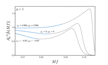
Figure 5: Amplitude inspiral fit for a series of $q=1$ SXS simulations.

VI.2 Intermediate

As an example of the modularity of IMRPhenomXAS, we implement two different models for the intermediate amplitude. The first model is based on the inverse of a fourth-order or fifth-order polynomial

$$A_{\rm{Int}}=\frac{A_{0}}{\alpha_{0}+\alpha_{1}f+\alpha_{2}f^{2}+\alpha_{3}f^{3}+\alpha_{4}f^{4}},$$ (71)

and the second model on the inverse of a fifth-order polynomial

$$A_{\rm{Int}}=\frac{A_{0}}{\alpha_{0}+\alpha_{1}f+\alpha_{2}f^{2}+\alpha_{3}f^{3}+\alpha_{4}f^{4}+\alpha_{5}f^{5}}.$$ (72)

For an ansatz with $n$ coefficients, we require $n$ pieces of information in order to reconstruct the underlying function. For the fifth-order polynomial, the function requires six input parameters, given by the value of the amplitude at two collocation points together with four boundary conditions: two for the amplitude and two for the first derivative of the amplitude. The amplitude is therefore $C^{1}$ continuous by construction. A similar argument holds for the fourth-order function, though using 5 coefficients. The collocation points used for both models are detailed in Tables 1 and 2. For the fifth-order polynomial, the coefficients $\alpha_{i}$ are the solution to the system of equations

$$A_{\rm{Ins}}(f_{1}) =v_{1},$$ (73)

$$A_{\rm{Hyb}}(f_{2}) =v_{2},$$ (74)

$$A_{\rm{Hyb}}(f_{3}) =v_{3},$$ (75)

$$A_{\rm{MR}}(f_{4}) =v_{4},$$ (76)

$$A^{\prime}_{\rm{Ins}}(f_{1}) =d_{1},$$ (77)

$$A^{\prime}_{\rm{MR}}(f_{4}) =d_{4}.$$ (78)

For the fourth-order polynomial, the system of equations is analagous to Khan et al. (2016)

$$A_{\rm{Ins}}(f_{1}) =v_{1},$$ (79)

$$A_{\rm{Hyb}}(f_{2}) =v_{2},$$ (80)

$$A_{\rm{MR}}(f_{4}) =v_{3},$$ (81)

$$A^{\prime}_{\rm{Ins}}(f_{1}) =d_{1},$$ (82)

$$A^{\prime}_{\rm{MR}}(f_{3}) =d_{3}.$$ (83)

The fifth-order ansatz allows us to capture more dramatic features in the amplitude morphology, which is particular important as we extend to higher mass ratios. For aligned-spin binaries, the system is highly adiabatic and there are many quasi-circular orbits before the smaller black hole plunges into the larger black hole. For anti-aligned spins, the system is not adiabatic and the system evolves through to the plunge phase much quicker, especially at high mass ratios. For the un-adiabatic case, the binary shows a distinct morphology in which the amplitude drops as we rapidly transition from the inspiral to the merger-ringdown. A comparison between the fourth-order and fifth-order intermediate ansatz against $q=8$ hybrid data is shown in Fig. 6.

For the remainder of this paper, we will work with the fifth-order intermediate ansatz unless otherwise stated.

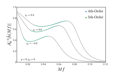
Figure 6: The fit to the intermediate amplitude using a 4th-order and 5th-order ansatz using 3 SXS simulations at $q=8$. The 5th-order ansatz is able to more accurately fit the features in the waveform but has poor extrapolation compared to the 4th order ansatz.

Table 1: Location of collocation points $f_{i}$ for the fifth-order intermediate ansatz. The coefficients $v_{1},v_{4},d_{1},d_{4}$ are constrained by the inspiral and merger-ringdown model. The free coefficients $v_{2}$ and $v_{3}$ must be fit to the data.

Collocation Points	Value	Derivative
$f_{1}=f^{W}_{1}$	$v_{1}=A_{\rm{Ins}}(f_{1})$	$d_{1}=A^{\prime}_{\rm{Ins}}(f_{1})$
$f_{2}=(f^{A}_{T}+f_{\rm{peak}})/3$	$v_{2}=A_{\rm{Hyb}}(f_{2})$
$f_{3}=2(f^{A}_{T}+f_{\rm{peak}})/3$	$v_{3}=A_{\rm{Hyb}}(f_{3})$
$f_{4}=f_{\rm{peak}}$	$v_{4}=A_{\rm{MR}}(f_{4})$	$d_{4}=A^{\prime}_{\rm{MR}}(f_{4})$

Table 2: Location of collocation points $f_{i}$ for the fourth-order intermediate ansatz. The coefficients $v_{1},v_{3},d_{1},d_{3}$ are constrained by the inspiral and merger-ringdown model, whereas $v_{2}$ must be fit to the data.

Collocation Points	Value	Derivative
$f_{1}=f^{A}_{T}$	$v_{1}=A_{\rm{Ins}}(f_{1})$	$d_{1}=A^{\prime}_{\rm{Ins}}(f_{1})$
$f_{2}=(f^{A}_{T}+f_{\rm{peak}})/2$	$v_{2}=A_{\rm{Hyb}}(f_{2})$
$f_{3}=f_{\rm{peak}}$	$v_{3}=A_{\rm{MR}}(f_{3})$	$d_{3}=A^{\prime}_{\rm{MR}}(f_{3})$

VI.3 Merger-Ringdown

The merger-ringdown ansatz is modelled using a deformed Lorentzian, corresponding to the Fourier transform of a two-sided exponential decay function. The ansatz adopted is given by Husa et al. (2016); Khan et al. (2016)

$$A_{\rm{MR}} =\left[\frac{a_{R}\;(f_{\rm{damp}}\;\sigma)}{(f-f_{\rm{RD}})^{2}+(f_{\rm{damp}}\;\sigma)^{2}}\right]e^{-\lambda(f-f_{\rm{RD}})/(f_{\rm{damp}}\;\sigma)}.$$ (84)

Unlike the other two regions, here we choose to calibrate $\lambda$ and $\sigma$ directly. In order to solve the amplitude coefficient $a_{R}$, we further calibrate a collocation point at the defined at $f_{\rm{peak}}$. Together with $\lambda$ and $\sigma$, we can use the collocation point to solve a trivial system of equations for $a_{R}$. An example of the ringdown fit applied to the BAM $q=18$ data is shown in Fig. 7.

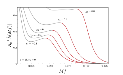
Figure 7: The fit to the merger-ringdown amplitude for 5 BAM simulations at $q=18$ corresponding to spins on the primary BH of $\chi_{1}\in\{-0.8,-0.4,0,0.4,0.8\}$. The secondary BH is non-spinning.

VII Phase Model

VII.1 Inspiral

The inspiral phase model is based on TaylorF2, derived under the stationary phase approximation, augmented with pseudo-PN coefficients that are calibrated to the hybrid data. The full TaylorF2 phase can be written as

$$\varphi_{\rm{Ins}} =\varphi_{\rm{TF2}}(Mf;{\bm{{\theta}}})$$ (85)

$$\quad+\frac{1}{\eta}\Bigg{(}\sigma_{0}+\sigma_{1}f+\frac{3}{4}\sigma_{2}f^{4/3}+\frac{3}{5}\sigma_{3}f^{5/3}$$

$$\qquad\qquad+\frac{1}{2}\sigma_{4}f^{6/3}+\frac{3}{7}\sigma_{5}f^{7/3}\Bigg{)}.$$

where $\varphi_{\rm{TF2}}$ is the analytically known TaylorF2 phase

$$\varphi_{TF2} =2\pi ft_{c}-\varphi_{c}-\frac{\pi}{4}+$$ (86)

$$\qquad\frac{3}{128\eta}\left(\pi Mf\right)^{-5/3}\displaystyle\sum^{7}_{i=0}\varphi_{i}\left({\bm{{\theta}}}\right)\,\left(\pi Mf\right)^{i/3},$$

and $\varphi_{i}({\bm{{\theta}}})$ are known PN coefficients that are functions of the intrinsic parameters of the binary. The coefficients $\sigma_{i}$ are the pseudo-PN coefficients that we calibrate against the hybrid dataset and supplementary SEOBNRv4 waveforms. A detailed discussion of the PN information used in IMRPhenomXAS is given in Appendix A.

The calibration of the pseudo-PN coefficients is performed by subtracting a given TaylorF2 approximant from the full hybrid phase and factoring out the leading order frequency power

$$\mathcal{R}_{\rm insp}(f)=f^{-8/3}\,\left(\varphi^{\prime}_{\rm Hybrid}(f)\,-\,\varphi^{\prime}_{\rm TF2}(f)\right).$$ (87)

By performing such a rescaling, we numerically condition the data such that we more accurately capture the un-modelled higher-PN contributions to the phase.

Note that, by construction, the calibrated pseudo-PN coefficients are implicitly tied to the specific TaylorF2 approximant used. If we incorporate additional analytical PN information, we would need to recalibrate the pseudo-PN coefficients on a case-by-case basis.

In this paper, we demonstrate the flexibility of the IMRPhenomXAS framework by producing four different calibrated inspiral models. The first two models adopt a canonical 3.5PN TaylorF2 phase using recent cubic-in-spin and quadratic-in-spin corrections Marsat (2015); Bohé et al. (2015) but use 4 or 5 pseudo-PN coefficients, with $\sigma_{0}$ being fixed by imposing $C^{1}$ continuity in the phase. The model with 4 additional coefficients requires 4 collocation points whereas the model with 5 additional coefficients requires 5 collocations points. The final set of models are all based on an extended TaylorF2 phase that incorporates some recent results at 4PN Damour et al. (2014); Bernard et al. (2016, 2017a); Damour and Jaranowski (2017); Bernard et al. (2017b); Marchand et al. (2018), 4.5PN Marchand et al. (2016) and a recently identified tail-induced, spin-spin term in the flux Messina et al. (2018). As before, we produce two variants with 4 and 5 pseudo-PN coefficients respectively.

The collocation points for this system are set by the Gauss-Chebyshev nodes. When using 4 collocation points, these nodes are given by

$$v_{i}^{\rm{Int}} =\left\{f_{L},\frac{1}{4}\delta^{\rm{Im}}_{\varphi},\frac{3}{4}\delta^{\rm{Im}}_{\varphi},f_{H}\right\}$$ (88)

where $f_{H}=1.02f_{\rm{MECO}}$, $f_{L}=0.0026$ and $\delta^{\rm{Im}}_{\varphi}=f_{H}-f_{L}$. For 5 collocation points, the nodes occur at

$$v_{i}^{\rm{Int}} =\Bigg{\{}f_{L},\frac{1}{2}\left(1-\frac{1}{\sqrt{2}}\right)\delta^{\rm{Im}}_{\varphi}+f_{L},f_{L}+\frac{1}{2}\delta^{\rm{Im}}_{\varphi},$$ (89)

$$\qquad\qquad\frac{1}{2}\left(1+\frac{1}{\sqrt{2}}\right)\delta^{\rm{Im}}_{\varphi}+f_{L},f_{H}\Bigg{\}}.$$

The location of the nodes when using 4 and 5 collocation points is demonstrated in Fig. 8, where we fit the residual ansatz in Eq. 87 to the hybrid data.

Unless otherwise stated, we adopt the canonical TaylorF2 ansatz with 4 pseudo-PN coefficients as the default inspiral model. The performance of the different inspiral models is discussed in Sec. IX and the mismatches, as defined in Eq. 116, shown in Fig. 16.

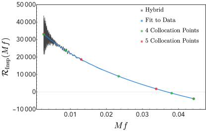
Figure 8: The pseudo-PN coefficients are fit to the the hybrid data by subtracting a given TaylorF2 approximant and factoring out the leading order frequency, $f^{-8/3}\left[\varphi^{\rm{Hyb}}(f)-\varphi^{\rm{TF2}}(f)\right]$. Such data conditioning helps the fit to capture the physical behaviour of the inspiral waveform up to the MECO frequency. The green circles denote the location of the sampling points for 3 psuedo-PN coefficients and the blue squares for 4 pseudo-PN coefficients. The sampling points are chosen based on a Gauss-Chebyshev aimed at reducing Runga’s phenomena near the boundaries. Here we use SXS-BBH-0153 hybridized against SEOBNRv4 as a representative example.

VII.2 Intermediate

We now consider the phenomenological intermediate region. As in Husa et al. (2016); Khan et al. (2016), we adopt a polynomial ansatz but add a Lorentzian term to smoothly match the phase to the merger-ringdown ansatz. As with the inspiral, we provide two models as an example of the modularity of IMRPhenomXAS. The functional form for the general ansatz used for the intermediate phase is

$$\eta\;\varphi^{\prime}_{\rm{Int}} =b_{0}+b_{4}f^{-4}+b_{3}f^{-3}+b_{2}f^{-2}+b_{1}f^{-1}$$ (90)

$$\qquad\qquad-\frac{4c_{0}\,a_{\varphi}}{(f-f_{\rm{RD}})^{2}+(2f_{\rm{damp}})^{2}},$$

where the terms in the Lorentzian are implicitly set by the merger-ringdown model. The first model adopts 4 collocation points and sets $b_{3}=0$. The second model uses 5 collocation points and retains all 5 coefficients $\{b_{0},b_{1},b_{2},b_{3},b_{4},b_{5}\}$. Unlike IMRPhenomD, we impose additional constraints on the intermediate ansatz and use the value of the inspiral and merger-ringdown fits respectively to determine the boundary collocation points. The 4-coefficient model therefore requires two calibrated collocation points and the 5-coefficient model 3 calibrated terms. The Gauss-Chebyshev nodes for 4 collocation points occur at

$$v_{i}^{\rm{Int}} =\left\{f_{L},\frac{1}{4}\delta^{\rm{Im}}_{\varphi},\frac{3}{4}\delta^{\rm{Im}}_{\varphi},f_{H}\right\},$$ (91)

where $f_{H}=f^{\varphi}_{T}+0.5\delta_{R}$, $f_{L}=f_{\rm{MECO}}-\delta_{R}$ and $\delta^{\rm{Im}}_{\varphi}=f_{H}-f_{L}$. Similarly, for the 5 collocation points, the nodes occur at

$$v_{i}^{\rm{Int}} =\Bigg{\{}f_{L},\frac{1}{2}\left(1-\frac{1}{\sqrt{2}}\right)\delta^{\rm{Im}}_{\varphi}+f_{L},f_{L}+\frac{1}{2}\delta^{\rm{Im}}_{\varphi},$$ (92)

$$\qquad\qquad\frac{1}{2}\left(1+\frac{1}{\sqrt{2}}\right)\delta^{\rm{Im}}_{\varphi}+f_{L},f_{H}\Bigg{\}}.$$

In order to help numerically condition the collocation points, we opted to fit the difference with respect to $v_{4}^{\rm{MR}}$, the value of the merger-ringdown phase at the ringdown frequency. Such a strategy is particularly beneficial when extrapolating to higher mass ratios and high-spin configurations, where the sparsity of available NR simulations can lead to poor constraints on the parameter space fits. For the 4-coefficient model, the two free coefficients are $v_{2}$ and $v_{3}$. We therefore require parameter space fits for

$$\delta_{2,\rm{RD}4} =v_{2}^{\rm{Im}}-v_{4}^{\rm{RD}},$$ (93)

$$\delta_{3,\rm{RD}4} =v_{3}^{\rm{Im}}-v_{4}^{\rm{RD}},$$ (94)

which could be used in conjunction with a fit for $v_{4}^{\rm{RD}}$ to reconstruct $v_{2}^{\rm{Im}}$ and $v_{3}^{\rm{Im}}$ respectively. In order to help tame unphysical behaviour at extremely large mass ratios and large spins, we use a weighted average between the above fit and a direct fit to $v^{\rm{Im}}_{2}$ in the final model

$$v^{\rm{Im}}_{2} =0.75(\delta_{2,\rm{RD4}}+v^{\rm{RD}}_{4})+0.25v^{\rm{Im}}_{2}.$$ (95)

An example of the reconstructed intermediate phase derivative against hybrid data, along with the collocation points used, is shown in Fig.9. Unless otherwise stated, we take the 5th order polynomial ansatz as the default model for the intermediate phase derivative.

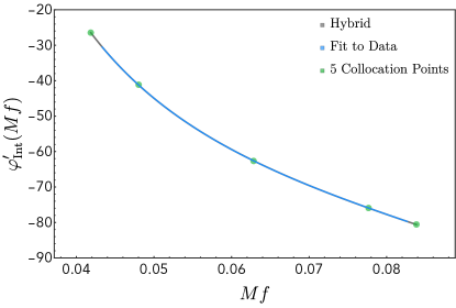
Figure 9: Phase derivative for SXS-BBH-0153 hybridized against SEOBNRv4 in the intermediate region and the fit to the data (blue) reconstructed from a system of collocation points (green).

VII.3 Merger-Ringdown

As in previous phenomenological waveform models, the ansatz for the merger-ringdown is based on a Lorentzian embedded in a background arising form the late inspiral and merger. In order to capture the steep inspiral gradient, negative powers of the frequency were added to the Lorentzian.

$$\eta\;\varphi^{{}^{\prime}}_{\rm{RD}} =c_{\rm{RD}}+\displaystyle\sum^{n}_{i}c_{i}\,f^{-{p_{i}}}+\frac{c_{0}\,a_{\varphi}}{f_{\rm{damp}}^{2}+(f-f_{\rm{RD}})^{2}}$$ (96)

In IMRPhenomD, the leading contribution was taken to be $p_{2}=2$ and an additional term $p_{3}=-1/4$ was added in order to reduce residuals across the parameter space. However, for IMRPhenomXAS, we find that we no longer require the coefficient $\alpha_{5}$, defined in Eq. 13 of Khan et al. (2016), to correct for the ringdown frequency. Using the recent recalibration of the final mass and spin fits in Jiménez-Forteza et al. (2017), the values of the ringdown and damping frequency are sufficiently accurate that we are able to drop this coefficient. This allows us to calibrate an additional coefficient without increasing the dimensionality of the fit. The inclusion of an additional polynomial coefficients is of particular importance in correctly modelling the gradient of the merger-ringdown in the extremal spin limit. For IMRPhenomXAS, we use three polynomial coefficients with powers of $-4,-2$ and $-1/3$ respectively.

As with the other regions, we use Gauss-Chebyshev nodes to fix the collocation points but set the 4th node to occur at the ringdown frequency. The ringdown frequency approximately correponds to the peak of the Lorentzian, as can be seen in Fig. 10. Whilst this may impact the optimality of reconstructing the underlying function, we find that $v_{4}^{\rm{MR}}$ is very-well conditioned and can be fit to high accuracy. The collocation points nodes for the merger-ringdown phase are therefore taken to be

$$v_{i} =\left\{f_{L},\frac{1}{2}\left(1-\frac{1}{\sqrt{2}}\right)\delta^{\rm{MR}}_{\varphi}+f_{L},f_{L}+\frac{1}{2}\delta_{\varphi}^{\rm{MR}},f_{\rm{RD}},f_{H}\right\},$$ (97)

where $f_{H}=f_{\rm{RD}}+\frac{5}{4}f_{\rm{damp}}$, $f_{L}=f^{\varphi}_{T}$ and $\delta^{\rm{MR}}_{\varphi}=f_{H}-f_{L}$.

An example of the reconstructed merger-ringdown phase derivative against hybrid data, along with the collocation points used, is shown in Fig.10. The fit detailed here is as implemented in the final model.

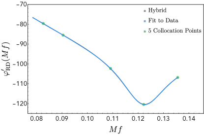
Figure 10: Phase derivative for SXS-BBH-0153 hybridized against SEOBNRv4 in the merger-ringdown region along with the fit to the data (blue) reconstructed from a system of collocation points (green).

VII.4 Final State

As was highlighted earlier, IMRPhenomXAS implicitly benefits from a recalibration of the fits to the final state and how this is mapped from the progenitor system Jiménez-Forteza et al. (2017). The total angular momentum pre-merger can be written in terms of the physical spins $\vec{S}_{1},\vec{S}_{2}$ and the orbital angular momentum $\vec{L}$ as

$$\vec{J} =\vec{L}+\vec{S}_{1}+\vec{S}_{2},$$ (98)

where, due to symmetry arguments, we can approximate the Kerr parameter of the remnant BH as $a_{f}=J_{f}/M^{2}_{f}$. The final spin is approximated using the fits given in Jiménez-Forteza et al. (2017). To determine the dimensionless angular ringdown, $M\omega_{\rm{RD}}$, and damping, $M\omega_{\rm{damp}}$, frequencies as functions of the final spin $a_{f}$, we use rational functions fit to the dataset from Berti et al. (2009) extended to better capture extremal spin behaviour. The dimensionful ringdown frequency can then be written in terms of the final mass

$$\omega_{\rm{RD}} =\frac{M\omega_{\rm{RD}}}{M_{f}}=\frac{M\omega_{\rm{RD}}}{M-E_{\rm{rad}}}.$$ (99)

In order to accurately determine the final mass, we use the recently recalibrated fit to the radiated energy of Jiménez-Forteza et al. (2017).

VIII Model Calibration, A Worked Example

In this section we provide a worked example of the hierarchical fitting procedure used to calibrate IMRPhenomXAS. Here we detail the calibration of $v^{\rm{MR}}_{4}$, the phase derivative evaluated at the ringdown frequency, which effectively captures the value of the phase derivative at the peak of the Lorentzian. We use available SXS, BAM and ET waveforms supplemented by the test-particle waveforms. As was also observed in Husa et al. (2016) and Jiménez-Forteza et al. (2017), an effective spin parameterization defined in terms of the dimensionful spin components ${S}_{i}$ most accurately reflects the physics driving the merger-ringdown. The spin parameterization, $\hat{S}$, that we will use to calibrate $v_{4}^{\rm{MR}}$ is the total effective spin, $\hat{S}_{\rm{tot}}$, defined in Eq. 45.

VIII.0.1 1D Fits

As described above, the starting point is a 1D fit to the non-spinning subspace. We follow the general procedure of first producing a high-degree polynomial and using this to construct a Padé approximant that can be used to pre-condition a rational fit using the NonLinearModelFit package in Mathematica. The resulting rational function fit is of the following form

$$f\left(\eta\right) =\frac{a_{0}+a_{1}\eta+a_{2}\eta^{2}+a_{3}\eta^{3}+a_{4}\eta_{4}+a_{5}\eta_{6}}{1+a_{6}\eta},$$ (100)

with numerical coefficients

$$a_{0} =85.8606,$$ (101)

$$a_{1} =-4616.74,$$

$$a_{2} =-4925.76,$$

$$a_{3} =7732.06,$$

$$a_{4} =12828.3,$$

$$a_{5} =-39783.5,$$

$$a_{6} =50.2063.$$

Similarly, following the same procedure but applied to the 1D equal-mass, equal-spin subspace, we find a rational function fit of the form

$$f\left(\hat{S}\right) =b_{0}+\frac{b_{1}\hat{S}+b_{2}\hat{S}^{2}+b_{3}\hat{S}^{3}+b_{4}\hat{S}^{4}+b_{5}\hat{S}^{4}}{1+b_{6}\hat{S}^{6}},$$ (102)

with numerical coefficients

$$b_{0} =-104.477,$$ (103)

$$b_{1} =-19.0379,$$

$$b_{2} =15.3476,$$

$$b_{3} =-0.419939,$$

$$b_{4} =-0.884176,$$

$$b_{5} =-0.631487,$$

$$b_{6} =-0.729629.$$

This fit is constrained by imposing the limit $\hat{S}\rightarrow 0$, ensuring that there are no discontinuities arise with respect to the non-spinning fit.

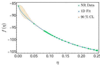
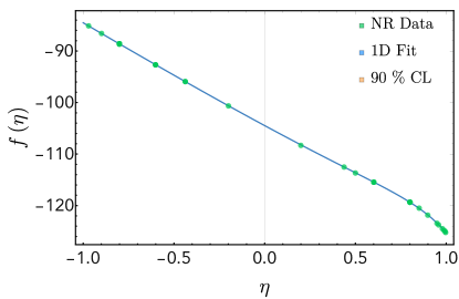
Figure 11: The 1D fits to the non-spinning and equal-mass, equal-spin subspaces. The blue curves show the 1D fits to the data and the orange shaded region denotes the 90% CL for the fit. The green points denote the NR and test-particle datasets. The equal-mass, equal-spin parameter space is extermely well understood. The non-spinning parameter space is densely covered up to $q\sim 10$ with only the non-spinning BAM simulation at $q=18$. Test-particle data can be used to pin the boundary at $q=1000$ but there is a clear degree of uncertainty in the intermediate region from $q>20$.

VIII.0.2 2D Fits

The two-dimensional fits to the $(\eta,\hat{S})$ subspace are constructed by combining both of the 1D subspace fits derived above. As discussed in Sec. IV.3, we generalize the $\hat{S}$-dependent fits by inserting a polynomial of order $J$ in $\eta$ for each coefficient in the 1D fit Jiménez-Forteza et al. (2017); Keitel et al. (2017). Here we opt to use a fourth order in $\eta$ expansion $(J=4)$ and kill the least constrained coefficients (i.e. p-values near unity) as determined by the non-linear model fit. In addition, we fix all coefficients on the denominator to avoid singularities. The constrained 2D fit $f(\eta,\hat{S})$ against the input data is shown in Fig. 12.

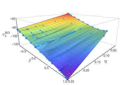
Figure 12: Fit $f(\eta,\hat{S})$ to the two-dimensional subspace $\{\eta,\hat{S}\}$. The blue points denote NR and test-particle data.

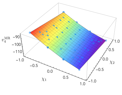
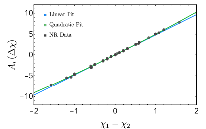
Figure 13: Example of the spin-difference behaviour at a mass ratio $q=3$. At such mass ratios the surface is very close to flat and the linear-in-spin difference term dominates.

VIII.0.3 Full 3D Fits

The final step in the procedure is to fit the unequal spin effects, parameterized by $\Delta\chi=\chi_{1}-\chi_{2}$, to the residual data, as discussed in Sec. IV.4. In Fig. 13, we show the unequal spin subspace for all $q=3$ NR data. As anticipated, the data is dominated by a linear-in-spin-difference terms with only weak evidence for higher order corrections. Fits are performed at all mass ratios for which we have sufficient data to constrain the ansatz. Note that the ansatz per-mass-ratio is used to inform the full 3D ansatz and as a consistency check. The 3D fit implemented in the model is constructed by fitting the constrained 2D ansatz plus the unequal spin terms to the full NR dataset. Here we demonstrate two approaches to constraining the unequal-spin fit. In the first approach, we restrict our analysis to the linear-in-spin-difference term $\Delta\chi$

$$\Delta v^{\rm{MR}}_{4}(\eta,\hat{S},\Delta\chi) =A_{1}(\eta)\Delta\chi.$$ (104)

In the second approach we use the full quadratic in unequal spin-correction ansataz

$$\Delta v^{\rm{MR}}_{4}(\eta,\hat{S},\Delta\chi) =f^{\rm{Lin}}(\eta)\Delta\chi+f^{\rm{Quad}}(\eta)\Delta\chi^{2}+f^{\rm{Mix}}(\eta)\hat{S}\,\Delta\chi.$$ (105)

Based on the symmetry arguments outlined in Jiménez-Forteza et al. (2017); Keitel et al. (2017) and Sec. IV.4, we adopt an ansatz for the linear in spin-difference term of the form

$$f^{\rm{Lin}}(\eta) =d_{10}\eta\left(1+d_{11}\right)\sqrt{1-4\eta}.$$ (106)

For the quadratic in spin-difference and mixed spin-difference ansätze, we adopt simpler fits of the form

$$f^{\rm{Quad}}(\eta) =d_{20}\eta,$$ (107)

$$f^{\rm{Mix}}(\eta) =d_{30}\eta\sqrt{1-4\eta}.$$ (108)

Whilst more complicated ansätze could be pursued, we typically find that the systematic errors in the NR data and strong correlations lead to poor constraints on the coefficients. As can be seen in the top two plots of Fig. 14, the shape and numerical value of the linear term is robust when adding different combinations of the unequal spin terms. Applying the fits to all data, we find

$$d_{10} =22.3632,$$ (109)

$$d_{11} =6.9794,$$ (110)

for the linear-only ansatz and

$$d_{10} =24.1579,$$ (111)

$$d_{11} =6.1330,$$ (112)

$$d_{20} =-0.4132,$$ (113)

$$d_{30} =6.1896$$ (114)

for the full ansatz. Though the data shows some evidence for quadratic-in-spin-difference corrections, third plot of Fig. 14, and mixed spin-difference terms, second plot of Fig. 14, systematic errors prevent a robust fit to the data. As such, for IMRPhenomXAS we opt to use the linear-only ansatz in the final 3D fit.

The full 3D fit to the data is

$$\Delta v^{\rm{MR}}_{4}(\eta,\hat{S},\Delta\chi) =\frac{a_{0}+a_{1}\eta+a_{2}\eta^{2}+a_{3}\eta^{3}+a_{4}\eta_{4}+a_{5}\eta_{6}}{1+a_{6}\eta}+\frac{1}{1+b_{6}\hat{S}}\Bigg{[}\hat{S}\left(c_{0}+c_{1}\eta+c_{2}\eta^{2}+c_{3}\eta^{3}+c_{4}\eta^{4}\right)$$ (115)

$$\quad+\hat{S}^{2}\left(d_{0}+d_{1}\eta+d_{2}\eta^{2}+d_{3}\eta^{3}+d_{4}\eta^{4}\right)+\hat{S}^{3}\left(e_{0}+e_{1}\eta+e_{2}\eta^{2}+e_{3}\eta^{3}+e_{4}\eta^{4}\right)$$

$$+\hat{S}^{4}\left(f_{0}+f_{1}\eta+f_{2}\eta^{2}+f_{3}\eta^{3}+f_{4}\eta^{4}\right)+\hat{S}^{5}\left(g_{0}+g_{1}\eta+g_{2}\eta^{2}+g_{3}\eta^{3}+g_{4}\eta^{4}\right)\Bigg{]}+h_{0}\left(1+h_{1}\eta\right)\sqrt{1-4\eta}\Delta\chi.$$

The coefficients $a_{i}$ are defined in Eqs. 101 and $b_{6}$ in Eq. 103. The additional coefficients are

$$c_{0} =-24.32, c_{1} =50.49$$

$$c_{2} =-68.32, c_{3} =0.0$$

$$c_{4} =784.98$$

$$d_{0} =26.62, d_{1} =-19.39$$

$$d_{2} =13.27, d_{3} =1092.51$$

$$d_{3} =2512.13,$$

$$e_{0} =2.80, e_{1} =11.23$$

$$e_{2} =-308.99, e_{3} =74.22$$

$$e_{4} =3103.82,$$

$$f_{0} =-1.68, f_{1} =-22.78$$

$$f_{2} =76.14, f_{3} =0.0$$

$$f_{4} =443.83,$$

$$g_{0} =-1.21, g_{1} =-71.28$$

$$g_{2} =525.24, g_{3} =0.0$$

$$g_{4} =3694.97,$$

$$h_{0} =22.36, h_{1} =6.98.$$

The full 3D fits for all coefficients required for IMRPhenomXAS are given in the supplementary material attached to this paper.

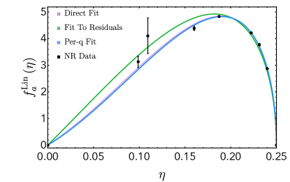
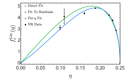
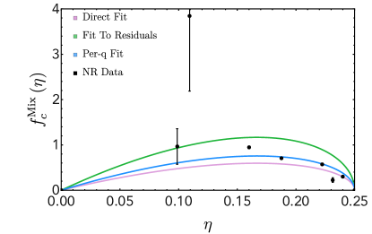
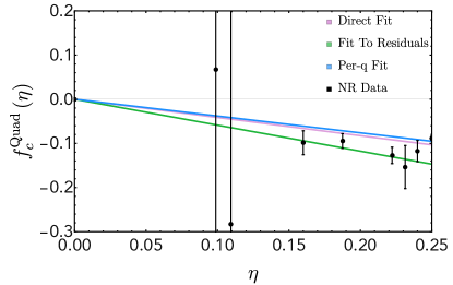
Figure 14: Fits to the unequal spin data. The first plot shows the linear-in-spin difference fit. The second plot shows the linear-in-spin difference contribution to the full unequal spin ansatz in Eq.40, $f^{\rm{Lin}}_{c}(\eta)\Delta\chi$ fit. The third plot the mixed-spin fit $f^{\rm{Mix}}_{c}(\eta)\,\hat{S}\,\Delta\chi$ and the final plot shows the quadratic in spin-difference fit $f^{\rm{Quad}}_{c}(\eta)\,\left(\Delta\chi\right)^{2}$. Whilst the linear-in-spin difference is relatively well captured, the second order unequal spin effects are less resolved with the coefficients for the fits becoming poorly constrained.

IX Model Validation

IX.1 Mismatches Against Hybrid Dataset

The agreement between two waveforms $h_{1}$ and $h_{2}$ can be quantified by the overlap, the noise-weighted inner product

$$\langle h_{1},h_{2}\rangle =4\ {\rm{Re}}\int^{f_{\rm{max}}}_{f_{\rm{min}}}\,\frac{\tilde{h}_{1}(f)\;\tilde{h}^{\ast}_{2}(f)}{S_{n}(f)}\,df.$$ (116)

The match is defined as the normalised ($\hat{h}=h/\sqrt{\langle h,h\rangle}$) inner product maximised over time and phase shifts

$$M(h_{1},h_{2})=\max\limits_{t_{0},\phi_{0}}\,\langle\hat{h}_{1},\hat{h}_{2}\rangle.$$ (117)

The mismatch is then defined as

$$\mathcal{M}(h_{1},h_{2})=1-M(h_{1},h_{2}).$$ (118)

In all matches presented here, we use the zero-detuned high-power (zdethp) PSD Aasi et al. (2015); Shoemaker . We use a low frequency cut-off of $20\rm{Hz}$ and an upper cut-off frequency of $8192\rm{Hz}$.

In order to assess the accuracy of our model, we compute the mismatch against all SXS hybrids produced for IMRPhenomXAS. As shown in Fig. 15, IMRPhenomXAS shows 1 to 2 orders of magnitude improvement over IMRPhenomD across the entire parameter space. Figure 16 shows mass-averaged mismatches for the performance of the four calibrated inspiral models discussed in Sec. VII.1. The inclusion of additional pseudo-PN coefficients demonstrates mild performance improvements, though not at a significantly appreciable level. In Fig. 17 we show mismatches for IMRPhenomXAS, IMRPhenomD and SEOBNRv4_ROM against NRHybSur3dq8 Varma et al. (2019) for mass ratios below 9.09 and dimensionless spin magnitudes up to 0.8.

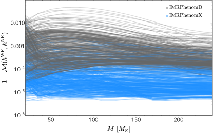
Figure 15: Mismatches for IMRPhenomXAS (blue) and IMRPhenomD (grey) against all SXS NR hybrids. We use the Advanced LIGO design sensitivity PSD and a lower frequency cutoff of $20$Hz. We see a dramatic decrease in the mismatch by $1$ to $2$ orders of magnitude across the parameter space.

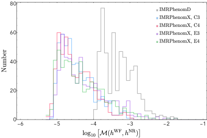
Figure 16: Mass averaged mismatches for IMRPhenomXAS and IMRPhenomD against all SXS NR hybrids. We use the Advanced LIGO design sensitivity PSD and a lower frequency cutoff of $20$Hz. We showcase four variants of IMRPhenomXAS corresponding to different inspiral models. The C denotes the canonical TaylorF2 baseline at 3.5PN and the E denotes the extension to $4$ and $4.5$PN discussed in the Appendix. The number, 3 or 4, denotes the number of pseudo-PN terms used in the model.

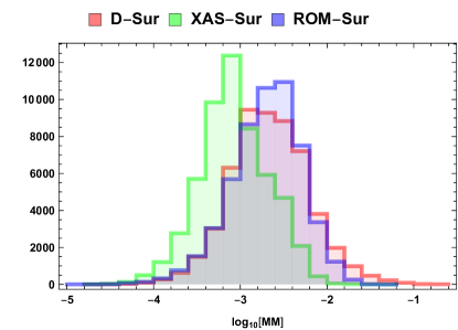
Figure 17: Mismatches ($\rm{MM}=\mathcal{M})$ for IMRPhenomXAS (green), IMRPhenomD (red) and SEOBNRv4 (blue) against NRHybSur3dq8, the NR hybrid surrogate valid up to a mass ratio $q=8$ and spins $\chi_{i}=\pm 0.8$. We compute the matches at random points in the parameter space, including points that fall between the calibration datasets used to construct IMRPhenomXAS. Here we clearly see that IMRPhenomXAS offers a significant improvement in performance in comparison to IMRPhenomD or SEOBNRv4.

IX.2 Time Domain Conversion

Although IMRPhenomXAS is expressed in terms of closed-form frequency domain expressions, the input calibration data and output from NR are time-domain function. It is therefore useful and illustrative to check the behaviour of the model when transformed from the frequency-domain back to the time-domain via an inverse Fourier transformation. In particular, the model should be a smooth function in both the frequency- and time-domain. Such comparisons are often useful as an additional consistency check on the physical accuracy of the model. In Fig. 18 we plot the time-domain reconstruction of IMRPhenomXAS against selected SXS or BAM waveforms at the boundary of the calibration region for NR. We find excellent agreement between IMRPhenomXAS and input NR data, even when considering near extremal spin configurations (first panel) as well as at large mass ratios and relatively large spins (last two panels). Note that we have optimized over a time and phase shift when aligning the waveforms. Such comparisons provide further evidence, in addition to the mismatches, that our end-to-end pipeline for hybridization, calibration and model reconstruction are faithfully reproducing the input data.

As in Khan et al. (2016), the frequency domain data is tapered and an optimal sampling rate chosen through the stationary phase approximation.

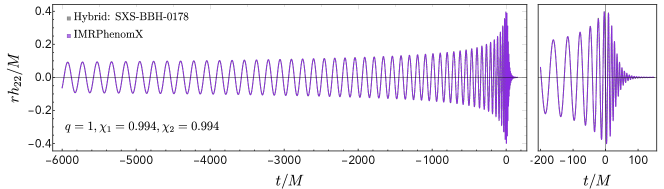
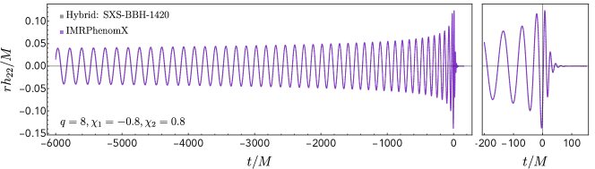
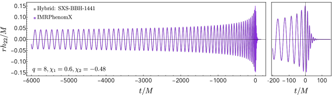
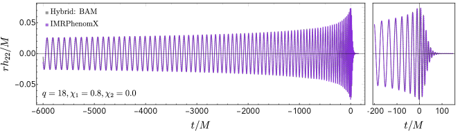
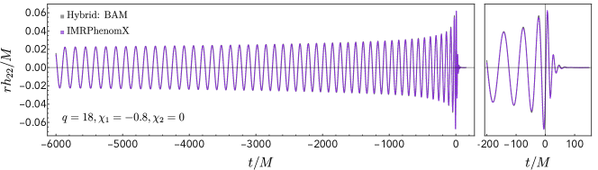
Figure 18: Time-domain IMRPhenomXAS waveforms (violet) and SEOBNRv4-NR hybrids (grey) for configurations at the edge of the calibration domain.

IX.3 Parameter Estimation

IX.3.1 GW150914

As an example of the application of IMRPhenomXAS to gravitational-wave data, we re-analyze GW150914 and demonstrate broad agreement between IMRPhenomXAS, IMRPhenomD and SEOBNRv4. We use coherent Bayesian inference methods to determine the posterior distribution $p(\vec{\theta}|\vec{d})$ for the parameters that characterize the binary. We use the nested sampling algorithm implemented in LALInference Veitch et al. (2015) and the public data from the Gravitational Wave Open Science Center (GWOSC) LIGO Scientific Collaboration, Virgo Collaboration (2019, 2018a, 2018b). Following Abbott et al. (2019), we marginalize over the frequency dependent spline calibration envelopes that characterize the uncertainty in the detector amplitude and strain. We analyze four seconds of strain data, with a lower cutoff frequency of 20Hz. Our choice of priors is as detailed in Section I of Appendix C in Abbott et al. (2019).

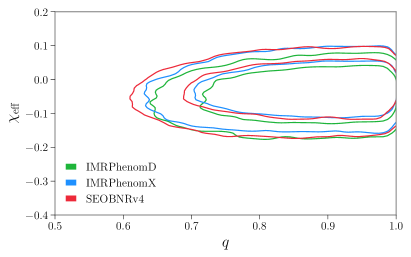
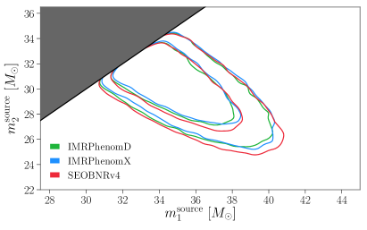
Figure 19: The top panel shows the $q-\chi_{\rm{eff}}$ 2D posteriors recovered by IMRPhenomXAS, IMRPhenomD and SEOBNRv4 when analysing GW150914. All models show excellent agreement. The bottom panel shows the recovered component masses in the source frame using the same waveform models. Note that the black line denotes the equal mass limit and we enforce $m_{1}>m_{2}$.

Figure 19 shows the posterior densities for the $\mathcal{M}-q$ and $q-\chi_{\rm{eff}}$ subspaces. The consistency between the three waveform models is in agreement with previous studies, demonstrating that systematic errors were below the statistical errors for this event Abbott et al. (2016b, 2017, c).

IX.3.2 NRHybSur3dq8

In the second example, we inject a NRHybSur3dq8 waveform into a HLV detector network assuming zero-noise and using the Advanced LIGO and Advanced VIRGO design sensitivity PSDs Barsotti et al. (2018); Aasi et al. (2015); Acernese et al. (2015). The injected waveform was taken to have a mass-ratio of $q=3$, chirp mass of $\mathcal{M}_{c}=20M_{\odot}$ and spins of $\chi_{1}=0.6$ and $\chi_{2}=-0.3$. The luminosity distance was $d_{L}=1\rm{Gpc}$ and the sky location, polarization and coalesence phase were arbitrarily chosen. Priors are again taken to be as detailed in Section I of Appendix C in Abbott et al. (2019). In Fig. 20, we highlight the reduced bias provided by IMRPhenomXAS over IMRPhenomD, demonstrating how the advances implemented in IMRPhenomXAS will help tighten and improve our constraints on the source properties of astrophysical black holes. A detailed study of waveform systematics and parameter biases is beyond the scope of this paper and will be presented in a forthcoming paper.

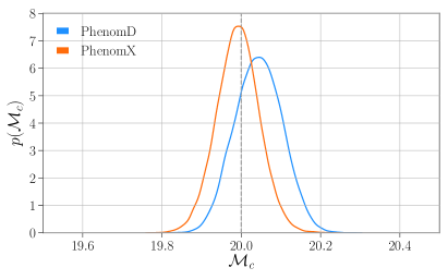
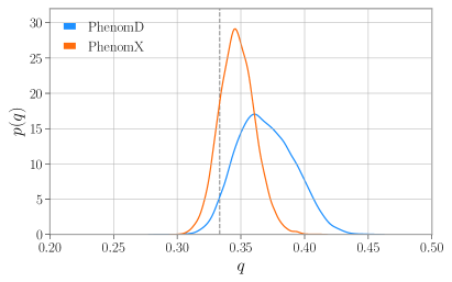
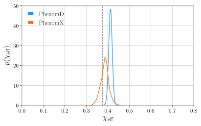
Figure 20: We show the 1D posterior distributions for the chirp mass $\mathcal{M}_{c}$, mass ratio $q$ and effective spin $\chi_{\rm{eff}}$ as recovered by IMRPhenomXAS and IMRPhenomD against an injected NRHybSur3dq8 waveform. The dashed line denotes the injected values. IMRPhenomXAS demonstrates excellent recovery of the injected parameters with significantly smaller biases and tighter posteriors than those exhibited by IMRPhenomD.

X Conclusions

In this paper we have presented a new model for the dominant $(2,\pm 2)$ spherical harmonics of the gravitational-wave signal from non-precessing, non-eccentric coalescing black holes. In gravitational wave data analysis, this model will most typically be used as part of a multi-mode waveform, where subdominant modes are included using the IMRPhenomXHM model, which we present in a companion paper García-Quirós et al. (2020a). Furthermore, a technique to accelerate waveform evaluation is available, which drastically reduces computational cost in particular for low masses (or low start frequencies), as discussed in a second companion paper García-Quirós et al. (2020b). Details of how to use the LALsuite The LIGO Scientific Collaboration (2015) implementation of the model are given in Appendix C of García-Quirós et al. (2020a).

In the following we summarize the main improvements of IMRPhenomXAS over IMRPhenomD. Several of the changes affect all of the three frequency regions:

• The number of NR waveforms the model is calibrated to has increased from 19 to 652. While IMRPhenomD was only calibrated to waveforms up to mass ratio 18. IMRPhenomXAS includes waveforms up to mass ratio 1000, which were computed in the in an appropriate test-particle limit as in Keitel et al. (2017), see Sec. III.

• IMRPhenomD modelled 2-dimensional parameter spaces of symmetric mass ratio and effective spin (choosing different effective spins in different frequency regimes as appropriate). IMRPhenomXAS models the complete 3-dimensional parameter space without effective spin approximations.

• Ad-hoc parameter space fits have been replaced by a systematic procedure designed to avoid both underfitting and overfitting Jiménez-Forteza et al. (2017); Keitel et al. (2017), which proceeds by hierarchically treating sub-spaces like the non-spinning, or equal-spin systems.

• A dramatic improvement in the accuracy of IMRPhenomXAS over IMRPhenomD. Notably, we find 1 to 2 orders of magnitude improvement in the mismatches against the SEOBNRv4-NR hybrids across the parameter space.

• IMRPhenomXAS incorporates physically motivated transition regions, with the key frequencies obeying a natural hierarchy.

• The improvements mentioned above also facilitated a more systematic study regarding the optimal parameterization of a given waveform model, in particular concerning the use of coefficients of basis functions versus the use of collocation points, see Sec. IV.1.

• Finally, the implementation in the LAL software library for gravitational wave data analysis The LIGO Scientific Collaboration (2015) has been modularized, to allow independent updates for the inspiral, intermediate and ringdown regions of teh phase or amplitude models.

Our description of the inspiral region has improved due to a lower cutoff frequency of 74% of the IMRPhenomD value for the inspiral calibration, which corresponds to approximately doubling the length of the waveform in the time domain. In addition, the transition frequency from inspiral to the intermediate region is now carefully chosen as a function of parameter space, instead of set to a fixed frequency, as discussed in Sec. V, and different post-Newtonian orders of the underlying TaylorF2 approximant have been compared. Modelling of the intermediate frequency region also greatly benefits from our careful choice of transition frequencies. In addition we have added further degrees of freedom for more accurate fits.

Finally, several changes affect mostly the ringdown, or more generally the highest frequencies:

• Hybrid waveforms have been built from the Newman-Penrose scalar $\psi_{4}$ (see e.g. Husa et al. (2020)) instead of from the strain, which results in a significantly cleaner ringdown waveform.

• The time resolution for hybrid waveforms has been increased from $M\Delta t=1$ to $M\Delta t=0.5$, which benefits high spin cases with high ringdown frequencies.

• The fits for final spin and final mass, which are required for computing the complex ringdown frequency, have been changed from using the 2-dimensional effective spin fits of Khan et al. (2016) to modelling the full 3-dimensional parameter space dependency, which eliminates the necessity to model the discrepancy between the value from ringdown frequency according to the fits with an extra parameter.

An important challenge for the future is to improve the modelling of extreme mass ratios, and to study the transition between comparable and extreme mass ratios. An important element here will be to extend the catalogue of accurate and sufficiently long numerical relativity waveforms beyond mass ratio 18.

Appendix A TaylorF2

Here we incorporate non-spinning corrections to $3.5$PN order, spin-orbit corrections to $3.5$PN, spin-orbit tail corrections to $4$PN, quadratic-in-spin corrections to $3$PN and the cubic-in-spin $3.5$PN corrections.

A.1 Amplitude

The inspiral amplitude is based on the re-expanded PN amplitude TaylorF2

$$A_{\rm{PN}}(f;\Xi)=A_{0}\displaystyle\sum^{6}_{i=0}\,\mathcal{A}_{i}\,\left(\pi f\right)^{i/3},$$ (119)

where $\Xi=\{\eta,\chi_{1},\chi_{2}\}$. The expansion coefficients are given by

$$\mathcal{A}_{0}=1,$$ (120)

$$\mathcal{A}_{1}=0,$$ (121)

$$\mathcal{A}_{2}=-\frac{323}{224}+\frac{451\eta}{168}.$$ (122)

$$\mathcal{A}_{3}={\chi_{1}}\left(\frac{27\delta}{16}-\frac{11\eta}{12}+\frac{27}{16}\right)+{\chi_{2}}\left(-\frac{27\delta}{16}-\frac{11\eta}{12}+\frac{27}{16}\right)$$ (123)

$$\mathcal{A}_{4} ={\chi_{1}}^{2}\left(-\frac{81\delta}{64}+\frac{81\eta}{32}-\frac{81}{64}\right)$$ (124)

$$\quad\;+{\chi_{2}}^{2}\left(\frac{81\delta}{64}+\frac{81\eta}{32}-\frac{81}{64}\right)$$

$$\quad\;+\left(\frac{105271}{24192}\eta^{2}-\frac{1975055}{338688}\eta-\frac{27312085}{8128512}\right)$$

$$\quad\;-\frac{47}{16}\,\eta\,{\chi_{1}}\,{\chi_{2}}$$

$$\mathcal{A}_{5} ={\chi_{1}}^{3}\left(\delta\left(\frac{3}{16}-\frac{3\eta}{16}\right)-\frac{9\eta}{16}+\frac{3}{16}\right)+$$ (125)

$$\quad\,{\chi_{1}}\left(\delta\left(\frac{287213}{32256}-\frac{2083\eta}{8064}\right)-\frac{2227\eta^{2}}{2016}-\frac{15569\eta}{1344}+\frac{287213}{32256}\right)+$$

$$\quad\,{\chi_{2}}^{3}\left(\delta\left(\frac{3\eta}{16}-\frac{3}{16}\right)-\frac{9\eta}{16}+\frac{3}{16}\right)+$$

$$\quad\,{\chi_{2}}\left(\delta\left(\frac{2083\eta}{8064}-\frac{287213}{32256}\right)-\frac{2227\eta^{2}}{2016}-\frac{15569\eta}{1344}+\frac{287213}{32256}\right)$$

$$\quad\,-\frac{85\pi}{64}+\frac{85\pi\eta}{16}$$

$$\mathcal{A}_{6} ={\chi_{1}}\left(-\frac{17\pi\delta}{12}+\left(-\frac{133249\eta^{2}}{8064}-\frac{319321\eta}{32256}\right){\chi_{2}}+\frac{5\pi\eta}{3}-\frac{17\pi}{12}\right)$$ (126)

$$\quad\,+{\chi_{1}}^{2}\left(\delta\left(-\frac{141359\eta}{32256}-\frac{49039}{14336}\right)+\frac{163199\eta^{2}}{16128}+\frac{158633\eta}{64512}-\frac{49039}{14336}\right)$$

$$\quad\,+{\chi_{2}}^{2}\left(\delta\left(\frac{141359\eta}{32256}+\frac{49039}{14336}\right)+\frac{163199\eta^{2}}{16128}+\frac{158633\eta}{64512}-\frac{49039}{14336}\right)+{\chi_{2}}\left(\frac{17\pi\delta}{12}+\frac{5\pi\eta}{3}-\frac{17\pi}{12}\right)$$

$$\quad\,-\frac{177520268561}{8583708672}+\left(\frac{545384828789}{5007163392}-\frac{205\pi^{2}}{48}\right)\eta-\frac{3248849057\eta^{2}}{178827264}+\frac{34473079\eta^{3}}{6386688}$$

A.2 Phase

The underlying frequency-domain phasing model in IMRPhenomX is based on the TaylorF2 post-Newtonian approximant constructed via the application of the stationary phase approximation (SPA). For quasi-circular, non-precessing binaries, the input ingredients are the center-of-mass energy $E$ and the energy flux $F$. The canonical TaylorF2 approximant used in IMRPhenomX implements recent tail-induced spin-orbit terms at 4PN, cubic-in-spin corrections at 3.5PN and quadratic-in-spin corrections at 3PN. Schematically, the energy can be written as

$$E =-\frac{\eta}{2}x\left[E_{\rm{NS}}+x^{3/2}E_{\rm{SO}}+x^{2}E_{\rm{SS}}+x^{7/2}E_{\rm{SSS}}\right]$$ (127)

where $E_{\rm{NS}}$, $E_{\rm{SO}}$, $E_{\rm{SS}}$ and $E_{\rm{SSS}}$ the non-spinning, spin-orbit, quadratic-in-spin and cubic-in-spin corrections to the energy. Although the non-spinning contributions are currently known to 4PN, the baseline model presented here restricts the non-spinning contributions to 3PN. The spin-orbit terms begin at 1.5PN order are currently known to 3.5PN Marsat (2015); Bohé et al. (2015). The quadratic-in-spin corrections are known at next-to-leading order, coresponding to 3PN Bohé et al. (2015). The cubic-in-spin terms are currently known to leading order and enter the energy and flux at 3.5PN Marsat (2015).

Similarly, the flux can be written as

$$\mathcal{F} =\frac{32}{5}\eta x^{5}\left[\mathcal{F}_{\rm{NS}}+x^{3/2}\mathcal{F}_{\rm{SO}}+x^{2}\mathcal{F}_{\rm{SS}}+x^{7/2}\mathcal{F}_{\rm{SSS}}\right]$$ (128)

where $\mathcal{F}_{\rm{NS}}$, $\mathcal{F}_{\rm{SO}}$, $\mathcal{F}_{\rm{SS}}$ and $\mathcal{F}_{\rm{SSS}}$ denote the non-spinning, spin-orbit, quadratic-in-spin and cubic-in-spin corrections to post-Newtonian energy flux.

The frequency-domain phase from the TaylorF2 terms is given by

$$\varphi_{\rm{TF}2}\,(f;\Xi) =2\pi ft_{c}-\varphi_{c}-\frac{\pi}{4}$$ (129)

$$\qquad+\frac{3}{128\eta}\left(\pi fM\right)^{-5/3}\,\displaystyle\sum^{7}_{i=0}\,\varphi_{i}\left(\Xi\right)\,\left(\pi fM\right)^{i/3}.$$

In IMRPhenomD, the TaylorF2 baseline was based on non-spinning corrections to 3.5PN, linear spin-orbit corrections to 3.5PN and quadratic spin corrections to 2PN. In addition, upon re-expanding the PN energy and flux in deriving the TaylorF2 phase, all quadratic and higher spin corrections beyond 2PN were implicitly dropped. The coefficients used in IMRPhenomXAS incorporate relative 1PN quadratic-in-spin corrections, the leading-order cubic-in-spin corrections and a tail-induced SO term entering at 4PN, $\varphi_{8}$. The coefficients detailed below define the canonical TaylorF2 model discussed in Sec. VII.1

$$\varphi_{0} =1$$ (130)

$$\varphi_{1} =0$$ (131)

$$\varphi_{2} =\frac{55\eta}{9}+\frac{3715}{756}$$ (132)

$$\varphi_{3} =\frac{113\delta\chi_{a}}{3}+\left(\frac{113}{3}-\frac{76\eta}{3}\right)\chi_{s}-16\pi$$ (133)

$$\varphi_{4} =-\frac{405}{4}\delta\,\chi_{a}\,\chi_{s}+\left(200\eta-\frac{405}{8}\right)\chi_{a}^{2}+\left(\frac{5\eta}{2}-\frac{405}{8}\right)\chi_{s}^{2}+\frac{15293365}{508032}+\frac{27145}{504}\eta+\frac{3085}{72}\eta^{2}$$ (134)

$$\varphi_{5} =\chi_{a}\left(-\frac{140\delta\eta}{9}-\frac{732985\delta}{2268}+\left(-\frac{140\delta\eta}{9}-\frac{732985\delta}{2268}\right)\log(\pi f)\right)$$ (135)

$$\qquad+\chi_{s}\left(\left(\frac{340\eta^{2}}{9}+\frac{24260\eta}{81}-\frac{732985}{2268}\right)\log(\pi f)+\frac{340\eta^{2}}{9}+\frac{24260\eta}{81}-\frac{732985}{2268}\right)$$

$$\qquad+\left(\frac{38645\pi}{756}-\frac{65\pi\eta}{9}\right)\log(\pi f)-\frac{65\pi}{9}\eta+\frac{38645\pi}{756}$$

$$\varphi_{6} =\chi_{s}\left(\chi_{a}\left(\frac{75515\delta}{144}-\frac{8225\delta\eta}{18}\right)-520\pi\eta+\frac{2270\pi}{3}\right)+\frac{2270\pi\delta\chi_{a}}{3}-\frac{6848}{63}\log(\pi f)-\frac{127825\eta^{3}}{1296}$$ (136)

$$\qquad+\left(-480\eta^{2}-\frac{263245\eta}{252}+\frac{75515}{288}\right)\chi_{a}^{2}+\left(\frac{1255\eta^{2}}{9}-\frac{232415\eta}{504}+\frac{75515}{288}\right)\chi_{s}^{2}$$

$$\qquad+\frac{76055\eta^{2}}{1728}+\frac{2255\pi^{2}\eta}{12}-\frac{15737765635\eta}{3048192}-\frac{640\pi^{2}}{3}-\frac{6848\gamma_{E}}{21}+\frac{11583231236531}{4694215680}-\frac{13696\log(2)}{21}$$

$$\varphi_{7} =\chi_{a}\left(-\frac{1985\delta\eta^{2}}{48}+\frac{26804935\delta\eta}{6048}-\frac{25150083775\delta}{3048192}\right)$$ (137)

$$\qquad+\chi_{s}\left(-1140\pi\delta\chi_{a}+\frac{5345\eta^{3}}{36}+\left(80\eta^{2}-7270\eta+\frac{14585}{8}\right)\chi_{a}^{2}-\frac{1042165\eta^{2}}{3024}+\frac{10566655595\eta}{762048}-\frac{25150083775}{3048192}\right)$$

$$\qquad+\chi_{a}^{3}\left(\frac{14585\delta}{24}-2380\delta\eta\right)+\chi_{s}^{2}\left(\text{$\chi$a}\left(\frac{14585\delta}{8}-\frac{215\delta\eta}{2}\right)+40\pi\eta-570\pi\right)+\left(\frac{100\eta^{2}}{3}-\frac{475\eta}{6}+\frac{14585}{24}\right)\chi_{s}^{3}$$

$$\qquad-\frac{74045\pi\eta^{2}}{756}+(2240\pi\eta-570\pi)\chi_{a}^{2}+\frac{378515\pi\eta}{1512}+\frac{77096675\pi}{254016}$$

$$\varphi_{8} =\pi\Bigg{[}\chi_{a}\left(-\frac{99185}{252}\delta\eta+\frac{233915\delta}{168}+\left(\frac{99185\delta\eta}{252}-\frac{233915\delta}{168}\right)\log(\pi f)\right)$$ (138)

$$\qquad+\chi_{s}\left(\left(-\frac{19655\eta^{2}}{189}+\frac{3970375\eta}{2268}-\frac{233915}{168}\right)\log(\pi f)+\frac{19655\eta^{2}}{189}-\frac{3970375\eta}{2268}+\frac{233915}{168}\right)\Bigg{]}.$$

A.3 Extending Results to $4.5$PN

An implicit and powerful feature of the current generation of phenomenological waveform models is the implicit modularity. By separating the waveform into three key regimes we are free to recalibrate or improve aspects of the waveform model in reaction to the latest developments in the literature. A worked example of this would be the extension of the results to include the latest 4PN and 4.5PN results in the literature. For the non-spinning sector, the equations of motion for compact binaries has been derived to $4$PN Damour et al. (2014); Jaranowski and Schäfer (2015); Damour and Jaranowski (2017); Bernard et al. (2016); Marchand et al. (2018) leading to an additional non-spinning term of the form

$$E^{\rm{4PN}} =x^{4}\Bigg{[}\frac{77}{31104}\eta^{4}+\frac{301}{1728}\eta^{3}+\left(\frac{3157\pi^{2}}{576}-\frac{498449}{3456}\right)\eta^{2}+\eta\left(\frac{448}{15}\log(16x)+\frac{9037\pi^{2}}{1536}+\frac{896}{15}\gamma_{E}-\frac{123671}{5760}\right)-\frac{3969}{128}\Bigg{]}.$$ (139)

As well as the $4$PN derivation above, higher non-linear tail effects associated to quartic non-linear interactions have recently been derived from first principles in the MPM formalism Marchand et al. (2016) as well as an independent derivation from the PN re-expansion of the factorized and resummed EOB fluxes Messina et al. (2018). Such interactions lead to a $4.5$PN contribution to the flux

$$\mathcal{F}^{\rm{4.5PN}}_{\rm{Tail}} =\pi\,x^{9/2}\left[-\frac{3719141\eta^{3}}{38016}-\frac{133112905\eta^{2}}{290304}+\left(\frac{2062241}{22176}+\frac{41\pi^{2}}{12}\right)\eta-\frac{3424}{105}\log(16x)-\frac{6848\gamma}{105}+\frac{265978667519}{745113600}\right].$$ (140)

Another interesting contribution derived from the PN re-expansion of the EOB fluxes is the identification of a leading-order tail-induced spin-spin term in the flux Messina et al. (2018)

$$\mathcal{F}^{\rm{3.5PN}}_{\rm{LO-SS,Tail}} =\pi\,x^{7/2}\Bigg{[}\left(8\delta^{2}+\frac{1}{8}\right)\chi_{a}^{2}$$ (141)

$$\qquad\qquad\qquad+\left(\frac{\delta^{2}}{8}+8\right)\chi_{s}^{2}+\frac{65}{4}\delta\,\chi_{a}\,\chi_{s}\Bigg{]},$$

which coincides with the known test-particle limit Tagoshi et al. (1996). Adding these terms to the PN flux and energy, we find the following higher order contributions to the PN phasing

$$\varphi_{7}^{N} =-\pi x^{7/2}\left[-325\,\delta\,\chi_{a}\,\chi_{s}+\left(640\eta-\frac{325}{2}\right)\,\chi_{a}^{2}+\left(10\eta-\frac{325}{2}\right)\,\chi_{s}^{2}\right]$$ (142)

$$\varphi_{9}^{N} =\pi x^{9/2}\Bigg{[}\frac{10323755}{199584}\eta^{3}+\frac{45293335}{127008}\eta^{2}+\left(-\frac{1492917260735}{134120448}+\frac{2255\pi^{2}}{6}\right)\eta$$ (143)

$$\qquad\qquad-\frac{6848\log(x)}{21}-\frac{640\pi^{2}}{3}-\frac{13696}{21}\gamma_{E}+\frac{105344279473163}{18776862720}-\frac{27392\log(2)}{21}\Bigg{]},$$

in agreement with Messina et al. (2018) and Nagar et al. (2019c). A somewhat more vexing task is how to incorporate, in a fully-consistent way, the incomplete knowledge at $4$PN. One possible approach, as taken in Messina et al. (2018), is to construct an approximant that depends on as of yet unknown analytical coefficients $c_{N}$, allowing the incomplete $4$ and $4.5$PN terms to be included in a fully-consistent way, complete with $\eta$ dependence. Here, however, we choose to drop the unknown analytical information and instead absorb these into the pseudo-PN calibration. In practice, we do not find any significant difference between the canonical TaylorF2 approximant used and the higher order PN expressions given here after the pseudo-PN calibration is taken into account. The extended TaylorF2 approximant discussed in Sec. VII.1 uses the coefficients detailed in Eqs. 130 to A.2 plus the additional terms in Eqs. 142 and 143.

Appendix B Stationary Phase Approximation

Here we overview the stationary phase approximation (SPA) applied to a time domain signal Finn and Chernoff (1993); Cutler and Flanagan (1994); Droz et al. (1999)

$$h_{\ell m}(t)=A_{\ell m}(t)\;e^{-i\;m\;\varphi(t)}.$$

The orbital phase $\varphi$ is related to the orbital frequency by $\omega=\dot{\varphi}$. The SPA approximation is formally valid if the following criteria are met Cutler and Flanagan (1994); Finn and Chernoff (1993); Marsat and Baker (2018)

$$\left|\frac{\dot{A}/A}{\omega}\right|\ll 1,\quad\left|\frac{\dot{\omega}}{\omega^{2}}\right|\ll 1,\quad\left|\frac{(\dot{A}/A)^{2}}{\dot{\omega}}\right|\ll 1.$$

The SPA approximation works as the Fourier transform of a signal is highly oscillatory and unless there are strong cancellations between the orbital phase $\varphi(t)$ and the $2\pi ft$ term, the Fourier transform will have support that is roughly centered on the point of stationary phase. This enables us to define a time as a function of the frequency

$$m\;\omega\,(t_{f}) =2\pi f,$$

where $t_{f}$ is strictly only valid in the SPA regime. Assuming a monotonically increasing orbital phase, such that $\omega>0$ and $\dot{\omega}>0$, then we can expand the signal about the SPA time

$$\tilde{h}_{\rm SPA}(f)\simeq A_{\ell m}(t_{f})\;e^{2\pi ift_{f}-mi\varphi\,(t_{f})}\;\int e^{-i\,(t-t_{f})^{2}\,m\,\dot{\omega}\,(t_{f})\,/2}dt$$

Noting that $|(\dot{A}/A)^{2}/\dot{\omega}|\ll 1$, we can treat the amplitude as being approximately constant. Performing the Gaussian integration, we find

$$\tilde{h}{\ell m}(f) \simeq A_{\ell m}(f)\;e^{-i\Psi_{\ell m}(f)},$$

$$A_{\ell m}(f) \simeq A_{\ell m}(t_{f})\;\sqrt{\frac{2\pi}{m\dot{\omega}(t_{f})} },$$

$$\Psi_{\ell m}(f) \simeq m\;\varphi(t_{f})-2\pi ft_{f}+\frac{\pi}{4},$$

where we have made use of the standard integral $\int^{\infty}_{-\infty}dx\;e^{-ix^{2}}=\sqrt{\pi}e^{-i\pi/4}$. This can now be expressed in terms of the TaylorF2 phase $\varphi_{\ell m}^{\rm TF2}$ and a phase shift $\varphi_{0,\ell m}$

$$\Psi_{\ell m}(f) \simeq-2\pi ft_{0}+\frac{\pi}{4}+\varphi_{0,\ell m}+\varphi_{\ell m}^{\rm TF2}(f)$$

where

$$\varphi_{0,\ell m}=\frac{m}{2}\;\varphi_{0,22}+\varphi_{\ell m}^{\rm Amp},$$

and

$$\varphi_{\ell m}^{\rm TF2}(f) =\frac{m}{2}\varphi_{22}^{\rm TF2}\left(\frac{2f}{m}\right).$$ (144)

The term $\varphi^{\rm Amp}_{\ell m}$ corresponds to phase corrections arising from the complex PN amplitudes and $\varphi_{0,\ell,m}$ a gauge freedom associated to phase shifts. Collecting this all together, we can write the SPA of the time domain mode as

$$\tilde{h}_{\ell m}(f) =A_{\ell m}(t_{f})\;\sqrt{ \frac{2\pi}{m\dot{\omega}}}\;e^{i\left[2\pi ft_{f}-m\varphi(t_{f})-\pi/4\right]}.$$ (145)

References

- Husa et al. (2016) S. Husa, S. Khan, M. Hannam, M. Pürrer, F. Ohme, X. Jiménez Forteza, and A. Bohé, Phys. Rev. D93, 044006 (2016), arXiv:1508.07250 [gr-qc] .
- Khan et al. (2016) S. Khan, S. Husa, M. Hannam, F. Ohme, M. Pürrer, X. Jiménez Forteza, and A. Bohé, Phys. Rev. D93, 044007 (2016), arXiv:1508.07253 [gr-qc] .
- Hannam et al. (2014) M. Hannam, P. Schmidt, A. Bohé, L. Haegel, S. Husa, et al., Phys.Rev.Lett. 113, 151101 (2014), arXiv:1308.3271 [gr-qc] .
- London et al. (2018) L. London, S. Khan, E. Fauchon-Jones, C. García, M. Hannam, S. Husa, X. Jiménez-Forteza, C. Kalaghatgi, F. Ohme, and F. Pannarale, Phys. Rev. Lett. 120, 161102 (2018), arXiv:1708.00404 [gr-qc] .
- García-Quirós et al. (2020a) C. García-Quirós, M. Colleoni, S. Husa, H. Estellés, G. Pratten, A. Ramos-Buades, M. Mateu-Lucena, and R. Jaume, (2020a), arXiv:2001.10914 [gr-qc] .
- Pratten et al. (2019) G. Pratten, C. García Quirós, M. Colleoni, A. Ramos-Buades, , H. Estellés, M. Mateu, R. Jaume, and S. Husa, (2019).
- Usman et al. (2016) S. A. Usman et al., Class. Quant. Grav. 33, 215004 (2016), arXiv:1508.02357 [gr-qc] .
- Sachdev et al. (2019) S. Sachdev et al., (2019), arXiv:1901.08580 [gr-qc] .
- Veitch et al. (2015) J. Veitch et al., Phys. Rev. D91, 042003 (2015), arXiv:1409.7215 [gr-qc] .
- Ashton et al. (2019) G. Ashton et al., Astrophys. J. Suppl. 241, 27 (2019), arXiv:1811.02042 [astro-ph.IM] .
- Abbott et al. (2016a) B. P. Abbott et al. (LIGO Scientific, Virgo), Phys. Rev. Lett. 116, 061102 (2016a), arXiv:1602.03837 [gr-qc] .
- Abbott et al. (2016b) B. P. Abbott et al. (LIGO Scientific, Virgo), Phys. Rev. Lett. 116, 241102 (2016b), arXiv:1602.03840 [gr-qc] .
- Abbott et al. (2019) B. P. Abbott et al. (LIGO Scientific, Virgo), Phys. Rev. X9, 031040 (2019), arXiv:1811.12907 [astro-ph.HE] .
- Abbott et al. (2017) B. P. Abbott et al. (LIGO Scientific, Virgo), Class. Quant. Grav. 34, 104002 (2017), arXiv:1611.07531 [gr-qc] .
- Pan et al. (2014) Y. Pan, A. Buonanno, A. Taracchini, L. E. Kidder, A. H. Mroué, H. P. Pfeiffer, M. A. Scheel, and B. Szilágyi, Phys. Rev. D89, 084006 (2014), arXiv:1307.6232 [gr-qc] .
- Taracchini et al. (2014) A. Taracchini et al., Phys. Rev. D89, 061502 (2014), arXiv:1311.2544 [gr-qc] .
- Pürrer (2016) M. Pürrer, Phys. Rev. D93, 064041 (2016), arXiv:1512.02248 [gr-qc] .
- Bohé et al. (2017) A. Bohé et al., Phys. Rev. D95, 044028 (2017), arXiv:1611.03703 [gr-qc] .
- Babak et al. (2017) S. Babak, A. Taracchini, and A. Buonanno, Phys. Rev. D95, 024010 (2017), arXiv:1607.05661 [gr-qc] .
- García-Quirós et al. (2020b) C. García-Quirós, S. Husa, M. Mateu-Lucena, and A. Borchers, (2020b), arXiv:2001.10897 [gr-qc] .
- Vinciguerra et al. (2017) S. Vinciguerra, J. Veitch, and I. Mandel, Class. Quant. Grav. 34, 115006 (2017), arXiv:1703.02062 [gr-qc] .
- Khan et al. (2019) S. Khan, K. Chatziioannou, M. Hannam, and F. Ohme, Phys. Rev. D100, 024059 (2019), arXiv:1809.10113 [gr-qc] .
- Ajith et al. (2011) P. Ajith et al., Phys. Rev. Lett. 106, 241101 (2011), arXiv:0909.2867 [gr-qc] .
- Santamaria et al. (2010) L. Santamaria et al., Phys. Rev. D82, 064016 (2010), arXiv:1005.3306 [gr-qc] .
- Kumar et al. (2016) P. Kumar, T. Chu, H. Fong, H. P. Pfeiffer, M. Boyle, D. A. Hemberger, L. E. Kidder, M. A. Scheel, and B. Szilagyi, Phys. Rev. D93, 104050 (2016), arXiv:1601.05396 [gr-qc] .
- Jiménez-Forteza et al. (2017) X. Jiménez-Forteza, D. Keitel, S. Husa, M. Hannam, S. Khan, and M. Pürrer, Phys. Rev. D95, 064024 (2017), arXiv:1611.00332 [gr-qc] .
- Harms et al. (2014) E. Harms, S. Bernuzzi, A. Nagar, and A. Zenginoglu, Class. Quant. Grav. 31, 245004 (2014), arXiv:1406.5983 [gr-qc] .
- Harms et al. (2016a) E. Harms, G. Lukes-Gerakopoulos, S. Bernuzzi, and A. Nagar, Phys. Rev. D93, 044015 (2016a), [Addendum: Phys. Rev.D100,no.12,129901(2019)], arXiv:1510.05548 [gr-qc] .
- Harms et al. (2016b) E. Harms, G. Lukes-Gerakopoulos, S. Bernuzzi, and A. Nagar, Phys. Rev. D94, 104010 (2016b), arXiv:1609.00356 [gr-qc] .
- Husa et al. (2020) S. Husa, M. Colleoni, H. Estellés, G. Q. Cecilio, A. Ramos-Buades, G. Pratten, R. Jaume, X. Jimenez-Forteza, and D. Keitel, (2020).
- Wiaux et al. (2007) Y. Wiaux, L. Jacques, and P. Vandergheynst, J. Comput. Phys. 226, 2359 (2007), arXiv:astro-ph/0508514 [astro-ph] .
- The LIGO Scientific Collaboration (2015) The LIGO Scientific Collaboration, “LALSuite: LSC Algorithm Library Suite,” https://www.lsc-group.phys.uwm.edu/daswg/projects/lalsuite.html (2015).
- Finn and Chernoff (1993) L. S. Finn and D. F. Chernoff, Phys. Rev. D47, 2198 (1993), arXiv:gr-qc/9301003 [gr-qc] .
- Cutler and Flanagan (1994) C. Cutler and E. E. Flanagan, Phys. Rev. D49, 2658 (1994), arXiv:gr-qc/9402014 [gr-qc] .
- Damour et al. (2000) T. Damour, B. R. Iyer, and B. S. Sathyaprakash, Phys. Rev. D62, 084036 (2000), arXiv:gr-qc/0001023 [gr-qc] .
- Calderón Bustillo et al. (2015) J. Calderón Bustillo, A. Bohé, S. Husa, A. M. Sintes, M. Hannam, and M. Pürrer, (2015), arXiv:1501.00918 [gr-qc] .
- Blanchet (2014) L. Blanchet, Living Reviews in Relativity 17 (2014), 10.12942/lrr-2014-2.
- Damour (2001) T. Damour, Phys. Rev. D64, 124013 (2001), arXiv:gr-qc/0103018 [gr-qc] .
- Damour et al. (2002) T. Damour, B. R. Iyer, and B. S. Sathyaprakash, Phys. Rev. D66, 027502 (2002), arXiv:gr-qc/0207021 [gr-qc] .
- Arun et al. (2005) K. G. Arun, B. R. Iyer, B. S. Sathyaprakash, and P. A. Sundararajan, Phys. Rev. D71, 084008 (2005), [Erratum: Phys. Rev.D72,069903(2005)], arXiv:gr-qc/0411146 [gr-qc] .
- Buonanno et al. (2009) A. Buonanno, B. Iyer, E. Ochsner, Y. Pan, and B. S. Sathyaprakash, Phys. Rev. D80, 084043 (2009), arXiv:0907.0700 [gr-qc] .
- Kokkotas and Schmidt (1999) K. Kokkotas and B. Schmidt, Living Reviews in Relativity 2 (1999).
- Cabero et al. (2017) M. Cabero, A. B. Nielsen, A. P. Lundgren, and C. D. Capano, Phys. Rev. D95, 064016 (2017), arXiv:1602.03134 [gr-qc] .
- Trefethen, Lloyd N. (1996) Trefethen, Lloyd N., Finite Difference and Spectral Methods for Ordinary and Partial Differential Equations (1996).
- Luna and Sintes (2006) M. Luna and A. M. Sintes, Class. Quant. Grav. 23, 3763 (2006), arXiv:gr-qc/0601072 [gr-qc] .
- Kumar Mehta et al. (2019) A. Kumar Mehta, P. Tiwari, N. K. Johnson-McDaniel, C. K. Mishra, V. Varma, and P. Ajith, Phys. Rev. D100, 024032 (2019), arXiv:1902.02731 [gr-qc] .
- Ajith et al. (2007) P. Ajith et al., Gravitational wave data analysis. Proceedings: 11th Workshop, GWDAW-11, Potsdam, Germany, Dec 18-21, 2006, Class. Quant. Grav. 24, S689 (2007), arXiv:0704.3764 [gr-qc] .
- Ajith et al. (2008) P. Ajith et al., Phys. Rev. D77, 104017 (2008), [Erratum: Phys. Rev.D79,129901(2009)], arXiv:0710.2335 [gr-qc] .
- McWilliams (2019) S. T. McWilliams, Phys. Rev. Lett. 122, 191102 (2019), arXiv:1810.00040 [gr-qc] .
- Buonanno and Damour (1999a) A. Buonanno and T. Damour, Phys. Rev. D59, 084006 (1999a), arXiv:gr-qc/9811091 [gr-qc] .
- Buonanno and Damour (1999b) A. Buonanno and T. Damour, Phys. Rev. D 59 (1999b), 10.1103/physrevd.59.084006.
- Nagar et al. (2018) A. Nagar et al., Phys. Rev. D98, 104052 (2018), arXiv:1806.01772 [gr-qc] .
- Ossokine et al. (2013) S. Ossokine, L. E. Kidder, and H. P. Pfeiffer, Phys.Rev. D88, 084031 (2013), arXiv:1304.3067 [gr-qc] .
- Hemberger et al. (2013) D. A. Hemberger, M. A. Scheel, L. E. Kidder, B. Szilagyi, G. Lovelace, et al., Class.Quant.Grav. 30, 115001 (2013), arXiv:1211.6079 [gr-qc] .
- Szilagyi et al. (2009) B. Szilagyi, L. Lindblom, and M. A. Scheel, Phys.Rev. D80, 124010 (2009), arXiv:0909.3557 [gr-qc] .
- Scheel et al. (2009) M. A. Scheel, M. Boyle, T. Chu, L. E. Kidder, K. D. Matthews, et al., Phys.Rev. D79, 024003 (2009), arXiv:0810.1767 [gr-qc] .
- Boyle et al. (2007) M. Boyle, D. A. Brown, L. E. Kidder, A. H. Mroué, H. P. Pfeiffer, et al., Phys.Rev. D76, 124038 (2007), arXiv:0710.0158 [gr-qc] .
- Mroué et al. (2013) A. H. Mroué, M. A. Scheel, B. Szilagyi, H. P. Pfeiffer, M. Boyle, et al., Phys.Rev.Lett. 111, 241104 (2013), arXiv:1304.6077 [gr-qc] .
- Buchman et al. (2012) L. T. Buchman, H. P. Pfeiffer, M. A. Scheel, and B. Szilagyi, Phys.Rev. D86, 084033 (2012), arXiv:1206.3015 [gr-qc] .
- Bruegmann et al. (2008) B. Bruegmann, J. A. Gonzalez, M. Hannam, S. Husa, U. Sperhake, and W. Tichy, Phys. Rev. D77, 024027 (2008), arXiv:gr-qc/0610128 [gr-qc] .
- Husa et al. (2008) S. Husa, J. A. Gonzalez, M. Hannam, B. Bruegmann, and U. Sperhake, Class. Quant. Grav. 25, 105006 (2008), arXiv:0706.0740 [gr-qc] .
- Babiuc-Hamilton et al. (2019) M. Babiuc-Hamilton, S. R. Brandt, P. Diener, M. Elley, Z. Etienne, G. Ficarra, R. Haas, H. Witek, M. Alcubierre, D. Alic, G. Allen, M. Ansorg, L. Baiotti, W. Benger, E. Bentivegna, S. Bernuzzi, T. Bode, B. Bruegmann, G. Corvino, R. De Pietri, H. Dimmelmeier, R. Dooley, N. Dorband, Y. El Khamra, J. Faber, T. Font, J. Frieben, B. Giacomazzo, T. Goodale, C. Gundlach, I. Hawke, S. Hawley, I. Hinder, S. Husa, S. Iyer, T. Kellermann, A. Knapp, M. Koppitz, G. Lanferman, F. Löffler, J. Masso, L. Menger, A. Merzky, M. Miller, P. Moesta, P. Montero, B. Mundim, A. Nerozzi, C. Ott, R. Paruchuri, D. Pollney, D. Radice, T. Radke, C. Reisswig, L. Rezzolla, D. Rideout, M. Ripeanu, E. Schnetter, B. Schutz, E. Seidel, E. Seidel, J. Shalf, U. Sperhake, N. Stergioulas, W.-M. Suen, B. Szilagyi, R. Takahashi, M. Thomas, J. Thornburg, M. Tobias, A. Tonita, P. Walker, M.-B. Wan, B. Wardell, M. Zilhao, B. Zink, and Y. Zlochower, “The einstein toolkit,” (2019), to find out more, visit http://einsteintoolkit.org.
- Campanelli et al. (2006) M. Campanelli, C. O. Lousto, P. Marronetti, and Y. Zlochower, Phys. Rev. Lett. 96, 111101 (2006), arXiv:gr-qc/0511048 .
- Nakamura et al. (1987) T. Nakamura, K. Oohara, and Y. Kojima, Prog. Theor. Phys. Suppl. 90, 1 (1987).
- Shibata and Nakamura (1995) M. Shibata and T. Nakamura, Phys. Rev. D52, 5428 (1995).
- Baumgarte and Shapiro (1999) T. W. Baumgarte and S. L. Shapiro, Phys. Rev. D 59, 024007 (1999), arXiv:gr-qc/9810065 .
- Brandt and Brügmann (1997) S. Brandt and B. Brügmann, Phys. Rev. Lett. 78, 3606 (1997), arXiv:gr-qc/9703066 .
- Bowen and York (1980) J. M. Bowen and J. York, James W., Phys. Rev. D 21, 2047 (1980).
- Ansorg et al. (2004) M. Ansorg, B. Brügmann, and W. Tichy, Phys. Rev. D 70, 064011 (2004), arXiv:gr-qc/0404056 .
- Marronetti et al. (2008) P. Marronetti, W. Tichy, B. Bruegmann, J. Gonzalez, and U. Sperhake, Phys. Rev. D77, 064010 (2008), arXiv:0709.2160 [gr-qc] .
- Brown et al. (2009) J. D. Brown, P. Diener, O. Sarbach, E. Schnetter, and M. Tiglio, Phys. Rev. D79, 044023 (2009), arXiv:0809.3533 [gr-qc] .
- Baker et al. (2006) J. G. Baker, J. Centrella, D.-I. Choi, M. Koppitz, and J. van Meter, Phys. Rev. Lett. 96, 111102 (2006), arXiv:gr-qc/0511103 [gr-qc] .
- Bona et al. (1995) C. Bona, J. Masso, E. Seidel, and J. Stela, Phys. Rev. Lett. 75, 600 (1995), arXiv:gr-qc/9412071 [gr-qc] .
- Alcubierre et al. (2003) M. Alcubierre, B. Brügmann, P. Diener, M. Koppitz, D. Pollney, E. Seidel, and R. Takahashi, Phys. Rev. D 67, 084023 (2003), arXiv:gr-qc/0206072 .
- Gustaffsson et al. (1995) B. Gustaffsson, H. O. Kreiss, and J. Oliger, Time Dependent Problems and Difference Methods (Wiley, New York, 1995).
- Schnetter et al. (2004) E. Schnetter, S. H. Hawley, and I. Hawke, Class. Quant. Grav. 21, 1465 (2004), arXiv:gr-qc/0310042 [gr-qc] .
- Schnetter et al. (2006) E. Schnetter, P. Diener, E. N. Dorband, and M. Tiglio, Class. Quant. Grav. 23, S553 (2006), arXiv:gr-qc/0602104 [gr-qc] .
- Pollney et al. (2011) D. Pollney, C. Reisswig, E. Schnetter, N. Dorband, and P. Diener, Phys. Rev. D83, 044045 (2011), arXiv:0910.3803 [gr-qc] .
- Ramos-Buades et al. (2019) A. Ramos-Buades, S. Husa, and G. Pratten, Phys. Rev. D99, 023003 (2019), arXiv:1810.00036 [gr-qc] .
- Lindblom et al. (2006) L. Lindblom, M. A. Scheel, L. E. Kidder, R. Owen, and O. Rinne, Class. Quant. Grav. 23, S447 (2006), arXiv:gr-qc/0512093 [gr-qc] .
- Friedrich (1985) H. Friedrich, Comm. Math. Phys. 100, 525 (1985).
- Pretorius (2005) F. Pretorius, Class. Quant. Grav. 22, 425 (2005), arXiv:gr-qc/0407110 [gr-qc] .
- Garfinkle (2002) D. Garfinkle, Phys. Rev. D65, 044029 (2002), arXiv:gr-qc/0110013 [gr-qc] .
- York (1999) J. W. York, Jr., Phys. Rev. Lett. 82, 1350 (1999), arXiv:gr-qc/9810051 [gr-qc] .
- Pfeiffer and York (2003) H. P. Pfeiffer and J. W. York, Jr., Phys. Rev. D67, 044022 (2003), arXiv:gr-qc/0207095 [gr-qc] .
- Pfeiffer et al. (2003) H. P. Pfeiffer, L. E. Kidder, M. A. Scheel, and S. A. Teukolsky, Comput. Phys. Commun. 152, 253 (2003), arXiv:gr-qc/0202096 [gr-qc] .
- Lovelace et al. (2008) G. Lovelace, R. Owen, H. P. Pfeiffer, and T. Chu, Phys. Rev. D78, 084017 (2008), arXiv:0805.4192 [gr-qc] .
- Boyle et al. (2019) M. Boyle et al., Class. Quant. Grav. 36, 195006 (2019), arXiv:1904.04831 [gr-qc] .
- Keitel et al. (2017) D. Keitel et al., Phys. Rev. D96, 024006 (2017), arXiv:1612.09566 [gr-qc] .
- Nagar et al. (2007) A. Nagar, T. Damour, and A. Tartaglia, New frontiers in numerical relativity. Proceedings, International Meeting, NFNR 2006, Potsdam, Germany, July 17-21, 2006, Class. Quant. Grav. 24, S109 (2007), arXiv:gr-qc/0612096 [gr-qc] .
- Damour and Nagar (2007) T. Damour and A. Nagar, Phys. Rev. D76, 064028 (2007), arXiv:0705.2519 [gr-qc] .
- Damour et al. (2009) T. Damour, B. R. Iyer, and A. Nagar, Phys. Rev. D79, 064004 (2009), arXiv:0811.2069 [gr-qc] .
- Bernuzzi et al. (2011a) S. Bernuzzi, A. Nagar, and A. Zenginoglu, Phys. Rev. D83, 064010 (2011a), arXiv:1012.2456 [gr-qc] .
- Bernuzzi et al. (2011b) S. Bernuzzi, A. Nagar, and A. Zenginoglu, Phys. Rev. D84, 084026 (2011b), arXiv:1107.5402 [gr-qc] .
- Nagar and Shah (2016) A. Nagar and A. Shah, Phys. Rev. D94, 104017 (2016), arXiv:1606.00207 [gr-qc] .
- Messina et al. (2018) F. Messina, A. Maldarella, and A. Nagar, Phys. Rev. D97, 084016 (2018), arXiv:1801.02366 [gr-qc] .
- Nagar et al. (2019a) A. Nagar, F. Messina, C. Kavanagh, G. Lukes-Gerakopoulos, N. Warburton, S. Bernuzzi, and E. Harms, Phys. Rev. D100, 104056 (2019a), arXiv:1907.12233 [gr-qc] .
- Nagar et al. (2019b) A. Nagar, G. Pratten, G. Riemenschneider, and R. Gamba, (2019b), arXiv:1904.09550 [gr-qc] .
- Weierstrass (1885) K. Weierstrass, Sitzungsberichte der Königlich Preußischen Akademie der Wissenschaften zu Berlin Erste Mitteilung, 633 (1885).
- Racine (2008) E. Racine, Phys. Rev. D78, 044021 (2008), arXiv:0803.1820 [gr-qc] .
- Poisson and Will (1995) E. Poisson and C. M. Will, Phys. Rev. D52, 848 (1995), arXiv:gr-qc/9502040 [gr-qc] .
- Ajith (2011) P. Ajith, Phys. Rev. D84, 084037 (2011), arXiv:1107.1267 [gr-qc] .
- Pürrer et al. (2013) M. Pürrer, M. Hannam, P. Ajith, and S. Husa, Phys. Rev. D88, 064007 (2013), arXiv:1306.2320 [gr-qc] .
- Ossokine et al. (2018) S. Ossokine, T. Dietrich, E. Foley, R. Katebi, and G. Lovelace, Phys. Rev. D98, 104057 (2018), arXiv:1712.06533 [gr-qc] .
- Marsat (2015) S. Marsat, Class. Quant. Grav. 32, 085008 (2015), arXiv:1411.4118 [gr-qc] .
- Bohé et al. (2015) A. Bohé, G. Faye, S. Marsat, and E. K. Porter, Class. Quant. Grav. 32, 195010 (2015), arXiv:1501.01529 [gr-qc] .
- Damour et al. (2014) T. Damour, P. Jaranowski, and G. Schäfer, Phys. Rev. D89, 064058 (2014), arXiv:1401.4548 [gr-qc] .
- Bernard et al. (2016) L. Bernard, L. Blanchet, A. Bohé, G. Faye, and S. Marsat, Phys. Rev. D93, 084037 (2016), arXiv:1512.02876 [gr-qc] .
- Bernard et al. (2017a) L. Bernard, L. Blanchet, A. Bohé, G. Faye, and S. Marsat, Phys. Rev. D95, 044026 (2017a), arXiv:1610.07934 [gr-qc] .
- Damour and Jaranowski (2017) T. Damour and P. Jaranowski, Phys. Rev. D95, 084005 (2017), arXiv:1701.02645 [gr-qc] .
- Bernard et al. (2017b) L. Bernard, L. Blanchet, A. Bohé, G. Faye, and S. Marsat, Phys. Rev. D96, 104043 (2017b), arXiv:1706.08480 [gr-qc] .
- Marchand et al. (2018) T. Marchand, L. Bernard, L. Blanchet, and G. Faye, Phys. Rev. D97, 044023 (2018), arXiv:1707.09289 [gr-qc] .
- Marchand et al. (2016) T. Marchand, L. Blanchet, and G. Faye, Class. Quant. Grav. 33, 244003 (2016), arXiv:1607.07601 [gr-qc] .
- Berti et al. (2009) E. Berti, V. Cardoso, and A. O. Starinets, Class. Quant. Grav. 26, 163001 (2009), arXiv:0905.2975 [gr-qc] .
- Aasi et al. (2015) J. Aasi et al. (LIGO Scientific), Class. Quant. Grav. 32, 074001 (2015), arXiv:1411.4547 [gr-qc] .
- (116) D. Shoemaker, https://dcc.ligo.org/cgi-bin/DocDB/ShowDocument?docid=2974 .
- Varma et al. (2019) V. Varma, S. E. Field, M. A. Scheel, J. Blackman, L. E. Kidder, and H. P. Pfeiffer, Phys. Rev. D99, 064045 (2019), arXiv:1812.07865 [gr-qc] .
- LIGO Scientific Collaboration, Virgo Collaboration (2019) LIGO Scientific Collaboration, Virgo Collaboration, “Gravitational Wave Open Science Center,” https://www.gw-openscience.org (2019).
- LIGO Scientific Collaboration, Virgo Collaboration (2018a) LIGO Scientific Collaboration, Virgo Collaboration, “Calibration uncertainty envelope release for gwtc-1,” (2018a), https://dcc.ligo.org/LIGO-P1900040/public .
- LIGO Scientific Collaboration, Virgo Collaboration (2018b) LIGO Scientific Collaboration, Virgo Collaboration, “Power spectral densities (psd) release for gwtc-1,” (2018b), https://dcc.ligo.org/LIGO-P1900011/public .
- Abbott et al. (2016c) T. D. Abbott et al. (LIGO Scientific, Virgo), Phys. Rev. X6, 041014 (2016c), arXiv:1606.01210 [gr-qc] .
- Barsotti et al. (2018) L. Barsotti, P. Fritschel, M. Evans, and S. Gras, “The updated advanced ligo design curve,” (2018), https://dcc.ligo.org/LIGO-T1800044 .
- Acernese et al. (2015) F. Acernese et al. (VIRGO), Class. Quant. Grav. 32, 024001 (2015), arXiv:1408.3978 [gr-qc] .
- Jaranowski and Schäfer (2015) P. Jaranowski and G. Schäfer, Phys. Rev. D92, 124043 (2015), arXiv:1508.01016 [gr-qc] .
- Tagoshi et al. (1996) H. Tagoshi, M. Shibata, T. Tanaka, and M. Sasaki, Phys. Rev. D54, 1439 (1996), arXiv:gr-qc/9603028 [gr-qc] .
- Nagar et al. (2019c) A. Nagar, F. Messina, P. Rettegno, D. Bini, T. Damour, A. Geralico, S. Akcay, and S. Bernuzzi, Phys. Rev. D99, 044007 (2019c), arXiv:1812.07923 [gr-qc] .
- Droz et al. (1999) S. Droz, D. J. Knapp, E. Poisson, and B. J. Owen, Phys. Rev. D59, 124016 (1999), arXiv:gr-qc/9901076 [gr-qc] .
- Marsat and Baker (2018) S. Marsat and J. G. Baker, (2018), arXiv:1806.10734 [gr-qc] .