Accessible Boundary Points in the Shift Locus of a Familiy of Meromorphic Functions with Two Finite Asymptotic Values

Abstract.

In this paper we continue the study, began in [CJK2], of the bifurcation locus of a family of meromorphic functions with two asymptotic values, no critical values and an attracting fixed point. If we fix the multiplier of the fixed point, either of the two asymptotic values determines a one-dimensional parameter slice for this family. We proved that the bifurcation locus divides this parameter slice into three regions, two of them analogous to the Mandelbrot set and one, the shift locus, analogous to the complement of the Mandelbrot set. In [FK, CK] it was proved that the points in the bifurcation locus corresponding to functions with a parabolic cycle, or those for which some iterate of one of the asymptotic values lands on a pole are accessible boundary points of the hyperbolic components of the Mandelbrot-like sets. Here we prove these points, as well as the points where some iterate of the asymptotic value lands on a repelling periodic cycle, are also accessible from the shift locus.

1. Introduction

The investigation of the bifurcation locus in the parameter plane of quadratic polynomials where the dynamics is unstable has led to a lot of interesting mathematics and is still not completely understood. In an early paper, [GK], part of the parameter space for the dynamics of the family ${\mathcal{R}}_{2}$ of rational maps with one attractive fixed point and two critical values was shown to be similar to the parameter space of quadratic polynomials, although the existence of two varying singular values and poles made its structure more complicated. In particular, in a one-dimensional slice formed by fixing the multiplier of the fixed point, the bifurcation locus separates the parameter plane into three regions, one like the complement of the Mandelbrot set, and called the shift locus, where both critical values are attracted to the same cycle and two complementary regions that are Mandelbrot sets containing stable, or hyperbolic components where the critical values are attracted to different cycles.

In this paper, we look at how the situation differs for the family

$${\mathcal{F}}_{2}=\Big{\{}f_{\lambda,\rho}(z)=\frac{e^{z}-e^{-z}}{\frac{e^{z}}{\lambda}-\frac{e^{-z}}{\mu}},\,\,\frac{1}{\lambda}-\frac{1}{\mu}=\frac{2}{\rho}\Big{\}}$$

of meromorphic functions with two asymptotic values $\lambda$ and $\mu$, no critical values and a fixed point at the origin whose multiplier $\rho$ lies in the punctured unit disk. Some things are the same, of course. In particular, stable dynamical behavior is always eventually periodic and controlled by the singular values. There are, though, significant differences due to the maps in ${\mathcal{F}}_{2}$ being infinite to one and to their branching over the singular values being logarithmic rather than algebraic.

In [CJK2], we studied the family ${\mathcal{F}}_{2}$ using the holomorphic dependence of the functions on two parameters, the multiplier $\rho$ and the asymptotic value $\lambda$, the other asymptotic value $\mu$ being a simple function of $\rho$ and $\lambda$. We proved that, like ${\mathcal{R}}_{2}$, if we take a slice by fixing $\rho$ in the punctured unit disk, the bifurcation locus in the resulting parameter plane again divides it into three distinct regions, one, a shift locus like the complement of the Mandelbrot set, where both asymptotic values are attracted to the fixed point at the origin, and two complementary regions that are Mandelbrot-like. They each contain infinitely many hyperbolic components where the asymptotic values are attracted to different periodic cycles. It had already been shown, (see [KK, FK, CK]), that each hyperbolic component of the Mandelbrot-like sets is a universal cover of ${\mathbb{D}}^{*}$ and that the covering map extends continuously to the boundary. Like the hyperbolic components of Mandelbrot set, the boundary contains points where the map has a parabolic cycle. Unlike the Mandelbrot set, however, the hyperbolic components do not contain a “center” where the periodic cycle contains the critical value and has multiplier zero. Instead, they contain a distinguished boundary point with the property that as the parameter approaches this point, the limit of the multiplier of the periodic cycle attracting the asymptotic value is zero. It is thus called a “virtual center”. Virtual centers are also characterized by the property that one of the asymptotic values is a prepole, that is: some iterate lands on infinity and its orbit is finite.

In this paper, we are interested in the bifurcation locus in the slice of ${\mathcal{F}}_{2}$ with $\rho$ fixed. In particular, we characterize two subsets of points that are accessible from inside the hyperbolic components in the sense that there is a curve in the hyperbolic component whose accumulation set on the boundary consists only of that point. In addition we prove that points in the bifurcation locus where the asymptotic value lands on a repelling periodic cycle are accessible from the shift locus. In section 5 we prove our main result:

Main Theorem.

The parameters in the bifurcation locus that are virtual centers and the parameters for which the function $f_{\lambda,\rho}$ has a parabolic cycle or for which an asymptotic value is mapped onto a repelling cycle by some iterate of $f_{\lambda,\rho}$ are accessible from inside the shift locus.

In other words, the points with parabolic cycles and the virtual centers in the bifurcation locus are accessible both from inside the hyperbolic components of the Mandelbrot-like sets and from the inside of the shift locus.

The first step in proving our results is to put a “coordinate structure” on the shift locus. We showed in [CJK2] that the shift locus is an annulus. We summarize that argument in section 3. The discussion is similar to that for polynomials and rational maps. It uses quasiconformal mappings together with the dynamics of a fixed “model function” to characterize the shift locus by defining a “Green’s function” for the model. This function pulls back from the dynamic space of the model to the shift locus where it measures the relative rates of attraction of the asymptotic values to zero. The inverse of the Green’s function defines level and gradient curves for those rates in the shift locus.

The transcendental qualities of $f_{\lambda,\rho}$ impart a much more complicated structure near the boundary of the shift locus than one has for rational maps. We describe this structure first in the model. As we did for rational maps in [GK], we start with a fixed level curve of Green’s function and apply the dynamics of the model map. In that case, there were two preimages of the curve but now there are infinitely many.

To understand the structure, we need first to identify each of the infinitely many inverse branches of the function $f_{\lambda,\rho}$ with an integer. The $n^{th}$ backward orbit of a point can then be assigned to a sequence of $n$ of these integers. Applying $f_{\lambda,\rho}$ to the map acts as a shift map on the sequence. As for the Julia set of a rational map, the periodic points are assigned infinite periodic sequences. Prepoles, which are now preimages of the essential singularity, correspond to finite sequences. Thus, assigning the “integer” infinity to the point at infinity and taking the closure in the space of finite and infinite sequences of integers, we obtain a representation of the Julia set of the model map with its dynamics by a sequence space that is compatible with the shift map.

We use this identification of the Julia set with the sequence space to construct paths in our model space, and in section 4 we transfer these paths from the model to the shift locus. The heart of the proof of the main theorem is to show that the paths in the shift locus have unique end points.

2. Notation and basics

Here we briefly recall the basic definitions, concepts and notation we will use. We refer the reader to standard sources on meromorphic dynamics for details and proofs. See e.g. [Berg, BF, DK2, KK, BKL1, BKL2, BKL3, BKL4].

We denote the complex plane by ${\mathbb{C}}$, the Riemann sphere by $\widehat{\mathbb{C}}$ and the unit disk by ${\mathbb{D}}$. We denote the punctured plane by ${\mathbb{C}}^{*}={\mathbb{C}}\setminus\{0\}$ and the punctured disk by ${\mathbb{D}}^{*}={\mathbb{D}}\setminus\{0\}$.

To study the dynamics of a family of meromorphic functions, $\{f_{\lambda}(z)\}$, we look at the orbits of points formed by iterating the function $f(z)=f_{\lambda}(z)$. If $f^{k}(z)=\infty$ for some $k>0$, $z$ is called a pre-pole of order $k$ — a pole is a pre-pole of order $1$. For meromorphic functions, the poles and prepoles have finite orbits that end at infinity. The Fatou set or Stable set, $F_{f}$ consists of those points at which the iterates form a normal family. The Julia set $J_{f}$ is the complement of the Fatou set and contains all the poles and prepoles.

If there exists a minimal $n$ such that $f^{n}(z)=z$, then $z$ is called periodic. Periodic points are classified by their multipliers, $\rho(z)=(f^{n})^{\prime}(z)$ where $n$ is the period: they are repelling if $|\rho(z)|>1$, attracting if $0<|\rho(z)|<1$, super-attracting if $\rho=0$ and neutral otherwise. A neutral periodic point is parabolic if $\rho(z)=e^{2\pi ip/q}$ for some rational $p/q$. The Julia set is the closure of the set of repelling periodic points and is also the closure of the prepoles, (see e.g. [BKL1]).

A point $a$ is a singular value of $f$ if $f$ is not a regular covering map over $a$.

• $a$ is a critical value if for some $z$, $f^{\prime}(z)=0$ and $f(z)=a$.

• $a$ is an asymptotic value for $f$ if there is a path $\gamma(t)$ such that
  $\lim_{t\to\infty}\gamma(t)=\infty$ and $\lim_{t\to\infty}f(\gamma(t))=a$; $\gamma(t)$ is called an asymptotic curve or an asymptotic path for $a$.

• The set of singular values $S_{f}$ consists of the closure of the critical values and the asymptotic values. The post-singular set is

  $$P_{f}=\overline{\cup_{a\in S_{f}}\cup_{k=0}^{\infty}f^{k}(a)\cup\{\infty\}}.$$

  For notational simplicity, if a prepole $p_{n}$ of order $n$ is a singular value, $\cup_{k=0}^{n}f^{k}(p_{n})$ is a finite set with $f^{n}(p_{n})=\infty$.

A map $f$ is hyperbolic if $J_{f}\cap P_{f}=\emptyset$.

In [DK2] it is proved that every component of the Fatou set of a function with two asymptotic values and no critical values is eventually periodic: that is, $f^{n}(D)\subseteq f^{m}(D)$ for some integers $n,m$. In addition, the periodic cycles of stable domains for these functions are classified there as follows:

• Attracting: if the periodic cycle of domains contains an attracting cycle in its interior.

• Parabolic: if there is a parabolic periodic cycle on its boundary.

• Rotation: if $f^{n}:D\rightarrow D$ is holomorphically conjugate to a rotation map. It follows from arguments in [KK] that for maps with only two asymptotic values and no critical values, rotation domains are always simply connected. These domains are called Siegel disks.

A standard result in dynamics is that each attracting or parabolic cycle of domains contains a singular value. The boundary of each rotation domain is contained in the accumulation set of the forward orbit of a singular value. (See e.g. [M1], chap 8-11 or [Berg], Sect.4.3.)

By a theorem of Nevanlinna, [Nev], any meromorphic function with only two asymptotic values and no critical values can be explicitly written as a linear transformation of the exponential map. Therefore, putting the essential singularity at infinity and conjugating by an affine map we may assume the origin is a fixed point with multiplier $\rho$, and we may write ${\mathcal{F}}_{2}$ as a family of functions of the form

$${\mathcal{F}}_{2}=\Big{\{}f_{\lambda,\rho}(z)=\frac{e^{z}-e^{-z}}{\frac{e^{z}}{\lambda}-\frac{e^{-z}}{\mu}},\,\,\frac{1}{\lambda}-\frac{1}{\mu}=\frac{2}{\rho}\Big{\}}$$

so that $\lambda$ and $\mu$ are the asymptotic values. Note that $f_{\lambda,\rho}(z)$ is not defined for $\lambda=0,\rho/2$.

The family ${\mathcal{F}}_{2}$ depends on two complex parameters. We form a dynamically natural slice of ${\mathcal{F}}_{2}$, in the sense of [FK], by fixing $\rho$, $|\rho|<1$, and taking the asymptotic value $\lambda\in{\mathbb{C}}\setminus\{0,\rho/2\}$ as the parameter. The other asymptotic value $\mu$ is then a simple function of $\rho$ and $\lambda$. We write the functions in the slice as $f_{\lambda}=f_{\lambda,\rho}$.

Since the origin is an attracting fixed point, for every $\lambda\in{\mathbb{C}}\setminus\{0,\rho/2\}$, either $\lambda$ or $\mu=\mu(\lambda,\rho)$ is attracted by $0$.

Definition 1.

Let

$${\mathcal{M}}_{\lambda}=\{\lambda\in{\mathbb{C}}\setminus\{0,\rho/2\}\,|\,\lambda\mbox{ is NOT attracted to the origin}\},$$

$${\mathcal{M}}_{\mu}=\{\lambda\in{\mathbb{C}}\setminus\{0,\rho/2\}\,|\,\mu\mbox{ is NOT attracted to the origin}\}$$

and

$${\mathcal{S}}=\{\lambda\in{\mathbb{C}}\setminus\{0,\rho/2\}\,|\,\lambda,\mu\mbox{ are both attracted to the origin}\}.$$

We focus the discussion below on ${\mathcal{M}}_{\lambda}$. It is a summary of results in [FK] and [CJK2]. We refer the reader to those papers for proofs. There is a completely analogous discussion for ${\mathcal{M}}_{\mu}$. See Figures 1 and 2.

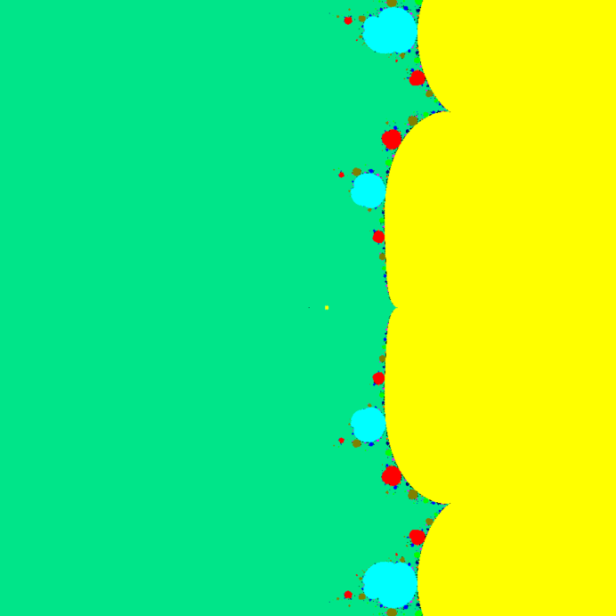
Figure 1. The $\lambda$ plane divided into the shift locus and shell components. The shift locus is shown in green. In the yellow shell component, $\lambda$ is attracted to a fixed point; in the cyan components it is attracted to a period two cycle; in the red components, a period three cycle and in the khaki components a period four cycle.

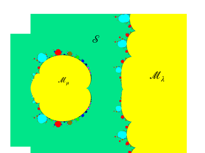
Figure 2. The $\lambda$-plane with a blow-up of the ${\mathcal{M}}_{\mu}$ region. The color coding is the same as in figure 1.

Recall that a function $f_{\lambda}$ is hyperbolic if the orbits of the asymptotic values remain bounded away from its Julia set. The interior of ${\mathcal{M}}_{\lambda}$ contains all the hyperbolic components $\Omega_{p}$ in which the orbit of $\lambda$ tends to an attracting periodic cycle of period $p$. These are called Shell components because of their shape. In [FK] it is proved that each $\Omega_{p}$ is a universal covering of the punctured disk ${\mathbb{D}}^{*}$ where the covering map is defined by the multiplier of the cycle. This map extends continuously to the boundary and there is a standard bifurcation at each rational boundary point where the multiplier is of the form $e^{2p\pi i/q}$. There is a unique point $\lambda^{*}\in\partial\Omega_{p}$ such that as $\lambda\rightarrow\lambda^{*}$ along a path in $\Omega_{p}$, the multiplier of the cycle tends to zero. This boundary point is called the virtual center since it plays the role for $\Omega_{p}$ played by the center of a hyperbolic component of the Mandelbrot set for $z^{2}+c$.

For $p\neq 1$, $\lambda^{*}$ is finite and has the additional property that $f_{\lambda^{*}}^{p-1}(\lambda^{*})=\infty$; that is, $\lambda^{*}$ is a prepole. Since the limit along a path approaching infinity from inside the asymptotic tract of an asymptotic value is the asymptotic value, $\lambda^{*}$, its iterates, where the $p^{th}$ iterate is defined by this limit, form a virtual cycle. A parameter with this property is called a virtual cycle parameter and in [FK] it is proved that every virtual center parameter on the boundary of a shell component is a virtual cycle parameter.

Remark 1.

We note that all the rational boundary points and the virtual center of a shell component $\Omega_{p}$ are accessible boundary points in the sense that the accumulation set of any path inside $\Omega_{p}$ tending to the point consists of a single point.

There is a unique component $\Omega_{1}$ in which $\lambda$ is attracted to a fixed point $q_{\lambda}(\neq 0)$. It is unbounded and, by abuse of language, we say its virtual center is infinity.

3. The Model Map

We fix $\rho=\rho_{0},|\rho_{0}|<1$, once and for all for this paper and write $f_{\lambda}$ for $f_{\lambda,\rho_{0}}$. The figures in the paper were made by taking $\rho_{0}=2/3$.

Let $\lambda_{0}$ be a point in $\Omega_{1}\subset{\mathcal{M}}_{\lambda}$ such that at the fixed point $q_{0}=q(\lambda_{0})$ of $f_{\lambda_{0}}$, $f_{\lambda_{0}}^{\prime}(q_{0})=\rho_{0}$. We remark that $\lambda_{0}$ is not uniquely defined because there is a discrete set of preimages of $\rho_{0}$ under the multiplier map. Choose one and set $Q(z)=f_{\lambda_{0}}(z)$; it is our Model map. Let $K_{0}$ be the immediate attracting basin of $q_{0}$ for $Q$.

Since the orbits of the asymptotic values either tend to $q_{0}$ or $0$, the map $Q$ is hyperbolic. Its Julia set $J_{0}$ is the common boundary of the attracting basins of $0$ and $q_{0}$; it is well known to be equal to the closure of both the set of repelling periodic points of $Q$ and the set of prepoles of $Q$. It will be convenient to identify both these sets with a space of sequences. To that end we define

Definition 2.

Let ${\mathbf{j}}_{n}=j_{1}j_{2}\ldots j_{i}\ldots j_{n}$, $j_{i}\in{\mathbb{Z}}$ be a sequence of length $n$ whose entries are integers and set ${\mathbf{J}}_{n}=\{{\mathbf{j}}_{n}\}$; let ${\mathbf{j}_{\infty}}=j_{1}j_{2}\ldots j_{i}\ldots j_{n}\ldots$, $j_{i}\in{\mathbb{Z}}$ be a sequence of infinite length whose entries are integers and set ${\mathbf{J}_{\infty}}=\{{\mathbf{j}_{\infty}}\}$. Let ${\mathbf{j}}$ denote an element of either ${\mathbf{J}}_{n}$ or ${\mathbf{J}_{\infty}}$. Define the sequence space

$$\Sigma=\{{\mathbf{j}}\in\bigcup_{n}{\mathbf{J}}_{n}\cup{\mathbf{J}_{\infty}}\cup\{\infty\}\}$$

and give it the standard sequence topology. The shift map $\sigma$ defined by dropping $j_{1}$ defines a continuous self-map on $\Sigma$.

We will use $\Sigma$ to label the inverse branches of $Q$. (See Figure 4.)

Let $l$ be a curve that joins $\lambda_{0}$ to $\infty$ in $K_{0}$; it is an asymptotic curve for $\lambda_{0}$. Set $l_{*}=\bigcup_{n\geq 1}Q^{n}(l)$; this union is a continuous curve with endpoints $q_{0}$ and $\lambda_{0}$. Although it does not matter in this section, we will see in the next section that we can choose $l$ so that it depends holomorphically on $\rho_{0}$.

Since $\mu_{0}\not\in\overline{K}_{0}$ we can define the inverse branches $R_{j}$ of $Q$, $j\in{\mathbb{Z}}$, on $K^{*}=\overline{K}_{0}\setminus l$. Note that $Q$ is periodic with period $\pi i$ and so if $q_{j}=q_{0}+j\pi i$, then $Q(q_{j})=q_{0}$; it will be convenient to choose $l$ so that each $R_{j}$ is defined in a full neighborhood of $q_{0}$ and is labeled so that $R_{j}(q_{0})=q_{j}$. Our figures are computed with $\rho_{0}=2/3$ so that $\lambda_{0}$ is real and $l$ is contained in the real axis.

We can do this by setting

$$R_{j}(w)=\frac{1}{2}\mathrm{Log}\big{(}\frac{w/\mu_{0}-1}{w/\lambda_{0}-1}\big{)}+\pi ij$$

where $\mathrm{Log}$ stands for the principal branch of the logarithm.

Since $Q$ is periodic, we can speak of adjacent poles in $J_{0}$. Let $l^{+}$ and $l^{-}$ mark the upper and lower edges of the curve $l$. Then $R_{j}$ maps $K_{0}\setminus l$ to a strip of width $\pi$ in $K_{0}$ bounded by the curves $R_{j}(l^{-})$ and $R_{j}(l^{+})$, each of which joins a pole in $J_{0}$ to infinity; moreover, the poles are adjacent. We label these poles $p_{j}$ and $p_{j+1}$ respectively. Specifically, for $w\in K^{*}$, we set

$$p_{j}=\lim_{w\to\infty\mbox{ asymptotic to }l^{-}}R_{j}(w)=\frac{1}{2}\mathrm{Log}\frac{\lambda_{0}}{\mu_{0}}+\pi ij$$

and

$$p_{j+1}=\lim_{w\to\infty\mbox{ asymptotic to }l^{+}}R_{j}(w)=\frac{1}{2}\mathrm{Log}\frac{\lambda_{0}}{\mu_{0}}+\pi i(j+1)$$

Note that although each pole is defined by two limits, the index of the pole is well defined. (See Figure 4.)

Taking one sided limits we define the images of $l$ under $R_{j}$ to be the lines

$$l_{j}=\{R_{j}(w)\quad|\ w\in l^{-}\}.$$

1. Set

   $$R_{{\mathbf{j}}_{n}}=R_{j_{1}j_{2}\ldots j_{n}}=R_{j_{1}}\circ R_{j_{2}}\circ\ldots\circ R_{j_{n}}.$$

2. We can enumerate the preimages of the fixed points in the same fashion. We set

   $$q_{{\mathbf{j}}_{n}}=q_{j_{1}j_{2}\ldots j_{n}}=R_{{\mathbf{j}}_{n}}(q_{0}).$$

3. We can enumerate the prepoles. Set

   $$p_{{\mathbf{j}}_{n}}=p_{j_{1}j_{2}\ldots j_{n}}=R_{{\mathbf{j}}_{n}}(\infty).$$

   This scheme enumerates all the prepoles by assigning each a unique element of $\Sigma$. Note that

   $$Q(p_{j_{1}j_{2}\ldots j_{n}})=p_{j_{2}\ldots j_{n}}$$

   so that $Q$ acts as a shift map $\sigma$ on the sequence.

4. We can also enumerate the repelling periodic points in $J_{0}$. If $z\in J_{0}$ and $Q^{n}(z)=z$, we can find branches $R_{j_{k}}$ such that

   $$z=R_{j_{1}j_{2}\ldots j_{n}}(z)=R_{j_{1}j_{2}\ldots j_{n}}R_{j_{1}j_{2}\ldots j_{n}}(z)=\ldots R_{j_{1}j_{2}\ldots j_{n}}(z).$$

   Or

   $$z=R_{{\mathbf{j}}_{n}}(z)=R_{{\mathbf{j}}_{n}}R_{{\mathbf{j}}_{n}}(z)=\ldots R_{{\mathbf{j}}_{n}}R_{{\mathbf{j}}_{n}}(z).$$

   That is, we can associate the infinite repeating sequence ${\mathbf{j}_{\infty}}={\mathbf{j}}_{n}{\mathbf{j}}_{n}\ldots{\mathbf{j}}_{n}\ldots$ to the point and set

   $$z=z_{\mathbf{j}_{\infty}}=R_{{\mathbf{j}}_{n}}(z_{{\mathbf{j}_{\infty}}})=Q^{n}(z_{{\mathbf{j}_{\infty}}}).$$

   Again $Q$ acts as a shift map and $Q^{n}$ leaves the infinite sequence invariant.

Proposition 1.

There is a homeomorphism from $\Sigma$ to $J_{0}$ such that for ${\mathbf{j}}\in\Sigma$ and $z\in J_{0}$, $Q(z_{{\mathbf{j}}})=z_{\sigma({\mathbf{j}})}$.

In [CJK2], using results in [FK], we proved that the finite sequence defining the prepole that is the virtual cycle parameter of a component $\Omega_{p}$ of ${\mathcal{M}}_{\lambda}$ uniquely characterizes that component. Thus, the finite sequences in $\Sigma$ are in one to one correspondence with these boundary points of ${\mathcal{M}}_{\lambda}$.

3.1. A structure for $K_{0}$

There is a linearizing homeomorphism $\phi_{0}$, defined in a largest neighborhood $\Delta=O_{\lambda_{0}}$ of $q_{0}$ to a disk ${\mathbb{D}}_{0}$ centered at the origin of radius $r_{0}$, such that $\phi_{0}(q_{0})=0$, $\phi_{0}^{\prime}(q_{0})=1$. Moreover, for $z\in\Delta$, $\phi_{0}(Q(z))=\rho_{0}\phi_{0}(z)$, $\lambda_{0}\in\partial\Delta$, $\phi_{0}$ extends continuously to the boundary and $r_{0}=|\phi_{0}(\lambda_{0})|$. The function $\log|\phi_{0}|$ is like a Green’s function for $\Delta$. The preimages of the circles $|\zeta|=r$ in ${\mathbb{D}}_{0}$ are the level curves and the preimages of the radii are the gradient curves in $\Delta$. Thus the level of $\partial\Delta$ is $r_{0}$.

The map $\phi_{0}$ depends holomorphically on $\rho_{0}$. Therefore a canonical choice for the curve $l$ used to define the branches $R_{j}$ above can be made by using the polar coordinates of ${\mathbb{D}}_{0}$. For example, if $\rho$ is real, we define $l_{*}=\phi_{0}^{-1}(t)$, $t\in[0,r_{0})\in{\mathbb{D}}_{0}$ and let $l=R_{0}(l_{*})\setminus l_{*}$. If it is not, we adjust appropriately.

Since $\mu_{0}\not\in K_{0}$, the map $\phi_{0}$ can be extended by analytic continuation to all of $K_{0}$. The curves $R_{0}^{-1}(\partial\Delta)$ have level $r_{0}/\rho_{0}$ and end at infinity. We use the level and gradient curves to define a coordinate structure on $K_{0}$ as follows. The coordinates are locally defined on preimages of $A_{0}=R_{0}(\Delta)\setminus(\Delta\cup l)$ and $\mathbf{B_{0}}=R_{0}(\overline{\Delta}\setminus\{\lambda_{0}\})$.

3.1.1. Fundamental domains

Definition 3.

We say that a region $D\subset K_{0}$, with interior $D_{0}$, is a fundamental domain for the action of $Q$ if

• for any pair $(z_{1},z_{2})\in D_{0},\,z_{1}\neq z_{2},\,,Q(z_{1})\neq Q(z_{2})$ and if

• for some integer $n\in{\mathbb{Z}}$, $\cup_{k\geq n}^{\infty}\overline{Q^{k}(D_{0})}=\overline{\Delta}$.

We now inductively define a set of fundamental domains that defines a partition of $K_{0}$ into fundamental domains. Each fundamental domain $D_{0}$ will have boundary curves that are identified by $Q$. In the process we give an enumeration scheme for these domains. The curves referred to in the description are shown in figure 3.

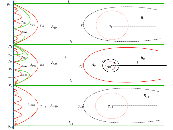
Figure 3. The model space shown with level (red) and gradient (green) curves. The dotted black curves are also level curves.

1. Let $\gamma_{0}^{*}=\gamma^{*}=\partial\Delta$. Then $Q(\Delta)\subset\Delta$ and $\Delta$ contains the positive orbit of $\lambda_{0}$. Set $\gamma_{-n}^{*}=Q^{n}(\gamma^{*})$, $n=1,\ldots,\infty$. Note that $R_{0}^{n}(\gamma_{-n}^{*})=\gamma^{*}$. These curves are nested about $q_{0}$ in $\Delta$. Any annulus $A_{-n}^{*}$ in $\Delta$ bounded by $\gamma_{-n}^{*}$ and $\gamma_{-n-1}^{*}$ is a fundamental domain for $Q$. In figure 3, $\gamma^{*}$ is drawn in black and $\gamma^{*}_{-1}$ is drawn as a dotted red curve. The annulus $A_{0}^{*}$ between them is a fundamental domain.

2. For all $j\in{\mathbb{Z}}$, set $\mathbf{B}_{j}=R_{j}(\overline{\Delta}\setminus\{\lambda_{0}\})$. In figure 3, we see that the domains $\mathbf{B}_{j}$, $j\neq 0$, are simply connected and are bounded by dotted doubly infinite black curves $\gamma_{j}=R_{j}(\gamma^{*}\setminus\{\lambda_{0}\})$; the dotted red curves inside the $\mathbf{B}_{j}$ are $R_{j}(\gamma_{-1}^{*})$; each $\mathbf{B}_{j}$ contains the preimage of the fixed point $q_{j}$. We single out the boundary curve of the domain $\mathbf{B}_{0}$, $\gamma_{0}=R_{0}(\gamma^{*}\setminus\{\lambda_{0}\})$ and color it red because, as we will see, its preimages are somewhat different from the preimages of the other $\gamma_{j}$’s. Note that $\mathbf{B}_{0}$ has a puncture at $\lambda_{0}$. The annulus $A_{0}=\mathbf{B}_{0}\setminus(\overline{\Delta}\setminus\{\lambda_{0}\})$ between $\gamma_{0}$ and $\gamma^{*}$ is a fundamental domain, and we will be particularly interested in its preimages. Note that it contains the line $l$.

3. Next, we denote the preimages of $A_{0}$ by $A_{j0}=R_{j}(A_{0})$, $j\in{\mathbb{Z}}$. To see what they look like, we look at the preimages of its boundary curves. First consider the boundary curve $\gamma^{*}$: its preimages are the curves $\gamma_{j}=R_{j}(\gamma^{*})$. The other boundary curve is $\gamma_{0}$: its preimages are the curves $\gamma_{j0}=R_{j}(\gamma_{0})$; each of these curves, drawn in red in figure 3, joins the pair of poles $(p_{j},p_{j+1})$. Now consider the preimages of the line $l$ inside $A_{0}$: these are the lines $l_{j}=R_{j}(l^{-})$ and $l_{j+1}=R_{j}(l^{+})=R_{j+1}(l^{-})$ that join the poles $p_{j}$ and $p_{j+1}$ to infinity; they are drawn in green in figure 3. Thus we see that each $A_{j0}$ is bounded by four curves, the red curves $\gamma_{j}$, $\gamma_{j0}$ and the green curves $l_{j}$ and $l_{j+1}$.

   Each $A_{j0}$ has three vertices on $\partial{K_{0}}$, the poles $p_{j}$ and $p_{j+1}$ where the lines $l_{j}$ and $l_{j+1}$ meet the ends of $\gamma_{j0}$, and infinity, the common endpoint of the doubly infinite $\gamma_{j}$ and an endpoint of each of the lines $l_{j}$ and $l_{j+1}$.

   Note that if we consider a pole as a prepole of order one, and infinity as a “prepole” of order zero, the red curves labeled by $\gamma_{i}$ join a prepole to a prepole of the same order, whereas the green curves labeled by $l_{i}$ join a prepole of order 0 to a prepole of order $1$.

   For later use we set $\mathbf{A}_{0}=\overline{\cup_{j}A_{j0}}$; it is a simply connected domain.

4. We inductively define the domains $A_{j_{1}\ldots j_{n-1}0}=R_{j_{1}}(A_{j_{2}\ldots j_{n-1}0})$. Their boundaries contain two pairs of boundary curves. The pair drawn in red, consists of $\gamma_{j_{1}\ldots j_{n-1}0}$ which joins adjacent prepoles of order $n-1$, and $\gamma_{j_{2}\ldots j_{n-1}0}$ which joins a prepole of order $n-2$ to itself if $j_{n-1}\neq 0$ and joins two adjacent prepoles of order $n-2$ if $j_{n-1}=0$. The other pair, drawn in green, consists of $l_{j_{1}\ldots j_{n-2}j_{n-1}0}$ and $l_{(j_{1}+1)j_{2}\ldots j_{n-2}j_{n-1}0}$, each joining a prepole of order $n-2$ to a prepole of order $n-1$. If $j_{n-1}=0$, all four boundary prepoles are distinct; if not, the prepoles of order $n-1$ are the same.

   The domains $A_{000}$ and $A_{100}$ are shown in figure 3. Although not all the curves are labeled, the red curves are preimages of $\gamma_{0}$ and the green curves are preimages of $l$.

   Again, for later use, we define the simply connected domains

   $$\mathbf{A}_{j_{1}\ldots j_{n-1}0}=R_{j_{1}}(\mathbf{A}_{j_{2}\ldots j_{n-1}0})$$

   for all $n>1$.

5. Unlike the preimages of $\gamma_{0}$ which join two adjacent poles, the curves $\gamma_{ji}=R_{j}(\gamma_{i})$, $i\neq 0$ are curves that join a pole to itself. This is because of the way we have defined the $R_{i}$. The pole $p_{j}$ is one endpoint of each the curves $\gamma_{(j-1)0}$ and $\gamma_{j0}$. The curves $\gamma_{ji}$, $i>0$, are loops that come in to $p_{j}$, tangent to, and under $\gamma_{j0}$ while the curves $\gamma_{(j-1)i}$, $i<0$, are loops that come in to $p_{j}$, tangent to, and under $\gamma_{(j-1)0}$. Thus, in the preimage, $R_{i}(K_{0})$, the curves $\gamma_{ji}$ are tangent to the pole $p_{i}$ for $j\geq 0$ and tangent to the pole $p_{i+1}$ for $j\leq 0$.

   Therefore the loops $\gamma_{ji}$, $j\neq 0$, bound simply connected domains $\mathbf{B}_{ji}=R_{j}(\mathbf{B}_{i})$. They are tesselated by the fundamental annuli $B_{ji}^{k}=R_{ji}(A_{-k}^{*})$, $k\geq 0$ and each $\mathbf{B}_{ji}$ contains a curve that is a preimage of the line $l_{*}$. The disjoint domains $\mathbf{B}_{ji}$ form an infinite cluster at each pole. For considerations of space and clarity, we haven’t included them in the figure.

   Note that the fundamental domains $B_{ji}^{k}$ are analogous to the fundamental domains $A_{j0}$ whereas the unions of fundamental domains $\mathbf{B}_{ji}$ are analogous to the unions of fundamental domains $\mathbf{A}_{{\mathbf{j}}_{n-1}0}$. We will preserve this analogy and notation in the inductive definition below.

6. We inductively define the domains $\mathbf{B}_{{\mathbf{j}}_{n}}=R_{j}(\mathbf{B}_{{\mathbf{j}}_{n-1}})$. Thus ${\mathbf{j}}_{n}$ has the form $j{\mathbf{j}}_{n-2}i$, $i\neq 0$. For each $j$, if $i>0$, the $\mathbf{B}_{{\mathbf{j}}_{n}}$ cluster at the prepole $p_{{\mathbf{j}}_{n-2}i}$ and if $i<0$ they cluster at the prepole $p_{{\mathbf{j}}_{n-2}(i+1)}$. Each has an outer biinfinite boundary curve, $\gamma_{{\mathbf{j}}_{n}}$, both of whose endpoints are at the same pole and an interior curve $l_{{\mathbf{j}}_{n}}$, joining the pole $p_{{\mathbf{j}}_{n-2}i}$ to $q_{{\mathbf{j}}_{n}}$. Each of the domains $\mathbf{B}_{{\mathbf{j}}_{n}}$ is a union of fundamental domains $B_{{\mathbf{j}}_{n}}^{k}$.

7. We remark that the admissibility condition for the $\mathbf{A}_{{\mathbf{j}}_{n}}$ is that the rightmost entry in the sequence ${\mathbf{j}}_{n}$ is always zero while the condition for the $\mathbf{B}_{{\mathbf{j}}_{n}}$ is that the rightmost entry is never zero. The geometry of these regions is different. The $\mathbf{A}_{{\mathbf{j}}_{n}}$ have infinitely many vertices at infinitely many distinct prepoles. Each interior fundamental domain has vertices at three or four distinct prepoles. The $\mathbf{B}_{{\mathbf{j}}_{n}}$, on the other hand, have only one vertex at a single prepole, or infinity if $n=1$, where all the boundary curves meet. The fundamental domains contained in them are annuli, the outermost of which has a prepole on its boundary.

3.1.2. The Coordinates

We extend the map $\phi_{0}$ defined above to all of $K_{0}$ by analytic continuation. Continuing across the boundary of $\Delta$ we have

$$\phi_{0}^{-1}(\{\zeta\,|\,r_{0}\leq|\zeta|\leq r_{0}/\rho\})=\overline{A_{0}}.$$

We use the closure here to include the boundary curves. We extend the map to all of $K_{0}\setminus\{\lambda_{0}\}$ in the obvious way: if $z$ is in a fundamental domain $Q^{-n}(A_{0})$ for any $n$ inverse branches, we set $\rho^{n}\phi_{0}(z)=\phi_{0}(Q^{n}(z))$.

We define coordinates for $K_{0}$ in terms of local coordinates in the fundamental domains described above.

1. The curves $\phi_{0}^{-1}(|\zeta|=r)$ are the level curves of level $r$ in $K_{0}$. The level of $\gamma^{*}$ is $r_{0}$ and the level of $\gamma_{j}$ is $r_{0}/\rho$.

   The outer boundary of each $\mathbf{B}_{{\mathbf{j}}_{n}}$ has level $r_{0}/\rho^{n}$; passing through the interior fundamental domains, the levels decrease to zero by powers of $\rho^{k}$. In each $\mathbf{A}_{{\mathbf{j}}_{n}}$ the levels go from $r_{0}/\rho^{n-1}$ to $r_{0}/\rho^{n}$ and the same is true in the interior fundamental domains.

2. The gradient curves are preimages of the radii $\theta=\theta_{0}$ for a fixed $\theta_{0}\in{\mathbb{R}}$ under the map $\phi_{0}^{-1}(re^{i\theta})$. For example, each of the fundamental domains $A_{{\mathbf{j}}_{n}}$ has four boundary curves; one pair of opposite curves, labeled with $\gamma$’s and shown in red in figure 3, are level curves and the other pair of opposite curves, labeled with $l$’s and shown in green in figure 3, are gradient curves along which the level rises from $r_{0}/\rho^{n-1}$ to level $r_{0}/\rho^{n}$.

3. The level and gradient curves define a set of local coordinates in $K_{0}$: the preimages of the circles and radii in ${\mathbb{D}}_{0}$ under the extension of $\phi_{0}$ pull back to each fundamental domain. We denote the coordinates of the point $z\in K_{0}$ by

   $$z=(X_{{\mathbf{j}}_{n}},r,\theta+\pi(n-1))$$

   where $X_{{\mathbf{j}}_{n}}=\overline{A_{{\mathbf{j}}_{n}}}$ if ${\mathbf{j}}_{n}=j_{1}\ldots j_{n-1}0$ and $X_{{\mathbf{j}}_{n}}=\overline{B_{{\mathbf{j}}_{n}}^{k}}$ if ${\mathbf{j}}_{n}=j_{1}\ldots j_{n-1}j$, $j\neq 0$. Because $k$ can be read off from $r\in[0,\infty)$, it is enough to write $X_{{\mathbf{j}}_{n}}$. We let $\theta\in[-\pi,\pi)$ and note that because the inverse branches are defined as one sided limits on the boundaries of the fundamental domains, the $\theta$ coordinate varies continuously across common boundaries.

Theorem 2.

Every point $z\in K_{0}$, $z\neq\lambda_{0}$, is in either a unique $A_{{\mathbf{j}}_{n}}$ or a unique $B_{{\mathbf{j}}_{n}}^{k}$ or on the boundary of two such domains: either the common boundary of some $A_{{\mathbf{j}}_{n}}$ and some $A_{{\mathbf{j}}_{n+1}}$ where ${\mathbf{j}}_{n+1}={\mathbf{j}}_{n}0$, or the common boundary of an $A_{{\mathbf{j}}_{n}}$ and a $B_{{\mathbf{j}}_{n-1}}^{0}$ where ${\mathbf{j}}_{n}={\mathbf{j}}_{n-1}j_{n}$, $j_{n}\neq 0$ or the common boundary of a $B_{{\mathbf{j}}_{n-1}}^{k}$ and a $B_{{\mathbf{j}}_{n-1}}^{k+1}$.

Proof.

Let $z\in K_{0}$, $z\neq\lambda_{0}$. Since every such $z$ is attracted to $q_{0}$ and has infinitely many preimages, there is an $m$ such that $Q^{m}(z)\in\Delta\cup(\partial\Delta\setminus\{\lambda_{0}\})$. If $\zeta=Q^{m}(z)\in\Delta$, there is a unique set of preimages $R_{j}$ such that $z=R_{{\mathbf{j}}_{m}}(\zeta)$. If $\zeta\in(\partial\Delta\setminus\{\lambda_{0}\})$ the $\theta$ coordinate is defined as a one sided limit for each preimage, and the limits agree on the boundary curves. ∎

3.1.3. The Tree in $K_{0}$

In this section we use the domains $\mathbf{A}_{{\mathbf{j}}_{n}}$ which are unions of the fundamental domains $A_{{\mathbf{j}}_{n}0}$ to define a tree in $K_{0}$. For readability, we will say a level curve of level $r_{0}/\rho^{n}$ has level $n$.

Among the boundary curves of the union $\mathbf{A}_{{\mathbf{j}}_{n}}$, there is a distinguished boundary curve of level $n$; it is a preimage of $\gamma_{0}$ under the map $R_{{\mathbf{j}}_{n}}$. The remaining infinitely many boundary curves of the union have level ${n+1}$ and are images under the maps $R_{{\mathbf{j}}_{n}j}$. Note that the non-distinguished boundary curves of $\mathbf{A}_{{\mathbf{j}}_{n}}$ of level $n$ are also boundaries of some $\mathbf{B}_{{\mathbf{j}}_{n}}$. At level $n=1$ we will fix a root node on $\gamma_{0}$. On each $\gamma_{{\mathbf{j}}_{n}0}$ of level $n$, $n>1$, we will define the preimage of the root to be a node of the tree. We call these interior nodes. We will also put nodes at every prepole of every order on the tree.

The children of the interior node of level $n$ are the interior nodes of level $n+1$, a prepole of level $n$ and infinitely many prepoles of level $n+1$. We will define branches of the tree that connect a node to each of its children. The nodes that are prepoles have no children and are called leaves of the tree. Each interior node has only one parent and each prepole node has two parents. Paths through the tree start at the root and consist of a connected set of branches joining nodes in the tree. Some will be finite, ending at leaves and others will be infinite.

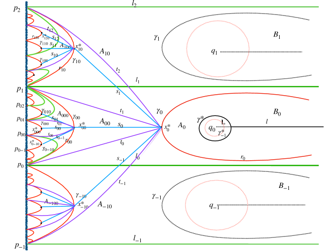
Figure 4. The fundamental domains of the model space with the tree.

For the explicit construction of the tree, (see figure 4), fix a point $x_{0}^{*}$ on the boundary curve $\gamma_{0}$ of the domain $A_{0}$. It has level $1$ and is the first node, or root of the tree. For each $n>1$, and each ${\mathbf{j}}_{n}={\mathbf{j}}_{n-1}0$, the interior nodes of level $n$ are defined as the points $x_{{\mathbf{j}}_{n-1}0}^{*}=R_{{\mathbf{j}}_{n}}(x_{0}^{*})$. The prepoles of all orders are leaves of the tree.

The first step of the construction is to define a tree $T^{*}$. Join the root $x_{0}^{*}$ to each of the nodes $x_{j0}^{*}$, $j\in{\mathbb{Z}}$, by a branch $s_{j}$ and join it to the pole $p_{j}$ by a branch $t_{j}$. Also define the segment $r_{0}$ of $\gamma_{0}$ from $x_{0}^{*}$ to infinity, asymptotic to the line $l_{0}$ as a branch joining the root to the “prepole” infinity. The root with these branches connected to the leaves is a small tree $T^{*}$ contained in $\mathbf{A}_{0}$. Since the domain $\mathbf{A}_{0}$ admits a hyperbolic metric, we may choose $s_{j}$ as geodesics in the hyperbolic metric and take the $t_{j}$ and $r_{0}$ along the level curves. The hyperbolic lengths of the $s_{j}$ go to infinity with $|j|$ while the lengths of the $t_{j}$ and $r_{0}$ are always infinite.

Now define a small tree at each node $x_{{\mathbf{j}}_{n}0}^{*}$, and contained in $\mathbf{A}_{{\mathbf{j}}_{n}0}$, by $T_{{\mathbf{j}}_{n}}^{*}=R_{{\mathbf{j}}_{n}}(T^{*})$. Note that as often happens, the spatial relationship of the nodes in the tree is dual to the dynamic relationship. The nodes $x^{*}_{j_{1}k0}$, $k\in{\mathbb{Z}}$, are children of the node $x^{*}_{{j_{1}}0}$, whereas the nodes $x^{*}_{{kj_{1}}0}$ which are preimage of $x_{j_{1}0}$ are not. Thus the children of the parent node $x_{{\mathbf{j}}_{n}0}^{*}$ are the nodes $x_{{\mathbf{j}}_{n}k0}^{*}$ and not the nodes $x_{k{\mathbf{j}}_{n}0}^{*}$. The tree has branches $s_{{\mathbf{j}}_{n}}$ joining the parent node $x_{{\mathbf{j}}_{n}0}^{*}$ to its interior children $x^{*}_{j_{1}k0}$, a branch $r_{{\mathbf{j}}_{n}0}$ joining it to the prepole $p_{{\mathbf{j}}_{n}}$ and branches $t_{{\mathbf{j}}_{n}k}$ joining it to the prepoles $p_{{\mathbf{j}}_{n}k}$. Because the $R_{j}$ are biholomorphic, the hyperbolic lengths of the branches are preserved.

Finally, joining all these small trees together, we obtain the full tree

$$T_{\infty}^{*}=\bigcup_{n}\cup_{{\mathbf{j}}_{n}}(T_{{\mathbf{j}}_{n}}).$$

If ${{\mathbf{j}_{\infty}}}$ is periodic with period $n$, there is a sequence ${\mathbf{j}}_{n}=j_{1}\ldots j_{n}$ such that ${{\mathbf{j}_{\infty}}}={\mathbf{j}}_{n}{\mathbf{j}}_{n}{\mathbf{j}}_{n}\ldots$. By the periodicity, $j_{1+n}=j_{1}$, so that the node $x^{*}_{j_{1}{\mathbf{j}}_{n}0}$ is a direct descendant of the node $x^{*}_{j_{1}0}$. This means that there is a path $\tau_{{\mathbf{j}}_{n}}=s_{j_{1}}\cup s_{j_{1}j_{2}}\cup\ldots s_{j_{1}\ldots j_{n-1}}$ from the root to the node. It has finite hyperbolic length. Note, however, as we remarked above, applying $R_{j_{i}}$ to successively obtain the nodes $x^{*}_{j_{n}0},x^{*}_{j_{n-1}j_{n}0},\ldots,x^{*}_{j_{2}\ldots j_{n-1}j_{n}0}$, yields a collection of nodes that are not direct descendants of $x^{*}_{j_{1}0}$.

The path

$$\tau_{{\mathbf{j}}_{n}{\mathbf{j}}_{n}}=R_{{\mathbf{j}}_{n}}(\tau_{{\mathbf{j}}_{n}})=R_{{\mathbf{j}}_{n}}(s_{j_{1}})\cup R_{{\mathbf{j}}_{n}}(s_{j_{1}j_{2}})\cup\ldots R_{{\mathbf{j}}_{n}}(s_{j_{1}\ldots j_{n-1}})$$

joins $x^{*}_{{\mathbf{j}}_{n}0}$ to $x^{*}_{{\mathbf{j}}_{n}{\mathbf{j}}_{n}0}$ and has the same hyperbolic length as $\tau_{{\mathbf{j}}_{n}}$. Iterating, we obtain a path $\tau_{{\mathbf{j}_{\infty}}}$ of infinite length that is invariant under $R_{{\mathbf{j}}_{n}}$.

All but the first segment of this path are separated from the root by the level curve $\gamma_{j_{1}0}$ so any accumulation point of the path lies in the Julia set between the poles $p_{j_{1}}$ and $p_{j_{1}+1}$. Thus the path remains inside a compact domain bounded by $\gamma_{j_{1}0}$ and the Julia set boundary of $K_{0}$. This implies that the Euclidean lengths of subpaths making up $\tau_{{\mathbf{j}}}$ tend to zero, and since $Q$ is hyperbolic, that the full path has a unique endpoint.

Thus if ${\mathbf{j}_{\infty}}$ is periodic of period $n$, the path in the tree with unique endpoint $z_{{\mathbf{j}_{\infty}}}$ is invariant under $Q^{n}$ and corresponds to a repelling periodic point of $Q$ in $J_{0}$ whose combinatorics agree with those defined in Proposition 1.

If ${\mathbf{j}_{\infty}}$ is preperiodic, ${\mathbf{j}}={\mathbf{j}}_{m}{\mathbf{j}}_{n}{\mathbf{j}}_{n}{\mathbf{j}}_{n}\ldots$, we can construct a periodic infinite subpath of $\tau_{{\mathbf{j}_{\infty}}}$ beginning at $x_{{\mathbf{j}}_{m}}^{*}=R_{{\mathbf{j}}_{m}}(x_{0}^{*})$, instead of the root, so that it is invariant under $R_{{\mathbf{j}}_{n}}$. The argument above shows it also has a unique preperiodic endpoint.

4. The Shift Locus

In the shift locus ${\mathcal{S}}$, both asymptotic values are attracted to the origin. If $\lambda\in{\mathcal{S}}$, we can define a linearizing map $\phi_{\lambda}$ from the attractive basin $A_{\lambda}$ of the origin to the disk ${\mathbb{D}}_{0}$ that is injective on a neighborhood $O_{\lambda}$ of the origin. Neither $\lambda$ nor $\mu$ lies in $O_{\lambda}$ and one or both lie on $\partial O_{\lambda}$.

We divide ${\mathcal{S}}$ into disjoint subsets as follows

$${\mathcal{S}}_{\lambda}^{0}=\{\lambda\in{\mathcal{S}}\,|\,\,\mu\in\partial O_{\lambda},\,\lambda\not\in\partial O_{\lambda}\},$$

$${\mathcal{S}}_{\mu}^{0}=\{\lambda\in{\mathcal{S}}\,|\,\,\lambda\in\partial O_{\lambda},\,\mu\not\in\partial O_{\lambda}\},\mbox{ and }$$

$${\mathcal{S}}_{*}=\{\lambda\in{\mathcal{S}}\,|\,\,\lambda\in\partial O_{\lambda},\,\mu\in\partial O_{\lambda}\},$$

We normalize the map so that if $z_{0}$ equal to the asymptotic value on the boundary and $z\in O_{\lambda}$ then

$$\phi_{\lambda}(0)=0,\phi_{\lambda}(z_{0})=\phi_{0}(\lambda_{0})=r_{0},\mbox{ and }\phi_{\lambda}(f_{\lambda}(z))=\rho\phi_{\lambda}(z).$$

Note that this normalization agrees with our normalization of $\phi_{0}$, the linearizing map for the model $Q$; that is, both map the asymptotic value to the point $r_{0}$ on the real axis.

We restrict our discussion here to ${\mathcal{S}}_{\lambda}^{0}$ but there is a comparable discussion for ${\mathcal{S}}_{\mu}^{0}$.

4.1. Coordinates in the dynamic plane $A_{\lambda}$

The scheme we defined above for tesselating the attracting basin $K_{0}$ of $Q=f_{\lambda_{0}}$ works equally well in a subdomain of the attractive basin of zero, $A_{\lambda}$, for $\lambda\in{\mathcal{S}}_{\lambda}^{0}$.

Theorem 3.

Given $\lambda\in{\mathcal{S}}_{\lambda}^{0}$, there is a coordinate structure defined on a subdomain $\widehat{A}_{\lambda}$ of $A_{\lambda}$. More precisely, there is an integer $N$ such that the basin of the origin of $f_{\lambda}$, $A_{\lambda}$, contains a subdomain $\widehat{A}_{\lambda}$ tesselated by fundamental domains $\alpha_{\lambda,{\mathbf{j}}_{n-1}0}$ and $\beta_{\lambda,{\mathbf{j}}_{n-1}i}^{k}$, $i\neq 0$, $k\geq 0$ and $n\leq N$. The boundary curves of these regions are level and gradient curves defined by using a normalized linearizing function $\phi_{\lambda}$ near the origin, and pulling back a radius and circle containing $\phi_{\lambda}(\mu)$ to $A_{\lambda}$. The geometric properties of the $\alpha_{\lambda,{\mathbf{j}}_{n-1}0}$ and $\beta_{\lambda,{\mathbf{j}}_{n-1}i}^{k}$ are analogous to those of the fundamental domains $A_{{\mathbf{j}}_{n-1}0,\lambda}$ and $B_{{\mathbf{j}}_{n-1}i,\lambda}^{k}$ domains in $K_{0}$. The coordinates in $\widehat{A}_{\lambda}$ are $(\sigma_{{\mathbf{j}}_{n}},r,\theta+\pi(n-1))$ where $r\in[0,\infty),\theta\in[-\pi,\pi)$ and $\sigma_{{\mathbf{j}}_{n}}=\sigma_{{\mathbf{j}}_{n-1}i}$ stands for $\alpha_{\lambda,{\mathbf{j}}_{n-1}0}$ if $i=0$ and $\beta_{\lambda,{\mathbf{j}}_{n-1}i}^{k}$ for some $k$ depending on $r$ for $i\neq 0$.

Proof.

For $\lambda\in{\mathcal{S}}_{\lambda}^{0}$, the attractive basin of zero, $A_{\lambda}$ contains both asymptotic values. By definition, the linearizing map $\phi_{\lambda}$ is a homeomorphism from $O_{\lambda}$, an open neighborhood of the origin with $\mu$ on its boundary, onto the disk ${\mathbb{D}}_{0}$ of radius $r_{0}$. It is normalized so that $\phi_{\lambda}(0)=0$ and $\phi_{\lambda}(\mu)=\phi_{0}(\lambda_{0})=r_{0}$. Extending $\phi_{\lambda}$ by analytic continuation, the analogues of the domains $A_{{\mathbf{j}}_{n}}$ and $B_{{\mathbf{j}}_{n}}^{k}$ can be defined as in section 3.1.2 until, for some $n=N$, one of them contains $\lambda$. That is, $r_{0}/\rho^{N-1}<|\phi_{\lambda}(\lambda)|\leq r_{0}/\rho^{N}$. The level and gradient curves are well defined in these domains by the branches of $\phi_{\lambda}^{-1}$.

To this end, we use the map $\xi_{\lambda}=\phi_{0}^{-1}\circ\phi_{\lambda}:O_{\lambda}\rightarrow O_{\lambda_{0}}$ that we defined In [CJK2]. The inverse map, $\xi_{\lambda}^{-1}$, extends, as a homeomorphism from a subset, $K_{0}(\lambda)$ to a largest subset $\widehat{A}_{\lambda}$ of $A_{\lambda}$ that contains $\lambda$. Therefore $\xi_{\lambda}^{-1}$ is defined on the fundamental domains $A_{{\mathbf{j}}_{n}}$ and $B_{{\mathbf{j}}_{n}}^{k}$ tesselating $K_{0}$, $k\geq 0$, $n\leq N$, where $N$ is the largest integer such that $|\phi_{\lambda}(\lambda)|\leq r_{0}/\rho^{N}$.

Set $\alpha_{\lambda,{\mathbf{j}}_{n}}=\xi_{\lambda}^{-1}(A_{{\mathbf{j}}_{n}})$ and $\beta_{\lambda,{\mathbf{j}}_{n}}^{k}=\xi_{\lambda}^{-1}(B_{{\mathbf{j}}_{n}}^{k})$. The boundary curves of these domains are, by definition, level and gradient curves for $A_{\lambda}$ and the relative levels correspond, via the map $\xi_{\lambda}^{-1}$, to the levels of the corresponding curves in $K_{0}$. Moreover, since we can define inverse branches $R_{\lambda,j}$ of $f_{\lambda}$ on $\widehat{A}_{\lambda}$ using the relation $R_{\lambda,j}=\xi_{\lambda}\circ R_{j}\circ\xi_{\lambda}^{-1}$, the indexing is consistent with the model. Thus we obtain a coordinate $(\sigma_{{\mathbf{j}}_{n}},r,\theta+\pi(n-1))$ for $\widehat{A}_{\lambda}$. ∎

We can also use the map $\xi_{\lambda}^{-1}$ to obtain a tree in $\widehat{A}_{\lambda}$, $T^{*}_{\lambda}=\xi_{\lambda}^{-1}(T^{*}_{\infty}\cap K_{0}^{\lambda})$. The root of this tree is $x_{\lambda}^{*}=\xi_{\lambda}^{-1}(x_{0}^{*})$. Its nodes are defined similarly. Note that some of images of infinite paths in $T_{\infty}$ are truncated and so are finite in $T^{*}_{\lambda}$.

4.2. Coordinates in ${\mathcal{S}}_{\lambda}^{0}$

In [CJK2] we proved

Theorem 4.

There is a homeomorphism $E:{\mathcal{S}}_{\lambda}^{0}\rightarrow K_{0}\setminus\overline{\Delta}$. Thus ${\mathcal{S}}_{\lambda}^{0}$ is homeomorphic to an annulus ${\mathbb{A}}$. If $I$ is the inner boundary of ${\mathbb{A}}$, $I=\partial\Delta$ and $E^{-1}$ extends continuously to all points on $I$ except $\lambda_{0}$. The point $E^{-1}(\lambda_{0})$ corresponds to the parameter singularity $\lambda=0$ on the inner boundary of ${\mathcal{S}}_{\lambda}^{0}$ where the function $f_{\lambda}$ is not defined. The outer boundary of $E^{-1}({\mathbb{A}})$ is contained in $\partial{\mathcal{M}}_{\lambda}$ and contains all the virtual centers.

To define the map $E$ we use the maps $\phi_{0}$, $\phi_{\lambda}$ and $\xi_{\lambda}=\phi_{0}^{-1}\circ\phi_{\lambda}$, and set $E(\lambda)=\xi_{\lambda}(\lambda)$. It is not difficult to prove the map is injective. We then prove the map is a homeomorphism by the following construction: to each $\zeta\in K_{0}\setminus\Delta$, $\zeta\neq\lambda_{0}$, we inductively construct a sequence of covering spaces of $K_{0}\setminus\{\lambda_{0},\zeta\}$ and corresponding covering maps. Using quasiconformal surgery, we prove the direct limit of this process is a map in ${\mathcal{S}}_{\lambda}^{0}$.

The inverse holomorphic homeomorphism $E^{-1}$ can be used to define a tesselation and coordinates in ${\mathcal{S}}_{\lambda}^{0}$. For each sequence $\mathbf{j_{n}}$, define ${\mathcal{A}}_{\mathbf{j}_{n}}=E^{-1}(A_{{\mathbf{j}}_{{n-1}0}})$ and ${\mathcal{B}}_{\mathbf{j}_{n}}^{k}=E^{-1}(B_{{\mathbf{j}}_{n-1}i}^{k})$, $i\neq 0$, $k\geq 0$. This identification immediately gives us, (see Figure 5),

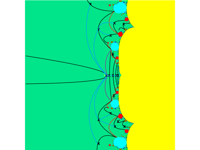
Figure 5. The parameter space with some of the level curves in black, gradient curves in red and paths from the tree in purple.

Theorem 5.

Each point $\lambda\in{\mathcal{S}}_{\lambda}^{0}$ has a unique coordinate $\lambda=(\mathcal{X}_{\mathbf{j}_{n}},r,\theta)$ where $\mathcal{X}_{\mathbf{j}_{n}}$ is either ${\mathcal{A}}_{\mathbf{j}_{n}}$ or ${\mathcal{B}}_{\mathbf{j}_{n}}^{k}$, $r\in[0,\infty),\theta=t+(n-1)\pi\in{\mathbb{R}}$, $0\leq t<\pi$.

5. The boundaries of $K_{0}$ and ${\mathcal{M}}_{\lambda}$

We are now ready to prove our main result.

Theorem 6.

The injective holomorphic map $E:{\mathcal{S}}_{\lambda}^{0}\rightarrow K_{0}\setminus\overline{\Delta}$ extends continuously to the virtual centers of $\partial{\mathcal{S}}_{\lambda}^{0}$ and maps them to prepoles of $Q$ with the same itinerary.

Proof.

Fix a finite sequence ${\mathbf{j}}_{n}$ and let $\tau(t)$, $t\in[0,1]$ be a path in the tree $T_{\infty}$ that ends at the prepole $p_{{\mathbf{j}}_{n}}$. That is, it passes from the root to the node $x^{*}_{{\mathbf{j}}_{n}0}$ and its last branch $r_{{\mathbf{j}}_{n}0}$ goes from $x^{*}_{{\mathbf{j}}_{n}0}$ to the prepole $p_{{\mathbf{j}}_{n}}$ along the level curve $\gamma_{{\mathbf{j}}_{n}0}$. The map $E^{-1}$ then maps $\tau(t),t\in[0,1)$, to a path $\lambda(t)\in{\mathcal{S}}_{\lambda}^{0}$.

We claim that the accumulation set of $\lambda(t)$ as $t$ goes to $1$ is a single point and that this point is a virtual cycle parameter.

Let $\lambda_{\infty}\in\partial{\mathcal{S}}_{\lambda}^{0}$ be an accumulation point of $\lambda(t)$ as $t$ goes to $1$ and let $t_{m}$ be sequence tending to $1$ such that $\lambda_{m}=\lambda(t_{m})$ has limit $\lambda_{\infty}$. Since we are only interested in $\tau(t)$ for $t$ close to $1$, we may assume all the points $\tau_{m}=\tau(t_{m})$ belong to the last edge $t_{{\mathbf{j}}_{n}}$.

Note that the attractive basins $A_{\lambda}$ of $f_{\lambda}$ and the boundary curves defining their tesselations by fundamental domains $\alpha_{\lambda,{\mathbf{j}}_{n-1}0}$ and $\beta_{\lambda,{\mathbf{j}}_{n-1}i}^{k}$, $i\neq 0$, in $\widehat{A}_{\lambda}\subset A_{\lambda}$ all move holomorphically with $\lambda$.

In particular, the unions of these domains $\boldsymbol{\alpha}_{\lambda,{\mathbf{j}}_{n-1}0}=\xi_{\lambda}^{-1}(\mathbf{A}_{{\mathbf{j}}_{n-1}0})$ and $\boldsymbol{\beta}_{\lambda,{\mathbf{j}}_{n-1}i}=\xi_{\lambda}^{-1}(\mathbf{B}_{{\mathbf{j}}_{n-1}i})$, $i\neq 0$, and their prepole boundary points, including the prepole $p_{\lambda,{\mathbf{j}}_{n}}$, move holomorphically. Thus, as $m$ goes to infinity, the functions $f_{\lambda_{m}}$ converge to $f_{\lambda_{\infty}}$ and the prepoles $p_{\lambda_{m},{\mathbf{j}}}$ converge to a prepole $p_{\lambda_{\infty,\mathbf{j}_{n}}}$ of $f_{\lambda_{\infty}}$. Moreover, $\tau_{m}$ is on a level curve in $K_{0}$, and the images under $\xi_{\lambda}$ of the level curves in $K_{0}$ are level curves in $A_{\lambda}$, so each $\lambda_{m}=\xi_{\lambda_{m}}(\tau_{m})$ is on a level curve of the same level. The level curves in $A_{\lambda_{m}}$ containing $\lambda_{m}$ have endpoints at prepoles so that $\lim_{m\to\infty}\xi_{\lambda_{m}}(\tau_{m})=p_{\lambda_{\infty},{\mathbf{j}}_{n}}$. Therefore either $\lambda_{\infty}\in A_{\lambda_{\infty}}$ so that $\lambda_{\infty}\in{\mathcal{S}}_{\lambda}^{0}$, or

$$|\lambda_{m}-p_{\lambda_{\infty,\mathbf{j}_{n}}}|\leq|\lambda_{m}-p_{\lambda_{m},{\mathbf{j}}_{n}}|+|p_{\lambda_{m},{\mathbf{j}}_{n}}-p_{\lambda_{\infty,\mathbf{j}_{n}}}|\rightarrow 0\text{ as }m\to\infty.$$

The first possibility cannot happen since we assumed $\lambda_{\infty}\not\in{\mathcal{S}}_{\lambda}^{0}$. The second says that $\lambda_{\infty}$ is a virtual cycle parameter. Since the sequence $t_{m}$ was arbitrary and the prepoles of any given order form a discrete set, the limit is independent of the sequence and thus unique. ∎

We turn now to the periodic points in the Julia set of $Q$ and show that the map $E^{-1}$ extends to them. The proof is similar to the above.

Theorem 7.

The injective holomorphic map $E^{-1}:K_{0}\setminus\overline{\Delta}\rightarrow{\mathcal{S}}_{\lambda}^{0}$ extends continuously to the repelling periodic points in $\partial K_{0}$ and maps them to points in $\lambda\in\partial{\mathcal{S}}_{\lambda}^{0}$ for which $f_{\lambda}$ has a parabolic cycle of the same period.

Proof.

Let ${\mathbf{j}_{\infty}}={\mathbf{j}}_{n}{\mathbf{j}}_{n}\ldots$ be a periodic infinite sequence and let $z_{{\mathbf{j}_{\infty}}}\in\partial K_{0}$ be the repelling point of order $n$ in the Julia set of $Q$ corresponding to this sequence. Let $\tau_{{\mathbf{j}_{\infty}}}(t)$, $t\in[0,1)$ be the infinite path in $T_{\infty}$ corresponding to the sequence. It is invariant under $Q^{n}$ and, since $Q$ is hyperbolic, its endpoint in $J_{0}$ is well defined and is the repelling periodic point $z_{{\mathbf{j}}}$.

Let $\lambda(t)=E^{-1}(\tau_{{\mathbf{j}_{\infty}}}(t))$. We claim this path lands on $\partial{\mathcal{S}}_{\lambda}^{0}$ as $t$ goes to $1$. Let $\lambda_{\infty}$ be any point in the accumulation set of the path and let $t_{m}$ be a sequence tending to $1$ such that $\lambda_{m}=\lambda(t_{m})$ has limit $\lambda_{\infty}$.

For each $m$, there is an integer $k(m)$ such that if ${\mathbf{j}}_{k(m)}$ is a truncation of the periodic sequence ${\mathbf{j}_{\infty}}$ after $k(m)$ repetitions of ${\mathbf{j}}_{n}$, $\lambda_{m}\in{\mathcal{A}}_{{\mathbf{j}}_{k(m)}}\subset{\mathcal{S}}_{\lambda}^{0}$. This means we also have $\lambda_{m}\in\boldsymbol{\alpha}_{\lambda_{m},{\mathbf{j}}_{k(m)}}\subset\widehat{A}_{\lambda_{m}}$ and $\xi_{\lambda_{m}}(\lambda_{m})\in\mathbf{A}_{{\mathbf{j}}_{k(m)}}\subset K_{0}$. Let $\widehat{\tau}_{{\mathbf{j}}_{k(m)}}\in T_{\infty}$ be the tree $\tau_{{\mathbf{j}_{\infty}}}$ in $K_{0}$ up to the node $x_{{\mathbf{j}}_{k(m)}0}^{*}$, and having as its final branch, $r_{{\mathbf{j}}_{k(m)}}$, the level curve from the node to the prepole $p_{{\mathbf{j}}_{k(m)}}$. The last fundamental domain it passes through is $\mathbf{A}_{{\mathbf{j}}_{k(m)}}$.

Using the map $\xi_{\lambda}^{-1}$ we can pull back $\widehat{\tau}_{{\mathbf{j}}_{k(m)}}$ to a tree $\widehat{\tau}_{\lambda_{m},{\mathbf{j}}_{k(m)}}\subset\widehat{A}_{\lambda_{m}}$. The last fundamental domain it passes through is $\boldsymbol{\alpha}_{{\mathbf{j}}_{k(m)}}$ and this fundamental domain contains $\lambda_{m}$. We can modify the branch of $\widehat{\tau}_{\lambda_{m},{\mathbf{j}}_{k(m)}}$ in $\boldsymbol{\alpha}_{{\mathbf{j}}_{k(m)}}$ so that it passes through $\lambda_{m}$. We will do this, and by abuse of notation, denote the modified tree by $\widehat{\tau}_{\lambda_{m},{\mathbf{j}}_{k(m)}}$ again.

Everything is holomorphic in $\lambda$, and as $k$ goes to infinity, ${\mathbf{j}}_{k(m)}\to{\mathbf{j}_{\infty}}$, so the prepoles $p_{{\mathbf{j}}_{k(m)}}\in J_{0}$ tend to the repelling periodic point $z_{{\mathbf{j}_{\infty}}}\in J_{0}$. It follows from the sequence topology that the prepoles $p_{{\mathbf{j}}_{k(m)},\lambda_{m}}$ tend to the repelling periodic point $z_{\lambda_{m},{\mathbf{j}_{\infty}}}$ and the repelling periodic points $z_{\lambda_{m}.{\mathbf{j}_{\infty}}}$ tend to $z_{\lambda_{\infty},{{\mathbf{j}_{\infty}}}}$. This must be a repelling or parabolic periodic point of $f_{\lambda_{\infty}}$. It cannot be the point $\lambda_{\infty}$ because an asymptotic value of $f_{\lambda}$ cannot be periodic.

We claim that $z_{\lambda_{\infty},{{\mathbf{j}_{\infty}}}}$ must be a parabolic periodic point of $f_{\lambda_{\infty}}$. We first show it must be a neutral periodic point. Suppose $z_{\lambda_{\infty},{\mathbf{j}_{\infty}}}$ is a repelling periodic point. Then there is a neighborhood $U$ containing $\lambda_{\infty}$ such that $z_{\lambda,{\mathbf{j}_{\infty}}}$ is repelling for all $\lambda\in U\cap{\mathcal{S}}_{\lambda}^{0}$. In particular, it contains $\lambda_{m}$ for large enough $m$. Then for each such $m$, we modify $\widehat{\tau}_{\lambda_{m},{\mathbf{j}}_{k(m)}}$ by changing its last branch. We do this by replacing $r_{{\mathbf{j}}_{k(m)}}\in\widehat{\tau}_{{\mathbf{j}}_{k(m)}}$ with a path in $K_{0}$, monotonic increasing with respect to level, and ending at $z_{{\mathbf{j}_{\infty}}}$. We call the result $\widehat{\widehat{\tau}}_{{\mathbf{j}}_{k(m)}}$. Then $\xi_{\lambda_{m}}^{-1}(\widehat{\widehat{\tau}}_{{\mathbf{j}}_{k(m)}})$ is a path in $A_{\lambda_{m}}$ ending at the repelling periodic point $z_{\lambda_{m},{\mathbf{j}_{\infty}}}$. Again, as $m$ goes to infinity, the $\widehat{\widehat{\tau}}_{{\mathbf{j}}_{k(m)}}$’s converge to a path in ${\mathbb{C}}$ with endpoint $z_{\lambda_{\infty},{\mathbf{j}_{\infty}}}$, the periodic endpoint of $f_{\lambda_{\infty}}$. If $\lambda_{m}$ were a point on $\xi_{\lambda_{m}}^{-1}(\widehat{\widehat{\tau}}_{{\mathbf{j}}_{k(m)}})$, the $\lambda_{m}$’s would either converge to a point in $A_{\lambda_{\infty}}$ or to a repelling periodic point of $f_{\lambda_{\infty}}$. The first case cannot happen since $\lambda_{\infty}$ is not an interior point of ${\mathcal{S}}_{\lambda}^{0}$ and the second cannot happen since $\lambda_{\infty}$ cannot be periodic.

Therefore the fixed point $z_{\lambda_{\infty},{{\mathbf{j}_{\infty}}}}$ is neutral. A standard application of the Snail Lemma [M2, p.154], shows that it must be parabolic. ∎

As a corollary of the proof of this theorem, it follows that the injective homeomorphism $E^{-1}:K_{0}\setminus\overline{\Delta}\to{\mathcal{S}}^{0}_{\lambda}$ extends continuously to the eventually periodic points in $\partial K_{0}$ and maps them to points in $\lambda\in\partial{\mathcal{S}}_{\lambda}^{0}$. Because $\lambda_{\infty}$ does not belong to the cycle containing $z_{{\mathbf{j}_{\infty}},\lambda_{\infty}}$, but maps onto it in finitely many steps, and $\lambda_{\infty}$ does belong to the Julia set, the cycle is repelling. This, together with Theorem 6 and Theorem 7, completes the proof of the Main Theorem in the introduction.

References

- [Bea] A. F. Beardon, Iteration of rational functions, Springer, New York, Berlin, and Heidelberg, 1991
- [Berg] W. Bergweiler, Iteration of meromorphic functions, Bull. Amer. Math. Soc. 29 (1993), 151-188.
- [BF] B. Branner and N. Fagella. Quasiconformal surgery in holomorphic dynamics, Cambridge University Press, 2014.
- [BKL1] I. N. Baker, J. Kotus and Y. Lü, Iterates of meromorphic functions II: Examples of wan-dering domains,, J. London Math. Soc. 42(2) (1990), 267-278.
- [BKL2] I. N. Baker, J. Kotus and Y. Lü, Iterates of meromorphic functions I, Ergodic Th. and Dyn. Sys 11 (1991), 241-248.
- [BKL3] I. N. Baker, J. Kotus and Y. Lü, Iterates of meromorphic functions III: Preperiodic Domains, Ergodic Th. and Dyn. Sys 11 (1991), 603-618.
- [BKL4] I. N. Baker, J. Kotus and Y. Lü, Iterates of meromorphic functions IV: Critically finite functions, Results in Mathematics 22 (1991), 651-656.
- [CJK1] T. Chen, Y. Jiang and L. Keen, Cycle doubling, merging, and renormalization in the tangent family. Conform. Geom. Dyn. 22 (2018), 271-314.
- [CJK2] T. Chen, Y. Jiang and L. Keen, Slices of Parameter Space for Meromorphic Maps with Two Asymptotic Values, arXiv:1908.06028
- [CK] T. Chen and L. Keen, Slices of Parameter Spaces of Generalized Nevanlinna Functions, Discrete and Continous Dynamical Systs. 39(2019) no.10, 5659-5681.
- [DFJ] R. L. Devaney, N. Fagella and X. Jarque, Hyperbolic components of the complex exponential family, Fundamenta Mathematicae, 174(2002), 193–215.
- [DK1] R. Devaney and L. Keen, Dynamics of tangent. In Dynamical Systems, Proceedings, University of Maryland, Springer-Verlag Lecture Notes in Mathematics, 1342 (1988), 105-111.
- [DK2] R. Devaney and L. Keen, Dynamics of meromorphic maps: maps with polynomial Schwarzian derivative, Ann. Sci. École Norm. Sup. (4) 22 (1989), no. 1, 55-79.
- [EMS] D. Eberlein, S. Mukherjee, and D. Schleicher, Rational parameter rays of the multibrot sets, Dynamical Systems, Number Theory and Applications: A Festschrift in Honor of Armin Leutbecher’s 80th Birthday, World Scientific, 2016, pp. 49-84, Chapter 3.
- [FG] N. Fagella and A. Garijo, The parameter planes of for , Commun. Math. Phys., 273(3), 755-783, 2007.
- [FK] N. Fagella and L. Keen, Stable comonents in the parameter plane of meromorphic functions of finite type. Submitted. ArXiv http://arxiv.org/abs/1702.06563.
- [GK] L. R. Goldberg and L. Keen, The mapping class group of a generic quadratic rational map and automorphisms of the 2-shift. Invent. Math. 101 (1990), no. 2, 335-372.
- [GM] L. Goldberg and J. Milnor, Fixed points of polynomial maps II: Fixed point portraits. Ann. Scient. École Norm. Sup., 4 série, 26:51-98, 1993.
- [KK] L. Keen and J. Kotus, Dynamics of the family of . Conformal Geometry and Dynamics, Volume 1 (1997), 28-57.
- [K] L. Keen, Complex and Real Dynamics for the family . Proceedings of the Conference on Complex Dynamic, RIMS Kyoto University, 2001.
- [M1] J. Milnor. Periodic orbits, external rays and the Mandelbrot set, Astérisque, 261:277-333, 2000
- [M2] J. Milnor, Dynamics in One Complex Variable, Third Edition, Annals of Mathematics Studies 160. Princeton University Press, Princeton (2006).
- [Mo] J. Moser, Stable and Random Motions in Dynamical Systems, Princeton University Press, 1973.
- [Nev] R. Nevanlinna, Über Riemannsche Flächen mit endlich vielen Windungspunkten, Acta Math. 58(1932), no. 1 295–373. MR 1555350.
- [Nev1] R. Nevanlinna, Analytic functions, Translated from the second edition by Philip Emig. Die Grundlehren der mathematischen Wissenschaften, Band 162, Springer-Verlag, New York-Berlin, 1970. RM 0279280 (43 #5003)
- [Sch] D. Schleicher, Rational parameter rays of the mandelbrot set. Astérisque, 261:405-443, 2000.