Measurement-induced dynamics of many-body systems at quantum criticality

Abstract

We consider a dynamic protocol for quantum many-body systems, which enables to study the interplay between unitary Hamiltonian driving and random local projective measurements. While the unitary dynamics tends to increase entanglement, local measurements tend to disentangle, thus favoring decoherence. Close to a quantum transition where the system develops critical correlations with diverging length scales, the competition of the two drivings is analyzed within a dynamic scaling framework, allowing us to identify a regime (dynamic scaling limit) where the two mechanisms develop a nontrivial interplay. We perform a numerical analysis of this protocol in a measurement-driven Ising chain, which supports the scaling laws we put forward. The local measurement process generally tends to suppress quantum correlations, even in the dynamic scaling limit. The power law of the decay of the quantum correlations turns out to be enhanced at the quantum transition.

One of the greatest challenges of modern statistical mechanics is understanding and controlling the quantum dynamics of many-body systems. The recent progress in atomic physics and quantum optical technologies has provided a great opportunity for a thorough investigation of the interplay between the coherent quantum dynamics and the interaction with the environment, from both experimental and theoretical viewpoints MDPZ-12 ; HTK-12 ; RDBT-13 ; CC-13 ; Daley-14 ; SBD-16 . The competition of such mechanisms may originate a subtle interplay, likely representing the most intricate dynamic regime of quantum systems where complex many-body phenomena may appear. In this respect, it is worth focussing on situations close to a quantum phase transition, where quantum critical fluctuations emerge and correlations develop a diverging length scale Sachdev-book ; SGCS-97 .

In general, while the unitary time evolution gives rise to a growth of entanglement, measurements of observables disentangle degrees of freedom and thus tend to decrease quantum correlations, similarly to decoherence. A quantum measurement is physically realized when the interaction with a macroscopic classical object makes a quantum mechanical system rapidly collapse into an eigenstate of a specific operator, and the resulting time evolution appears to be a non-unitary projection. Such process is referred to as a projective measurement Zurek-03 ; vonNeumann-18 . When the system is projected into an eigenstate of a local operator, the corresponding local degree of freedom is disentangled from the rest of the system. Moreover, if measurements are performed frequently, the quantum state gets localized in the Hilbert space near a trivial product state, leading to the quantum Zeno effect MS-77 ; FP-08 .

Inspired by recent pioneering studies of the entanglement dynamics in measurement-induced random unitary quantum circuits LCF-18 ; CNPS-18 ; SRN-18 , we introduce a framework to address the interplay of unitary and projective dynamics in experimentally viable many-body systems at quantum transitions, such as quantum spin networks. For this purpose, we consider dynamic problems arising from protocols combining the unitary Hamiltonian and local measurement drivings (for a cartoon, see Fig. 1). In such conditions, it is not clear how the presence of projective measurements modifies the quantum critical behavior of a purely unitary system. One can easily imagine that different regimes emerge, depending on the measurement protocols and their parameters. If every site were measured during each projective step, then the system would be continually reset to a tensor product state. A more intriguing scenario should hold when the local measurements are spatially dilute.

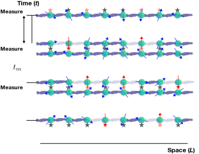
Figure 1: Sketch of the protocol: A quantum spin system, initially frozen in its ground state at quantum criticality ($t=0$), is perturbed with local projective measurements (stars) occurring after every time interval $t_{m}$, with a homogeneous probability $p$ per site. In between two measurement steps, the system evolves unitarily according to its Hamiltonian. Red stars denote the occurrence of a measurement on a given site (for the sake of clarity, in the figure we considered $\sigma^{(3)}$-type measures: spins colored in red are projected along the $z$-axis).

Most of the work done so far in this context focused on the investigation of entanglement transitions genuinely driven by local measurements, either in random circuits LCF-18 ; CNPS-18 ; SRN-18 ; LCF-19 ; SRS-19 ; GH-19 ; BCA-19 ; JYVL-19 ; GH-19-2 ; ZGWGHP-19 , or in the Bose-Hubbard model TZ-19 ; GD-20 , and recently on measurement-induced state preparation RCGG-19 . In noninteracting models, continuous local measurements were shown to largely suppress entanglement CTL-19 . Here we focus on a substantially different dynamic problem: understanding and predicting the effects of local random measurements on the quantum critical dynamics of many-body systems, i.e., when a quantum transition is driven by the Hamiltonian parameters.

Specifically, we consider quantum lattice spin systems, assuming that only one relevant Hamiltonian parameter can deviate from the critical point, which we generically call $\mu$ and assume the critical point to be at $\mu_{c}=0$, with corresponding renormalization-group (RG) dimension $y_{\mu}>0$. The system is initialized, at $t=0$, from the ground state close to the critical point, thus $|\mu|\ll 1$. Random local measurements are then performed at every time interval $t_{m}$, such that each site has a (homogeneous) probability $p$ to be measured. In between two measurement steps, the system evolves according to the unitary operator $e^{-iH(\mu)t}$, as sketched in Fig. 1, where $H(\mu)$ is its Hamiltonian and we fix $\hslash=k_{B}=1$. If $p\to 1$, each spin gets measured every $t_{m}$, and the effects of projections are expected to dominate over those of the unitary evolution. In contrast, for $p$ sufficiently small, the time evolution may result unaffected by the measurements. In between these two regimes, we unveil the existence of a competing unitary vs. projective dynamics, characterized by controllable dynamic scaling behaviors associated with the universality class of the quantum transition.

More complex protocols may be devised. For example, the initial ground state might be replaced with a Gibbs state at a finite temperature $T$. One may also consider a quench of the control parameter at $t=0$, starting from the ground state for a given value $\mu_{0}$ (so that $|\mu_{0}|\ll 1$), to a different value $\mu$ which characterizes the unitary evolution between the measurement steps. In this case, the out-of-equilibrium evolution arises from both the initial quench and the measurement protocol. For the sake of clarity in our presentation, we will focus on the simpler version discussed before, even though an extension to such more complex scenarios is not difficult (see Appendix A).

As for the model, we consider the paradigmatic $d$-dimensional quantum Ising Hamiltonian,

$$H_{\rm Is}=-J\,\sum_{\langle{\bm{x}},{\bm{y}}\rangle}\sigma^{(3)}_{\bm{x}}\sigma^{(3)}_{\bm{y}}-g\,\sum_{\bm{x}}\sigma^{(1)}_{\bm{x}}-h\,\sum_{\bm{x}}\sigma^{(3)}_{\bm{x}}\,,$$ (1)

where ${\bm{\sigma}}\equiv(\sigma^{(1)},\sigma^{(2)},\sigma^{(3)})$ are the spin-1/2 Pauli matrices, the first sum is over the bonds connecting nearest-neighbor sites $\langle{\bm{x}},{\bm{y}}\rangle$, while the other sums are over the sites. We fix $J=1$ as the energy scale. At $g=g_{c}$ and $h=0$, the model undergoes a continuous quantum transition belonging to the two-dimensional Ising universality class, separating a disordered phase ($g>g_{c}$) from an ordered ($g<g_{c}$) one SGCS-97 ; Sachdev-book . Such transition is characterized by a diverging length scale $\xi$ of the critical correlations, and the suppression of the energy gap $\Delta$ as $\Delta\approx\xi^{-z}$, where $z=1$ is the dynamic exponent. The power-law divergence of $\xi$ is related to the RG dimensions of the relevant parameters $\delta\equiv g-g_{c}$ and $h$: it behaves as $\xi\sim|\delta|^{-1/y_{\delta}}$ at $h=0$, and $\xi\sim|h|^{-1/y_{h}}$ for $\delta=0$ Ising1D .

In our dynamic protocol, we take a spin system of linear size $L$ with periodic boundary conditions and perform, on each site, local random measurements of the spin components ${\bm{\sigma}}_{\bm{x}}$, along the transverse [$\sigma_{\bm{x}}^{(1)}$] or the longitudinal [$\sigma_{\bm{x}}^{(3)}$] directions, every time interval $t_{m}$ and with probability $p$. We then project onto the measured value of the spin component, and normalize the many-body wave function. The main features of the resulting evolution are inferred by fixed-time averages of observables, such as magnetization $m(t)$ and susceptibility $\chi(t)$:

$$m(t)=\frac{1}{L^{d}}\sum_{\bm{x}}\langle\sigma_{\bm{x}}^{(3)}\rangle_{t}\,,\quad\chi(t)=\frac{1}{L^{d}}\sum_{{\bm{x}},{\bm{y}}}\langle\sigma_{\bm{x}}^{(3)}\sigma_{\bm{y}}^{(3)}\rangle_{t}\,,$$ (2)

averaging over trajectories ($\langle\cdot\rangle_{t}$ is the expectation value of observables at time $t$). Since measurements generally suppress quantum correlations and $\chi(t\to\infty)\to 1$, corresponding to an uncorrelated state, to monitor this process we study the ratio $R_{\chi}(t)\equiv[\chi(t)-1]/[\chi(t=0)-1]$, which goes from one ($t=0$) to zero ($t\to\infty$). The time scale $\tau_{m}$ of the suppression of quantum correlations may be estimated from the halving time of $R_{\chi}(t)$.

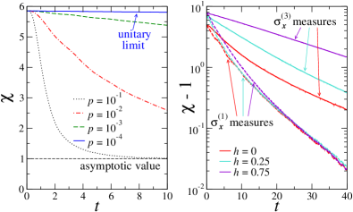
Figure 2: Evolution of the susceptibility $\chi$ for the Ising chain with $L=10$ spins and $g=1$. Local measurements are performed along either the longitudinal direction [$\sigma^{(3)}_{x}$, continuous curves] or the transverse direction [$\sigma^{(1)}_{x}$, dashed curves], with a time interval $t_{m}=0.1$. In the left panel we fix $h=0$ and vary $p$; in the right panel we fix $p=10^{-2}$ and vary $h$, as indicated in the legends. Here and in the next figures data are averaged over many [$O(10^{4})$] trajectories and errors are of the orders of the size of the lines.

As visible from the data in Fig. 2, obtained by numerically simulating the dynamic protocol for a one-dimensional (1D) quantum Ising model Numerics , the random and local spin projections tend to destroy correlations in the system, which converges asymptotically in time to a fully disordered configuration ($\chi=1$, $m=0$). The time scale $\tau_{m}$ of such dynamical process depends on $p$ (left panel), as well as on the initial state and the measurement axis (right panel). In particular, longitudinal-field measurements are less destructive than those along the transverse field, being orthogonal to the coupling and thus to the ordering direction of spins. One can gain more insight on this mechanism, which resembles a relaxation process due to decoherence, by first looking at the exactly solvable single-spin model (see Appendix D, which contains the analytic solution of that model): Irrespective of the magnetic field strength and direction, for finite $t_{m}$, the spin magnetization drops to zero exponentially in time, ending up into a completely unpolarized state. Looking again at the decay highlighted by the curves in Fig. 2, deviations from pure exponentials have thus to be ascribed to the full many-body nature of the system (1).

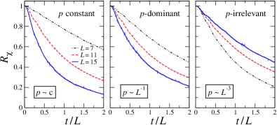
Figure 3: The susceptibility ratio $R_{\chi}$ vs. rescaled time $tL^{-z}$ for the quantum critical Ising chain ($g=1$, $h=0$) for various $L$. Measurements occur along the longitudinal direction, with $t_{m}=0.1$ and $p$ being either constant (left: $c=0.005$) or equal to $p=cL^{-a}$ (middle: $a=1$, $c=0.05$; right: $a=3$, $c=5$). We note that, in the cases $a=0$ and $a=1$, the time scale $\tau_{m}$ of the suppression of the quantum correlations significantly decreases with increasing $L$ as a function of the scaling time $tL^{-z}$; on the other hand it clearly increases for $a=3$.

To achieve a more quantitative understanding of the role of projective measurements in this context, it is worth focusing on the quantum critical region, where universality can be helpful to control the dynamics of the system. Indeed, the out-of-equilibrium critical dynamics at continuous quantum transitions develops homogeneous scaling laws ZDZ-05 ; Dziarmaga-05 ; GZHF-10 ; PSSV-11 ; CEGS-12 ; Ulm-etal-13 ; Biroli-15 ; CC-16 ; PRV-18 ; PRV-18-lo ; NRV-19-wf ; RV-19-de , even in the presence of dissipation YMZ-14 ; NRV-19-dis . One could ask whether similar scaling arguments hold in the above context, as well. A naive application of the dynamic finite-size scaling (FSS) theory Barber-83 ; Privman-90 ; CPV-14 at the critical point of the 1D quantum Ising chain would lead to the results displayed in Fig. 3, where we report the susceptibility ratio $R_{\chi}$ versus the time scaling variable $t/\tau$ where $\tau=L^{z}\sim\Delta^{-1}$ is the time scale of the critical quantum correlations. If the probability $p$ to perform measurements is kept constant while increasing the system size (left panel), the net effect of projections becomes progressively important, eventually overwhelming the unitary Hamiltonian dynamics. Therefore it is clear that a putative scaling behavior could emerge only after a rescaling of $p$ with $L$. Guided by scaling arguments, it is tempting to assume that $p\sim L^{-a}$. Fig. 3 shows that, while with $p\sim L^{-1}$ random measurements are still dominant (middle panel), with $p\sim L^{-3}$ they become irrelevant for the asymptotic dynamic scaling (right panel). In between these two cases, there could be a suitable power-law exponent entering the proper scaling theory for the dynamics arising from the random measurement protocol described above, provided this is possible.

Taking advantage of the previous insight, we put forward a phenomenological scaling theory in which, as working hypothesis, we assume a scaling behavior for the parameters $t_{m}$ and $p$ characterizing the measurement procedure. We conjecture that a generic observable $B$ (averaged over the trajectories) follows the scaling law

$$B(\mu,t,t_{m},p)\approx b^{-y_{B}}{\cal B}(\mu b^{y_{\mu}},tb^{-z},t_{m}\,b^{\zeta},pb^{\varepsilon})\,.$$ (3)

Here $b$ denotes an arbitrary positive parameter, $y_{B}$ is the critical RG dimension of the operator $B$, while $\zeta$ and $\varepsilon$ are appropriate exponents associated with the measurement process, and ${\cal B}$ is a universal scaling function apart from normalizations (more details are provided in Appendix A). Equation (3) is expected to provide the power-law asymptotic behavior in the large-$b$ limit, neglecting further dependences on other parameters, which are supposed to be suppressed (and thus irrelevant) in such limit.

The arbitrariness of the scale parameter $b$ in Eq. (3) can be fixed by setting $b=\lambda\equiv|\mu|^{-1/y_{\mu}}$, where $\lambda\sim\xi$ is the length scale of the critical modes. The scaling variable associated with the time interval $t_{m}$ should be given by the ratio $t_{m}/\tau$, where $\tau\sim\Delta^{-1}\sim\lambda^{z}$ is the time scale of the critical models (this implies $\zeta=-z$). Keeping $t_{m}$ fixed in the large-$\lambda$ limit, the dependence on $t_{m}$ disappears asymptotically, giving only rise to $O(\lambda^{-z})$ scaling corrections. Moreover, noticing that the parameter $p$ is effectively a probability per unit of time and space, a reasonable guess would be that its correct scaling to compete with the critical modes is that $p\sim\lambda^{-z-d}$, thus

$$\varepsilon=z+d\,.$$ (4)

This leads to the dynamic scaling equation $B(\mu,t,t_{m},p)\approx\lambda^{-y_{B}}{\cal B}(t\lambda^{-z},p\lambda^{\varepsilon})$ footnotesiB . We stress that the value of the exponent $\varepsilon$ in Eq. (4) is crucial, because it allows to separate the measurement-irrelevant regime $p=o(\lambda^{-\varepsilon})$ (right panel of Fig. 3) from the measurement-dominant regime $p\lambda^{\varepsilon}\to\infty$ (left and middle panels of Fig. 3). Note that, since $p\sim\lambda^{-\varepsilon}$ and $t\sim\lambda^{z}$, the dynamic scaling ansatz predicts that the time scale $\tau_{m}$ associated with the suppression of the quantum correlations behaves as $\tau_{m}\sim p^{-\kappa}$ with $\kappa=z/\varepsilon<1$.

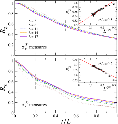
Figure 4: Time behavior of $R_{\chi}$ at criticality, for various sizes. Random measurements are either along the longitudinal (upper plots) or the transverse direction (lower plots), for $t_{m}=0.1$, $p=1/L^{2}$ according to the scaling (4). Data converge to an asymptotic scaling function, as also shown by the two insets, displaying data for a specific value of $t/L$ (dashed line in the main frames). They are compatible with a $O(L^{-3/4})$ approach to the asymptotic behavior (dashed red lines). Analogous scaling results are obtained for $t_{m}\to 0$, as shown in Appendix C.

The above scaling theory holds in the thermodynamic limit $L/\lambda\to\infty$, that is expected to be well defined for any $\mu\neq 0$, for which $\lambda$ is finite. Nonetheless, for most practical purposes, both experimental and numerical, one typically has to face with systems of finite length. Such situations can be framed in the FSS framework, where the scale parameter in Eq. (3) is fixed to $b=L$ Barber-83 ; Privman-90 ; CPV-14 ; SGCS-97 ; CNPV-14 ; PRV-18 . Assuming again that $t_{m}$ is kept fixed, straightforward manipulations lead to the following scaling law

$$B(\mu,t,t_{m},p,L)\approx L^{-y_{B}}{\cal B}(\mu L^{y_{\mu}},tL^{-z},pL^{\varepsilon})\,.$$ (5)

The proper dynamic FSS behavior is obtained by taking $L\to\infty$, while keeping $t_{m}$ and the arguments of the scaling function ${\cal B}$ fixed.

It is worth mentioning that analogous scaling ansatzes for more general observables, such as fixed-time correlation functions of two operators, can be obtained using the same arguments and assumptions (see Appendix A). They can be extended to include an initial quench of the Hamiltonian parameter $\mu_{0}\to\mu$ [by adding a further dependence on $\mu_{0}b^{y_{\mu}}$ in Eq. (3)], to consider finite-temperature initial Gibbs states (by adding a dependence on $Tb^{z}$), and allowing for weak dissipation NRV-19-dis . We note that the scaling arguments do not depend on the type of local measurement, therefore they are expected to be somehow independent of them. Further investigations are called for to classify the extension of such independence.

The above phenomenological scaling theory has been checked on the quantum Ising chain. The dynamic FSS laws for the magnetization $m$ and its susceptibility $\chi$ follow Eq. (5), in which the parameter $\mu$ corresponds to either $\delta=g-g_{c}$ or $h$ in Eq. (1). In particular, for $\delta=h=0$, one obtains $m(t)=0$ by symmetry, and

$$R_{\chi}(t,t_{m},p,L)\equiv\frac{\chi(t)-1}{\chi(t=0)-1}\approx{\cal R}_{\chi}(tL^{-z},pL^{\varepsilon})\,.$$ (6)

Further details are provided in Appendix B. Results for a system at the quantum critical point, with random local longitudinal and transverse spin measurements, are shown in Fig. 4. The data of $R_{\chi}$ versus $tL^{-z}$ nicely agree with Eq. (6). Corrections to the scaling are consistent with a $L^{-3/4}$ approach, as expected (see the insets). An analogous agreement has been obtained for the magnetization at $h\neq 0$, keeping $hL^{y_{h}}$ constant (see Appendix C).

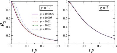
Figure 5: $R_{\chi}$ for the quantum Ising chain with $L=10$ spins, $h=0$, as a function of $t\,p$. Local measurements are performed along $\sigma^{(3)}_{x}$, with $t_{m}=0.1$ and varying $p$ (see legend). We fix $g=1.1$ (left) or $g=2$ (right). The approximate collapse of the data versus $t\,p$ indicates that, in these two cases with $g>g_{c}$, the characteristic time $\tau_{m}$ scales as $\tau_{m}\sim p^{-1}$.

We finally focus on systems which are not close to a phase transition (for example, $g>g_{c}$ in the case of quantum Ising models). In this case, the system lies in the disordered phase, where the length scale $\xi$ of the quantum correlations and the gap $\Delta$ remain finite with increasing $L$. The data reported in Fig. 5 for $R_{\chi}$ at fixed size $L$ suggest that, away from criticality, the characteristic time $\tau_{m}$ of the measurement process scales as $\tau_{m}\sim p^{-1}$, unlike the critical behavior, where $\tau_{m}\sim p^{-\kappa}$ with $\kappa=z/\varepsilon<1$.

Summarizing, we showed the emergence of different dynamic regimes arising from the interplay between unitary and projective dynamics in many-body systems at quantum transitions, where quantum correlations develop a diverging length scale. One of them is characterized by the dominance of the local random measurements, for example for any finite probability $p$ of making the local measurement. In contrast, for sufficiently small values of $p$ (i.e. decreasing as a sufficiently large power of the inverse diverging length scale $\xi$), the measurements turn out to be irrelevant. We conjectured these two regimes to be separated by dynamic conditions imposing suitable scaling behaviors for the characterizing parameters of the protocol, such as the local measurement probability $p$, which is controlled by the universality class of the quantum transition. For a $d$-dimensional critical system, this occurs when $p\sim\xi^{-\varepsilon}$, for which we argue $\varepsilon=z+d$, where $z$ is the dynamic exponent of the transition.

This general scenario is supported by numerical results for the quantum Ising chain, for protocols involving the measurements of either transverse or longitudinal component of the local spin operator. Local measurements generally tend to suppress quantum correlations, even in the dynamic scaling limit. The corresponding time scale is expected to behave as $\tau_{m}\sim p^{-\kappa}$ with $\kappa=z/\varepsilon<1$, to be compared with the noncritical case $\tau_{m}\sim p^{-1}$. The smaller power $\kappa$ at the critical point can be explained by the fact that the relevant probability ($p_{r}$) driving the measurement process is the probability to perform a local measurement within the critical volume $\xi^{d}$, therefore $p_{r}=p\,\xi^{d}$. The time rate thus behaves as $\tau_{m}\sim p_{r}^{-1}$, similarly to the noncritical case, where $\xi=O(1)$.

Additional checks are called for, in order to achieve a definite validation of our scaling conjectures, such as the study of protocols with quenches of the Hamiltonian parameters, higher dimensions, other quantum transitions (in particular characterized by different values of the dynamic exponent $z$) and measurement schemes (non necessarily strictly onsite, but still sufficiently local). Furthermore we expect that arguments similar to those employed here could be used for measurements that are localized in restricted regions of space, and also to derive possible peculiar scaling phenomena in proximity of first-order quantum transitions, where the boundary conditions could play a more relevant role PRV-18 ; PRV-18-bc .

Given the relatively small sizes required to reach the scaling limit, a direct experimental realization of our protocol can be reasonably considered as a near-future target for quantum simulations. Promising platforms are superconducting quantum circuits Barends-15 ; Harris-18 ; Minev-etal-19 , nuclear spins Jiang-etal-09 ; KCTMHT-16 , trapped ions Zhang-17 ; NMMFH-18 ; Brydges-19 and ultracold atomic systems BGPFG-09 ; SWECBK-10 ; PCV-15 ; Bernien-17 .

Appendix A Phenomenological scaling theory of the out-of-equilibrium dynamics induced by local measurements

We work out a phenomenological scaling theory for the out-of-equilibrium dynamics arising from random local projective measurements during the evolution of a many-body system at a quantum transition Sachdev-book . For simplicity, we assume that the quantum transition is driven by a relevant parameter $\mu$ of the Hamiltonian $H(\mu)$, whose critical value is $\mu_{c}=0$. At the critical point, the low-energy unitary Hamiltonian dynamics develops long-distance correlations, characterized by a diverging length scale $\xi\sim|\mu|^{-\nu}$, where $\nu=1/y_{\mu}$ and $y_{\mu}$ is the renormalization-group (RG) dimension of the relevant parameter.

More specifically, we consider the dynamic problem associated with the following protocol: (a) The system starts at $t=0$ from the ground state close to the critical point, thus $|\mu|\ll 1$; (b) Random local measurements are performed every time interval $t_{m}$, with a homogeneous probability $p$ per site. Between two measurement steps, the system evolution is driven by the unitary operator $e^{-iH(\mu)t}$. Hereafter we adopt units of $\hslash=k_{B}=1$.

The out-of-equilibrium critical dynamics at continuous quantum transitions has been shown to obey homogeneous scaling laws ZDZ-05 ; Dziarmaga-05 ; GZHF-10 ; PSSV-11 ; CEGS-12 ; Ulm-etal-13 ; Biroli-15 ; CC-16 ; PRV-18 ; PRV-18-lo ; NRV-19-wf ; RV-19-de , even in the presence of dissipation YMZ-14 ; NRV-19-dis . For example, after an instantaneous quench from $\mu_{0}=0$ to $\mu$, a generic observable $B$ at fixed time $t$ after the quench, is generally expected to behave as PRV-18

$$B(\mu,t,L)\approx b^{-y_{B}}{\cal B}(\mu b^{y_{\mu}},tb^{-z},L/b)\,,$$ (7)

where $b$ is an arbitrary positive parameter, $L$ is the linear size of the $d$-dimensional system under investigation, and ${\cal B}$ is a universal scaling function apart from normalizations. The exponent $y_{B}$ denotes the RG dimension of the operator associated to $B$, while the dynamic exponent $z$ characterizes the behavior of the energy differences of the lowest-energy states and, in particular, the ground-state gap $\Delta\sim L^{-z}$. Equation (7) is expected to provide the asymptotic power-law behavior in the large-$b$ limit.

We now extend the dynamic scaling arguments leading to Eq. (7), by allowing for the dependence on the parameters $t_{m}$ and $p$ which characterize the measurement procedure of the protocol. As a working hypothesis, we assume that an asymptotic scaling behavior is achieved by appropriately rescaling $t_{m}$ and $p$, such as

$$B(\mu,t,t_{m},p,L)\approx b^{-y_{B}}{\cal B}(\mu b^{y_{\mu}},tb^{-z},t_{m}\,b^{\zeta},pb^{\varepsilon},L/b),\quad$$ (8)

where $\zeta$ and $\varepsilon$ are appropriate exponents whose relevance is discussed below.

A.1 Dynamic finite-size scaling

It is possible to exploit the arbitrariness of the scale parameter $b$. For example, by setting $b=L$, we obtain the dynamic finite-size scaling (FSS) equations, extending those holding for closed systems SGCS-97 ; CPV-14 ; CNPV-14 ; PRV-18 . Analogously as for the time $t$ that has passed after the quench, the scaling variable associated with the time interval $t_{m}$ should be given by the ratio $t_{m}/\tau$ where $\tau\sim\Delta^{-1}\sim L^{z}$ is the time scale of the critical models, thus

$$\zeta=-z\,.$$ (9)

If one keeps $t_{m}$ fixed in the large-$L$ dynamic FSS limit, the dependence on $t_{m}$ disappears asymptotically, giving only rise to $O(L^{-z})$ scaling corrections. Moreover, noting that the parameter $p$ is effectively a probability per unit of time and space, a reasonable guess is that we must have the power-law scaling behavior $p\sim L^{-z-d}$ to achieve a nontrivial competition with the critical modes. Therefore,

$$\varepsilon=z+d\,.$$ (10)

We stress that the value of the exponent $\varepsilon$ is crucial, because it allows us to separate the regime $p=o(L^{-\varepsilon})$ in which the random measurements are irrelevant for the asymptotic dynamic scaling, from that where they drive the evolution overwhelming the unitary Hamiltonian dynamics, when $pL^{\varepsilon}\to\infty$.

On the basis of these scaling arguments, from Eq. (8) we conjecture that, keeping $t_{m}$ and the arguments of the scaling function ${\cal B}$ fixed, the dynamic FSS law associated with the random-measurement protocol reads

$$B(\mu,t,t_{m},p,L)\approx L^{-y_{B}}{\cal B}(\mu L^{y_{\mu}},tL^{-z},pL^{\varepsilon})\,.$$ (11)

The scaling function ${\cal B}$ is expected to be largely universal with respect to the Hamiltonian of the system, within a given universality class, and also with respect to the details of the protocol. Of course, like any scaling function a quantum transition, such universality is expected modulo a multiplicative overall constant and normalizations of the scaling variables. Note that, in this case, the asymptotic scaling behavior does not depend on $t_{m}$ and therefore it is expected to hold also in the limit $t_{m}\to 0$.

Alternatively, one may rescale the time interval $t_{m}$ as $\tau\sim L^{z}$, thus keeping the ratio $t_{m}/L^{z}$ fixed. In this case we expect the probability $p$ to scale as the inverse volume only, i.e.

$$B(\mu,t,t_{m},p,L)\approx L^{-y_{B}}{\cal B}(\mu L^{y_{\mu}},tL^{-z},t_{m}L^{-z},pL^{d})\,.$$ (12)

Note that, analogously to Eq. (11), the FSS limit requires that $p/t_{m}\sim L^{-\varepsilon}$. Similar scaling ansatzes for more general observables, such as fixed-time correlation functions of two operators, can be straightforwardly obtained using the same assumptions and scaling arguments.

The above predictions can be extended to the more complex protocol including an initial quench of the Hamiltonian parameter from $\mu_{0}$ to $\mu$; this is achieved by adding the further dependence on $\mu_{0}L^{y_{\mu}}$. Moreover, one may also consider an initial Gibbs state for a small temperature $T$, and this can be taken into account by adding a further scaling variables $TL^{z}$.

We finally note that our scaling arguments do not apparently depend on the type of local measurement, thus they are expected to be somehow independent on them.

A.2 Dynamic scaling in the thermodynamic limit

To derive a dynamic scaling theory for infinite-volume systems, we may restart from the general homogeneous power law in Eq. (8) and set

$$b=\lambda\equiv|\mu|^{1/y_{\mu}}\,,$$ (13)

where $\lambda$ is the length scale of the critical modes, and consider the limit $L/\lambda\to\infty$, assuming that it is well defined (this limit corresponds to the so-called thermodynamic limit, which is expected to be well defined for any $\mu\neq 0$, for which $\lambda$ is finite). Then, keeping again $t_{m}$ fixed such that $t_{m}/\lambda^{z}\to 0$ in the $\lambda\to\infty$ limit, and using the fact that the power law associated with $p$ is expected to be characterized by the same exponent $\varepsilon$ given in Eq. (10), one obtains the dynamic scaling ansatz

$$B(\mu,t,t_{m},p)\approx\lambda^{-y_{B}}{\cal B}(t\lambda^{-z},p\lambda^{\varepsilon})\,,$$ (14)

where $\varepsilon=z+d$ is given as in Eq. (10). Note that, strictly speaking, one has two scaling functions ${\cal B}$, depending on the sign of $\mu$.

Appendix B Dynamic scaling within the quantum Ising model

The one-dimensional (1D) quantum Ising model in a transverse field is one of the simplest paradigmatic quantum many-body systems exhibiting a nontrivial zero-temperature phase diagram. The corresponding Hamiltonian reads

$$H_{\rm Is}=-J\,\sum_{x}\sigma^{(3)}_{x}\sigma^{(3)}_{x+1}-g\,\sum_{x}\sigma^{(1)}_{x}-h\,\sum_{x}\sigma^{(3)}_{x}\,,$$ (15)

where ${\bm{\sigma}}\equiv(\sigma^{(1)},\sigma^{(2)},\sigma^{(3)})$ are the spin-1/2 Pauli matrices, the first sum is over all bonds of the chain connecting nearest-neighbor sites, while the other sums are over the sites of the chain. In our numerical studies, we set $J=1$ as the energy scale and consider chains of size $L$ with periodic boundary conditions (${\bm{\sigma}}_{L+1}\equiv{\bm{\sigma}}_{1}$).

At $g=g_{c}$ and $h=0$ (in 1D, $g_{c}=1$), the model undergoes a continuous quantum transition belonging to the two-dimensional Ising universality class, separating a disordered phase ($g>1$) from an ordered ($g<1$) one (see e.g. Refs. SGCS-97 ; Sachdev-book ). Such transition is characterized by a diverging length scale $\xi$ of the critical correlations and the suppression of the ground-state energy gap $\Delta$ as $\Delta\approx\xi^{-z}$ with $z=1$. The power-law divergence of $\xi$ is related to the RG dimensions, $y_{\delta}$ and $y_{h}$, of the relevant parameters $\delta\equiv g-g_{c}$ and $h$, respectively. For the transverse field it is given by

$$y_{\delta}=1/\nu\,,$$ (16)

while for the longitudinal field

$$y_{h}=\tfrac{1}{2}\big{(}d+z+2-\eta\big{)}\,,$$ (17)

$\eta$ being the exponent which describes the critical behavior of the correlation function of the order parameter $\sigma^{(3)}$. Therefore, the critical length scale diverges as $\xi\sim|\delta|^{-1/y_{\delta}}$ for $h=0$, and $\xi\sim|h|^{-1/y_{h}}$ for $\delta=0$. Specializing to the 1D case, one has $d=1$, $\nu=1$, and $\eta=1/4$, therefore $y_{\delta}=1$ and $y_{h}=15/8$ CPV-14 .

For dynamic protocols using the quantum Ising Hamiltonian in Eq. (15), the evolution of the system can be effectively characterized by the time dependent magnetization along the coupling direction

$$M(t)=\frac{1}{L}\sum_{x}\langle\sigma_{x}^{(3)}\rangle_{t}\,,$$ (18a)

the fixed-time longitudinal correlation function

$$G(x,y,t)=\langle\sigma_{x}^{(3)}\sigma_{y}^{(3)}\rangle_{t}\,,$$ (18b)

and the corresponding susceptibility

$$\chi(t)=\frac{1}{L}\sum_{x,y}G(x,y,t)\,.$$ (18c)

Here $\langle\cdot\rangle_{t}$ indicates the expectation value of a given observable at time $t$. Note that translation invariance, which also applies in finite-size systems with periodic boundary conditions, implies $G(x,y,t)\equiv G(x-y,t)$.

For the sake of presentation and without loss of generality, we fix $g=g_{c}$ and only vary $h$, so that $h$ corresponds to the parameter $\mu$ of the above-reported scaling equations (analogous equations would hold if $g$ were varied, with the substitution $h\to\delta$ and $y_{h}\to y_{\delta}$). The dynamic FSS laws of the observables (18a)-(18c), keeping $t_{m}$ fixed, thus read

$$M(h,t,t_{m},p,L)\! \!\approx\!\! \!L^{-{y_{m}}}\,{\cal M}(hL^{y_{h}},tL^{-z},pL^{\varepsilon}),\qquad\;\;$$ (19a)

$$G(x,h,t,t_{m},p,L)\! \!\approx\!\! \!L^{-{2y_{m}}}\,{\cal G}(\tfrac{x}{L},hL^{y_{h}},tL^{-z},pL^{\varepsilon}),\qquad\;\;$$ (19b)

$$\chi(h,t,t_{m},p,L)\! \!\approx\!\! \!L^{d-2y_{m}}\,{\cal C}(hL^{y_{h}},tL^{-z},pL^{\varepsilon}),\qquad\;\;$$ (19c)

where $y_{m}$ is the RG dimension of the longitudinal spin operator $\sigma_{x}^{(3)}$, given by

$$y_{m}=\tfrac{1}{2}\big{(}d+z-2+\eta\big{)}\,,$$ (20)

and the power of the prefactor associated with the longitudinal spin correlation (18b) is twice $y_{m}$ ($y_{m}=1/8$, in 1D). In particular, for $h=0$ one has $M(t)=0$ and

$$\chi(t,t_{m},p,L)\approx L^{d-2y_{m}}\,{\cal C}_{c}(tL^{-z},pL^{\varepsilon})\,.$$ (21)

Corrections to scaling are generally expected to be $O(1/L)$, see for example Refs. CPV-14 ; PRV-18 ; RV-19-de . However we note that, in the case of the susceptibility $\chi$ defined as in Eq. (18c), $O(L^{-d+2y_{m}})$ corrections are also present, already at the level of the equilibrium ground-state values of $\chi$, due to analytic contributions to the critical behavior, as explained in Ref. CPV-14 . Therefore, in the case of the Ising chain, we expect that the leading scaling corrections to the asymptotic dynamic scaling of the evolution of $\chi$ are $O(L^{-3/4})$.

Our numerical results show that the measurement process generally tends to suppress quantum correlations, therefore $\chi(t)$ is a monotonic decreasing function. In particular, the numerics provides evidence of the fact that

$$\lim_{t\to\infty}\chi(t)=1\,.$$ (22)

The asymptotic value corresponds to a fully disordered state with vanishing correlations, $G(x,\,y,\,t\!\to\!\infty)=0$ (for $x\neq y$), and where the only non-zero contributions entering the sum (18c) are those for $x=y$, which trivially sum up to one. To monitor the suppression of quantum correlations due to the measurement process, it is thus convenient to introduce the ratio

$$R_{\chi}=\frac{\chi(t)-1}{\chi(t=0)-1}\,,$$ (23)

which goes from one (for $t=0$) to zero (for $t\to\infty$). In the dynamic scaling limit at the critical point, using Eq. (21), we can immediately derive the asymptotic behavior

$$R_{\chi}(t,t_{m},p,L)\approx{\cal R}_{\chi}(tL^{-z},pL^{\varepsilon})\,.$$ (24)

Note that, in the dynamic scaling limit, $R_{\chi}\approx\chi(t)/\chi(0)$, i.e. the finite subtraction of one in the numerator and denominator of the definition of $R_{\chi}$ turns out to be irrelevant. Therefore, like for the susceptibility, the approach to the asymptotic dynamic FSS behavior (24) is expected to be characterized by $O(L^{-3/4})$ corrections for the quantum Ising chain (see results reported in Fig. 4).

In the infinite-volume limit, at $g=g_{c}$, we expect to have

$$M(h,t,t_{m},p) \approx \lambda^{-y_{m}}\,{\cal M}(t\lambda^{-z},p\lambda^{\varepsilon})\,,\quad$$ (25a)

$$G(x,h,t,t_{m},p) \approx \lambda^{-2y_{m}}\,{\cal G}(x/\lambda,t\lambda^{-z},p\lambda^{\varepsilon})\,,\quad$$ (25b)

$$\chi(h,t,t_{m},p) \approx \lambda^{d-2y_{m}}\,{\cal C}(t\lambda^{-z},p\lambda^{\varepsilon})\,,\quad$$ (25c)

where $\lambda=|h|^{-1/y_{h}}$. Such dynamic scaling behaviors are expected to be approached asymptotically for $L\to\infty$, keeping fixed the scaling variables of the functions ${\cal M}$ and ${\cal C}$.

As already noted above, the dynamic scaling arguments that we have outlined do not apparently depend on the type of local measurement. In particular, in the case of the quantum Ising model, they should apply to protocols based on both $\sigma_{\bm{x}}^{(1)}$ or $\sigma_{\bm{x}}^{(3)}$ local measurements.

The time scale $\tau_{m}$ of the suppression of the quantum correlations may be estimated from the halving time of $R_{\chi}(t)$. Its power-law scaling behavior in terms of the probability $p$ can be easily derived in the dynamic scaling limit, by noting that $p\sim\xi^{-\varepsilon}$ and $t\sim\xi^{z}$ where $\xi$ is the length scale of the critical modes (that is $\xi\sim L$ at the critical point and $\xi\sim\lambda$ around it). Therefore, the dynamic scaling predicts that the time scale $\tau_{m}$ associated with the suppression of the quantum correlations behaves as

$$\tau_{m}\sim p^{-\kappa}\,,\qquad\kappa=\frac{z}{\varepsilon}=\frac{z}{z+d}\,.$$ (26)

Note that $\kappa<1$, thus the time rate in terms of $p$ turns out to be accelerated with respect the noncritical behavior $\tau_{m}\sim p^{-1}$ which has been obtained numerically, see Fig. 5. This apparently counterintuitive behavior can be explained by the nontrivial fact that the relevant probability $p_{r}$, which drives the measurement process, is the probability to perform a local measurement within the critical volume $\xi^{d}$, therefore $p_{r}=p\,\xi^{d}$. In terms of $p_{r}$, the time rate thus behaves as

$$\tau_{m}\sim p_{r}^{-1}\,,\qquad p_{r}=p\,\xi^{d}\,,$$ (27)

similarly to the noncritical case, where $\xi=O(1)$.

Appendix C Some details on the numerical computations

To check our phenomenological dynamic scaling theory discussed before, we have performed some numerical simulations on the 1D quantum Ising chain (15), based on exact diagonalization (ED). We are interested in the random-measurement protocol starting from the ground state of a system of size $L$ (with periodic boundary conditions) for the Hamiltonian parameter $h$ and with $g=g_{c}=1$, which has been obtained by means of a Lanczos technique. The evolution, monitored through a fourth-order Suzuki-Trotter decomposition of the unitary-evolution operator with time step $dt=0.005$, is essentially driven by the random measurements, which are performed at every time interval $t_{m}$. We have considered either local longitudinal [$\sigma_{x}^{(3)}$] or transverse [$\sigma_{x}^{(1)}$] measurements, occurring with a probability $p$ per site.

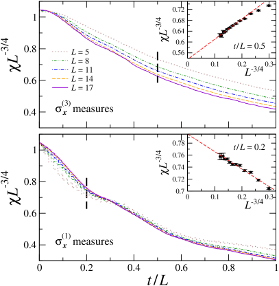
Figure 6: Rescaled susceptibility $\chi L^{-3/4}$ at criticality ($g=1$, $h=0$), as a function of the rescaled time $t/L$, for the quantum Ising chain with different system sizes $L$ (see legend). The upper frame refers to random measures along the longitudinal direction [$\sigma^{(3)}_{x}$], while the lower frame refers to random measures along the transverse direction [$\sigma^{(1)}_{x}$]. Measurements are characterized by $t_{m}=0.1$, $p=1/L^{2}$ as predicted by Eq. (10). The two insets display the same data of the main panels for a specific cut in the rescaled time ($t/L=0.5$ for the upper frame, $t/L=0.2$ for the lower frame) versus $L^{-3/4}$. The approach to the asymptotic value is consistent with the expected $O(L^{-3/4})$ corrections. Dashed red lines denote $1/L^{3/4}$ fits to numerical data (black circles) and have been obtained by discarding points for the smaller available sizes. Here and in the next figures, data have been averaged over a number of $N_{\rm avg}=2\times 10^{3}$ (for $L\leq 14$) and $N_{\rm avg}=2\times 10^{3}$ (for $L\geq 15$) trajectories.

In Fig. 4 we showed results only for the susceptibility ratio $R_{\chi}$. Here we provide some additional data, both for the magnetization (18a) and for the susceptibility (18c), in which we kept $g=1$ and varied the longitudinal field $h$ (note that the quantum Ising chain with $h\neq 0$ is not integrable).

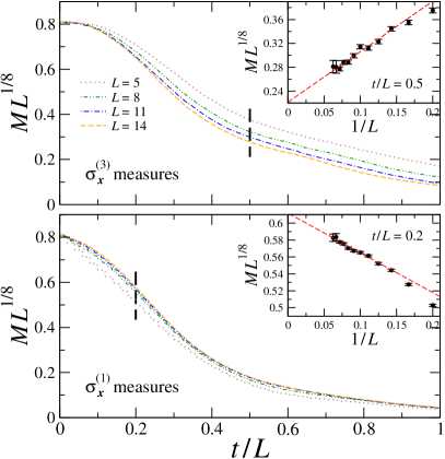
Figure 7: Same as in Fig. 6, but for the rescaled magnetization $ML^{1/8}$ vs. the rescaled time $t/L$. The initial state here is the ground state of the quantum Ising ring with $g=1$ and rescaled longitudinal field $hL^{15/8}=1$, which has a finite magnetization. The two insets display the same data of the main panels for a specific cut in the rescaled time, versus $1/L$. The approach to the asymptotic FSS behavior, for finite $L$, appears to be consistent with the expected $O(1/L)$ trend (dashed red lines).

The need of averaging over many different trajectories, typically $O(10^{4})$, together with the fact that the numerical results shown in this paper are nicely consistent with the dynamic FSS theory, prevented us from studying systems with more than $L=18$ sites, although larger sizes would be easily addressable for a single trajectory or a few ones. Also note that we preferred to use conventional (and fully controllable) ED techniques over DMRG-based algorithms Schollwock-11 ; Daley-14 , since with those latter methods it is more complicated to guarantee the required accuracy in order to carefully test our phenomenological scaling theory. Nonetheless, there are no conceptual limitations in using DMRG for analyzing the measurement-induced dynamics of quantum lattice models with finite degrees of freedom TZ-19 . In summary, ED techniques are more controllable, but suffer from severe limitations in the reachable system sizes; DMRG allows to study larger systems, although it requires more care in the choice of the bond-link dimension for the study of dynamical problems.

Figure 6 displays the numerical outcomes for the susceptibility at the Ising critical point ($g=1$, $h=0$), for random local measurements taken along the longitudinal or the transverse direction. Note that the results presented in this figure are the same as those reported in Fig. 4, but for the rescaled susceptibility $\chi\,L^{-3/4}$ [instead of the ratio $R_{\chi}$ in Eq. (23)]. Similarly as for the susceptibility ratio, we observe a nice agreement with the predicted scaling behavior in Eq. (19c). Moreover, corrections to the scaling are consistent with a $L^{-3/4}$ behavior, as expected (see the two insets).

Results for the magnetization $m(t)$ are reported in Fig. 7. In that case, we considered $g=1$ and a nonzero longitudinal field $h$, since the latter is essential in order to start from an initially magnetized state [$m(0)\neq 0$]. After a suitable rescaling of all the relevant parameters, the various curves approach an asymptotic scaling behavior, as indicated in Eq. (19a). Notice that we also rescaled the field $h$ so to keep the scaling variable $hL^{15/8}$ constant. The approach to the scaling is governed by corrections whose leading order appear to be consistent with a $L^{-1}$ behavior, as witnessed by the two insets.

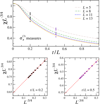
Figure 8: Same as in Fig. 6, but for random local measurements along the longitudinal direction in the continuous time limit $t_{m}\to 0$ and with $p=0.1/L^{2}$. The lower panels display the same data of the main panel, for two specific values of rescaled time (left: $t/L=0.2$; right: $t/L=0.5$) versus $L^{-3/4}$. The approach to the asymptotic value is consistent with the expected $L^{-3/4}$ corrections (dashed red lines).

All the numerical data presented above correspond to fixing the time interval between two consecutive measurements equal to $t_{m}=0.1$. We have checked that analogous scaling results can be obtained for arbitrary values of $t_{m}$. In particular, in Fig. 8 we have considered the limit $t_{m}\to 0$. More precisely, random local measurements have been performed at every Trotter time step, so that $t_{m}=0.005$. The upper panel displays results for the rescaled susceptibility $\chi L^{-3/4}$ as a function of the rescaled time $t/L$, keeping $g=1$ and $h=0$, for measurements performed along the longitudinal direction [$\sigma_{x}^{(3)}$]. The lower panels highlight that corrections to the scaling are $O(L^{-3/4})$, as expected. Notice that here the compatibility with a $L^{-3/4}$ behavior (dashed red lines) is excellent already at very small system sizes ($L=5$), contrary to the case of larger $t_{m}$ values: compare with the insets of Fig. 6, where deviations from the expected trend emerge at smaller $L$. This hints at the fact that other subleading terms, that may enter the scaling corrections at finite $L$, may get suppressed in the limit $t_{m}\to 0$, such as those which are $O(t_{m}/L^{z})$.

Finally we observe that the same scaling functions (${\cal M}$, ${\cal G}$, ${\cal C}$, …) are expected to hold for vanishing $t_{m}$, so that the asymptotic curves for the magnetization and the susceptibility at $L\to\infty$ should coincide with those at finite $t_{m}$, after a proper rescaling of all the relevant parameters in the dynamic protocol.

Appendix D One-spin model subject to periodic measurements

Here we discuss the dynamics of a single spin-$1/2$ system in a magnetic field, subject to periodic measurements along a given axis, for which it is possible to derive an analytic solution. We consider the following Hamiltonian model:

$$H_{1}=-g\,\sigma^{(1)}-h\,\sigma^{(3)}\,,$$ (28)

where $g$ and $h$ denote the intensity of an applied external magnetic field along two orthogonal directions [${\bm{\sigma}}\equiv(\sigma^{(1)},\sigma^{(2)},\sigma^{(3)})$ are the usual spin-1/2 Pauli matrices]. Without loss of generality, we fix $g=1$. We now suppose to initialize the system in its ground state, associated with the parameter $h$ at $t=0$. Then we perform a sequence of repeated measurements of the operator $\sigma^{(3)}$ at every time interval $t_{m}$ (the choice of the measurement axis is arbitrary).

The dynamics arising from this protocol can be described in terms of the system’s density matrix $\rho$. The starting ($t=0$) state is a pure state, given by

$$\rho_{0}\equiv\rho(t=0)=|0_{h}\rangle\langle 0_{h}|\,,$$ (29)

where

$$E_{0} = -\sqrt{1+h^{2}}\,,$$ (30)

$$|0_{h}\rangle = {\cal N}\left[(-h-\sqrt{1+h^{2}})|+\rangle+|-\rangle\right]\,,$$ (31)

and $|\pm\rangle$ are the eigenstates of $\sigma^{(3)}$, while ${\cal N}$ is the normalization to obtain $\langle 0_{h}|0_{h}\rangle=1$. Then, defining the density matrix after $n$ measurements, at time $t=nt_{m}$, as

$$\rho_{n}\equiv\rho(t=nt_{m})\,,$$ (32)

the subsequent dynamics can be described as a series of two-step operations:
(i) A unitary time evolution for a time $t_{m}$,

$$\tilde{\rho}_{n+1}=e^{-iH_{1}t_{m}}\rho_{n}e^{iH_{1}t_{m}}\,;$$ (33a)

(ii) The measurement of $$\sigma^{(3)}$$,

$$\rho_{n+1}={\rm Tr}(\tilde{\rho}_{n+1}P_{+})\,P_{+}+{\rm Tr}(\tilde{\rho}_{n+1}P_{-})\,P_{-}\,,$$ (33b)

where $$P_{\pm} |\pm\rangle \sigma^{(3)}$$ are the projectors onto the eigenstates of . Simple manipulations thus lead to

$$\rho_{n+1}=\tfrac{1}{2}I+W_{n+1}\sigma^{(3)},\qquad W_{n+1}=\tilde{\rho}_{n+1}^{11}-\tfrac{1}{2}\,,$$ (33c)

where $W$ quantifies the deviation from the trivial completely unpolarized density matrix $\rho_{u}=I/2$. Given the initial condition (29), one finds

$$W_{1}=\frac{h(\sqrt{1+h^{2}}+h)}{2(1+h^{2}+h\sqrt{1+h^{2}})}\,.$$ (34)

Straightforward computations allow to obtain

$$W_{n+1}=f\,W_{n}\,,\qquad f=1-\frac{2[\sin(t_{m}\sqrt{1+h^{2}})]^{2}}{1+h^{2}}\,.$$ (35)

In particular, for $h=1$, one gets $W_{1}=(1+\sqrt{2})/(4+2\sqrt{2})\approx 0.35355$ and $f=1-\sin^{2}(\sqrt{2}t_{m})$. Note that the factor $f$ is bounded, indeed

$$|f|\leq 1\,.$$ (36)

Moreover, for arbitrary values of $h$ and $t_{m}$, one strictly finds $|f|<1$. Indeed $f=-1$ for $h=0$ only, while $f=1$ for the specific values $t_{m}=m\pi/\sqrt{1+k^{2}}$, with integer $m$.

Equation (35) implies

$$W_{n}=W_{1}f^{n-1}\,.$$ (37)

Therefore, by monitoring the expectation value of $\sigma^{(3)}$, one eventually gets

$$\langle\sigma^{(3)}\rangle_{t=nt_{m}}={\rm Tr}[\sigma^{(3)}\rho_{n}]=2W_{n}=2W_{1}f^{n-1}\,.$$ (38)

Since in general $|f|<1$, this shows that for any $h$ the dynamic protocol tends to produce disorder the spin model, leading to a completely unpolarized matrix density.

For the specific case of sufficiently small $t_{m}\ll 1$, one finds

$$f=1-2t_{m}^{2}+O(t_{m}^{4})\,,$$ (39)

and thus

$$W_{n}\sim(1-2t_{m}^{2})^{n}\approx e^{-2t_{m}^{2}n}\,.$$ (40)

Therefore, the dependence on $h$ disappears in the leading $O(t_{m}^{2})$ term. Finally we note that, in the limit $t_{m}\to 0$, the quantum Zeno effect MS-77 ; FP-08 can be recovered, indeed one simply has $f\to 1$ and $W_{n}\to 1$.

References

- (1) M. Müller, S. Diehl, G. Pupillo, and P. Zoller, Engineered open systems and quantum simulations with atoms and ions, Adv. At. Mol. Opt. Phys. 61, 1 (2012).
- (2) A. A. Houck, H. E. Türeci, and J. Koch, On-chip quantum simulation with superconducting circuits, Nat. Phys. 8, 292 (2012).
- (3) H. Ritsch, P. Domokos, F. Brennecke, and T. Esslinger, Cold atoms in cavity-generated dynamical optical potentials, Rev. Mod. Phys. 85, 553 (2013).
- (4) I. Carusotto and C. Ciuti, Quantum fluids of light, Rev. Mod. Phys. 85, 299 (2013).
- (5) A. J. Daley, Quantum trajectories and open many-body quantum systems, Adv. Phys. 63, 77 (2014).
- (6) L. M. Sieberer, M. Buchhold, and S. Diehl, Keldysh field theory for driven open quantum systems, Rep. Prog. Phys. 79, 096001 (2016).
- (7) S. Sachdev, Quantum Phase Transitions (Cambridge Univ. Press, 1999).
- (8) S. L. Sondhi, S. M. Girvin, J. P. Carini, and D. Shahar, Continuous quantum phase transitions, Rev. Mod. Phys. 69, 315 (1997).
- (9) W.H. Zurek, Decoherence, einselection, and the quantum origins of the classical, Rev. Mod. Phys. 75, 715 (2003).
- (10) J. von Neumann, Mathematical Foundations of Quantum Mechanics: New Edition, N. A. Wheeler ed. (Princeton University Press, 2018).
- (11) B. Misra and E. C. G. Sudarshan, The Zeno’s paradox in quantum theory, J. Math. Phys. 18, 756 (1977).
- (12) P. Facchi and S. Pascazio, Quantum Zeno dynamics: mathematical and physical aspects, J. Phys. A: Math. Theor. 41, 493001 (2008).
- (13) Y. Li, X. Chen, and M. P. A. Fisher, Quantum zeno effect and the many-body entanglement transition, Phys. Rev. B 98, 205136 (2018).
- (14) A. Chan, R. M. Nandkishore, M. Pretko, and G. Smith, Unitary-projective entanglement dynamics, Phys. Rev. B 99, 224307 (2019).
- (15) B. Skinner, J. Ruhman, and A. Nahum, Measurement-induced phase transitions in the dynamics of entanglement, Phys. Rev. X 9, 031009 (2019).
- (16) Y. Li, X. Chen, and M. P. A. Fisher, Measurement-driven entanglement transition in hybrid quantum circuits, Phys. Rev. B 100, 134306 (2019).
- (17) M. Szyniszewski, A. Romito, and H. Schomerus, Entanglement transition from variable-strength weak measurements, Phys. Rev. B 100, 064204 (2019).
- (18) M. J. Gullans and D. A. Huse, Dynamical purification phase transition induced by quantum measurements, arXiv:1905.05195.
- (19) Y. Bai, S. Choi, and E. Altman, Theory of the phase transition in random unitary circuits with measurements, arXiv:1908.04305.
- (20) C.-M. Jian, Y.-Z. You, R. Vasseur, and A. W. W. Ludwig, Measurement-induced criticality in random quantum circuits, arXiv:1908.08051
- (21) M. J. Gullans and D. A. Huse, Scalable probes of measurement-induced criticality, arXiv:1910.00020.
- (22) A. Zabalo, M. J. Gullans, J. H. Wilson, S. Gopalakrishnan, D. A. Huse, and J. H. Pixley, Critical properties of the measurement-induced transition in random quantum circuits, arXiv:1911.00008.
- (23) Q. Tang and W. Zhu, Measurement-induced phase transition: A case study in the non-integrable model by density-matrix renormalization group calculations, Phys. Rev. Research 2, 013022 (2020).
- (24) S. Goto and I. Danshita, Measurement-induced transitions of the entanglement scaling law in ultracold gases with controllable dissipation, arXiv:2001.03400.
- (25) S. Roy, J. T. Chalker, I. V. Gornyi, and Y. Gefen, Measurement-induced steering of quantum systems, arXiv:1912.04292.
- (26) X. Cao, A. Tilloy, and A. De Luca, Entanglement in a fermion chain under continuous monitoring, SciPost. Phys. 7, 024 (2019).
- (27) For the 1D quantum Ising model, the critical point is located at , . The RG dimension of the two control parameters and are, respectively, and . The exponent describing the critical two-point function is , which determines the RG dimension of the longitudinal spin operator and the power law CPV-14 . For 2D models, the critical exponents are not known exactly, but there are very accurate estimates PV-02 , and in particular KPSV-16 : with and with . For 3D systems, they assume mean-field values, and , apart from logarithmic corrections.
- (28) A. Pelissetto and E. Vicari, Renormalization-group theory and critical phenomena, Phys. Rep. 368, 549 (2002).
- (29) The Ising ground state has been obtained through Lanczos diagonalization, while for the dynamics between two consecutive measurements we employed a fourth-order Suzuki-Trotter decomposition of the unitary-evolution operator, with time step (we checked that this value is sufficient to ensure convergence, on the scale of all the figures, over the largest reached system size). Results at any time have been averaged over different trajectories, with up to sites, and for .
- (30) W. H. Zurek, U. Dorner, and P. Zoller, Dynamics of a quantum phase transition, Phys. Rev. Lett. 95, 105701 (2005).
- (31) J. Dziarmaga, Dynamics of a quantum phase transition: Exact solution of the quantum Ising model, Phys. Rev. Lett. 95, 245701 (2005)
- (32) S. Gong, F. Zhong, X. Huang, and S. Fan, Finite-time scaling via linear driving, New J. Phys. 12, 043036 (2010).
- (33) A. Polkovnikov, K. Sengupta, A. Silva, and M. Vengalattore, Colloquium: Nonequilibrium dynamics of closed interacting quantum systems, Rev. Mod. Phys. 83, 863 (2011).
- (34) A. Chandran, A. Erez, S. S. Gubser, and S. L. Sondhi, Kibble-Zurek problem: Universality and the scaling limit, Phys. Rev. B 86, 064304 (2012).
- (35) S. Ulm, S. J. Roßnagel, G. Jacob, C. Degünther, S. T. Dawkins, U. G. Poschinger, R. Nigmatullin, A. Retzker, M. B. Plenio, F. Schmidt-Kaler, and K. Singer, Observation of the Kibble-Zurek scaling law for defect formation in ion crystals, Nat. Commun. 4, 2290 (2013).
- (36) G. Biroli, in Strongly Interacting Quantum Systems out of Equilibrium, Lecture Notes of the Les Houches Summer School: Vol. 99, Aug. 2012, edited by T. Giamarchi, A.J. Millis, O. Parcollet, H. Saleur, and L. F. Cugliandolo (Oxford Univ. Press, Oxford, 2016) — arXiv:1507.05858.
- (37) P. Calabrese and J. Cardy, Quantum quenches in dimensional conformal field theories, J. Stat. Mech. 064003 (2016).
- (38) A. Pelissetto, D. Rossini, and E. Vicari, Dynamic finite-size scaling after a quench at quantum transitions, Phys. Rev. E 97, 052148 (2018).
- (39) A. Pelissetto, D. Rossini, and E. Vicari, Out-of-equilibrium dynamics driven by localized time-dependent perturbations at quantum phase transitions, Phys. Rev. B 97, 094414 (2018).
- (40) D. Nigro, D. Rossini, and E. Vicari, Scaling properties of work fluctuations after quenches at quantum transitions, J. Stat. Mech. (2019) 023104.
- (41) D. Rossini and E. Vicari, Scaling of decoherence and energy flow in interacting quantum spin systems, Phys. Rev. A 99, 052113 (2019).
- (42) S. Yin, P. Mai, and F. Zhong, Nonequilibrium quantum criticality in open systems: The dissipation rate as an additional indispensable scaling variable, Phys. Rev. B 89, 094108 (2014); S. Yin, C.-Y. Lo, and P. Chen, Scaling behavior of quantum critical relaxation dynamics of a system in a heat bath, ibid. 93, 184301 (2016).
- (43) D. Nigro, D. Rossini, and E. Vicari, Competing coherent and dissipative dynamics close to quantum criticality, Phys. Rev. A 100, 052108 (2019); D. Rossini and E. Vicari, Scaling behavior of the stationary states arising from dissipation at continuous quantum transitions, Phys. Rev. B 100, 174303 (2019).
- (44) M. N. Barber, in Phase Transitions and Critical Phenomena, edited by C. Domb and J. L. Lebowitz (Academic Press, New York, 1983), Vol. 8.
- (45) V. Privman ed., Finite Size Scaling and Numerical Simulation of Statistical Systems (World Scientific, Singapore, 1990).
- (46) M. Campostrini, A. Pelissetto, and E. Vicari, Finite-size scaling at quantum transitions, Phys. Rev. B 89, 094516 (2014).
- (47) Note that, strictly speaking, one has two scaling functions , depending on the sign of .
- (48) M. Campostrini, J. Nespolo, A. Pelissetto, and E. Vicari, Finite-size scaling at first-order quantum transitions, Phys. Rev. Lett. 113, 070402 (2014).
- (49) A. Pelissetto, D. Rossini, E. Vicari, Finite-size scaling at first-order quantum transitions when boundary conditions favor one of the two phases, Phys. Rev. E 98, 032124 (2018).
- (50) F. Kos, D. Poland, D. Simmons-Duffin, and A. Vichi, Precision islands in the Ising and O() models, J. High Energy Phys. 08, 036 (2016).
- (51) R. Barends et al., Digital quantum simulation of fermionic models with a superconducting circuit, Nat. Commun. 6, 7654 (2015).
- (52) R. Harris et al., Phase transitions in a programmable quantum spin glass simulator, Science 361, 162 (2018).
- (53) Z. K. Minev, S. O. Mundhada, S. Shankar, P. Reinhold, R. Gutiérrez-Jáuregui, R. J. Schoelkopf, M. Mirrahimi, H. J. Carmichael, and M. H. Devoret, To catch and reverse a quantum jump mid-flight, Nature 570, 200 (2019).
- (54) L. Jiang, J. S. Hodges, J. R. Maze, P. Maurer, J. M. Taylor, D. G. Cory, P. R. Hemmer, R. L. Walsworth, A. Yacoby, A. S. Zibrov, and M. D. Lukin, Repetitive readout of a single electronic spin via quantum logic with nuclear spin ancillae, Science 326, 267 (2009).
- (55) N. Kalb, J. Cramer, D. J. Twitchen, M. Markham, R. Hanson, and T. H. Taminiau, Experimental creation of quantum Zeno subspaces by repeated multi-spin projections in diamond, Nat. Commun. 7, 13111 (2016).
- (56) J. Zhang, G. Pagano, P. W. Hess, A. Kyprianidis, P. becker, H. Kaplan, A. V. Gorshkov, Z.-X. Gong, and C. Monroe, Observation of a many-body dynamical phase transition with a 53-qubit quantum simulator, Nature 551, 601 (2017).
- (57) V. Negnevitsky, M. Marinelli, K. K. Mehta, H. Y. Lo, C. Flühmann, and J. P. Home, Repeated multi-qubit reaout and feedback with a mixed-species trapped-ion register, Nature 563, 527 (2018).
- (58) T. Brydges, A. Elben, P. Jurcevic, B. Vermersch, C. Maier, B. P. Lanyon, P. Zoller, R. Blatt, and C. F. Roos, Probing Rényi entanglement entropy via randomized measurements, Science 364, 260 (2019).
- (59) W. S. Bakr, J. I. Gillen, A. Peng, S. Fölling, and M. Greiner, A quantum gas microscope for detecting single atoms in a Hubbard-regime optical lattice, Nature 462, 74 (2009).
- (60) J. F. Sherson, C. Weitenberg, M. Endres, M. Cheneau, I. Bloch, and S. Kuhr, Single-atom-resolved fluorescence imaging of an atomic Mott insulator, Nature 467, 68 (2010).
- (61) Y. S. Patil, S. Chakram, and M. Vengalattore, Measurement-induced localization of an ultracold lattice gas, Phys. Rev. Lett. 115, 140402 (2015).
- (62) H. Bernien et al., Probing many-body dynamics on a 51-atom quantum simulator, Nature 551, 579 (2017).
- (63) U. Schollwöck, The density-matrix renormalization group in the age of matrix product states, Ann. Phys. 326, 96 (2011).