Testing the Reliability of Fast Methods for Weak Lensing Simulations: wl-moka on pinocchio

Abstract

The generation of simulated convergence maps is of key importance in fully exploiting weak lensing by Large Scale Structure (LSS) from which cosmological parameters can be derived. In this paper we present an extension of the pinocchio code which produces catalogues of dark matter haloes so that it is capable of simulating weak lensing by LSS. Like wl-moka, the method starts with a random realisation of cosmological initial conditions, creates a halo catalogue and projects it onto the past-light-cone, and paints in haloes assuming parametric models for the mass density distribution within them. Large scale modes that are not accounted for by the haloes are constructed using linear theory. We discuss the systematic errors affecting the convergence power spectra when Lagrangian Perturbation Theory at increasing order is used to displace the haloes within pinocchio, and how they depend on the grid resolution. Our approximate method is shown to be very fast when compared to full ray-tracing simulations from an N-Body run and able to recover the weak lensing signal, at different redshifts, with a few percent accuracy. It also allows for quickly constructing weak lensing covariance matrices, complementing pinocchio’s ability of generating the cluster mass function and galaxy clustering covariances and thus paving the way for calculating cross covariances between the different probes. This work advances these approximate methods as tools for simulating and analysing surveys data for cosmological purposes.

1 Introduction

Recent observational campaigns dedicated to the study of the distribution of matter on large scales such as the ones coming from the Cosmic Microwave Background (CMB) fluctuations (Bennett et al., 2013; Planck Collaboration et al., 2014; Planck Collaboration, 2016), cosmic shear (Erben et al., 2013; Kilbinger et al., 2013; Hildebrandt et al., 2017) and galaxy clustering (Cole et al., 2005; Eisenstein et al., 2005; Sánchez et al., 2014) tend to favour the so-called standard cosmological model, where the energy-density of our Universe is dominated by two unknown forms: Dark Matter and Dark Energy (Peebles, 1980, 1993). This model successfully predicts different aspects of structure formation processes (White & Rees, 1978; Baugh, 2006; Somerville & Davé, 2015) going from the clustering of galaxies on very large scales (Zehavi et al., 2011; Marulli et al., 2013; Beutler et al., 2014) to galaxy clusters (Meneghetti et al., 2008; Postman et al., 2012; Meneghetti et al., 2014; Merten et al., 2015; Bergamini et al., 2019), to the properties of dwarf galaxies (Wilkinson et al., 2004; Madau et al., 2008; Sawala et al., 2015; Wetzel et al., 2016).

Several experiments have been designed to constrain the cosmological parameters with percent accuracy, however some of them have revealed unexpected inconsistencies (Planck Collaboration et al., 2016). In particular, while the CMB temperature fluctuations probe the high redshift Universe, gravitational lensing by large scale structures and cluster counts are sensitive to low redshift density fluctuations. Recent comparisons between high and low redshift probes have shown some differences in the measured amplitude of the density fluctuations expressed through the parameter $\sigma_{8}$: CMB power spectrum from Planck prefers a slightly higher value of $\sigma_{8}$ with respect to the ones coming from cosmic shear and cluster counts.

Gravitational lensing is a fundamental tool to study and map the matter density distribution in our Universe (Bartelmann & Schneider, 2001; Kilbinger, 2015). For instance, while galaxy clustering measurements probe the matter density field subject to the galaxy bias (Sánchez et al., 2012; Marulli et al., 2013; Sánchez et al., 2014; Percival et al., 2014; Lee et al., 2019), tomographic lensing analyses opens the possibility of reconstructing the projected total matter density distribution as a function of redshift, and thus trace the cosmic structure formation in time (Benjamin et al., 2013; Kitching et al., 2014; Hildebrandt et al., 2017; Kitching et al., 2019). Since lensing is sensitive to the total matter density present between the source and the observer, it does not rely on any assumptions about the correlation between luminous and dark matter. It is also very sensitive to the presence of massive neutrinos as they tend to suppress the growth of density fluctuations (Lesgourgues & Pastor, 2006; Massara et al., 2014; Castorina et al., 2014; Carbone et al., 2016; Poulin et al., 2018), thus introducing a degeneracy with $\sigma_{8}$.

In order to better understand said inconsistency between low and high redshift probes — e.g. whether it comes from new physics or due to systematics in the data analyses — more dedicated measurements are needed to reduce the statistical error-bars and possibly reveal a significant tension. For instance, weak gravitational lensing caused by large scale structures, usually dubbed cosmic shear, will represent one of the primary cosmological probes of various future wide field surveys, like for example the ESA Euclid mission (Laureijs et al., 2011) and LSST (LSST Science Collaborations et al., 2009; Ivezic et al., 2009; LSST Science Collaboration et al., 2009). When the number of background sources, used to derive the lensing signal, is large, the reconstruction of cosmological parameters depends mainly on the control we have on systematics and covariances down to the typical scale that is probed by the weak gravitational lensing measurements. The construction of the covariance matrix requires the production of a large sample of realisations that are able to not only take into account all possible effects expected to be found in observations but also to mimic as closely as possible the actual survey.

In this work we present an extension of the latest version of pinocchio (Munari et al., 2017) which starts from the halo catalogue constructed within a Past-Light-Cone (hereafter PLC) and simulates the weak lensing signal generated by the intervening matter density distribution up to a given source redshift. We have interfaced the PLC output with wl-moka (Giocoli et al., 2017) in order to construct the convergence map due to the intervening haloes. These algorithms together reduce the computational cost of simulating the PLC on cosmological scales by more than one order of magnitude with respect to other methods based on N-body simulations, allowing the construction of a very large sample of simulated weak lensing past light cones to derive covariance matrices and, in a future work, also to inspect the cosmological dependence of covariances.

The paper is organised as follows. In Sec. 2 we introduce our method presenting the simulation data-set. In Sec. 3 we present our light-cone simulations and power spectrum measurements. We summarise and conclude in Sec. 4.

2 Methods and Simulations

In this section we describe the reference cosmological numerical simulation with which we compare our approximate methods for weak gravitational lensing simulations, and present our algorithms.

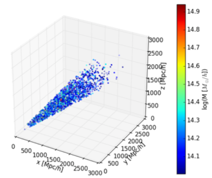
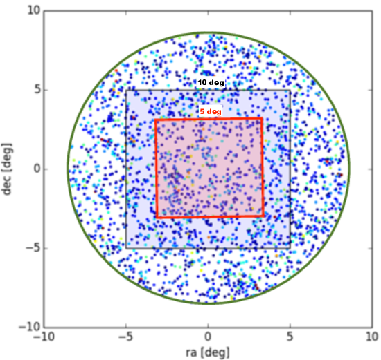
Figure 1: Geometrical construction of the comoving PLC in pinocchio. In the left panel we show the comoving distribution of haloes with mass larger than $10^{14}M_{\odot}/h$ up to redshift $z=4$ present within one realisation. The different masses are colour coded as indicated by the colour bar. In the right panel we display the two-dimensional distribution of those haloes on the plane of the sky in angular coordinates. In this case the choice we have made about the angular geometry of the cone is more visible. The semi-aperture has been set to $7.1$ deg which ensures that a square convergence map with $5$ deg on a side can be simulated. This allows us to take into account the lensing contribution from haloes outside the field-of-view, from a buffer region, and reduce border effects.

2.1 Weak Lensing Maps from N-Body Simulations

In this work we have used the $\mathrm{\Lambda}$CDM run of the CoDECS project (Baldi, 2012) as our reference N-Body simulation. The run has been performed using a modified version of the widely used TreePM/SPH N-body code GADGET (Springel, 2005) developed in Baldi et al. (2010). The CoDECS simulations adopt the following cosmological parameters, consistent with the WMAP7 constraints by Komatsu et al. (2011): $\Omega_{\rm CDM}=0.226$, $\Omega_{b}=0.0451$, $\Omega_{\Lambda}=0.729$, $h=0.703$ and $n_{s}=0.966$, with the initial amplitude of linear scalar perturbations at CMB time ($z_{\rm CMB}\approx 1100$) set to $\mathcal{A}_{s}(z_{\rm CMB})=2.42\times 10^{-9}$, resulting in a value of $\sigma_{8}=0.809$ at $z=0$.

The N-body run follows the evolution $2\times 1024^{3}$ particles evolved through collision-less dynamics from $z=99$ to $z=0$ in a comoving box of $1$ Gpc/$h$ by side. The mass resolution is $m_{\rm CDM}=5.84\times 10^{10}\mathrm{M_{\odot}}/h$ for the cold dark matter component and $m_{b}=1.17\times 10^{10}\mathrm{M_{\odot}}/h$ for baryons, while the gravitational softening was set to $\epsilon_{g}=20\;\mathrm{kpc}/h$. Despite the presence of baryonic particles this simulation does not include hydrodynamics and is therefore a purely collision-less N-body run. This is due to the original purpose of the CoDECS simulations to capture the non-universal coupling of a light dark energy scalar field to Dark Matter particles only, leaving baryons uncoupled. Clearly, for the reference $\mathrm{\Lambda}$CDM run – where the coupling is set to zero – no difference is to be expected in the gravitational evolution of the Dark Matter and baryonic components, which should be considered just as two families of collision-less particles.

To build the lensing maps for light-cone simulations we stacked together different slices of the simulation snapshots up to $z_{s}=4$. We have constructed the PLC to have an angular squared aperture of $5$ deg on a side, which combined with the comoving size of the simulation box of $1$ Gpc/$h$, ensures that the mass density distribution in the cone has no gaps. By construction, the geometry of the PLC is a pyramid with a squared base, where the observer is located at the vertex of the solid figure, while the final source redshift is placed at the base. In stacking up the various simulation snapshots and collapsing them into projected particle lens planes we make use of the MapSim code (Giocoli et al., 2015; Tessore et al., 2015; Castro et al., 2018; Hilbert et al., 2019). The code initialises the memory and the grid size of the maps and reads particle positions within the desired field of view (in this case, $5$ deg on a side) from single snapshot files, which reduces the memory consumption significantly. The algorithm builds up the lens planes from the present time up to the highest source redshift, selected to be $z_{s}=4$. The number of required lens planes is decided ahead of time in order to avoid gaps in the constructed light-cones. The lens planes are built by mapping the particle positions to the nearest predetermined plane, maintaining angular positions, and then pixelizing the surface density using the Triangular Shaped Cloud (TSC) mass assignment scheme (Hockney & Eastwood, 1988). The grid pixels are chosen to have the same angular size on all planes, equal to $2048\times 2048$, which allows for a resolution of $8.8$ arcsec per pixel. The lens planes have been constructed each time a piece of simulation is taken from the stored particle snapshots; their number and recurrence depend on the number of snapshots stored while running the simulation. In particular, in running our simulation we have stored $17$ snapshots from $z\sim 4$ to $z=0$. In Castro et al. (2018) it has been shown that a similar number of snapshots is enough to reconstruct the PLC up to $z\sim 5$ with lensing statistics changing by less than $1\%$ if more snapshots are used.

The selection and the randomisation of each snapshot is done as in Roncarelli et al. (2007) and discussed in more details in Giocoli et al. (2015). If the light-cone arrives at the border of a simulation box before it reaches the redshift limit where the next snapshot will be used, the box is re-randomised and the light-cone extended through it again. Once the lens planes are created the lensing calculation itself is done using the ray-tracing glamer pipeline (Metcalf & Petkova, 2014; Petkova et al., 2014). In order to have various statistical samples, we have created $25$ light-cone realisations. They can be treated as independent since they do not contain the same structures along the line-of-sight, considering the size of the simulation box to be $1$ Gpc/$h$ and the field of view of $5$ deg on a side. However, it is worth mentioning that all the light-cones are constructed from the same N-body run and that they share the same random realisation of the initial conditions of the Universe. Even if their reconstructed lensing signal on small scales depends on matter that occurs in the field-of-view, the large scale modes are established by the seed in the initial conditions set up when running the numerical simulation.

2.2 Approximate Past-Light-Cones using Pinocchio

We will compare the lensing simulations performed using the N-Body run, with the ones constructed from the halo catalogues built up using a fast and approximate algorithm: pinocchio (namely its version 4.1.1).

pinocchio is an approximate, semi-analytic public code, based on excursion-set theory, ellipsoidal collapse and Lagrangian Perturbation Theory (LPT), that is able to predict the formation of dark matter haloes, given a cosmological linear density field generated on a grid, without running a full N-body simulation. It was presented in Monaco et al. (2002), then extended in Monaco et al. (2013) and Munari et al. (2017). The code first generates a density contrast field on a grid, then it Gaussian-smooths the density using several smoothing radii and computes, using ellipsoidal collapse, the collapse time at each grid point (particle), storing the earliest value. Later, it fragments the collapsed medium with an algorithm that mimics the hierarchical formation of structure. Dark matter haloes are displaced to their final position using LPT. The user can choose which perturbation order to adopt: Zel’dovich Approximation, second-order (2LPT) or third-order (3LPT).

Outputs are given both at fixed times and on the light cone (Munari et al., 2017): for each halo, and for a list of periodic replications needed to tile the comoving volume of the light cone, the code computes the time at which the object crosses the light cone, and outputs its properties (mass, position, velocity) at that time.

Using pinocchio we have produced different simulations as summarised in Table 1. We set cosmology and box properties identical to those used for the reference N-body simulation, but with different initial seed numbers so as to have several realisations of the same volume. This allows us to beat down sample variance on the predicted convergence power spectrum. Our reference pinocchio simulation has been run with $1024^{3}$ grid points and in the 3LPT configuration for the particle displacements starting from the initial conditions. This run consists of $512$ different realisations and corresponding past light-cones. We have chosen the semi-aperture of the past light-cone to be $7.1$ deg which gives a total area in the plane of the sky of $158.37$ deg². This value guarantees us the possibility of creating a pyramidal configuration for the convergence maps – consistent with the maps constructed from the N-body simulation – with $5$ deg by side up to a final source redshift $z_{s}=4$. In addition to the reference pinocchio_3LPT we produced a sample of other approximate simulations: $25$ using the same grid resolutions but adopting both 2LPT and ZA displacements, $512$ with a lower resolution grid ($512^{3}$) and 3LPT, and $25$ with a higher resolution grid ($2048^{3}$) and 3LPT displacements. All corresponding mass resolutions are reported in the third column of Table 1. The random numbers of the initial conditions for the various pinocchio simulations have been consistently chosen to be identical, in the sense that the 512 low resolutions runs with $512^{3}$ grid size have the same initial random displacement fields of the $1024^{3}$, and so the $25$ runs performed with the different displacement fields or using a higher resolution grid of $2048^{3}$ that share the initial condition seeds with the first $25$ reference runs. This will allow us a more direct comparison between the different runs and convergence maps starting from the same initial displacement field of the theoretical linear power spectrum.

The typical CPU for a $1024^{3}$ in 1 Gpc/$h$ N-Body simulations from $z=99$ to $z=0$, plus i/o $90$ snapshots and on-the-fly halo finding procedures is approximately $50.000$ CPU hours; plus $1.000$ more hours for light-cone productions and multi-plane ray-tracing, a typical super architecture like the ones available at CINECA. As for the required resources, a pinocchio run with $1024^{3}$ particles demands a CPU time of order of $10$ hours on a supercomputer; the version with Zel’dovich or 2LPT displacements can fit into a single node with 256 Gb of RAM, while the 3LPT version will require more memory; the elapsed time will be of order of 10 min in this case. Higher orders require a few more FFTs, for an overhead of order of $\sim$10% going from Zel’dovich to 3LPT. The light-cone on-the-fly construction requires an even smaller overhead, $\sim$4% for the configuration used in this paper. The scaling was demonstrated in Munari et al. (2017) to be very similar to $N\log_{2}N$, so going from $512^{3}$ to $1024^{3}$, or from this to $2048^{3}$, requires a factor of $\sim 9$ more computing time and a factor of 8 more memory; if the number of used cores increases as the RAM, the wall-clock time will not change much. Painting haloes on the PLC halo catalogues takes not more than $2$ CPU hours per light-cone, scaling with the number density of systems that depends on the minimum mass threshold considered and on maximum source redshift. This means a ratio of CPU times between full N-Body and Fast Approximate methods in producing one convergence map of $5$ deg by side of approximately $3\times 10^{3}$. To these, we have to highlight the fact that each pinocchio light-cone has the advantage of having a different Initial Condition (IC) set up, while this is not the case for past-light-cones extracted from the N-body.

Table 1: Summary of the simulations. The symbol * marks our reference pinocchio run. For the N-Body case it is worth mentioning that all the various light-cones have been generated from the same cosmological simulation, randomising the various snapshots using the MapSim code. By construction the particle mass resolution of our reference pinocchio run is equal to that of the N-Body simulation; all the runs consider a cosmological box of 1 Gpc/$h$ comoving by side.

	field-of-view [$\mathrm{deg^{2}}$] (haloes)	min. halo mass [$\mathrm{M_{\odot}/}h$]	n. real.	field-of-view [$\mathrm{deg^{2}}$] (convergence)
(*) pinocchio3LPC ($1024^{3}$)	158.37	$7.0\times 10^{11}$	512	25
pinocchio2LPC ($1024^{3}$)	158.37	$7.0\times 10^{11}$	25	25
pinocchioZA ($1024^{3}$)	158.37	$7.0\times 10^{11}$	25	25
pinocchio3LPC ($512^{3}$)	158.37	$5.6\times 10^{12}$	512	25
pinocchio3LPC ($2048^{3}$)	158.37	$8.75\times 10^{10}$	25	25
N-Body	100	$7.0\times 10^{10}$ (total part. mass: DM + bar.)	25	25

In the left panel of Fig. 1 we show the comoving halo distribution in the past-light-cones constructed by pinocchio; haloes have different colour according to their mass, as indicated by the colour-bar. In the right panel we display the two-dimensional distribution of haloes, in angular coordinates as they appear in the plane of the sky up to $z=4$. In the right panel we draw also the size of the squared postage-stamp of $5$ deg by side representing the geometry of our final convergence map. The geometry of pinocchio PLC allows us to consider the lensing contribution from haloes outside the field-of-view, from a buffer region, and accounting also for border effects: lensing signal due to haloes which are not in the final field of $5$ deg by side.

In Figure 2 we show the cumulative halo mass function normalised to a one square degree light-cone, from $z=0$ up to redshift $0.5$, $1.4$ and $4$ from bottom to top, respectively. In both cases haloes have been identified using a Friends-of-Friends algorithm. It is worth to underline that in pinocchio the expression for the threshold distance that determines accretion and merging includes free parameters (Munari et al., 2017) as the linking length parameter for the FoF definition in the N-Body simulations. The comparison of the FoF mass functions between pinocchio and N-Body simulation is fair and consistent, indeed in both cases we use the same methodology to find collapsed structures. For comparison the dotted red curves display the FoF mass function as calibrate by Watson et al. (2013). The lower panels display the relative differences of the median counts computed averaging $25$ different simulation light-cones of the N-Body run with respect to the average predictions from the $512$ pinocchio simulations; the shaded area gives the sample variance measured with the quartiles from pinocchio runs, that is large at low $z$ due to the small sampled volume. Only for comparison purpose, in the top panel we show also the expectation from Sheth & Tormen (1999), where they use the virial definition for the halo mass, and from Tinker et al. (2008); Despali et al. (2016) assuming a threshold corresponding to $200$ times the comoving background density, which has been shown to be the closest to the FoF mass functions (Knebe et al., 2011). In the lower panel we notice that there is a very good agreement between the halo counts in the N-Body and pinocchio light-cones down to $5\times 10^{12}M_{\odot}/h$, however the higher the redshift is the more the N-body counts suffer from a small reduction toward small masses due to particle and force resolutions. The error bars on the green data points and the grey shaded regions enclosing the black lines bracket the first and the third quartiles of the distribution at a fixed halo mass.

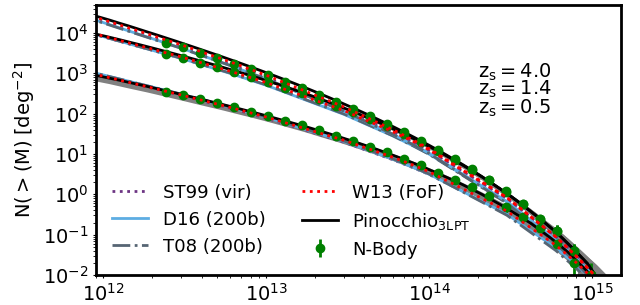
Figure 2: Cumulative halo mass function in unit of square degree within the constructed past-light-cones. The solid black curves display the median over the various realisations, the shaded grey area encloses the quartiles. The green data points indicate the median measurements from the N-Body simulation over $25$ different light-cones. The dotted magenta, solid light-blue, dot-dashed dark grey and red dotted display the predictions from Sheth & Tormen (1999), Despali et al. (2016), Tinker et al. (2008) and Watson et al. (2013) mass functions, respectively. The three bottom sub-panels show the relative difference between the mass function from the N-Body and pinocchio simulations, up to the three considered source redshifts.

2.2.1 Weak lensing simulations using projected halo model

In this section we introduce the lensing notations we will adopt throughout the paper; the symbols and the equations are quite general and consistent between the two methods adopted in constructing the convergence maps from particles and haloes.

Defining ${\boldsymbol{\theta}}$ the angular position on the sky and ${\boldsymbol{\beta}}$ the position on the source plane (the unlensed position), then a distortion matrix ${\bf A}$, in the weak lensing regime, can be read as

$${\bf A}\equiv\frac{\partial{\boldsymbol{\beta}}}{\partial{\boldsymbol{\theta}}}=\left(\begin{array}[]{cc}1-\kappa-\gamma_{1}&\gamma_{2}\\ \gamma_{2}&1-\kappa+\gamma_{1}\end{array}\right)\,,$$ (3)

where scalar $\kappa$ represents the convergence and the pseudo-vector ${\boldsymbol{\gamma}}\equiv\gamma_{1}+i\gamma_{2}$ the shear tensor. In the case of a single lens plane, the convergence can be written as:

$$\kappa({\boldsymbol{\theta}})\equiv\frac{\Sigma({\boldsymbol{\theta}})}{\Sigma_{\rm crit}}\,,$$ (7)

where $\Sigma({\boldsymbol{\theta}})$ represents the surface mass density and $\Sigma_{\rm crit}$ the critical surface density:

$$\Sigma_{\rm crit}\equiv\dfrac{c^{2}}{4\pi G}\dfrac{D_{l}}{D_{s}D_{ls}},$$ (8)

where $c$ indicates the speed of light, $G$ the Newton’s constant and $D_{l}$, $D_{s}$ and $D_{ls}$ the angular diameter distances between observer-lens, observer-source and source-lens, respectively.

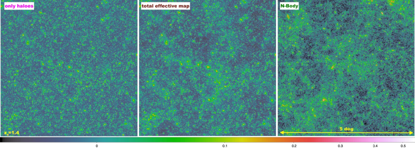
Figure 3: Convergence maps for sources at $z_{s}=1.4$ for a field-of-view of $5\times 5$ square degrees. Left panel shows the map obtained from the halo catalogue of a pinocchio past-light-cone. Central panel displays the effective total contribution of haloes plus not resolved in haloes, modelled using linear theory. Right panel shows, for comparison, the convergence map of a light-cone constructed using MapSim from the snapshots of a cosmological numerical simulation with a different realisation of the initial conditions.

Following a general consensus, we will assume that matter in haloes is distributed following the Navarro et al. (1996) (hereafter NFW) relation:

$$\rho(r|M_{\rm h})=\frac{\rho_{s}}{(r/r_{s})(1+r/r_{s})^{2}}\,,$$ (9)

where $r_{s}$ is the scale radius, defining the concentration $c_{\rm h}\equiv R_{\rm h}/r_{s}$ and $\rho_{s}$ the dark matter density at the scale radius:

$$\rho_{s}=\frac{M_{\rm h}}{4\pi r_{s}^{3}}\left[\ln(1+c_{\rm h})-\frac{c_{\rm h}}{1+c_{\rm h}}\right]^{-1}\,,$$ (10)

$R_{\rm h}$ is the radius of the halo which may vary depending on the halo over-density definition.

From the hierarchical clustering model the halo concentration $c_{\rm h}$ is expected to be a decreasing function of the host halo mass. Small haloes form first (van den Bosch, 2002; De Boni et al., 2016) when the universe was denser and then merge together forming the more massive ones: galaxy clusters sit at the peak of the hierarchical pyramid being the most recent structures to form (Bond et al., 1991; Lacey & Cole, 1993; Sheth & Tormen, 2004a; Giocoli et al., 2007). This trend is reflected in the mass-concentration relation: at a given redshift smaller haloes are more concentrated than larger ones. Different fitting functions for mass-concentration relations have been presented by various authors (Bullock et al., 2001; Neto et al., 2007; Duffy et al., 2008; Gao et al., 2008; Meneghetti et al., 2014; Ragagnin et al., 2019). In this work, we adopt the relation proposed by Zhao et al. (2009) which links the concentration of a given halo with the time $t_{0.04}$ at which its main progenitor assembles $4$ percent of its mass. For the mass accretion history we adopt the model proposed by Giocoli et al. (2012b) which allows us to trace back the full halo growth history with cosmic time down to the desired time $t_{0.04}$. We want to underline that the model by Zhao et al. (2009) also fits numerical simulations with different cosmologies; it seems to be of reasonably general validity within a few percent accuracy, as is the generalised model of the mass accretion history we adopt as tested by Giocoli et al. (2013). It is interesting to notice that the particular model for the concentration mass relation mainly impacts on the behaviour of the power spectrum at scales below $1\,h^{-1}$Mpc as discussed in details by Giocoli et al. (2010). Due to different assembly histories, haloes with the same mass at the same redshift may have different concentrations (Navarro et al., 1996; Jing, 2000; Wechsler et al., 2002; Zhao et al., 2003a, b). At fixed halo mass, the distribution in concentration is well described by a log-normal distribution function with a rms $\sigma_{\ln c}$ between $0.1$ and $0.25$ (Jing, 2000; Dolag et al., 2004; Sheth & Tormen, 2004b; Neto et al., 2007). In this work we adopt a log-normal distribution with $\sigma_{\ln c}=0.25$. We decided to follow this approach in assigning the halo concentration to be as general as possible. Results from the analyses of various numerical simulations have revealed that, at fixed halo mass, structural properties, like concentration and subhalo population, depend on the halo assembly histories (Giocoli et al., 2008, 2010a; Giocoli et al., 2012b; Lange et al., 2019; Zehavi et al., 2019; Montero-Dorta et al., 2020; Chen et al., 2020). However saving all those data three files of the halo catalogues would have increased much the storage capability we planned for this project. As test case in (Giocoli et al., 2017), we have also generated the halo convergence maps reading the halo concentration from the corresponding simulated N-Body catalogue finding that the assembly bias effect on the convergence power spectra has only sub percent effects.
As presented by (Bartelmann, 1996), assuming spherical symmetry the NFW profile has a well defined solution when integrated along the line of sight up to the virial radius:

$$\kappa(x_{1},x_{2}|M_{h},z_{l},z_{s})=2\int_{0}^{R_{\rm vir}}\rho(x_{1},x_{2},\zeta|M_{h})\mathrm{d}\zeta/\Sigma_{crit}(z_{l},z_{s})$$ (11)

with $r^{2}=x_{1}^{2}+x_{2}^{2}+\zeta^{2}$ (Giocoli et al., 2012a; Giocoli et al., 2017). Expressing $\xi^{2}=x_{1}^{2}+x_{2}^{2}$ we can write:

$$\kappa_{0}=2.0/\Sigma_{crit}(z_{l},z_{s}),$$ (12)

and

$$\kappa(\xi)=\kappa_{0}(\kappa_{1}+\kappa_{2}+\kappa_{3})/\kappa_{D},$$ (13)

with

$$\begin{cases}\mathrm{for\;}\xi<1:\\ \kappa_{1}=R_{vir}\sqrt{1-\xi^{2}}\left(1-\sqrt{\xi^{2}+R_{vir}^{2}}\right)\\ \kappa_{2}=-\dfrac{\xi^{2}+R_{vir}^{2}-1}{2}\log\left(\dfrac{\dfrac{R_{vir}}{\sqrt{1-\xi^{2}}}+1}{\dfrac{R_{vir}}{\sqrt{1-\xi^{2}}}-1}\right)\\ \kappa_{3}=\dfrac{\xi^{2}+R_{vir}^{2}-1}{2}\log\left(\dfrac{\left(\dfrac{R_{vir}}{\sqrt{1-\xi^{2}}\sqrt{\xi^{2}+R_{vir}^{2}}}\right)+1}{\left(\dfrac{R_{vir}}{\sqrt{1-\xi^{2}}\sqrt{\xi^{2}+R_{vir}^{2}}}\right)-1}\right)\\ \kappa_{D}=\left(1-\xi^{2}\right)^{3/2}\left(\xi^{2}+R_{vir}^{2}-1\right)\\ \end{cases}$$ (14)

$$\begin{cases}\mathrm{for\;}\xi>1:\\ \kappa_{1}=R_{vir}\sqrt{\xi^{2}-1}\left(\sqrt{\xi^{2}+R_{vir}^{2}}-1\right)\\ \kappa_{2}=-\left(\xi^{2}+R_{vir}^{2}-1\right)\arctan\left(\dfrac{R_{vir}}{\sqrt{\xi^{2}-1}}\right)\\ \kappa_{3}=\left(\xi^{2}+R_{vir}^{2}-1\right)\arctan\left(\dfrac{R_{vir}}{\sqrt{\xi^{2}-1}\sqrt{\xi^{2}+R_{vir}^{2}}}\right)\\ \kappa_{D}=\left(\xi^{2}-1\right)^{3/2}\left(\xi^{2}+R_{vir}^{2}-1\right)\\ \end{cases}$$ (15)

and

$$\begin{cases}\mathrm{for\;}\xi=1:\\ \kappa(\xi)=\dfrac{\kappa_{0}}{3}\sqrt{1+\dfrac{1}{R_{vir}^{2}}}.\end{cases}$$ (16)

The contribution to the convergence from each halo within the field-of-view is modulated by the critical density that depends on the observer-lens-source configuration, as we have expressed in the equations above.

In the left panel of Fig. 3 we show the convergence map reconstructed using halo positions, masses and redshift from one PLC realisation and assuming a fixed source redshift of $z_{s}=1.4$. We can see the contribution from all the mass in the haloes and the presence of galaxy clusters at the intersections of filaments. As discussed by Giocoli et al. (2017) the reconstructed power spectrum using only haloes fails in reproducing the expectation on large scales from linear theory. This inconsistency is a manifestation of the absence of large scale modes sampled by small mass haloes (below our mass resolution threshold) and by the diffuse matter that is not in haloes. A straightforward way to add this power back is to project on the past light-cone particle positions that are outside haloes, construct density planes in redshift bins and add them to those obtained with haloes. This procedure is feasible and will be presented in a future paper; however it implies significant overhead in CPU time and storage: it requires writing particle properties to the disk, something that is avoided by pinocchio in its standard implementation. In the context of the massive generation of mock halo catalogues, it is very convenient to adopt the procedure proposed by Giocoli et al. (2017) to reconstruct the missing power from the halo catalogue itself. We have also estimated the effect of including in the models the missing diffuse matter present between halos by extending the truncation of the density profile at different values of the virial radius. This effect mainly manifests in the transition between the 1- and 2-halo term up to large scales and has not much effect at the 1-halo level, in the projected power spectrum. The extension of the halo density profiles outside the virial radii creates a trend with the source redshifts, artificially increasing the mean background density of the universe, due to the projected intervening matter density distribution along the line-of-sight. Nonetheless, we decided to be conservative in our method, as typically done in the halo model formalism (Cooray & Sheth, 2002), assuming the collapsed matter in haloes only up to the virial radius.

In order to include the large scale modes due to unresolved matter not in haloes, we generate in Fourier space a field with a random Gaussian realisation whose amplitude is modulated by $P_{\kappa,\rm lin}(l)$. The phases are chosen to be coherent with the halo location within the considered map (Giocoli et al., 2017). By construction, summing the convergence maps of the haloes with the one from the linear theory contribution gives a two-dimensional map that includes the cross-talk term between the two fields:

$$\langle\hat{\kappa}(\mathbf{l})\hat{k^{*}}(\mathbf{l}^{\prime})\rangle = \langle\begin{array}[]{c}\mathchoice{\raisebox{-1.07745pt}{\leavevmode\resizebox{444.45099pt}{2.15277pt}{\hbox{\raisebox{506.89pt}{$\displaystyle\mathchoice{\raisebox{0.0pt}{\leavevmode\resizebox{164.31519pt}{505.89pt}{\hbox{\raisebox{0.0pt}{$\displaystyle\mathchoice{\raisebox{0.0pt}{\leavevmode\resizebox{41.0788pt}{505.89pt}{\hbox{\raisebox{2.0pt}{$\displaystyle\kern-0.5pt\bigwedge\kern-0.5pt$}}}}}{\raisebox{0.0pt}{\leavevmode\resizebox{41.0788pt}{505.89pt}{\hbox{\raisebox{2.0pt}{$\textstyle\kern-0.5pt\bigwedge\kern-0.5pt$}}}}}{\raisebox{0.0pt}{\leavevmode\resizebox{41.0788pt}{505.89pt}{\hbox{\raisebox{1.4pt}{$\scriptstyle\kern-0.5pt\bigwedge\kern-0.5pt$}}}}}{\raisebox{0.0pt}{\leavevmode\resizebox{41.0788pt}{505.89pt}{\hbox{\raisebox{1.0pt}{$\scriptscriptstyle\kern-0.5pt\bigwedge\kern-0.5pt$}}}}}$}}}}}{\raisebox{0.0pt}{\leavevmode\resizebox{164.31519pt}{505.89pt}{\hbox{\raisebox{0.0pt}{$\textstyle\mathchoice{\raisebox{0.0pt}{\leavevmode\resizebox{41.0788pt}{505.89pt}{\hbox{\raisebox{2.0pt}{$\displaystyle\kern-0.5pt\bigwedge\kern-0.5pt$}}}}}{\raisebox{0.0pt}{\leavevmode\resizebox{41.0788pt}{505.89pt}{\hbox{\raisebox{2.0pt}{$\textstyle\kern-0.5pt\bigwedge\kern-0.5pt$}}}}}{\raisebox{0.0pt}{\leavevmode\resizebox{41.0788pt}{505.89pt}{\hbox{\raisebox{1.4pt}{$\scriptstyle\kern-0.5pt\bigwedge\kern-0.5pt$}}}}}{\raisebox{0.0pt}{\leavevmode\resizebox{41.0788pt}{505.89pt}{\hbox{\raisebox{1.0pt}{$\scriptscriptstyle\kern-0.5pt\bigwedge\kern-0.5pt$}}}}}$}}}}}{\raisebox{0.0pt}{\leavevmode\resizebox{115.82062pt}{505.89pt}{\hbox{\raisebox{0.0pt}{$\scriptstyle\mathchoice{\raisebox{0.0pt}{\leavevmode\resizebox{28.95515pt}{505.89pt}{\hbox{\raisebox{1.4pt}{$\displaystyle\kern-0.5pt\bigwedge\kern-0.5pt$}}}}}{\raisebox{0.0pt}{\leavevmode\resizebox{28.95515pt}{505.89pt}{\hbox{\raisebox{1.4pt}{$\textstyle\kern-0.5pt\bigwedge\kern-0.5pt$}}}}}{\raisebox{0.0pt}{\leavevmode\resizebox{28.95515pt}{505.89pt}{\hbox{\raisebox{0.98pt}{$\scriptstyle\kern-0.5pt\bigwedge\kern-0.5pt$}}}}}{\raisebox{0.0pt}{\leavevmode\resizebox{28.95515pt}{505.89pt}{\hbox{\raisebox{0.7pt}{$\scriptscriptstyle\kern-0.5pt\bigwedge\kern-0.5pt$}}}}}$}}}}}{\raisebox{0.0pt}{\leavevmode\resizebox{94.15747pt}{505.89pt}{\hbox{\raisebox{0.0pt}{$\scriptscriptstyle\mathchoice{\raisebox{0.0pt}{\leavevmode\resizebox{23.53937pt}{505.89pt}{\hbox{\raisebox{1.0pt}{$\displaystyle\kern-0.5pt\bigwedge\kern-0.5pt$}}}}}{\raisebox{0.0pt}{\leavevmode\resizebox{23.53937pt}{505.89pt}{\hbox{\raisebox{1.0pt}{$\textstyle\kern-0.5pt\bigwedge\kern-0.5pt$}}}}}{\raisebox{0.0pt}{\leavevmode\resizebox{23.53937pt}{505.89pt}{\hbox{\raisebox{0.7pt}{$\scriptstyle\kern-0.5pt\bigwedge\kern-0.5pt$}}}}}{\raisebox{0.0pt}{\leavevmode\resizebox{23.53937pt}{505.89pt}{\hbox{\raisebox{0.5pt}{$\scriptscriptstyle\kern-0.5pt\bigwedge\kern-0.5pt$}}}}}$}}}}}$}}}}}{\raisebox{-1.07745pt}{\leavevmode\resizebox{444.45099pt}{2.15277pt}{\hbox{\raisebox{506.89pt}{$\textstyle\mathchoice{\raisebox{0.0pt}{\leavevmode\resizebox{164.31519pt}{505.89pt}{\hbox{\raisebox{0.0pt}{$\displaystyle\mathchoice{\raisebox{0.0pt}{\leavevmode\resizebox{41.0788pt}{505.89pt}{\hbox{\raisebox{2.0pt}{$\displaystyle\kern-0.5pt\bigwedge\kern-0.5pt$}}}}}{\raisebox{0.0pt}{\leavevmode\resizebox{41.0788pt}{505.89pt}{\hbox{\raisebox{2.0pt}{$\textstyle\kern-0.5pt\bigwedge\kern-0.5pt$}}}}}{\raisebox{0.0pt}{\leavevmode\resizebox{41.0788pt}{505.89pt}{\hbox{\raisebox{1.4pt}{$\scriptstyle\kern-0.5pt\bigwedge\kern-0.5pt$}}}}}{\raisebox{0.0pt}{\leavevmode\resizebox{41.0788pt}{505.89pt}{\hbox{\raisebox{1.0pt}{$\scriptscriptstyle\kern-0.5pt\bigwedge\kern-0.5pt$}}}}}$}}}}}{\raisebox{0.0pt}{\leavevmode\resizebox{164.31519pt}{505.89pt}{\hbox{\raisebox{0.0pt}{$\textstyle\mathchoice{\raisebox{0.0pt}{\leavevmode\resizebox{41.0788pt}{505.89pt}{\hbox{\raisebox{2.0pt}{$\displaystyle\kern-0.5pt\bigwedge\kern-0.5pt$}}}}}{\raisebox{0.0pt}{\leavevmode\resizebox{41.0788pt}{505.89pt}{\hbox{\raisebox{2.0pt}{$\textstyle\kern-0.5pt\bigwedge\kern-0.5pt$}}}}}{\raisebox{0.0pt}{\leavevmode\resizebox{41.0788pt}{505.89pt}{\hbox{\raisebox{1.4pt}{$\scriptstyle\kern-0.5pt\bigwedge\kern-0.5pt$}}}}}{\raisebox{0.0pt}{\leavevmode\resizebox{41.0788pt}{505.89pt}{\hbox{\raisebox{1.0pt}{$\scriptscriptstyle\kern-0.5pt\bigwedge\kern-0.5pt$}}}}}$}}}}}{\raisebox{0.0pt}{\leavevmode\resizebox{115.82062pt}{505.89pt}{\hbox{\raisebox{0.0pt}{$\scriptstyle\mathchoice{\raisebox{0.0pt}{\leavevmode\resizebox{28.95515pt}{505.89pt}{\hbox{\raisebox{1.4pt}{$\displaystyle\kern-0.5pt\bigwedge\kern-0.5pt$}}}}}{\raisebox{0.0pt}{\leavevmode\resizebox{28.95515pt}{505.89pt}{\hbox{\raisebox{1.4pt}{$\textstyle\kern-0.5pt\bigwedge\kern-0.5pt$}}}}}{\raisebox{0.0pt}{\leavevmode\resizebox{28.95515pt}{505.89pt}{\hbox{\raisebox{0.98pt}{$\scriptstyle\kern-0.5pt\bigwedge\kern-0.5pt$}}}}}{\raisebox{0.0pt}{\leavevmode\resizebox{28.95515pt}{505.89pt}{\hbox{\raisebox{0.7pt}{$\scriptscriptstyle\kern-0.5pt\bigwedge\kern-0.5pt$}}}}}$}}}}}{\raisebox{0.0pt}{\leavevmode\resizebox{94.15747pt}{505.89pt}{\hbox{\raisebox{0.0pt}{$\scriptscriptstyle\mathchoice{\raisebox{0.0pt}{\leavevmode\resizebox{23.53937pt}{505.89pt}{\hbox{\raisebox{1.0pt}{$\displaystyle\kern-0.5pt\bigwedge\kern-0.5pt$}}}}}{\raisebox{0.0pt}{\leavevmode\resizebox{23.53937pt}{505.89pt}{\hbox{\raisebox{1.0pt}{$\textstyle\kern-0.5pt\bigwedge\kern-0.5pt$}}}}}{\raisebox{0.0pt}{\leavevmode\resizebox{23.53937pt}{505.89pt}{\hbox{\raisebox{0.7pt}{$\scriptstyle\kern-0.5pt\bigwedge\kern-0.5pt$}}}}}{\raisebox{0.0pt}{\leavevmode\resizebox{23.53937pt}{505.89pt}{\hbox{\raisebox{0.5pt}{$\scriptscriptstyle\kern-0.5pt\bigwedge\kern-0.5pt$}}}}}$}}}}}$}}}}}{\raisebox{0.0pt}{\leavevmode\resizebox{377.0257pt}{2.15277pt}{\hbox{\raisebox{0.0pt}{$\scriptstyle\mathchoice{\raisebox{0.0pt}{\leavevmode\resizebox{115.02063pt}{505.89pt}{\hbox{\raisebox{0.0pt}{$\displaystyle\mathchoice{\raisebox{0.0pt}{\leavevmode\resizebox{28.75516pt}{505.89pt}{\hbox{\raisebox{1.4pt}{$\displaystyle\kern-0.5pt\bigwedge\kern-0.5pt$}}}}}{\raisebox{0.0pt}{\leavevmode\resizebox{28.75516pt}{505.89pt}{\hbox{\raisebox{1.4pt}{$\textstyle\kern-0.5pt\bigwedge\kern-0.5pt$}}}}}{\raisebox{0.0pt}{\leavevmode\resizebox{28.75516pt}{505.89pt}{\hbox{\raisebox{0.98pt}{$\scriptstyle\kern-0.5pt\bigwedge\kern-0.5pt$}}}}}{\raisebox{0.0pt}{\leavevmode\resizebox{28.75516pt}{505.89pt}{\hbox{\raisebox{0.7pt}{$\scriptscriptstyle\kern-0.5pt\bigwedge\kern-0.5pt$}}}}}$}}}}}{\raisebox{0.0pt}{\leavevmode\resizebox{115.02063pt}{505.89pt}{\hbox{\raisebox{0.0pt}{$\textstyle\mathchoice{\raisebox{0.0pt}{\leavevmode\resizebox{28.75516pt}{505.89pt}{\hbox{\raisebox{1.4pt}{$\displaystyle\kern-0.5pt\bigwedge\kern-0.5pt$}}}}}{\raisebox{0.0pt}{\leavevmode\resizebox{28.75516pt}{505.89pt}{\hbox{\raisebox{1.4pt}{$\textstyle\kern-0.5pt\bigwedge\kern-0.5pt$}}}}}{\raisebox{0.0pt}{\leavevmode\resizebox{28.75516pt}{505.89pt}{\hbox{\raisebox{0.98pt}{$\scriptstyle\kern-0.5pt\bigwedge\kern-0.5pt$}}}}}{\raisebox{0.0pt}{\leavevmode\resizebox{28.75516pt}{505.89pt}{\hbox{\raisebox{0.7pt}{$\scriptscriptstyle\kern-0.5pt\bigwedge\kern-0.5pt$}}}}}$}}}}}{\raisebox{0.0pt}{\leavevmode\resizebox{81.07422pt}{505.89pt}{\hbox{\raisebox{0.0pt}{$\scriptstyle\mathchoice{\raisebox{0.0pt}{\leavevmode\resizebox{20.26855pt}{505.89pt}{\hbox{\raisebox{0.98pt}{$\displaystyle\kern-0.5pt\bigwedge\kern-0.5pt$}}}}}{\raisebox{0.0pt}{\leavevmode\resizebox{20.26855pt}{505.89pt}{\hbox{\raisebox{0.98pt}{$\textstyle\kern-0.5pt\bigwedge\kern-0.5pt$}}}}}{\raisebox{0.0pt}{\leavevmode\resizebox{20.26855pt}{505.89pt}{\hbox{\raisebox{0.68599pt}{$\scriptstyle\kern-0.5pt\bigwedge\kern-0.5pt$}}}}}{\raisebox{0.0pt}{\leavevmode\resizebox{20.26855pt}{505.89pt}{\hbox{\raisebox{0.48999pt}{$\scriptscriptstyle\kern-0.5pt\bigwedge\kern-0.5pt$}}}}}$}}}}}{\raisebox{0.0pt}{\leavevmode\resizebox{65.91022pt}{505.89pt}{\hbox{\raisebox{0.0pt}{$\scriptscriptstyle\mathchoice{\raisebox{0.0pt}{\leavevmode\resizebox{16.47755pt}{505.89pt}{\hbox{\raisebox{0.7pt}{$\displaystyle\kern-0.5pt\bigwedge\kern-0.5pt$}}}}}{\raisebox{0.0pt}{\leavevmode\resizebox{16.47755pt}{505.89pt}{\hbox{\raisebox{0.7pt}{$\textstyle\kern-0.5pt\bigwedge\kern-0.5pt$}}}}}{\raisebox{0.0pt}{\leavevmode\resizebox{16.47755pt}{505.89pt}{\hbox{\raisebox{0.48999pt}{$\scriptstyle\kern-0.5pt\bigwedge\kern-0.5pt$}}}}}{\raisebox{0.0pt}{\leavevmode\resizebox{16.47755pt}{505.89pt}{\hbox{\raisebox{0.34999pt}{$\scriptscriptstyle\kern-0.5pt\bigwedge\kern-0.5pt$}}}}}$}}}}}$}}}}}{\raisebox{0.0pt}{\leavevmode\resizebox{269.3034pt}{2.15277pt}{\hbox{\raisebox{0.0pt}{$\scriptscriptstyle\mathchoice{\raisebox{0.0pt}{\leavevmode\resizebox{82.15735pt}{505.89pt}{\hbox{\raisebox{0.0pt}{$\displaystyle\mathchoice{\raisebox{0.0pt}{\leavevmode\resizebox{20.53934pt}{505.89pt}{\hbox{\raisebox{1.0pt}{$\displaystyle\kern-0.5pt\bigwedge\kern-0.5pt$}}}}}{\raisebox{0.0pt}{\leavevmode\resizebox{20.53934pt}{505.89pt}{\hbox{\raisebox{1.0pt}{$\textstyle\kern-0.5pt\bigwedge\kern-0.5pt$}}}}}{\raisebox{0.0pt}{\leavevmode\resizebox{20.53934pt}{505.89pt}{\hbox{\raisebox{0.7pt}{$\scriptstyle\kern-0.5pt\bigwedge\kern-0.5pt$}}}}}{\raisebox{0.0pt}{\leavevmode\resizebox{20.53934pt}{505.89pt}{\hbox{\raisebox{0.5pt}{$\scriptscriptstyle\kern-0.5pt\bigwedge\kern-0.5pt$}}}}}$}}}}}{\raisebox{0.0pt}{\leavevmode\resizebox{82.15735pt}{505.89pt}{\hbox{\raisebox{0.0pt}{$\textstyle\mathchoice{\raisebox{0.0pt}{\leavevmode\resizebox{20.53934pt}{505.89pt}{\hbox{\raisebox{1.0pt}{$\displaystyle\kern-0.5pt\bigwedge\kern-0.5pt$}}}}}{\raisebox{0.0pt}{\leavevmode\resizebox{20.53934pt}{505.89pt}{\hbox{\raisebox{1.0pt}{$\textstyle\kern-0.5pt\bigwedge\kern-0.5pt$}}}}}{\raisebox{0.0pt}{\leavevmode\resizebox{20.53934pt}{505.89pt}{\hbox{\raisebox{0.7pt}{$\scriptstyle\kern-0.5pt\bigwedge\kern-0.5pt$}}}}}{\raisebox{0.0pt}{\leavevmode\resizebox{20.53934pt}{505.89pt}{\hbox{\raisebox{0.5pt}{$\scriptscriptstyle\kern-0.5pt\bigwedge\kern-0.5pt$}}}}}$}}}}}{\raisebox{0.0pt}{\leavevmode\resizebox{57.91022pt}{505.89pt}{\hbox{\raisebox{0.0pt}{$\scriptstyle\mathchoice{\raisebox{0.0pt}{\leavevmode\resizebox{14.47755pt}{505.89pt}{\hbox{\raisebox{0.7pt}{$\displaystyle\kern-0.5pt\bigwedge\kern-0.5pt$}}}}}{\raisebox{0.0pt}{\leavevmode\resizebox{14.47755pt}{505.89pt}{\hbox{\raisebox{0.7pt}{$\textstyle\kern-0.5pt\bigwedge\kern-0.5pt$}}}}}{\raisebox{0.0pt}{\leavevmode\resizebox{14.47755pt}{505.89pt}{\hbox{\raisebox{0.48999pt}{$\scriptstyle\kern-0.5pt\bigwedge\kern-0.5pt$}}}}}{\raisebox{0.0pt}{\leavevmode\resizebox{14.47755pt}{505.89pt}{\hbox{\raisebox{0.34999pt}{$\scriptscriptstyle\kern-0.5pt\bigwedge\kern-0.5pt$}}}}}$}}}}}{\raisebox{0.0pt}{\leavevmode\resizebox{47.07849pt}{505.89pt}{\hbox{\raisebox{0.0pt}{$\scriptscriptstyle\mathchoice{\raisebox{0.0pt}{\leavevmode\resizebox{11.76962pt}{505.89pt}{\hbox{\raisebox{0.5pt}{$\displaystyle\kern-0.5pt\bigwedge\kern-0.5pt$}}}}}{\raisebox{0.0pt}{\leavevmode\resizebox{11.76962pt}{505.89pt}{\hbox{\raisebox{0.5pt}{$\textstyle\kern-0.5pt\bigwedge\kern-0.5pt$}}}}}{\raisebox{0.0pt}{\leavevmode\resizebox{11.76962pt}{505.89pt}{\hbox{\raisebox{0.34999pt}{$\scriptstyle\kern-0.5pt\bigwedge\kern-0.5pt$}}}}}{\raisebox{0.0pt}{\leavevmode\resizebox{11.76962pt}{505.89pt}{\hbox{\raisebox{0.25pt}{$\scriptscriptstyle\kern-0.5pt\bigwedge\kern-0.5pt$}}}}}$}}}}}$}}}}}\\ (\kappa_{\rm hm}+\kappa_{\rm lin})\\ \rule{-4.30554pt}{0.0pt}\end{array}(\mathbf{l})\begin{array}[]{c}\mathchoice{\raisebox{-1.07745pt}{\leavevmode\resizebox{474.85101pt}{2.15277pt}{\hbox{\raisebox{506.89pt}{$\displaystyle\mathchoice{\raisebox{0.0pt}{\leavevmode\resizebox{175.5152pt}{505.89pt}{\hbox{\raisebox{0.0pt}{$\displaystyle\mathchoice{\raisebox{0.0pt}{\leavevmode\resizebox{43.8788pt}{505.89pt}{\hbox{\raisebox{2.0pt}{$\displaystyle\kern-0.5pt\bigwedge\kern-0.5pt$}}}}}{\raisebox{0.0pt}{\leavevmode\resizebox{43.8788pt}{505.89pt}{\hbox{\raisebox{2.0pt}{$\textstyle\kern-0.5pt\bigwedge\kern-0.5pt$}}}}}{\raisebox{0.0pt}{\leavevmode\resizebox{43.8788pt}{505.89pt}{\hbox{\raisebox{1.4pt}{$\scriptstyle\kern-0.5pt\bigwedge\kern-0.5pt$}}}}}{\raisebox{0.0pt}{\leavevmode\resizebox{43.8788pt}{505.89pt}{\hbox{\raisebox{1.0pt}{$\scriptscriptstyle\kern-0.5pt\bigwedge\kern-0.5pt$}}}}}$}}}}}{\raisebox{0.0pt}{\leavevmode\resizebox{175.5152pt}{505.89pt}{\hbox{\raisebox{0.0pt}{$\textstyle\mathchoice{\raisebox{0.0pt}{\leavevmode\resizebox{43.8788pt}{505.89pt}{\hbox{\raisebox{2.0pt}{$\displaystyle\kern-0.5pt\bigwedge\kern-0.5pt$}}}}}{\raisebox{0.0pt}{\leavevmode\resizebox{43.8788pt}{505.89pt}{\hbox{\raisebox{2.0pt}{$\textstyle\kern-0.5pt\bigwedge\kern-0.5pt$}}}}}{\raisebox{0.0pt}{\leavevmode\resizebox{43.8788pt}{505.89pt}{\hbox{\raisebox{1.4pt}{$\scriptstyle\kern-0.5pt\bigwedge\kern-0.5pt$}}}}}{\raisebox{0.0pt}{\leavevmode\resizebox{43.8788pt}{505.89pt}{\hbox{\raisebox{1.0pt}{$\scriptscriptstyle\kern-0.5pt\bigwedge\kern-0.5pt$}}}}}$}}}}}{\raisebox{0.0pt}{\leavevmode\resizebox{123.82062pt}{505.89pt}{\hbox{\raisebox{0.0pt}{$\scriptstyle\mathchoice{\raisebox{0.0pt}{\leavevmode\resizebox{30.95515pt}{505.89pt}{\hbox{\raisebox{1.4pt}{$\displaystyle\kern-0.5pt\bigwedge\kern-0.5pt$}}}}}{\raisebox{0.0pt}{\leavevmode\resizebox{30.95515pt}{505.89pt}{\hbox{\raisebox{1.4pt}{$\textstyle\kern-0.5pt\bigwedge\kern-0.5pt$}}}}}{\raisebox{0.0pt}{\leavevmode\resizebox{30.95515pt}{505.89pt}{\hbox{\raisebox{0.98pt}{$\scriptstyle\kern-0.5pt\bigwedge\kern-0.5pt$}}}}}{\raisebox{0.0pt}{\leavevmode\resizebox{30.95515pt}{505.89pt}{\hbox{\raisebox{0.7pt}{$\scriptscriptstyle\kern-0.5pt\bigwedge\kern-0.5pt$}}}}}$}}}}}{\raisebox{0.0pt}{\leavevmode\resizebox{102.15747pt}{505.89pt}{\hbox{\raisebox{0.0pt}{$\scriptscriptstyle\mathchoice{\raisebox{0.0pt}{\leavevmode\resizebox{25.53937pt}{505.89pt}{\hbox{\raisebox{1.0pt}{$\displaystyle\kern-0.5pt\bigwedge\kern-0.5pt$}}}}}{\raisebox{0.0pt}{\leavevmode\resizebox{25.53937pt}{505.89pt}{\hbox{\raisebox{1.0pt}{$\textstyle\kern-0.5pt\bigwedge\kern-0.5pt$}}}}}{\raisebox{0.0pt}{\leavevmode\resizebox{25.53937pt}{505.89pt}{\hbox{\raisebox{0.7pt}{$\scriptstyle\kern-0.5pt\bigwedge\kern-0.5pt$}}}}}{\raisebox{0.0pt}{\leavevmode\resizebox{25.53937pt}{505.89pt}{\hbox{\raisebox{0.5pt}{$\scriptscriptstyle\kern-0.5pt\bigwedge\kern-0.5pt$}}}}}$}}}}}$}}}}}{\raisebox{-1.07745pt}{\leavevmode\resizebox{474.85101pt}{2.15277pt}{\hbox{\raisebox{506.89pt}{$\textstyle\mathchoice{\raisebox{0.0pt}{\leavevmode\resizebox{175.5152pt}{505.89pt}{\hbox{\raisebox{0.0pt}{$\displaystyle\mathchoice{\raisebox{0.0pt}{\leavevmode\resizebox{43.8788pt}{505.89pt}{\hbox{\raisebox{2.0pt}{$\displaystyle\kern-0.5pt\bigwedge\kern-0.5pt$}}}}}{\raisebox{0.0pt}{\leavevmode\resizebox{43.8788pt}{505.89pt}{\hbox{\raisebox{2.0pt}{$\textstyle\kern-0.5pt\bigwedge\kern-0.5pt$}}}}}{\raisebox{0.0pt}{\leavevmode\resizebox{43.8788pt}{505.89pt}{\hbox{\raisebox{1.4pt}{$\scriptstyle\kern-0.5pt\bigwedge\kern-0.5pt$}}}}}{\raisebox{0.0pt}{\leavevmode\resizebox{43.8788pt}{505.89pt}{\hbox{\raisebox{1.0pt}{$\scriptscriptstyle\kern-0.5pt\bigwedge\kern-0.5pt$}}}}}$}}}}}{\raisebox{0.0pt}{\leavevmode\resizebox{175.5152pt}{505.89pt}{\hbox{\raisebox{0.0pt}{$\textstyle\mathchoice{\raisebox{0.0pt}{\leavevmode\resizebox{43.8788pt}{505.89pt}{\hbox{\raisebox{2.0pt}{$\displaystyle\kern-0.5pt\bigwedge\kern-0.5pt$}}}}}{\raisebox{0.0pt}{\leavevmode\resizebox{43.8788pt}{505.89pt}{\hbox{\raisebox{2.0pt}{$\textstyle\kern-0.5pt\bigwedge\kern-0.5pt$}}}}}{\raisebox{0.0pt}{\leavevmode\resizebox{43.8788pt}{505.89pt}{\hbox{\raisebox{1.4pt}{$\scriptstyle\kern-0.5pt\bigwedge\kern-0.5pt$}}}}}{\raisebox{0.0pt}{\leavevmode\resizebox{43.8788pt}{505.89pt}{\hbox{\raisebox{1.0pt}{$\scriptscriptstyle\kern-0.5pt\bigwedge\kern-0.5pt$}}}}}$}}}}}{\raisebox{0.0pt}{\leavevmode\resizebox{123.82062pt}{505.89pt}{\hbox{\raisebox{0.0pt}{$\scriptstyle\mathchoice{\raisebox{0.0pt}{\leavevmode\resizebox{30.95515pt}{505.89pt}{\hbox{\raisebox{1.4pt}{$\displaystyle\kern-0.5pt\bigwedge\kern-0.5pt$}}}}}{\raisebox{0.0pt}{\leavevmode\resizebox{30.95515pt}{505.89pt}{\hbox{\raisebox{1.4pt}{$\textstyle\kern-0.5pt\bigwedge\kern-0.5pt$}}}}}{\raisebox{0.0pt}{\leavevmode\resizebox{30.95515pt}{505.89pt}{\hbox{\raisebox{0.98pt}{$\scriptstyle\kern-0.5pt\bigwedge\kern-0.5pt$}}}}}{\raisebox{0.0pt}{\leavevmode\resizebox{30.95515pt}{505.89pt}{\hbox{\raisebox{0.7pt}{$\scriptscriptstyle\kern-0.5pt\bigwedge\kern-0.5pt$}}}}}$}}}}}{\raisebox{0.0pt}{\leavevmode\resizebox{102.15747pt}{505.89pt}{\hbox{\raisebox{0.0pt}{$\scriptscriptstyle\mathchoice{\raisebox{0.0pt}{\leavevmode\resizebox{25.53937pt}{505.89pt}{\hbox{\raisebox{1.0pt}{$\displaystyle\kern-0.5pt\bigwedge\kern-0.5pt$}}}}}{\raisebox{0.0pt}{\leavevmode\resizebox{25.53937pt}{505.89pt}{\hbox{\raisebox{1.0pt}{$\textstyle\kern-0.5pt\bigwedge\kern-0.5pt$}}}}}{\raisebox{0.0pt}{\leavevmode\resizebox{25.53937pt}{505.89pt}{\hbox{\raisebox{0.7pt}{$\scriptstyle\kern-0.5pt\bigwedge\kern-0.5pt$}}}}}{\raisebox{0.0pt}{\leavevmode\resizebox{25.53937pt}{505.89pt}{\hbox{\raisebox{0.5pt}{$\scriptscriptstyle\kern-0.5pt\bigwedge\kern-0.5pt$}}}}}$}}}}}$}}}}}{\raisebox{0.0pt}{\leavevmode\resizebox{403.90555pt}{2.15277pt}{\hbox{\raisebox{0.0pt}{$\scriptstyle\mathchoice{\raisebox{0.0pt}{\leavevmode\resizebox{122.86058pt}{505.89pt}{\hbox{\raisebox{0.0pt}{$\displaystyle\mathchoice{\raisebox{0.0pt}{\leavevmode\resizebox{30.71515pt}{505.89pt}{\hbox{\raisebox{1.4pt}{$\displaystyle\kern-0.5pt\bigwedge\kern-0.5pt$}}}}}{\raisebox{0.0pt}{\leavevmode\resizebox{30.71515pt}{505.89pt}{\hbox{\raisebox{1.4pt}{$\textstyle\kern-0.5pt\bigwedge\kern-0.5pt$}}}}}{\raisebox{0.0pt}{\leavevmode\resizebox{30.71515pt}{505.89pt}{\hbox{\raisebox{0.98pt}{$\scriptstyle\kern-0.5pt\bigwedge\kern-0.5pt$}}}}}{\raisebox{0.0pt}{\leavevmode\resizebox{30.71515pt}{505.89pt}{\hbox{\raisebox{0.7pt}{$\scriptscriptstyle\kern-0.5pt\bigwedge\kern-0.5pt$}}}}}$}}}}}{\raisebox{0.0pt}{\leavevmode\resizebox{122.86058pt}{505.89pt}{\hbox{\raisebox{0.0pt}{$\textstyle\mathchoice{\raisebox{0.0pt}{\leavevmode\resizebox{30.71515pt}{505.89pt}{\hbox{\raisebox{1.4pt}{$\displaystyle\kern-0.5pt\bigwedge\kern-0.5pt$}}}}}{\raisebox{0.0pt}{\leavevmode\resizebox{30.71515pt}{505.89pt}{\hbox{\raisebox{1.4pt}{$\textstyle\kern-0.5pt\bigwedge\kern-0.5pt$}}}}}{\raisebox{0.0pt}{\leavevmode\resizebox{30.71515pt}{505.89pt}{\hbox{\raisebox{0.98pt}{$\scriptstyle\kern-0.5pt\bigwedge\kern-0.5pt$}}}}}{\raisebox{0.0pt}{\leavevmode\resizebox{30.71515pt}{505.89pt}{\hbox{\raisebox{0.7pt}{$\scriptscriptstyle\kern-0.5pt\bigwedge\kern-0.5pt$}}}}}$}}}}}{\raisebox{0.0pt}{\leavevmode\resizebox{86.6742pt}{505.89pt}{\hbox{\raisebox{0.0pt}{$\scriptstyle\mathchoice{\raisebox{0.0pt}{\leavevmode\resizebox{21.66855pt}{505.89pt}{\hbox{\raisebox{0.98pt}{$\displaystyle\kern-0.5pt\bigwedge\kern-0.5pt$}}}}}{\raisebox{0.0pt}{\leavevmode\resizebox{21.66855pt}{505.89pt}{\hbox{\raisebox{0.98pt}{$\textstyle\kern-0.5pt\bigwedge\kern-0.5pt$}}}}}{\raisebox{0.0pt}{\leavevmode\resizebox{21.66855pt}{505.89pt}{\hbox{\raisebox{0.68599pt}{$\scriptstyle\kern-0.5pt\bigwedge\kern-0.5pt$}}}}}{\raisebox{0.0pt}{\leavevmode\resizebox{21.66855pt}{505.89pt}{\hbox{\raisebox{0.48999pt}{$\scriptscriptstyle\kern-0.5pt\bigwedge\kern-0.5pt$}}}}}$}}}}}{\raisebox{0.0pt}{\leavevmode\resizebox{71.5102pt}{505.89pt}{\hbox{\raisebox{0.0pt}{$\scriptscriptstyle\mathchoice{\raisebox{0.0pt}{\leavevmode\resizebox{17.87755pt}{505.89pt}{\hbox{\raisebox{0.7pt}{$\displaystyle\kern-0.5pt\bigwedge\kern-0.5pt$}}}}}{\raisebox{0.0pt}{\leavevmode\resizebox{17.87755pt}{505.89pt}{\hbox{\raisebox{0.7pt}{$\textstyle\kern-0.5pt\bigwedge\kern-0.5pt$}}}}}{\raisebox{0.0pt}{\leavevmode\resizebox{17.87755pt}{505.89pt}{\hbox{\raisebox{0.48999pt}{$\scriptstyle\kern-0.5pt\bigwedge\kern-0.5pt$}}}}}{\raisebox{0.0pt}{\leavevmode\resizebox{17.87755pt}{505.89pt}{\hbox{\raisebox{0.34999pt}{$\scriptscriptstyle\kern-0.5pt\bigwedge\kern-0.5pt$}}}}}$}}}}}$}}}}}{\raisebox{0.0pt}{\leavevmode\resizebox{288.50333pt}{2.15277pt}{\hbox{\raisebox{0.0pt}{$\scriptscriptstyle\mathchoice{\raisebox{0.0pt}{\leavevmode\resizebox{87.75731pt}{505.89pt}{\hbox{\raisebox{0.0pt}{$\displaystyle\mathchoice{\raisebox{0.0pt}{\leavevmode\resizebox{21.93933pt}{505.89pt}{\hbox{\raisebox{1.0pt}{$\displaystyle\kern-0.5pt\bigwedge\kern-0.5pt$}}}}}{\raisebox{0.0pt}{\leavevmode\resizebox{21.93933pt}{505.89pt}{\hbox{\raisebox{1.0pt}{$\textstyle\kern-0.5pt\bigwedge\kern-0.5pt$}}}}}{\raisebox{0.0pt}{\leavevmode\resizebox{21.93933pt}{505.89pt}{\hbox{\raisebox{0.7pt}{$\scriptstyle\kern-0.5pt\bigwedge\kern-0.5pt$}}}}}{\raisebox{0.0pt}{\leavevmode\resizebox{21.93933pt}{505.89pt}{\hbox{\raisebox{0.5pt}{$\scriptscriptstyle\kern-0.5pt\bigwedge\kern-0.5pt$}}}}}$}}}}}{\raisebox{0.0pt}{\leavevmode\resizebox{87.75731pt}{505.89pt}{\hbox{\raisebox{0.0pt}{$\textstyle\mathchoice{\raisebox{0.0pt}{\leavevmode\resizebox{21.93933pt}{505.89pt}{\hbox{\raisebox{1.0pt}{$\displaystyle\kern-0.5pt\bigwedge\kern-0.5pt$}}}}}{\raisebox{0.0pt}{\leavevmode\resizebox{21.93933pt}{505.89pt}{\hbox{\raisebox{1.0pt}{$\textstyle\kern-0.5pt\bigwedge\kern-0.5pt$}}}}}{\raisebox{0.0pt}{\leavevmode\resizebox{21.93933pt}{505.89pt}{\hbox{\raisebox{0.7pt}{$\scriptstyle\kern-0.5pt\bigwedge\kern-0.5pt$}}}}}{\raisebox{0.0pt}{\leavevmode\resizebox{21.93933pt}{505.89pt}{\hbox{\raisebox{0.5pt}{$\scriptscriptstyle\kern-0.5pt\bigwedge\kern-0.5pt$}}}}}$}}}}}{\raisebox{0.0pt}{\leavevmode\resizebox{61.91022pt}{505.89pt}{\hbox{\raisebox{0.0pt}{$\scriptstyle\mathchoice{\raisebox{0.0pt}{\leavevmode\resizebox{15.47755pt}{505.89pt}{\hbox{\raisebox{0.7pt}{$\displaystyle\kern-0.5pt\bigwedge\kern-0.5pt$}}}}}{\raisebox{0.0pt}{\leavevmode\resizebox{15.47755pt}{505.89pt}{\hbox{\raisebox{0.7pt}{$\textstyle\kern-0.5pt\bigwedge\kern-0.5pt$}}}}}{\raisebox{0.0pt}{\leavevmode\resizebox{15.47755pt}{505.89pt}{\hbox{\raisebox{0.48999pt}{$\scriptstyle\kern-0.5pt\bigwedge\kern-0.5pt$}}}}}{\raisebox{0.0pt}{\leavevmode\resizebox{15.47755pt}{505.89pt}{\hbox{\raisebox{0.34999pt}{$\scriptscriptstyle\kern-0.5pt\bigwedge\kern-0.5pt$}}}}}$}}}}}{\raisebox{0.0pt}{\leavevmode\resizebox{51.07849pt}{505.89pt}{\hbox{\raisebox{0.0pt}{$\scriptscriptstyle\mathchoice{\raisebox{0.0pt}{\leavevmode\resizebox{12.76962pt}{505.89pt}{\hbox{\raisebox{0.5pt}{$\displaystyle\kern-0.5pt\bigwedge\kern-0.5pt$}}}}}{\raisebox{0.0pt}{\leavevmode\resizebox{12.76962pt}{505.89pt}{\hbox{\raisebox{0.5pt}{$\textstyle\kern-0.5pt\bigwedge\kern-0.5pt$}}}}}{\raisebox{0.0pt}{\leavevmode\resizebox{12.76962pt}{505.89pt}{\hbox{\raisebox{0.34999pt}{$\scriptstyle\kern-0.5pt\bigwedge\kern-0.5pt$}}}}}{\raisebox{0.0pt}{\leavevmode\resizebox{12.76962pt}{505.89pt}{\hbox{\raisebox{0.25pt}{$\scriptscriptstyle\kern-0.5pt\bigwedge\kern-0.5pt$}}}}}$}}}}}$}}}}}\\ (\kappa_{\rm hm}+\kappa_{\rm lin})^{*}\\ \rule{-4.30554pt}{0.0pt}\end{array}(\mathbf{l})\rangle$$

$$= 4\pi^{2}\delta_{D}(\mathbf{l}-\mathbf{l}^{\prime})\left(P_{\kappa_{\rm hm}}(l)+P_{\kappa_{\rm lin}}(l)+P_{\rm hm-lin}(l)\right),$$

where $P_{\rm hm-lin}(l)$ indicates the cross-spectrum term between the two fields and, by definition, $P_{\kappa_{\rm lin}}(l)=P_{\kappa_{\rm lin,r}}(l)$, where $P_{\kappa_{\rm lin,r}}(l)$ indicates the power spectrum of a map with random phases. Because of the cross-spectrum term, we then re-normalise the map to match the large scale behaviour predicted on large scale by linear theory using the relation:

$$A(l)=\dfrac{P_{\kappa,\rm lin}(l)}{P_{\kappa_{\rm hm}+\kappa_{\rm lin}}(l)},$$ (24)

where $P_{\kappa_{\rm hm}+\kappa_{\rm lin}}(l)=P_{\kappa_{\rm hm}}(l)+P_{\kappa_{\rm lin}}(l)+P_{\rm hm-lin}(l)$. Dividing the contributions to the convergence power spectrum in haloes and diffuse component allows us to discriminate two separate contributions. While the diffuse matter, relevant on large scales and treated using linear theory, represents the Gaussian contribution to the power spectrum, the haloes, important on small scales in the non linear regime, portrays the non-Gaussian stochastic part. Haloes are non-linear regions of the matter density fluctuation field disjoint from the expansion of the universe, their structural properties – concentration, substructures, density profiles etc – shape the small scale modes (Cooray & Sheth, 2002; Smith et al., 2003; Sheth & Jain, 2003; Giocoli et al., 2010).

In the central panel of Fig. 3 we display the convergence map where we include also the modelling of the large scale modes coherent with the halo distribution within the field of view. In order to do so we use as reference the prediction, in the Fourier space, from the linear theory of the convergence power spectrum $P_{\kappa,\rm lin}(l)$ that in the Born Approximation and for source redshift at $z_{s}$ can be read as:

$$P_{\kappa,\rm lin}(l)=\dfrac{9H_{0}^{4}\Omega_{m}^{2}}{4c^{4}}\int_{0}^{w_{s}(z_{s})}\left(\dfrac{D(z,z_{s})}{D(z_{s})a}\right)^{2}P_{\rm\delta,lin}\left(l\dfrac{a}{D(z)},z\right)\,\mathrm{d}w,$$ (25)

where $H_{0}$ and $\Omega_{m}$ represent the present day Hubble constant and matter density parameter, $c$ indicates the speed of light, $w(z)$ and $D(z)$ the radial comoving and angular diameter distances at redshift $z$, $a\equiv 1/(1+z)$, and $P_{\rm\delta,lin}(k,z)$ the linear matter power spectrum at a given comoving mode $k$ re-scaled by the growth factor at redshift $z$. For comparison, the third panel of Fig. 3 displays the convergence map of the past-light-cone constructed from the cosmological numerical simulation up to $z_{s}=1.4$; we recall that the simulation does not trace the same large-scale structure as the pinocchio realisation.

2.3 Halo Model for non-linear power spectrum

The non-linear matter density distribution for $k>1h/$Mpc can be reconstructed using the halo model formalism. This is based on the assumption that all matter in the universe can be associated to collapsed and virialised haloes. In real space the matter-matter correlation can be decomposed into two components:

$$\xi(r)=\xi_{1h}(r)+\xi_{2h}(r)$$ (26)

where $\xi_{1h}(r)$ and $\xi_{2h}(r)$ are term one and two halo components, that account for the matter-matter correlation in the same or in distant haloes, respectively. Following the halo model formalism as described by (Cooray & Sheth, 2002; Giocoli et al., 2010), we can relate real and Fourier, making explicit the redshift dependence, considering that:

$$P(k,z)=4\pi\int\xi(r,z)\frac{\sin(kr)}{kr}r^{2}{\rm d}r\,,$$ (27)

and write the one and two halo term in Fourier space as:

$$P_{1H}(k,z) = \int_{M_{\rm min}}\left(\dfrac{M_{h}}{\bar{\rho}}\right)^{2}n(M_{h},z)$$ (28)

$$\times \int p(c_{h}|M_{h})u^{2}(k|c_{h}(M_{h}))\mathrm{d}c_{h}\,\mathrm{d}M_{h}\,,$$

$$P_{2H}(k,z) = P_{\rm\delta,lin}(k)\Big{[}\int_{M_{\rm min}}\dfrac{M_{h}}{\bar{\rho}}n(M_{h},z)\,b(M_{h},z)$$ (29)

$$\times \int p(c_{h}|M_{h})\,u(k|c_{h},M_{h})\,\mathrm{d}c_{h}\,\mathrm{d}M_{h}\Big{]}^{2}\,$$

where $u(k|c_{h},M_{h})$ represents the Fourier transform of the NFW matter density profile, $b(M_{h},z)$ the halo bias for which we use the model by Sheth & Tormen (1999) and $n(M_{h},z)$ the halo mass function for which we adopt the Despali et al. (2016) model that describes very well the mass function of pinocchio light-cones, as can be noticed in Fig. 2. In the two equations above we have made it explicit that the halo mass function is typically integrated from a given minimum halo mass $M_{\rm min}$ and that we use a stochastic model for the concentration mass relation with a scatter $\sigma_{\ln c}=0.25$, as considered in wl-moka. It is worth mentioning that eq. 29 needs to be normalised by

$$P_{2H,0}(k,z)=\Big{[}\int_{M_{\rm min}}\dfrac{M_{h}}{\bar{\rho}}n(M_{h},z)\,b(M_{h},z)\,\mathrm{d}M_{h}\Big{]}^{2}\,$$ (30)

since it has to match the linear theory on large scales, i.e. for small $k$.

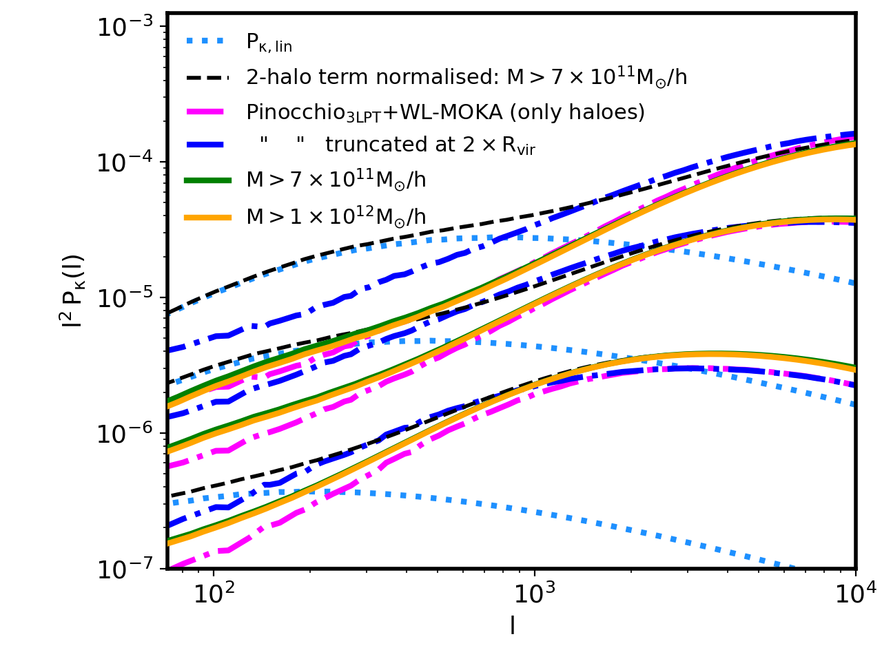
Figure 4: Convergence power spectrum prediction using halo model formalism. The black dashed curves show the prediction at three different fixed source redshifts using eq. (25) (from bottom to top, $z=0.5$, $1.4$ and $4$) where the lower limit of halo mass function integrals is $M_{\rm min}=7\times 10^{11}M_{\odot}/h$ and the two halo term has been normalised using eq. (30) to match the linear prediction – dotted light-blue curves. The magenta (blue) dot-dashed curves show the average measurements done on $512$ convergence maps constructed combining pinocchio PLC and wl-moka using only haloes (truncating the profile at two times the halo virial radius). The green and the orange curves display the analytical halo model prediction summing the contribution of eq. (28) and (29), without normalising the 2-halo term, for two different minimum halo masses.

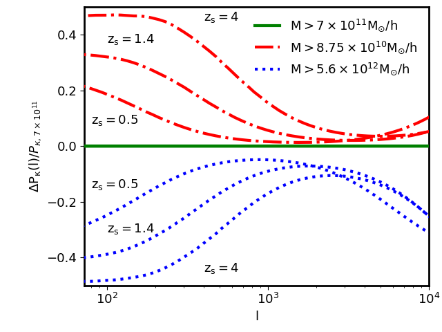
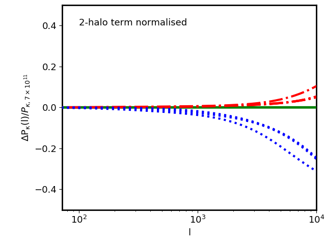
Figure 5: Relative difference of the convergence power spectra, computed using the halo model at three different fixed source redshifts, using different minimum halo mass threshold in the integrals. Left panel shows the relative difference with respect to the prediction of the mass resolution of the reference run of the 1-halo and 2-halo terms summing the contributions from eq. (25) of the expressions in eq. (28) and (29). Right panel displays the relative difference of the total contributions where the 2-halo term has been normalised by eq. (30).

In Fig. 4 we show the halo model predictions for the convergence power spectra, at three different source redshifts (from bottom to top, $z=0.5$, $1.4$ and $4$) integrating the matter power spectra as in eq. (25). The black dashed curves show the prediction of the halo model summing the 1 and 2-halo term, with the latter normalised by the eq. (30) to match on large scales the linear theory power spectra (dotted light-blue lines). The magenta dot-dashed curves exhibit the average convergence power spectra of $512$ maps constructed by wl-moka using haloes from the pinocchio reference runs; for comparison, the blue dot-dashed curves display the results from the $512$ maps created truncating the halo density profiles at two times the virial radius. Green and orange curves display the prediction of the 1 plus 2-halo term not normalised. The fact that the trend of those curves is similar as the pinocchio plus wl-moka indicates that the convergence maps we have constructed using only haloes do not match the predictions from linear theory on large scale. In the analytic halo model formalism this is compensated only in the 2-halo term2, normalising it by an effective bias contribution as in eq. (30), without interfering on the matter density distribution on small scales as described by the 1-halo term. However, it is worth noticing that in the convergence maps constructed using wl-moka we cannot separate a priori the two terms; when including the unresolved matter contribution using linear theory, this will include somehow a small correlation between large and small scales compensating for re-scaling the amplitude as in eq. (24).

In Fig. 5 we display the relative differences, with respect to the case of $M_{min}=7\times 10^{13}M_{\odot}/h$, of the total analytical halo model convergence power spectra, at the same three fixed source redshifts, assuming various minimum halo masses. While on the left panel the 2-halo term is not normalised, in the right panel eq. (29) has been normalised by the effective bias term as in eq. (30). In this latter case we can notice that the mass resolution of the halo model integrals has a negligible effect on large scales, where the 2-halo term is forced to follow linear theory, while on small scales (large $l$) it manifests in appreciable differences.

3 Results

In Fig. 6 we show the convergence power spectra at three source redshifts $z_{s}=4$, $1.4$ and $0.5$ from top to bottom, respectively. The dotted blue curves represent the predictions from linear theory using eq. (25), the dot-dashed magenta ones the average convergence power spectra of the haloes over 512 different realisations of pinocchio light-cones – left panel of Fig. 3. The red (in particular this is a falu red) solid curves display the average power spectra of the 512 simulated convergence fields in which we include also the contribution from unresolved matter (central panel of Fig. 3), the shaded regions enclose the standard deviation of the various realisations. We remind the reader that while the numerical cosmological simulation has been run with only one initial condition displacement field, all $25$ light-cones generated from this have been constructed by randomising the simulation box by translating the particles and redefining the simulation centre when building-up the light-cones. In Fig. 7 we compare the convergence power spectra of our final maps (red solid curves) with the ones from the N-body simulation (green dots). From the figure we notice a very good agreement between our model and the N-body results up to $l\simeq 3\times 10^{3}$ where the green data points start to deviate at low redshifts due to particle shot-noise (Giocoli et al., 2016), and the model tends to move down because of the absence of concentrated low mass haloes below the numerical resolution. The black dashed curves show the corresponding convergence power spectra obtained by integrating the non-linear matter spectra implemented in CAMB by Takahashi et al. (2012). In the bottom sub-panel we display the relative difference between the N-Body predictions and the approximate methods with respect to the non-linear projected matter power spectrum. From the figure we can see that the non-linear predictions are recovered with percent accuracy from $l=72$ (which is the angular mode corresponding to 5 deg) to $l=3\times 10^{3}$ (the largest mode expected to be covered by future wide field surveys) using our approximate methods.

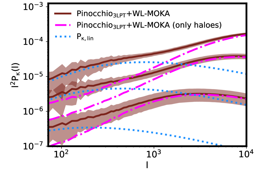
Figure 6: Convergence power spectra at three different source redshifts: from top to bottom $z_{s}=4$, $1.4$ and $0.5$. The dotted blue curves displays the predictions using linear power spectrum, dot-dashed purple the average halo contribution of 512 light-cones from pinocchio. The red lines are the average measurements of 512 realisations of the convergence field from haloes and diffuse component, the shaded regions enclose the rms of the various realisations.

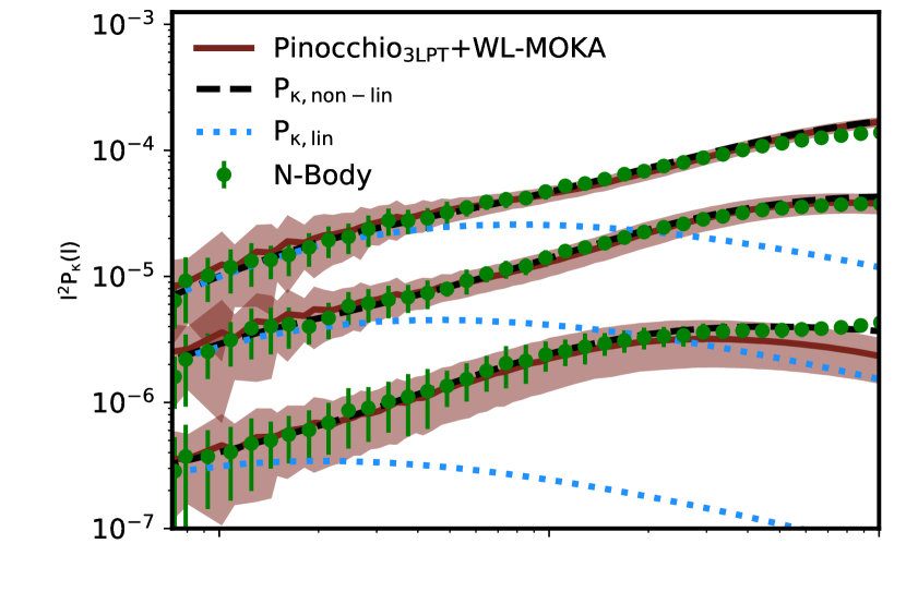
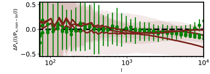
Figure 7: Convergence power spectra at three different source redshifts, from top to bottom $z_{s}=4$, $1.4$ and $0.5$. We compare the predictions using approximate methods pinocchio and WL-MOKA (solid red curves) with measurements from light-cones extracted from a cosmological N-Body simulation using MapSim. Black dashed and blue dotted curves display the predictions using linear and non-linear power spectra from CAMB, the latter refers to the implementation by Takahashi et al. (2012). In the bottom sub-panel we display the relative differences of the N-Body and the approximate convergence power spectra with respect to the non-linear predictions.

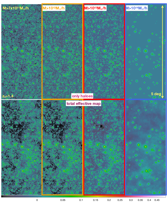
Figure 8: Convergence maps for $z_{s}=4$ constructed adopting different minimum mass thresholds: we use all haloes with mass larger than $7\times 10^{11}$, $10^{12}$, $10^{13}$ and $10^{14}\;M_{\odot}/h$ from left to right, respectively. The top panels show the halo contribution while the bottom ones include also the linear contribution coming from unresolved matter, below the considered minimum halo mass.

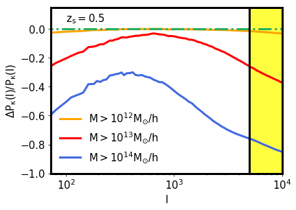
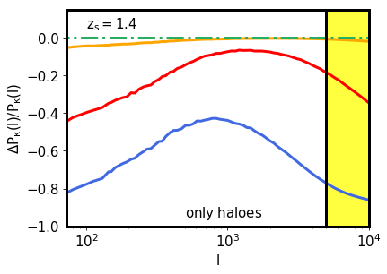
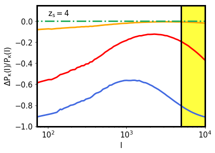
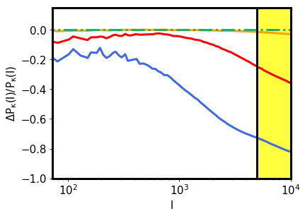
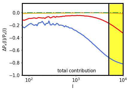
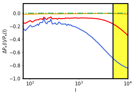
Figure 9: Relative difference in the convergence power spectra adopting various minimum halo mass thresholds at three different source redshifts: $z_{s}=0.5$, $1.4$ and $4$ from left to right, respectively. Orange, red and blue curves display the measurements considering minimum masses of $10^{12}$, $10^{13}$ and $10^{14}\;M_{\odot}/h$ with respect to the reference case that has a minimum halo mass of $7\times 10^{11}\;M_{\odot}/h$. As in Fig. 8, the top panels show the average contribution of $512$ realisations constructed using only haloes while the bottom ones show the average including also the linear contribution coming from unresolved matter, below the considered minimum halo mass. The yellow shaded region marks the region of $l>5\times 10^{3}\;\mathrm{rad}$, up to which future wide field surveys are expected to measure the weak lensing convergence power spectra (Laureijs et al., 2011).

3.1 Stability with minimum halo mass

We profit from the large statistic samples available from the pinocchio runs and we investigate how the reconstruction (Giocoli et al., 2017) of large-scale projected power missing from haloes behaves, as a function of redshift, when a higher threshold for minimum halo mass is used. We run our wl-moka pipeline adopting different threshold for the minimum halo mass. In Fig. 8 we display the convergence map for $z_{s}=1.4$ constructed with a minimum halo mass of $7\times 10^{11}$, $10^{12}$, $10^{13}$ and $10^{14}\;M_{\odot}/h$ from left to right, respectively. The value of $7\times 10^{11}\;M_{\odot}/h$ corresponds to our minimum halo mass in the pinocchio_3LPT reference run, while the case with minimum mass of $10^{14}\;M_{\odot}/h$ will help us in better understanding the contribution of galaxy cluster size-haloes to the weak lensing signal. In the figure, top and bottom panels display the halo and the total contributions to the convergence, respectively. In the latter case we add the linear matter density contribution due to unresolved matter below the corresponding mass threshold limit. From the figure we notice that while clusters represent the high density peaks of the convergence field, smaller mass haloes trace the filamentary structure of the matter density distribution and contribute ,in projection, to increasing the lensing signal (Martinet et al., 2017; Shan et al., 2018; Giocoli et al., 2018).

In Fig. 9 we present the relative difference of the average convergence power spectra, for 512 different realisations, as computed from the different mass threshold maps with respect to the reference one, that has a mass resolution of $7\times 10^{11}\;M_{\odot}/h$. Panels from left to right consider different fixed source redshift $z_{s}=0.5$, $1.4$ and $4$, respectively; while on the top we show only the halo contributions. In the bottom we account also for the contribution from unresolved matter. These figures help us to quantify the contribution of various haloes to the convergence power spectra. In particular, from the top panels we can notice that the contribution of clusters evolves with the redshift going from an average value of approximately $40\%$ for sources at $z_{s}=0.5$ to $10\%$ for $z_{s}=4$. This is an effect where the cluster contribution is modulated by the lensing kernel, depending on the considered source redshift, and it is sensitive to the redshift evolution of the cluster mass function. On the other side, in the bottom panels we can notice that the average power spectra from total effective convergence maps built using only clusters deviates by approximately $30\%$ with respect to the reference ones, independently of the source redshift. The yellow shaded region, in the right part of each panel, indicates where future wide field surveys like the ESA Euclid mission will not be able to provide any reliable data; future wide field missions will be able to probe the convergence power spectrum up to $l\approx 3\times 10^{3}$.

As discussed by Munari et al. (2017) and Paranjape et al. (2013) in pinocchio the bias of dark matter haloes is a prediction. This applies also when the code is interfaced with wl-moka in creating effective convergence maps. In particular the square-root of the ratio at large angular scales (the comoving scale of $k=0.1h$ Mpc^-1 corresponds approximately to $l\approx 150$, $300$ and $520$ for source redshift $z_{s}=0.5$, $1,4$ and $4$, respectively) between the halo and the total convergence power spectrum gives us a measure of the projected halo bias. This can be modelled using the two halo term of the projected halo model as discussed in Sec. 2.3.

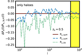
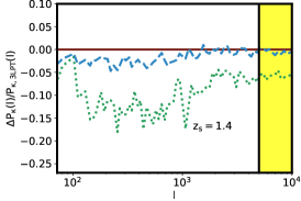
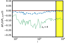
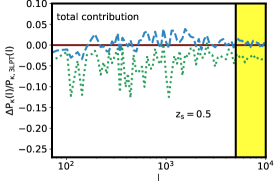
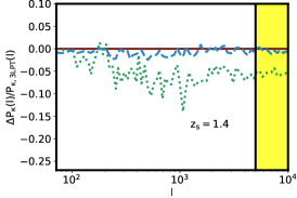
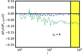
Figure 10: Relative convergence power spectra between maps constructed using pinocchio 2LPT (dashed blue) and ZA (dotted green) with respect to 3LPT. From left to right we show the cases for the three considered source redshifts: $z_{s}=0.5$, $1.4$ and $4$, respectively. Top and bottom panels show the cases in which the maps are constructed using only haloes or haloes plus diffuse matter.

3.2 LPT order for the displacement fields

As presented by Munari et al. (2017), in the new version of pinocchio the user can run the code adopting different LPT orders for particle displacement fields: ZA (Zel’dovich Approximation), 2LPT and 3LPT. In this section we investigate how the reconstructed convergence power spectra, at different fixed source redshifts, depends on the adopted displacement order. In Fig. 10 we show the relative difference of the convergence power spectra at three source redshifts. Blue dashed and green dotted curves display the relative difference of the ZA and 2LPT cases with respect to the 3LPT. While the top panels exhibit the power spectra due only to resolved haloes in the light-cone simulations, the bottom ones account also for the corresponding contribution due to matter among haloes. In the bottom panels, where we have the total contribution, while the 2LPT case differs from the 3LPT case by less than $1\%$, the ZA case tends to deviate more than $5-7\%$ with larger deviations for larger angular modes (small scales) reaching values of $\sim 10\%$. We remind the reader that the average measurements are done only on $25$ different light-cone runs and the simulations, with various displacement prescription, share the same seeds and phases, when generating the initial conditions.

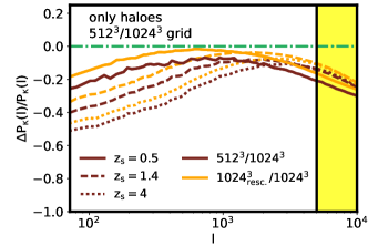
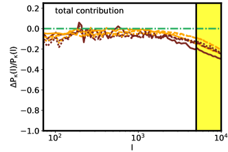
Figure 11: Relative difference between the $512^{3}$ and the $1024^{3}$ simulations. The different curves show the results for the three source redshifts, left and right panels refer to the case where we consider the contribution only from haloes or we include also the diffuse matter using linear theory, respectively. The orange curves display the relative difference when building the maps from the $1024^{3}$ we adopt the same minimum halo mass resolution of the $512^{3}$, namely $5.6\times 10^{12}M_{\odot}/h$.

3.3 Resolution of Approximate Method Simulations

The reconstructed 2D field using the halo model technique depends also on the resolution of the grid mesh on the top of which the halo catalogue is constructed in the PLC. As for numerical simulations that solve the full N-Body relations, pinocchio runs are much faster when the displacement grid is coarser. In Fig. 11 we show the case in which we compare the convergence power spectra of $512$ approximate methods past-light-cones with grid resolution of $512^{3}$ and our reference run of $1024^{3}$; in both cases we assume a 3LPT displacement field and the same initial seeds for the initial conditions. The orange curves display the relative difference of the $1024^{3}$ maps re-scaled to the same resolution of the $512^{3}$ with respect to the reference resolution run. Left and right panel show the comparison of the power spectra coming only from the haloes and from the full projected matter density distribution (haloes plus unresolved matter treated using linear theory). From the left figure we can see that the runs with lower resolution have a redshift dependence trend at low angular modes (larger scales). These are integrated effects due to the haloes that mainly contribute to the lensing signal when accounting for the lensing kernel at a given source redshift. However, from the right figure we can notice that when adding the contribution coming from unresolved matter using linear theory (right panel) this redshift tendency disappears, and on average up to $l=3\times 10^{3}$ the relative difference of the low resolution run is between 5 and $10\%$. At those scales it is evident that the simulations constructed from the coarser grid are missing concentrated small haloes. In re-scaling the $1024^{3}$ to the same map resolution of the $512^{3}$, namely $5.6\times 10^{12}\,M_{\odot}/h$, we notice few percent deviations probably attributed to the different displacement grids of the two runs, halo finding threshold resolution when linking particles in friends of friends and halo bias that enter on the two halo term on large scale, even if the two PLC have the same minimum halo mass.

Fig. 12 displays the relative difference between full power spectra of $25$ high resolution and reference runs that share the same initial condition seeds. As in the previous figures, the different line types refer to various fixed source redshifts. As we can read from Table 1 the run with $2048^{3}$ grid mesh has a minimum halo mass a factor of 8 lower than the one with $1024^{3}$. The figure shows that convergence power spectra computed from the high resolution runs are approximately $3-5\%$ higher that the ones from our reference simulations. This difference probably arises from the fact that when including the contribution from diffuse matter in our convergence halo maps we are not able to specifically separate the 1 and 2-halo term – as we do analytically in the halo model as discussed in section 2.3, causing a small shift up. However, we want to underline that the main goal of our approach is to be able to build a fast and self-consistent method for covariances; many faster and more accurate approaches already exist in term of non-linear power spectra that will be used for modelling the small scales observed signals from future weak lensing surveys (Peacock & Dodds, 1996; Smith et al., 2003; Takahashi et al., 2012; Debackere et al., 2019; Schneider et al., 2019).

For summary, we address the reader to Appendix B where we show the convergence maps build using different particle and grid resolutions, while adopting the same initial displacement seed and phases. The maps refer to light-cones build only from haloes up to $z_{s}=1.4$.

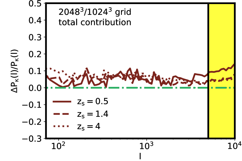
Figure 12: Relative difference between the convergence power spectra in the $2048^{3}$ and $1024^{3}$ runs. The relative difference has been computed as average of $25$ difference past-light-cone realisations considering both haloes and diffuse matter.

In Fig. 13 we show the relative difference of the average power spectra computed from $512$ different past light-cones with $1024^{3}$ grid mesh with respect to the prediction obtained integrating the non-linear matter power spectrum from CAMB using the Takahashi et al. (2012) implementation. The dark grey, grey and light grey regions mark the relative difference of $5$, $15$ and $25\%$, blue data points with the corresponding error bars are the convergence power spectra prediction obtained by Izard et al. (2018) using ICE-COLA with respect to the MICE simulation for sources at $z_{s}=1$. These comparisons strengthen the power of the two methods pinocchio plus wl-moka in reconstructing the projected non-linear power spectrum, and the flexibility to use different fixed source redshifts or a defined source redshift distribution of sources. The limit of these runs are related to the small field of view we have decided to simulate, but this will be extended in a future dedicated work as well as the possibility to construct convergence on HEALPix maps.

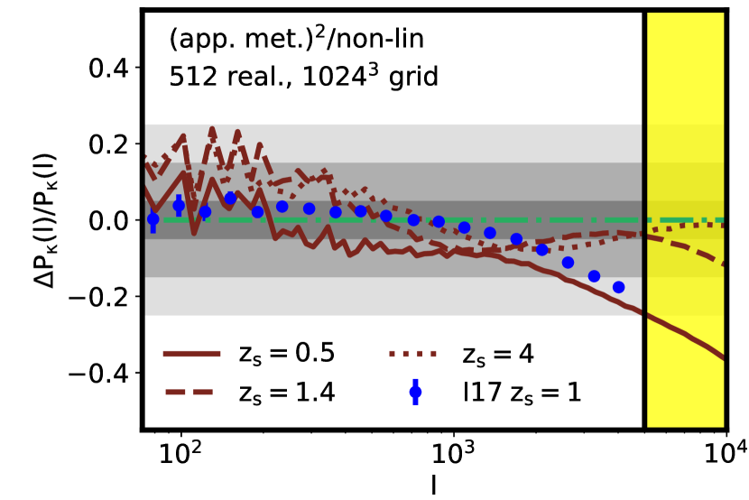
Figure 13: Relative difference between convergence power spectra computed using approximate methods and the prediction from non-linear matter power spectrum as implemented in CAMB by Takahashi et al. (2012). The different curves red curves show the results for the three considered source redshifts, while the data points displays the results obtained by Izard et al. (2018) for $z_{s}=1$ comparing their approximate methods for weak lensing, based on ICE-COLA, with respect to the reference MICE simulation. In the figure the red curves show the average values obtained on $512$ pinocchio light-cone realisations with a grid resolution of $1024^{3}$. Dark-grey, grey and light-grey bands indicate $5$, $15$ and $25\%$ relative differences.

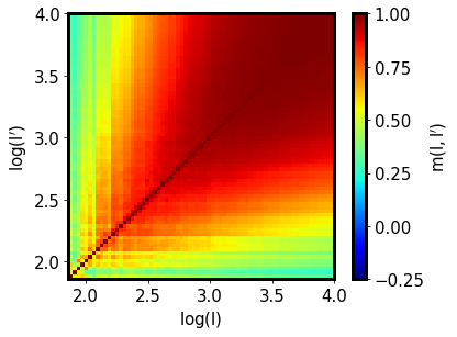
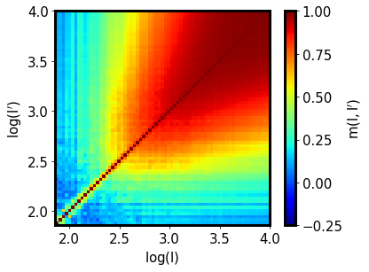
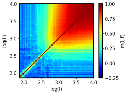
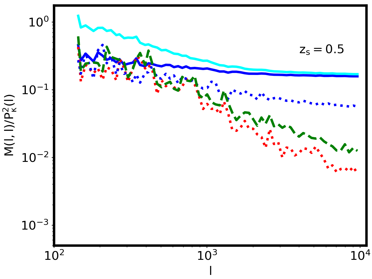
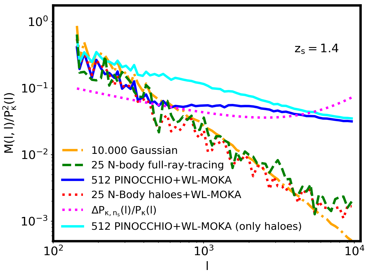
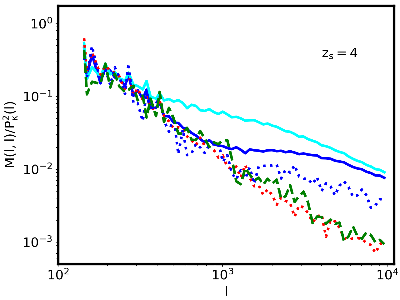
Figure 14: Top panels: weak lensing covariance matrices for $z_{s}=0.5$, $1.4$ and $4$ from left to right, respectively, constructed from 512 past-light-cone pinocchio simulations – 3LPT runs with a grid of $1024^{3}$ – and using our fast weak lensing halo model wl-moka. The aperture of the field of view is set to 5 deg on a side and convergence maps are resolved with $2048^{2}$ pixels. Bottom panels: signal-to-noise of the diagonal term of different covariance matrices. In the central panel (the closest to the mean of the source redshift distribution useful from weak lensing expected from future wide-field-survey) we display also the result from Gaussian covariance (dash-dotted orange curve) and from the observational discrete number density of background sources (Refregier et al., 2004) adopting a Euclid-like sky coverage of 15.000 sq. degs. and 30 galaxies per square arcmin (dotted magenta).

The inference for cosmological parameters, expressed in term of the data vector $\vec{\Theta}$, using weak gravitational lensing is found by minimising the likelihood function that compares observational data to reference models (Takada & Jain, 2004; Simon et al., 2004; Kilbinger et al., 2013; Kitching et al., 2014; Köhlinger et al., 2017). In the case of Gaussian distributed data the likelihood can be approximated as:

$$\mathcal{\ln L}(\vec{\Theta})\propto-\dfrac{1}{2}\sum_{i,j=1}^{N_{b}}\left[P^{``obs^{\prime\prime}}_{\kappa}(l_{i})-P_{\kappa}(l_{i},\vec{\Theta})\right]M(l_{i},l_{j})^{-1}$$

$$\left[P^{``obs^{\prime\prime}}_{\kappa}(l_{j})-P_{\kappa}(l_{j},\vec{\Theta})\right]\,,$$ (31)

where $M(l,l^{\prime})$ represents the covariance matrix; its inverse is usually termed precision matrix. It is worth noting that in the equation above we have neglected the cosmological dependence of the covariance matrix. However, this is the subject of ongoing study and discussion (Labatie et al., 2012; Harnois-Déraps et al., 2019) and we plan to address it in a future work focused both on clustering and weak gravitational lensing.

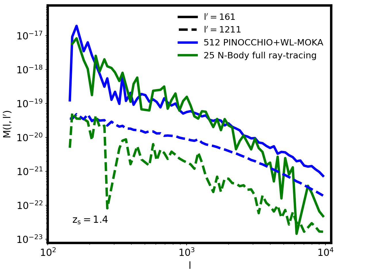
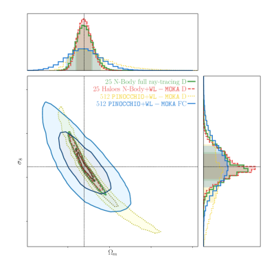
Figure 15: Left panel: comparison between off-diagonal covariance matrix terms, at two fixed values for $l^{\prime}$, computed from $25$ N-Body full ray-tracing simulations and $512$ simulations obtained using the approximate methods for $z_{s}=1.4$. Right panel: 1 and 2 $\sigma$ cosmological constraints in the $\Omega_{m}$-$\sigma_{8}$ parameter space computed adopting different covariances for $z_{s}=1.4$. Green and red contours adopt the diagonal term of the covariances constructed from $25$ N-Body convergence map realisations using particle full ray-tracing and halo population plus WL-MOKA as in Giocoli et al. (2017), respectively. The yellow and blue contours make use of the covariance from $512$ approximate methods convergence maps: considering only the diagonal (D) or the full covariance (FC), respectively. Being interested in the relative performances of the various covariance terms, we follow the same approach as in Krause & Eifler (2017) not including the axis values.

Using different weak lensing light-cone realisations we can build the covariance matrix as:

$$M(l,l^{\prime})=\langle(P_{\kappa}(l)-\bar{P}_{\kappa}(l))(P_{\kappa}(l^{\prime})-\bar{P}_{\kappa}(l^{\prime}))\rangle$$ (32)

where $\langle\bar{P}_{\kappa}(l)\rangle$ represents the best estimate of the power spectrum at the mode $l$ obtained from the average, or the median, of all the corresponding light-cone realisations and $P_{\kappa}(l)$ represents the measurement of one realisation. The matrix is then normalised as follows:

$$m(l,l^{\prime})=\dfrac{M(l,l^{\prime})}{\sqrt{M(l,l)M(l^{\prime},l^{\prime})}}\,,$$ (33)

in order to be unity on the diagonal. The covariance matrix constructed in this way accounts both for a Gaussian and non-Gaussian contribution arising from mode coupling due to non-linear clustering and for the survey geometry (Scoccimarro et al., 1999; Cooray & Hu, 2001; Harnois-Déraps et al., 2012; Sato & Nishimichi, 2013). Off-diagonal terms with value near unity indicate high correlation while values approaching zero indicate no correlation. The covariance matrices using the convergence power spectra of the maps generated using PLC halo catalogues from pinocchio account for correlation between observed modes and those with wavelength larger than the simulated field of view, or survey size. In fact ($i$) the simulations have $1$ Gpc$/h$ comoving box side, ($ii$) the simulated convergence maps have been constructed from a cone with aperture $7.2$ deg, ($iii$) each PLC halo catalogue, produced using pinocchio, originated from a different initial condition realisation. We underline also that our covariances do not account for any noise nor systematic errors that typically enter in the uncertainty budget for the cosmological forecasts (Fu et al., 2008; Hildebrandt et al., 2017).

The top panels of Fig. 14 we show the covariance matrix for the convergence power spectra computed from our reference 512, $1024^{3}$ mesh grid considering the 3LPT method to displace halo and particle positions. The three panels refer to the covariances for sources at $z_{s}=0.5$, 1.4 and 4 from left to right, respectively. From the figure we note very good quantitative agreement with the results that have been presented on the same field of view (Giocoli et al., 2017) and qualitatively with the covariances computed by (Giocoli et al., 2016) on the BigMultiDark (Prada et al., 2016) light-cones that have a rectangular geometry matching the W1 and W4 VIPERS fields (Guzzo et al., 2014). In Appendix A we show the covariance matrices, at the same three fixed source redshifts, using only haloes, in building the different convergence maps, which display appreciable differences – with respect to the ones presented here – mainly for sources at higher redshifts. In the bottom panels of Fig. 14 we display the signal-to-noise of the diagonal terms of various covariances, for comparison purpose. The green dashed curves refer to the realisations obtained from $25$ convergence maps of our reference N-Body simulation, the solid blue and cyan curves represent the ones obtain from $512$ runs of pinocchio halo catalogues plus wl-moka adding or not the diffuse matter component among haloes using linear theory predictions, respectively. In the central panel (the closest source redshift to the mean of the redshift distribution useful from weak lensing expected from future wide-field-surveys) we show the Gaussian covariance (orange dot-dashed) – obtained running 10.000 Gaussian realisation of the convergence power spectrum – and the (dotted magenta) contribution due to the discrete number density of background sources (Refregier et al., 2004) adopting a Euclid-like sky coverage of $15.000$ sq. degs. and $30$ galaxies per square arcmin. From the figure we can notice that the diagonal term of the covariance computed from $512$ pinocchio PLC halo catalogues (blue solid curve) is at large scale in agreement with the full try-tracing simulations while at small scales it moves up dominated by sample variances (Barreira et al., 2018b, a). All $512$ runs have different initial conditions, while the $25$ full ray-tracing convergence maps are extracted from the same simulation with fixed IC. At large angular modes the blue curves move down because of a smaller number of PLC realisations.

A systematic comparison of the off-diagonal term contributions of the covariance, for $z_{s}=1.4$, is displayed in Fig. 15. In the left panel we show the terms at two fixed values for $l^{\prime}$ of the covariances computed (blue curves) using $512$ realisation maps adopting our approximate methods and (green curves) employing $25$ full ray-tracing maps from our reference N-Body simulation. From the figure, we notice that for intermediate values for $l^{\prime}$ the two covariances are relatively comparable, while for larger values of $l$ they deviate mainly due to both numerical resolution and particle noise contributions. As underlined in Giocoli et al. (2017), the full-ray tracing covariances are quite noisy and problematic to be inverted when used to constrain cosmological parameters. In the right panel we show the cosmological constraints obtained adopting various covariances in the $\Omega_{m}$-$\sigma_{8}$ parameter space. The results refer again to $z_{s}=1.4$. Since the aim of this test is to display the relative performances of the various covariance terms, we follow the same approach as in Krause & Eifler (2017) not including the axis values. A self consistent analysis to constraint cosmological parameters from weak lensing datasets could not neglect shape measurements inaccuracy (Bernstein & Jarvis, 2002; Kacprzak et al., 2012; Miller et al., 2013), photometric redshift errors and uncertainties of the reconstructed source redshift distribution (Hildebrandt et al., 2012; Benjamin et al., 2013; Yao et al., 2019; Wright et al., 2020). The green and red contours show the cosmological constraints derived when adopting the covariance matrices constructed from $25$ realisations of the projected density field up to $z_{s}=4$ using full ray-tracing particle simulations and the halo catalogues plus WL-MOKA as in Giocoli et al. (2017), respectively. Since the covariance matrix from $25$ full ray-tracing simulations is noisy we could use only the diagonal (D) term. We underline that the Gaussian covariance gives similar constraints to the green contours, not shown to avoid overcrowding the figure. The yellow contours show the constraints derived when using the diagonal term of the covariance constructed from $512$ approximate methods simulations, while the blue ones adopt the full covariance matrix, which exhibit a degradation of the Figure of Merit. The cosmological constraints have been obtained implementing the modelling of the cosmic shear power spectrum in the CosmoBolognaLib (Marulli et al., 2016) and accounting for the number of realisations when constructing the covariance as described by Hartlap et al. (2007) and Percival et al. (2014). We remind the reader that the use of these approximate covariances for analysing existing and future wide field surveys will require more consistent tests with theoretical models, path we are currently pursuing inside different collaborations.

4 Summary & Conclusions

In this paper we have presented a natural extension of the approximate Lagrangian perturbation theory code pinocchio dedicated to creating fast and accurate convergence maps for weak gravitational lensing simulations. Since the methods implemented are quite general they constitute a tool for full cosmological analysis of observational data-sets going from galaxy clustering to cluster counts and clustering to cosmic shear.

The main points of this work are:

- the halo mass function in pinocchio past-light-cones is in very good agreement with both numerical simulation data and theoretical models with which we compare to;

- the expected convergence power spectra constructed from our reference runs using only haloes, present within the past light-cone, are quite well recovered on small scales, however we need to include also the contribution from matter present outside haloes to fully reconstruct the large scale modes as predicted from linear theory, this has been discussed and motivated with a dedicated comparison with the analytical halo model for non-linear power spectrum;

- the full convergence maps have a power spectrum that is in agreement well within $5\%$ of that obtained from full ray-tracing through light-cones constructed from the reference cosmological N-Body simulation;

- the contribution of galaxy clusters to the total convergence power spectra at different source redshifts for $l<3\times 10^{3}$ remains constant, deviating approximately by $30\%$ with respect to the total ones, with a slight evolution with redshift due to the rarity of clusters at large look back times;

- the weak lensing power spectra obtained running pinocchio with 2LPT displacement and then wl-moka agree within $1\%$ with the 3LPT reference run, however when using ZA the projected power spectra deviate more than $7\%$ on large angular modes;

- the relative differences between the convergence power spectra of our fast methods for weak lensing with respect to the reference measurements from N-body simulations is well below $5\%$, consistent with what has been found also by other approximate methods;

- the speed of our algorithms allows for the possibility of generating a very large number of light-cone weak lensing simulations and the opportunity to construct self-consist covariances for weak gravitational lensing.

A fast and accurate method for generating convergence maps using approximate methods is needed in light of the expected data from future wide field surveys. In this work we have presented the interfacing of pinocchio and wl-moka which enables them to simulate cosmic shear signals from large scale structures. This adds a new capacity to pinocchio, beyond the halo mass function and clustering, applicable to simulate quickly and consistently various covariances for different statistics, opening a new window for robust cosmological analyses of future observational data-sets.

Appendix A Halo Covariance Weak Lensing Power Spectra

In Figure 16 we display the covariance matrices of the convergence power spectra from $512$ different maps build using only haloes, i.e. on large scale the convergence power spectra are not forced to follow linear theory. The three panels from left to right show the convergence power spectrum covariance at three different source redshifts: $z_{s}=0.5$, $1.4$ and $4$.

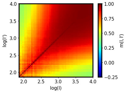
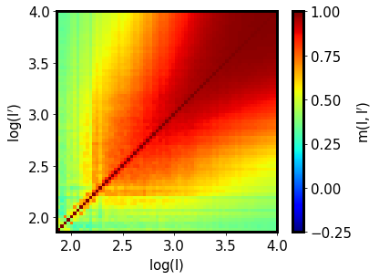
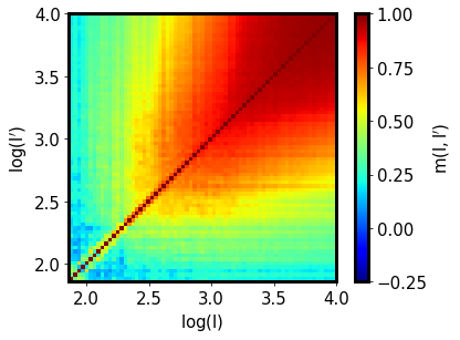
Figure 16: Same as Fig. 14 but considering in our convergence maps only the halo contributions: pinocchio plus wl-moka (only haloes). The three panels display the covariance matrix for sources at $z_{s}=0.5$, $1.4$ and $4$ from left to right, respectively.

Appendix B Convergence Maps at Different Grid Resolutions

In this section we display the convergence maps constructed adopting different particle and grid resolutions when running pinocchio while using the same seed and phases when displacing particles and haloes (3LPT) from the initial conditions. Fig. 17 shows the convergence map for sources at $z_{s}=1.4$; top left, bottom left and bottom right panels exhibit the results when running wl-moka on the PLC halo catalogues of the $1024^{3}$, $512^{3}$ and $2048^{3}$ pinocchio simulations, respectively. In all cases, we notice, the large scale structure is similar but the haloes have different displacements. The top right panel shows the convergence map constructed on the halo catalogue of the $1024^{3}$ run, but considering only systems more massive than $5.6\times 10^{12}M_{\odot}/h$, which corresponds to the halo mass resolution of the $512^{3}$. We recall for the reader that when building the convergence maps we assume the average to be zero (Hilbert et al., 2019) and that they are resolved with $2048\times 2048$ pixels on an angular scale of 5 deg on a side.

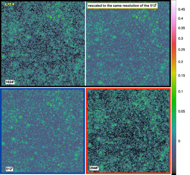
Figure 17: Convergence maps at $z_{s}=1.4$ for the same randomisation but for different runs. Top left, bottom left and bottom right display the convergence maps for the pinocchio runs with $1024^{3}$, $512^{3}$ and $2048^{3}$ particles, top right shows the convergence map build with running wl-moka on the $1024^{3}$ run but considering all haloes with mass larger than $5.6\times 10^{12}M_{\odot}/h$, which corresponds to the halo mass resolution of the $512^{3}$. In all cases we have adopted 3LPT displacement field and all maps are resolved with the same resolution of $2048\times 2048$ pixels on an angular scale of 5 deg by side.

In Fig. 18 we show the normalised Probability Distribution Function per pixel in the maps presented in Fig. 17. The different colours refer to the various runs and the arrows indicate the standard deviations of the distributions.

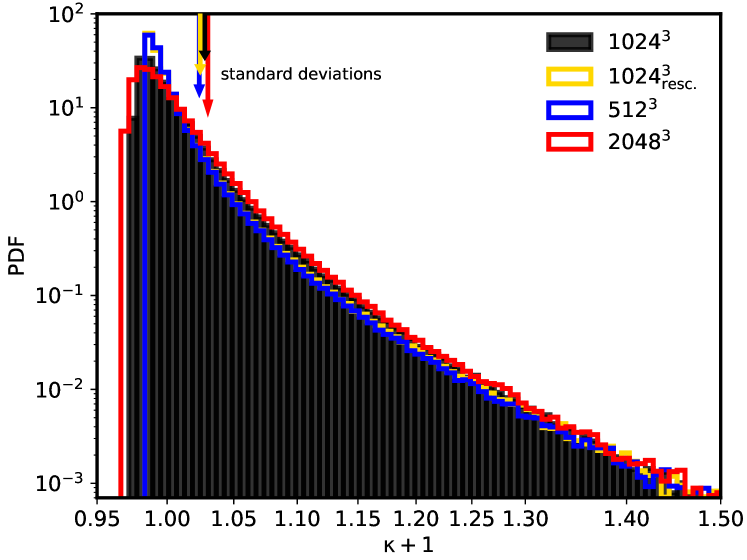
Figure 18: Probability Distribution Function per pixel of the convergence maps presented in Fig. 17. The arrows mark the standard deviation of the distributions, we recall the reader that by construction the maps have average equal to zero (Hilbert et al., 2019).

References

- Baldi (2012) Baldi M., 2012, MNRAS, 422, 1028
- Baldi et al. (2010) Baldi M., Pettorino V., Robbers G., Springel V., 2010, MNRAS, 403, 1684
- Barreira et al. (2018a) Barreira A., Krause E., Schmidt F., 2018a, J. Cosmology Astropart. Phys., 2018, 053
- Barreira et al. (2018b) Barreira A., Krause E., Schmidt F., 2018b, J. Cosmology Astropart. Phys., 2018, 015
- Bartelmann (1996) Bartelmann M., 1996, A&A, 313, 697
- Bartelmann & Schneider (2001) Bartelmann M., Schneider P., 2001, Physics Reports, 340, 291
- Baugh (2006) Baugh C. M., 2006, Reports on Progress in Physics, 69, 3101
- Benjamin et al. (2013) Benjamin J., Van Waerbeke L., Heymans C., Kilbinger M., Erben T., Hildebrandt H., Hoekstra H., et al. 2013, MNRAS, 431, 1547
- Bennett et al. (2013) Bennett C. L., Larson D., Weiland J. L., Jarosik N., Hinshaw G., Odegard N., Smith K. M., Hill R. S., et al. G., 2013, ApJS, 208, 20
- Bergamini et al. (2019) Bergamini P., Rosati P., Mercurio A., Grillo C., Caminha G. B., Meneghetti M., Agnello A., Biviano A., Calura F., Giocoli C., Lombardi M., Rodighiero G., Vanzella E., 2019, arXiv e-prints, p. arXiv:1905.13236
- Bernstein & Jarvis (2002) Bernstein G. M., Jarvis M., 2002, AJ, 123, 583
- Beutler et al. (2014) Beutler F., Saito S., Seo H.-J., Brinkmann J., Dawson K. S., Eisenstein D. J., Font-Ribera A., Ho S., McBride C. K., Montesano F., Percival W. J., Ross A. J., Ross N. P., Samushia L., Schlegel D. J., Sánchez A. G., Tinker J. L., Weaver B. A., 2014, MNRAS, 443, 1065
- Bond et al. (1991) Bond J. R., Cole S., Efstathiou G., Kaiser N., 1991, ApJ, 379, 440
- Bullock et al. (2001) Bullock J. S., Kolatt T. S., Sigad Y., Somerville R. S., Kravtsov A. V., Klypin A. A., Primack J. R., Dekel A., 2001, MNRAS, 321, 559
- Carbone et al. (2016) Carbone C., Petkova M., Dolag K., 2016, J. Cosmology Astropart. Phys., 7, 034
- Castorina et al. (2014) Castorina E., Sefusatti E., Sheth R. K., Villaescusa-Navarro F., Viel M., 2014, JCAP, 2, 49
- Castro et al. (2018) Castro T., Quartin M., Giocoli C., Borgani S., Dolag K., 2018, MNRAS, 478, 1305
- Chen et al. (2020) Chen Y., Mo H. J., Li C., Wang H., Yang X., Zhang Y., Wang K., 2020, arXiv e-prints, p. arXiv:2003.05137
- Cole et al. (2005) Cole S., Percival W. J., Peacock J. A., Norberg P., Baugh C. M., Frenk C. S., Baldry I., Bland-Hawthorn J., et al. 2005, MNRAS, 362, 505
- Cooray & Hu (2001) Cooray A., Hu W., 2001, ApJ, 554, 56
- Cooray & Sheth (2002) Cooray A., Sheth R., 2002, Physics Reports, 372, 1
- De Boni et al. (2016) De Boni C., Serra A. L., Diaferio A., Giocoli C., Baldi M., 2016, ApJ, 818, 188
- Debackere et al. (2019) Debackere S. N. B., Schaye J., Hoekstra H., 2019, MNRAS, p. 3078
- Despali et al. (2016) Despali G., Giocoli C., Angulo R. E., Tormen G., Sheth R. K., Baso G., Moscardini L., 2016, MNRAS, 456, 2486
- Dolag et al. (2004) Dolag K., Bartelmann M., Perrotta F., Baccigalupi C., Moscardini L., Meneghetti M., Tormen G., 2004, A&A, 416, 853
- Duffy et al. (2008) Duffy A. R., Schaye J., Kay S. T., Dalla Vecchia C., 2008, MNRAS, 390, L64
- Eisenstein et al. (2005) Eisenstein D. J., Zehavi I., Hogg D. W., Scoccimarro R., Blanton M. R., Nichol R. C., Scranton R., Seo H.-J., et al. 2005, ApJ, 633, 560
- Erben et al. (2013) Erben T., Hildebrandt H., Miller L., van Waerbeke L., Heymans C., Hoekstra H., Kitching T. D., et al. 2013, MNRAS, 433, 2545
- Fu et al. (2008) Fu L., Semboloni E., Hoekstra H., Kilbinger M., van Waerbeke L., Tereno I., Mellier Y., Heymans C., Coupon J., Benabed K., Benjamin J., Bertin E., Doré O., Hudson M. J., Ilbert O., Maoli et al. 2008, A&A, 479, 9
- Gao et al. (2008) Gao L., Navarro J. F., Cole S., Frenk C. S., White S. D. M., Springel V., Jenkins A., Neto A. F., 2008, MNRAS, 387, 536
- Giocoli et al. (2010) Giocoli C., Bartelmann M., Sheth R. K., Cacciato M., 2010, MNRAS, 408, 300
- Giocoli et al. (2017) Giocoli C., Di Meo S., Meneghetti M., Jullo E., de la Torre S., Moscardini L., Baldi M., Mazzotta P., Metcalf R. B., 2017, MNRAS, 470, 3574
- Giocoli et al. (2016) Giocoli C., Jullo E., Metcalf R. B., de la Torre S., Yepes G., Prada F., Comparat J., Göttlober S., Kyplin A., Kneib J.-P., Petkova M., Shan H. Y., Tessore N., 2016, MNRAS, 461, 209
- Giocoli et al. (2013) Giocoli C., Marulli F., Baldi M., Moscardini L., Metcalf R. B., 2013, MNRAS, 434, 2982
- Giocoli et al. (2012a) Giocoli C., Meneghetti M., Bartelmann M., Moscardini L., Boldrin M., 2012a, MNRAS, 421, 3343
- Giocoli et al. (2015) Giocoli C., Metcalf R. B., Baldi M., Meneghetti M., Moscardini L., Petkova M., 2015, MNRAS, 452, 2757
- Giocoli et al. (2007) Giocoli C., Moreno J., Sheth R. K., Tormen G., 2007, MNRAS, 376, 977
- Giocoli et al. (2018) Giocoli C., Moscardini L., Baldi M., Meneghetti M., Metcalf R. B., 2018, MNRAS
- Giocoli et al. (2012b) Giocoli C., Tormen G., Sheth R. K., 2012b, MNRAS, 422, 185
- Giocoli et al. (2010a) Giocoli C., Tormen G., Sheth R. K., van den Bosch F. C., 2010a, MNRAS, 404, 502
- Giocoli et al. (2008) Giocoli C., Tormen G., van den Bosch F. C., 2008, MNRAS, 386, 2135
- Guzzo et al. (2014) Guzzo L., Scodeggio M., Garilli B., Granett B. R., Fritz A., Abbas U., Adami C., Arnouts et al. 2014, A&A, 566, A108
- Harnois-Déraps et al. (2019) Harnois-Déraps J., Giblin B., Joachimi B., 2019, A&A, 631, A160
- Harnois-Déraps et al. (2012) Harnois-Déraps J., Vafaei S., Van Waerbeke L., 2012, MNRAS, 426, 1262
- Hartlap et al. (2007) Hartlap J., Simon P., Schneider P., 2007, A&A, 464, 399
- Hilbert et al. (2019) Hilbert S., Barreira A., Fabbian G., Fosalba P., Giocoli C., Bose S., Calabrese M., Carbone C., Davies C. T., Li B., Llinares C., Monaco P., 2019, arXiv e-prints, p. arXiv:1910.10625
- Hildebrandt et al. (2012) Hildebrandt H., Erben T., Kuijken K., van Waerbeke L., Heymans C., Coupon J., Benjamin J., et al. 2012, MNRAS, 421, 2355
- Hildebrandt et al. (2017) Hildebrandt H., Viola M., Heymans C., Joudaki S., Kuijken K., Blake C., Erben T., Joachimi B., et al. 2017, MNRAS, 465, 1454
- Hockney & Eastwood (1988) Hockney R. W., Eastwood J. W., 1988, Computer simulation using particles
- Ivezic et al. (2009) Ivezic Z., Tyson J. A., Axelrod T., Burke D., Claver C. F., Cook K. H., Kahn S. M., Lupton R. H., Monet D. G., Pinto P. A., Strauss M. A., Stubbs C. W., Jones L., Saha A., Scranton R., Smith C., LSST Collaboration 2009, in American Astronomical Society Meeting Abstracts #213 Vol. 41 of Bulletin of the American Astronomical Society, LSST: From Science Drivers To Reference Design And Anticipated Data Products. p. 366
- Izard et al. (2018) Izard A., Fosalba P., Crocce M., 2018, MNRAS, 473, 3051
- Jing (2000) Jing Y. P., 2000, ApJ, 535, 30
- Kacprzak et al. (2012) Kacprzak T., Zuntz J., Rowe B., Bridle S., Refregier A., Amara A., et al. 2012, MNRAS, 427, 2711
- Kilbinger (2015) Kilbinger M., 2015, Reports on Progress in Physics, 78, 086901
- Kilbinger et al. (2013) Kilbinger M., Fu L., Heymans C., Simpson F., Benjamin J., Erben T., Harnois-Déraps J., Hoekstra H., Hildebrandt H., et al. 2013, MNRAS, 430, 2200
- Kitching et al. (2014) Kitching T. D., Heavens A. F., Alsing J., Erben T., Heymans C., Hildebrandt H., Hoekstra H., et al. 2014, MNRAS, 442, 1326
- Kitching et al. (2019) Kitching T. D., Taylor P. L., Capak P., Masters D., Hoekstra H., 2019, arXiv e-prints, p. arXiv:1901.06495
- Knebe et al. (2011) Knebe A., Knollmann S. R., Muldrew S. I., Pearce F. R., Aragon-Calvo M. A., Ascasibar Y., Behroozi P. S., Ceverino D., et al. 2011, MNRAS, 415, 2293
- Köhlinger et al. (2017) Köhlinger F., Viola M., Joachimi B., Hoekstra H., van Uitert E., Hildebrandt H., Choi A., Erben T., Heymans C., Joudaki S., Klaes D., Kuijken K., Merten J., Miller L., Schneider P., Valentijn E. A., 2017, MNRAS, 471, 4412
- Komatsu et al. (2011) Komatsu E., Smith K. M., Dunkley J., Bennett C. L., Gold B., Hinshaw G., Jarosik N., Larson D., Nolta M. R., et al. 2011, ApJS, 192, 18
- Krause & Eifler (2017) Krause E., Eifler T., 2017, MNRAS, 470, 2100
- Labatie et al. (2012) Labatie A., Starck J. L., Lachièze-Rey M., 2012, ApJ, 760, 97
- Lacey & Cole (1993) Lacey C., Cole S., 1993, MNRAS, 262, 627
- Lange et al. (2019) Lange J. U., van den Bosch F. C., Zentner A. R., Wang K., Hearin A. P., Guo H., 2019, MNRAS, 490, 1870
- Laureijs et al. (2011) Laureijs R., Amiaux J., Arduini S., Auguères J. ., Brinchmann J., Cole R., Cropper M., Dabin C., Duvet L., et al. 2011, eprint arXiv: 1110.3193
- Lee et al. (2019) Lee S., Huff E. M., Ross A. J., Choi A., Hirata C., Honscheid K., MacCrann N., Troxel M. A., Davis C., et al. 2019, MNRAS, 489, 2887
- Lesgourgues & Pastor (2006) Lesgourgues J., Pastor S., 2006, Phys. Rep., 429, 307
- LSST Science Collaboration et al. (2009) LSST Science Collaboration Abell P. A., Allison J., Anderson S. F., Andrew J. R., Angel J. R. P., Armus L., Arnett D., Asztalos S. J., Axelrod T. S., et al. 2009, eprint arXiv: 0912.0201
- LSST Science Collaborations et al. (2009) LSST Science Collaborations Abell P. A., Allison J., Anderson S. F., Andrew J. R., Angel J. R. P., Armus L., Arnett D., Asztalos S. J., Axelrod T. S., et al. 2009, ArXiv e-prints
- Madau et al. (2008) Madau P., Diemand J., Kuhlen M., 2008, ApJ, 679, 1260
- Martinet et al. (2017) Martinet N., Schneider P., Hildebrandt H., Shan H., Asgari M., Dietrich J. P., Harnois-Déraps J., Erben T., Grado A., Heymans C., Hoekstra H., Klaes D., Kuijken K., Merten J., Nakajima R., 2017, ArXiv e-prints
- Marulli et al. (2013) Marulli F., Bolzonella M., Branchini E., Davidzon I., de la Torre S., Granett B. R., Guzzo L., Iovino et al. 2013, A&A, 557, A17
- Marulli et al. (2016) Marulli F., Veropalumbo A., Moresco M., 2016, Astronomy and Computing, 14, 35
- Massara et al. (2014) Massara E., Villaescusa-Navarro F., Viel M., 2014, J. Cosmology Astropart. Phys., 12, 053
- Meneghetti et al. (2008) Meneghetti M., Melchior P., Grazian A., De Lucia G., Dolag K., Bartelmann M., Heymans C., Moscardini L., Radovich M., 2008, A&A, 482, 403
- Meneghetti et al. (2014) Meneghetti M., Rasia E., Vega J., Merten J., Postman M., Yepes G., Sembolini F., Donahue M., Ettori S., Umetsu K., Balestra I., et al. 2014, ApJ, 797, 34
- Merten et al. (2015) Merten J., Meneghetti M., Postman M., Umetsu K., Zitrin A., Medezinski E., Nonino M., Koekemoer A., Melchior P., Gruen D., et al. 2015, ApJ, 806, 4
- Metcalf & Petkova (2014) Metcalf R. B., Petkova M., 2014, MNRAS, 445, 1942
- Miller et al. (2013) Miller L., Heymans C., Kitching T. D., van Waerbeke L., Erben T., Hildebrandt H., Hoekstra H., et al. 2013, MNRAS, 429, 2858
- Monaco et al. (2013) Monaco P., Sefusatti E., Borgani S., Crocce M., Fosalba P., Sheth R. K., Theuns T., 2013, MNRAS, 433, 2389
- Monaco et al. (2002) Monaco P., Theuns T., Taffoni G., 2002, MNRAS, 331, 587
- Montero-Dorta et al. (2020) Montero-Dorta A. D., Artale M. C., Abramo L. R., Tucci B., Padilla N., Sato-Polito G., Lacerna I., Rodriguez F., Angulo R. E., 2020, arXiv e-prints, p. arXiv:2001.01739
- Munari et al. (2017) Munari E., Monaco P., Sefusatti E., Castorina E., Mohammad F. G., Anselmi S., Borgani S., 2017, MNRAS, 465, 4658
- Navarro et al. (1996) Navarro J. F., Frenk C. S., White S. D. M., 1996, ApJ, 462, 563
- Neto et al. (2007) Neto A. F., Gao L., Bett P., Cole S., Navarro J. F., Frenk C. S., White S. D. M., Springel V., Jenkins A., 2007, MNRAS, 381, 1450
- Paranjape et al. (2013) Paranjape A., Sheth R. K., Desjacques V., 2013, MNRAS, 431, 1503
- Peacock & Dodds (1996) Peacock J. A., Dodds S. J., 1996, MNRAS, 280, L19
- Peebles (1980) Peebles P. J. E., 1980, The large-scale structure of the universe. Princeton University Press
- Peebles (1993) Peebles P. J. E., 1993, Principles of Physical Cosmology
- Percival et al. (2014) Percival W. J., Ross A. J., Sánchez A. G., Samushia L., Burden A., Crittenden R., Cuesta A. J., et al. 2014, MNRAS, 439, 2531
- Petkova et al. (2014) Petkova M., Metcalf R. B., Giocoli C., 2014, MNRAS, 445, 1954
- Planck Collaboration (2016) Planck Collaboration 2016, Astron. Astrophys., 594, A13
- Planck Collaboration et al. (2014) Planck Collaboration Ade P. A. R., Aghanim N., Alves M. I. R., Armitage-Caplan C., Arnaud M., Ashdown M., Atrio-Barandela F., Aumont J., Aussel H., et al. 2014, A&A, 571, A1
- Planck Collaboration et al. (2016) Planck Collaboration Ade P. A. R., Aghanim N., Arnaud M., Ashdown M., Aumont J., Baccigalupi C., Banday A. J., Barreiro R. B., Bartlett J. G., et al. 2016, A&A, 594, A24
- Postman et al. (2012) Postman M., Coe D., Benítez N., Bradley L., Broadhurst T., Donahue M., Ford H., Graur et al. 2012, ApJS, 199, 25
- Poulin et al. (2018) Poulin V., Boddy K. K., Bird S., Kamionkowski M., 2018, ArXiv e-prints: 1803.02474
- Prada et al. (2016) Prada F., Scóccola C. G., Chuang C.-H., Yepes G., Klypin A. A., Kitaura F.-S., Gottlöber S., Zhao C., 2016, MNRAS, 458, 613
- Ragagnin et al. (2019) Ragagnin A., Dolag K., Moscardini L., Biviano A., D’Onofrio M., 2019, MNRAS, 486, 4001
- Refregier et al. (2004) Refregier A., Massey R., Rhodes J., Ellis R., Albert J., Bacon D., Bernstein G., McKay T., Perlmutter S., 2004, AJ, 127, 3102
- Roncarelli et al. (2007) Roncarelli M., Moscardini L., Borgani S., Dolag K., 2007, MNRAS, 378, 1259
- Sánchez et al. (2014) Sánchez A. G., Montesano F., Kazin E. A., Aubourg E., Beutler F., Brinkmann J., Brownstein J. R., Cuesta A. J., et al. 2014, MNRAS, 440, 2692
- Sánchez et al. (2012) Sánchez A. G., Scóccola C. G., Ross A. J., Percival W., Manera M., Montesano F., Mazzalay X., Cuesta A. J., Eisenstein D. J., et al. 2012, MNRAS, 425, 415
- Sato & Nishimichi (2013) Sato M., Nishimichi T., 2013, Phys. Rev. D, 87, 123538
- Sawala et al. (2015) Sawala T., Frenk C. S., Fattahi A., Navarro J. F., Bower R. G., Crain R. A., Dalla Vecchia C., Furlong M., Jenkins A., McCarthy I. G., Qu Y., Schaller M., Schaye J., Theuns T., 2015, MNRAS, 448, 2941
- Schneider et al. (2019) Schneider A., Stoira N., Refregier A., Weiss A. J., Knabenhans M., Stadel J., Teyssier R., 2019, arXiv e-prints, p. arXiv:1910.11357
- Scoccimarro et al. (1999) Scoccimarro R., Zaldarriaga M., Hui L., 1999, ApJ, 527, 1
- Shan et al. (2018) Shan H., Liu X., Hildebrandt H., Pan C., Martinet N., Fan Z., Schneider P., Asgari M., et al. 2018, MNRAS, 474, 1116
- Sheth & Jain (2003) Sheth R. K., Jain B., 2003, MNRAS, 345, 529
- Sheth & Tormen (1999) Sheth R. K., Tormen G., 1999, MNRAS, 308, 119
- Sheth & Tormen (2004a) Sheth R. K., Tormen G., 2004a, MNRAS, 349, 1464
- Sheth & Tormen (2004b) Sheth R. K., Tormen G., 2004b, MNRAS, 350, 1385
- Simon et al. (2004) Simon P., King L. J., Schneider P., 2004, A&A, 417, 873
- Smith et al. (2003) Smith R. E., Peacock J. A., Jenkins A., White S. D. M., Frenk C. S., Pearce F. R., Thomas P. A., Efstathiou G., Couchman H. M. P., 2003, MNRAS, 341, 1311
- Somerville & Davé (2015) Somerville R. S., Davé R., 2015, ARA&A, 53, 51
- Springel (2005) Springel V., 2005, MNRAS, 364, 1105
- Takada & Jain (2004) Takada M., Jain B., 2004, MNRAS, 348, 897
- Takahashi et al. (2012) Takahashi R., Sato M., Nishimichi T., Taruya A., Oguri M., 2012, ApJ, 761, 152
- Tessore et al. (2015) Tessore N., Winther H. A., Metcalf R. B., Ferreira P. G., Giocoli C., 2015, J. Cosmology Astropart. Phys., 10, 036
- Tinker et al. (2008) Tinker J., Kravtsov A. V., Klypin A., Abazajian K., Warren M., Yepes G., Gottlöber S., Holz D. E., 2008, ApJ, 688, 709
- van den Bosch (2002) van den Bosch F. C., 2002, MNRAS, 331, 98
- Watson et al. (2013) Watson W. A., Iliev I. T., D’Aloisio A., Knebe A., Shapiro P. R., Yepes G., 2013, MNRAS, 433, 1230
- Wechsler et al. (2002) Wechsler R. H., Bullock J. S., Primack J. R., Kravtsov A. V., Dekel A., 2002, ApJ, 568, 52
- Wetzel et al. (2016) Wetzel A. R., Hopkins P. F., Kim J.-h., Faucher-Giguère C.-A., Kereš D., Quataert E., 2016, ApJ, 827, L23
- White & Rees (1978) White S. D. M., Rees M. J., 1978, MNRAS, 183, 341
- Wilkinson et al. (2004) Wilkinson M. I., Kleyna J. T., Evans N. W., Gilmore G. F., Irwin M. J., Grebel E. K., 2004, ApJl, 611, L21
- Wright et al. (2020) Wright A. H., Hildebrandt H., van den Busch J. L., Heymans C., Joachimi B., Kannawadi A., Kuijken K., 2020, arXiv e-prints, p. arXiv:2005.04207
- Yao et al. (2019) Yao J., Pedersen E. M., Ishak M., Zhang P., Agashe A., Xu H., Shan H., 2019, arXiv e-prints, p. arXiv:1911.01582
- Zehavi et al. (2019) Zehavi I., Kerby S. E., Contreras S., Jiménez E., Padilla N., Baugh C. M., 2019, ApJ, 887, 17
- Zehavi et al. (2011) Zehavi I., Zheng Z., Weinberg D. H., Blanton M. R., Bahcall N. A., Berlind A. A., Brinkmann J., Frieman et al. 2011, ApJ, 736, 59
- Zhao et al. (2009) Zhao D. H., Jing Y. P., Mo H. J., Bnörner G., 2009, ApJ, 707, 354
- Zhao et al. (2003b) Zhao D. H., Jing Y. P., Mo H. J., Börner G., 2003b, ApJ, 597, L9
- Zhao et al. (2003a) Zhao D. H., Mo H. J., Jing Y. P., Börner G., 2003a, MNRAS, 339, 12