Detecting Helium Reionization with Fast Radio Bursts

Abstract

Fast radio bursts (FRB) probe the electron density of the universe along the path of propagation, making high redshift FRB sensitive to the helium reionization epoch. We analyze the signal to noise with which a detection of the amplitude of reionization can be made, and its redshift, for various cases of future FRB survey samples, assessing survey characteristics including total number, redshift distribution, peak redshift, redshift depth, and number above the reionization redshift, as well as dependence on reionization redshift. We take into account scatter in the dispersion measure due to an inhomogeneous intergalactic medium (IGM) and uncertainty in the FRB host and environment dispersion measure, as well as cosmology. For a future survey with 500 FRB extending out to $z=5$, and a sudden reionization, the detection of helium reionization can approach the $5\sigma$ level and the reionization redshift be determined to $\sigma(z_{r})\approx 0.24$ in an optimistic scenario, or $2\sigma$ and $\sigma(z_{r})\approx 0.34$ taking into account further uncertainties on IGM fraction evolution and redshift uncertainties.

I Introduction

Reionization is one of the most dramatic processes in the young universe, turning the cosmic medium from its long, substantially neutral condition into an ionized state. For hydrogen atoms this occurs in the first billion years of the age of the universe, at redshifts $z\gtrsim 6$, and is a subject of extremely active research. A later epoch of reionization, more accessible to direct measurements by next generation surveys, is that of helium. While neutral helium loses its outer electron early, He II is believed to have its more tightly bound inner electron ionized when the universe is some two billion years old, at $z\approx 3$.

We refer to this later process simply as helium reionization, and relatively little is known about exactly when it occurs. Measurements of the event could shed light on energetic processes during this important epoch of the universe, when quasar black hole activity and star formation is nearing its peak. The addition of further free electrons to the intergalactic medium increases the optical depth to electromagnetic waves, and can be probed for example through the dispersion measure of fast radio bursts (FRB). The higher the electron density, the higher the plasma frequency for radio wave propagation, and the greater the frequency dispersion – quantified by the dispersion measure (DM) as an integral along the propagation path. For recent reviews of FRB, see 1906.05878 ; 1904.07947 . A very partial sample of some recent articles using FRB to learn about astrophysics and cosmology includes 1909.02821 ; kumlin ; 1903.06535 ; 1811.00899 ; 1811.00197 .

Here we investigate guidelines and early steps for assessing the ability of future FRB surveys to high redshift to detect helium reionization and estimate its characteristics. Section II describes the method and definition of a signal to noise for detection of the occurrence of helium reionization. We study the dependence of the results on survey characteristics such as number of sources, survey depth, redshift distribution, redshift peak, and number above the reionization redshift in Sec. III, as well as the role of IGM inhomogeneity and host galaxy DM uncertainty. The impact of further astrophysical or measurement uncertainties is considered in Sec. IV. We conclude in Sec. V.

II Dispersion Measure and Helium Reionization

We begin with a brief review of the key cosmological and astrophysical quantities entering the FRB measurements.

Fast radio bursts exhibit a characteristic sweep of the signal frequency with time, due to its propagation through an ionized medium. This can be characterized by its dispersion measure and interpreted as the integral along the line of sight of the electron density from emitter to observer. Thus,

$${\rm DM}=\int_{t_{e}}^{t_{o}}dt\,n_{e}(t)\,[1+z(t)]^{-1}\ ,$$ (1)

where the $1+z$ factor arises from frequency and time transformations between emitter and observer frames. The units are conventionally given as parsecs/cm³, though we will suppress explicitly writing them, as well as setting the speed of light to one.

The propagation time can be written in terms of the cosmological expansion rate, or Hubble parameter $H(z)$, as $dt=dz/[(1+z)H(z)]$, where $z$ is the redshift. Thus the cosmological model enters through $H(z)$, and if the electron density is well known then one could attempt to use FRB to constrain cosmology (e.g. 1903.06535 ; 1901.02418 ; 1812.11936 ; 1711.11277 , including a particular analysis of the effects of systematic uncertainties on cosmological parameter determination in kumlin ). Here we take the converse approach and seek to learn about the cosmic ionization history through $n_{e}(z)$ (see also 1808.00908 ; 1902.06981 ).

If the universe were perfectly homogeneous, and completely ionized for all redshifts of interest, then $n_{e}(z)=n_{e,0}(1+z)^{3}$ along every line of sight. However, the intergalactic medium is in fact inhomogeneous, giving a scatter to $n_{e}(z)$ at any specified redshift, and we are looking for signs of the helium reionization. Therefore we write $\langle n_{e}(z)\rangle=n_{e,0}(1+z)^{3}f_{e}(z)$ and consider the ionization history $f_{e}(z)$, while including variance in $n_{e}(z)$ at each redshift in the error budget.

We adopt the standard model for the ionization fraction, taking the universe to be made of a mass fraction $Y$ of helium and $1-Y$ of hydrogen. Since we will be considering surveys out to redshifts $z<6$, then we take all of the hydrogen to be ionized and none of the helium to be neutral (i.e. it is either singly ionized He II or fully ionized He III). In summary,

$$f_{e}(z)=(1-Y)f_{H}+\frac{Y}{4}(f_{\rm HeII}+2f_{\rm HeIII})\ ,$$ (2)

with the 2 accounting for He III having released 2 electrons to the cosmic medium. Thus, $f_{H}=1$, and before helium reionization $f_{\rm HeII}=1$ and $f_{\rm HeIII}=0$, while afterward $f_{\rm HeII}=0$ and $f_{\rm HeIII}=1$. Thus, $f_{e}(z>z_{r})=1-3Y/4=0.818$ and $f_{e}(z<z_{r})=1-Y/2=0.879$, where we take the Planck value of $Y=0.243$ planckhe (also see aver ). The ionization fraction increases by $\approx 7.5\%$ due to helium reionization. We assume the reionization occurs suddenly at redshift $z_{r}$ (though we later explore variations of this).

The dispersion measure due to cosmology (i.e. the propagation through the intergalactic medium) is therefore

$${\rm DM}=H_{0}^{-1}n_{e,0}\int_{z_{e}}^{z_{o}}\frac{dz\,(1+z)}{H(z)/H_{0}}\,f_{e}(z)\ .$$ (3)

The host galaxy of the FRB and its local environment also contribute to the detected dispersion measure. This is suppressed by a factor $1+z$, but we take it into account in our error budget. The Milky Way galaxy also gives rise to dispersion, but good maps exist to subtract this out ymw ; cordes . Therefore we take the “measured” value to be compared to theory to be simply given by Eq. (3).

The first question concerning helium reionization is whether we can detect it in a sample of high redshift FRB. Thus we want to explore a simple signal to noise criterion for detection. Beyond that we want to know when it occurs, i.e. estimate $z_{r}$. To accomplish this we adopt the form

$${\rm DM}(z)={\rm DM}(z)_{\rm high}+A_{He}\left[{\rm DM}(z)_{z_{r}}-{\rm DM}(z)_{\rm high}\right]\ .$$ (4)

Here the subscript “high” means reionization occurs beyond the limits of the sample, while the subscript “$z_{r}$” means it occurs at $z=z_{r}$. If $A_{He}=0$ then reionization is not detected by the sample, while if $A_{He}=1$ it is consistent with reionization occurring at $z_{r}$. Thus, if we determine $A_{He}$ to $\sigma(A_{He})$ then the detection signal to noise is $A_{He}/\sigma(A_{He})$, or simply $1/\sigma(A_{He})$ since $A_{He}=1$ if the model is correct.

Figure 1 illustrates the model and its effect on the cosmological DM. The cosmological DM has a significant change in slope with redshift due to the extra influx of electron density from helium reionization. The key questions are, first, can we detect this signature, i.e. find $A_{He}\neq 0$ with significant signal to noise, and can we measure the redshift $z_{r}$ at which reionization occurs. While the model curves appear close to each other, the signal to noise is enhanced by having many FRB over a wide redshift range on either side of the reionization redshift.

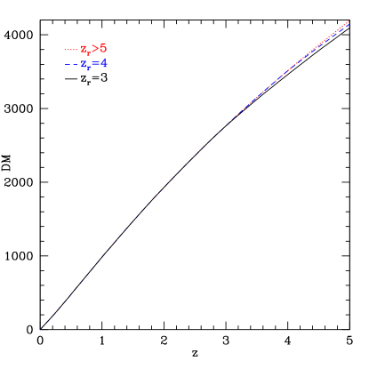
Figure 1: The cosmological DM has a clear change in slope at the reionization redshift. While the model with reionization occurring above the sample range (dotted red, with $z_{r}>5$) shows no special bend, the baseline model with $z_{r}=3$ (solid black) does. We also plot a case with higher than expected reionization redshift, $z_{r}=4$ (dashed blue).

We use the Fisher information matrix formalism to estimate the parameters $A_{He}$ and $z_{r}$, and include the cosmological parameter $\Omega_{m}$ (we assume a flat $\Lambda$CDM cosmology, where $H(z)/H_{0}$ is fully characterized by $\Omega_{m}$, the matter density as a fraction of the critical density). The fiducial values are taken to be $\Omega_{m}=0.3$, $A_{He}=1$, and $z_{r}=3$, though we will study the effect of different fiducial $z_{r}$ in the next section. Note that for the Fisher formalism the logarithmic derivatives of the measured quantity with respect to the fit parameters are the key elements, when the measurement errors dominate as we take here, so the constant prefactor in Eq. (3) is not important.

For the mock data, we use 500 FRB from a future survey, with redshifts, reaching out to $z_{\rm max}=5$. Our baseline FRB number density distribution with redshift increases at low redshift as the cosmic volume increases, then peaks around the expected helium reionization redshift, and declines at higher redshift due to diminished signal to noise. It is intended as a toy model, not a real survey distribution which would depend on detailed modeling of instrumental characteristics. To test sensitivity of the results to the survey we also compare to a distribution uniform with redshift; we do not find significant sensitivity to the exact form of the distribution. In Sec. III we also study the effect of variation of $z_{\rm max}$ and the peak redshift. In Sec. IV we discuss redshift uncertainties.

The error model for the DM “cleaned” measurements (i.e. with the contributions from within the Milky Way and host galaxy removed) includes scatter due to the inhomogeneous intergalactic medium (IGM), using the form kumlin

$$\frac{\sigma({\rm DM})_{\rm IGM}}{{\rm DM}_{\rm IGM}}=\frac{20\%}{\sqrt{z}}\ ,$$ (5)

inspired by simulations 1309.4451 ; 1812.11936 ; 1712.01280 ; 1901.11051 . The host and local environment contributions to the detected DM may be random among the FRB sample; we do not actually need the value of the mean of those noncosmological fluctuations for our analysis (i.e. the value that will be subtracted off to define the cosmological contribution) only the residual scatter that will presumably be random and hence reduced by $\sqrt{N}$ using $N$ FRB. This is not well known; we assume a residual uncertainty $\sigma({\rm DM})_{\rm host}\approx 30$ (redshift independent, i.e. $30(1+z)$ in the host frame, reflecting greater uncertainty at higher redshift), but study the effects of varying this.

Figure 2 shows the baseline and uniform distributions of FRB in our mock surveys. The baseline form is

$$n_{\rm FRB}(z)\sim z^{3}\,e^{-z/z_{\star}}\ ,$$ (6)

and the uniform one is $n(z)=\,$const, both normalized to give 500 FRB from $z=[0,z_{\rm max}]$. Fiducial values are $z_{\rm max}=5$, $z_{\star}=1$, though we later vary these.

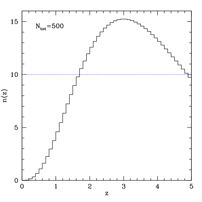
Figure 2: The mock FRB sample distribution is shown in redshift bins of width 0.1 for the baseline (solid black) and uniform (dotted blue) distributions. Both contain 500 FRB.

Figure 3 shows the model for the fractional uncertainty on an individual cosmological DM measurement, accounting for scatter in IGM properties and host and local environment variations. Since DM is small at low redshift, the fractional uncertainty is large there. At higher redshift, lines of sight average over IGM inhomogeneity, and DM increases, so the fractional uncertainty decreases. The host and local environment residual contribution is much smaller than the IGM uncertainty – for example at $z=1$ the IGM DM scatter is $\approx 210$, so adding the host uncertainty of 30 (not DM_host) in quadrature gives negligible increase. We also show the effect of increasing the host uncertainty to 100; it is still not a large effect, especially near the expected reionization redshift $z_{r}\gtrsim 3$.

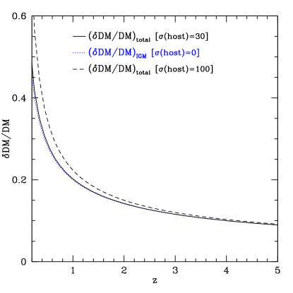
Figure 3: The fractional uncertainty contributing to a measured DM, due to IGM scatter and uncertainty in the host and local environment contribution, is plotted vs redshift. The quadrature sum of the two contributions is plotted as the solid black curve, using a baseline host uncertainty $\delta{\rm DM}=30$, while using an increased host uncertainty of 100 is shown by the dashed black curve. The dotted blue curve gives the IGM scatter contribution alone. In the high redshift region with the most information on helium reionization the IGM component dominates.

III Results and Survey Dependence

Having all the elements in place, we can now use the Fisher information analysis to evaluate the parameter estimation. For our baseline case we find the marginalized parameter uncertainties are $\sigma(A_{He})=0.22$ and $\sigma(z_{r})=0.24$. That is, the signal to noise for detection, $S/N=A_{He}/\sigma(A_{He})=1/\sigma(A_{He})=4.5$. Furthermore, we can constrain the sudden reionization model to have $z_{r}=3\pm 0.24$. Since all the input errors are treated statistically, all uncertainties will scale as $1/\sqrt{N}$. (Recall we use $N=500$.)

There is not a strong covariance between $A_{He}$ and $z_{r}$ determinations, and they are not especially sensitive to the difference between the baseline and uniform FRB distributions. (At the end of this section we also investigate further the role of $z_{\rm max}$ and the distribution peak $z_{\rm peak}=3z_{\star}$.) For example, the parameter uncertainties increase to 0.28 and 0.33, respectively. Figure 4 shows the 68.3% ($1\sigma$) joint confidence contours.

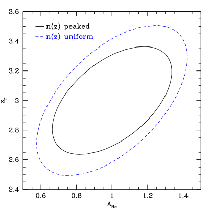
Figure 4: 68.3% ($1\sigma$) joint confidence contours on the reionization parameters $A_{He}$ and $z_{r}$ are plotted for the baseline FRB distribution (“peaked”: solid black) and uniform distribution (dashed blue). Such FRB samples would clearly enable distinction from $A_{He}=0$, i.e. detection of helium reionization within the sample redshift range, and reasonable localization of $z_{r}$.

We can explore the sensitivity as we vary the reionization redshift. Figure 5 shows that the S/N increases appreciably for lower $z_{r}$, but fades below $S/N=1$ for $z_{r}\gtrsim 4$. The uncertainty $\sigma(z_{r})$ has a slower dependence, though it becomes steeper as one approaches the edge of the sample. Over the main part of the expected range, say $z_{r}\approx 2.5$–3.5, the S/N varies between 6.2 and 2.7, and $\sigma(z_{r})$ between 0.22 and 0.29.

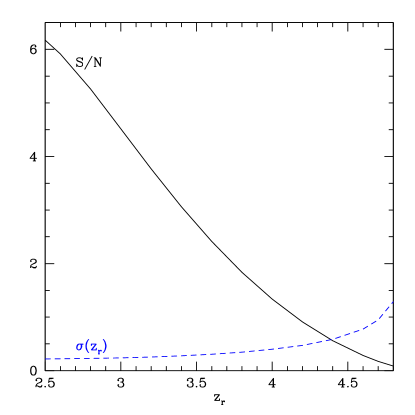
Figure 5: The signal to noise $S/N=1/\sigma(A_{He})$ for detection of reionization and the uncertainty on the reionization redshift $\sigma(z_{r})$ are plotted vs the value of $z_{r}$. As one approaches the sample edge at $z_{\rm max}=5$, the S/N vanishes and the redshift uncertainty blows up.

If we assume our model is correct, i.e. sudden reionization at $z_{r}$ does occur within the sample range, and fix $A_{He}=1$, then the uncertainty $\sigma(z_{r})$ only decreases from 0.24 to 0.20 for the fiducial case $z_{r}=3$. This is due to the lack of strong covariance between $A_{He}$ and $z_{r}$.

One could also relax the assumption of sudden reionization and attempt to see a signal of a more gradual transition. This will correspond to finding (e.g. within a Monte Carlo parameter estimation) a fit value of $A_{He}\neq 1$. Using Eqs. (2)–(4) one finds that one can write

$$A_{He}(z)=1-\frac{\int_{z_{r}}^{z}\frac{dz^{\prime}\,(1+z^{\prime})}{H(z^{\prime})/H_{0}}\,f_{\rm HeIII}(z)}{\int_{z_{r}}^{z}\frac{dz^{\prime}\,(1+z^{\prime})}{H(z^{\prime})/H_{0}}}\ .$$ (7)

That is, $A_{He}$ is (one minus) a weighted ionization fraction. For sudden reionization this reduces to what we use throughout this article. Thus a fit value $A_{He}$ statistically distinct from one or zero would point to a gradual reionization process, where $f_{\rm HeIII}$ does not suddenly transition from zero to one. That serves as an alert that, while reionization is detected, one should carry out an analysis with a redshift dependent function rather than a single constant parameter $A_{He}$ (for example a principal components analysis as in hu1 ; hu2 ).

We can check the robustness of the results for other variations in the inputs. If we change the host uncertainty contribution from 30 to 10 or 100, then $\sigma(A_{He})$ goes from 0.22 to 0.22 or 0.23, respectively, and $\sigma(z_{r})$ from 0.24 to 0.24 or 0.25.

Increasing the sample depth $z_{\rm max}$ will certainly decrease the parameter uncertainties, but it is fairer to do so while holding the total number of FRB fixed. As seen in Fig. 6, in this case the S/N gets worse rapidly with decreased depth, due to the reduced lever arm above the reionization redshift. However the localization of the bend in DM, i.e. $\sigma(z_{r})$ stays fairly constant until the sample depth approaches $z_{r}$ (where one loses leverage above $z_{r}$).

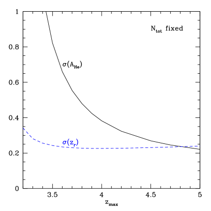
Figure 6: Changing the depth of the FRB sample, $z_{\rm max}$, has a significant effect on the inverse S/N, $\sigma(A_{He})$ (solid black curve), but less on the reionization redshift uncertainty (dashed blue). Here we hold the total number of FRB fixed as we change $z_{\rm max}$, keeping the form of the redshift distribution the same.

We can also change how the FRB distribution out to the fiducial $z_{\rm max}=5$ is shaped. The peak of the distribution in Eq. (6) occurs at $z_{\rm peak}=3z_{\star}$. We can either keep the total number of FRB fixed, or the number of FRB with $z>z_{r}$ fixed. Our fiducial case has 500 total FRBs, of which 260, or just about half are at $z>z_{r}$. Fixing $N(z>z_{r})$ is interesting since we might expect the leverage on the reionization parameters to come from the different behavior at $z>z_{r}$ before reionization, i.e. DM($z<z_{r}$) does not depend on $A_{He}$ or $z_{r}$.

Figure 7 shows that this is indeed so. If we fix $N_{\rm tot}$, then moving the peak of the distribution to lower redshifts worsens the uncertainty on $A_{He}$, i.e. it becomes harder to be sure that reionization occurred at all (the S/N drops below 2 for $z_{\rm peak}=1.8$; note there are then only 120 FRB above $z_{r}$). However, fixing the number above $z_{r}$ instead greatly ameliorates this effect, nearly leveling out $\sigma(A_{He})$ despite the change in $z_{\rm peak}$. For $\sigma(z_{r})$, however, while peaking the distribution at low redshift worsens its estimation, this is completely overturned when fixing $N(z>z_{r})$ because there are also many more total FRB; for $z_{\rm peak}=1.8$ there are then 1087 total FRB in the full distribution.

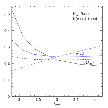
Figure 7: Changing the shape of the FRB distribution, here quantified in terms of the peak redshift, does not have a large effect on the parameter estimation ($A_{He}$ in black, $z_{r}$ in light blue) as long as the range on either side of the reionization redshift is reasonably sampled. Solid curves show the case where the total number of FRB in the full distribution is held fixed, while dashed curves preserve the number of FRB above the reionization redshift.

IV Further Uncertainties

In using Eq. (3) to account for the effect of helium reionization on the electron number density, we assumed that all free electrons contributed to the intergalactic medium. However, this is not completely true and one often includes a factor $f_{\rm IGM}$ in the equation representing the fraction present in the IGM. To the extent that this is constant with redshift, it can be absorbed in the other constant factors and does not affect the results so far. However, a modest ($\sim 20\%$) evolution is expected over the range $z=0$–5 (see, e.g., 1309.4451 ; 1901.11051 ; 1909.02821 ), though slower around the range of redshifts of interest for helium reionization shull12 ; 1812.11936 . We here write

$$f_{\rm IGM}(z)=f_{\rm IGM}(z=3)\,[1+s(z-3)]\ ,$$ (8)

and add $s$ as a fit parameter.

We then incorporate the slope $s$ into the Fisher information analysis and assess the impact on the parameter uncertainties. Figure 8 shows the results (for this case and the others in this section). Here we focus on the effect of including $f_{\rm IGM}(z)$, corresponding to going from the solid black contour (the same as in Fig. 4) to the dashed blue contour. The uncertainty on $A_{He}$ increases from 0.22 to 0.40, changing the “detection” S/N from 4.5 to 2.5. Essentially the evolution of the IGM fraction blurs the bend due to helium reionization; of course for a free function $f_{\rm IGM}(z)$ one could exactly offset the change in the ionization fraction.

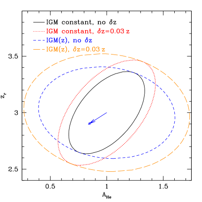
Figure 8: 68.3% ($1\sigma$) joint confidence contours on the reionization parameters $A_{He}$ and $z_{r}$ are plotted for the baseline FRB distribution as in Fig. 4 (solid black) and with various additional uncertainties. Allowing linear evolution of the IGM fraction $f_{\rm IGM}(z)$ gives the dashed blue contour, while including redshift uncertainty as a contribution to the measurement covariance matrix yields the dotted red contour. Adding both gives the long dashed orange contour. Treating redshift errors as a systematic offset will bias the astrophysics results by changing their values as shown by the blue arrow giving the shift in the center of the dashed blue contour.

Another uncertainty is the FRB redshift. Localization to a specific galaxy can be a challenge, especially at high redshift. One can also take a statistical approach by crosscorrelating with large scale structure in the uncertainty volume. What we are interested in is not individual redshifts per se, but rather the uncertainty of estimation over a number of FRB within a redshift bin. The central limit theorem helps in that even if individual redshift probability distributions may be non-Gaussian, the ensemble estimate should be Gaussian. We want the uncertainty in that estimation. This is a common issue in cosmological distance estimation, e.g. from supernovae without spectroscopic redshifts or gravitational wave standard sirens.

We approach it in two ways: in the first method we include an ensemble redshift uncertainty in the measurement noise matrix, added in quadrature with the other uncertainties, while in the second method we use the Fisher bias formalism (see snbias for its application to photometric supernovae, gwbias for its application to standard sirens, and kumlin for its application using a different uncertainty to FRB).

For the first, statistical method we add

$$\left[\delta z\frac{\partial{\rm DM}(z_{i})}{\partial z}\right]^{2}$$ (9)

to the noise matrix, taking each bin $i$ independently. We adopt an uncertainty $\delta z=\alpha z$, with $\alpha=0.03$. This increases the uncertainty on the astrophysical parameter estimation, specifically diluting the $A_{He}$ determination from 0.22 to 0.28, and $\sigma(z_{r})$ from 0.24 to 0.31. This is shown in Fig. 8 for both the redshift uncertainty alone, and in combination with the previous IGM evolution uncertainty where the parameter uncertainties increase to 0.48 and 0.34 respectively.

For the second, systematic uncertainty we instead apply $\delta z=\alpha z$, again with $\alpha=0.03$, as a systematic offset to each redshift bin. The shift in the confidence contour central values, for the case including IGM evolution as well, is denoted by the blue arrow in Fig. 8. We can assess the impact of the shift by taking into account the joint bias between $A_{He}$ and $z_{r}$ (i.e. direction as well as magnitude) in terms of the $\Delta\chi^{2}$ shifted. The value for $\alpha=0.03$ (and it scales quadratically with $\alpha$ for small bias) is $\Delta\chi^{2}=0.3$. Since the $1\sigma$ joint confidence contour lies at $\Delta\chi^{2}=2.3$, this can be thought of as a $0.14\sigma$ joint shift. Thus, redshift uncertainties at the 0.03 level (for the redshift bin ensemble, not individual FRB) are not very significant, whether treated through the statistical or systematic approach.

V Conclusions

Helium reionization is an important transition in the evolution of the cosmic medium, and bears potential clues to quasar black hole activity, star formation, and baryon distribution. Fast radio bursts have, well, burst onto the scene as a promising tool for probing the intergalactic medium to these redshifts.

Future surveys will have many thousands of FRB detections, and new telescopes offer the possibility of tight localization. While identification of counterpart galaxies, and redshifts, may be more challenging at high redshift, new ideas such as Ultra-Fast Astronomy ufa in the optical may help. An alternative approach is statistical crosscorrelation with large scale structure to obtain redshifts. Here we considered 500 FRB with redshifts out to $z\approx 5$, though we discussed the scaling of results with numbers and depth.

We explored guidelines for where lay the greatest leverage in survey characteristics, assessing total number, redshift distribution, peak redshift, redshift depth, and number above the reionization redshift. The last was identified as the most important variable (though it is important to have a lever arm on both sides of the helium reionization epoch). We also examined how the value of the reionization redshift $z_{r}$ affected prospects for detection and found the effect was modest within the expected redshift range.

Defining a signal to noise criterion for detecting helium reionization, we carried out a Fisher information analysis to estimate constraints on the S/N and the redshift of reionization. We included uncertainties due to a inhomogeneous IGM, host galaxy contributions, and cosmology (within $\Lambda$CDM). For 500 FRB, roughly half above and half below the reionization redshift, the detection S/N $\approx 4.5$ and $\sigma(z_{r})\approx 0.24$. A value of the “reionizationness” $A_{He}<1$ could be interpreted as a weighted reionization fraction $1-\langle f_{\rm HeIII}\rangle$ that indicates a more gradual transition than instantaneous reionization. These calculations are early steps and guidelines toward future work using more sophisticated simulations of IGM properties and potential methods for reducing uncertainty in the IGM and host contributions.

We also investigated systematics in terms of evolution in the IGM fraction, finding that it could significantly weaken detection of reionization, so that complementary observations that could constrain this (e.g. through X-ray, Sunyaev-Zel’dovich, or neutral hydrogen measurements) could play an important role. Uncertainties in FRB redshifts were accounted for in two ways: treating them as a statistical uncertainty “bloating” the parameter estimation or as a systematic bias. In both cases, if the redshift uncertainty can be controlled at the $\sim 3\%$ fractional level then parameter estimation is not seriously degraded.

Whether obtaining such a large sample of FRB, with well estimated redshifts, at such high redshift is realistic or not is difficult to foretell. However the extraordinary rapid development of FRB detections in the last couple of years argues that consideration of the possibilities for such a sample to explore the cosmic medium should not be neglected.

- (1) J.M. Cordes, S. Chatterjee, Fast Radio Bursts: An Extragalactic Enigma, Ann. Rev. Astron. Astroph. 57, 417 (2019) [arXiv:1906.05878]
- (2) E. Petroff, J.W.T. Hessels, D.R. Lorimer, Fast Radio Bursts, Astron. Astroph. Rev. 27, 4 (2019) [arXiv:1904.07947]
- (3) A. Walters, Y-Z. Ma, J. Sievers, A. Weltman, Probing Diffuse Gas with Fast Radio Bursts, Phys. Rev. D 100, 103519 (2019) [arXiv:1909.02821]
- (4) P. Kumar, E.V. Linder, Use of Fast Radio Burst Dispersion Measures as Distance Measures, Phys. Rev. D 100, 083533 (2019) [arXiv:1903.08175]
- (5) V. Ravi et al., Fast Radio Burst Tomography of the Unseen Universe, arXiv:1903.06535
- (6) E.F. Keane, The Future of Fast Radio Burst Science, Nature Ast. 2, 865 (2018) [arXiv:1811.00899]
- (7) J-P. Macquart, Probing the Universe’s baryons with fast radio bursts, Nature Ast. 2, 836 (2018) [arXiv:1811.00197]
- (8) M.S. Madhavacheril, N. Battaglia, K.M. Smith, J.L. Sievers, Cosmology with kSZ: breaking the optical depth degeneracy with Fast Radio Bursts, Phys. Rev. D 100, 103532 (2019) [arXiv:1901.02418]
- (9) M. Jaroszynski, Fast Radio Bursts and cosmological tests, MNRAS 484, 1637 (2019) [arXiv:1812.11936]
- (10) A. Walters, A. Weltman, B.M. Gaensler, Y-Z. Ma, A. Witzemann, Future Cosmological Constraints from Fast Radio Bursts, ApJ 856, 65 (2018) [arXiv:1711.11277]
- (11) J-P. Macquart, R.D. Ekers, FRB event rate counts II – fluence, redshift and dispersion measure distributions, MNRAS 480, 4211 (2018) [arXiv:1808.00908]
- (12) M. Caleb, C. Flynn, B. Stappers, Constraining the era of helium reionization using fast radio bursts, MNRAS 485, 2281 (2019) [arXiv:1902.06981]
- (13) Planck Collaboration, Planck 2018 results. VI. Cosmological parameters, arXiv:1807.06209
- (14) E. Aver, K.A. Olive, E.D. Skillman, The effects of He I 10830 on helium abundance determinations, JCAP 1507, 011 (2015) [arXiv:1503.08146]
- (15) J.M. Yao, R.N. Manchester, N. Wang, A New Electron Density Model for Estimation of Pulsar and FRB Distances, ApJ 835, 29 (2017) [arXiv:1610.09448]
- (16) J.M. Cordes, T.J.W. Lazio, NE2001.I. A New Model for the Galactic Distribution of Free Electrons and its Fluctuations, arXiv:astro-ph/0207156
- (17) M. McQuinn, Locating the “missing” baryons with extragalactic dispersion measure estimates, ApJ 780, L33 (2014) [arXiv:1309.4451]
- (18) J.M. Shull, C.W. Danforth, The Dispersion of Fast Radio Bursts from a Structured Intergalactic Medium at Redshifts , ApJL 852, L11 (2018) [arXiv:1712.01280]
- (19) J.X. Prochaska and Y. Zheng, Probing Galactic haloes with fast radio bursts, MNRAS 485, 648 (2019) [arXiv:1901.11051]
- (20) W. Hu, G. Holder, Model-Independent Reionization Observables in the CMB, Phys. Rev. D 68, 023001 (2003) [arXiv:astro-ph/0303400]
- (21) M.J. Mortonson, W. Hu, Model-independent constraints on reionization from large-scale CMB polarization, ApJ 672, 737 (2008) [arXiv:0705.1132]
- (22) J.M. Shull, B.D. Smith, C.W. Danforth, The Baryon Census in a Multiphase Intergalactic Medium: 30% of the Baryons May Still Be Missing, ApJ 759, 23 (2012) [arXiv:1112.2706]
- (23) E.V. Linder, A. Mitra, Photometric Supernovae Redshift Systematics Requirements, Phys. Rev. D 100, 043542 (2019) [arXiv:1907.00985]
- (24) R.E. Keeley, A. Shafieloo, B. L’Huillier, E.V. Linder, Debiasing Cosmic Gravitational Wave Sirens, MNRAS 491, 3983 (2020) [arXiv:1905.10216]
- (25) S. Li, G.F. Smoot, B. Grossan, A.W.K. Lau, M. Bekbalanova, M. Shafiee, T. Stezelberger, Program objectives and specifications for the Ultra-Fast Astronomy observatory, Proc. SPIE 11341, 113411Y (2019) [arXiv:1908.10549]