The OTELO survey

Abstract

Context. The evolution of galaxies through cosmic time is studied observationally by means of extragalactic surveys. The usefulness of these surveys is greatly improved by increasing the cosmological volume, in either depth or area, and by observing the same targets in different wavelength ranges. A multi-wavelength approach using different observational techniques can compensate for observational biases.

Aims. The OTELO survey aims to provide the deepest narrow-band survey to date in terms of minimum detectable flux and emission line equivalent width in order to detect the faintest extragalactic emission line systems. In this way, OTELO data will complements other broad-band, narrow-band, and spectroscopic surveys.

Methods. The red tunable filter of the OSIRIS instrument on the 10.4 m Gran Telescopio Canarias (GTC) is used to scan a spectral window centred at 9175 Å, which is free from strong sky emission lines, with a sampling interval of 6 Å and a bandwidth of 12 Å in the most deeply explored EGS region. Careful data reduction using improved techniques for sky ring subtraction, accurate astrometry, photometric calibration, and source extraction enables us to compile the OTELO catalogue. This catalogue is complemented with ancillary data ranging from deep X-ray to far-infrared, including high resolution HST images, which allow us to segregate the different types of targets, derive precise photometric redshifts, and obtain the morphological classification of the extragalactic objects detected.

Results. The OTELO multi-wavelength catalogue contains 11 237 entries and is 50% complete at AB magnitude 26.38. Of these sources, 6600 have photometric redshifts with an uncertainty $\delta\,$z${}_{\rm\,phot}$ better than 0.2 (1+z${}_{\rm\,phot}$). A total of 4336 of these sources correspond to preliminary emission line candidates, which are complemented by 81 candidate stars and 483 sources that qualify as absorption line systems. The OTELO survey data products were released to the public on 2019.

1 Introduction

Extragalactic surveys are an essential tool for studying galaxy evolution. Considerable amounts of observing time have been invested, mainly in the last few decades, in gathering deeper and larger datasets, enriched with observations covering wide wavelength ranges, through the use of different instruments covering the same areas of sky.

Imaging surveys using broad-band filters, with passbands of the order of 100 nm or more, detect the faintest objects, per unit observing time and telescope aperture, at the price of losing spectral resolution. However, the development of such photometric redshift tools as LePhare (Arnouts et al., 1999; Ilbert et al., 2006), Zebra (Feldmann et al., 2006), BPZ (Benítez et al., 2004), and other SED-fitting facilities has somewhat alleviated this limitation. Moreover, high spatial resolution broad- band surveys allow the determination of galaxy morphologies, an essential parameter for studying galaxy evolution. The large number of existing or planned surveys of this kind makes it difficult to provide a reasonably complete compilation, but the Hubble Deep Field (Williams et al., 1996), including its southern, flanking, and deep extensions, SDSS (York et al., 2000), COSMOS (Scoville et al., 2007), VVDS (Le Fèvre et al., 2004a), and CANDELS (Grogin et al., 2011) give a hint of the importance of broad-band surveys.

The first attempts at obtaining better spectral resolutions in extragalactic surveys were based on slitless blind spectroscopy. KISS (Wegner et al., 2003), UCM (Gallego et al., 1993), CUYS (Bongiovanni et al., 2005), and more recently PEARS (Straughn et al., 2009) are representative examples. They are hampered by spectra overlapping in crowded fields, especially in the case of extended sources. These limitations has been overcome with the advent of multi-plexing spectroscopic techniques (via multiple slits, integral field units, and image slicers). In this case, broad-band surveys provide the slit or fibre positions required for spectroscopic surveys, either blind or with target pre-selection, using the same broad-band or other ancillary data. The spectral resolution provided and the rich physical information that can then be derived compensate for the lower limiting magnitude, with respect to imaging, that can be reached with these kinds of surveys. Worth mentioning are SDSS (York et al., 2000), GAMA (Driver et al., 2011), z-COSMOS (Lilly et al., 2007), DEEP2 (Newman et al., 2013), and VVDS-CFDS (Le Fèvre et al., 2004b). For a more detailed compilation of spectroscopic surveys of galaxies at $z\leqslant 2$ see Hayashi et al. (2018).

Mid-band surveys, with filter passbands of the order of ten to a few tens of nm, possibly with some overlapping of contiguous filters covering a relatively wide spectral band, represent an intermediate situation between the depth achieved in imaging, and the spectral coverage and resolution achieved in spectroscopy. They are advantageous when the number of sources in the field is so large that the amount of time invested in observing through a large number of filters is comparable to, or lower than, what should be spent in gathering spectroscopic information (Benítez et al., 2014). This situation can be achieved by either by the depth or the angular coverage of the survey. COMBO-17 (Wolf et al., 2003), ALHAMBRA (Moles et al., 2008), J-PAS (Benítez et al., 2014), and SHARDS (Pérez-González et al., 2013), are some recent examples of this kind of survey.

Narrow band imaging surveys use passbands of the order of 10 nm or lower and are usually designed to reach the maximum depth in a wavelength range restricted by the filter response. They target mainly emission line candidates, identified using colour–magnitude diagrams (see for example Thompson et al., 1995; Pascual et al., 2007; Ota et al., 2010). Different redshift ranges are explored, defined by the emission line detected, and the wavelength range is defined by the filter. For a complete review of the narrow-band surveys performed so far, see Hayashi et al. (2018).

One particular type of narrow-band imaging survey uses tunable filters (TFs) instead of standard fixed-cavity interference filters (see for example Glazebrook et al., 2004). TFs define narrower passbands, of the order of 1 nm up to a few nm (Atherton & Reay, 1981). This allows the study of lower equivalent width (EW) emission features because the passband of the filter is related to the EW of the emission lines that can be detected. This effect can be estimated using the contrast parameter defined in Thompson et al. (1995) and is explicitly acknowledged in, for example, the ongoing fixed-cavity standard narrow-band survey HSC-SSP (Hayashi et al., 2018), which uses narrow band filters of 113 and 135 Å. A practical example of the lower EW bound reached in OTELO can be seen in Ramón-Pérez et al. (2019), hereafter referred as OTELO-II. However, this advantage is usually at the price of requiring several images at different wavelengths with some overlapping between them (see for example Jones & Bland-Hawthorn, 2001) to increase emission line identification and improve flux accuracy (Lara-López et al., 2010). Another advantage of TF surveys is that they allow the detection of the faintest emission line targets with low continuum, which are probably missed in broad-band, and hence spectroscopic, surveys. Jones & Bland-Hawthorn (2001) pointed out that there is little overlap between emission-line selected galaxies (hereafter, emission line source or ELS) found in broad-band selected redshift surveys and TF surveys. The effect of the bandpass width and transmission profile of narrow- band filters on the finding of Ly$\alpha$ emitter (LAE) candidates at redshift z $\sim$ 6.5, was studied by de Diego et al. (2013) in a pilot survey to test the performance of TFs to find this and other emission-line candidates. They anticipated that fixed-cavity standard narrow-band filter surveys underestimate the number counts of LAEs and other emitters, when the observed EW $\lesssim 60$ Å. Such bias can be largely mitigated using TFs such as that of the OTELO survey. TTF (Bland-Hawthorn & Jones, 1998), CADIS (Hippelein et al., 2003), and more recently GLACE (Sánchez-Portal et al., 2015) are examples of narrow-band surveys using TFs. GLACE has been conducted mainly by members of the OTELO team and benefits from OTELO observing strategies, whereas OTELO uses certain GLACE data analysis approaches.

This is the first of a series of papers devoted to the OSIRIS Tunable Filter Emission Line Object (OTELO) survey, a pencil-beam probe designed for finding faint ELSs at different comoving volumes up to redshift z $\sim 6.5$ through the exploitation of the red TF of the OSIRIS instrument on the GTC. The data gathering and reduction and the construction of the OTELO multi-wavelength catalogue are described here. This article includes a first selection of ELS candidates and a study of their properties. The second article of the series (OTELO-II) and subsequent contributions about this survey set forth the techniques adopted for the study of pre-selected collections of ELSs based on OTELO low-resolution spectra, and a science case example as a demonstration of the survey potential. In the calculations carried out this paper we assume a standard $\Lambda$-cold dark matter cosmology with $\Omega_{\Lambda}$=0.69, $\Omega_{\rm m}$=0.31, and $H_{0}$=67.8 km s^-1 Mpc^-1, as extracted from Planck Collaboration XIII (2016).

2 The OTELO survey

OTELO is a very deep, 2D spectroscopic (resolution $R\sim 700$) blind survey, defined on a window of 230 ${\rm\AA}$, centred at 9175 ${\rm\AA}$. The first pointing of OTELO targets a region of the Extended Groth Field embedded in Deep field 3 of the Canada–France–Hawaii Telescope Legacy Survey (CFHTLS) and the deepest pointing of GALEX in imaging and spectroscopy. OTELO obtains pseudo-spectra (i.e. conventional spectra affected by the distinctive TF response, as further explained in Section 2.3) of all emission line sources in the field, sampling different cosmological volumes between z=0.4 and 6, thereby providing valuable data for tackling a wide variety of science projects, which include the evolution of star formation density up to redshift $\sim$1.5, an approach to the demographics of low-luminosity emission-line galaxies and detailed studies of emission-line ellipticals in the field, high-$z$ QSO, Lyman-$\alpha$ emitters, and Galactic emission stars (Cepa et al., 2013). Such pseudo-spectra were obtained by means of the red tunable filter (RTF) of the OSIRIS instrument at GTC. For further details of the OSIRIS instrument see Cepa et al. (2003).

2.1 Technical description

Modern TFs or etalons are kinds of Fabry-Perot interferometers in which the cavity is formed by barely separated (by a few microns) plane–parallel plates (unlike their high-resolution counterparts), covered with multilayer, high-reflectivity coatings. The spacing between plates can be accurately changed by means of a stack of piezo-electric transducers actuating on one of these plates.

In the case of an etalon in a parallel beam, with identical coating reflectivity R and finite absorbance plates, the intensity transmission coefficient as a function of wavelength $\lambda$ is given by the Airy formula (Hecht, 2001):

$$\tau=\left(\frac{T}{1-R}\right)^{2}\left[1+\frac{4\ R}{(1-R^{2})}\sin^{2}\left(\frac{\delta}{2}\right)\right]^{-1},$$ (1)

where T is the transmission coefficient of the coatings, R is the mean reflection coefficient, d the plate spacing, and $\delta=4\pi\mu d\cos\theta/\lambda$ is the phase difference between interfering waves for a given incidence angle $\theta$, and a refractive index $\mu$ of the medium (=1 if air) between plates.

Equation 1 defines not only the transmission profile shape (Airy function) but also the periodicity of its maxima, which occurs when $\delta=2\pi m$, with $m\in\mathbb{N}$. Hence, for the given parameters the transmission of the TF is at maximum (i.e. constructive interference) if the space between the reflectors is an m-tuple of an allowed state with the same energy as the photon, $E_{\gamma}=hc/\lambda$. Therefore, the interference condition remains at

$$m\lambda=2\mu d\cos\theta.$$ (2)

On the basis of this approximation finding the peak transmission, $T/{(1-R)}^{2}$, is trivial and the wavelength spacing between consecutive orders, or free spectral range (FSR), is:

$$\Delta\lambda=\frac{\lambda}{m}.$$ (3)

Assuming that reflectivity is high enough, or $(1-R)^{2}\ll R$, we can solve Equation 1 for $\tau=0.5$ to obtain an expression for the FWHM (or bandwidth) of the transmission peak given by:

$$\delta\lambda\,_{\rm FWHM}=\frac{\lambda\ (1-R)}{m\pi\ R^{1/2}}.$$ (4)

Within a given m and for small $\theta$, the TF transmission profile for a single maximum can then be approximated, again from Equation 1, by the expression:

$$\tau:\tau\left(\lambda\right)\simeq\left[1+\left(\frac{2\left(\lambda-\lambda_{0}\right)}{\delta\lambda\,_{\rm FWHM}}\right)^{2}\right]^{-1},$$ (5)

where $\lambda_{0}$ is the wavelength at maximum transmission.

From the above equations it is clear that $\delta\lambda\,_{\rm FWHM}$ depends only on the order of interference for a given illuminating wavelength. We then, in practice, require a mid-band filter (known as an order-sorter) of width $\lesssim{\rm FSR}$ that allows us to isolate an individual transmission profile corresponding to m. Under this assumption, a useful expression for the TF effective passband width can be obtained by integrating Equation 5 analytically with respect to $\lambda$ in the interval defined by ${\rm FSR}$, which yields

$$\delta\lambda\,_{\rm e}\simeq\frac{\pi}{2}\ \delta\lambda\,_{\rm FWHM}.$$ (6)

Equation 2 provides the key control tool of a TF. The central wavelength $\lambda_{0}$ of such a device can be tuned by changing the cavity spacing d. For a low-resolution TFs, if d varies by only a few nm, $\lambda_{0}$ slips in the FSR domain, while the order of interference m (and hence the bandwidth) can be changed by varying the cavity spacing in the order of microns. An additional consequence, often called the phase effect, is also noticeable: the filter-transmitted wavelength will be progressively shifted to the blue as the incident angle $\theta$ with respect to the optical axis of the TF increases. The projection of this axis on to the detector plane defines the optical centre of the TF.

Theoretically, in the particular case of the OSIRIS instrument, the incident angle $\theta$ should be related to the radial distance r to the optical centre by means of the ratio between the GTC and the OSIRIS collimator mirror focal lengths. However, for the OSIRIS RTF, the dependence referred to of the output wavelength on the radial distance is really given by González et al. (2014):

$$\lambda=\lambda_{0}-5.04\ r^{2}+a_{3}(\lambda)\ r^{3},$$ (7)

where $\lambda_{0}$ is the tuned central wavelength in Å, r is the distance to the optical centre in arcminutes, and $a_{3}(\lambda)$ is an additional term given by

$$a_{3}(\lambda)=6.0396-1.5698\times 10^{-3}\lambda+1.0024\times 10^{-7}\lambda^{2}.$$ (8)

This empirical parametrization of the output wavelength on radial distance is in accordance with the fact that, in general, the performance of a Fabry-Perot interferometer is highly dependent in turn on the properties of the cavity coatings. As demonstrated in González et al. (2014), chromatic dispersion caused by multilayered thick coatings of the RTF gives rise to an anomalous phase effect driven by Equation 7. This expression, as well as Equation 5, are used hereafter for modelling the RTF’s behaviour.

2.2 Survey design and observations

As mentioned above, the first pointing of the OTELO survey is located at the southwest edge of the most deeply explored region of the EGS, specifically centred at RA = 14 17 33, Dec = +52 28 22 (J2000.0), subtending almost 56 square arcmin. This choice benefits not only from the plethora of observational and derived data products created and/or compiled by the Team of the AEGIS survey, as well as recently acquired information from the Herschel Space Telescope, but these ancillary data are also an imperative requirement for obtaining the products described in this paper. The fine selection of pointing coordinates was partially determined by the position of isolated flux calibration sources, as accurate flux calibration in physical units is necessary for every individual RTF observation. Figure 1 indicates the position of the first OTELO field relative to the main data contributors of AEGIS. Details of these contributions are given in Table 6 and are discussed in Sections 5.1 and 5.4.

According to the science goals of OTELO, the strategy of the survey consists of the tomography of 36 slices equally distributed in the (central) wavelength range between 9070 and 9280 ${\rm\AA}$. An RTF width $\delta\lambda\,_{\rm FWHM}=12$ ${\rm\AA}$ was adopted, scanning every 6 ${\rm\AA}$ (i.e. $\delta\lambda\,_{\rm FWHM}/2$). This sampling represents almost the best compromise between a photometric accuracy of $\sim$20% in the deblendence of the H$\alpha$ from [NII]$\lambda$6548,6583 emission lines (as demonstrated in thorough simulations by Lara-López et al. 2010) and a reasonable observing time span.

A total of 108 dark hours, under a guaranteed gime (GT) agreement, distributed over four campaigns between 2010 and 2014, were dedicated to obtain the RTF data. Table 1 contains a summary of the observing log. These observations were performed under quite uniform seeing conditions, with a global mean of $0.83\pm 0.08$ arcseconds, as averaged directly on the scientific images.

Additional time ($\sim$1 h) was devoted, with the same instrument (see Section 4.4), to obtaining low-resolution spectra of two colour-selected F8 sub-dwarf stars (EGS125 & EGS129 in the right panel of Figure 1) in the OTELO field, and an STIS Next Generation Spectral Library spectro-photometric standard HD126511 ($V$=8.359, Sp. type G5), all under photometric conditions.

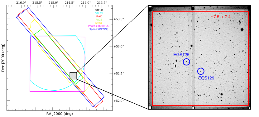
Figure 1: Spatial distribution boundaries of the UV, optical, IR, and spectroscopic redshift data used to build OTELO’s multi-wavelength catalogue (left panel). In black: the OTELO raw field, cyan: GALEX, red: IRAC, green: PACS, yellow: SPIRE, magenta: photo-z (CFHTLS), blue: spec-z (DEEP2). The right panel expands the surveyed area, showing the coadded RTF data of OTELO with its weight map (see Section 4.1 for details) overlapped in order to highlight the survey sensitivity footprint. The red polygon defines the survey’s final area (7.5′$\times$7.4′). Blue circles indicate the position of the flux calibration stars (Sec. 4.4).

Data for each wavelength was obtained from six exposures of 1100 s each, nominally dithered 18″ in a cross-shaped symmetrical pattern with a recurrence to the initial pointing, in order to fix bad pixels, residual cosmic rays and fill in the gap between detectors of the OSIRIS mosaic. This pattern also facilitates the identification of diametric ghost images (see Appendix B in Jones et al. 2002 for a succinct description of ghost families), as well as the modelling of fringes. Observations were distributed into observing blocks of two single exposures, resulting in a total of 216 RTF science mosaics. A filter, named OS 911/42 (hereafter referred as OS), centred at 911 nm and with a bandwidth of 42 nm, was used as order sorter. Figure 2 shows the Airy profile corresponding to each wavelength slice or $\lambda_{0}$, and the order-sorter transmission between Meinel bands. The RTF tuning during the observations was found to be stable at the nominal accuracy of 1 Å, as expected.

Table 1: OTELO survey: Log summary of the red tunable filter of OSIRIS (RTF) & long-slit (LS) observation campaigns. $N_{\rm obs}$ indicates the number of individual observing blocks of $\sim$1 hour each. In the case of RTF observing mode, to each block corresponds a single tuning.

Observing	Dates	$N_{\rm obs}$	Exposure	Wavelength	Mean seeing	$\sigma_{\rm seeing}$
Mode			time [ks]	range [${\rm\AA}$]	[″]	[″]
RTF	April 11  –  July 7, 2010	36	39.6	9250  –  9280	0.83	0.06
RTF	May 4  –  August 2, 2011	38	41.8	9208  –  9244	0.84	0.08
RTF	May 4  –  Aug. 10, 2013	58	63.8	9154  –  9202	0.82	0.09
RTF	March 1  –  June 5, 2014	84	92.4	9070  –  9148	0.82	0.07
LS	April 13, 2011	8	3	4800  –  9500	¡0.9	–

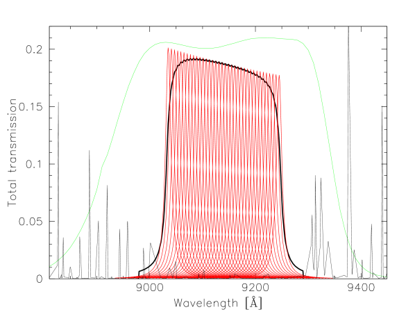
Figure 2: Characteristic transmission of the RTF for the 36 slices that define the OTELO survey spectral scan (red solid lines), as dictated by Equation 5. The thick solid line corresponds to the synthesis of OTELO RTF responses (hereafter OTELO-custom) a kind of intermediate-band ($\sim$230 Å) filter affected by the telescope, the OSIRIS camera, and the QE of the detectors. Note the location of those responses, avoiding the Meinel bands represented by the airglow spectrum (thin black line) from Hanuschik (2003). The green line represents the transmission (scaled to the total efficiency of the system) of the order sorter OS 911/42 used to acquire RTF data.

2.3 Survey products

The data reduction process described below affords astrometry-corrected and flux-calibrated images of each RTF slice. Coaddition of these images is used to obtain a deep RTF image, as well as a raw source list in a sort of photometric catalogue of RTF integrated fluxes. This catalogue is enhanced by measuring and cross-correlating ancillary information cited in Section 2.2. Individual RTF frames are also stacked to obtain representative frames of each slice, used only to obtain source cutouts for illustrative purposes.

Secondly, the OTELO survey provides a pseudo-spectrum for each object detected in the deep RTF image. Formally, a pseudo-spectrum is a wavelength convolution of the source SED by the RTF response sequence defining the scan. Unlike the spectra obtained from diffractive devices, we denoted as pseudo-spectra the vectors obtained from TF scans, properly calibrated in flux and wavelength. An example of the synthetic pseudo-spectra as provided by OTELO can be seen in Figure 3, and their further analysis is a subject of the OTELO-II paper.

The main processes and products outlined in this work, with a reference to the relevant section, are mapped in the data flow diagram of Figure 4.

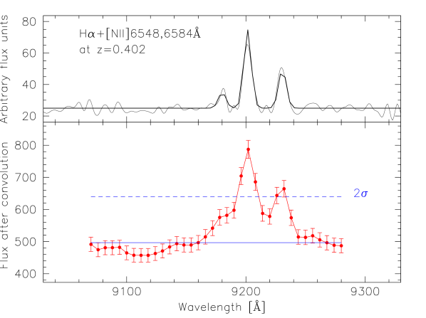
Figure 3: Example of a synthetic pseudo-spectrum as typically provided by the OTELO survey. The top panel shows a flat continuum (thick line) with H$\alpha$+[NII]$6549,6584\AA$ emission lines as Gaussian profiles (FWHM=6$\AA$). A $\log_{10}$([NII]$6584\AA$/H$\alpha$) = -0.3 ratio was chosen for this example. The observed H$\alpha$ and [NII]$6584\AA$ EWs are 15.5 and 7.7 $\AA$ respectively. Poissonian noise was added to this spectrum (thin line) and then convolved with the transmission curves represented in Figure 2 to mimic the OTELO survey scan. The result is shown in the bottom panel. Flux errors were computed by propagation, taking into account the continuum deviation at the input spectrum multiplied by the minimum pixel area, and the nominal readout noise. The dashed line represents 2$\sigma_{c}$ deviations above the fitted pseudo-continuum.

3 RTF data reduction

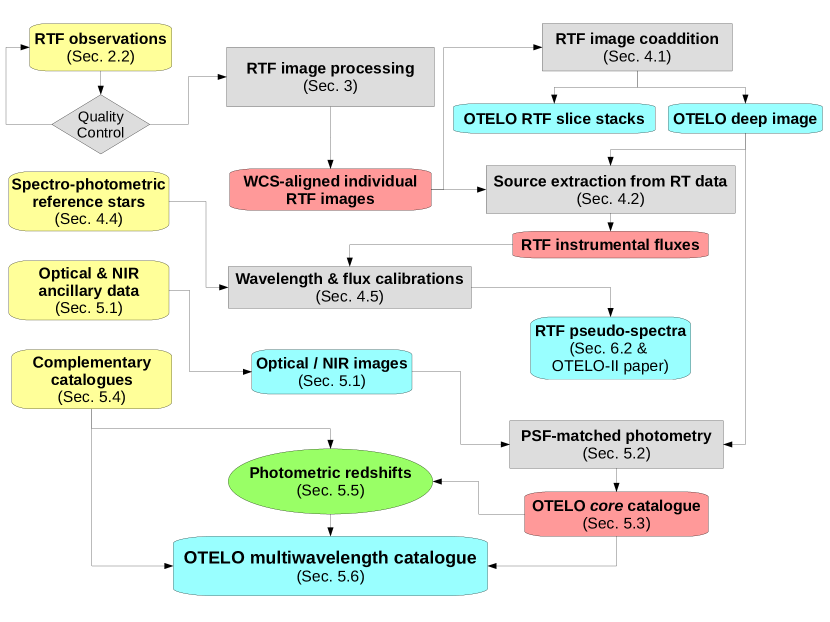
Figure 4: Data flow chart of the OTELO survey. Sharp corner grey boxes enclose processes, and the round corner ones represent input data (yellow), or intermediate (red) and final (blue) products. The green ellipse denotes both a process and a product. Where appropriate, the relevant section of this article is quoted in parentheses.

3.1 First steps

Image mosaics from the OSIRIS instrument consist of two 1049$\times$2051 pixel² frames at binning 2$\times$2 (giving a pixel scale of 0.254 ″/pixel), with a projected gap of about 38 pixel between them along the longest axis. The effect of the latter can be appreciated as the slight, vertical shadow in the middle of the right side image of Figure 1. Individual science, and all auxiliary, frames of OTELO were bias- and overscan-subtracted before trimming (according to the unvignetted FoV) using the IRAF ccdproc task. Cosmic-ray removal was carried out on each frame by means of the IRAF implementation of the stand-alone procedure lacos-im (van Dokkum, 2001), which identifies traces of these events by Laplacian filtering.

OSIRIS detectors are affected by bad pixels, mostly on the right edges and in a few columns near the upper middle part of CCD2. Bad-pixel masks for each observing epoch were obtained using a set of reduced OS night-sky flats following a standard procedure. A number of flats with low ($\sim$6000–12 000) and high counts ($\sim$33 000) were median-combined apart. The normalized ratio of such low-to-high intensity level flats was used as a bad-pixel mask. Using IRAF’s ccdmask task, we identified those pixels for which this ratio was greater than 15% and created boolean masks. Based on these masks, bad pixels in the science frames (which do not exceed 0.37% of each trimmed frame area) were finally corrected using the IRAF fixpix task, which performs an interpolation of neighbouring pixels.

Flat-fielding is not a straightforward step in conventional TF data reduction because sensitivity variations across the field radially depends on wavelength for a given tuning and, in the particular case of this survey, a non-negligible fringing component is present in all frames. In this case, pixel-to-pixel fluctuation maps in each mosaic component, observing epoch, and TF tuning were obtained from a combination of bias-reduced, defringed, and bad-pixel fixed TF dome flats. These flats were then corrected by illumination using a mode-scaled sky flat obtained with the OSIRIS order sorter OS 911/42. Low-frequency fluctuation maps were obtained from airglow emission maps representative of each slice: each bias-corrected science frame was object-masked up to 2-$\sigma$ object counts above the median background level, where $\sigma$ is the standard deviation of the local background, and each slice sextuple was median (sigma-clipped) combined. The fluctuations were measured in concentric radii, each 50 pixels around the optical centre. These measures were normalized and then used to generate a low-order surface, which constitutes an analogy to a large-scale night-sky flat. Both small- and large-scale maps were combined into a super-flat used for reducing individual mosaic components. The mean background homogeneity of science frames after applying this procedure is better than 4%.

3.2 Ring subtraction and defringing

Sky subtraction from astronomical images would formally imply control over the physical conditions of sky brightness, its gradients, the behaviour of detectors during the integration, and the optical properties of the telescope and instruments involved. This task, both impractical and intractable (Blanton et al., 2011), tends to focus on relatively simple approximations that depend on the resulting superposition of the main observational effects, and on the angular extension of the sources of interest.

As set out above, TF observations show a radial distribution of the transmitted spectral features bluewards of the central (i.e. tuned) wavelength. In practice, spectral calibration lines or airglow emission illuminating the exit pupil of the telescope appear on images as concentric rings around the projection of the TF’s optical axis. The latter are particularly strong in the NIR, as shown in panel (a) of Figure 5. Although the OTELO survey sampled a spectral region between Meinel bands, airglow OH emission bands, even with minor strengths, severely affect observations with long exposure times. As a side effect, considerable fringing usually accompanies the most intense airglow bands. Thus, an appropriate subtraction of these effects not only ensures the photometric integrity of all the sources, especially the faintest ones, but also prepares the individual science frames for a residual-free image stacking.

With these aims, we explored several technical approaches to these problems in the literature. Evidently, airglow contribution to observations can be removed on the fly from data to levels $\ll$1% by using nod-and-shuffling (Glazebrook & Bland-Hawthorn, 2001) or similar techniques (i.e. of the ON–OFF type). But the FOV reduction and/or a prohibitive increase in observing time made us discard these strategies from the very beginning of the survey, although the OSIRIS instrument was designed to be used also in these observing modes. Apart from this, there are different approaches for ring subtraction in TF images obtained in the usual mode. Jones et al. (2002) include a complete review of reasonable alternatives to remove night-sky rings. They finally lean towards a simple but effective method for those cases in which objects of interest are much smaller than the ring structure (as in the case of the OTELO survey): a background map is created by median filtering of regularly shifted (by only a few pixels) copies of the individual image to be reduced. The result is then optionally smoothed and subtracted from the original frame, leaving little or no night-sky residual, according to the authors. This procedure is a part of the TFRed collection of IRAF tasks for TF data reduction (Jones et al., 2001), identified as tringSub. It was included in the OSIRIS Offline Pipeline Software after some improvements.

Veilleux et al. (2010) model the sky background by obtaining an azimuthally averaged sky spectrum and then sweeping it around the known position of the optical axis. Prior filtering of sources and cosmic rays are performed, and constitute a part of the Maryland-Magellan TF Data Reduction Pipeline. On the other hand, Weinzirl et al. (2015) describe a technique based on an image transformation to polar coordinates with the purpose of subtracting the airglow emission, this time as straight patterns, and then applying an inverse transformation to restore image geometry.

Even though this approach is qualitatively similar to that of Veilleux et al. (2010), we do not test its performance in order to avoid flux-conserving issues in the projection/reprojection processes.

For this work, we opted to combine the advantages of the cited algorithms by performing the sky spectrum subtraction on each individual image with an automatic, two-step approach. A first cleaned image, useful only for source mapping, is obtained by subtracting a background model resulting from median-filtering eight offset ($\sim$10 pixel) copies of the input image by using the tringSub task described above. An object mask for each individual image is then constructed by flagging positive features 2-$\sigma$ above residual background using the IRAF objmask task. This initial guess for the background-subtracted image is also used to create a fringing model. Once the original image is defringed and the sources on it - traced by the object mask - are replaced by neighbouring background values, we create a series of replicas of the resulting image by rotating it around the optical centre at optimized angles. Such angles result from an equilibrium between maximum pixel sampling and the maintenance of the sky ring ellipticity ($<$0.3% in our case; J. Cepa 2017, priv. comm.) effects below a pixel in the radial direction. A median combination of these replicas before trimming to the original image size results in a sky background base image. The final background model is obtained by fitting a surface on to the base image. The procedure ends after subtraction of this model from the original image.

A complete procedure, named ringsub, was written in a single parametric IRAF script with zero user interaction and is available on request to the authors. The ringsub performance was tested and compared with tringSub and the azimuthally averaged algorithms. Science frames with large sky background fluctuations (i.e. around $\lambda_{0}=9140\AA$) were selected and catalogues created of 500 artificial stars (using the IRAF starlist task) uniformly distributed in position and brightness, according the instrumental flux range of the tested images. These stars were added to the images using the IRAF mkobject task and their fluxes recovered using the SExtractor (v. 2.19.5) application (Bertin & Arnouts, 1996) in standard mode after subtracting the sky background. Figure 5 shows a representative example of an OTELO image (CCD2) before sky subtraction with the mock stars added. Additional panels show the results of subtraction and the mean background in each case. The use of ringsub produces the smallest background residuals. If the reference-to-measured mock star flux ratio for each sky background subtraction approach is compared, it can be seen from the statistics presented in Table 2 that the ringsub algorithm yields the results nearest to the unity with the smallest dispersion. The running mean of each flux ratio as a function of the mock reference flux is represented in Figure 6. It shows that maximum departure of the ringsub ratio from unity at low flux regime is between $\sim$2 and 4%, which is in any case a fraction of the in quadrature error of the measured flux. This gives an idea of the real performance of the adopted sky subtraction routine.

Finally, as the sky-subtracted model is essentially a high-order surface fitting, the images obtained so far must be reduced by additive fringing. For each slice we median-stack the maximum number of object-masked science frames. We then arithmetically subtract this fringe model from the sky-subtracted frames with the same central wavelength.

Table 2: Mean ($\mu$), standard deviation ($\sigma$) and selected quartiles ($Q_{\rm 1,\,3}$) of the reference-to-measured ratio of all mock sources added to the example image in Figure 5, corresponding to the sky subtraction algorithms compared in this work.

Algorithm	$\mu_{\rm ratio}$	$\sigma_{\rm ratio}$	$Q_{\rm 1}$	$Q_{\rm 3}$
Azimuthally	1.011	0.077	0.999	1.028
averaged
tringSub	1.063	0.059	1.031	1.074
ringsub	1.012	0.044	1.001	1.021
(this work)

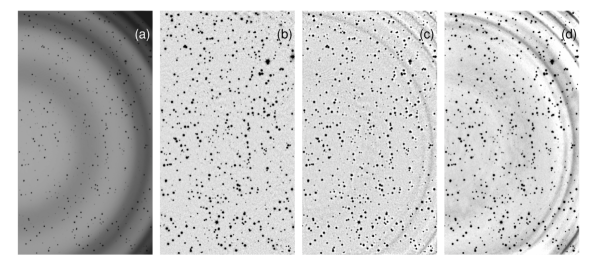
Figure 5: An example of sky-ring subtraction tests described in the text. Panel (a) shows one selected raw image of the CCD2 corresponding to a central wavelength of 9130${\rm\AA}$, with 500 artificial stars added. Arc patterns (bluer as the curvature radius grows) corresponding to equal wavelengths of the airglow band spectrum are noticeable. Panels (b), (c), and (d) show sky-ring subtracted and defringed images by using, respectively, the ringsub algorithm (adopted in this work), tringSub, and the azimuthally averaged approach. All images are scaled to the median. Below each panel is shown the mean radial spectrum (1 pixel sampling) of the original image background or residual, as appropriate.

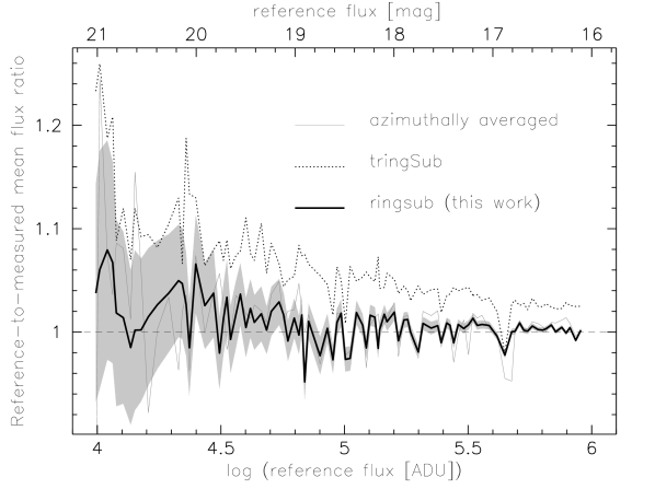
Figure 6: Running mean of the reference-to-measured flux ratio of 500 artificial stars added to an example raw RTF image before sky-ring subtraction using the ringsub procedure, the tringSub task, and the azimuthally averaged spectrum approach. Consistently with data given in Table 2, the first and last show a similar flux recovery behaviour, whilst the tringSub approach leads to a mean flux overestimation about 6%. The shaded region represents the error of measured fluxes corresponding to the ringsub routine. The error distributions of the other two procedures resemble this one. See text for details.

3.3 Astrometry

Astrometry calibration is necessary not only for referencing targets in a celestial coordinate system but also to put all the individual science images in a common spatial frame for mosaic assembly and coadding (see below) with accuracies of a few tenths of a pixel. Relative astrometry of individual science frames was referred to a custom catalogue whose construction was based on the CFHTLS Deep Field 3, 25% best seeing (D3-25), z-band data, whose internal root mean square (RMS) astrometric errors are 0.075 and 0.074 arcseconds in equatorial coordinates ($\alpha,\delta$). Concerning external errors, from a comparison with 2MASS astrometric positions, the D3-25 source catalogue used has an accuracy of 0.23″ in each coordinate. Selecting all non-saturated, point-like sources (i.e. in this case with CLASS_STAR $>$ 0.95) up to magnitude AB=23 (i.e. around the CFHTLS-provided limiting magnitude of point-like sources with a SNR$\gtrsim$10 in science exposures) from this catalogue, we consolidated a reference catalogue with 892 entries with a resulting maximal RMS internal positional error of 0.03″.

The reference catalogue was cross-matched using the IRAF ccxymatch task, with the list of sources extracted from each OTELO mosaic component. An equal number of astrometry solutions was obtained by adopting a fourth-order polynomial geometry and the non-standard TNX World Coordinate System (WCS), which has proven to be the best projection for an accurate modelling of the geometric distortion present in the OSIRIS instrument images,, which, in turn, is implemented in the IRAF ccmap task. The internal mean accuracy of the individual WCS solutions obtained (RMS residuals) is $0.043\pm 0.007$ arcseconds in the standard coordinate ($\xi,\eta$) space. Taking into account the in quadrature upper error limit of the reference catalogue, internal deviations of the WCS are below 0.068″ in both coordinates. This translates into a $\sim$0.27 pixel plate scale. WCS-based image registration for mosaic assembly and subsequent coaddition is therefore feasible within this sub-pixel regime.

Individual components of each mosaic were then warped and referenced to each other (i.e. registered) using the IRAF mscred.mscimage task, according to the corresponding high-order polynomial coefficients of the astrometric solution and conserving the instrumental flux per area unit. Before proceeding with mosaic assembly we created image weight maps, expressed in units of relative inverse variance per pixel. Weight maps influence flux error determinations and prevent false detections due to satellite trails, diffraction spikes, and certain instrumental signatures coming from detectors. Twenty of 216 RTF science frames are affected by satellite trails which were represented by zero-weight traces in those maps. Each mosaic and its resulting weight map was afterwards assembled at sub-pixel accuracy using the SWarp (v. 2.38.0) application (Bertin et al., 2002).

4 RTF data measurement

The OTELO survey is conceived as a blind, magnitude-limited spectral tomography. This involves the creation of a deep detection map, hereafter OTELO-Deep, resulting from the weighted combination of the RTF registered science frames. This image is utlized not only to maximize the detection of all real sources in the field, keeping the false-positive statistics under control, but also to be used as a source of photometric data integrated over all the slices.

4.1 Image coaddition

There are several methods of tackling the image coaddition problem. Apart from such approaches as Lucky Imaging or Fourier-based methods for combining stacks of images (Homrighausen et al., 2011), the pixelwise statistics techniques stand out among the commonly found approach of PSF homogenization (see Zackay & Ofek 2017 for a recent review of these techniques). To a first approximation, we disregard image convolution to the worst seeing before coadding because it alters the information contained in the image, degrades the PSF of almost the whole input image set, amplifies the background noise at high frequencies, creates correlated artefacts. Instead, we proceed by using a two-step coaddition scheme. First, for each slice we combined up to five of the six images dithered far enough apart (to ensure the rejection of diametric ghost images) with the best mean FWHM. Thus, nearly 83% of all RTF science frames were coadded in the corresponding slices. The remaining ones did not contribute to OTELO-Deep  but were naturally taken into account in the flux measurements described in Section 2.3. For this step we obtained the 36 image stacks by using the named clipped-mean algorithm described in Gruen et al. (2014) and implemented in SWarp. This algorithm has been specifically designed for rejecting artefacts present in individual contributors to resulting stacks. The PSF differences of selected images for each slice stack are below the canonical requirement established by its authors (i.e. $\sim$10%). The main configuration parameters adopted for SWarp runs are given in Table 3.

The results obtained were compared with the median coadding for selected slice stacks, this being the most popular artefact-free model for image coadding. As expected, the instrumental flux recovered is quite similar in both cases, but the measured SNR is 20% less in median-combined stacks than when using the clipped-mean approach. Moreover, taking into account the discrete number of individual frames for slices, median combining is not so efficient at discarding diametric ghosts and other residual artefacts of extended bright sources as the alternative used here. It is worth noting that slice stacks are useful only for producing the OTELO-Deep image and for a data cube representation of a given source.

The combination of the slice images obtained must conserve the intrinsic flux variation of the sources over the RTF scan. For this reason, and as a final step, the resulting 36 stacks were simply averaged using SWarp again to obtain the OTELO-Deep image. All coadding products include their corresponding weight maps. In particular, we used the local variance in the weight map of the OTELO-Deep image to define the highest sensitivity survey area (i.e. the region of 7.5′$\times$7.4′, or 1754$\times$1734 pixel², represented in the right panel of Figure 1). After this, and as a requirement of the source extraction procedure, all science frames (whether stacked or not) where trimmed to the same size as the OTELO-Deep image.

Table 3: Main configuration parameters in SWarp to obtain the slice representatives that contribute to OTELO-Deep image.

Parameter	Value
WEIGHT_TYPE	MAP_WEIGHT
COMBINE_TYPE	CLIPPED
RESAMPLE	Y
RESAMPLE_TYPE	LANCZOS3
SUBTRACT_BACK	N

4.2 Source extraction and instrumental fluxes from RTF data

Sources detected in OTELO-Deep were flux-measured on the image itself and on each RTF frame by using SExtractor in dual-mode. This choice conforms to the recognized performance and ease of use of this detection tool, particularly in the case of faint, extended sources (see Masias et al. 2012 for a review of source detection approaches). Under this scheme, the thresholding and final detection (segmentation) map on the OTELO-Deep is translated to each RTF image to be analysed. For this purpose, it was necessary to select the most appropriate configuration parameters for the SExtractor runs, taking into account the peculiarities of the OTELO survey. The configuration parameters adopted and which differ from default ones are given in Table 4. The main parameters are justified in what follows.

From the astrometric analysis and quality control of the OTELO-Deep image, the plate scale is fixed at 0.254 ″/pixel and SEEING_FWHM was set at 0.8″.

The detection and analysis thresholds adopted can be defined as multiples of the local background variance. High threshold values result in the missing of real fainter fluxes, but lower ones will increase the false detection rate in the final source catalogue because of correlated noise peaks in the OTELO-Deep image. This issue is discussed in Section 4.3.

As demonstrated in OTELO-II, the emission line likelihood of a source is quantified from the analysis of pseudo-spectra and the parameters derived from cross-correlation with ancillary data. The detection threshold was fixed to the maximum variance required in the OTELO-Deep background in order to recovery sources whose pseudo-spectra contain at least two adjacent slices with a flux $\gtrsim$ 2$\sigma_{c}$ above the pseudo-continuum, where $\sigma_{c}$ is defined as the standard deviation of the pseudo-continuum counts. An example of a pseudo-spectrum that dovetails this requirement (concretely, the [NII]$6584\AA$ emission line) is represented in Figure 3. The criteria that lead to the practice of this hypothesis for ELS selection are specified in Section 6.2.

The detection/analysis threshold was obtained by isolating three regions - background residual only - of 30$\times$30 pixels on the OTELO-Deep. Such cutouts were extracted from the slice images used to obtain the OTELO-Deep image to create sets of 36 stamps each. For each set we then added point-like artificial sources (as described in Section 3.2) with SNR $\simeq$ 3 on selected pairs of slice image regions, leaving intact the remaining slices of each collection. The flux of each artificial source was carefully scaled to 3$\sigma$ above the background of the selected slice cutout. This procedure was repeated six times in each collection. After this, the 36 cutouts of each collection and realization were averaged as OTELO-Deep. The detection/analysis threshold relative to the background of each averaged image was decreased in successive steps of 0.1 units until recovering the mock source flux. By linearly fitting the input SNR against the recovery thresholds, we finally obtained the detection/analysis threshold that exactly satisfies the previous hypothesis. The values found after this procedure are in agreement with the detection (= analysis) threshold adopted, for example, by Jones et al. (2002) and Galametz et al. (2013) for faint source extraction.

From this procedure, we also determined the minimum area above the threshold that a true detection should have. The SExtractor manual suggests setting from 1 to 5 pixels. We fixed it consistently at 4 pixel, which is equivalent to a circular area with radius $\sim$0.5*SEEING_FWHM.

Depending on count peaks and neighbouring fluctuations in a raw detection, SExtractor hierarchically splits the object into smaller (child) ones. The deblending threshold is set as powers of 2 (default value is 32) and constitutes the allowed number of levels in this object hierarchy, whilst the minimum flux ratio between the objects at the extremes of a decomposition is defined by DEBLEND_MINCONT. After educated tests we adopt the deblending parameters found by Annunziatella et al. (2013) from their analysis of source extraction software. In the same way we proceeded with the background estimation parameters (i.e. mesh gridding map and background smoothing factor), except that we leaned towards a local estimate of the background around a given detection rather than a global one in order to take into account the sky noise gradient on images with the radius to the optical centre. Image filtering after background fluctuations was done by means of a ‘top-hat’ function, optimized to faint, low-surface brightness source detection.

Instrumental fluxes measured in the OTELO-Deep image were directly converted into AB magnitudes. These are referred to below as OTELO_Int magnitudes. Using the effective gain and exposure time, and the estimation of the zero-point magnitude corresponding to the synthetic spectral response of the OTELO-Deep image, we obtained a MAG_ZEROPOINT of 30.504 mag.

Once the configuration parameters of SExtractor were obtained, the RTF data flow passed from the image to the catalogue domain: the standard Kron (AUTO), isophotal (ISO) and aperture (APER: 2″ and 3″ in diameter) instrumental fluxes, $F_{\rm ADU}$, of the 11237 raw sources detected on OTELO-Deep and their errors were measured in the 216 individual RTF frames, apart from position, source image geometry (including isophotal area, $A_{ISO}$), and the corresponding extraction flags. Flux measurement uncertainties were determined by means of the expression

$$\Delta F_{\rm ADU}=\sqrt{A_{\tt ISO,\ APER}\ \sigma^{2}+F_{\rm ADU}/g_{\rm\,eff}},$$ (9)

where $A_{\tt ISO,\ APER}$ are the aperture areas (isophotal or apertures respectively) in pixels, $\sigma$ is the source local background RMS, and $g_{\rm\,eff}$ is the effective gain in e^- ADU^-1, depending on the measured image (OTELO-Deep or individual RTF frame).

As described in Section 4.5, the individual instrumental fluxes must be first converted into physical units and an effective wavelength assigned to them before generating the provided pseudo-spectra.

Table 4: Main configuration parameters in SExtractor for instrumental flux measurement of RTF data using OTELO-Deep as detection image in dual mode.

Parameter	Value
DETECT_MINAREA	4 pixels
THRESH_TYPE	RELATIVE
DETECT_THRESH	0.73$\sigma$
(=ANALYSIS_THRESH)
FILTER_NAME	tophat_3.0_3x3.conv
DEBLEND_NTHRESH	64 branches
DEBLEND_MINCONT	0.001 fraction
CLEAN	Y
CLEAN_PARAM	1.0
WEIGHT_TYPE	MAP_WEIGHT
PIXEL_SCALE	0.254 ″/pixel
MAG_ZEROPOINT	30.504
BACK_TYPE	LOCAL
BACK_SIZE	64$\times$64 pixels
BACK_FILTERSIZE	8 pixels

4.3 Completeness and contamination

The completeness profile of source detections was obtained by recovering and comparing fluxes of artificial sources added to the OTELO-Deep image in a similar procedure to that described in Section 3.2. Five independent catalogues of mock sources, with a power-law distribution limited to magnitude 28 (i.e. an upper bound of the OTELO-Deep limiting magnitude or AB = 27.8: see Section 5), were randomly dropped into the OTELO-Deep image by using the IRAF mkobject task in an equal number of realizations. Mock data photometry was performed identically to the procedure described above for the observed OTELO sources. The completeness estimation is defined by the average over the five realizations of catalogued-to-recovered source number as a function of the binned OTELO_Int flux. Figure 7 shows that OTELO_Int data are complete up to $\sim$24 magnitudes and 50% completeness flux is reached at OTELO_Int= 26.38 [AB]. As is evident, this completeness estimation does not take into account the fraction of lost sources close to bright star imprints in the image, or detections that could be favoured by gravitational lenses.

As pointed out above, the nature of the so-called false-positives or false detections in a deep astronomical image is diverse. Despite having taken actions to reduce the risk of such fake objects by replacing bad pixels, adopting the clipped-mean algorithm for slice stacking, and building individual weight maps, the highest frequency and most spatially homogeneous source of false detections (FD) is constituted by the correlated noise spikes.

Using SExtractor with default parameters in OTELO-Deep and its negative image (i.e. source masked OTELO-Deep $\times$ -1), it is possible to obtain a rapid estimate of false source count statistics. This negative image is not only a fair statistical representation of the residual background of the coadded image to be measured but also retains fringing residuals, particularly the imprints of the incomplete correction of the scattered haloes from bright sources in the background subtraction or dithering holes. In our case, the asymmetry of the background model obtained from SExtractor discourages this approach. Instead of this, we created a set of images that mimic the OTELO-Deep background, which differ in the random noise pattern. Each simulation was created starting from the OTELO-Deep background model mentioned above and the corresponding background variance map, by means of a custom IRAF script. The effective gain and readout noise of OTELO-Deep, as well as the sky photon map which explain the background variance one, are the other inputs of the task. A comparison of the pixel distributions of model with each mock background image gives a mean Kolmogorov–Smirnov probability of 0.98. Such statistically identical but independent images were then measured using SExtractor with exactly the same configuration used for OTELO-Deep. All the detections were regarded as spurious and compared in number per magnitude bin with all the OTELO-Deep detections. The false detection rate (FDR) is defined as the ratio FD/(FD+TD), where TD are the true detections per bin. All FRDs obtained from each simulation were averaged (with a mean absolute deviation of 0.01) and plotted as a function of the OTELO_Int in Figure 7. The FDR provides a measure for discriminating between spurious and correlated noise, and therefore a lower bound - close to the total - of the FD in OTELO.

In summary, from the raw 10487 sources up to AB = 26.5 (i.e. the upper limit of the simulation bin that contains the 50% completeness flux of OTELO_Int), the potential FDs amount to 1150 objects. For fainter magnitudes, nearly 69% of the sources are possibly spurious. Thus, the total number of FDs is close to 1650 raw entries in the catalogue. To put it another way, in the 22 $<$ OTELO_Int$<$ 25 range, the probability that an object qualifies as spurious is about 4%. Between the latter threshold and the 50% completeness magnitude, this probability doubles every 0.5 magnitude.

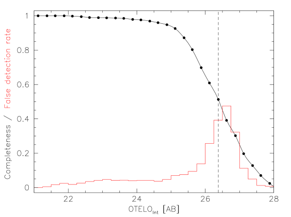
Figure 7: Detection completeness obtained from averaging the ratio of recovered-to-catalogued artificial sources in random-shoot trials on the OTELO-Deep image as described in text. A spline black curve joins averages over OTELO_Int fluxes in 0.25 magnitude bins. The dashed line at OTELO_Int=26.38 [AB] corresponds to the 50% completeness magnitude. The histogram traces the false detection rate (FDR) for the OTELO-Deep image, corresponding to an estimate of the spurious from correlated noise.

4.4 Flux calibration stars

The colour-selected F8 sub-dwarf stars in the OTELO FoV and the secondary spectro-photometric standard used to calibrate them in flux, all referred to in Section 2.2, were reduced in the standard way using IRAF.noao spectral reduction packages. All targets were observed in OSIRIS long-slit mode with a red grism at resolution $\sim$500. A slit of 1.5″ was used (with seeing conditions better than 0.9″) to achieve the maximum flux accuracy. According to $r$(AB) magnitude of the targets, total integration times were generous enough to reach an SNR$\simeq$10 between 5500 and 9500 $\AA$.

Bias frames were combined and subtracted from science spectra using the imcombine and ccdproc tasks. High-count flat-field images were combined and the result corrected by the fitting of the continuum lamp spectrum (flatcombine and response). The sky spectrum (sky flats from science images) was averaged and a sky flat was interactively fitted by a spline function using the illumination task. After correcting all science frames by illumination, wavelength calibration was carried out using transform. To this end, line identification of Ne and HgAr lamp exposures obtained with the same rotator angle as the science exposures was dumped on to a database (identify) and interactively analysed using fitcoords. Once the sky background were subtracted from individual 2D spectra, they were combined and collapsed in the spatial direction. A dereddened sensitivity curve for flux calibration was obtained from the standard star (HD126511) spectrum and the instrumental flux of the OTELO calibration stars were converted into physical ones. Figure 8 shows the reduced spectra resulting from this procedure. The mean flux error of spectra is better than 6%. The consistency of the flux density obtained with the SDSS-DR12 photometry would make it possible to apply the spectro-photometric flux calibration procedure used in the SDSS to the case of TF observations that contain such spectral-type stars in the FoV.

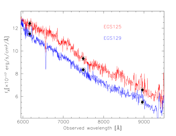
Figure 8: Spectra of the calibration stars present in the FoV of OTELO EGS pointing, as is highlighted in Figure 1. These spectra were used in turn to estimate the total efficiency of the system and its deviations depending on the particular conditions of each RTF observation. As a check on flux consistence, overlapped black dots correspond to PSF fluxes in r-, i-, and z-band from SDSS-DR12 for these stars.

4.5 Wavelength and flux calibrations

The first step in the conversion of instrumental to physical fluxes consists in deriving the total efficiency $\epsilon\equiv\epsilon\,(\lambda_{\rm ob},{\rm i},{\rm CCD})$ of the system (telescope, optics, and detector), defined as the ratio of the measured-to-reference flux $F_{\rm m}(\lambda_{\rm ob},{\rm i},{\rm CCD})/F_{\rm r}(\lambda_{\rm ob},{\rm CCD})$ using the two on-purpose calibration stars, one for each detector. As the efficiency depends on the observed wavelength, the $i$-science frame and the detector of the OSIRIS mosaic (CCD=1,2), isophotal fluxes $F_{\rm m}(\lambda_{\rm ob},{\rm i},{\rm CCD})$ were measured in each $i$-science frame, accompanied by precise wavelength determinations at the position of both stars with respect to the optical centre using Equations 7 and 8. It is necessary to emphasize that small variations in the $i$-telescope pointings and the effects of dithering on RTF observations are taken into account in the observed wavelength calculation, not only for calibration stars but for all remaining sources in the field.

The reference fluxes are measured at the observed wavelength by convolving the corresponding spectra obtained from the process described in Section 4.4 with the Airy profile approximation given by Equation 5, by setting $\lambda_{0}=\lambda_{\rm ob}$ and integrating. The measured instrumental fluxes in counts are then converted into physical ones (erg s^-1 cm^-2) for each calibration star by using:

$$F_{\rm\,m}(\lambda_{\rm ob},i)=\frac{g\,K(\lambda_{\rm ob},i)\,E_{\gamma}(\lambda_{\rm ob})}{t\,A_{\rm tel}}F_{\rm ADU}(\lambda_{\rm ob},i),$$ (10)

where $g=0.95$ e^-ADU^-1 is the CCD gain, $E_{\gamma}(\lambda_{\rm ob})$ is the energy of a photon in erg, $t$ is the exposure time in seconds, $A_{\rm tel}$ is the effective collection area of the telescope in cm², and $K(\lambda_{\rm ob})$ is the correction for atmospheric extinction, given by

$$K(\lambda_{\rm ob})=10^{0.4\,k(\lambda_{\rm ob})\,\left\langle\chi\right\rangle},$$ (11)

which depends on the extinction coefficient $k(\lambda_{\rm ob})$ and the mean airmass of the observation. In our case, we estimated $k(\lambda_{\rm ob})$ by fitting the extinction curve of La Palma in the wavelength range defined in the survey. The uncertainty in the efficiency is defined by the sum in quadrature of the errors in the measured and the reference flux (Sec. 4.4).

The total efficiency of the system (telescope + RTF + OSIRIS camera) has recently been extensively sampled, but only using the CCD2 to obtain spectro-photometric data for such calibrations. Figure 12 shows the general trend of our efficiency estimates from measurements in each individual science frame. They are in accordance with those obtained by Sánchez-Portal et al. (2015) for the H$\alpha$ imaging of a galaxy cluster at z = 0.395 using the RTF in the framework of the GLACE survey, as well as with the efficiency estimates compiled by Cabrera-Lavers et al. (2014) for the same device. A systematic differential sensitivity of a factor $\sim$1.12 between both detectors in favour of CCD2 was noted. The behaviour of our efficiencies was fitted by spline and conveniently sampled to perform the calibration at the observed wavelength of each source and RTF tuning as $\epsilon(\lambda,{\rm CCD})$.

Once the $\epsilon$-spectrum for each detector becomes available, the next step is to convert the instrumental flux of each source $s$, measured with a given CCD, to a vphysical flux density in CGS units (ergs s^-1 cm^-2 Å ^-1) by means of the expression:

$$f(\lambda_{\rm ob},CCD)_{s}=\frac{g\,K(\lambda_{\rm ob})\,E_{\gamma}(\lambda_{\rm ob})}{t\,A_{\rm tel}\,\delta\lambda\,_{\rm e}\,\epsilon(\lambda_{\rm ob},CCD)}F_{\rm ADU}(\lambda_{\rm ob},s),$$ (12)

where $\epsilon(\lambda_{\rm ob},{\rm CCD})$ is the total efficiency at $\lambda_{\rm ob}$, $\delta\lambda\,_{\rm e}$ is the effective passband width in ${\rm\AA}$ (Eq. 6), and the remaining terms are as in Equation 10. Estimation of flux error takes into account the efficiency error in quadrature, depending on the detector and the source flux measurement uncertainty as described in Section 4.2.

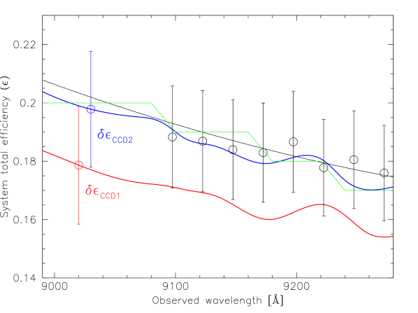
Figure 9: Spline fitting of the total efficiency of the telescope + RTF + OSIRIS camera system for CCD1 (red curve) and CCD2 (blue curve), based on the OTELO survey calibration stars and averaged for each slice. The black continuous line is the polynomial fitting from the GTC Cabrera-Lavers et al. (2014) of the values represented by the open black circles, whilst the green steped one represents the efficiency tabulated in the OSIRIS SNR Calculator. These spectra were in turn used to estimate the total efficiency of the system and its deviations depending on the particular conditions of each individual RTF observation. Overlapping black dots correspond to PSF fluxes in r-, i-, and z-band from SDSS-DR12 for these stars. The flux differences with those from SDSS are within the mean error.

4.6 RTF outputs

Two products result from the RTF data reduction: a raw set of 11 237 objects detected in the OTELO-Deep image and an equal number of calibrated pseudo-spectra. As described in Section 5, this source list is complemented with ancillary data to produce the OTELO catalogue. Even though this catalogue contains integrated fluxes expressed in different parameters (Kron, isophotal, apertures, and more sophisticated ones, as described below), we adopted the isophotal flux measured in individual RTF frames for pseudo-spectra building as the best approximation to corrected aperture flux in crowded fields. When isophotal flux pseudo-spectra of the standard stars of OTELO are compared with the convolution of their spectra, smaller deviations ($\leq$4%) than those using any other photometric parameter are revealed.

The procedure for constructing the OTELO pseudo-spectra is outlined below. For each source detected, we have a vector f_i($\lambda_{\rm ob}$) of $i=216$ effective wavelengths and physical fluxes with their errors. We should group them into $N=36$ wavelength windows or cells of $\delta\lambda\,_{\rm FWHM}/2$ = 6 Å width (i.e. the scan step) and combine the individual fluxes in each window. In practice, this is possible as long as the mean angular distance of the source to the optical centre is smaller than the size of the Jacquinot spot (i.e. a nearly monochromatic region over which the change in wavelength does not exceed by a factor $\sim\sqrt{2}$ $\delta\lambda\,_{\rm FWHM}$), or $\lesssim$1′ for the OTELO observing design.

As a consequence of the observing strategy described in Section 2.2, concerning the dithering pattern (which, in practice, also includes small telescope pointing deviations) and the wavelength change bluewards with the distance to the optical centre for a given nominal RTF tune (Eq. 7), the wavelength distribution of the vector f_i($\lambda_{\rm ob}$) not only moves bluewards as the mean distance of the source to the optical centre increases, but the f_i($\lambda_{\rm ob}$) obtained from observations could be best distributed into more than $N=36$ wavelength windows. In other words, as the source is farther from the optical centre, the f_i($\lambda_{\rm ob}$) fluxes obtained at the same central wavelength tuning could correspond to different but adjacent slices. Consequently, an OTELO pseudo-spectrum could have $N$ or slightly more data points, except for local anomalies related to the gap between detectors.

Taking these effects into account, we used a custom code to tackle the pseudo-spectra assembly. The f_i($\lambda_{\rm ob}$) vectors of each source are sorted in wavelength and, taking the first one as initial guess, the algorithm searches for accumulation points of data in $\lambda$-windows or cells in such a form that the maximum wavelength difference of a given n-tuple of data is smaller than the scan step and finds the optimal, equal-spaced wavelength sequence for each source. Each element of this sequence is a wavelength label of the resulting pseudo-spectrum. The n-fluxes associated with each wavelength are then combined using a weighted mean scheme, using the inverse square of the flux error as a weighting factor. Finally, the instrumental flux of the resulting pseudo-spectrum is converted into physical flux density units and then formatted. Figure 10 illustrates the dependence of the number of data points of a pseudo-spectrum as a function of the distance of the sources to the optical centre.

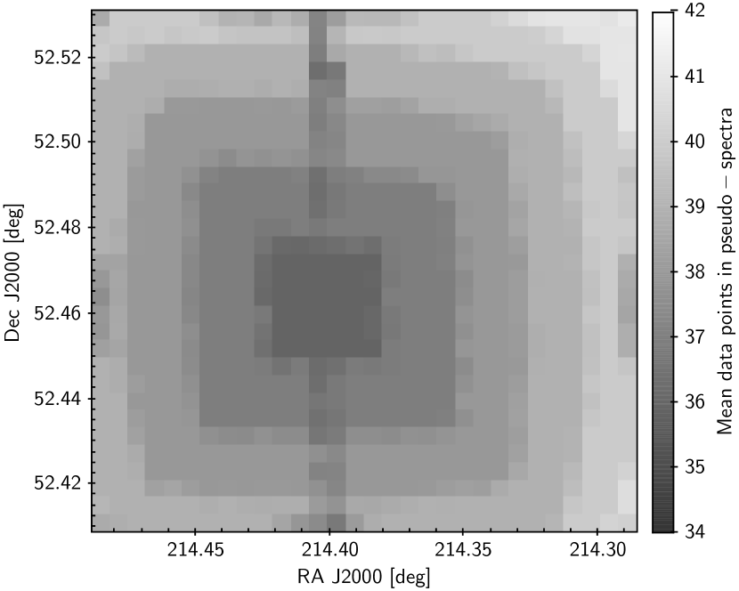
Figure 10: Spatial distribution of the mean number of data points in OTELO pseudo-spectra. The departure from concentric rings around the projected position of the RTF optical centre is an effect of the cross-shaped dithering pattern of individual RTF observations. We note that, for sources located in the vicinity of the CCD gap, the number of data points could be even smaller than the nominal number of slices: only 55 catalogued sources are affected by this contingency.

5 The OTELO catalogue

Apart from the pseudo-spectra, the main product of the OTELO survey is a raw source catalogue extracted from OTELO-Deep  suitably complemented with X-ray, UV, optical, NIR, MIR, FIR, and spectroscopic data. The process that leads to this subject is divided into two steps: we prepared a core catalogue, composed of ancillary data directly measured in images whose PSF FWHM does not exceed that of the OTELO-Deep by more that a factor $\sim$2, regardless the image scale factor, and with similar limiting fluxes. Apart from essential photometric data, the core catalogue contains identification and position coordinates of all sources measured in the OTELO-Deep image. Secondly, we cross-correlated the core catalogue with complementary data on the region surveyed to obtain the OTELO multi-wavelength catalogue. Figure 11 shows the main bands included in the latter and the respective limiting magnitudes. The following sections are devoted to explaining this process.

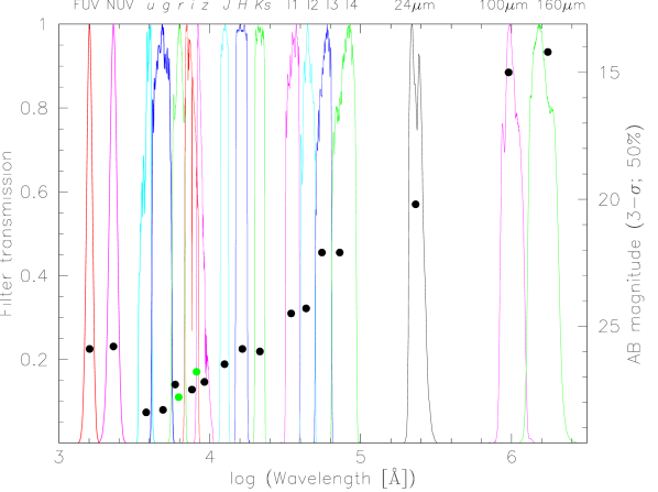
Figure 11: Bands included in the final OTELO multi-wavelength catalogue. From right to left: GALEX FUV and NUV, optical u, g, r, i, z from CFHTLS; J, H, K_s from WIRDS, I1, I2, I3, I4 corresponding to channels 1 to 4 of Spitzer/IRAC, and far-infrared 24$\,\mu$m from Spitzer/MIPS, 100$\,\mu$m & 160$\,\mu$m from PEP/Herschel. The profiles of Herschel/SPIRE are not shown. As a reference, black dots represent limiting magnitude (3$\sigma$, $\sim$50% completeness) compiled from the literature or, in the worst case, measured directly in the corresponding field data. Green dots represent the limiting magnitude of HST-ACS606 and HST-ACS814 data, whose profiles are not represented here for the sake of clarity.

5.1 Optical and NIR ancillary data

Ancillary data that meet the definition of the core catalogue are composed of optical images from the CFHTLS survey (T0007 Release), HST-ACS, and NIR data from the WIRcam Deep Survey (WIRDS, Release T0002). The CFHTLS survey data correspond to the imprint of OTELO-Deep on the Deep-3 field (1 $\times$ 1 sq.deg.; 0.186 ″/pixel), composed of 24 $u$, $g$, $r$, $i$, and $z$ stacks that reach a limiting magnitude 25 to 26 (AB; 80% completeness in extended sources). HST-ACS images in the F606W and F814W bands of the EGS were obtained as part of the GO programme 10134 (Davis et al., 2007). Data were reduced, mosaicked and pixel-resampled from native 0.03 to 0.1 ″/pixel by A. Koekemoer. The J, H, and K_s bands public data from WIRDS is a sub-section of the CFHTLS deep fields. At 50% completeness for point sources the survey reaches a limiting magnitude between 24 and 25 (AB), making it one of the deepest homogeneous surveys in the NIR to date. Further detail can be found in Bielby et al. (2012).

Native optical and NIR images and their weight maps used for this purpose were initially trimmed to the OTELO-Deep imprint plus a margin of 1′ in each dimension. A pixel homogenization to the OTELO-Deep image, conserving integrated flux per area unit, was carried out through SWarp. Using the reference catalogue and procedures mentioned in Section 3.3, we tweaked on the existing WCS calibration of each image. Image preparation concluded with their spatial registration and a final trimming of the OTELO-Deep image using IRAF wregister. After that, an accurate mean PSF of each image was fitted by using the PSFEx (v. 3.17.1) application (Bertin, 2011). Table 5 contains the main properties of the images used as input to the core catalogue. The mean PSF of the set oscillates between $\sim$0.7″ and 1″. This variation could be a critical issue when robust photometry across the bands involved is required.

Table 5: OTELO survey: Properties of the image set used to build the core catalogue. Filter profiles and limiting magnitudes are represented in Figure 11.

Survey	Filter	Filter	Filter	Limiting	Photometric	PSF
Image	Name	$\lambda_{\rm eff}$	FWHM	Magnitude	zero-point	FWHM
		[$\AA$]	[$\AA$]	[AB-mag]	[AB-mag]	[″]
OTELO-Deep	OTELO-custom	9175.0	229.4	27.8	30.504	0.87
CFHTLS	u	3881.6	574.8	30.2	30.000	1.00
CFHTLS	g	4767.0	1322.4	30.6	30.000	0.91
CFHTLS	r	6191.7	1099.1	30.3	30.000	0.86
CFHTLS	i	7467.4	1316.1	29.9	30.000	0.82
CFHTLS	z	8824.0	998.4	28.9	30.000	0.77
HST-ACS	F606W	5810.1	1776.5	29.2	26.486	0.87
HST-ACS	F814W	7985.4	1876.7	28.6	25.937	0.90
WIRDS	J	12481.5	1547.9	27.4	30.000	0.86
WIRDS	H	16158.2	2885.7	26.8	30.000	0.79
WIRDS	Ks	21337.8	3208.6	26.8	30.000	0.81

5.2 PSF-matched photometry

A number of software utilities have been developed to obtain homogeneous and reliable photometry data from multi-wavelength, combined ground- and space-based surveys with mixed bandwidths and variable PSF. Applications based on real or model source profiles (including PSF models) constitute the state of the art in these kinds of tools, among which are included for optical/NIR data ColorPRO (Coe et al., 2006), PyGFit (Mancone et al., 2013), and T-PHOT (Merlin et al., 2016). We explored different approaches to obtain reliable total fluxes and colours from the image set that contribute to the OTELO core catalogue in a quick and accurate fashion, using the OTELO-Deep image as the origin of the source detection, and with a single photometric parameter.

Inspired by the results of the analysis of the SExtractor PSF-model photometry described by Annunziatella et al. (2013) and the simulation framework to model data of the Dark Energy Survey prepared by Chang et al. (2015), we carried out our own tests to determine whether the DETMODEL parameter fulfils previous requirements within a reasonable error budget, compared with the most used ones. We built an extensive artificial source catalogue in the z-band (hereafter, $z_{\rm\,true}$) mimicking the corresponding real data for the core catalogue, as much far as the Stuff (v. 1.26.0) application (Bertin, 2009) allowed us. This condition includes identical pixel and image sizes, background noise level, effective gain, and photometric zero-point. Such a catalogue was used as input to the SkyMaker (v. 3.10.5) software (Bertin, 2009) to create three images that differ only in their PSF FWHM (i.e. 0.7″, 0.9″, and 1.1″, which cover the mean FWHM range of the real images considered here). Figure 12 shows cutouts of these simulated images. We obtained the PSF model of each z-band arbitrary image using PSFEx and then recovered the artificial source fluxes using SExtractor in dual-mode with the intermediate FWHM one as detection image.

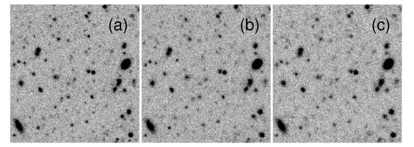
Figure 12: A detail (10′$\times$10′) of three mock images created with SkyMaker from a z-band simulated catalogue obtained using the Stuff application. Images differ only in the FWHM of their adopted PSF: (a) 0.7, (b) 0.9, and (c) 1.1 arcseconds These images were used to study the behaviour of the SExtractor application to obtain photometric parameters, including PSF-model photometry, under controlled but conditions close to those of the images used for the assembly of the OTELO core catalogue. More details in text.

Photometric error distributions from the simulated detection image (i.e. with a mean FWHM=0.9″) are pictured in Figure 13. The DETMODEL and ISOCOR parameters give a more favourable balance against AUTO, and even 3 ″ in diameter aperture (APER), photometry distributions. The error distribution corresponding to mean FWHMs of 0.7 and 1.1 arcseconds are not represented because they resemble the one plotted.

Unreliable detections (non-zero FLAGS) in any of the input catalogues were discarded. The consolidated catalogue was cross-matched in turn with the input one that contains the $z_{\rm\,true}$ photometry. Figure 14 shows magnitude difference plots of Kron (AUTO), which is the primary choice for a measurement of the total brightness, isophotal (in this case, ISOCOR), and DETMODEL parameters when compared with $z_{\rm\,true}$. These parameters were selected from a larger set, and the represented ones showed the lowest dispersion, which depends mainly on the measurement error. Attending to the overlapping running median plotted on the entire $z_{\rm\,true}$ and the dispersion profile, the DETMODEL parameter is the best choice for total flux recovery for all three mean FWHMs.

Regarding colours (Figure 15), we compared flux measured in image pairs with different mean FWHMs. The photometric parameters chosen were aperture (APER), isophotal, and DETMODEL. As in the case of Kron magnitudes for total flux parametrization, apertures (corrected) are the conventional choice to build colours, although Benítez et al. (2004) suggest that isophotal magnitudes provide the best estimate of ‘true’ galaxy colours under the same FWHM. The behaviour of DETMODEL colours is slightly better than APER colours, and the ISOCOR colours are even more consistent to zero differences but fail for faint sources. Thus, the compromise solution for single-parameter photometry in the present case is provided by SExtractor using the DETMODEL approach. Obviously, this does not preclude complementary measures with other photometric parameters.

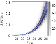
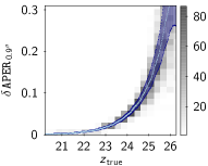
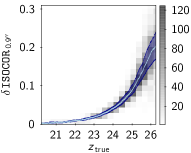
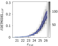
Figure 13: Distribution of photometric errors from measurements on the arbitrary z-band image with mean FWHM=0.9″for the set of photometric parameters (AUTO, APER, ISOCOR and DETMODEL) discussed in text (and also presented in Figures 14 and 15). Light blue tracks represent the running median of the distributions. Very similar trends (not shown) were also found for the two extreme mean FWHMs (0.7″ and 1.1″).

$\overline{\sf FWHM}$ = 0.7″	$\overline{\sf FWHM}$ = 0.9″	$\overline{\sf FWHM}$ = 1.1″

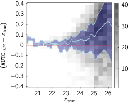
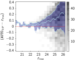
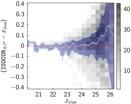
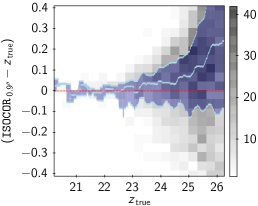
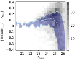
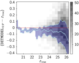
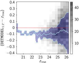
Figure 14: Distribution of measured-to-true magnitude recovered using SExtractor, from three arbitrary z-band images that only differ from the PSF FWHM (i.e. 0.7, 0.9, and 1.1 arcseconds, from left to right). Photometric parameters used (AUTO, ISOCOR, and DETMODEL) are arranged from top to bottom. Light blue tracks represent the running 25%, 50% (median), and 75% quantiles. Scale bars represent the background cells counts.

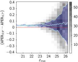
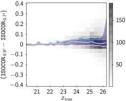
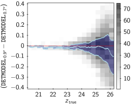
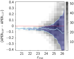
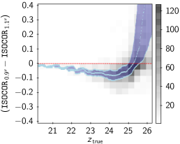
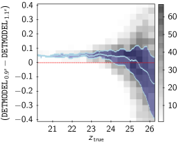
Figure 15: Distribution of measured colours recovered for paired combinations of mean FWHM. Photometric parameters used (APER, ISOCOR, and DETMODEL) are arranged from left to right. Light blue tracks represent the running 25%, 50% (median), and 75% quantiles. Scale bars represent the background cells counts.

5.3 The OTELO core catalogue

Based on the results of the simulations described above, we carried out the construction of the OTELO core catalogue by forcing DETMODEL photometry in all the images, using the OTELO-Deep image as the detection map in dual-mode with SExtractor. The catalogue contains logical and equatorial coordinates of the sources measured on the OTELO-Deep image, flux measurements in OTELO-Deep, u, g, r, i, z, J, H, K_s, HST-ACS606 and HST-ACS814 bands using the AUTO, ISOCOR, APER, and DETMODEL photometric parameters, as well as the light-spread fitting parameter SPREAD_MODEL (see Section 6.1), flux radii, peak surface brightness, isophotal area and generic flags for each source in those bands.

5.4 Complementary catalogues

The core catalogue of OTELO was cross-matched with public value-added data to obtain the final OTELO multi-wavelength catalogue. For this purpose, catalogues in X-ray, UV, mid- and far infrared were used (see Table 6).

These complementary catalogues vary in both PSF and astrometric uncertainties, the latter being the result of different treatments depending on the data source. The differences of the PSF in size and shape at the various wavelengths considered have a noticeable influence on the accuracy of the matches, namely source confusion and multiple matches. The final OTELO catalogue is the result of the cross-match of the source lists described below through an algorithm that takes into account not only the relative position of the match candidates but also their magnitude distribution and that of the background sources.

Table 6: Catalogues used for the construction of OTELO’s multi-wavelength catalogue.

Domain / Content	Survey / Mission	Spectral region	Astrometry Error	Mean PSF FWHM
			[″]	[″]
X-Rays	Chandra	0.5-10 keV	0.7	$<$0.5
Ultraviolet	GALEX	Far-UV: 1350-1780 $\AA$	0.6	4.5
		Near-UV: 1770-2730 $\AA$		5.1
Mid-Infrared	Spitzer (IRAC)	3.6, 4.5, 5.8 & 8.0$\,\mu$m	0.37	1.9, 1.8, 2.1 & 2.8
Far-Infrared (I)	Spitzer (MIPS) & Herschel (PACS)	24, 100 & 160$\,\mu$m	1.0	6.4, 7.0 & 11.2
Far-Infrared (II)	Herschel (SPIRE)	250, 300 & 500$\,\mu$m	0.5	18.2, 24.9 & 36.1
Photo-z	CFHTLS T0004 Deep-3		0.26	–
Spec-z	DEEP2 Galaxy Redshift Survey		0.50	–

In X-rays, the catalogue from Pović et al. (2009) was employed. It contains 639 X-Ray sources in the Extended Groth Strip, selected from public Chandra data in five bands: full (0.5-7 keV), soft (0.5-2 keV), hard (2-7 keV), hard2 (2-4.5 keV), and vhard (4-7 keV). When cropped to the OTELO field, 74 sources are left. The AEGIS-X catalogue (Laird et al., 2009) was also checked to include non-redundant X-ray emitters. In the OTELO field, it contains 50 sources with fluxes in four bands: full (0.5-10 keV), soft (0.5-2 keV), hard (2-10 keV), and ultra-hard (5-10 keV). Both X-ray catalogues were first cross-matched with search radii from 1 to 2.5 arcseconds. In this range, 42 sources had a match, of which more than 90% were closer than 0.5″ from their counterpart. Based on that, a new X-ray catalogue with nine bands was constructed, including those 42 sources plus the remaining 32 sources from Pović et al. (2009) and the 8 sources from Laird et al. (2009).

In the UV, data from the Galaxy Evolution Explorer (GALEX  Martin et al. 2005), as part of the AEGIS survey, were used (Bianchi et al. 2014; Morrissey et al. 2007). In total, 5185 GALEX sources fell in the OTELO field.

In the infrared, we used data from the Herschel and Spitzer Space Observatories (see Pilbratt et al. 2010 and Werner et al. 2004, respectively). We employed the first full public data release from the PACS Evolutionary Probe (PEP) survey of Herschel  which includes data in the Extended Groth Strip (Lutz et al., 2011). This catalogue uses the 24$\,\mu$m MIPS band of Spitzer as a prior to select the 100 and 160$\,\mu$m PACSbands. A total of 553 objects from this catalogue fell within OTELO’s FoV. According to Lutz et al. (2011), the astrometry precision of the catalogue is sub-arcsecond, hence we adopted a maximum position error of 1.0″ for those sources.

We also took advantage of the third data release of the Herschel Multi-tiered Extragalactic Survey (HerMES, Oliver et al. 2012), which makes use of the SPIRE instrument on board the Herschel Space Observatory. This catalogue employs the 24$\,\mu$m MIPS band as a prior to select the 250, 350, and 500$\,\mu$m bands. It contains 822 sources in OTELO’s field with an astrometrical precision of 0.5″ (Roseboom et al., 2010).

As for Spitzer, we initially employed the IRAC 3.6 $\,\mu$m-selected catalogue of the Extended Groth Strip from Barmby et al. (2008), which contains the four IRAC bands (3.6, 4.5, 5.8, and 8$\,\mu$m) and 2374 objects in our field with a precision in astrometry of 0.37″. However, this catalogue does not include the lower left corner of our field and has extremely large errors in magnitude for the faintest sources. We therefore added the catalogue made by Barro et al. (2011), which comprises 2317 sources in our field selected over the 3.6$\,\mu$m and 4.5$\,\mu$m IRAC images, measured with aperture photometry. We cross-matched these two catalogues with our own independently, and when both had a match we favoured the Barro et al. (2011) photometry.

Finally, we took advantage of two public redshift catalogues to add this information to OTELO’s multi-wavelength catalogue. One was the CFHTLS T0004 Deep3 photo-z catalogue (Coupon et al., 2009), with 7725 sources in our field obtained using optical and NIR data only. We considered a maximum positional error of 0.26″ for all the sources. The other source of redshift data was the catalogue corresponding to the 4th data release of the DEEP2 Galaxy Redshift Survey (Newman et al., 2013), which contains 517 sources in OTELO’s field. Those targets were selected from a broad-band photometric catalogue obtained with the CFHT and had absolute errors of 0.5″, as defined by the USNO-A2.0 catalogue used for the astrometry (Coil et al., 2004). The imprint of the spatial distribution of sources in each of these catalogues is shown in Figure 1.

To correlate these catalogues with our own, we used the methodology first developed by de Ruiter et al. (1977), later improved by Sutherland & Saunders (1992), which defines a likelihood-ratio ($LR$) to distinguish between true counterparts and false identifications. This approach has been successfully used to match radio and X-Ray sources to optical or infrared ones (see for example Ciliegi et al., 2003; Luo et al., 2010). Given a non-optical source, de Ruiter et al. (1977) described the $LR$ as the ratio between the probability of finding its true optical counterpart at a certain distance, and the probability of finding instead a background source at that distance. They assumed that background sources followed a Poisson distribution and only took into account the radial distance of the optical to the non-optical sources and the positional error of both.

Sutherland & Saunders (1992) later introduced magnitude information to improve the $LR$ technique. They calculated not only the probability that the true counterpart lay at a given distance from the non-optical source but also that its magnitude lay in a certain interval. In this work we have followed that approach and used the procedure developed by Pérez-Martínez (2016), defining the $LR$ as:

$$LR=\frac{q(m)f(r)}{n(m,r)},$$ (13)

$q(m)$ being the magnitude distribution of the true counterparts, $f(r)$ the probability distribution function of a true counterpart being at a distance $r$ of the object and $n(m,r)$ the surface density of background objects with magnitude $m$. For each catalogue to be matched, the procedure gets the best candidate counterpart for each OTELO source and an estimate of the reliability of the association, $R_{c}$. First, the $LR$ of each candidate is calculated as per the previous expression, keeping those with $LR$ above certain threshold. The election of this threshold is key to the final result and is obtained iteratively by maximizing the sum of the reliability and completeness of the cross-matched catalogue. The reliability $R$ of the catalogue cross-correlation is the average of the individual reliabilities $R_{\rm c}$ of each counterpart, defined as the ratio between the $LR$ of the current candidate over the sum of the others plus a completeness correction factor:

$$R_{\rm c}=\frac{LR}{\Sigma\,LR+(1-Q)},$$ (14)

where the sum is over all the candidates found for a given source, and $Q=\int_{\,-\infty}^{\,m_{\rm\,lim}}q(m)\ dm$ is the fraction of the true counterparts we are able to detect, obtained again by the iterative calculation of its magnitude distribution. The catalogue completeness, $C$, is defined as the ratio of the sum of the reliabilities of all the sources over the total number of objects in the non-optical catalogue:

$$C=\frac{\Sigma\,R_{\rm c}}{N}.$$ (15)

Depending on the density of objects in the catalogue, a safely broad radial search in a radius of 5″ was performed. From all the sources found at that distance, only those with a good $LR$ were retained after computing it for all of them with the methodology explained. In this way, we were able to select the best counterpart and calculate the reliability and the overall completeness of the result. A summary of the likelihood-ratio matching parameters and results obtained after applying this procedure is shown in Table 7.

Table 7: Results of the cross-correlation of catalogues. $LR\text{-}th$: value of the likelihood-ratio used as threshold, $R$: reliability of the matching, $C$: completeness, $N_{\rm X}$: number of sources in the non-optical catalogue and $N_{\rm matches}$: number of reliable matches found.

Catalogue	$LR\text{-}th$	$R$	$C$	$N_{\rm X}$	$N_{\rm matches}$
X-Rays	0.069	0.810	0.553	82	56
Ultraviolet	0.105	0.907	0.753	5185	4223
Mid-Infrared	0.01	0.947	0.850	2374	2128
Far-Infrared (I)	0.022	0.940	0.855	553	503
Far-Infrared (II)	0.023	0.962	0.876	822	749
Photo-z	0.281	0.901	0.568	7725	4860
Spec-z	0.542	0.992	0.886	517	461

In the cases of the Chandra and CFHTLS D3 data, the crowdedness of the latter and the sparsity of the former affect the completeness and the reliability of the results by producing more sources below the acceptance threshold $LR\text{-}th$ and higher -tuples of multiple matches with similar $LR$. In general, the reliability of the cross-match is well above 0.90, except for the X-ray case ($R=0.810$), with a mean completeness of 0.76 (median 0.85).

5.5 Photometric redshifts

The finding of photometric redshifts for OTELO sources is the first exploitation of the core plus ancillary data catalogue. Redshift estimates are mandatory for creditable labelling of the emission lines detected in OTELO pseudo-spectra and useful for a first classification of the sources based on SED fitting. In order to obtain them, we took advantage of the LePhare code (Arnouts et al. 1999; Ilbert et al. 2006), adopting the $\chi^{2}$ minimization approach to find the best fit between the observed flux of an object and different SED templates.

Three different libraries were used for the UV and optical range: one for galaxies, one for stars and one for AGN/QSOs. The galaxy library is composed of ten SED templates: 4 representative of Hubble types (E, Sbc, Scd, Im), observed by Coleman et al. (1980), and six representative of starburst galaxies, built by Kinney et al. (1996). As a survey biased to ELS finding, star-forming systems with a broad span in UV-slope ($\beta$) should be included in the OTELO distinctive galaxy template set. All these galaxy SEDs are shown in Figure 16. The AGN/QSO templates were selected from the SWIRE library, created by Polletta et al. (2007), and include templates of two Seyfert galaxies, three type-1 QSO, two type-2 QSO and three composite galaxies (starburst+AGN). As for the star library, it consisted mainly of the 131 templates calibrated by Pickles (1998), covering all the usual stellar spectral types (O-M) and luminosity classes, plus four white dwarf templates from Bohlin et al. (1995) and 26 brown dwarfs representative of stellar spectral types M, L and T from the SpeX Prism library. In order to fit the infrared (IR) part of the spectra from 5$\,\mu$m and to calculate infrared luminosities, the Chary & Elbaz (2001) library (CE01), consisting of 105 templates with different luminosities, was also used. The extinction law of Calzetti et al. (2000) was adopted, with values of extinction E($B$-$V$) ranging from 0 to 1.1 in steps of 0.1. The redshift range was defined from 0.04 to 10, in intervals of 0.05.

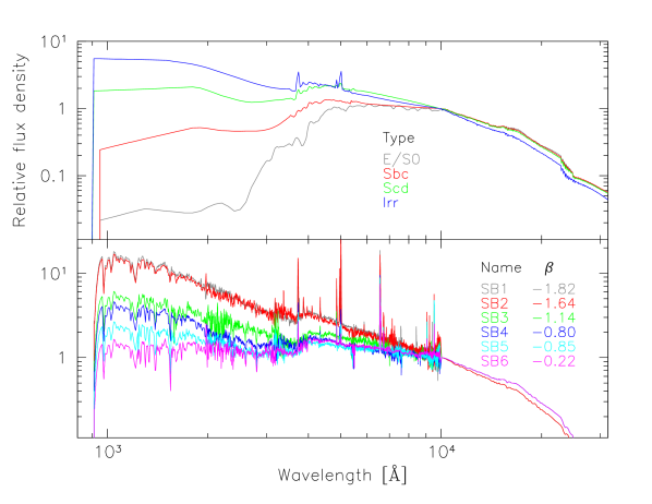
Figure 16: Galaxy templates used in photometric redshift estimations. Upper panel show the basic set of Hubble types E/S0, Sbc, Scd, and Irr from Coleman et al. (1980), whilst the lower panel contains the collection of star-forming galaxy templates from the Kinney et al. (1996) Atlas. Their measured UV slopes, $\beta$ (2200-3100 $\AA$), are also given. In both cases the continuum was extrapolated in UV and IR as explained in Arnouts et al. (1999).

In summary, for each problem source LePhare provides photometric redshift solutions for each template set in the UV and optical range. Apart from redshift, the solution includes the best fitted template and the $\chi^{2}$-statistic. Each LePhare launch starts with the creation of the filter library, which includes, in our case, all the filters described in section 5: FUV and NUV from GALEX, u, g, r, i, and z from CFHTLS, J, H, and K_s from WIRDS, the four IRAC bands, 24$\,\mu$m from MIPS, 100 and 160$\,\mu$m from PACS, and finally 250, 350 and 500$\,\mu$m from SPIRE, and -optionally, as explained below- the OTELO_Int data. Apart from redundancy with the i and z bands of CFHTLS, resampled data in HST-ACS606 and HST-ACS814 do not cover the entire OTELO FoV and were excluded from photo-z estimates. Given this set of filters, magnitudes (AB) are then computed for each template in the UV and optical range sets described above at each value of redshift and extinction in the corresponding input grids. A distribution of $\chi^{2}$ estimates is obtained from a comparison of the observed and the model magnitudes for each one of the ten galaxy templates in order to find the best redshift solution. If an additional local minimum in the $\chi^{2}$ distribution is significant, a secondary redshift solution and its corresponding template fit is also provided. The execution of the code continues with the replication of this procedure but using the AGN and star template sets. This analysis is independent of the previous step and skips the finding of secondary solutions. For AGN templates an additional redshift solution is given. For stars the expected $\chi^{2}$-statistic is provided. Finally, if the problem source have observed IR data, LePhare fits a CE01 template in the flux dimension adopting the main photometric redshift solution previously found. Table 8 contains an extensive list of the photometric redshift parameters given in the OTELO multi-wavelength catalogue.

In order to maximize the analysis possibilities and the choice of a z${}_{\rm\,reliable}$ for each suitable OTELO source, the code was launched twice: once for both the core plus ancillary data catalogue – i.e. including the OTELO_Int data – and again using only the broad-band data, as is traditionally done. In the first case, the contribution of emission lines was taken into account when computing the template magnitudes. To that end, an extra filter was added to the filter library (see Figure 2), corresponding to the spectral responses of the tunable filters and representing the spectral window of OTELO_Int, when data from the latter are included.

Both solution sets, including either the OTELO_Int flux in the redshift estimate or not, are given in the multi-wavelength catalogue described in Section 5.6. Unless otherwise mentioned, in the remainder of this article we refer to the photometric redshift as that obtained using all the core plus ancillary data. Examples of the photometric redshift fits using LePhare for ELS candidates at different redshifts are shown in Figure 17.

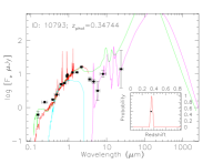
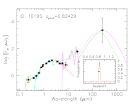
Figure 17: Examples of SED fitting performed by LePhare in order to obtain photometric redshifts. From left to right, OTELO sources with ID 10793, 10195, and 7431 at z$\sim$0.35, 0.82 and 1.46, respectively, are shown. Black dots are the observed fluxes of the source (including (OTELO_Int data), and their errors are given by vertical bars. Horizontal bars represent the filter widths. The red curve represent the best-fitting galaxy template from which the primary solution of the photometric redshift is obtained. The blue spectrum represent the stellar template that best fits the observed SED, while the pink one corresponds to the best fit of the Chary & Elbaz (2001) templates of the infrared part of the SED (when applicable) for the photometric redshift obtained. The spectrum in green is the best alternative (QSO) photo-z solution using Polletta et al. (2007) templates.

To calibrate the accuracy of the computed best-fitted photo-z, we compared them to the spectroscopic redshifts up to z $\sim 1.5$ from the DEEP2 catalogue (Fig. 18), described in section 5.4, which are flagged as secure/very secure redshifts. A total of 368 OTELO sources match with DEEP2 data entries. The best fit for 17 of these sources corresponds to QSOs/AGN instead of galaxy templates. Then, assuming that the true redshift, z${}_{\rm\,real}$ = z${}_{\rm\,DEEP2}$, we found that the redshift accuracy —$\Delta$z—/(1+z${}_{\rm\,DEEP2}$) is better than 0.2 (0.1) for 96% (87%) of all selected sources with spectroscopic redshift (see Fig. 19). Nearly identical results are reached if photo-z solutions are estimated without data from OTELO-Deep. As noted from this figure, there does not seem to be a dependence of accuracy scatter on the apparent magnitude of the source.

Figure 18: Plots of z${}_{\rm\,phot}$ as a function of z${}_{\rm\,DEEP2}$. Dashed lines indicate —$\Delta$z—/(1+z${}_{\rm\,DEEP2}$) = 0.2. Encircled dots correspond to multiple, unresolved sources, or objects with images on the border of OTELO-Deep. See text for further details.

Figure 19: Plot of $\Delta$z/(1+z${}_{\rm\,DEEP2}$) versus OTELO_Int (left panel) and the distribution of the former (right). Dashed lines and encircled points have the same meaning as Figure 18.

We checked one by one all 13 fof the 368 sources that appear outside of the region defined by —$\Delta$z—/(1+z${}_{\rm\,DEEP2}$) $<$ 0.2 in Figures 18 and 19. This examination went through the analysis of the SED fit quality, as well as the corresponding pseudo-spectra and source cutouts from HST-ACS606 and HST-ACS814 imaging data at native spatial resolution. Such images show evidence of multiple components, unresolved in ground-based data, for seven out of 13 objects. It is likely that the composed, uneven SED of these sources are poorly represented by photo-z solutions based on the selected templates. On the other hand, two of these outliers correspond to sources directly located on the border of the OTELO FoV. Outliers belonging to these categories are shown encircled in the mentioned figures, and all but two of them have unusually large $\chi^{2}$ values ($>10^{3}$) from galaxy template fitting when the median of its distribution is 10.62.

Despite the fraction of inaccurate SED fits ($\sim$4%), the level of accuracy achieved, if extrapolated to all the sources with a fair $\chi^{2}$-statistic, is good enough to meet the primary goal of the redshift estimates; that is, to obtain a z${}_{\rm\,reliable}$ that serves to guide the emission-line identification in otelo pseudo-spectra. Photo-z distribution of preliminary ELS candidates are given in Section 6.2.

5.6 Data integration and the multi-wavelength catalogue

Matched core (Section 5.3) and complementary (Section 5.4) catalogues were integrated with the results of the photometric redshift analysis described above, yielding the OTELO multi-wavelength catalogue, whose entries are listed in Table 8. The catalogue includes solutions with (z_BEST_deepY) and without (z_BEST_deepN) photometry measured on the OTELO-Deep image, together with secondary solutions if found. As described in Section 5.5, the catalogue also contains redshift solutions of QSO/AGN models. For objects with detected FIR emission, total IR luminosity is given. Photo-z data for each template set include in addition the best model fitted and the $\chi^{2}$-statistic. Spectroscopic redshifts (zspec) from DEEP2 survey (Newman et al., 2013) with a quality flag ${\rm Q}\geqslant 3$ were also incorporated.

Table 8: Contents of the OTELO multi-wavelength catalogue.

Parameter	Description
idobj	OTELO object number in raw catalogue
x, y	Logical coordinates of the object in OTELO-Deep image
ra, dec	Equatorial coordinates (J2000.0) of the object in OTELO-Deep image
dmodelX	Magnitude from detection model-fitting in X-band of the core catalogue
edmodelX	RMS error on detection model-fitting magnitude
isoareaX	Isophotal area
fradiX-n	source radius at n-per cent of flux, with n=20, 50, 80
spreadmX	Spread parameter from model-fitting magnitude
espreadmX	Spread parameter error from model-fitting magnitude
clasX	SExtractor star/galaxy classifier output
iflagX	SExtractor standard flag
totalZ	Total magnitude in the Z-complementary catalogue
etotalZ	Total magnitude error in the Z-complementary catalogue
els_preliminary	ELS preliminary candidate flag
zspec	Spectroscopic redshift from DEEP2 survey (Newman et al., 2013)
zp_reliable_T04	Most reliable photo-z from CFHTLS-T04 (Coupon et al., 2009)
zp_first_T04	Best photo-z estimate from CFHTLS-T04
zp_left_68_T04	Minimum photo-z from $\Delta\chi^{2}$ = 1.0 (68%) from CFHTLS-T04
zp_right_68_T04	Maximum photo-z from $\Delta\chi^{2}$ = 1.0 (68%) from CFHTLS-T04
z_BEST_deepQ	Best galaxy model photo-z estimate
z_BEST68_LOW_deepQ	Minimum photo-z from $\Delta\chi^{2}$ = 1.0 (68%)
z_BEST68_HIGH_deepQ	Maximum photo-z from $\Delta\chi^{2}$ = 1.0 (68%)
CHI_BEST_deepQ	Lowest $\chi^{2}$ for galaxy templates
MOD_BEST_deepQ	Galaxy model for best CHI_BEST
EBV_BEST_deepQ	Reddening colour excess E($B$-$V$)
NBAND_USED_deepQ	Number of bands used in photo-z fitting
z_SEC_deepQ	Secondary photo-z solution
CHI_SEC_deepQ	$\chi^{2}$ for secondary photo-z solution
MOD_SEC_deepQ	Galaxy model for CHI_SEC
z_QSO_deepQ	QSO model photo-z
CHI_QSO_deepQ	$\chi^{2}$ for Z_QSO
MOD_QSO_deepQ	Galaxy model for CHI_QSO
CHI_STAR_deepQ	$\chi^{2}$ for MOD_STAR
MOD_STAR_deepQ	Fitted star model
LUM_TIR_BEST_deepQ	IR luminosity from MOD_FIR (when apply)
LIB_FIR_deepQ	FIR library used (when apply)
MOD_FIR_deepQ	FIR model fitted (when apply)
CHI_FIR_deepQ	$\chi^{2}$ for FIR template fitting (when apply)

Following Coupon et al. (2009), we can define an estimate of the photo-z uncertainty $\delta\,$z${}_{\rm\,phot}$ by

$$\delta\,({\scalebox{0.9}{\tt z\_BEST\_deepQ}})=$$ (16)

$$\lvert{\scalebox{0.9}{\tt z\_BEST\_LOW\_deepQ}}-{\scalebox{0.9}{\tt z\_BEST\_HIGH\_deepQ}}\rvert/2,$$

where ${\tt z\_BEST\_[LOW,HIGH]\_deepQ}$ are the low and high redshift values included in the OTELO multi-wavelength catalogue, corresponding to the 68% confidence interval of the photo-z probability distribution function (PDF) obtained with LePhare, and Q = Y,N, depending whether or not the OTELO_Int data are included in photo-z solutions, respectively. Thus, based on the photo-z accuracy given above, a useful criterion to discard possible photo-z outliers could be defined by

$$\delta\,({\scalebox{0.9}{\tt z\_BEST\_deepQ}})\leqslant 0.2\ (1+{\scalebox{0.9}{\tt z\_BEST\_deepQ}}).$$ (17)

Thus, if we choose z${}_{\rm\,phot}$ = z_BEST_deepY, from the 9709 sources with non-null photo-z solutions, a total of 6600 have an uncertainty $\delta\,$z${}_{\rm\,phot}$ $<$ 0.2 (1+z${}_{\rm\,phot}$). This constraint is used in what follows, for example, to debug preliminary ELS selections.

5.7 OTELO public data release

From extensive data described in previous sections, the OTELO Team has selected the following value-added data for the first public data release:

• A basic catalogue containing (i) the identification of the source, (ii) equatorial coordinates, (iii) the optical and NIR photometric data from the core catalogue (Section 5.3), (iv) the best photometric redshift solutions and uncertainties (Section 5.6), and (v) a morphology classification flag (Nadolny et al. 2019; in prep.).

• A supplementary catalogue containing (i) the identification of the source, (ii) the X-ray, UV, MIR and FIR photometric data and additional redshift data (i.e. CFHTLS and DEEP2), all obtained from complementary catalogues as described in Section 5.4.

• A public version of the Web-based GUI described in OTELO-II, containing (i) the identification data of the source, (ii) a set of 8″$\times\,$8″ image cutouts of the source from ground-based and HST imaging data available, (iii) all the photometric redshift solutions included in Table 8 and their corresponding SED (as represented in Figure 17, and (iv) the pseudo-spectrum of the source.

Both catalogues and the Web-based visualisation tool, along with the corresponding Explanatory Supplement, will be publicly available from the OTELO survey URL (see Section 1) from the second half of 2019.

6 OTELO demographics

6.1 Star–galaxy separation

The OTELO survey could be used as a true sensitive probe of Galactic thick disk and halo structures (Alfaro et al., 2003). A reliable segregation of stars present in the OTELO field is not only interesting in itself because of the existence of e.g. potential cool and ultra-cool sources, but also for the analysis purposes that follow in the next sections of this work. To this aim, the standard approach takes advantage of a combination of the source image geometry and optical/NIR colour criteria.

Apart from the usual CLASS_STAR star/galaxy separator of SExtractor, we also obtained the SPREAD_MODEL classifier for each band, which is a by-product of the PSF-model photometry that quantifies the differences between PSF-like and resolved objects through a linear discriminant (Desai et al., 2012). In a comparison of different methods used for star/galaxy separation, Annunziatella et al. (2013) concluded that the SPREAD_MODEL largely improves the classification of extended and point-like sources down to such faint apparent brightness as $B$=26 for stellar ones, above the performance of the CLASS_STAR parameter or software applications such as DAOPHOT and ALLSTAR.

Figure 20 shows the distribution of the SPREAD_MODEL compared with the CLASS_STAR parameter for the OTELO sources detected in z-band. Even though any photometric band can be used for this task, the choice of the z-band utilizes data that show the smallest mean PSF FWHM (see Table 5). As expected, from this plot it is clear that SPREAD_MODEL gives a sharp sequence of stellar-like sources around zero, and that extended sources display increasingly positive values. Remarkably, the vast majority of sources that could have been selected as point-like using the CLASS_STAR $\geqslant$ 0.95 criterion are clearly deviate from the star-like sequence up to AB$\sim$24. At this value both sequences begin to merge. On this basis, we adopted AB=24.5 z-band magnitude as a flux limit for star/galaxy separation and a SPREAD_MODEL parameter threshold below zero to obtain a collection of 197 point sources.

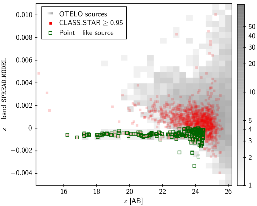
Figure 20: Example in the z-band of the SPREAD_MODEL performance in the star–galaxy separation. Red squares represent sources with CLASS_STAR $\geq$ 0.95. Point sources selected (open squares) are brighter than AB=24.5 z-band magnitude and limited by a SPREAD_MODEL value below which the star-like sequence is clear.

As mentioned in Section 5.5, an extensive set of AGN and stellar templates was used during LePhare runs to obtain best SED fits of all OTELO sources, independently of the main photo-z solution obtained through galaxy templates. Following Yang et al. (2014), we used the $\chi^{2}_{star}<\chi^{2}_{galaxy}$ as a valid criterion to depurate the star selection based on the SPREAD_MODEL. The 81 point-like sources that met this condition are represented in Figure 21 and constitute a fair sample of Galactic source candidates subject to possible spectroscopic follow-up. More than 90% of these sources have colours congruent with those of a sequence of Galactic halo stars obtained from models of Allende Prieto et al. (2014). A similar fraction of the star candidates are located in the expected region of the BzK-equivalent diagram presented in Section 6.3.

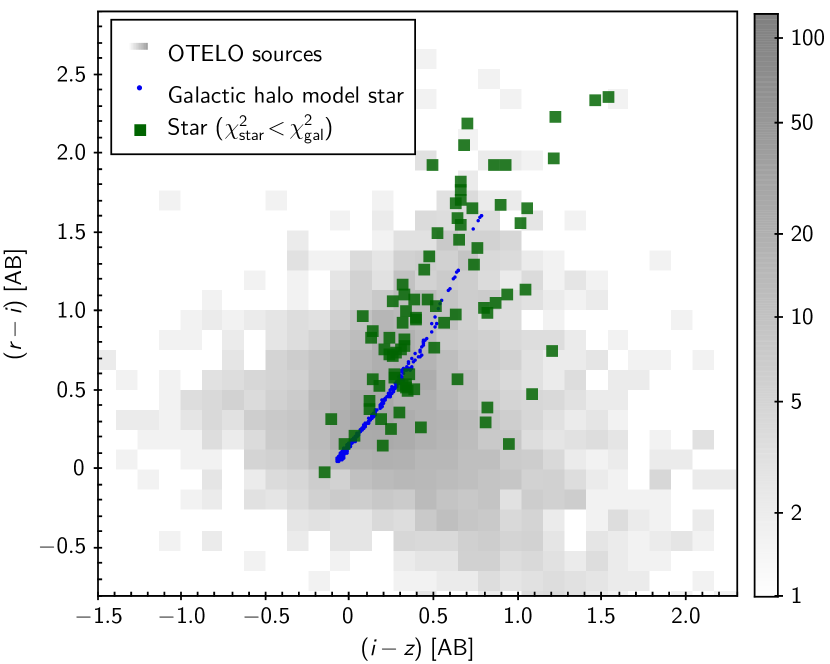
Figure 21: ($r-i$) versus ($i-z$) colours distribution of the final OTELO catalogue. Green squares represent sources classified as stars and the blue dots trace a sequence of typical Galactic halo stars from Allende Prieto et al. (2014). See text for details.

The best templates fitted to the star candidates are mainly distributed between spectral types K and M (14 and 46 sources, respectively), of which 45 correspond to sub-dwarfs. Most of the templates fitted belong to the Pickles Atlas (Pickles, 1998), and five of the M-type stars were well-fitted by SpeX Prism templates.

A catalogue simulation run of the Besançon model of the Galaxy (Robin et al., 2003), without kinematics, predicts for the OTELO field a total of 112 stars between magnitudes 16.0 and 24.5 (z-band of CFHTLS) in a solid angle of 0.014 deg² around l=96^∘.46 and b=60^∘.03. According to this, the expected stars on the OTELO field would be distributed between spectral types F3 and M7, with a luminosity class corresponding to dwarfs or sub-dwarfs, except two that would belong to the red sub-giants. A detailed study of the OTELO Galactic component with new statistical estimates is a part of a forthcoming contribution.

6.2 Preliminary ELS selection

According to the science goals of OTELO, once obtained the calibrated pseudo-spectra corresponding to each entry of the multi-wavelength catalogue, it is necessary to select the ELS candidates. The creation of robust lists of ELS segregated by emission line(s) necessarily involves a sequence of procedures, from which the first two are described in this paper. The completion of these tasks contributes towards quantifying the potential and intrinsic merits of the survey. Further analysis of the preliminary ELS selection is a part of the scope of OTELO-II.

Preliminary ELS selection starts with blind processing of the individual pseudo-spectra. A straightforward application reads each calibrated pseudo-spectrum, determines a constant pseudo-continuum flux density ($f_{\rm c}$) and then estimates median absolute deviation ($\sigma_{\rm MAD}$) of the flux vector (f[i], i=1 to N, and N = number of the RTF scan slices). This is a more robust measure of the pseudo-continuum fluctuations than the simple standard deviation when deal with data with strong fluctuations (i.e. the absorption/emission features in a pseudo-spectrum). Assuming that the fluctuations of the pseudo-continuum are normally distributed, $\sigma_{\rm MAD}$ can be simply converted to standard deviations $\sigma_{\rm c}$ around the median multiplying by a factor that depends on the quantile function, $\Phi^{-1}$.

An emission/absorption feature in a given pseudo-spectrum is considered noticeable if (i) at least two consecutive slices of the pseudo-spectrum are above/below a value defined by $f_{\rm c}$ +/- 2 $\times$ $\sigma_{\rm c}$, or (ii) only one slice flux is above/below this value, but with an adjacent point above/below $f_{\rm c}$ +/- $\sigma_{\rm c}$ and the other above/below $f_{\rm c}$. An example of the former is the [NII]$6584\AA$ emission line in the synthetic pseudo-spectrum represented in Figure 3.

Both criteria are complementary and not mutually exclusive (i.e. they are partially correlated). Together, they are consistent with the condition behind the source detection threshold in the OTELO-Deep image (Section 4.2). If the noise around the pseudo-continuum approximates the Gaussian distribution, the independent probabilities that any feature in a given pseudo-spectrum with N $\geq$ 36 data points satisfies criteria (i) or (ii) because it is a random event are, respectively, 0.018 and 0.051. Therefore, the joint probability of having false-positive emission/absorption line allocation in a pseudo-spectrum is at most $\sim$6%.

Using these criteria, an upper bound of the observed equivalent width (EW${}^{+}_{\rm obs}$) in emission/absorption is measured in each pseudo-spectrum by integrating all the flux contributions above/below the pseudo-continuum. All sources of OTELO survey in the EW${}^{+}_{\rm obs}$ vs. $f_{\rm c}$ space are represented in Figure 22. A total of 5322 from 11237 sources met one or both selection criteria in terms of emission feature. This subset constitutes the preliminary ELS candidates selected from pseudo-spectra. These sources are highlighted in Figure 22.

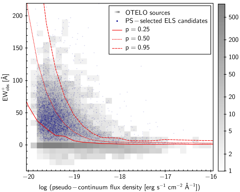
Figure 22: Upper-bound of observed equivalent width (EW${}^{+}_{\rm obs}$) as a function of the flux density of the pseudo-continuum measured on the OTELO pseudo-spectra (PS). The preliminary ELS candidates, selected as described in the text, are pictured as blue dots. The red lines represent the minimal EW${}^{+}_{\rm obs}$ at p=0.25, p=0.50 and 0.95, obtained from RTF data simulations described in OTELO-II. In this figure (and hereafter) the background grid represents the binned sum of all OTELO sources in the space of the variables represented.

Assuming a Gaussian profile, the width of an emission line in a pseudo-spectrum of OTELO can be written as the sum in quadrature of line intrinsic and instrumental widths, the latter being given by Eq. 6 for OTELO RTF data, which is close to 19.4 Å. This condition is a good approximation as long as the line intrinsic width $\ga\delta\lambda\,_{\rm FWHM}/2$ = 6 Å (Section 2.2).

When the observed width of a given emission line reaches $\sim$50 Å, that is $\sim$25% of the OTELO spectral range (i.e. $\sim$230 Å or the FWHM of the OTELO-custom filter), the convolved line begins to saturate the pseudo-spectrum, resulting in an overestimate of the pseudo-continuum. Under these circumstances, a likely ELS candidate is automatically ruled out if only the information given by the pseudo-spectrum is regarded. For instance, the width of AGN broad lines span from $\Delta v_{\rm FWHM}\sim$500 km s^-1 (a little more than the upper limit of the narrow line component) to $\ga 10^{4}$ km s^-1, with typical values of $\sim$5000 km s^-1 (Peterson, 1997). This translates into 25 Å $<$ FWHM $\la$ 300 Å (RTF-convolved) at the central wavelength of the OTELO scan. In addition, RTF data simulations using synthetic pseudo-spectra (Ramón-Pérez, 2017, OTELO-II) support these effects, and confirm that potential ELS with intrinsic line widths above FWHM $\sim$60 Å can be lost if an alternative recovery method is not enforced. OTELO data can be used to complement the ELS selection from pseudo-spectra by adopting the colour-excess technique traditionally used in narrow-band surveys.

There are several approaches to the colour selection of ELS (Pascual et al., 2007). The particular case developed below corresponds to the scheme of using an intermediate-band filter (OTELO-custom) to measure the line+continuum flux (OTELO_Int), inside a broader one for continuum sampling (z-band). The complementary search for ELS is then performed by selecting (z-OTELO_Int) colour excess with respect to a zero point and above its uncertainties, as a function of the OTELO_Int. Comparing this colour around zero value (i.e. —(z-OTELO_Int)— $<$ 0.5; 4337 sources) with the corresponding flux excess in OTELO pseudo-spectra, parametrized by the EW${}^{+}_{\rm obs}$, we found that the zero-point of the (z-OTELO_Int) colour diagram does not have offsets above 0.008 mag, with a near zero dependence on the EW${}^{+}_{\rm obs}$. Therefore, the (z-OTELO_Int) zero calibration is accurate enough to be used for ELS extraction.

Following Bunker et al. (1995), isolines of colour-excess significance were computed using

$$(${z}-{OTELO${}_{\rm Int}$}$)=-2.5\log_{10}\ \left[1-\delta\ \Sigma\ 10^{-0.4\ (zp-{\scalebox{0.7}{{OTELO${}_{\rm Int}$}}})}\right],$$ (18)

where $zp$ = 30.504 is the photometric zero-point of OTELO_Int data, $\delta$ is the sum in quadrature of the sky background in each band, and $\Sigma$ the colour excess significance. In this case, additional cuts or limits in colour (or equivalently observed EW) were disregarded.

All sources with $\Sigma>2$ and a signal-to-noise ratio on the continuum better than 5$\sigma$ were selected, yielding a total of 3226 ELS candidates. From these sources, 1542 (48%) were already selected by emission excess in pseudo-spectra as described above. Figure 23 shows the constraints described besides the remaining 1684 colour-selected only ELS candidates.

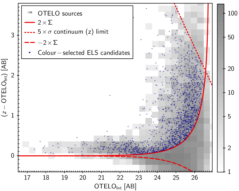
Figure 23: A (z-OTELO_Int) colour-magnitude diagram used for a selection of ELS complementary to the preliminary one based on pseudo-spectra. The candidates are represented by blue dots. This selection is bounded by a 2-$\Sigma$ isoline of colour significance, and a 5-$\Sigma$ limit in z (dotted line). All fluxes correspond to the DETMODEL measurements. OTELO_Int flux is measured on the OTELO-Deep image.

If, therefore, the ELS candidate set that meets the selection criteria applied to pseudo-spectra is joined with the colour-selected ELS one without redundancies, a total of 7006 preliminary line emitters is obtained. Regardless of the selection criterion used, all ELS candidates in the OTELO multi-wavelength catalogue are identified with the corresponding flag, els_preliminary (see Table 8).

The sky footprint and spectral range of the OTELO survey define comoving volumes corresponding to noticeable emission lines. In order to segregate those preliminary ELS candidates by chemical species and go one step further in refining the number statistics of line emitters, it is necessary to cross-correlate the selection described above with photometric redshift data. Accordingly, from the 7k+ set of preliminary ELS, a total of 4336 sources satisfy the photo-z constraint in Equation 17. The frequency of best galaxy template fitting for these ELS candidates is shown in Figure 24. The best fits for most than a half (55%) of ELS correspond to the two hardest UV-slope starburst templates.

Figure 24: Primary z${}_{\rm\,phot}$ template distribution the preliminary ELS candidates of OTELO, as described in Section 6.2. Names of templates are the same as in Figure 16. The templates with the highest UV-slope (SB1 & SB2) are the best fits for more than 55% of the ELS candidates that fulfil the condition in Equation 17.

The photo-z distribution of these sources up to redshift z=4 is provided by the histogram of Figure 25, whose main spikes are associated to the bright emission lines scanned below this redshift. A total of 1516 candidates can be directly attributable to such spectral features, and a raw census of them is given in Table 9, along with the redshift ranges and comoving volumes explored.

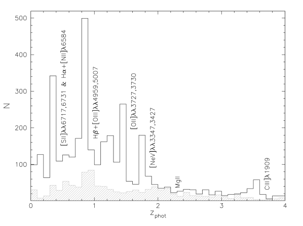
Figure 25: Distribution of photometric redshifts up to z=4 obtained with LePhare for the preliminary ELS candidates of OTELO, as described in Section 6.2. As a comparison, the grey filled histogram corresponds to the photo-z of HDFN galaxies (Fernández-Soto et al., 1999) under similar conditions to ours. The remarkable excess in the histogram is labelled on the right side with the name of the corresponding redshifted emission lines.

Regarding the high redshift (z $>$ 4) regime, a total of 611 from the 4336 ELS with acceptable uncertainty $\delta({\tt z\_BEST\_deepQ})$ are catalogued, and 296 of them are preliminary ELS candidates for the species listed in Table 10.

Table 9: Counts of preliminary ELS candidates with acceptable uncertainty and photo-z $\lesssim$ 4.

Emission line(s)	Redshift range	Comoving volume [Mpc3]	Raw ELS counts
[SII]$\lambda$6717,6731	0.33-0.38	1.769 $\times\ 10^{3}$	254
H$\alpha$ + [NII]$\lambda$6548,6583	0.36-0.42	2.463 $\times\ 10^{3}$	129
[OIII]$\lambda$4959,5007	0.79-0.87	8.958 $\times\ 10^{3}$	416
H$\beta$	0.85-0.91	7.134 $\times\ 10^{3}$	186
[OII]$\lambda$3726,3729	1.41-1.49	1.388 $\times\ 10^{4}$	261
[NeV]$\lambda$3426	1.63-1.78	2.787 $\times\ 10^{4}$	209
MgII	2.21-2.32	1.995 $\times\ 10^{4}$	26
CIII]$\lambda$1908	3.60-3.87	4.914 $\times\ 10^{4}$	35

Table 10: Counts of high-z preliminary ELS candidates with acceptable uncertainty.

Emission line(s)	Redshift range	Raw ELS counts
NIII]$\lambda$1749,1752	4.12-4.31	43
OIII]$\lambda$1665	4.39-4.58	22
HeII$\lambda$1640	4.47-4.66	21
CIV$\lambda$1548,1551	4.79-4.99	10
NV$\lambda$1238,1242	6.22-6.64	200
+ Ly$\alpha$

Summarizing some contents of this Section, Table 11 condense the number statistics of ELS after their preliminary examination. As a function of redshift, only a fraction of these ELS candidates would remain in the final lists of true-positive emitters. Further refinements leading to these lists and the subsequent analysis of their properties constitute the rationale of OTELO’s forthcoming papers.

Table 11: Essential number statistics of OTELO.

Feature	Number
Catalogue entries	11237
OTELO sources at 50% completeness	9862
Sources with non-null photo-z solution (z_BEST_deepY)	9709
Sources with $\delta$ (z_BEST_deepY) $\leq$ 0.2 (1+z_BEST_deepY) [Eq. 17]	6600
Preliminary star candidates	81
Preliminary ELS candidates selected from pseudo-spectra	5322
Preliminary ELS candidates colour-selected only	1684
Preliminary ELS candidates with non-null photo-z solution	4336
Preliminary ELS candidates only detected in J+H+Ks	208
Absorption line system candidates from pseudo-spectra	483

6.3 Colour–colour diagrams

Colour–colour plots provide validity tests for quality assurance of the multi-wavelength catalogue and provide insights into the internal consistency among photometric redshifts, apparent brightnesses, diagnostic colours, and object types. Three different examples are discussed in the following paragraphs.

Figure 26 represents the position ($i-K_{S}$) versus ($g-i$) colour–colour diagram of the H$\beta$+[OIII]$\lambda$4959,5007 and [OII]$\lambda$3726,3729 ELS candidates at z$\sim$0.9 and 1.4, respectively. Each subsample occupies well-defined regions with a small mutual contamination (5% of H$\beta$+[OIII]$\lambda$4959,5007 candidates are inside the region of the [OII]$\lambda$3726,3729 ones and vice versa, 9%). As expected, an increasing number of detections in the MIPS 24$\,\mu m$ band or IR-emitting galaxies accompanies the intrinsic reddening.

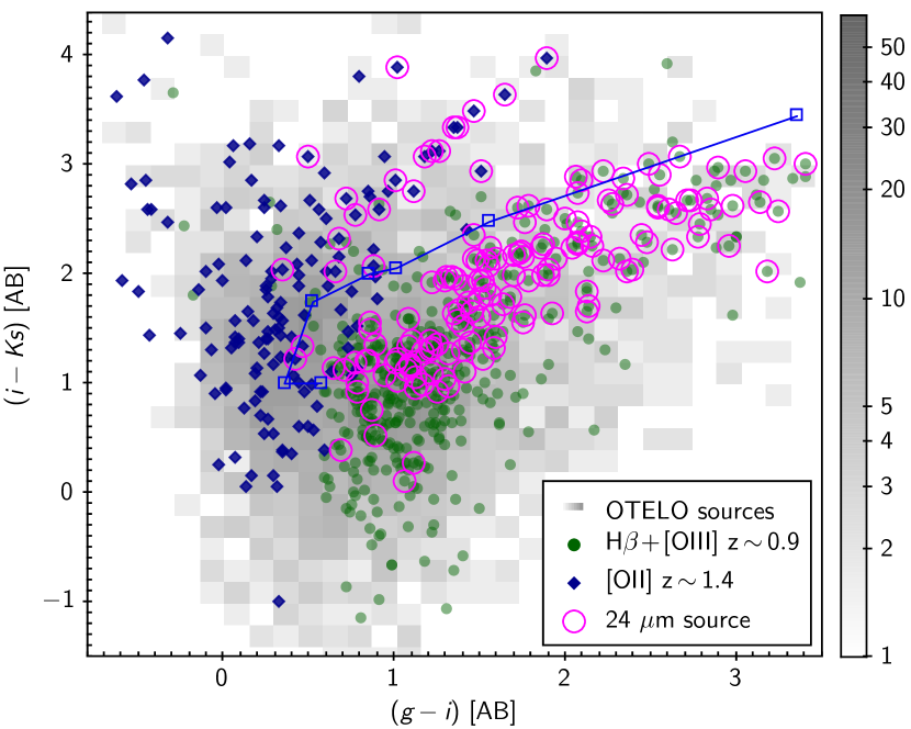
Figure 26: ($i-K_{S}$) versus ($g-i$) colour-colour diagram showing the H$\beta$+[OIII]$\lambda$4959,5007 (filled circles) and [OII]$\lambda$3726,3729 (filled diamonds) emission-line candidates at z$\sim$0.9 and 1.4, respectively, selected as explained in the text. The grey background grid represents the OTELO sources and the open circles represent those sources detected with MIPS 24$\,\mu m$. As a reference, the blue line represents a colour sequence of selected galaxy templates, described in Section 5.5, from E/S0 type to SB1 (open squares) at redshift z = 1.15 and E($B$-$V$)=0. The reddest segment of this sequence is concurrent with the intrinsic attenuation axis.

According to Table 9 nearly 240 ELS candidates, distributed between [NeV]$\lambda$3426 and MgII hosts, can be found at $\sim$1.5 $<$ z $<$ 2.5. In this case, a colour diagram like the BzK plot (Daddi et al., 2004) would be appropriate to confirm the selection and classification of star-forming galaxies, passive-evolved ones at z $<$ 1.4, and stars, whilst old galaxies at z $>$ 1.4 would occupy the reddest corner of the plot. Figure 27 show a BzK-equivalent diagram but using the gzK_s filter system, following the offsets and colour cuts established by (Arcila-Osejo & Sawicki, 2013) for CFHTLS and WIRDS data.

All MgII ELS and 77% of [NeV]$\lambda$3426 candidates fall inside the region corresponding to star-forming galaxies (s-gzK_s) at z $>$ 1.4, and 85% of the sources classified as bona fide stars in Section 6.1 occupy the expected region in this diagram.

The [NeV]$\lambda$3426 are distributed in a colour sequence running along the colour cut between the s-gzK_s and passive-evolved galaxies at z $<$ 1.4. As other high ionization lines, [NeV]$\lambda$3426 is produced in the narrow-line region (NLR) of AGN (Vignali et al., 2014). It follows that OTELO’s [NeV]$\lambda$3426 ELS population would mainly correspond to narrow-line AGN having Seyfert-like optical spectra with a star-forming component as found at z $<$ 1.2 by Mignoli et al. (2013) in the zCOSMOS-Bright Survey, or by Vergani et al. (2017) in the VIMOS Public Extragalactic Redshift Survey (VIPERS). In the latter case, the authors state that [NeV]$\lambda$3426-emitting galaxies populate the blue cloud, the green valley or the red sequence, depending on the stellar mass and the age of the stellar populations of the host galaxy. This fact could explain the distribution of [NeV]$\lambda$3426 ELS candidates in Figure 27, which in turn may be understood by the existence of a causal relation between AGN activity and the mechanisms that regulate star formation phenomena. All these contributions will provide a robust reference population for further evolutionary analysis of the star formation-AGN connection, using the confirmed [NeV]$\lambda$3426 emitters from OTELO.

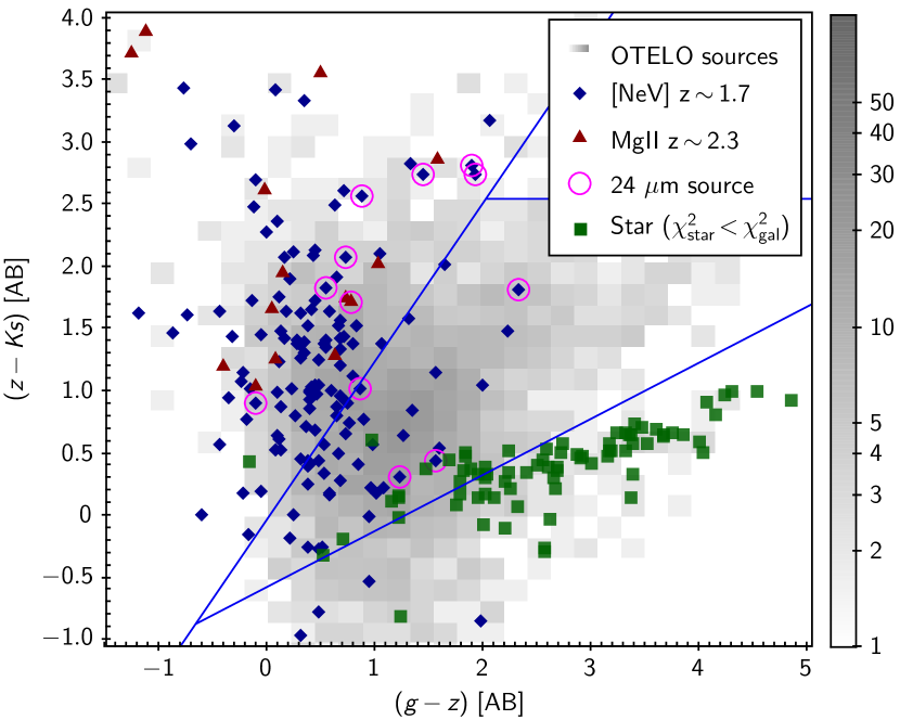
Figure 27: ($z-K_{S}$) versus ($g-z$) colour–colour diagram showing the [NeV]$\lambda$3426 (filled diamonds) and MgII (filled triangles) emission-line candidates selected as explained in the text. This diagram is based on the adaptation (Arcila-Osejo & Sawicki, 2013) for CFHTLS and WIRDS data of the BzK technique (Daddi et al., 2004) used to select star-forming galaxies at 1.4 $<$ z $<$ 2.5. According to this, the left side of the diagram would be occupied by the latter, and the central triangular region by passively evolved galaxies at z $<$ 1.4. The colour cut between these regions matches with the reddening axis. The lowest region of the diagram would be populated by stars. The OTELO star candidates, obtained as described in Section 6.1, are symbolized by filled squares. The grey background grid represents the OTELO sources and the open circles represent those sources detected with MIPS 24$\,\mu m$.

Going to redder broad bands in the multi-wavelength catalogue and using X-ray data, Figure 28 shows remarkable OTELO sources in the IRAC colour–colour plot. As expected, most of the point-like sources detected in the four MIR bands (96 from the total 191: Section 6.1) are grouped around the colour (3.6$\,\mu$m - 4.5$\,\mu$m) = -0.47, which corresponds to the zero-point of the Vega system. From 44 sources detected in both X-ray and MIR bands, 24 are within the AGN selection polygon from Stern et al. (2005), and 11 of the remaining ones are close to its limits. Such sources could also qualify as AGN host galaxies. This selection box include 12 point-like sources that could be considered as clear QSO candidates.

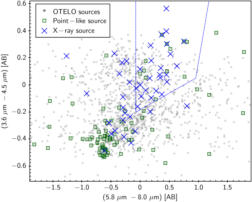
Figure 28: IRAC data colour distribution of the final OTELO catalogue. Open green squares represent sources classified as point-like sources as explained in Section 6.1, whilst blue crosses are the X-ray sources from the Pović et al. (2009) catalogue. The dotted line bounds the region of MIR-selected AGN from Stern et al. (2005).

6.4 Galaxy number counts

The contribution to the extragalactic background light at a given wavelength over large look-back time ranges may be estimated from the galaxy number counts. Starting from early works of Tinsley (1977) or Tyson (1988), up to the galaxy count statistics obtained for domains as dissimilar as X-ray (Harrison et al., 2016) and millimetre (Aravena et al., 2016), the surface density of galaxies as a function of the apparent flux provides insights not only into plausible scenarios that explain their evolution, but even as primary cosmological probe. In the case of OTELO, galaxy number counts may be useful as a basic sensitivity test when compared with similar surveys in depth and observed wavelength.

Excluding stars, observed and completeness-corrected (Section 4.3) number density counts for the raw extended source set (10839 entries of the OTELO multi-wavelength catalogue) is shown in Figure 29 (top panel). Instead of including galaxy count predictions from analytic or numerical models for comparison purposes, the completeness-corrected number counts from Subaru Deep Field (SDF) in the z-band (Kashikawa et al., 2004), and from Subaru/XMM-Newton Deep Survey (SXDS) in NB921 narrow-band (Ouchi et al., 2010), are also represented. The number count statistics from OTELO are not corrected by cosmic variance effects (which should be noticeable mainly on the bright side of the number density distribution), or by possible false-positive contaminants (which increase markedly for fainter magnitudes than AB $\sim$ 25, as shown in Figure 7). On the other hand, a cosmic variance correction is assumed for the differential counts from both SDF and SXDS data, regarding the large area surveyed in contrast to OTELO. Under these hypotheses, the OTELO to Subaru-related number count ratios are shown in Fig. 29 (bottom panel). On the bright side (AB $<$ 21.5), the number counts of OTELO show a mean excess of about 35% with respect to SDF statistics that would be attributed to cosmic variance. Up to 98% of this galaxy subsample is distributed in redshift below z${}_{\rm\,phot}$=1. Following Somerville et al. (2004), we consistently obtained an upper limit of the relative cosmic variance $\sigma_{\rm v}=b\,\sigma_{\rm DM}\simeq$ 0.38, with a bias $b\simeq$ 1.25 for a comoving number density of 0.0033 Mpc^-3, and a $\sigma_{\rm DM}\simeq$ 0.30 for the sampled comoving volume up to this redshift. On the faint end of the number count distribution (AB $>$ 24.5), a mean excess between 32% and 37% with respect to SDF and SXDS data, respectively, can be appreciated in Figure 29. From testing different approaches for possible false-positive source rejection, such apparent excess in the number counts with respect to other surveys tends to dissapear. As evident, the Poissonian uncertainties assigned to the number counts of this survey (Fig. 29, top) are certainly smaller than the differences which explanations are tried above.

Depending on the magnitude range, the behaviour of all these NIR galaxy counts can be fitted by power-laws whose slopes are sensitive to varied effects that include those cited above. In the case of OTELO and SDF, the bright and faint ends of the galaxy count trends are well approximated by power-law pairs with an elbow at around AB = 21, which is consistent with previous studies in this spectral regime (see for example Gardner et al., 1993; Prieto & Eliche-Moral, 2015; Stefanon et al., 2017). The AB magnitude upper limit fit corresponds to $\sim$ 50% completeness in all the sets represented. Number count slopes $\gamma$ from best-fitting in each case are given in Table 12.

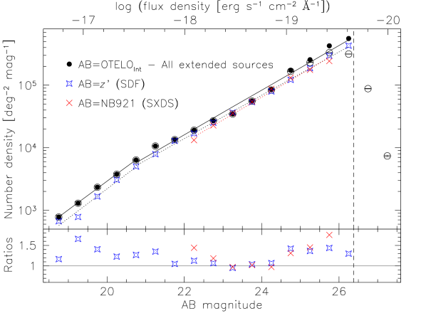
Figure 29: Number counts of the OTELO raw extended sources observed (open symbols) and corrected by completeness (filled symbols) according to the results presented in Section 5. Error bars are confined to Poisson statistics and the dashed line mark the 50% completeness limiting flux, which was adopted as the significance limit for the completeness correction. In comparison, blue stars and red crosses mark the faintest total number counts (corrected) reported by Kashikawa et al. (2004) (z’-band; SDF) and Ouchi et al. (2010) (NB-921; SXDS), respectively.

Table 12: Number count slopes from data fitting in Figure 29.

Survey/band	Magnitude	Slope ($\gamma$)
	range [AB]
OTELOInt	18.0-21.0	0.458 $\pm$ 0.008
–	21.0-26.4	0.357 $\pm$ 0.012
SDF / $z^{\prime}$	18.0-21.0	0.468 $\pm$ 0.046
SDF / $z^{\prime}$	21.0-26.5	0.346 $\pm$ 0.004
SXDS / NB921	22.0-26.0	0.363 $\pm$ 0.013

7 Discussion and conclusions

The OTELO survey is the deepest emission–line survey to date, being unique in terms of minimum detectable flux and emission–line equivalent width. OTELO demonstrates the power of narrow-band imaging by using low spectral resolution tunable filters as implemented in the OSIRIS instrument at the 10m GTC.

The first pointing of the survey was a 7.5′$\times\,$7.4′ ($\sim$0.015 square degrees) area in the EGS field. We scanned the spectral window from 9070 to 9280 Å, free of strong sky emission lines, with a total exposure time of 108 h. The first data product of the survey consists of 36 TF slices, according to the central wavelength, composed in turn of six narrow-band images of 12 Å bandwidth, with an overlap between contiguous images of 6 Å.

In this paper we present the final OTELO catalogue. OTELO sources have been obtained after using SExtractor on a Deep image built by combining all science frames. Specific algorithms have been developed to subtract sky rings, ghosts, and spurious artefacts from the RTF images. Astrometric calibration has been done carefully in order to align the individual science frames, resulting in an internal RMS better than 0.03″. The flux calibration has been obtained using two spectroscopic standard stars within the OTELO field.

From the 11237 raw entries, the OTELO catalogue contains 9862 objects at a 50% completeness AB-magnitude of 26.38, as measured in the OTELO-Deep image. The catalogue is complemented with ancillary catalogues coming from X-rays, UV, optical, mid- and far infrared. It is also cross-matched with CFHTLS and DEEP2 surveys to obtain either spectroscopic or complementary photo-z information.

Our photometric redshifts have been determined through the LePhare code, using libraries for normal and starburst galaxies, Seyferts, QSOs, and stars, including T brown dwarfs. The accuracy of the photometric compared to spectroscopic redshifts is better than $|\Delta$z$|$/(1+z) $\leq$ 0.2. Therefore, the OTELO catalogue has 9709 sources with non-null photo-z solutions, and 6600 of them have an uncertainty $\delta\,$z${}_{\rm\,phot}$ $<$ 0.2 (1+z${}_{\rm\,phot}$). This is a crucial step, as redshift information is needed to identify emission lines in the OTELO survey.

From the total number of sources detected, 81 are stellar candidates, probably with spectral types ranging from F3 through M7, with the luminosity class of dwarfs or subdwarfs, according to the Besançon model of the Galaxy (Robin et al., 2003). On the other hand, the number counts distribution of the OTELO extended sources is consistent with similar data given in literature whenever the effects of the relative cosmic variance and the fraction of possible false-positive contaminants are considered.

From the analysis of the pseudo-spectra, 5322 ELS candidates with line widths smaller than FWHM $\sim$ 60 Å are detected. Using a colour-excess technique, a total of 3226 candidates were segregated, from which 1542 were already detected using the pseudo-spectra. The total number of raw emitter candidates found is then 7006. It is important to note that the colour-excess technique complements the selection using TF pseudo-spectra, but that the colour-excess technique alone would miss more than 50% of the candidates to ELS. Also, another main result is that 16% of the objects (1812) from the raw catalogue are ELS candidates directly attributable to the strongest emission lines in the optical. This ELS population consists of objects emitting [SII], H$\alpha$+[NII], [OIII], H$\beta$, [OII], MgII, [NeV], and CIII], and [SII], at redshifts from 0.33 to 3.9. Other emission lines can be also identified by using photometric redshift distributions, such as HeII and Ly$\alpha$. Finally, another 483 objects are candidates to be absorption-line systems. These population of emitters and absorbers at different redshifts will be studied in forthcoming papers. The first release of the OTELO value-added products will be public on the second half of 2019.