Simulation-Driven Optimization of High-Order Meshes in ALE Hydrodynamics

Abstract

In this paper we propose tools for high-order mesh optimization and demonstrate their benefits in the context of multi-material Arbitrary Lagrangian-Eulerian (ALE) compressible shock hydrodynamic applications. The mesh optimization process is driven by information provided by the simulation which uses the optimized mesh, such as shock positions, material regions, known error estimates, etc. These simulation features are usually represented discretely, for instance, as finite element functions on the Lagrangian mesh. The discrete nature of the input is critical for the practical applicability of the algorithms we propose and distinguishes this work from approaches that strictly require analytical information. Our methods are based on node movement through a high-order extension of the Target-Matrix Optimization Paradigm (TMOP) of [1]. The proposed formulation is fully algebraic and relies only on local Jacobian matrices, so it is applicable to all types of mesh elements, in 2D and 3D, and any order of the mesh. We discuss the notions of constructing adaptive target matrices and obtaining their derivatives, reconstructing discrete data in intermediate meshes, node limiting that enables improvement of global mesh quality while preserving space-dependent local mesh features, and appropriate normalization of the objective function. The adaptivity methods are combined with automatic ALE triggers that can provide robustness of the mesh evolution and avoid excessive remap procedures. The benefits of the new high-order TMOP technology are illustrated on several simulations performed in the high-order ALE application BLAST [2].

1 Introduction

Lagrangian methods for compressible multi-material shock hydrodynamics [3, 4, 5, 6, 7] are characterized by a computational mesh that moves with the material velocity. A key advantage of using such methods is that they do not produce any numerical dissipation around contact discontinuities and material interfaces, when these are aligned with the element boundaries of the moving mesh. This is a consequence of the fact that the dynamics equations, when written in a Lagrangian frame, do not include nonlinear convective terms. However, the main disadvantage of Lagrangian methods is that they lead to mesh distortion, which results in small time steps or simulation breakdowns. Many problems of interest, i.e., impact simulations, cannot be run to longer evolution times by a purely Lagrangian method. These disadvantages are addressed by the Arbitrary Lagrangian-Eulerian (ALE) approach [8, 9, 10, 11], which involves the notion of periodic mesh optimization. However, while improving the mesh, ALE methods can produce their own numerical errors around the material interfaces, thus counteracting the main advantage of the Lagrangian approach.

In this paper we propose mesh optimization methods that provide mechanisms to control the amount of numerical error resulting from the ALE approach. Keeping unchanged the method’s underlying solution transfer (remap) and Lagrangian phases, we explore how mesh adaptivity through node movement (a.k.a. $r$-adaptivity), adaptive ALE triggers, and restricted node movement can be used to decrease the errors resulting from the overall ALE procedure. This paper extends our previous work on ALE hydrodynamics in the BLAST code [12, 13, 14] and mesh optimization by the Target-Matrix Optimization Paradigm [1, 15]. We incorporate the TMOP technology in the context of a high-order finite element ALE approach for multimaterial flow and introduce several important notions, including limiting of node movement based on the simulation dynamics, proper normalization of the energy functional, adaptivity to discrete simulation features, and adaptive ALE triggers. We focus on high-order curved meshes which have recently shown several mathematical and computational advantages, including optimal convergence rates on domains with curved boundaries/interfaces, symmetry preservation in radial flow [12, 16] and equivalent simulation quality with a smaller number of degrees of freedom [12, 17, 18].

Although in this paper we consider a particular application (BLAST), an important aspect of the TMOP approach is its generality. In particular, our methods are fully algebraic and do not involve any low-level geometric manipulations. They only require information about the local Jacobians, and thus can be applied to meshes of any order (including linear meshes), element type, and dimension. The proposed methods can be applied to both monolithic ALE methods [19, 20, 21] to define their mesh velocity, and ALE methods that split the Lagrangian, mesh optimization and remap phases. They can also be applied to diffused interface methods, where ALE errors are decreased by shrinking the transition region of the volume fraction functions, or exact interface representation methods [22], where ALE errors can be decreased by obtaining better mesh resolution in the interface regions.

The algorithms presented in this paper rely strictly on node movement and preserve the original topology of the mesh. Reconnection-based remesh approaches are more powerful in terms of controlling the mesh characteristics, but also require more complicated solution transfer procedures, see [23].

Our mesh optimization method is based on the TMOP framework described in [15, 24, 25]. This approach is distinguished from similar methods by its emphasis on target-matrix construction methods that permit a greater degree of control over the optimized mesh. Pointwise mesh quality metrics are defined by utilizing sub-zonal information obtained by sampling element Jacobians at element quadrature points. These metrics are capable of measuring shape, size or alignment of the region around the point of interest. TMOP requires predefined target-matrices as a way for the user to incorporate application-specific physical information into the metric that is being optimized. The combination of targets and quality metrics is used to optimize the node positions, so that they are as close as possible to the shape, size and/or alignment of their targets.

The rest of the paper is organized as follows. In Section 2 we review the multi-material ALE hydrodynamics framework in BLAST and the basic TMOP components. Section 3 describes the TMOP optimization functional in further detail, along with the concepts of limited node motion and proper normalization of the resulting nonlinear functional. Mesh adaptivity to discrete simulation features and its relation to dynamic ALE triggers is discussed in Section 4. Section 5 presents several numerical tests that demonstrate the features of the discussed methods. Conclusions are presented in Section 6.

2 Preliminaries

In this section we provide a brief overview of the multi-material ALE framework (as implemented in the BLAST code) that is used to test the proposed mesh optimization methods. We focus only on aspects that are relevant to our mesh optimization purposes, while a complete description of our ALE hydrodynamics methods can be found in [14]. We also provide a summary of the basic TMOP components in the context of BLAST.

2.1 Multi-Material ALE Framework

BLAST solves the multi-material Euler equations by clearly separating the Lagrange, remesh and remap phases. It utilizes a single-fluid multi-material description of the system where all materials share a common velocity, but each has its own density and energy. BLAST supports performing an arbitrary number of Lagrangian steps between two ALE steps (remesh+remap), as opposed to continuous remap algorithms that perform an ALE step after every Lagrangian step.

Space discretization

The space discretization is based on high-order finite elements. Velocity $v$ is discretized in the finite element space $\mathcal{V}\subset[H^{1}(\widehat{\Omega})]^{d}$, with basis $\{w_{i}\}$, where $\widehat{\Omega}$ is the computational mesh corresponding to the domain of interest $\Omega$, and $d$ is the space dimension. Specific internal energies $\{e_{m}\}$ are discretized in $\mathcal{E}\subset L^{2}(\widehat{\Omega})$, with basis $\{\phi_{j}\}$, where $m$ is the material index. Material densities $\{\rho_{m}\}$ are evolved at certain quadrature points of interest through the notion of pointwise mass conservation. Throughout this manuscript we refer to the pairs of spaces $Q_{k}Q_{k-1}$, by which we denote $\mathcal{V}=(Q_{k})^{d}$, i.e., the Cartesian product of the space of continuous finite elements on quadrilateral or hexahedral meshes of degree $k$, and $\mathcal{E}=\hat{Q}_{k-1}$, the companion space of discontinuous finite elements of order one less than the kinematic space. As shown in [12] the specific choice of $Q_{1}Q_{0}$ corresponds to traditional staggered grid discretizations under additional simplifying assumptions.

Discrete mesh representation

To obtain a discrete representation of the high-order mesh, we start with the set of kinematic scalar basis functions $\{\bar{w}_{i}\}_{i=1}^{N_{w}}$ on a reference element $\bar{E}$. The shape of any element $E$ in the mesh is then fully described by a matrix $\mathbf{x}_{E}$ of size $d\times N_{w}$ whose columns represent the coordinates of the element control points (a.k.a. nodes or element degrees of freedom). Given $\mathbf{x}_{E}$, we introduce the map $\Phi_{E}:\bar{E}\to\mathbb{R}^{d}$ whose image is the high-order element $E$:

$$x(\bar{x})=\Phi_{E}(\bar{x})\equiv\sum_{i=1}^{N_{w}}\mathbf{x}_{E,i}\bar{w}_{i}(\bar{x})\,,\qquad\bar{x}\in\bar{E},$$ (1)

where we used $\mathbf{x}_{E,i}$ to denote the $i$-th column of $\mathbf{x}_{E}$. To ensure continuity between mesh elements, we define a global vector $\mathbf{x}$ of mesh positions that contains the $\mathbf{x}_{E}$ control points for every element. For any element $E$ in the mesh, we can compute the Jacobian of the mapping $\Phi_{E}$ at any reference point $\bar{x}\in\bar{E}$ as

$$A_{E}(\bar{x})=\frac{\partial\Phi_{E}}{\partial\bar{x}}=\sum_{i=1}^{N_{w}}\mathbf{x}_{E,i}[\nabla\bar{w}_{i}(\bar{x})]^{T}\,.$$ (2)

We will refer to the initial mesh, which is to be optimized, as the Lagrangian mesh. We denote the Lagrangian mesh by $\mathcal{M}_{0}$.

Material representation and evolution

Material positions are represented on a discrete level as point-wise volume fractions at certain quadrature points of interest. At any such quadrature point $x$, the volume fraction values $\{\eta_{m}\}$ satisfy $\eta_{m}(x)\geq 0$ and $\sum_{m}\eta_{m}(x)=1$. During the Lagrange phase, these volume fraction are evolved by a sub-zonal closure model, see [13]. Before each remap procedure, these quadrature point values are projected to discontinuous $L^{2}$ functions, which are remapped, by solving an advection-based PDE, to the new mesh. Once the remap step is complete, the remapped $L^{2}$ functions are interpolated back to the quadrature points of interest. The above ALE treatment of the material positions leads to numerical diffusion around the material interfaces, which is often the main source of numerical dissipation error in BLAST.

2.2 Overview of TMOP

Mesh optimization in TMOP is driven by moving the mesh nodes (i.e. changing the values of the vector $\mathbf{x}$) in a way that minimizes a mesh quality metric, $\mu(T)$, over the computational mesh. In this section we explain the meaning of $\mu$ and $T$. A more detailed discussion about the TMOP optimization functional is presented in Section 3.

The weighted Jacobian matrix $T$ represents the transformation from a target configuration to the current physical (or active) mesh positions, so that a perfect mesh would result in $T=I$. At each quadrature point, the matrix $T$ is determined using two Jacobian matrices:

• The target-matrix $W_{d\times d}$, which is the Jacobian of the transformation from the reference to the target coordinates. This matrix is defined according to a user-specified method prior to optimization; it defines the desired local properties of the optimal mesh.

• The Jacobian matrix $A_{d\times d}$ of the transformation between reference and physical space coordinates, always computed by (2).

Then we have $T=AW^{-1}$. Note that both $A$ and $W$ are space-dependent functions of the nodal coordinates. As any Jacobian matrix, $W$ can be written as a decomposition of matrices that represent its main geometric properties:

$$W=[\text{volume}][\text{orientation}][\text{skew}][\text{aspect ratio}].$$ (3)

The concept of target construction allows the user specify some of the above components, and thus control the desired geometric property [25]. We utilize this concept further in Section 4 to achieve simulation-based mesh adaptivity.

Figure 1: Schematic representation of the major TMOP matrices.

Given a matrix $T=AW^{-1}$, the purpose of the local quality metric $\mu(T)$ is to measure the differences between $A$ and $W$ only in one or more particular components of (3), while being invariant of the others. The choice of quality metric is based on the geometric aspects that the user wants to control. For example, $\mu_{2}=\mid T\mid^{2}/2\tau-1$ is a shape metric that controls skew and aspect ratio, but is invariant to orientation and volume. Here, $\mid T\mid$ is the Frobenius norm of $T$ and $\tau=\text{det}(T)$. Similarly, $\mu_{7}=\mid T-T^{-t}\mid^{2}$ and $\mu_{9}=\tau\mid T-T^{-t}\mid^{2}$ are shape$+$size metrics that controls volume, skew and aspect ratio, but are invariant to orientation. The reader is referred to [15] for a more detailed discussion on quality metrics.

3 Recent Improvements in TMOP

In this section we go deeper into the details of the TMOP’s nonlinear objective function and present several improvements over our previous formulation presented in [15, 24]. These modifications are motivated by practical concerns related to restricting node movement and proper normalization of the different terms in the objective function.

3.1 Objective Function

TMOP optimizes the mesh quality by minimizing a global objective function $F(x)$ that depends on the local quality measure throughout the mesh. This minimization is performed by solving $\partial F/\partial\mathbf{x}=0$ with Newton’s method. The objective function has the following general form:

$$F(x)=\frac{1}{n}\sum_{s=1}^{n}\frac{\sum_{E(x)}\int_{E_{t}}{\omega}_{s}(x)\mu_{i_{s}}(T(x))dx_{t}}{\sum_{E(x_{0})}\int_{E_{t}}{\omega}_{s}(x_{0})\mu_{i_{s}}(T_{0}(x_{0}))dx_{t}}+c\sum_{E}\int_{E_{t}}\xi(x-x_{0},\delta(x_{0}))dx.$$ (4)

The right-most term is used to limit the node displacements during optimization. This term is discussed in Section 3.2. The other term represents an explicit combination of $n$ mesh quality metrics $\mu_{i_{1}},\dots\mu_{i_{n}}$. Although most problems require only one metric ($n=1$), in other cases [26] it might be necessary to combine metrics with different weights ${\omega}$ in order to make some of them more dominant in certain regions of the domain. The integrals in (4) are computed as

$$\sum_{E\in\mathcal{M}}\int_{E_{t}}{\omega}(x_{t})\mu(T(x_{t}))dx_{t}=\sum_{E\in\mathcal{M}}\sum_{x_{q}\in E_{t}}w_{q}\,\det(W(\bar{x}_{q}))\,{\omega}(x_{q})\mu(T(x_{q})),$$ (5)

where $\mathcal{M}$ is the current mesh, $E_{t}$ is the target element corresponding to the physical element $E$, $w_{q}$ are the quadrature weights, and the point $x_{q}$ is the image of the reference quadrature point $\bar{x}_{q}$ in the target element $E_{t}$. Note that the right-hand side in (5) depends on the mesh positions $x$ through the Jacobian matrices $A$ used in the definition of $T$. The integration in (5) is performed over the target elements, enforcing that the integral contribution from a given element $E$, relative to the contributions from other elements, is only based on the difference with its target $E_{t}$ (which is measured by $\mu(T)$), and not on its relative size compared to the other elements. In particular, very small elements will not be neglected by the optimization process due to their size. The existence of a minimum for variational optimization problems like (5) has been explored theoretically in [27, 28].

In general, the various quality metrics $\mu_{i}$ have different magnitudes; we have observed orders of magnitude differences in the resulting integrals. The role of the denominators in the first sum of (4) is to normalize the magnitude of the different metrics. The sum of the metric terms is always equal to $1$ at the start of the optimization process and is expected to decrease during the iteration. Furthermore, all metric integrals start at the same value of $1/n$. This normalization also makes the magnitude of each metric integral invariant of $i$, the level of refinement, the specifics of the problem (e.g. the units system), and the size of the domain.

3.2 Limiting of Node Displacements

One advantage of the Lagrangian approach is that it provides a natural form of mesh adaptivity. For example, the mesh spacing usually gets compressed around shock regions. Thus, it might be beneficial to have the ability to preserve, up to some extent, the positions $x_{0}$ of the Lagrangian mesh $\mathcal{M}_{0}$. Another important benefit of staying close to the Lagrangian mesh is minimizing errors due to remap. The purpose of the limiting term (the right-most term in in (4)) is to restrict the movement of nodes during the mesh optimization procedure with respect to their initial positions $x_{0}$. Note that the limiting term is space-dependent, allowing the preservation of mesh features (e.g. initial resolution) in specific regions of the domain, which is an important requirement for various applications [26]. A simple motivational 2D example is shown in Figure 2, where the goal is to preserve the resolution around the central boundary layer, while achieving uniform mesh resolution in the rest of the domain.

$\begin{array}[]{ccc}\includegraphics[width=184.9429pt]{figures/cyl_original}&\includegraphics[width=184.9429pt]{figures/cyl_limiting}\\ \end{array}$

Figure 2: Original mesh (left) and optimized mesh (right) through space-dependent restriction of the node displacements.

In what follows, we rely on the fact that there exists a bijective map between every position $x$, in the current mesh $\mathcal{M}$, and its initial position $x_{0}$ in the Lagrangian mesh $\mathcal{M}_{0}$, which is the case in methods based on node movement. We define the limiting term from (4) as a general function of distance between the current positions $x$ and their corresponding Lagrangian positions $x_{0}$ as

$$c\sum_{E}\int_{E_{t}}\xi\left(x-x_{0}[x],\delta(x_{0}[x])\right),$$ (6)

where $\delta(x_{0})>0$ is a space-dependent scalar function that specifies the acceptable amount of displacement for each mesh node. Note that moving a given position $x$ changes the displacement $x-x_{0}$, but it does not change its image on the initial mesh $x_{0}[x]$ and the value of $\delta(x_{0}[x])$. The values of $\delta$ are problem-specific and must be specified by the user. For example, in the remesh phase of ALE simulations, $\delta(x_{0})$ can be some fraction of the displacement that occurs between the last two ALE steps.

To achieve the limiting effect, the function $\xi$ has the following properties:

1. $\xi\rightarrow 0$ when $x\rightarrow x_{0}$, and in particular, the initial value of the limiting integral is negligible.

2. $\xi$ is an increasing function with respect to $|x-x_{0}|$, i.e., the limiting term grows for bigger displacements.

3. $\xi(x-x_{0},\delta)=1\iff|x-x_{0}|=\delta$. This property is used to give the users a physical intuition of the meaning of $\delta$, i.e., the limiting term will start to dominate the objective function whenever the mesh nodes move to a distance of $\delta$, or bigger, from their original positions. Note that, due to their normalization, the metric integrals of (4) are always expected to be in $[0,1]$.

4. $\xi$ has two well-defined derivatives with respect to ${\bf x}$. This enables us to use a standard Newton-based nonlinear solver.

5. $\xi$ is unitless, i.e., it is invariant to rescaling of the domain or change of the physics units system.

The rate at which the limiting term starts to influence the objective function $F(x)$ depends on the particular form of $\xi$. Our tests usually utilize one of the following two formulas:

$$\xi_{1}=\frac{\lvert x-x_{0}\rvert^{2}}{\delta^{2}},\quad\xi_{2}=e^{10\left(\frac{\lvert x-x_{0}\rvert^{2}}{\delta^{2}}-1\right)}.$$ (7)

As shown in Figure 3, the exponential option $\xi_{2}$ becomes active, and starts to grow much faster, only after mesh displacement approaches the maximum allowed value of $\delta$.

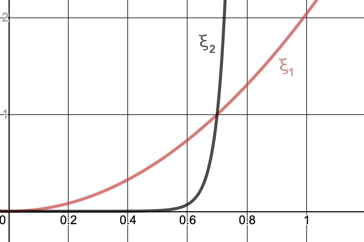
Figure 3: Graphs of $\xi_{1}$ (red) and $\xi_{2}$ (black) for $\delta=0.7$.

The constant $c$ in equation (6) provides proper normalization. In particular, note that the integrals in (6) are over target elements, which may or may not have the notion of size. For example, it is not necessary to set the local volume of a target element which will be used to perform shape-only optimization. To preserve invariance under mesh refinement, we set $c$ to

$$c=\begin{cases}\frac{1}{N_{E}V_{\Omega,avg}}=\frac{1}{V_{\Omega}}&\text{if the targets contain volumetric information},\\ \frac{1}{N_{E}}&\text{otherwise},\end{cases}$$ (8)

where $N_{E}$ is the total number of elements in the mesh, and $V_{\Omega}$ is the total volume of the domain.

A simple 2D example that demonstrates the desired behavior of the normalization factors under mesh refinement is presented in Figure 4 and Table 1. In this example we optimize a third order mesh towards ideal shape equally-sized targets with the shape+size metric $\mu_{9}=\tau\mid T-T^{-t}\mid^{2}$. Node displacements are restricted by using $\xi_{1}$ and $\delta(x_{0})=0.1$. We observe similar behavior for the different mesh resolutions.

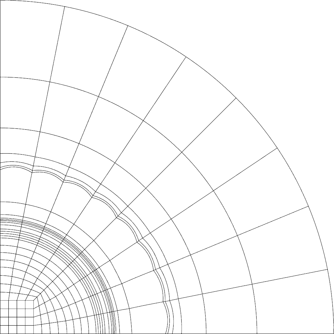
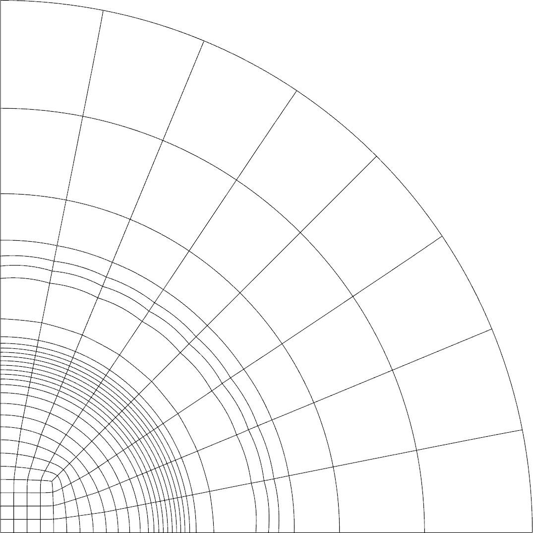
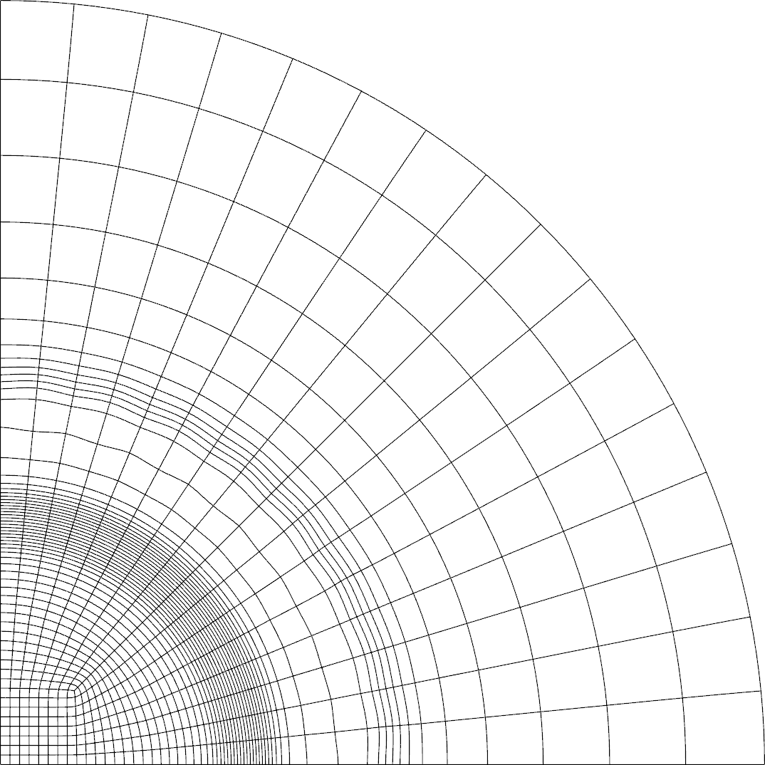
Figure 4: Perturbed initial mesh (left) and optimized meshes using $\mu_{9}$ and $\xi_{1}$ with $\delta(x_{0})=0.1$ for 0,1,2 refinements of the original mesh

Refinements	Final $F$	Metric part	Limiting part	Max displacement
0	0.8423	0.7819	0.0604	0.0083
1	0.8422	0.7819	0.0602	0.0083
2	0.8422	0.7819	0.0602	0.0083

Table 1: Results for final functional value $F$ and its components for several refinements of the $Q_{3}$ ICF mesh, using $\mu_{9}$ and $\xi_{1}$ with $\delta(x_{0})=0.1$.

Local mesh optimization

A standard approach to perform local mesh optimization is to eliminate unknowns on the linear algebra level, i.e., to apply the Newton solver on a submesh. When the region of interest changes dynamically in ALE simulations, however, refactoring the linear algebra problem at every remesh step can be cumbersome. Another application of the space-dependent coefficient $\delta(x_{0})$ is that it can be used to perform local mesh optimization. This is demonstrated by another simple 2D test in Figure 5. Again we use a third-order mesh, $\mu_{9}$, and ideal equally-sized targets, but in this case we vary the $\delta$ function in space through

$$\delta(x_{0})=\begin{cases}10^{-4}&\text{if }x>y\text{~{}(forcing strong limiting)},\\ 1.0&\text{otherwise (effectively no limiting)}.\end{cases}$$

We observe that the chosen metric is active only in the non-restricted region.

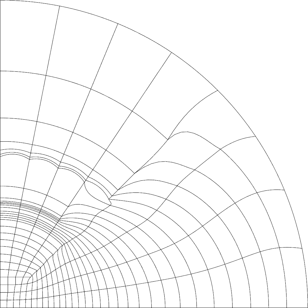
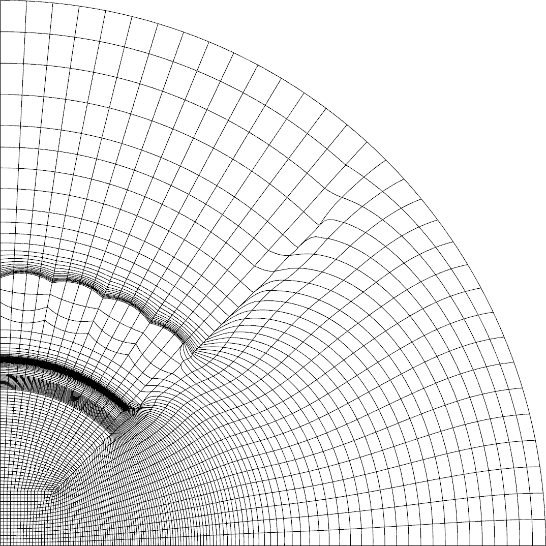
Figure 5: Perturbed initial mesh (left) and locally optimized meshes (0 and 2 refinements of the original mesh) using space-varying coefficient $\delta(x_{0})$.

Combination with ALE Hydrodynamics

As already mentioned, the above methods to restrict the node displacements, or perform local mesh optimization, are useful when one wants to preserve a certain feature that is available in the Lagrangian mesh. Our experience shows that it is a good practice to set $\delta(x_{0})$ to be some fraction of the displacement that occurs between the last two ALE steps, which we denote by $\delta_{L}(x_{0})$. This ties the amount of mesh relaxation to the amount of Lagrangian motion, and in particular, guarantees that nodes that do not move during the Lagrange phase ($\delta_{L}=0$), do not move in the remesh phase either. Various modifications can be performed to relax this restriction in certain problems, e.g., diffusing $\delta_{L}(x_{0})$ to obtain transition regions.

4 Mesh Adaptivity and ALE Triggers

Mesh adaptivity [29] is beneficial when a certain dynamic feature is not resolved by the Lagrangian mesh. In this section we demonstrate how the TMOP-based framework adapts the different geometric properties (3) of the high-order mesh to control the numerical errors in ALE methods. We start by describing the coupling between target construction and discrete simulation data, followed by a discussion of the appropriate triggering mechanisms in the remesh phase of ALE simulations.

4.1 Adaptivity to Discrete Simulation Fields

The objective of the r-adaptivity process is to optimize the mesh using information from a discrete function, e.g., a finite element solution function that is evolved during the Lagrangian phase. In TMOP, r-adaptivity is achieved by incorporating the discrete data into the target Jacobian matrices. This process can be split into five major steps:

1. Choice of adaptation goal, i.e., which geometric properties of the mesh must be controlled and what is their desired behavior. This can be motivated, for example, by known a-priori error estimates.

2. Derivation of geometric parameters from relevant simulation data.

3. Definition of pointwise target Jacobian matrices $W$.

4. Choice of a quality metric $\mu(T)$ that measures differences in the geometric quantities of interest.

5. Mesh optimization by solving the final nonlinear optimization problem.

The first two steps are simulation and problem-dependent, but once the geometric parameters are known, one can construct the targets and optimize the mesh automatically. Alternative approaches for linear meshes in the context of ALE hydrodynamics are described in [30, 31].

Next we provide a simple 2D example to illustrate the above procedure. Suppose we want to adapt the mesh size and aspect ratio to a material interface, and suppose that the material position is prescribed by a volume fraction function $\eta$, as it is the case in BLAST, see Figure 6. The needed geometric parameters can be computed from the gradient of $\eta$. The aspect ratio $r$ is computed by the ratio of the gradient components (i.e., $r\propto\nabla_{x}\eta/\nabla_{y}\eta$) and the local size $s$ depends on the magnitude of the gradient (i.e., $s\propto||\nabla\eta||$). To complete the definition of shape, we also choose the target skewness to be the same as that for an ideal element ($\phi=\pi/2$ for a quadrilateral element). Using this approach, we construct the target matrix $W$ corresponding to (3) as

$$W=\begin{bmatrix}\sqrt{s}&0\\ 0&\sqrt{s}\end{bmatrix}\begin{bmatrix}1&0\\ 0&1\end{bmatrix}\begin{bmatrix}1&\cos\,\phi\\ 0&\sin\,\phi\end{bmatrix}\begin{bmatrix}\frac{1}{\sqrt{r}}&0\\ 0&\sqrt{r}\end{bmatrix}.$$ (9)

Next we choose the shape+size metric $\mu_{9}$, which measures differences of size, aspect ratio, and skewness between target and physical configurations. This metric is invariant to orientation (note that $W$ sets targets that have no rotation, but this is irrelevant due to the choice of $\mu_{9}$). The final result for a third order mesh is presented in Figure 6 which shows that the mesh resolves the interface. Further details about target construction algorithms can be found in [25]. Note that the above procedure can be applied to various kinds of simulation data coming from the Lagrangian phase, e.g., shock positions, high temperatures, pressure gradients, etc. Alternative adaptivity approach, for the case when $\eta$ is prescribed analytically, is presented in [32]. We also stress the work presented in [33], where the authors utilize an approach similar to TMOP to adapt curved meshes in the context of steady-state Navier Stokes equations.

$\begin{array}[]{ccc}\includegraphics[height=130.08731pt]{figures/indicator}&\includegraphics[height=130.08731pt]{figures/indicator_opt}\\ \end{array}$

Figure 6: Material indicator function on the initial uniform mesh (left panel) and adaptively optimized mesh (right panel).

Discrete data on intermediate meshes

Since the discrete solution fields are available only on the Lagrangian mesh $\mathcal{M}_{0}$, adaptive mesh optimization requires a method to evaluate these fields on the intermediate meshes that are obtained during the Newton iteration. All simulations in this paper use the advection-based transfer as described in Section 4.2 of [24]. Another option is high-order interpolation between meshes, see Section 2.3 of [34] and Section 4.1 of [24].

Gradients of adaptive target matrices

As we use gradient-based nonlinear solvers to update mesh positions, we have to compute derivatives of $\mu(T=AW^{-1})$ with respect to $\mathbf{x}$. Since $W$ depends on a discrete function of the mesh positions, the derivatives $\partial W/\partial\mathbf{x}$ must be taken into account. The formulas for these derivatives and further discussion are presented in Section 3 of [24].

Combination of adaptivity and limiting of displacements

Since mesh adaptivity may require significant amounts of mesh displacements to achieve the desired geometric characteristics, including the limiting term (6) in the nonlinear functional can be counterproductive. Nevertheless, the limiting effects (e.g. local mesh optimization) can still be achieved by designing a proper space-dependent limiting function $\delta(x_{0})$, which must be aware of the adaptivity goals.

4.2 Adaptive ALE Triggers

We have briefly discussed ALE triggers in Section 5 of [24]. In this section we make several important improvements to the work presented in [24], along with a more detailed discussion.

Since BLAST can perform any number of Lagrangian steps between two ALE steps, an important question is when, or how often, to optimize the mesh. Ideally we want a trigger mechanism that does remesh often enough to avoid small computational time steps due to mesh distortion. At the same time we do not want to remesh too often, as ALE calculations can lead to increased numerical dissipation. In BLAST, this dissipation comes from transitions between primal and conservative variables and monotonicity treatment in the remap phase [14], which is a purely numerical process that is independent of the physics of the Euler equations. Furthermore, in the case of mesh adaptivity, higher number of remesh steps slow down the overall simulations as the mesh adaptivity process involves the extra computations explained in Section 4.1.

The above discussion suggests that the ALE trigger mechanism must be aware of the mesh quality during the Lagrangian phase, and induce an ALE step only when the mesh quality is below a certain threshold. It is important to note that mesh quality must be viewed in terms of the mesh quality metric used in the mesh optimization phase; the mesh optimization phase is expected to produce a mesh that is above the trigger threshold.

The TMOP concepts can be utilized to define such mesh optimization triggers, both in the purely geometric and the simulation-driven case. Similar to constructing target-matrices, the user specifies one or more admissible Jacobian matrix, $S$, which defines the transformation from the reference element to the worst element that can be used during the Lagrangian phase. Note that $S$ is initialized in the beginning and stays constant throughout the simulation. Then $U=SW^{-1}$ represents the Jacobian of the transformation between target and admissible coordinates, which is used to calculate $\mu(U)$, the highest admissible mesh quality metric value for the metric of interest. With that, remesh is triggered whenever $\mu(T)\geq\mu(U)$ at any mesh quadrature point. In the case of mesh adaptivity, the target matrices $W$ adapt in time as they depend on some dynamic solution fields. Thus $U$ and $\mu(U)$ change too, leading to a trigger that is adapted to the current Lagrangian solution.

For example, suppose we adapt small mesh size to high temperature regions. Then at a fixed point in space $x$, the admissible metric value $\mu(U(x))$ represents the admissible size deviation, given the current temperature at $x$. The value $\mu(T(x))$ represents the actual size deviation of the Lagrangian mesh, at the current temperature.

The specific formulation of $S$ is, of course, problem dependent, e.g., it can be used to trigger remesh steps whenever particular mesh configurations occur. Just as the target-matrices $W$, the admissible matrices can contain information about the local shape, size or alignment, at any quadrature point. As a simple 2D example, we can define $S$ as

$$S=\begin{pmatrix}1&0\\ 0&S_{22}\end{pmatrix}\,,\text{where }S_{22}>0\text{ is a user-specified parameter}\,.$$ (10)

When $\mu$ is a shape metric, remesh is triggered based on local aspect ratio. When $\mu$ is a shape+size metric, remesh is triggered based on local size and aspect ratio.

ALE triggers can be combined with the use of the limiting term (6), as long as the limiting distances $\delta(x_{0})$ are large enough to allow the optimization process to achieve $\mu(T)<\mu(U)$ at all quadrature points.

5 Numerical tests

In this section we report numerical results from the algorithms in the previous sections as implemented in the BLAST code [2]. The baseline TMOP methodology is part of the MFEM finite element library [35, 36], which is freely available at mfem.org. The application-specific target constructions, however, are only included in the BLAST implementation. All physical units in the following tests are based on the $(cm,g,\mu s)$ unit system.

In what follows, tests that adapt mesh size always utilize a size indicator function $g(x)$ with values in $[0,1]$, where values close to $1$ represent regions with smaller mesh size. Target matrices are constructed as

$$W(x)=[g(x)s+(1-g(x))\alpha s]^{1/d}I,$$ (11)

where $\alpha$ is a user-specified size ratio between big and small local size. Unless otherwise specified, we use $\alpha=10$ for all numerical tests. Such targets specify custom size, ideal shape, and zero rotation; in all tests we use metrics that are invariant of rotation. The small local size $s$ is approximated by taking into account the total volume $V$ of the domain, the volume $V_{g}$ occupied by $g(x)$, the number $N_{E}$ of available elements, and the specified $\alpha$:

$$\frac{V_{g}}{s}+\frac{V-V_{g}}{\alpha s}=N_{E}\,,\quad\text{where }\quad V_{g}=\int_{\mathcal{M}_{0}}g_{0}(x_{0})\,,~{}~{}V=\int_{\mathcal{M}_{0}}1\,.$$ (12)

The calculation of $s$ is performed once on the Lagrangian mesh $\mathcal{M}_{0}$.

5.1 Triple Point

Our first test is the 3-material Triple Point problem described in [12]. This test is used to compare different remesh strategies and demonstrate their advantages and drawbacks in terms of accuracy and computational performance.

We start by performing a purely Lagrangian simulation to time 3.5 and record the final position of one of the materials, see Figure 7. We take this Lagrangian position as the true solution, as there is no diffusion of the material interface. For every other test, we define error by measuring differences with the Lagrangian result, for the same material’s position. These differences are measured by sampling both solutions at $10000$ equidistant points over the domain. This sampling is a nontrivial procedure by itself, as it involves interpolation in physical space of high-order finite element functions on curved meshes; for this we use the methods from Section 2.3 of [34]. The reported error is the average difference over all points. All simulations utilize a $Q_{3}Q_{2}$ discretization s.t. the mesh is third order.

Table 2 lists all tested approaches. Most cases use a fixed frequency, so that an ALE step is performed every 50 Lagrangian steps. The limited tests optimize the mesh using the shape metric $\mu_{2}$ combined with the quadratic $\xi_{1}$ limiting function and $\delta(x_{0})=a\delta_{L}(x_{0})$, where $a=1/2$ or $a=1/3$, see Section 3.2. The adapted tests optimize the mesh using the shape+size metric $\mu_{7}$, so that material interface regions are assigned smaller mesh sizes. We report the total number of Lagrangian steps, ALE steps, remap advection steps (i.e., the total from within all ALE steps), the relative runtime (all tests use the same computer configuration), and the error in the material position due to numerical diffusion. The final material positions for several of the major options is shown in Figure 8.

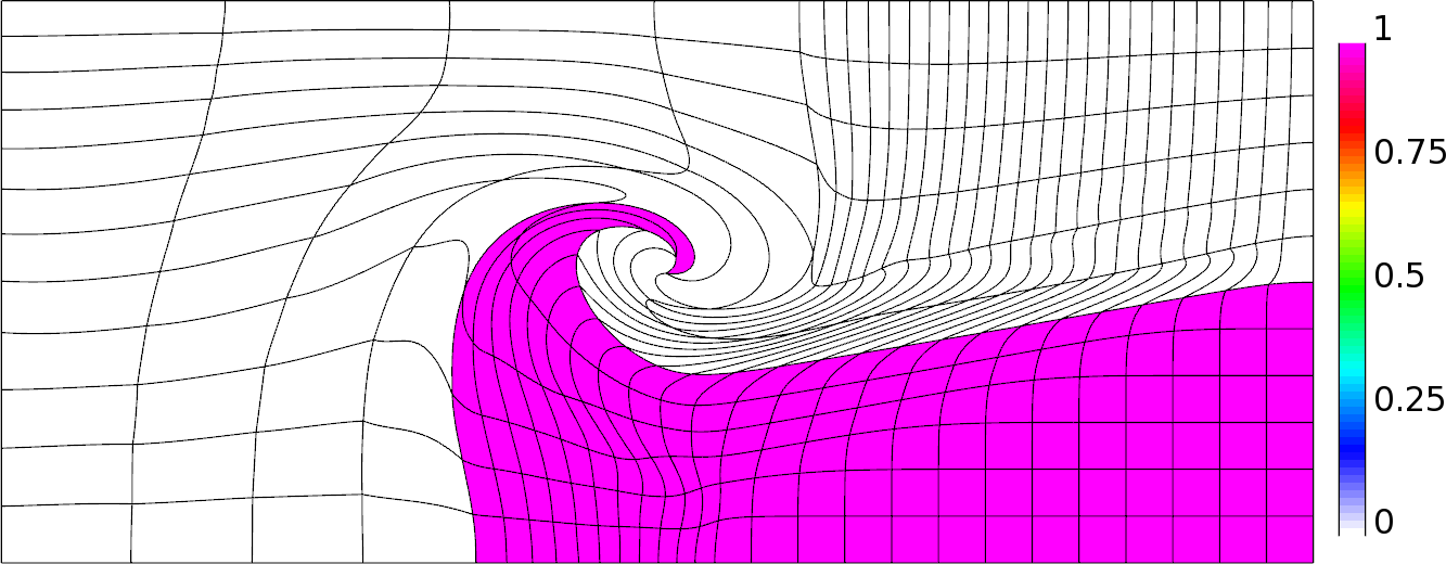
Figure 7: Mesh and material position resulting from a purely Lagrangian simulation.

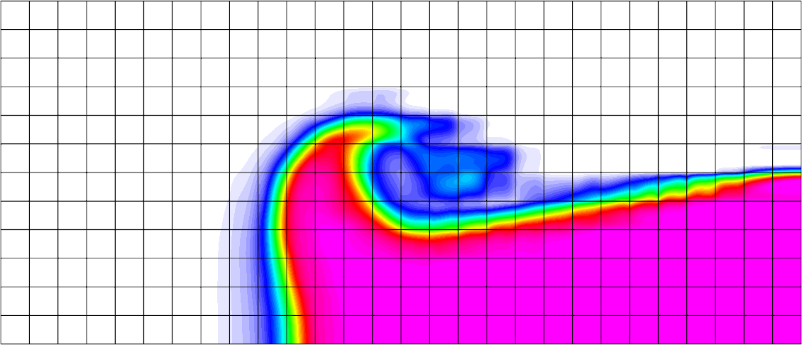
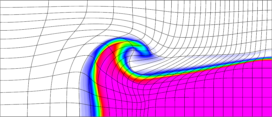
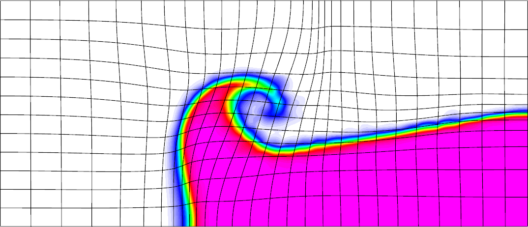
Figure 8: Meshes and material positions resulting from the Eulerian (left panel), limited by $\delta(x_{0})~{}=~{}1/2\delta_{L}(x_{0})$ (center panel), and adapted with automatic trigger (right panel) simulations.

Approach	# Lag	# ALE	# advect	runtime	error
Lagrangian	20808	0	0	615	0
Eulerian, period of 50	757	16	90	69	0.033
Limited $\frac{1}{2}$, period of 50	980	20	59	64	0.022
Limited $\frac{1}{3}$, period of 50	1505	31	55	86	0.020
Adapted, auto trigger	1666	8	137	174	0.017
Adapted, period of 50	1818	37	154	235	0.022

Table 2: Comparison between different ALE strategies for the Triple Point test.

We observe that the Eulerian approach, which always returns the mesh to its original configuration, is fast as it produces large Lagrangian time steps, but is also the most diffusive. Performing limiting with $a=1/2$ is a clear improvement over the Eulerian case, both in computational time and accuracy, because less advection remap steps are performed, which compensates the smaller size of the Lagrangian time steps. Decreasing the limiting distances by setting $a=1/3$ preserves the Lagrangian mesh more closely, resulting in smaller time steps and higher compute time. The error is slightly better, as less advection steps are performed.

Since the error in this test is always in the interface region, adapting the mesh size (with adaptive trigger) to this region is the most accurate approach. The automatic trigger is setup as in (10) with $S_{22}=4$, taking into account the local size and shape of any quadrature point in the mesh. For example, an ALE would be triggered whenever the local size differs by a factor of $\geq 4$ of the required mesh size, or the aspect ratio differs by a factor of $\geq 4$ of the ideal aspect ratio. Mesh adaptivity, however, leads to slower computations as it leads to bigger mesh displacements in the remesh phase, which leads to more advection steps in the remap phase.

As discussed in Section 4.2 performing mesh adaptivity with too frequent ALE steps can lead to both slower and more diffusive simulations. This is demonstrated by the last case in Table 2, where an ALE step is performed every 50 steps, independent of the mesh quality during the Lagrangian phase.

5.2 2D ALE Simulation of Gas Impact

This test represents a high velocity impact of gasses that was originally proposed in [37]. It involves three materials that represent an impactor, a wall, and the background. This problem is used to demonstrate the method’s behavior in an impact simulation that cannot be executed in Lagrangian frame to final time as it produces large mesh deformations.

The domain is $[0,2]\times[0,2]$ with $v\cdot n=0$ boundary conditions. The material regions are $0.15\leq x\leq 0.65$ and $0.9\leq y\leq 1.1$ for the impactor, $0.1\leq x\leq 1.0$ for the wall, and the rest is background. The initial horizontal velocity of the impactor is $0.2cm/\mu s$. The problem is run to a final time of $t=10$ on a $80\times 80$ second order structured mesh. The complete thermodynamic setup of this problem and additional details about our multi-material finite element discretization and overall ALE method can be found in [13, 14].

The goal of every ALE remesh step is to adapt the size of the mesh towards the locations of the impactor, the wall, and all material interfaces. The adaptivity field $g(x)$ is constructed from the simulation’s discrete volume fractions $\eta_{wall}$ and $\eta_{imp}$, and a reconstructed interface indicator function $\eta_{int}$:

$$g(x)=\max(\eta_{wall}(x),\eta_{imp}(x),\eta_{int}(x))\,,$$

where the range of all $\eta$ functions is $[0,1]$. Target Jacobians $W(x)$ are constructed by (11), and the shape+size metric $\mu_{7}$ is used to optimize the mesh. An automatic ALE trigger is utilized by setting $S_{22}=4$ in (10).

The time evolution of the material positions and the corresponding mesh is demonstrated in Figure 9. This calculation required 49400 Lagrange time steps, 38 ALE steps, and 760 advection remap steps in total. We observe that the algorithm adapts well to the moving materials and the interface regions, while preserving good overall shape throughout the domain.

   

   

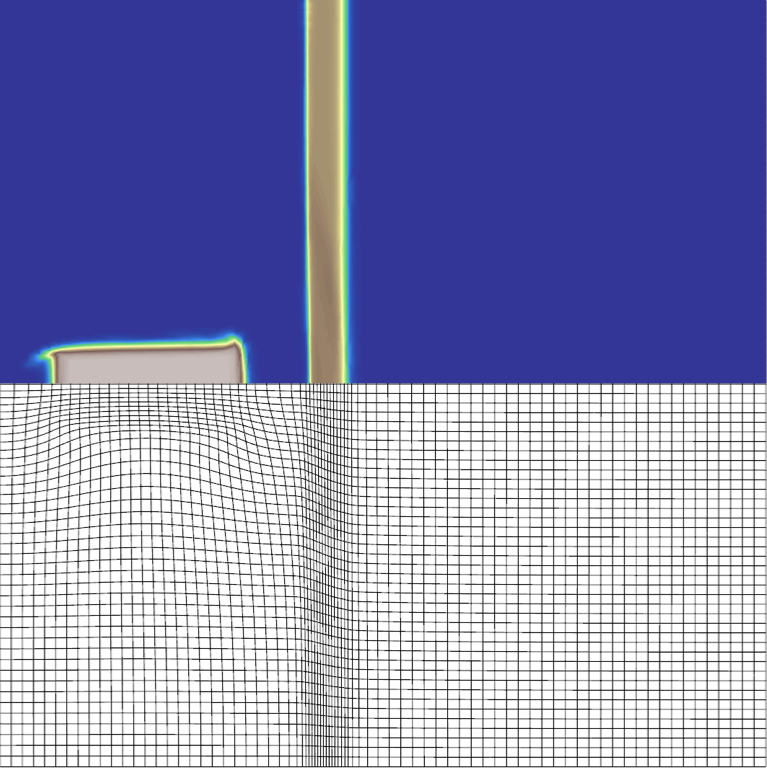
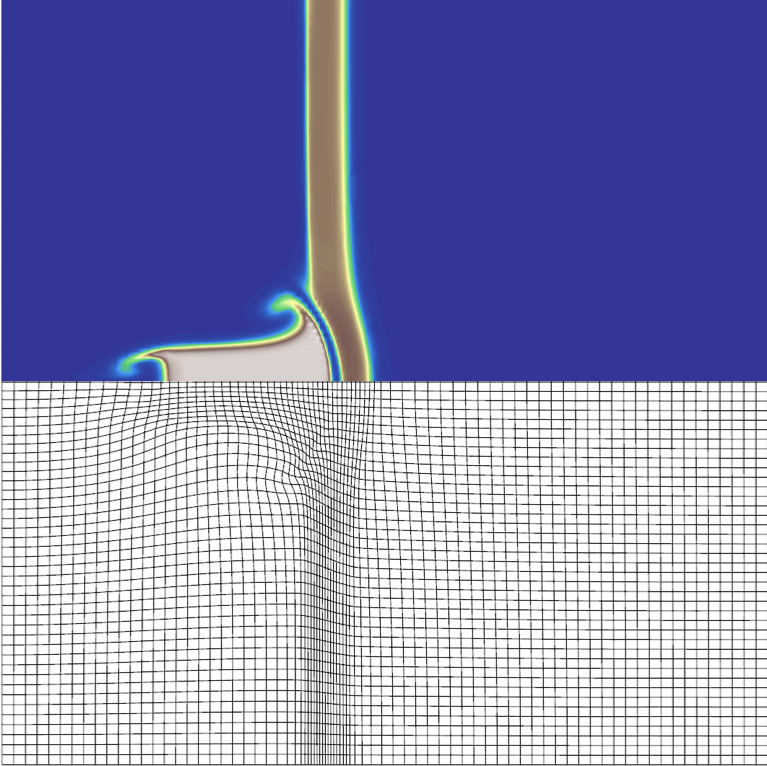
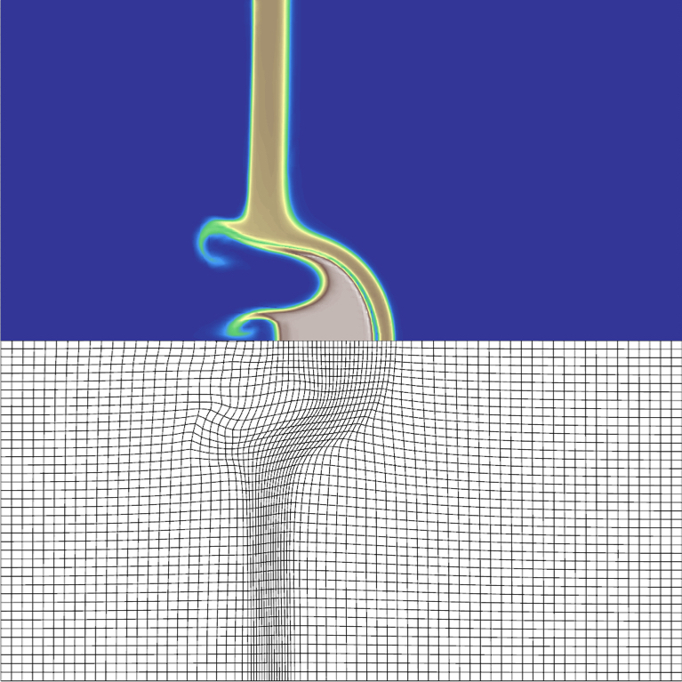
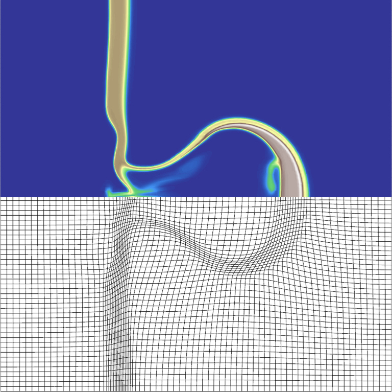
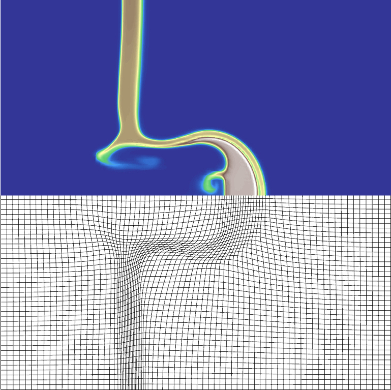
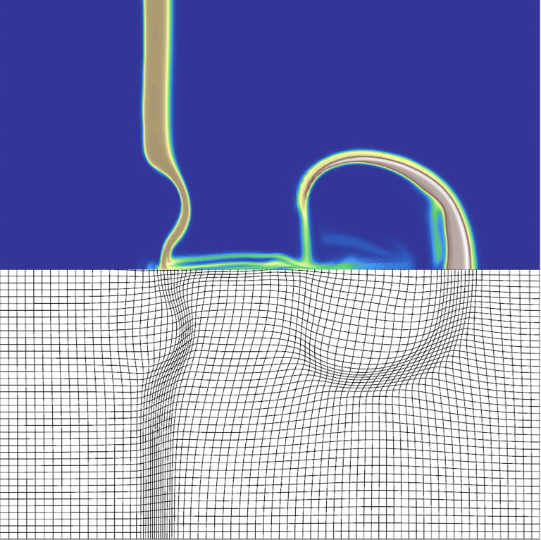
Figure 9: Time evolution of density and mesh position at times 0.5 (top left), 2 (top middle), 4 (top right), 6 (bottom left), 8 (bottom middle) and 10 (bottom right) in the 2D gas impact test case.

5.3 2Drz and 3D Full ALE Simulation of Steel Ball Impact on Unstructured Mesh

As a final example, we consider both 2Drz and full 3D calculations of a high velocity impact of a steel ball against an aluminum plate as described in [38, 13]. The problem consists of a spherical steel projectile of radius $5.5$ and initial velocity in the z-direction of $0.31cm/\mu s$ impacting a cylindrical plate of aluminum with a radius of $24$ and a thickness of $2.5$. Both the steel and aluminum materials use a Gruneisen equation of state combined with an elastic perfectly plastic “strength” model as described in [39]. This test demonstrates the ability of the method to adapt 2D and 3D unstructured meshes in the context of a practical ALE impact simulation.

In Figure 10 we show results of the 2D (axisymmetric) simulation on a sequence of refined 2D, high-order, unstructured meshes. Similarly to the previous example, we adapt to the position of the ball impactor, the aluminum plate, and all material interfaces, using the shape+size metric $\mu_{7}$. The adapted trigger is setup with $S_{22}=5$ in (10). For the sequence of mesh refinements, the calculations required a total of $3201$, $4815$ and $10145$ Lagrange time steps for the coarse, medium and fine meshes, respectively, to reach a final simulation time of $t=80$. The total number of remesh steps performed for the each 2Drz calculation is $19$, $39$ and $88$ for the coarse, medium and fine meshes, respectively. The total number of remap advection steps is $190$, $382$ and $782$.

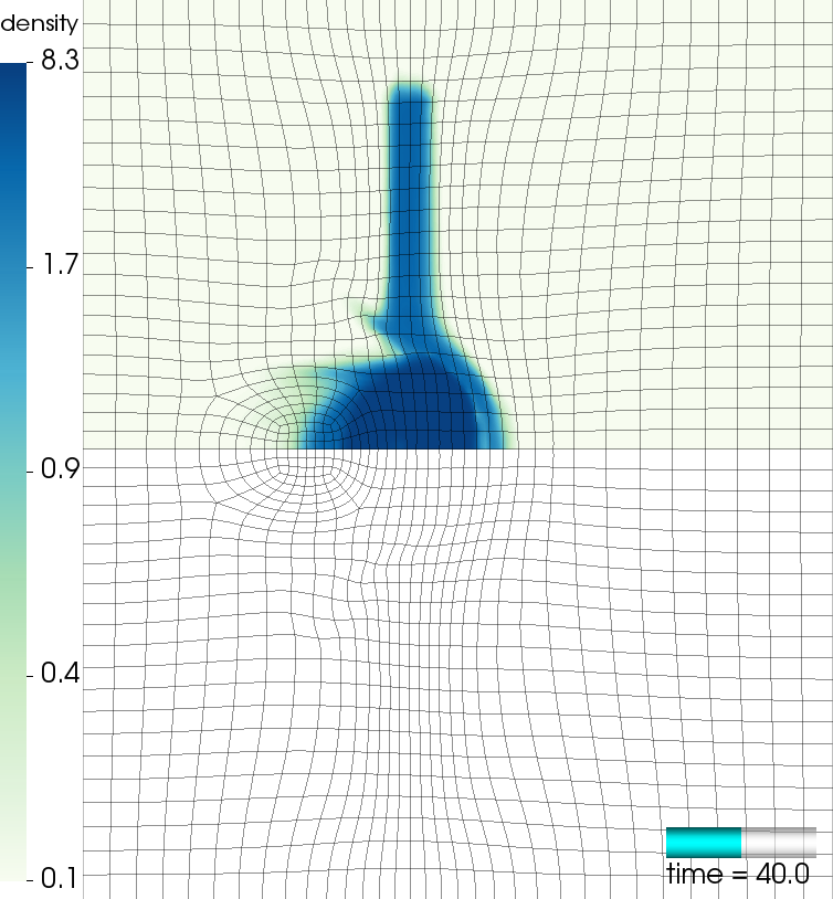
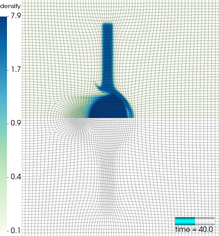
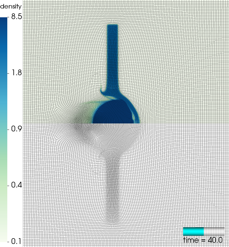
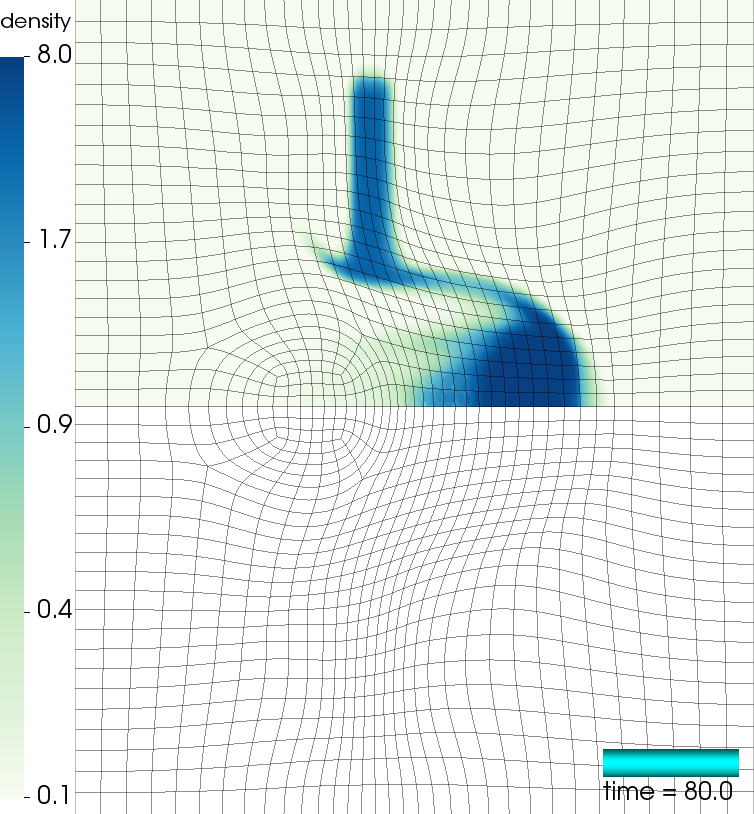
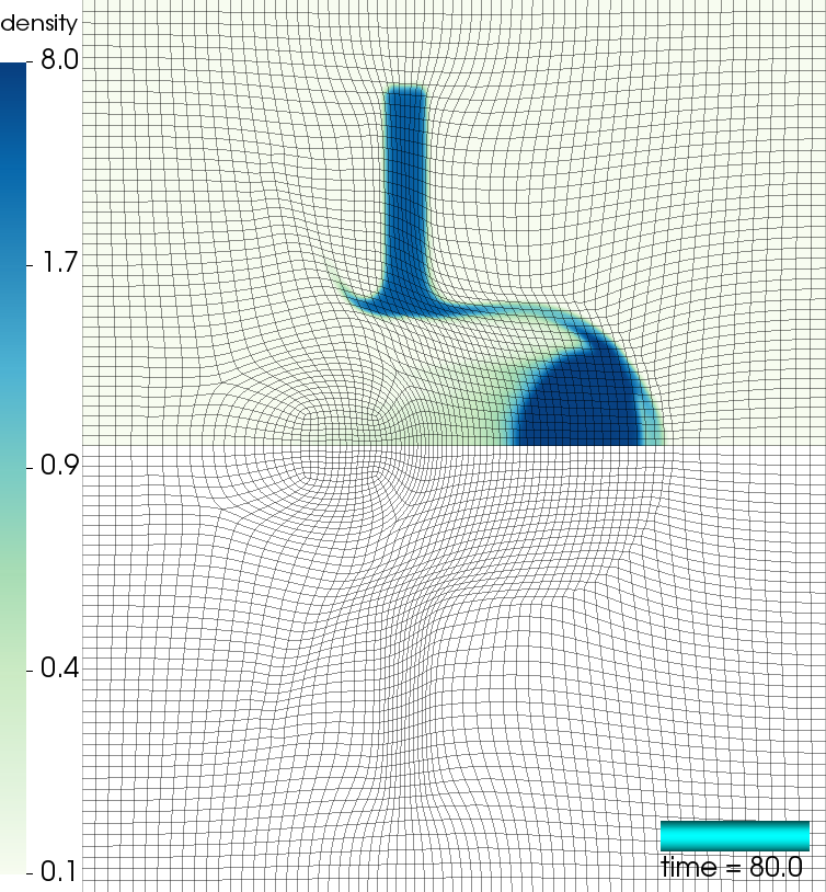
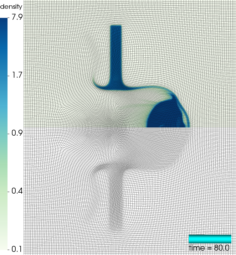
Figure 10: Density and mesh positions at times $t=40$ (top) and $t=80$ (bottom) using three different mesh resolutions for the 2Drz ball impact problem.

In Figure 11 we show results of the full 3D simulation on a high-order 3D unstructured mesh with resolution identical to the previous 2D medium case in $rz$ plane. The adaptivity parameters for this calculation are $\alpha=12$ and $S_{33}=8$ for the 3D version of (10). This calculation requires a total of $9671$ Lagrange time steps, $33$ remesh steps, and $817$ advection remap steps to reach a final simulation time of $t=80$.

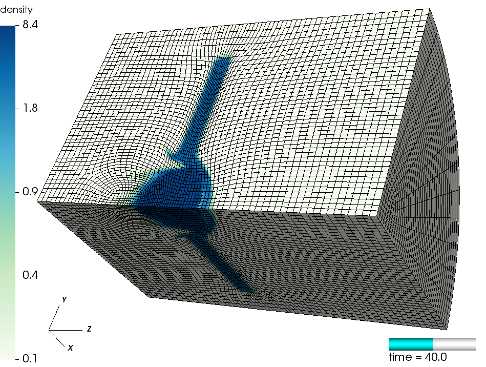
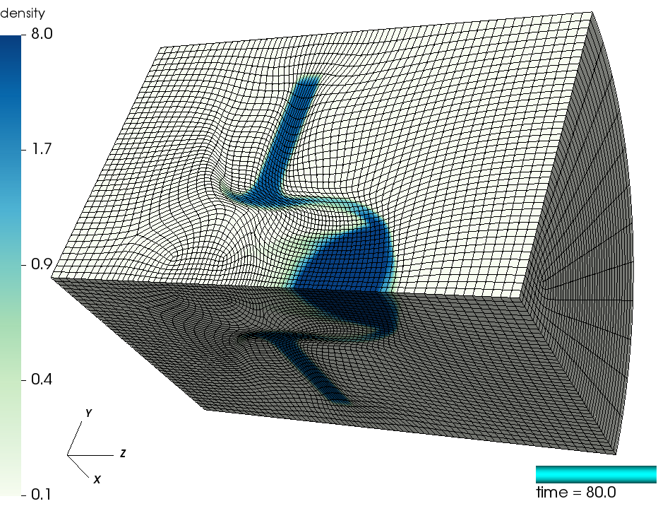
Figure 11: Density and mesh positions at times $t=40$ (left) and $t=80$ (right) for the 3D ball impact problem.

6 Conclusion

In this paper we have presented algorithms for simulation-driven optimization of high-order curved meshes, with application to high-order arbitrary Lagrangian-Eulerian simulations [2]. These allow the user to optimize the shape and size of the mesh, preserve geometric features, adapt the mesh characteristics to discrete fields of interest, and control the ALE frequency by adaptive triggers. These methods provide flexible control over the balance between computational time and amount of numerical dissipation in ALE simulations.

A future area of research will be to combine the existing TMOP technology with adaptive mesh refinement. This would allow to optimize shape, while achieving arbitrary small local size, which is currently constrained by the fact that the mesh topology is fixed. We also plan to add capabilities for tangential relaxation around discrete surfaces, which would be highly beneficial in multi-material ALE simulations.

In memoriam

This paper is dedicated to the memory of Dr. Douglas Nelson Woods (^∗January 11^th 1985 - $\dagger$September 11^th 2019), promising young scientist and post-doctoral research fellow at Los Alamos National Laboratory. Our thoughts and wishes go to his wife Jessica, to his parents Susan and Tom, to his sister Rebecca and to his brother Chris, whom he left behind.

Disclaimer

This document was prepared as an account of work sponsored by an agency of the United States government. Neither the United States government nor Lawrence Livermore National Security, LLC, nor any of their employees makes any warranty, expressed or implied, or assumes any legal liability or responsibility for the accuracy, completeness, or usefulness of any information, apparatus, product, or process disclosed, or represents that its use would not infringe privately owned rights. Reference herein to any specific commercial product, process, or service by trade name, trademark, manufacturer, or otherwise does not necessarily constitute or imply its endorsement, recommendation, or favoring by the United States government or Lawrence Livermore National Security, LLC. The views and opinions of authors expressed herein do not necessarily state or reflect those of the United States government or Lawrence Livermore National Security, LLC, and shall not be used for advertising or product endorsement purposes.

References

- [1] P. Knupp, Introducing the target-matrix paradigm for mesh optimization by node movement, Engr. with Comptr. 28 (4) (2012) 419–429.
- [2] BLAST: High-order finite element Lagrangian hydrocode, www.llnl.gov/CASC/blast.
- [3] J. V. Neumann, R. Richtmyer, A method for the numerical calculation of hydrodynamic shocks, J. Appl. Phys. 21 (1950).
- [4] D. J. Benson, Computational methods in Lagrangian and Eulerian hydrocodes, Comput. Methods Appl. Mech. Eng. 99 (1992) 235–394.
- [5] R. Loubere, J. Ovadia, R. Abgrall, A Lagrangian discontinuous Galerkin-type method on unstructured meshes to solve hydrodynamics problems, Int J. Num. Meth. Fluids 44 (2004) 645–663.
- [6] G. Scovazzi, M. Christon, T. Hughes, J. Shadid, Stabilized shock hydrodynamics: I. a Lagrangian method, Comp. Methods in Applied Mech. Eng. 196 (2007) 923–966.
- [7] P.-H. Maire, A high-order cell-centered Lagrangian scheme for two-dimensional compressible fluid flows on unstructured meshes, J. Comput. Phys. 228 (7) (2009) 2931–2425.
- [8] C. W. Hirt, A. A. Amsden, J. L. Cook, An arbitrary Lagrangian-Eulerian computing method for all flow speeds, J. Comput. Phys. 14 (1974) 277–253.
- [9] A. J. Barlow, P.-H. Maire, W. J. Rider, R. N. Rieben, M. J. Shashkov, Arbitrary Lagrangian-Eulerian methods for modeling high-speed compressible multimaterial flows, J. Comput. Phys. 322 (2016) 603–665.
- [10] P.-H. Maire, J. Breil, S. Galera, A cell-centred arbitrary Lagrangian–Eulerian (ALE) method, Int J. Num. Meth. Fluids 56 (2004) 1161–1166.
- [11] S. Galera, P.-H. Maire, J. Breil, A two-dimensional unstructured cell-centered multi-material ALE scheme using VOF interface reconstruction, J. Comput. Phys. 229 (16) (2010) 5755–5787.
- [12] V. Dobrev, T. Kolev, R. Rieben, High-order curvilinear finite element methods for Lagrangian hydrodynamics, SIAM J. Sci. Comp. 34 (5) (2012) 606–641.
- [13] V. A. Dobrev, T. V. Kolev, R. N. Rieben, V. Z. Tomov, Multi-material closure model for high-order finite element Lagrangian hydrodynamics, Int. J. Numer. Meth. Fluids 82 (10) (2016) 689–706.
- [14] R. W. Anderson, V. A. Dobrev, T. V. Kolev, R. N. Rieben, V. Z. Tomov, High-order multi-material ALE hydrodynamics, SIAM J. Sci. Comp. 40 (1) (2018) B32–B58.
- [15] V. A. Dobrev, P. Knupp, T. V. Kolev, K. Mittal, V. Z. Tomov, The Target-Matrix Optimization Paradigm for high-order meshes, SIAM J. Sci. Comp. 41 (1) (2019) B50–B68.
- [16] V. Dobrev, T. Ellis, T. Kolev, R. Rieben, High-order curvilinear finite elements for axisymmetric Lagrangian hydrodynamics, Computers & Fluids (2013) 58–69.
- [17] J.-L. Guermond, B. Popov, V. Tomov, Entropy-viscosity method for the single material Euler equations in Lagrangian frame, Computer Methods in Applied Mechanics and Engineering 300 (2016) 402 – 426.
- [18] W. Boscheri, M. Dumbser, High order accurate direct arbitrary-Lagrangian-Eulerian ADER-WENO finite volume schemes on moving curvilinear unstructured meshes, Computers & Fluids 136 (2016) 48 – 66.
- [19] X. Zeng, G. Scovazzi, A variational multiscale finite element method for monolithic ALE computations of shock hydrodynamics using nodal elements, J. Comput. Phys. 315 (2016) 577–608.
- [20] J. Bakosi, J. Waltz, N. Morgan, Improved ALE mesh velocities for complex flows, Int J. Num. Meth. Fluids 85 (11) (2017) 662–671.
- [21] E. Gaburro, M. Dumbser, M. Castro, Direct Arbitrary-Lagrangian-Eulerian finite volume schemes on moving nonconforming unstructured meshes, Computers and Fluids 159 (15) (2017) 254–275.
- [22] M. Kucharik, R. Garimella, S. Schofield, M. Shashkov, A comparative study of interface reconstruction methods for multi‐material ALE simulations, J. Comput. Phys. 229 (7) (2010) 2432–2452.
- [23] R. Loubère, P.-H. Maire, M. Shashkov, J. Breil, S. Galera, ReALE: A reconnection-based arbitrary-Lagrangian–Eulerian method, J. Comput. Phys. 229 (12) (2010) 4724–4761.
- [24] V. A. Dobrev, P. Knupp, T. V. Kolev, V. Z. Tomov, Towards Simulation-Driven Optimization of High-Order Meshes by the Target-Matrix Optimization Paradigm, Springer International Publishing, 2019, pp. 285–302.
- [25] P. Knupp, Target formulation and construction in mesh quality improvement, Tech. Rep. LLNL-TR-795097, Lawrence Livermore National Lab.(LLNL), Livermore, CA (United States) (2019).
- [26] K. Mittal, P. Fischer, Mesh smoothing for the spectral element method, Journal of Scientific Computing 78 (2) (2019) 1152–1173.
- [27] V. Garanzha, L. Kudryavtseva, S. Utyuzhnikov, Variational method for untangling and optimization of spatial meshes, J. Comput. Appl. Math. 269 (2014) 24–41.
- [28] V. A. Garanzha, Polyconvex potentials, invertible deformations, and thermodynamically consistent formulation of the nonlinear elasticity equations, Comp. Math. Math. Phys. 50 (9) (2010) 1561–1587.
- [29] W. Huang, R. D. Russell, Adaptive moving mesh methods, Springer Science & Business Media, 2010.
- [30] P. T. Greene, S. P. Schofield, R. Nourgaliev, Dynamic mesh adaptation for front evolution using discontinuous Galerkin based weighted condition number relaxation, Journal of Computational Physics 335 (2017) 664–687.
- [31] P. Váchal, P.-H. Maire, Discretizations for weighted condition number smoothing on general unstructured meshes, Computers & Fluids 46 (1) (2011) 479 – 485.
- [32] G. Aparicio-Estrems, A. Gargallo-Peiró, X. Roca, Defining a stretching and alignment aware quality measure for linear and curved 2D meshes, Springer International Publishing, 2019, pp. 37–55.
- [33] J. Marcon, G. Castiglioni, D. Moxey, S. J. Sherwin, J. Peiró, -adaptation for compressible flows, arXiv preprint arXiv:1909.10973 (2019).
- [34] K. Mittal, S. Dutta, P. Fischer, Nonconforming schwarz-spectral element methods for incompressible flow, Computers & Fluids 191 (2019) 104237.
- [35] MFEM: Modular finite element methods library, mfem.org. doi:10.11578/dc.20171025.1248.
- [36] R. Anderson, J. Andrej, A. Barker, J. Bramwell, J.-S. Camier, J. Cerveny, V. Dobrev, Y. Dudouit, A. Fisher, T. Kolev, W. Pazner, M. Stowell, V. Tomov, J. Dahm, D. Medina, S. Zampini, MFEM: A modular finite element methods library, in review (2019). arXiv:1911.09220.
- [37] A. Barlow, R. Hill, M. J. Shashkov, Constrained optimization framework for interface-aware sub-scale dynamics closure model for multimaterial cells in Lagrangian and arbitrary Lagrangian-Eulerian hydrodynamics, J. Comput. Phys. 276 (0) (2014) 92–135.
- [38] B. P. Howell, G. J. Ball, A free-Lagrange augmented Godunov method for the simulation of elastic-plastic solids, J. Comput. Phys. 175 (2002) 128–167.
- [39] V. A. Dobrev, T. V. Kolev, R. N. Rieben, High-order curvilinear finite elements for elastic-plastic Lagrangian dynamics, Journal of Computational Physics 257 (B) (2014) 1062–1080.