Nucleon Axial Form Factors from Clover Fermion on $2+1+1$-flavor HISQ Lattice

Abstract:

The nucleon axial form factors – axial $G_{A}$, induced pseudoscalar $\widetilde{G}_{P}$ and pseudoscalar $G_{P}$ – have displayed large systematics in lattice QCD calculations. The major symptoms were the violation of the partially conserved axial current (PCAC) relation between the three form factors, and the underestimation of the induced pseudoscalar coupling $g_{P}^{\ast}$ and the axial charge radius $r_{A}$ compared to phenomenological estimates. The small $g_{P}^{\ast}$ was a consequence of the failure of the pion-pole dominance (PPD) hypothesis, especially at low $M_{\pi}^{2}$. The small charge radius $r_{A}$ and the underestimate of $g_{A}$ were related. The dominant systematic responsible is the lack of inclusion of low-energy ($N\pi$) states that are not manifest in the multiexponential fit to the nucleon two-point correlator. We show that this low-energy state can be determined from the three-point correlator $\langle NA_{4}N\rangle$ with the insertion of the temporal component of the axial current $A_{4}$ within the nucleon state, ie, the strategy labeled $S_{A4}$ [1]. Including this low-energy state in fits to control excited-state contamination (ESC) gives results for $g_{A}$, $r_{A}$, and $g_{P}^{\ast}$ that are consistent with experimental/phenomenological values. However, the systematic uncertainties, especially in data at small $Q^{2}$, are now much larger.

1 Introduction

Nucleon matrix elements of the axial $A_{\mu}=\bar{u}\gamma_{\mu}\gamma_{5}d$ and pseudoscalar $P=\bar{u}\gamma_{5}d$ currents can be decomposed into the axial $G_{A}$, induced pseudoscalar $\widetilde{G}_{P}$, and pseudoscalar $G_{P}$ form factors as

$$\langle N(\vec{p}_{f})\lvert A_{\mu}(\vec{Q})\rvert N(\vec{p}_{i})\rangle ={\overline{u}}(\vec{p}_{f})\left[G_{A}(Q^{2})\gamma_{\mu}+q_{\mu}\frac{\widetilde{G}_{P}(Q^{2})}{2M}\right]\gamma_{5}u(\vec{p}_{i})\,,$$ (1)

$$\langle N(\vec{p}_{f})\lvert P(\vec{q})\rvert N(\vec{p}_{i})\rangle ={\overline{u}}(\vec{p}_{f})\left[G_{P}(Q^{2})\gamma_{5}\right]u(\vec{p}_{i})\,,$$ (2)

where $q=p_{f}-p_{i}$, and the initial nucleon is at rest $\vec{p}_{i}=0$ in our lattice calculation. The space-like four momentum transfer $Q^{2}(=-q^{2})=\vec{p}_{f}^{2}-(E(\vec{p}_{f})-M)^{2}$. Note that we work in the isospin limit, $m_{u}=m_{d}$, and present results only for the isovector currents, e.g., $A_{\mu}^{u-d}=\bar{u}\gamma_{\mu}\gamma_{5}u-\bar{d}\gamma_{\mu}\gamma_{5}d$ so that $\langle p\lvert A_{\mu}\rvert n\rangle=\langle p\lvert A_{\mu}^{u-d}\rvert p\rangle$. The axial charge $g_{A}$ and charge radius $r_{A}$ are defined at zero-momentum transfer $Q^{2}=0$: $G_{A}(0)\equiv g_{A}$ and $\langle r_{A}^{2}\rangle=-6\frac{d}{dQ^{2}}\left.\left(\frac{G_{A}(Q^{2})}{G_{A}(0)}\right)\right|_{Q^{2}=0}$.

The lattice axial form factor $G_{A}$ has traditionally been extracted by fitting the spectral decomposition of the 3-point functions using the spectrum taken from fits to 2-point functions (called the standard strategy $S_{\text{2pt}}$ hereafter). These data have shown significant violation of the PCAC relation,

$$\text{PCAC}:\;2{\widehat{m}}G_{P}(Q^{2}) =2MG_{A}(Q^{2})-\frac{Q^{2}}{2M}{\widetilde{G}}_{P}(Q^{2})\,,\quad\text{PPD}:\;\widetilde{G}_{P}(Q^{2})=\frac{4M^{2}}{Q^{2}+M_{\pi}^{2}}G_{A}(Q^{2})\,,$$ (3)

among the three form factors [2], as shown in the top left panel of Fig. 1. Here $\hat{m}$ is the PCAC quark mass. Analogously, the induced pseudoscalar form factor $\widetilde{G}_{P}$ with $S_{\text{2pt}}$ does not follow the $M_{\pi}^{2}$ behavior predicted by pion-pole dominance (PPD) (Fig. 1 bottom left panel), and gives a smaller $g_{P}^{\ast}\sim 0.6g_{P}^{\ast}|_{\text{exp}}$ than the experimental value (Fig. 5 left panel). Fits to the axial form factor give a much larger axial mass than obtained from a phenomenological parameterization of neutrino-nucleus scattering data as shown in Fig. 2 left panel. These deviations in $G_{A}$ result in a $g_{A}$ that is smaller than the experimental value $g_{A}=1.2766(20)$, and also a smaller charge radius $r_{A}$.

In Ref. [1], we showed that $S_{\text{2pt}}$ does not include a lower energy excited state that dominates the 3-point correlator with the insertion of $A_{4}$. This correlator, $C_{A4}^{\text{3pt}}$, had been neglected in previous analyses because of the large ESC and the failure of $S_{\text{2pt}}$ to fit it. We show that the large contribution of excited-states to $C_{A4}^{\text{3pt}}$ allows us to isolate a “state” with energy close to the noninteracting $N(\vec{0})\pi(\vec{p})$ state (or $N(-\vec{p})\pi(\vec{p})$ depending on the momentum combinations). The new strategy, $S_{A4}$ with excited state energy from the $C_{A4}^{\text{3pt}}$ and ground state mass $M$ and energy $E(\vec{p})$ from the two-point correlators, fixes PCAC and gives $g_{P}^{\ast}\approx g_{P}^{\ast}|_{\text{exp}}$. This was demonstrated using the physical pion mass ensemble $a09m130W$ in Ref. [1] and discussed in Section 2.

In the following sections, we present a comparison of the axial form factors extracted from the two strategies, $S_{\text{2pt}}$ and $S_{A4}$ [1] for 13 calculations on 11 ensembles of $2+1+1$-flavor HISQ lattice generated by the MILC collaboration [3]. Details of the lattice parameters, statistics accumulated and the spectrum used in the strategy $S_{\text{2pt}}$ can be found in Ref. [4]. 

2 PCAC and Pion-pole Dominance (PPD)

Tests of the PCAC relation and PPD hypothesis given in Eq. (3) are shown in Fig. 1 in term of the ratios $R_{1}+R_{2}$ and $R_{3}$ with

$$R_{1}= \;\frac{Q^{2}}{4M^{2}}\frac{{\tilde{G}}_{P}(Q^{2})}{G_{A}(Q^{2})}\,,\quad R_{2}=\frac{2{\widehat{m}}}{2M}\frac{G_{P}(Q^{2})}{G_{A}(Q^{2})}\,,\quad R_{3}=\frac{Q^{2}+M_{\pi}^{2}}{4M^{2}}\frac{{\tilde{G}}_{P}(Q^{2})}{G_{A}(Q^{2})}\,.$$ (4)

The left panels show increasing violation of PCAC and PPD with $S_{\text{2pt}}$ as $Q^{2}\to 0$, $M_{\pi}\to 135\,\mathrm{MeV}$ and $a\to 0$, ie, deviation from unity. This violation is reduced to $\lesssim 5\%$ with $S_{A4}$ as shown in the right panels. Once PPD is demonstrated, the improvement in the continuum limit result for the induced pseudoscalar coupling $g_{P}^{\ast}$ follows as a consequence as discussed in Sec. 4.

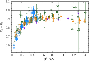
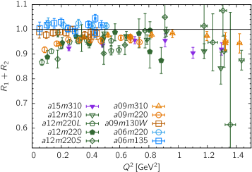
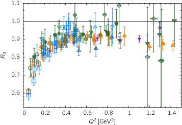
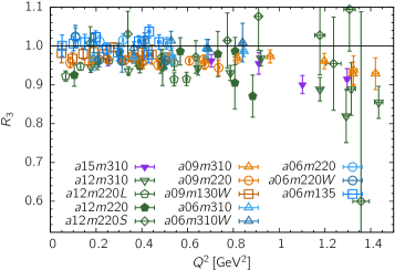
Figure 1: Tests of the PCAC relation $R_{1}+R_{2}=1$ and the PPD $R_{3}=1$ for (left) $S_{\text{2pt}}$ and (right) $S_{A4}$.

3 Axial Form Factor $G_{A}$

In Fig. 2, the axial form factor $G_{A}$ from two strategies $S_{\text{2pt}}$ and $S_{A4}$ are compared. The lattice data for $G_{A}$ from $S_{\text{2pt}}$ are systematically above the phenomenological curve (dipole fit with $M_{A}=1.026(21)$ GeV) for the available kinematic range $0<Q^{2}\lesssim 1.4\,\mathrm{GeV}^{2}$, while variations in lattice spacing and pion mass are smaller than the deviation from that curve. Compared to Refs. [5, 6, 2], the increased statistics, number of data sets ($8\to 13$), and the number of excited states included in the three-point correlator fits ($2\to 3^{\ast}$) do not result in a significant change in the data or the overall picture, and the deviation persists. The spread with the strategy $S_{A4}$ is larger as shown in Fig. 2 (right). Note that different $g_{A}$ are used to normalize $G_{A}(Q^{2}\neq 0)$ in the two panels in Fig. 2: $g_{A}$ from a direct fit to $C_{A3}^{\text{3pt}}(\vec{p}=\vec{0})$ when using $S_{\text{2pt}}$, and extrapolation of the z-expansion fit to the nonzero momentum transfer data obtained with $S_{A4}$.

While one can extract $g_{A}$ from a direct fit to $C_{A3}^{\text{3pt}}(\vec{p}=\vec{0})$ with $S_{\text{2pt}}$ but, because the $A_{4}$ correlator vanishes at zero momentum, there is no information on the relevant excited states with $S_{A4}$ from the $A_{4}$ channel. Thus, within $S_{A4}$ it is not obvious what value of $g_{A}$ to use to plot $G_{A}(Q^{2})/g_{A}$. One can determine $g_{A}$ by extrapolating the $G_{A}(Q^{2}\neq 0)$ data using the z-expansion or the dipole ansatz. We find that these estimates have a larger uncertainty and the dipole ansatz does not fit the small $Q^{2}$ data with $S_{A4}$ in most cases. One can also extract it by assuming that $N(\bm{p}=1)\pi(\bm{p}=-1)$ is the relevant lightest excited state or by leaving the first excited state energy a free parameter in the fits used to remove ESC. Note that when using these alternate methods for $g_{A}$ with $S_{A4}$, the renormalized form factor $G_{A}/g_{A}$ can [under]overshoot the expected value 1.0 at $Q^{2}=0$. Also, the difference in $G_{A}(Q^{2})$ between $S_{\text{2pt}}$ and $S_{A4}$ is mainly manifest at the smallest $Q^{2}$ on the physical mass ensembles. Thus, it is important to control this systematic, and we are still exploring options to get reliable estimates and defensible uncertainty quantification in them.

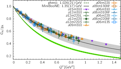
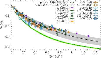
Figure 2: Comparing the axial form factor $G_{A}$ with charge $g_{A}$ extracted using strategy $S_{\text{2pt}}$ (left) with $G_{A}$ from strategy $S_{A4}$ and normalized by $g_{A}$ obtained from a $z^{2}$-fit ($z^{1}$-fit for the two physical ensemble) to it.

Preliminary results for the axial charge $g_{A}$ and $r_{A}^{2}$ obtained using the $z$-expansion fits are shown in Fig. 3 along with the continuum-chiral-finite-volume (CCFV) fits to get their values at $a\to 0$, $M_{\pi}L\to\infty$ and $M_{\pi}=135\,\mathrm{MeV}$. In the fits, we imposed the bound $\lvert a_{i}\rvert\leq 5$ on the $z$-expansion coefficients by using gaussian priors to stabilize higher order fits and applied a cutoff $Q^{2}_{\text{cut}}\sim 1$ GeV, above which the extraction of the data are not yet reliable. Overall, the $z^{k}$-expansion fits with order $k=1$ and $k=2$ describe the data well, and the changes in $g_{A}$ and $r_{A}^{2}$ with $k\geq 2$ are small. Results from the CCFV fits are given in Table 1. At present, the crucial $a06m135$ physical mass ensemble data have large errors, so we are working to increase the statistics and thereby improve the reliability of the CCFV fits.

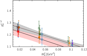
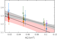
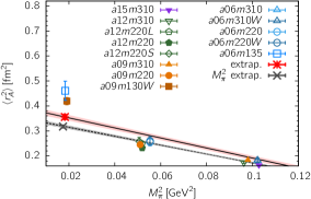
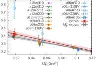
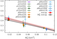
Figure 3: Data and CCFV fits (the pink band with the black solid line) using the ansatz $y=b_{0}+b_{1}a+b_{2}M_{\pi}^{2}+b_{3}M_{\pi}^{2}\exp(-M_{\pi}L)$ for $g_{A}$ (top) and $r_{A}^{2}$ (bottom). On each ensemble, $g_{A}$ and $r_{A}^{2}$ are obtained using the $z$-expansion with order $k=1$ (left), $k=2$ (middle), and $k=1$ for the two physical mass ensembles and $k=2$ for the rest (right). The grey band with the black dashed line is a fit with $b_{1}=b_{3}=0$. Result of the extrapolation are given in Table 1.

Ref.	$g_{A}$	$\chi^{2}/\text{dof}$	$p$-value	$\langle r_{A}^{2}\rangle\,[\mathrm{fm}^{2}]$	$\chi^{2}/\text{dof}$	$p$-value
Fig. 3, left	1.23(4)	0.19	0.99	0.356(10)	7.64	3$\times 10^{-11}$
Fig. 3, middle	1.28(5)	0.34	0.96	0.428(31)	1.90	0.05
Fig. 3, right	1.24(5)	0.37	0.95	0.444(22)	1.34	0.21

Table 1: Results for $g_{A}$ and $r_{A}^{2}$ from the CCFV fits shown in Fig. 3.

4 Induced Pseudoscalar $\widetilde{G}_{P}$ and Pseudoscalar $G_{P}$ Form Factors

Data for the induced pseudoscalar $\widetilde{G}_{P}$ and pseudoscalar $G_{P}$ form factors from two strategies $S_{\text{2pt}}$ and $S_{A4}$ are summarized in Fig. 4. Both form factors, and consequently the induced pseudoscalar coupling $g_{P}^{\ast}\equiv(m_{\mu}/2M)\widetilde{G}_{P}(0.88m_{\mu}^{3})$, are clearly enhanced at the small $Q^{2}$ with $S_{A4}$. Note that we do not have data for $G_{P}$ on the three ensembles $a06m310$, $a06m310W$, $a06m220W$.

To extract $g_{P}^{\ast}$ on each ensemble, we fit $\widetilde{G}_{P}$ using Eq. (5) and read off the value at the kinematic point $Q^{2}=0.88m_{\mu}^{2}$. Eq. (5) includes the pion-pole and the leading analytical behavior.

$$\tilde{G}_{P}(Q^{2})= \;\frac{c_{0}}{Q^{2}+M_{\pi}^{2}}+c_{1}+c_{2}Q^{2}\,.$$ (5)

$$Y_{1,2}(a,M_{\pi}){}= \;\frac{d_{1}}{M_{\pi}^{2}+0.88m_{\mu}^{2}}+d_{2}+d_{3}a+d_{4}M_{\pi}^{2}\,.$$ (6)

Result at the physical point, $a\to 0$ and $M_{\pi}=135\,\mathrm{MeV}$, is obtained using Eq. (6) with the data renormalized using two different methods: $Y_{1}=g_{P}^{\ast}/g_{A}=g_{P}^{\ast\;\text{(bare)}}/g_{A}^{\text{(bare)}}$ and $Y_{2}=g_{P}^{\ast}=Z_{A}g_{P}^{\ast\;\text{(bare)}}$. The $g_{P}^{\ast}$ with strategy $S_{A4}$ is consistent with the experimental value $g_{P}^{\ast}|_{\text{MuCap}}=8.06(55)$ [7, 8] obtained from the MuCap experiment $[\mu^{-}+p\to\nu_{\mu}+n]$, or $g_{P}^{\ast}/g_{A}|_{\text{MuCap}}=6.31(70)$ with $g_{A}|_{\text{exp}}=1.2766(20)$.

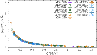
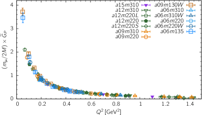
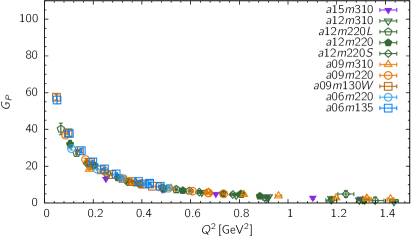
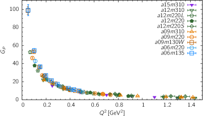
Figure 4: Comparison of $(m_{\mu}/2M)\times\widetilde{G}_{P}$ (top) and $G_{P}$ (bottom) obtained using the two strategies $S_{\text{2pt}}$ (left) and $S_{A4}$ (right). Here, the form factors are not renormalized.

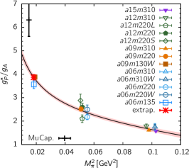
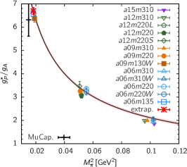
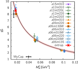
Figure 5: Chrial continuum fit using Eq. (6) to $g_{P}^{\ast}/g_{A}=g_{P}^{\ast\;\text{(bare)}}/g_{A}^{\text{(bare)}}$ data with $S_{\text{2pt}}$ (left) and $S_{A4}$ with $g_{A}$ from the $z^{2}$-fit to $G_{A}(Q^{2}\neq 0)$ data (middle). (right) $g_{P}^{\ast}=Z_{A}g_{P}^{\ast\;\text{(bare)}}$, where $g_{P}^{\ast\;\text{(bare)}}$ data are the same as in the middle panel and $Z_{A}$ is the axial current renormalization factor that is calculated independently [9].

Ref.	$g_{P}^{\ast}/g_{A}$	$d_{1}\;[\mathrm{GeV}^{2}]$	$d_{2}$	$d_{3}\;[\mathrm{fm}^{-1}]$	$d_{4}\;[\mathrm{GeV}^{-2}]$	$\chi^{2}/\text{dof}$	$p$-value
Fig. 5, left	3.87(11)	0.056(09)	1.91(31)	-0.08(70)	-8.0(2.5)	2.27	0.02
Fig. 5, middle	6.69(14)	0.159(09)	0.78(27)	-1.66(55)	-1.4(1.8)	1.27	0.24
Ref.	$g_{P}^{\ast}$	$d_{1}\;[\mathrm{GeV}^{2}]$	$d_{2}$	$d_{3}\;[\mathrm{fm}^{-1}]$	$d_{4}\;[\mathrm{GeV}^{-2}]$	$\chi^{2}/\text{dof}$	$p$-value
Fig. 5, right	8.60(39)	0.208(26)	0.94(73)	-1.11(1.33)	-4.0(5.1)	0.91	0.51

Table 2: Results for the chiral-continuum extrapolation of $g_{P}^{\ast}/g_{A}$ and $g_{P}^{\ast}$ using Eq. (6).

5 Summary

We present a comparison between two strategies, $S_{\text{2pt}}$ and $S_{A4}$, for extracting the nucleon isovector axial form factors, $G_{A}$, induced pseudoscalar $\widetilde{G}_{P}$, and pseudoscalar $G_{P}$. The new strategy $S_{A4}$ incorporates a low-energy state that was not exposed by multistate fits to nucleon two-point correlators constructed with a conventional nucleon interpolating operator. Incorporating these lower lying excited states largely impacts the pseudoscalar $G_{P}$ and induced pseudoscalar $\widetilde{G}_{P}$ form factors. As a result, the PCAC relation and PPD hypothesis are now resonably well satisfied: the deviation is reduced to about 10% for heavy pion mass ensembles and to only a few percent for the physical mass ensembles. Consequently, the induced pseudoscalar coupling $g_{P}^{\ast}$ is also consistent with the experimental value.

The axial form factor $G_{A}$ shows a much smaller shift compared to $G_{P}$ and $\widetilde{G}_{P}$ that is evident only at the smallest $Q^{2}$. Unfortunately, becasue of the kinematic constraint, one cannot extract $g_{A}$ (the data point at $Q^{2}=0$) with strategy $S_{A4}$. The small $Q^{2}$ behavior is also critical for determining the axial charge radius $r_{A}$. At discussed in Sec. 3, analysis of the small $Q^{2}$ (and $Q^{2}=0$) behavior is under progress and the statistics on the $a06m135$ ensemble are being increased.

The new strategy $S_{A4}$ uses a 2-state fit for the three-point correlator analysis. While inclusion of a single “effective” lower energy excited state dramatically improves PCAC and PPD, it is essential to develop methods that will provide a more detailed and refined picture of the many possible excited states that can contribute. Including the full tower of states that provide significant ESC and controlling this systematics is necessary for precision calculations of the axial form factors.

References

- [1] Y.-C. Jang, R. Gupta, B. Yoon, and T. Bhattacharya, 1905.06470.
- [2] R. Gupta, Y.-C. Jang, H.-W. Lin, B. Yoon, and T. Bhattacharya, Phys. Rev. D96 (2017), no. 11 114503, [1705.06834].
- [3] A. Bazavov et al., Phys. Rev. D87 (2013), no. 5 054505, [1212.4768].
- [4] Y.-C. Jang, R. Gupta, H.-W. Lin, B. Yoon, and T. Bhattacharya, Phys. Rev. D101 (2020), no. 1 014507, [1906.07217].
- [5] Y.-C. Jang et al., EPJ Web Conf. 175 (2018) 06033, [1801.01635].
- [6] Y.-C. Jang et al., PoS LATTICE2018 (2018) 123, [1901.00060].
- [7] V. A. Andreev et al., MuCap, Phys. Rev. Lett. 110 (2013), no. 1 012504, [1210.6545].
- [8] V. A. Andreev et al., MuCap, Phys. Rev. C91 (2015), no. 5 055502, [1502.00913].
- [9] R. Gupta, Y.-C. Jang, B. Yoon, H.-W. Lin, V. Cirigliano, and T. Bhattacharya, Phys. Rev. D98 (2018) 034503, [1806.09006].
- [10] R. G. Edwards and B. Joo, Nucl.Phys.Proc.Suppl. 140 (2005) 832, [hep-lat/0409003].