Spatiotemporal chaos and quasipatterns in coupled reaction–diffusion systems

Abstract

In coupled reaction–diffusion systems, modes with two different length scales can interact to produce a wide variety of spatiotemporal patterns. Three-wave interactions between these modes can explain the occurrence of spatially complex steady patterns and time-varying states including spatiotemporal chaos. The interactions can take the form of two short waves with different orientations interacting with one long wave, or vice verse. We investigate the role of such three-wave interactions in a coupled Brusselator system. As well as finding simple steady patterns when the waves reinforce each other, we can also find spatially complex but steady patterns, including quasipatterns. When the waves compete with each other, time varying states such as spatiotemporal chaos are also possible. The signs of the quadratic coefficients in three-wave interaction equations distinguish between these two cases. By manipulating parameters of the chemical model, the formation of these various states can be encouraged, as we confirm through extensive numerical simulation. Our arguments allow us to predict when spatiotemporal chaos might be found: standard nonlinear methods fail in this case. The arguments are quite general and apply to a wide class of pattern-forming systems, including the Faraday wave experiment.

1 Introduction

Two substances that react and diffuse can form patterns, an insight first highlighted in the work of Alan Turing [1, 2]. Motivated by an interest in embryonic morphogenesis, Turing studied discrete and continuum models for the spontaneous emergence of structure in a ring of cells. Depending on the details of the reaction, a Turing-type system may have a stable, spatially-uniform steady state in the absence of diffusion. Two fundamental instabilities may occur. One possibility is a Hopf bifurcation leading to temporal oscillations with a preferred wavenumber of zero. The other possibility, driven by diffusion, is a bifurcation to a steady spatial pattern (Turing pattern) with non-zero wavenumber, typically stripes or hexagons.

The first laboratory experiment to produce a Turing pattern came nearly 40 years after Turing’s original work: Ref. [3] reports the observation of patterns in the chlorite–iodide–malonic acid (CIMA) chemical reaction. Since the seminal discoveries of [1, 3], there has been a vast literature on reaction–diffusion patterns and their applications, which include animal skin pigmentation [4], the cerebral cortex [5], vegetation ecology [6], plankton colonies [7], and many others [8, 9].

A variation on the classic reaction–diffusion system is the so-called coupled (or multilayered) system, in which two or more reaction–diffusion systems are connected together so that they may influence each other. Because of the additional degrees of freedom in these coupled systems, they are an amenable setting in which to investigate how competing instabilities affect pattern formation. Coupled systems can produce a variety of states including simple Turing patterns, standing waves, mixes of Turing patterns and spiral waves, square and hexagonal superlattice patterns, and many more [10, 11]. Coupled systems are important in biology, especially in neural, ecological and developmental contexts; see [12] for examples and for an overview of selected results.

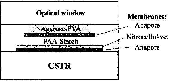
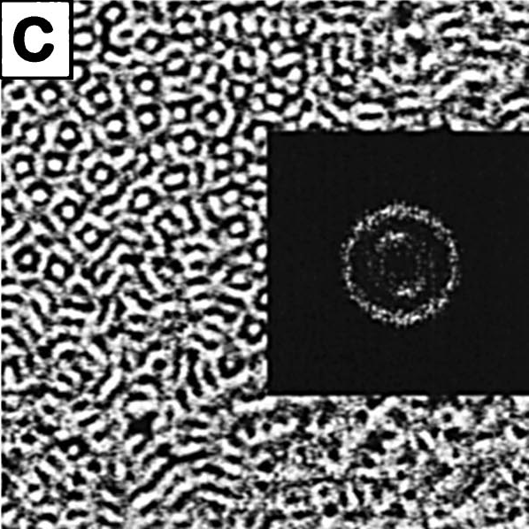
Figure 1: Patterns formed when the chlorine dioxide–iodine–malonic acid (CDIMA) reaction occurs in two layers that are diffusively coupled. Left: Experimental setup: the chemical reactions occur in the agarose–PVA and PAA–starch layers, separated by an Anapore membrane. Right: Patterns with two different length-scales ($0.46\,$mm and $0.25\,$mm) visualised through a filter transparent to red light (which highlights the pattern in the PAA–starch layer), with the corresponding spatial power spectrum in the inset. Reproduced from [13] with permission.

Unfortunately, it is difficult to manipulate experiments on the aforementioned biological systems. A common approach to studying coupled reaction–diffusion systems, then, is to study a paradigmatic chemical experiment in the laboratory, as in [13] (see Figure 1). In this work, the experimentalists set up two thin gels, within each of which the chlorine dioxide–iodine–malonic acid (CDIMA) reaction takes place. They put the gels in contact and controlled the strength of coupling between the two layers by modifying the properties of a membrane placed at the interface, resulting in different patterns. To complement laboratory experiments, investigators have studied a host of nonlinear partial differential equation (PDE) models, including the Lengyel–Epstein model of the CIMA reaction [14] and Brusselator model of a generic trimolecular reaction [15].

The work of [16] included a theoretical study of two reaction–diffusion systems coupled together in a parameter regime near a codimension-two Turing–Turing bifurcation point. This work demonstrated that by changing the interlayer coupling strength, one can manipulate the ratio of the length scales associated with two resonantly interacting Turing instabilities and encourage the formation of certain complex patterns in the Brusselator model. In our present work, we will also carry out a theoretical investigation of coupled reaction–diffusion systems and we will also focus on resonant mode interactions. However, in contrast to the set-up in [16], we will use the within-layer diffusion constants as control parameters. In experiments, one could manipulate these diffusion constants by changing properties of the medium of each layer.

Our work complements a robust literature that has examined the role of three-wave interactions in the Faraday system, in which a layer of fluid is vertically vibrated in a time-periodic fashion, potentially producing standing wave patterns. Patterns with two dominant length scales, including quasipatterns and superlattice patterns, have been observed in many Faraday wave experiments [17, 18, 19, 20, 21]. The theory of Faraday three-wave interactions was developed in [22, 23, 24, 25, 26], among other sources. Much of this body of work took the following approach. Based on symmetry considerations, one can write down amplitude equations describing the slow-time evolution of modes close to a codimension-two point where all waves associated with two different length scales are neutrally linearly stable. By detuning from that point and assuming that one of the sets of waves is weakly damped, one can perform a centre manifold reduction and assess the role that the weakly damped mode has on the dynamics of the other modes. At a granular level, this influence is seen as a (potential) contribution to coefficients of cubic terms in the amplitude equations for the primary pattern modes. The leading order influence is determined by quadratic terms in the original amplitude equations.

Our present study focuses on the role of three-mode or three-wave interactions and, pivotally, builds on, clarifies and extends the main ideas of [27]. When there are two (nearly) critical length scales that are not too disparate, two of the shorter wavelength modes with different orientations can interact with one of the longer ones, or two of the longer wavelength modes can interact with one of the shorter ones. In each case, the orientations of the modes are determined by the requirement that two longer wavevectors add up to a shorter one, or that two shorter wavevectors add up to a longer one. Pattern formation can be strongly dominated by these interactions. Rather than slaving away one set of critical modes and studying cubic terms, as described above, we instead see how much understanding may be gleaned by restricting our attention to quadratic terms near the codimension-two point. This approach, namely, studying the effect of three-wave interactions on spatiotemporal pattern formation in reaction–diffusion systems by looking at quadratic coefficients, has proven successful in the past [27, 28]. Our present work develops a more exhaustive investigation in the context of layered Turing systems, though the ideas are applicable wherever a pattern-forming system can have two unstable length scales, including the Faraday wave experiment.

The rest of this paper is organised as follows. In Section 2 we outline the basic nonlinear three-wave interactions in the case of pattern formation with two competing wavelengths, and in Section 3 discuss the role of the quadratic coefficients (and in particular their signs) in influencing the resulting patterns. Section 4 presents the two-layer Brusselator model, and Sections 5 and 6 describe the linear and weakly nonlinear theory of the model. Numerical results appear in Section 7, and we conclude in Section 8.

    $$\begin{split}\dot{z}_{1}&=Q_{zh}z_{2}z_{3}\\ \dot{w}_{1}&=Q_{wh}w_{2}w_{3}\phantom{\qquad\qquad\qquad}\end{split}$$

    $$\begin{split}\dot{z}_{1}&=Q_{zw}(z_{4}w_{4}+z_{5}w_{5})\phantom{\qquad\qquad\qquad}\\ \dot{w}_{1}&=Q_{zz}z_{6}z_{7}\end{split}$$

    $$\begin{split}\dot{z}_{1}&=Q_{ww}w_{6}w_{7}\\ \dot{w}_{1}&=Q_{wz}(w_{8}z_{8}+w_{9}z_{9})\phantom{\qquad\qquad\qquad}\end{split}$$

Figure 2: Three-wave interactions with two wavenumbers $k=1$ (outer circle) and $k=q$ (inner circle) that influence the evolution of $z_{1}$ (left column) and $w_{1}$ (centre column). Each vector is labelled with the amplitude ($z_{1}$, $w_{1}$, …) of the corresponding mode. First row: three wave vectors of the same length (three long or three short). Middle row: two long wave vectors and one short, defining an angle $\theta_{z}=2\arccos(q/2)$. Bottom row: one long wave vector and two short, defining an angle $\theta_{w}=2\arccos(1/2q)$. This last case only occurs when $q>\frac{1}{2}$. In all cases, the right column gives the quadratic terms in the amplitude equation that result from the three-wave interactions depicted to the left.

2 Nonlinear three-wave interactions

We first consider patterns in the variations of a real scalar field $U(x,y,t)$. Assume the system forms patterns with two distinct length scales. More specifically, and without loss of generality, we assume that waves with wavenumbers $k=1$ and $k=q$ ($q<1$) become unstable and have growth rates $r_{1}$ and $r_{q}$ respectively. At onset, the pattern $U(x,y,t)$ will contain a combination of Fourier modes $e^{i{\bm{k}}\cdot{\bm{x}}}$, with $|{\bm{k}}|=q$ or $|{\bm{k}}|=1$. We write, close to onset,

$$U=\sum_{{\bm{q}}_{j}}w_{j}(t)e^{i{\bm{q}}_{j}\cdot{\bm{x}}}+\sum_{{\bm{k}}_{j}}z_{j}(t)e^{i{\bm{k}}_{j}\cdot{\bm{x}}}+\text{higher order terms},$$ (1)

where ${\bm{q}}_{j}$ are wavevectors on the circle $|{\bm{k}}|=q$, with mode amplitudes $w_{j}(t)$, and ${\bm{k}}_{j}$ are wavevectors on the circle $|{\bm{k}}|=1$, with mode amplitudes $z_{j}(t)$. The overall pattern $U$ is real, so waves come in equal and opposite pairs with complex conjugate amplitudes.

The time evolution of the complex mode amplitudes is influenced by nonlinear combinations of other mode amplitudes. The particular combinations that arise are determined by the lengths and orientations of the wavevectors, in a manner that can be explained by focusing on one mode on each circle and examining the lowest-order combinations that influence the chosen mode.

The two modes we choose are $z_{1}(t)e^{i{\bm{k}}_{1}\cdot{\bm{x}}}$ and $w_{1}(t)e^{i{\bm{q}}_{1}\cdot{\bm{x}}}$, as well as their complex conjugates, illustrated in Figure 2. We will develop an ordinary differential equation (ODE) for each mode amplitude and express it as a truncated Taylor series. The linear terms in the evolution equation for $z_{1}$ and $w_{1}$ are simply $r_{1}z_{1}$ and $r_{q}w_{1}$, respectively, and the starting point for the ODEs describing the evolution of each mode amplitude is

$$\begin{split}{\dot{z}}_{1}&=r_{1}z_{1}+\mbox{nonlinear terms,}\\ {\dot{w}}_{1}&=r_{q}w_{1}+\mbox{nonlinear terms.}\end{split}$$ (2)

Nonlinear functions of $U$, as written in (1), will involve products of modes and therefore sums of wavevectors. The combinations of modes that influence $z_{1}$ and $w_{1}$ will be those whose wavevectors add up to ${\bm{k}}_{1}$ and ${\bm{q}}_{1}$ respectively. The lowest-order nonlinear terms are quadratic, arising when two vectors (of length $1$ or $q$) add up to ${\bm{k}}_{1}$ or ${\bm{q}}_{1}$. The simplest interactions involve modes at $60^{\circ}$. The wave vectors in these so-called hexagonal states can be arranged in an equilateral triangle; see Figure 2, top row. If ${\bm{k}}_{1}={\bm{k}}_{2}+{\bm{k}}_{3}$ (all of length $1$), and ${\bm{q}}_{1}={\bm{q}}_{2}+{\bm{q}}_{3}$ (all of length $q$) then the equations for ${\dot{z}}_{1}$ and ${\dot{w}}_{1}$ will have the terms $Q_{zh}z_{2}z_{3}$ and $Q_{wh}w_{2}w_{3}$, where $z_{2}$, $z_{3}$, $w_{2}$ and $w_{3}$ are the amplitudes of modes with wavevectors ${\bm{k}}_{2}$, ${\bm{k}}_{3}$, ${\bm{q}}_{2}$ and ${\bm{q}}_{3}$ respectively, and $Q_{zh}$ and $Q_{wh}$ are coefficients.

As well as equilateral triangles, one may have isosceles triangles with one short and two long sides (Figure 2, middle row) and triangles with one long and two short sides (Figure 2, bottom row). The latter case can only happen if $q>\frac{1}{2}$. The two isosceles triangles define related angles

$$\theta_{z}=2\arccos(q/2),\qquad\theta_{w}=2\arccos(1/2q),$$ (3)

as seen in Figure 2 [27]. These triangles lead, in different combinations, to contributions indicated in the right column of Figure 2, where $Q_{zw}$, $Q_{zz}$, $Q_{ww}$ and $Q_{wz}$ are further coefficients. The mode amplitudes are numbered in order of appearance in Figure 2. The end result is that, at quadratic order, there are 8 modes that couple to each of $z_{1}$ and $w_{1}$:

$$\begin{split}{\dot{z}}_{1}&=\cdots+Q_{zh}z_{2}z_{3}+Q_{zw}(z_{4}w_{4}+z_{5}w_{5})+Q_{ww}w_{6}w_{7}+\cdots\\ {\dot{w}}_{1}&=\cdots+Q_{wh}w_{2}w_{3}+Q_{zz}z_{6}z_{7}+Q_{wz}(w_{8}z_{8}+w_{9}z_{9})+\cdots\end{split}$$ (4)

These 16 additional modes, 8 with wavenumber 1 and 8 with wavenumber $q$, will each couple to up to 8 further modes, and each of these further modes will couple to up to 8 more, as so on, as outlined in [27].

Figure 3: Pattern wavevectors involved in three-wave interactions for different values of $q=|{\bm{q}}_{j}|$ from (1). (a) $q=1/\sqrt{7}=0.3780$ ($\theta_{z}=158.2^{\circ}$), (b) $q=\sqrt{2-\sqrt{3}}=0.5176$ ($\theta_{z}=150^{\circ}$, $\theta_{w}=30^{\circ}$), (c) $q=0.66$ ($\theta_{z}=141.5^{\circ}$, $\theta_{w}=81.5^{\circ}$). The angles $\theta_{z}$ and $\theta_{w}$ are defined in (3) and Figure 2.

One might ask, “where does it all end?” The answer depends on $q$, as explained in [27]. For $q<\frac{1}{2}$, two short vectors added together do not extend to the outer circle, and so the interactions in Figure 2 (bottom row) do not exist, and the end result is, for example, six modes on the inner circle and 12 on the outer, as in Figure 3(a). This case can lead to superlattice patterns [18, 21, 23] or quasipatterns [29]. For $q=2\sin\left(\frac{\pi}{12}\right)=\sqrt{2-\sqrt{3}}=0.5176$, the angles $\theta_{z}$ and $\theta_{w}$ (defined in Figure 2) are $150^{\circ}$ and $30^{\circ}$ respectively, and so all possible three-wave interactions can be accommodated within a set of 12 vectors of length 1 interleaved with 12 vectors of length $q$, as in Figure 3(b). This special value of $q$ is the only one in the range $\frac{1}{2}<q<1$ where three-wave interactions generate a finite number of modes [27]. For all other $\frac{1}{2}<q<1$, an infinite number of modes is generated, as illustrated in Figure 3(c) for a generic choice of $q$.

Of course, equations (2) and (4) go only up to quadratic order. At cubic order, every wave on the two circles couples to every other wave, since ${\bm{k}}_{1}={\bm{k}}_{1}+{\bm{k}}_{j}-{\bm{k}}_{j}={\bm{k}}_{1}+{\bm{q}}_{j}-{\bm{q}}_{j}$, for any vectors ${\bm{k}}_{j}$ and ${\bm{q}}_{j}$. Given a finite set of modes as in Figure 3(a,b), one can work out the amplitude equations, calculate quadratic and cubic (and higher if needed) coefficients, and analyse which solutions are possible and stable. Doing this for complex periodic patterns is challenging because dozens of modes are involved. For quasipatterns, there is the additional complication that this process, where the small-amplitude pattern is expressed as a power series in a small parameter, leads to divergent series [30, 31], though existence of quasipatterns has been proved in the Swift–Hohenberg equation [32] and in Rayleigh–Bénard convection [33]. The case of a potentially infinite set of modes (Figure 3c) is challenging.

The purpose of our present work is to see how far considerations from just the quadratic level can help understand the outcome when both circles in Fourier space are (potentially) fully occupied. The example we use to illustrate the ideas is the two-layer Brusselator model, in Section 4. Before discussing this model, we review what is known about the role of three-wave interactions in the formation of complex spatiotemporal patterns and outline our hypotheses regarding how quadratic coefficients would influence observed patterns.

3 Role of the quadratic coefficients

Figure 3 gives the three qualitatively different possible cases. If $q<\frac{1}{2}$, all three-wave interactions can be accommodated within a set of 6 vectors of length $q$ and 12 vectors of length 1, as in Figure 3(a). This leads to 9 coupled complex amplitude equations. The resulting patterns are spatially periodic when $\cos\theta_{z}$ and $\sqrt{3}\sin\theta_{z}$ are both rational, which happens for a dense but measure zero set of $q$. Otherwise, the resulting patterns are quasiperiodic [29]. The second case, as in Figure 3(b), with $q=\sqrt{2-\sqrt{3}}=0.5176$, leads to 12 vectors of length $q$ and 12 vectors of length 1, necessitating 12 complex amplitude equations. In these two cases, with a finite number of amplitude equations (which will be explored in more detail elsewhere), standard nonlinear methods can be employed to obtain equilibrium points, and (to some extent) their stability, bifurcations, and so forth. In the third case, with $\frac{1}{2}<q\neq\sqrt{2-\sqrt{3}}<1$ as in Figure 3(c), three-wave interactions lead to coupling between an infinite number of modes, and so there is the possibility of an infinite number of amplitude equations. In this scenario, it is not clear that standard nonlinear methods will yield useful information.

All three cases involve sets of interacting waves, with the strongest interactions happening between groups of three. We illustrate a single set of three interacting waves by taking two outer vectors coupling to an inner one, with wavevectors ${\bm{k}}_{6}+{\bm{k}}_{7}={\bm{q}}_{1}$ and amplitudes $z_{6}$, $z_{7}$, $w_{1}$, as in Figure 2 (middle row, middle column). The amplitude equations in this case are of the form:

$$\begin{split}\dot{z}_{6}&=r_{1}z_{6}+Q_{zw}\bar{z}_{7}w_{1}+(A_{z}|z_{6}|^{2}+A_{zz}|z_{7}|^{2}+A_{zw}|w_{1}|^{2})z_{6}\\ \dot{z}_{7}&=r_{1}z_{7}+Q_{zw}\bar{z}_{6}w_{1}+(A_{zz}|z_{6}|^{2}+A_{z}|z_{7}|^{2}+A_{zw}|w_{1}|^{2})z_{7}\\ \dot{w}_{1}&=r_{q}w_{1}+Q_{zz}z_{6}z_{7}+(A_{wz}|z_{6}|^{2}+A_{wz}|z_{7}|^{2}+A_{w}|w_{1}|^{2})w_{1}.\end{split}$$ (5)

Here, $A_{z}$, $A_{zz}$, $A_{zw}$, $A_{w}$ and $A_{wz}$ are cubic coefficients that depend on the details of the problem and that can in principle be calculated from governing equations.

Porter and Silber [34] investigated (5) in detail and found that the dynamics depends on the product of quadratic coefficients $Q_{zw}Q_{zz}$, as well as the linear and cubic coefficients. Typically, when $Q_{zw}Q_{zz}$ is positive, there are stable equilibria and no time-dependent states. On the other hand, when $Q_{zw}Q_{zz}$ is negative, in addition to stable equilibria, time-periodic solutions and chaotic solutions are possible via Hopf and global bifurcations. In the positive case, the $z$ and $w$ modes can act to reinforce each other, while in the negative case, there can be time-dependent competition between $z$ and $w$ modes. The same conclusion applies equally to the three-wave interaction between two $w$ and one $z$ mode (Figure 2, bottom row, left column). Here, the relevant combination of quadratic coefficients is $Q_{wz}Q_{ww}$.

These considerations led Rucklidge et al. [27] to hypothesise how the combinations of quadratic coefficients would influence patterns, essentially supposing that the qualitative conclusion of [34] applies also when there are many sets of interacting waves, even though each individual wave has three-wave interactions with several combinations of modes, as discussed above. Steady patterns should be expected when $Q_{zw}Q_{zz}>0$ and $Q_{wz}Q_{ww}>0$, and time-dependent patterns should be possible when one or both pairs of quadratic coefficients are of opposite sign. When $q>\frac{1}{2}$, complex patterns, with modes at many different orientations, as in Figure 3(c), may be possible.

Before developing these ideas further, for the purposes of this paper, we distinguish between different types of patterns. Simple patterns are stripes, hexagons (or symmetry-broken hexagons) of either critical wavelength. There are also rhombs, here taken to mean patterns with two modes of equal amplitude on one circle coupled to a third mode on the other circle. Superlattice patterns are dominated by 12 modes at one wavenumber and 6 at the other; here we blur the distinction between spatially periodic superlattice patterns and quasipatterns [29]. With $q<\frac{1}{2}$, there is only one type of superlattice pattern, while with $\frac{1}{2}<q<1$, there are two types, with six modes on one circle and twelve on the other, either way around. Regular twelve-fold quasipatterns have 12 modes (equally spaced) at each wavenumber, as illustrated in Figure 3(b). The patterns discussed so far may have defects, which can evolve over long timescales [35]. Complex patterns have large numbers of modes, at both wavenumbers, coupled through three-wave interactions, as illustrated in Figure 3(c), but are not simple patterns with defects as defined here. Time dependent (periodic, chaotic) versions of each of these types of patterns are also possible, evolving over shorter timescales. We reserve the term spatiotemporal chaos for the case when complex patterns have persistent chaotic dynamics with many positive Lyapunov exponents as in [36].

With this classification in mind, we extend the hypotheses of [27] as detailed in the points below, and as summarised in Table 1. Here by finding a pattern, we mean that there are combinations of $r_{1}$ and $r_{q}$ where that pattern is an asymptotic state obtained when starting from random initial conditions in a domain large enough to accommodate a wide range of wavevector orientations on the two critical circles.

• In all cases, we expect to find steady simple patterns such as stripes and hexagons, possibly with broken symmstry or with defects.

• In addition, with $q<\frac{1}{2}$, we expect to find steady superlattice patterns with wavevectors as in Figure 3(a). We may also find rhombs. If $Q_{zw}Q_{zz}$ is negative, we expect to find time-dependent superlattice patterns (and rhombs) with the same wavevectors, and also spatiotemporal chaos, with all wavevectors on the two circles being active. We do not expect to find steady complex patterns.

• With $q>\frac{1}{2}$, we expect to find both types of steady superlattice patterns. We also expect to find steady complex patterns, with large numbers of wavevectors on both circles. The combinations of quadratic coefficients relevant to the two superlattice cases are $Q_{zw}Q_{zz}$ and $Q_{wz}Q_{ww}$ respectively: if the relevant combination is negative, we expect to find time-dependent superlattice patterns with the same wavevectors. If either or both combination is negative, we expect to find spatiotemporal chaos, with all wavevectors on the two circles being active. If $Q_{zw}Q_{zz}$ and $Q_{wz}Q_{zz}$ are both negative, we expect to find time dependence more readily. In general, we expect to find spatiotemporal chaos more readily than in the $q<\frac{1}{2}$ case.

• For the special value $q=\sqrt{2-\sqrt{3}}=0.5176$, we expect to find steady twelve-fold quasipatterns with wavevectors as in Figure 3(b). If one or both of $Q_{zw}Q_{zz}$ or $Q_{wz}Q_{ww}$ is negative, we expect to find time-dependent quasipatterns and spatiotemporal chaos.

$q$	$Q_{zw}Q_{zz}>0$ and $Q_{wz}Q_{ww}>0$	$Q_{zw}Q_{zz}<0$ or $Q_{wz}Q_{ww}<0$
$q<\frac{1}{2}$	Steady superlattice patterns (only $Q_{zw}Q_{zz}$ is relevant)	Steady and oscillatory superlattice patterns, possibly spatiotemporal chaos (only $Q_{zw}Q_{zz}$ is relevant)
$q>\frac{1}{2}$	Steady superlattice patterns of both types and steady complex patterns	Steady and time-dependent superlattice patterns of both types, steady complex patterns and spatiotemporal chaos
$\sqrt{2-\sqrt{3}}$ $=0.5176$	Steady twelve-fold quasipatterns	Steady and time-dependent twelve-fold quasipatterns, steady complex patterns and spatiotemporal chaos

Table 1: Patterns that a priori we expect to find in different circumstances, in addition to steady simple patterns (stripes and hexagons).

These considerations neglect the roles that the hexagonal quadratic coefficients $Q_{zh}$ and $Q_{wh}$ might play.

4 Two-layer Brusselator model

The Brusselator [15, 37] is a canonical model of a reaction–diffusion system. More specifically, it describes an autocatalytic chemical reaction,

$$\begin{split}A\to X\\ 2X+Y\to 3X\\ B+X\to Y+D\\ X\to E.\end{split}$$ (6)

The products $D,E$ are generally not of interest because they do not enter into the autocatalysis. Therefore, we restrict attention to the reactants $X,Y,A,B$. In the Brusselator, it is assumed that $A,B$ are present in great excess, and thus can be treated as constants. Allowing for spatial diffusion, and using the standard theories of reaction kinetics, we write down rate laws for $X,Y$ as the differential equations

$$\begin{split}\frac{\partial X}{\partial t}&=A+X^{2}Y-BX-X+D_{X}\nabla^{2}X,\\ \frac{\partial Y}{\partial t}&=BX-X^{2}Y+D_{Y}\nabla^{2}Y.\end{split}$$ (7)

Through abuse of notation, we have now let $A,B,X,Y\geq 0$ represent concentrations of these chemicals rather than symbolising the chemicals themselves. Here, $X,Y$ are time and space dependent chemical concentrations and, as assumed, $A,B$ are constant.

Eq. (7) has a spatially homogeneous steady state solution, namely $X=A$, $Y=B/A$. We adopt shifted coordinates for the dependent variables, letting $X=A+U$, $Y=B/A+V$ so that the equilibrium becomes the trivial one, $U=0$, $V=0$. In these coordinates, (7) is

$$\begin{split}\frac{\partial U}{\partial t}&=(B-1)U+A^{2}V+D_{U}\nabla^{2}U+\frac{B}{A}U^{2}+2AUV+U^{2}V,\\ \frac{\partial V}{\partial t}&=-BU-A^{2}V+D_{V}\nabla^{2}V-\frac{B}{A}U^{2}-2AUV-U^{2}V.\end{split}$$ (8)

The chemical concentrations are $U({\bm{x}},t)$ and $V({\bm{x}},t)$, where ${\bm{x}}$ is the planar spatial coordinate ${\bm{x}}=(x,y)$. The diffusion constants have been relabelled for clarity of notation, that is, $D_{U}=D_{X}$ and $D_{V}=D_{Y}$.

As in [10, 16], we consider a two-layer Brusselator model. The layers are coupled together “diffusively,” manifesting as linear terms with coefficients $\alpha,\beta\geq 0$:

$$\begin{split}\frac{\partial U_{1}}{\partial t}&=(B-1)U_{1}+A^{2}V_{1}+{D_{U_{1}}}\nabla^{2}U_{1}+{\alpha(U_{2}-U_{1})}+\hbox{NLT}(U_{1},V_{1}),\\ \frac{\partial V_{1}}{\partial t}&=-BU_{1}-A^{2}V_{1}+{D_{V_{1}}}\nabla^{2}V_{1}+{\beta(V_{2}-V_{1})}-\hbox{NLT}(U_{1},V_{1}),\\ \frac{\partial U_{2}}{\partial t}&=(B-1)U_{2}+A^{2}V_{2}+{D_{U_{2}}}\nabla^{2}U_{2}+{\alpha(U_{1}-U_{2})}+\hbox{NLT}(U_{2},V_{2}),\\ \frac{\partial V_{2}}{\partial t}&=-BU_{2}-A^{2}V_{2}+{D_{V_{2}}}\nabla^{2}V_{2}+{\beta(V_{1}-V_{2})}-\hbox{NLT}(U_{2},V_{2}).\end{split}$$ (9)

Here, $U_{1,2}({\bm{x}},t)$ and $V_{1,2}({\bm{x}},t)$ are chemical concentrations in each layer. For convenience, we have used shorthand to represent the nonlinear terms,

$$\hbox{NLT}(U,V)\equiv\frac{B}{A}U^{2}+2AUV+U^{2}V.$$ (10)

We have assumed that $A$ and $B$ do not vary across layers, meaning that each excess reactant is present in the same amount in each layer. For all calculations in the remainder of this paper, we take $A=3$ and $B=9$ as our standard parameter values, as chosen in [10] to model the CIMA reaction.

5 Linear theory

If we drop the nonlinear terms in (9), we can solve the resulting linear PDE in terms of modes $e^{i{\bm{k}}\cdot{\bm{x}}}$ that grow as $e^{\sigma t}$. Here, $\sigma$ is a growth rate that depends on the wavenumber $k=|{\bm{k}}|$. The linear problem is represented by a $4\times 4$ Jacobian matrix $J$,

$${\bm{J}}=\begin{pmatrix}B-1-{D_{U_{1}}}k^{2}\mathchoice{\hbox to0.0pt{$\displaystyle{{}-\alpha}$\hss}}{\hbox to0.0pt{$\textstyle{{}-\alpha}$\hss}}{\hbox to0.0pt{$\scriptstyle{{}-\alpha}$\hss}}{\hbox to0.0pt{$\scriptscriptstyle{{}-\alpha}$\hss}}&A^{2}&\alpha&0\\ -B&-A^{2}-{D_{V_{1}}}k^{2}\mathchoice{\hbox to0.0pt{$\displaystyle{{}-\beta}$\hss}}{\hbox to0.0pt{$\textstyle{{}-\beta}$\hss}}{\hbox to0.0pt{$\scriptstyle{{}-\beta}$\hss}}{\hbox to0.0pt{$\scriptscriptstyle{{}-\beta}$\hss}}&0&\beta\\ \alpha&0&B-1-{D_{U_{2}}}k^{2}\mathchoice{\hbox to0.0pt{$\displaystyle{{}-\alpha}$\hss}}{\hbox to0.0pt{$\textstyle{{}-\alpha}$\hss}}{\hbox to0.0pt{$\scriptstyle{{}-\alpha}$\hss}}{\hbox to0.0pt{$\scriptscriptstyle{{}-\alpha}$\hss}}&A^{2}\\ 0&\beta&-B&-A^{2}-{D_{V_{2}}}k^{2}-\beta\end{pmatrix}.$$ (11)

The growth rates $\sigma$ are the eigenvalues of ${\bm{J}}$ and satisfy the characteristic equation

$$\sigma^{4}+C_{3}\sigma^{3}+C_{2}\sigma^{2}+C_{1}\sigma+C_{0}=0,$$ (12)

where the coefficients $C_{0}$, …, $C_{3}$ are (cumbersome) polynomial functions of nine parameters: $A$, $B$, ${D_{U_{1}}}$, ${D_{V_{1}}}$, ${D_{U_{2}}}$, ${D_{V_{2}}}$, $\alpha$, $\beta$ and the wavenumber $k$.

If we were to choose ${D_{U_{1}}}={D_{U_{2}}}$ and ${D_{V_{1}}}={D_{V_{2}}}$, as done in [16], then the $4\times 4$ matrix ${\bm{J}}$ can be decomposed in to two $2\times 2$ parts. However, in this case, it turns out that two of the quadratic coefficients vanish in the weakly nonlinear theory. To avoid this degeneracy, we take an alternative approach, allowing the diffusion constants to be different in the two layers. As mentioned in Section 4, the experimental context is that we take the chemistry to be identical in the two layers (meaning $A,B$ do not depend on layer) but take the substrates to be different, so their diffusion properties will be different.

Rather than fix the values of the parameters, we are aiming to explore the range of outcomes close to the codimension-two point where patterns with two length scales are simultaneously unstable, for a range of values of the wavenumber ratio. Therefore, we seek parameter values for which $\sigma$, when viewed as a function of $k$, takes on certain values at local maxima. For example, if $\sigma$ has a local maximum at $k=1$ and $k=q$, for some choice of $q$, then four conditions must be satisfied: $\sigma=r_{1}$ at $k=1$, $\sigma=r_{q}$ at $k=q$ and $\frac{d\sigma}{dk}=0$ at $k=1,q$. The derivative $\frac{d\sigma}{dk}$ can be obtained from (12) by differentiating with respect to $k$:

$$\left(4\sigma^{3}+3C_{3}\sigma^{2}+2C_{2}\sigma+C_{1}\right)\frac{d\sigma}{dk}+\frac{dC_{3}}{dk}\sigma^{3}+\frac{dC_{2}}{dk}\sigma^{2}+\frac{dC_{1}}{dk}\sigma+\frac{dC_{0}}{dk}=0,$$ (13)

The four conditions result in four equations for the nine parameters listed above (but with $k$ replaced by $q$), with two additional parameters $\sigma(1)=r_{1}$ and $\sigma(q)=r_{q}$. This means that seven of the parameters can be specified, and four found by solving the equations. For example, we take our base parameter values $A=3$ and $B=9$ [10] and choose $q=\sqrt{2-\sqrt{3}}=0.5176$, appropriate for twelve-fold quasipatterns [38, 39]. Additionally, we choose $r_{1}=r_{q}=0$ in order to be at the codimension-two point, and we choose $\alpha=\beta=1$. Recall that $\alpha$ and $\beta$ control the diffusion of the two chemicals between the two layers, while ${D_{U_{1}}}$, ${D_{U_{2}}}$, ${D_{V_{1}}}$ and ${D_{V_{2}}}$ control the diffusion of the chemicals within each layer. For this choice of seven parameters, the resulting four polynomial equations for the four remaining unknowns (${D_{U_{1}}}$, ${D_{U_{2}}}$, ${D_{V_{1}}}$ and ${D_{V_{2}}}$) can be worked out; the simplest (shortest) of these is

$$\begin{split}&{D_{U_{1}}}{D_{U_{2}}}{D_{V_{1}}}{D_{V_{2}}}+10{D_{U_{1}}}{D_{U_{2}}}{D_{V_{1}}}+10{D_{U_{1}}}{D_{U_{2}}}{D_{V_{2}}}\\ &\qquad{}-7{D_{U_{1}}}{D_{V_{1}}}{D_{V_{2}}}-7{D_{U_{2}}}{D_{V_{1}}}{D_{V_{2}}}+99{D_{U_{1}}}{D_{U_{2}}}+48{D_{V_{1}}}{D_{V_{2}}}\\ &\qquad{}+11{D_{U_{1}}}{D_{V_{1}}}+11{D_{U_{2}}}{D_{V_{2}}}-70{D_{U_{1}}}{D_{V_{2}}}-70{D_{U_{2}}}{D_{V_{1}}}\\ &\qquad{}+117{D_{U_{1}}}+117{D_{U_{2}}}-87{D_{V_{1}}}-87{D_{V_{2}}}+135=0.\end{split}$$ (14)

The coefficients in this (and the other three equations) depend on the choice that we made for $A$, $B$, $\alpha$, $\beta$, $q$, $r_{1}$ and $r_{q}$.

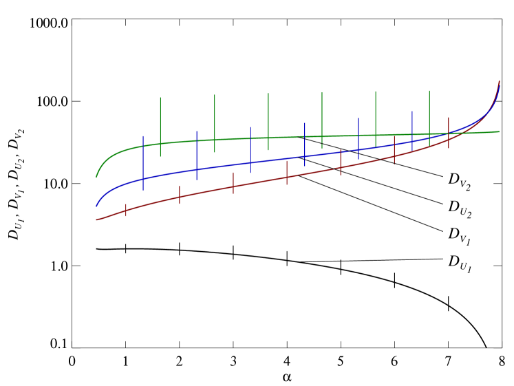
Figure 4: Linear theory for the two-layer Brusselator model, for $q=\sqrt{2-\sqrt{3}}=0.5176$, $\beta=1$, $A=3$, $B=9$, $r_{1}=0$ and $r_{q}=0$. We plot ${D_{U_{1}}}$ (black), ${D_{V_{1}}}$ (red), ${D_{U_{2}}}$ (blue) and ${D_{V_{2}}}$ (green) for $0.45\leq\alpha\leq 7.95$. The vertical lines indicate how the diffusion coefficients vary as $q$ ranges from $q=0.25$ to $q=0.66$: these coefficients generally decrease as $q$ increases. The vertical lines are at integer values of $\alpha$ for ${D_{U_{1}}}$ and ${D_{V_{1}}}$, and are shifted by $\frac{1}{3}$ for ${D_{U_{2}}}$ and by $\frac{2}{3}$ for ${D_{V_{2}}}$. Sample numerical values of the diffusion constants are given in Table 2 and in full in [40].

We solve the four polynomial equations numerically, using Bertini [41]. For our current choice of parameters, there are 24 solutions, of which eight are real but only two (related by relabelling the two layers) are real and positive:

$${D_{U_{1}}}=1.6046,\quad{D_{V_{1}}}=4.6663,\quad{D_{U_{2}}}=9.8682,\quad{D_{V_{2}}}=25.448.$$ (15)

The number of real positive solutions varies with $\alpha$ and $\beta$: for example, with $\beta=1$ and $q=\sqrt{2-\sqrt{3}}$, there are none for $\alpha\leq 0.31$ or $\alpha\geq 8$, and two (related by relabelling) for $0.32\leq\alpha\leq 7.99$. We plot the four diffusion coefficients as functions of $\alpha$ for $\beta=1$ in Figure 4 in black for $q=\sqrt{2-\sqrt{3}}=0.5176$, with vertical lines indicating how the diffusion coefficients vary with $q$, keeping $A$, $B$, $r_{1}$ and $r_{q}$ fixed. Sample numerical values of the diffusion constants for different choices of $\alpha$ and $q$ are given in Table 2 (below) and in full in [40].

We observe from Figure 4 that the range from the smallest to the largest values of the diffusion constants appears to diverge as $\alpha$ approaches $8$. The same happens for other choices of $q$. In addition, the ordering of the diffusion constants changes around $\alpha=7$: for $\alpha<7$, we have ${D_{U_{1}}}<{D_{V_{1}}}$ and ${D_{U_{2}}}<{D_{V_{2}}}$, which seems experimentally reasonable, in that one chemical diffuses slower than the other in either substrate, while for $\alpha>7$, this is not true. For later calculations, we will choose $\alpha$ to vary between $1$ and $7$. The experimental relevance of the larger values of $\alpha$ should be treated with caution.

Figure 5: Dispersion relation: the largest eigenvalue $\sigma(k)$ plotted as a function of wavenumber $k$, for $q=\sqrt{2-\sqrt{3}}=0.5176$, $\beta=1$, and $\alpha=1,2,\dots,7$.

We conclude our discussion of the linear theory with a sample dispersion relation ($\sigma(k)$ plotted as a function of wavenumber $k$) in Figure 5, for $q=\sqrt{2-\sqrt{3}}$ and for a range of $\alpha$, at the codimension-two point $r_{1}=r_{q}=0$. The eigenvalue is maximal at $k=q$ and $k=1$, but the minimum for $q<k<1$ is about $-0.1$ for $\alpha=1$, and only about $-0.015$ for $\alpha=7$.

In this dispersion relation, we control the separation and heights of the growth-rate maxima by varying $q$, $r_{1}$ and $r_{1}$, and solving for the four diffusion coefficients. For smaller $q$, the peaks are well separated and reasonably sharp, while for larger $q$ the peaks are closer together, broader and the depth of the minimum is less. For this reason, we limit ourselves to $q\leq 0.66$. Since we want to keep an interval of negative growth-rate between $k=q$ and $k=1$, we (mostly) limit ourselves to $r_{1}\leq 0.01$ and $r_{q}\leq 0.01$.

6 Weakly nonlinear theory

Once the uniform state $U_{1}=V_{1}=U_{2}=V_{2}=0$ becomes linearly unstable, solutions will grow exponentially until nonlinear effects become important. The first of these are the three-wave interactions. The weakly nonlinear theory is standard [28, 42, 43], though made more complicated here because of the codimension-two bifurcation and because there are four scalar fields in (9). We are concerned only with the leading order effect of three-wave interactions, and so we need to compute only up to second order in the weakly nonlinear theory.

We write

$${\bm{u}}=\begin{pmatrix}U_{1}\\ V_{1}\\ U_{2}\\ V_{2}\end{pmatrix},$$ (16)

and write the PDE (9) as

$$\frac{d{\bm{u}}}{dt}={\mathcal{L}}{\bm{u}}+\mbox{{{NLT}}$({\bm{u}})$},$$ (17)

where ${\mathcal{L}}$ is a linear operator representing the linear terms, and all the nonlinear terms in (9) are in NLT$({\bm{u}})$. To explore the properties of solutions close to ${\bm{u}}=0$, we introduce a small parameter $\epsilon\ll 1$, and we expand ${\bm{u}}$ in powers of $\epsilon$:

$${\bm{u}}=\epsilon{\bm{u}}_{1}+\epsilon^{2}{\bm{u}}_{2}+\cdots$$ (18)

Recall that in Section 5, we computed values of ${D_{U_{1}}}$, ${D_{V_{1}}}$, ${D_{U_{2}}}$ and ${D_{V_{2}}}$ such that the linear operator ${\mathcal{L}}$ had zero eigenvalues ($r_{1}=r_{q}=0$) at two wavenumbers, $k=1$ and $k=q$, at given values of $A$, $B$, $\alpha$ and $\beta$. We now suppose that the linear operator is perturbed by an order $\epsilon$ amount so that the growth rates $r_{1}$ at $k=1$ and $r_{q}$ at $k=q$ are order $\epsilon$. In practice we perturb ${D_{U_{1}}}$, ${D_{V_{1}}}$, ${D_{U_{2}}}$ and ${D_{V_{2}}}$ and do it in such a way that there are local maxima in the growth rate remain at $k=1$ and $k=q$. We can scale $r_{1}\rightarrow\epsilon r_{1}$ and $r_{q}\rightarrow\epsilon r_{q}$ and write the linear operator ${\mathcal{L}}$ as

$${\mathcal{L}}={\mathcal{L}}_{0}+\epsilon{\mathcal{L}}_{1}+\cdots,$$ (19)

where ${\mathcal{L}}_{0}$ is a singular linear operator, and $\epsilon{\mathcal{L}}_{1}$ is the largest part of the perturbation of the linear operator from ${\mathcal{L}}_{0}$. Finally, we scale time so that $d/dt\rightarrow\epsilon d/dt$. With these choices of scaling, the time derivative, the linear terms, and the lowest-order nonlinear terms all appear at the same order. Substituting into (17), we have

$$\epsilon^{2}\frac{d{\bm{u}}_{1}}{dt}=\epsilon{\mathcal{L}}_{0}{\bm{u}}_{1}+\epsilon^{2}{\mathcal{L}}_{0}{\bm{u}}_{2}+\epsilon^{2}{\mathcal{L}}_{1}{\bm{u}}_{1}+\epsilon^{2}\mbox{{{NLT}}${}_{2}({\bm{u}}_{1})$}+{\mathcal{O}}(\epsilon^{3}),$$ (20)

where NLT₂ represents the quadratic nonlinear terms.

The operator ${\mathcal{L}}_{0}$ is singular: ${\mathcal{L}}_{0}e^{i{\bm{k}}\cdot{\bm{x}}}{\bm{v}}_{1}=0$ whenever $|{\bm{k}}|=1$, and ${\mathcal{L}}_{0}e^{i{\bm{q}}\cdot{\bm{x}}}{\bm{v}}_{q}=0$ whenever $|{\bm{q}}|=q$, where ${\bm{v}}_{1}$ and ${\bm{v}}_{q}$ are the eigenvectors of the zero eigenvalues of the Jacobian matrix (11), with $k$ replaced by $1$ and $q$ respectively. We normalise the eigenvectors so that ${\bm{v}}_{1}\cdot{\bm{v}}_{1}=1$ and ${\bm{v}}_{q}\cdot{\bm{v}}_{q}=1$. Following the example of Section 5 and (15), with $A=3$, $B=9$, $\alpha=1$ and $\beta=1$, we find

$${\bm{v}}_{1}=\begin{pmatrix}\phantom{-}0.8416\\ -0.5198\\ \phantom{-}0.1377\\ -0.0496\end{pmatrix}\qquad\text{and}\qquad{\bm{v}}_{q}=\begin{pmatrix}\phantom{-}0.5288\\ -0.4550\\ \phantom{-}0.6201\\ -0.3589\end{pmatrix}.$$ (21)

With these eigenvectors, the general solution to ${\mathcal{L}}_{0}{\bm{u}}_{1}=0$ is similar to the expression in (1):

$${\bm{u}}_{1}=\left(\sum_{{\bm{q}}_{j}}w_{j}(t)e^{i{\bm{q}}_{j}\cdot{\bm{x}}}\right){\bm{v}}_{q}+\left(\sum_{{\bm{k}}_{j}}z_{j}(t)e^{i{\bm{k}}_{j}\cdot{\bm{x}}}\right){\bm{v}}_{1},$$ (22)

where $\{{\bm{q}}_{j}\}$ and $\{{\bm{k}}_{j}\}$ are arbitrary sets of vectors on the two circles $|{\bm{q}}_{j}|=q$ and $|{\bm{k}}_{j}|=1$. Writing ${\bm{u}}_{1}$ in this way solves the ${\mathcal{O}}(\epsilon)$ part of (20).

The ${\mathcal{O}}(\epsilon^{2})$ part of (20) is

$$\frac{d{\bm{u}}_{1}}{dt}={\mathcal{L}}_{0}{\bm{u}}_{2}+{\mathcal{L}}_{1}{\bm{u}}_{1}+\mbox{{{NLT}}${}_{2}({\bm{u}}_{1})$}.$$ (23)

Recall that ${\mathcal{L}}_{0}$ is singular and so cannot simply be inverted to find ${\bm{u}}_{2}$ as a function of ${\bm{u}}_{1}$. Thus, before solving for ${\bm{u}}_{2}$, a solvability condition must be imposed. The standard method is to define an inner product between vector-valued functions ${\bm{f}}({\bm{x}})$ and ${\bm{g}}({\bm{x}})$ on the domain $\Omega$ of the problem:

$$\big{\langle}{\bm{f}},{\bm{g}}\big{\rangle}=\frac{1}{|\Omega|}\int_{\Omega}{\bar{\bm{f}}}({\bm{x}})\cdot{\bm{g}}({\bm{x}})\,d{\bm{x}},$$ (24)

where ${\bar{\bm{f}}}$ is the complex conjugate of ${\bm{f}}$ and $|\Omega|$ is the area of the domain. We define ${\mathcal{L}}^{\dagger}_{0}$, the adjoint of ${\mathcal{L}}_{0}$, by requiring that

$$\big{\langle}{\bm{f}},{\mathcal{L}}_{0}{\bm{g}}\big{\rangle}=\big{\langle}{\mathcal{L}}^{\dagger}_{0}{\bm{f}},{\bm{g}}\big{\rangle}$$ (25)

for all ${\bm{f}}$ and ${\bm{g}}$. We restrict to functions on $\Omega$ that satisfy periodic boundary conditions. In this case, the adjoint operator ${\mathcal{L}}^{\dagger}_{0}$ is just the transpose of ${\mathcal{L}}_{0}$. Having defined ${\mathcal{L}}^{\dagger}_{0}$, we solve ${\mathcal{L}}^{\dagger}_{0}e^{i{\bm{k}}\cdot{\bm{x}}}{\bm{v}}^{\dagger}_{1}=0$ and ${\mathcal{L}}^{\dagger}_{0}e^{i{\bm{q}}\cdot{\bm{x}}}{\bm{v}}^{\dagger}_{q}=0$ to find the normalised adjoint eigenvectors ${\bm{v}}^{\dagger}_{1}$ and ${\bm{v}}^{\dagger}_{q}$, with $|{\bm{k}}|=1$ and $|{\bm{q}}|=q$. For our example, these are

$${\bm{v}}^{\dagger}_{1}=\begin{pmatrix}0.8416\\ 0.5198\\ 0.1377\\ 0.0496\end{pmatrix}\qquad\text{and}\qquad{\bm{v}}^{\dagger}_{q}=\begin{pmatrix}0.5288\\ 0.4550\\ 0.6201\\ 0.3589\end{pmatrix}.$$ (26)

Then, for any ${\bm{u}}_{2}$,

$$\begin{split}\Big{\langle}e^{i{\bm{k}}_{1}\cdot{\bm{x}}}{\bm{v}}^{\dagger}_{1},{\mathcal{L}}_{0}{\bm{u}}_{2}\Big{\rangle}&=\Big{\langle}{\mathcal{L}}^{\dagger}_{0}e^{i{\bm{k}}_{1}\cdot{\bm{x}}}{\bm{v}}^{\dagger}_{1},{\bm{u}}_{2}\Big{\rangle}=0,\\ \Big{\langle}e^{i{\bm{q}}_{1}\cdot{\bm{x}}}{\bm{v}}^{\dagger}_{q},{\mathcal{L}}_{0}{\bm{u}}_{2}\Big{\rangle}&=\Big{\langle}{\mathcal{L}}^{\dagger}_{0}e^{i{\bm{q}}_{1}\cdot{\bm{x}}}{\bm{v}}^{\dagger}_{q},{\bm{u}}_{2}\Big{\rangle}=0,\end{split}$$ (27)

where ${\bm{k}}_{1}$ and ${\bm{q}}_{1}$ represent any vectors on the two critical circles. Thus, taking the inner products of $e^{i{\bm{k}}_{1}\cdot{\bm{x}}}{\bm{v}}^{\dagger}_{1}$ and $e^{i{\bm{q}}_{1}\cdot{\bm{x}}}{\bm{v}}^{\dagger}_{q}$ with (23) results in the solvability conditions

$$\begin{split}\Big{\langle}e^{i{\bm{k}}_{1}\cdot{\bm{x}}}{\bm{v}}^{\dagger}_{1},\frac{d{\bm{u}}_{1}}{dt}\Big{\rangle}&=\Big{\langle}e^{i{\bm{k}}_{1}\cdot{\bm{x}}}{\bm{v}}^{\dagger}_{1},{\mathcal{L}}_{1}{\bm{u}}_{1}+\mbox{{{NLT}}${}_{2}({\bm{u}}_{1})$}\Big{\rangle},\\ \Big{\langle}e^{i{\bm{q}}_{1}\cdot{\bm{x}}}{\bm{v}}^{\dagger}_{q},\frac{d{\bm{u}}_{1}}{dt}\Big{\rangle}&=\Big{\langle}e^{i{\bm{q}}_{1}\cdot{\bm{x}}}{\bm{v}}^{\dagger}_{q},{\mathcal{L}}_{1}{\bm{u}}_{1}+\mbox{{{NLT}}${}_{2}({\bm{u}}_{1})$}\Big{\rangle}.\end{split}$$ (28)

Taking ${\bm{u}}_{1}$ to be made up of waves with wavevectors from all the combinations of wavevectors in Figure 2 results in amplitude equations (including the values of the coefficients) up to quadratic order, as written in (4). We will take two specific examples, focusing only on the quadratic coefficients, and compute $Q_{zh}$, $Q_{zz}$ and $Q_{zw}$. For these, we need NLT${}_{2}({\bm{u}}_{1})$, which is (for $A=3$ and $B=9$):

$$\mbox{{{NLT}}${}_{2}({\bm{u}}_{1})$}=\begin{pmatrix}\phantom{-}3U_{1}^{2}+6U_{1}V_{1}\\ -3U_{1}^{2}-6U_{1}V_{1}\\ \phantom{-}3U_{2}^{2}+6U_{2}V_{2}\\ -3U_{2}^{2}-6U_{2}V_{2}\end{pmatrix},$$ (29)

where $(U_{1},V_{1},U_{2},V_{2})$ are the four entries in ${\bm{u}}_{1}$.

To calculate the various quadratic coefficients described in Section 2, we take the combinations of wavevectors appropriate for each coefficient. For $Q_{zh}$, we write

$${\bm{u}}_{1}=\left(z_{1}(t)e^{i{\bm{k}}_{1}\cdot{\bm{x}}}+z_{2}(t)e^{i{\bm{k}}_{2}\cdot{\bm{x}}}+z_{3}(t)e^{i{\bm{k}}_{3}\cdot{\bm{x}}}\right){\bm{v}}_{1}+\text{c.c.},$$ (30)

where ${\bm{k}}_{1}={\bm{k}}_{2}+{\bm{k}}_{3}$ as in the top left panel of Figure 2, ${\bm{v}}_{1}$ is the eigenvector as in (21) and c.c. stands for the complex conjugate. In this case, we have

$$\begin{split}U_{1}^{2}&=\left(z_{1}e^{i{\bm{k}}_{1}\cdot{\bm{x}}}+z_{2}e^{i{\bm{k}}_{2}\cdot{\bm{x}}}+z_{3}e^{i{\bm{k}}_{3}\cdot{\bm{x}}}+\text{c.c.}\right)^{2}\times\left({\bm{v}}_{1}^{(1)}\right)^{2},\\ &=\left(\cdots+2z_{2}z_{3}e^{i{\bm{k}}_{1}\cdot{\bm{x}}}+\cdots\right)\times\left({\bm{v}}_{1}^{(1)}\right)^{2},\\ U_{1}V_{1}&=\left(z_{1}e^{i{\bm{k}}_{1}\cdot{\bm{x}}}+z_{2}e^{i{\bm{k}}_{2}\cdot{\bm{x}}}+z_{3}e^{i{\bm{k}}_{3}\cdot{\bm{x}}}+\text{c.c.}\right)^{2}\times\left({\bm{v}}_{1}^{(1)}{\bm{v}}_{1}^{(2)}\right),\\ &=\left(\cdots+2z_{2}z_{3}e^{i{\bm{k}}_{1}\cdot{\bm{x}}}+\cdots\right)\times\left({\bm{v}}_{1}^{(1)}{\bm{v}}_{1}^{(2)}\right),\end{split}$$ (31)

where we have highlighted the $e^{i{\bm{k}}_{1}\cdot{\bm{x}}}$ term, and ${\bm{v}}_{1}^{(1)}$ and ${\bm{v}}_{1}^{(2)}$ are the first and second entries in the vector ${\bm{v}}_{1}$ in (21). There are similar expressions for $U_{2}^{2}$ and $U_{2}V_{2}$, involving ${\bm{v}}_{1}^{(3)}$ and ${\bm{v}}_{1}^{(4)}$. The inner product with $e^{i{\bm{k}}_{1}\cdot{\bm{x}}}{\bm{v}}^{\dagger}_{1}$ in the first line of the solvability condition in (28) picks out the $e^{i{\bm{k}}_{1}\cdot{\bm{x}}}$ component of NLT${}_{2}({\bm{u}}_{1})$, so we are left with

$$\left({\bm{v}}^{\dagger}_{1}\cdot{\bm{v}}_{1}\right){\dot{z}_{1}}=\mbox{linear term}+{\bm{v}}^{\dagger}_{1}\cdot\begin{pmatrix}\phantom{-}3\times 2\left({\bm{v}}_{1}^{(1)}\right)^{2}+6\times 2{\bm{v}}_{1}^{(1)}{\bm{v}}_{1}^{(2)}\\ -3\times 2\left({\bm{v}}_{1}^{(1)}\right)^{2}-6\times 2{\bm{v}}_{1}^{(1)}{\bm{v}}_{1}^{(2)}\\ \phantom{-}3\times 2\left({\bm{v}}_{1}^{(3)}\right)^{2}+6\times 2{\bm{v}}_{1}^{(3)}{\bm{v}}_{1}^{(4)}\\ -3\times 2\left({\bm{v}}_{1}^{(3)}\right)^{2}-6\times 2{\bm{v}}_{1}^{(3)}{\bm{v}}_{1}^{(4)}\end{pmatrix}z_{2}z_{3}.$$ (32)

We have used the fact that ${\bm{v}}^{\dagger}_{1}$ is real. Dividing by ${\bm{v}}^{\dagger}_{1}\cdot{\bm{v}}_{1}$ and matching to (4) results in an expression for $Q_{zh}$. For the example set of parameters, $Q_{zh}=-0.7018$. With $r_{1}$ defined to be the growth rate (on the slow time scale) of the wavenumber $|{\bm{k}}|=1$ modes, the linear term above is $r_{1}\left({\bm{v}}^{\dagger}_{1}\cdot{\bm{v}}_{1}\right)z_{1}$.

Similar calculations but for different choices of wavevectors yield $Q_{wh}$, $Q_{zw}$ and $Q_{zz}$, and $Q_{wz}$ and $Q_{ww}$. We illustrate with the calculation for $Q_{zz}$ and $Q_{zw}$, and write

$${\bm{u}}_{1}=\left(z_{6}(t)e^{i{\bm{k}}_{6}\cdot{\bm{x}}}+z_{7}(t)e^{i{\bm{k}}_{7}\cdot{\bm{x}}}\right){\bm{v}}_{1}+\left(w_{1}(t)e^{i{\bm{q}}_{1}\cdot{\bm{x}}}\right){\bm{v}}_{q}+\text{c.c.},$$ (33)

where ${\bm{q}}_{1}={\bm{k}}_{6}+{\bm{k}}_{7}$ as in the middle row centre panel of Figure 2. In this case, we need the $e^{i{\bm{q}}_{1}\cdot{\bm{x}}}$ and $e^{i{\bm{k}}_{6}\cdot{\bm{x}}}$ components of $U_{1}^{2}$ and $U_{1}V_{1}$:

$$\begin{split}U_{1}^{2}&=\left(2z_{6}z_{7}e^{i{\bm{q}}_{1}\cdot{\bm{x}}}+\cdots\right)\times\left({\bm{v}}_{1}^{(1)}\right)^{2}+{}\\ &\qquad\left(2w_{1}{\bar{z}}_{7}e^{i{\bm{k}}_{6}\cdot{\bm{x}}}+\cdots\right)\times\left({\bm{v}}_{1}^{(1)}{\bm{v}}_{q}^{(1)}\right),\\ U_{1}V_{1}&=\left(2z_{6}z_{7}e^{i{\bm{q}}_{1}\cdot{\bm{x}}}+\cdots\right)\times\left({\bm{v}}_{1}^{(1)}{\bm{v}}_{1}^{(2)}\right)+{}\\ &\qquad\left(w_{1}{\bar{z}}_{7}e^{i{\bm{k}}_{6}\cdot{\bm{x}}}+\cdots\right)\times\left({\bm{v}}_{1}^{(1)}{\bm{v}}_{q}^{(2)}+{\bm{v}}_{1}^{(2)}{\bm{v}}_{q}^{(1)}\right),\end{split}$$ (34)

again with similar expressions for $U_{2}^{2}$ and $U_{2}V_{2}$. The inner product with $e^{i{\bm{k}}_{6}\cdot{\bm{x}}}{\bm{v}}^{\dagger}_{1}$ in the first line of the solvability condition in (28) picks out the $Q_{zw}{\bar{z}}_{7}w_{1}$ term, while the inner product with $e^{i{\bm{q}}_{1}\cdot{\bm{x}}}{\bm{v}}^{\dagger}_{q}$ in the second line of the solvability condition picks out the $Q_{zz}z_{6}z_{7}$ term. These result in equations for the two quadratic coefficients:

$$\begin{split}\left({\bm{v}}^{\dagger}_{1}\cdot{\bm{v}}_{1}\right)Q_{zw}&={\bm{v}}^{\dagger}_{1}\cdot\begin{pmatrix}\phantom{-}3\times 2{\bm{v}}_{1}^{(1)}{\bm{v}}_{q}^{(1)}+6\times\left({\bm{v}}_{1}^{(1)}{\bm{v}}_{q}^{(2)}+{\bm{v}}_{1}^{(2)}{\bm{v}}_{q}^{(1)}\right)\\ -3\times 2{\bm{v}}_{1}^{(1)}{\bm{v}}_{q}^{(1)}-6\times\left({\bm{v}}_{1}^{(1)}{\bm{v}}_{q}^{(2)}+{\bm{v}}_{1}^{(2)}{\bm{v}}_{q}^{(1)}\right)\\ \phantom{-}3\times 2{\bm{v}}_{1}^{(3)}{\bm{v}}_{q}^{(3)}+6\times\left({\bm{v}}_{1}^{(3)}{\bm{v}}_{q}^{(4)}+{\bm{v}}_{1}^{(4)}{\bm{v}}_{q}^{(3)}\right)\\ -3\times 2{\bm{v}}_{1}^{(3)}{\bm{v}}_{q}^{(3)}-6\times\left({\bm{v}}_{1}^{(3)}{\bm{v}}_{q}^{(4)}+{\bm{v}}_{1}^{(4)}{\bm{v}}_{q}^{(3)}\right)\end{pmatrix},\\ \left({\bm{v}}^{\dagger}_{q}\cdot{\bm{v}}_{q}\right)Q_{zz}&={\bm{v}}^{\dagger}_{q}\cdot\begin{pmatrix}\phantom{-}3\times 2\left({\bm{v}}_{1}^{(1)}\right)^{2}+6\times 2{\bm{v}}_{1}^{(1)}{\bm{v}}_{1}^{(2)}\\ -3\times 2\left({\bm{v}}_{1}^{(1)}\right)^{2}-6\times 2{\bm{v}}_{1}^{(1)}{\bm{v}}_{1}^{(2)}\\ \phantom{-}3\times 2\left({\bm{v}}_{1}^{(3)}\right)^{2}+6\times 2{\bm{v}}_{1}^{(3)}{\bm{v}}_{1}^{(4)}\\ -3\times 2\left({\bm{v}}_{1}^{(3)}\right)^{2}-6\times 2{\bm{v}}_{1}^{(3)}{\bm{v}}_{1}^{(4)}\end{pmatrix}.\end{split}$$ (35)

For the example set of parameters, $Q_{zw}=-0.8974$ and $Q_{zz}=-0.1997$. Similar calculations yield $Q_{wh}=-0.5610$, and $Q_{wz}=-0.2623$ and $Q_{ww}=-0.9263$ (only available since $q>\frac{1}{2}$).

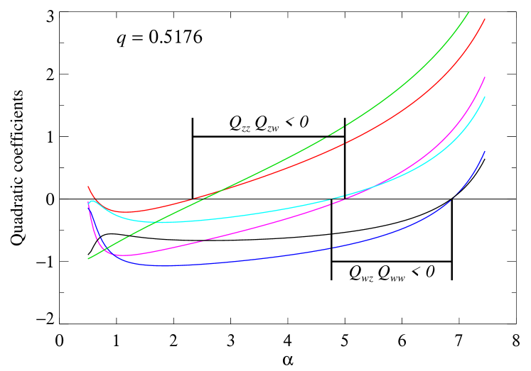
Figure 6: Weakly nonlinear theory for the two-layer Brusselator model (9), up to quadratic order. We take $\beta=1$ in (9) and $q=0.5176$ in (1). The six quadratic coefficients are $Q_{zh}$ (green), $Q_{wh}$ (black), $Q_{zz}$ (red), $Q_{zw}$ (magenta), $Q_{wz}$ (cyan), $Q_{ww}$ (blue). In this case, the coefficients $Q_{zw}$ and $Q_{zz}$ have opposite sign for $2.33<\alpha<5.00$, and $Q_{wz}$ and $Q_{ww}$ have opposite sign for $4.76<\alpha<6.87$. The values of diffusion coefficients are as in Figure 4. The data for this figure is available in full at [40], with selected values in Table 2.

$q$	$\alpha$	${D_{U_{1}}}$	${D_{V_{1}}}$	${D_{U_{2}}}$	${D_{V_{2}}}$	$Q_{zh}$	$Q_{wh}$	$Q_{zz}$	$Q_{zw}$	$Q_{wz}$	$Q_{ww}$
	$1$	$1.75$	$\phantom{0}5.2$	$16.4$	$44.0$	$-0.59$	$-0.52$	$-0.07$	$-0.85$	—	—
	$2$	$1.76$	$\phantom{0}8.1$	$21.2$	$53.9$	$\phantom{-}0.02$	$-0.57$	$\phantom{-}0.04$	$-0.79$	—	—
	$3$	$1.59$	$11.2$	$25.2$	$57.9$	$\phantom{-}0.57$	$-0.62$	$\phantom{-}0.31$	$-0.60$	—	—
$0.3780$	$4$	$1.34$	$15.0$	$29.5$	$60.4$	$\phantom{-}1.12$	$-0.64$	$\phantom{-}0.64$	$-0.36$	—	—
	$5$	$1.05$	$20.0$	$34.7$	$62.3$	$\phantom{-}1.71$	$-0.62$	$\phantom{-}1.05$	$-0.07$	—	—
	$6$	$0.73$	$28.0$	$42.3$	$64.1$	$\phantom{-}2.41$	$-0.55$	$\phantom{-}1.59$	$\phantom{-}0.33$	—	—
	$7$	$0.38$	$45.2$	$57.5$	$65.9$	$\phantom{-}3.36$	$-0.29$	$\phantom{-}2.41$	$\phantom{-}1.05$	—	—
	$1$	$1.60$	$\phantom{0}4.7$	$\phantom{0}9.9$	$25.4$	$-0.70$	$-0.56$	$-0.20$	$-0.90$	$-0.26$	$-0.93$
	$2$	$1.55$	$\phantom{0}6.8$	$13.7$	$32.0$	$-0.23$	$-0.65$	$-0.08$	$-0.78$	$-0.37$	$-1.07$
	$3$	$1.38$	$\phantom{0}9.1$	$16.8$	$34.8$	$\phantom{-}0.21$	$-0.66$	$\phantom{-}0.18$	$-0.56$	$-0.29$	$-1.01$
$0.5176$	$4$	$1.16$	$11.9$	$20.1$	$36.6$	$\phantom{-}0.66$	$-0.62$	$\phantom{-}0.50$	$-0.31$	$-0.15$	$-0.90$
	$5$	$0.90$	$15.6$	$24.1$	$37.9$	$\phantom{-}1.17$	$-0.53$	$\phantom{-}0.89$	$\phantom{-}0.00$	$\phantom{-}0.06$	$-0.74$
	$6$	$0.63$	$21.5$	$29.7$	$39.2$	$\phantom{-}1.81$	$-0.35$	$\phantom{-}1.42$	$\phantom{-}0.44$	$\phantom{-}0.38$	$-0.48$
	$7$	$0.33$	$34.0$	$40.8$	$40.5$	$\phantom{-}2.77$	$\phantom{-}0.10$	$\phantom{-}2.25$	$\phantom{-}1.24$	$\phantom{-}1.02$	$\phantom{-}0.11$
	$1$	$1.48$	$\phantom{0}4.2$	$\phantom{0}7.7$	$19.3$	$-0.77$	$-0.61$	$-0.33$	$-0.92$	$-0.41$	$-0.98$
	$2$	$1.40$	$\phantom{0}6.0$	$11.0$	$24.7$	$-0.38$	$-0.69$	$-0.20$	$-0.76$	$-0.46$	$-1.01$
	$3$	$1.24$	$\phantom{0}8.0$	$13.7$	$26.9$	$-0.00$	$-0.65$	$\phantom{-}0.05$	$-0.54$	$-0.34$	$-0.90$
$0.6180$	$4$	$1.04$	$10.3$	$16.5$	$28.4$	$\phantom{-}0.39$	$-0.57$	$\phantom{-}0.35$	$-0.28$	$-0.17$	$-0.76$
	$5$	$0.81$	$13.4$	$19.8$	$29.5$	$\phantom{-}0.85$	$-0.43$	$\phantom{-}0.72$	$\phantom{-}0.03$	$\phantom{-}0.07$	$-0.56$
	$6$	$0.56$	$18.3$	$24.6$	$30.5$	$\phantom{-}1.45$	$-0.18$	$\phantom{-}1.23$	$\phantom{-}0.49$	$\phantom{-}0.43$	$-0.24$
	$7$	$0.29$	$28.7$	$33.9$	$31.6$	$\phantom{-}2.40$	$\phantom{-}0.38$	$\phantom{-}2.07$	$\phantom{-}1.31$	$\phantom{-}1.14$	$\phantom{-}0.44$

Table 2: Sample values of the diffusion coefficients in (9) and the resulting quadratic coefficients in (4), with $A=3$, $B=9$, $\beta=1$, $r_{1}=0$ and $r_{q}=0$, for different choices of $q$ and $\alpha$. The data are illustrated in Figures 4 and 6. A fuller version of this table (for $0.25\leq q\leq 0.66$) is available in full in [40].

Examples of the six quadratic coefficients as functions of $\alpha$ are shown in Figure 6, for $q=\sqrt{2-\sqrt{3}}=0.5176$, and for $\beta=1$, with numerical values for this and other choices of $q$ given in Table 2 and in [40].

With this choice of parameters, the coefficients $Q_{zw}$ and $Q_{zz}$ have opposite sign for $2.33<\alpha<5.00$, and $Q_{wz}$ and $Q_{ww}$ have opposite sign for $4.76<\alpha<6.87$. The behaviour of the quadratic coefficients for other values of $q$ in the range $0.25\leq q\leq 0.66$ is similar: there is a range of $\alpha$ for which $Q_{zw}Q_{zz}<0$, and (provided $q>\frac{1}{2}$) there is a range of $\alpha$ for which $Q_{wz}Q_{ww}<0$, where the ordering is the same throughout. The two ranges overlap over a limited range of $\alpha$, centred on $\alpha\approx 4.8$ for all $q$.

$q$	$\theta_{z}$	$\theta_{w}$	Comment
$0.2500$	$165.6^{\circ}$	—
$0.3300$	$161.0^{\circ}$	—
$0.3780$	$158.2^{\circ}$	—	$q=1/\sqrt{7}$: superlattice patterns
$0.4400$	$154.6^{\circ}$	—
$0.5176$	$150.0^{\circ}$	$30.0^{\circ}$	$q=\sqrt{2-\sqrt{3}}$: twelve-fold quasipatterns
$0.5500$	$148.1^{\circ}$	$49.2^{\circ}$
$0.5774$	$146.4^{\circ}$	$60.0^{\circ}$	$q=1/\sqrt{3}$: hexagons
$0.6180$	$144.0^{\circ}$	$72.0^{\circ}$	$q=\frac{1}{2}(-1+\sqrt{5})$: ten-fold quasipatterns
$0.6600$	$141.5^{\circ}$	$81.5^{\circ}$

Table 3: Values of the length scale ratio $q$ used in our survey. The angles $\theta_{z}$ and $\theta_{w}$ are defined in Figure 2 and Eq. (3).

7 Numerical results

Based on the linear and weakly nonlinear calculations in the previous sections, we have carried out a series of numerical simulations of the PDEs in (9). Our main goal is to explore the effect of varying the ratio of length scales, $q$, in regimes where we can control the signs of the quadratic coefficients. Our choice is to fix the diffusive coupling coefficient $\beta=1$ and vary $\alpha$ with $1\leq\alpha\leq 7$ (in steps of 1). With different choices of $\alpha$, the two pairs of quadratic coefficients can have the same or opposite signs (see Figure 6), though the range where both pairs had opposite sign was very limited. We chose some special values of $q$, some less than and some greater than $\frac{1}{2}$: $q=1/\sqrt{7}=0.3780$, to encourage superlattice patterns [44]; $q=\sqrt{2-\sqrt{3}}=0.5176$, to encourage twelve-fold quasipatterns [38, 39]; $q=1/\sqrt{3}=0.5774$, to allow quadratic interactions between six modes on each circle; and $q=\frac{1}{2}(-1+\sqrt{5})=0.6180$, to encourage ten-fold quasipatterns [45]. We also chose more “generic” values of $q$: $0.25$, $0.33$, $0.44$, $0.55$ and $0.66$. The values of $q$ and the corresponding angles $\theta_{z}$ and $\theta_{w}$ are listed in Table 3. All chemical properties are frozen with the choice of $A=3$ and $B=9$ as in [10].

The values of the diffusion coefficients at the codimension-two point $r_{1}=r_{q}=0$ are given in Figure 4 and in [40]. For each selected case of $q$ and $\alpha$, we vary the diffusion coefficients to explore small positive and negative values of the two growth rates $r_{1}$ and $r_{q}$. Specifically, setting $(r_{1},r_{q})=(r\cos\theta,r\sin\theta)$, we choose $r=0.01$ (apart from data in Figure 11), with $\theta$ varying from $5^{\circ}$ to $355^{\circ}$ in steps of $10^{\circ}$. For smaller $q$ and $\alpha$, these choices lead to growth rates $\sigma(k)$ that are sharply peaked at $k=q$ and $k=1$, with a relatively deep negative minimum in between (see Figure 5). However, for larger $q$ and $\alpha$, the minimum between the two maxima is quite shallow, which means that, even with a small value of $r=0.01$, there can be wide bands of unstable wavenumbers.

We start all simulations from small-amplitude random initial conditions in $16\pi\times 16\pi$ ($8\times 8$ of the shorter wavelengths) domains, except in the case when $q=\sqrt{2-\sqrt{3}}$ where we also start simulations from a small-amplitude quasipattern initial condition. For parameter choices that do not result in a simple pattern, we explore the effect of a larger domain by re-running calculations in $60\pi\times 60\pi$ ($30\times 30$ wavelengths) domains. Both $8\times 8$ and $30\times 30$ domains are appropriate for twelve-fold quasipatterns [46]. Time simulations are for at least 10000 time units: this is 100 growth times (for $r=0.01$) and approximately three diffusion times for the larger domain when considering the smallest values of the diffusion coefficients.

We use $128\times 128$ Fourier modes (using FFTW [47], the fastest Fourier transform in the West) in each direction for the $8\times 8$ domains, and $512\times 512$ Fourier modes for the larger $30\times 30$ domains. We use the second-order exponential time differencing (ETD2) [48] scheme for timestepping, with a fixed timestep of 0.01. For this matrix exponential method, we split the linear part of the PDE (9) into diagonal and off-diagonal parts, and we treat the off-diagonal parts as nonlinear terms.

In all, we carried out over 4000 simulations, and the results we present below are an overview of the range of patterns we find. For $\alpha\leq 3$, we find a wide range of different patterns, but for $\alpha\geq 4$ we find simple patterns (hexagons) almost exclusively. Therefore, we focus on the cases with $\alpha=1$, 2 and 3. When $\alpha=1$, all quadratic coefficients are negative for all $q$ (see Figure 6, Table 2 and [40]). Therefore, from Table 1, we expect to find only steady patterns. For $\alpha=2$, $Q_{zw}$ and $Q_{zz}$ are of opposite sign for $q\in\{0.2500,0.3300,0.3780\}$ and are of the same sign for $q\in\{0.4400,0.5176,0.5774,0.6180,0.6600\}$, although $Q_{zz}$ is very close to zero for $q=0.4400$. For $\alpha=3$, $Q_{zw}$ and $Q_{zz}$ are of opposite sign for all $q$ apart from $q=0.6600$. For $1\leq\alpha\leq 3$, $Q_{wz}$ and $Q_{ww}$ are both negative. We connect some of the observed steady patterns in this section to the three cases of nonlinear wave-vector interactions described in Figure 3 and relate these to our expectations in Table 1.

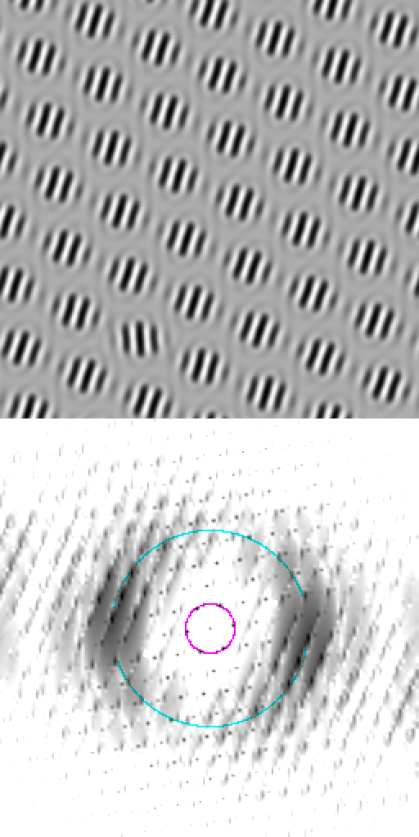
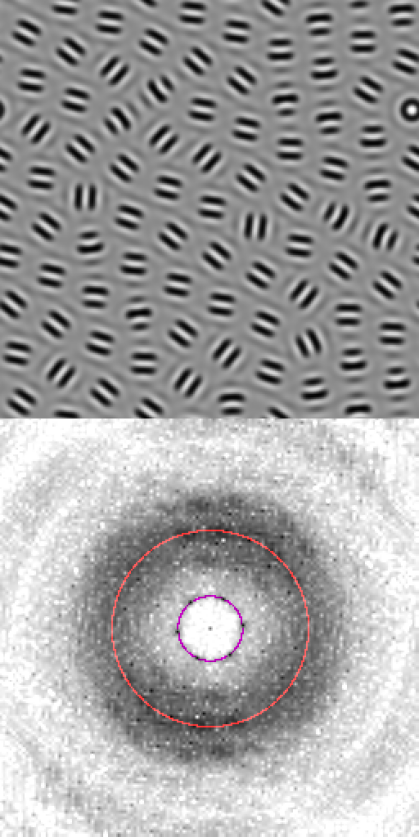
(a) $q=0.2500$ (b) $q=0.3300$ (c) $q=0.3780$ (d) $q=0.4400$

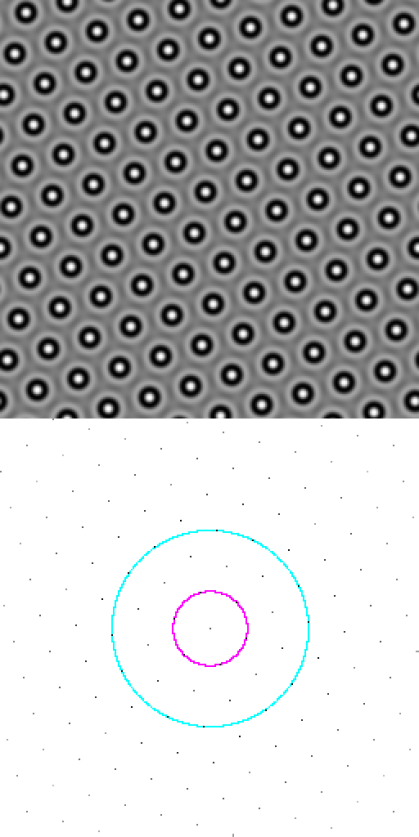
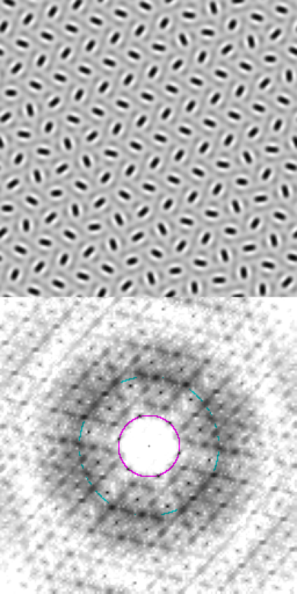
Figure 7: Examples of patterns, all in $30\times 30$ domains for $\alpha=1$ and $r=0.01$, $\theta=45^{\circ}$, with $q$ running from $0.25$ to $0.66$. Each image has a grey scale representing $U_{1}({\bm{x}})$ (the scaling is different in each case) and a power spectrum with circles $k=1$ and $k=q$ indicated.

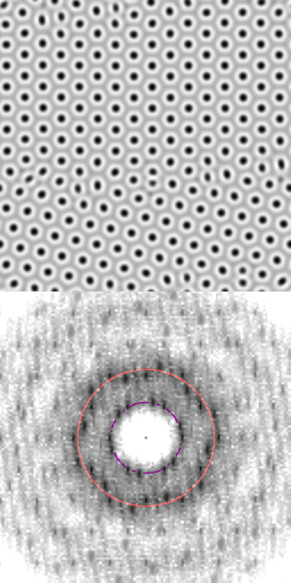
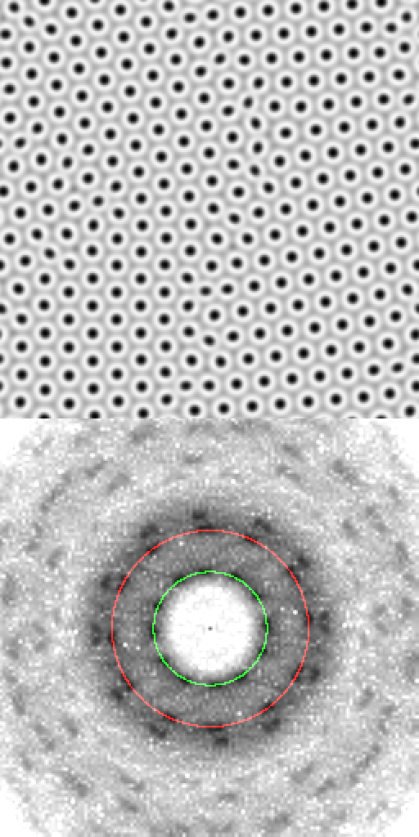
(e) $q=0.5176$ (f) $q=0.5774$ (g) $q=0.6180$ (h) $q=0.6600$

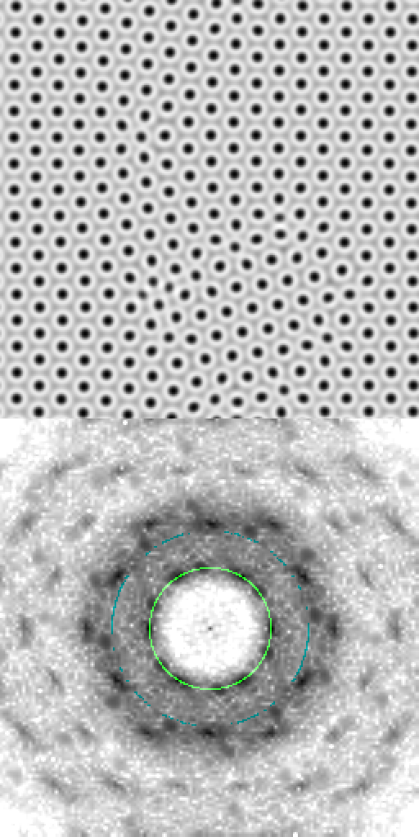
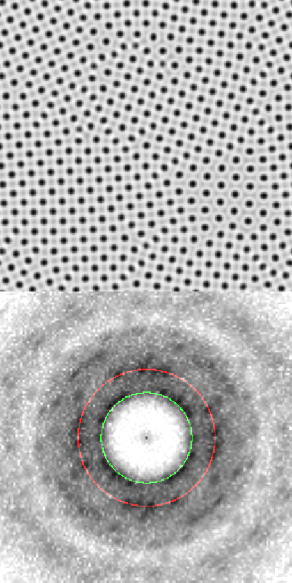
Figure 7: Continued from previous page.

7.1 Steady patterns with varying $q$: $\alpha=1$

First, we explore steady patterns with $\alpha=1$ at fixed $r=0.01$ and $\theta=45^{\circ}$, so $r_{1}=r_{q}=0.00707$, but for varying $q$ (see Figure 7). For $q<\frac{1}{2}$, we see strong hexagonal motifs on a scale set by the smaller wavenumber $q$, inset with stripes on a scale of wavenumber 1, resembling patterns found by [10]. For $q=0.3780$ the pattern is exactly hexagonal, with six equally spaced modes on the inner circle and twelve unequally spaced on the outer, as in Figure 3(a) – this is the simplest example of a superlattice pattern. As $q$ increases beyond 0.5176, the patterns continue as essentially hexagonal on the scale of the smaller wavenumber, but defects and grain boundaries become more common for larger $q$.

(a) $\alpha=1$, $q=0.5176$ (b) $\alpha=2$, $q=0.2500$

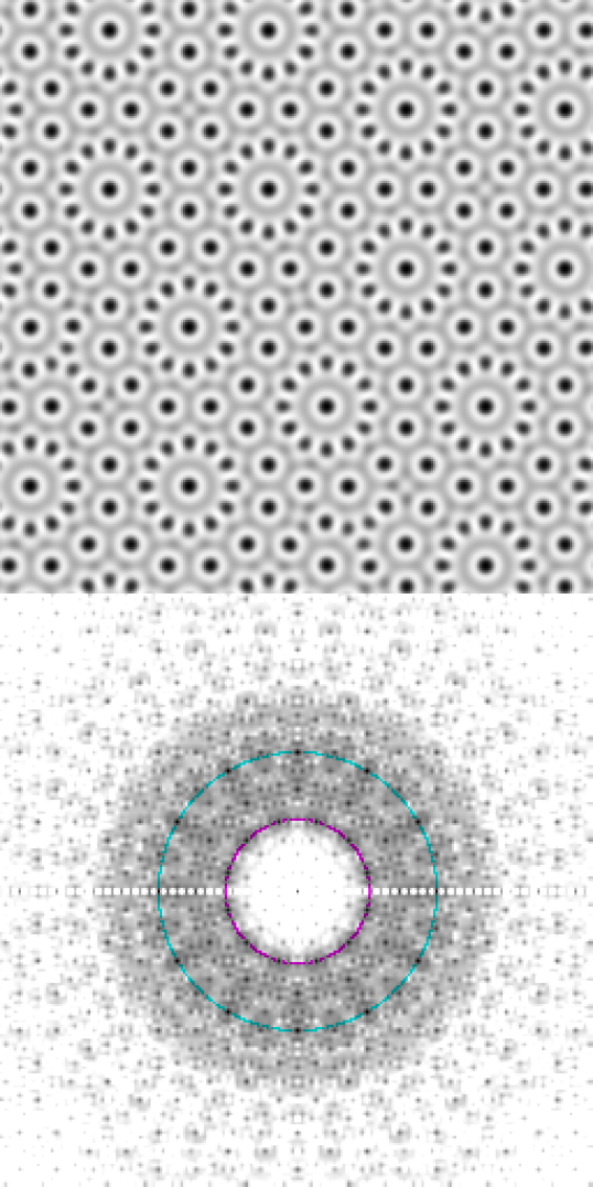
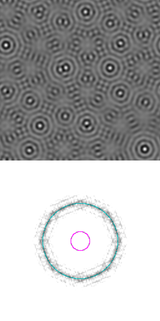
Figure 8: Examples of quasipatterns. (a) A twelve-fold quasipattern with $\alpha=1$, $q=0.5176$, $\theta=315^{\circ}$. (b) An eight-fold approximate quasipattern with $\alpha=2$, $q=0.2500$, $\theta=165^{\circ}$.

7.2 Quasipatterns

We take $q=\sqrt{2-\sqrt{3}}=0.5176$ and start with small amplitudes for twelve Fourier modes on the circle $k=1$ as initial condition to encourage twelve-fold quasipatterns, finding stable examples as in Figure 8(a). This is a periodic approximant to a true quasipattern, but the approximation is particularly accurate in the $30\times 30$ domain [46]. There are twelve peaks on the inner and outer circles, interleaved as in Figure 3(b). This kind of quasipattern has been seen in many similar kinds of calculations going back to [38, 39].

We also obtain an eight-fold quasipattern, in Figure 8(b). This is surprising since neither $\theta_{z}$ nor $\theta_{w}$ is a multiple of $45^{\circ}$ (Table 3). In addition, in our $30\times 30$ domain, the approximation to a true eight-fold quasipattern is not particularly accurate. Nonetheless, there are eight reasonably clear peaks on the inner circle, with sixteen diffuse peaks on the outer and an additional eight peaks just outside the outer circle, giving the impression of a regular octagon. It may be significant that $\theta_{z}=165.6^{\circ}$ (see Table 3), which is close to $15^{\circ}$ less than $180^{\circ}$, as the twenty-four peaks on and just off the outer circle are spaced roughly $15^{\circ}$ apart.

The third common two-dimensional quasipattern has ten-fold symmetry. We have not found examples of such a quasipattern, but there are hints of a ten-fold motif in calculations with $q=0.6180$ (see Figure 9b).

(a) $\alpha=2$, $q=0.5176$ (b) $\alpha=2$, $q=0.6180$

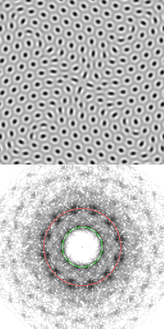
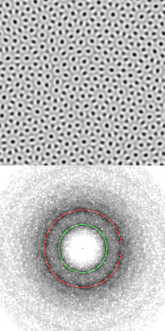
Figure 9: Examples of steady (or persistent) complex patterns. (a) Swirly distorted hexagonss with $\alpha=2$, $q=0.5176$, $\theta=45^{\circ}$. After a transient of about 20000 time units, these are replaced by hexagons. (b) Hints of ten-fold quasipattern motifs with $\alpha=2$, $q=0.6180$, $\theta=275^{\circ}$. This complex pattern persists for at least 50000 time units.

7.3 Steady complex patterns

We find many examples of hexagonal patterns with defects as in Figure 7(e–h). In Figure 9, we show two examples of steady complex patterns that are not just straightforward patches of hexagons (as in Figure 7e–h). In Figure 9(a), with $q=0.5176$, the pattern has a “swirly” appearance with regions of distorted hexagons in between patches of more regular hexagons. The patches are rotated with respect to each other, leading to twelve broad peaks in the outer circle of the power spectrum. In Figure 9(b), with $q=0.6180$, the complex structure of the pattern is more uniformly distributed, both in space and around the two circles in the power spectrum. There are several examples of a ten-fold motif, not surprising given that $q$ is the inverse of the golden ratio.

Both examples are not steady but continue to evolve on timescales longer than 10000 time units. The example in Figure 9(a) eventually anneals to hexagons. The example in Figure 9(b) persists for at least 50000 time units, and is the closest we have found to an example of a steady complex pattern with the infinite set of wavevectors implied by Figure 3(c).

(a) $\alpha=2$, $q=0.4400$

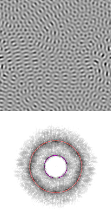
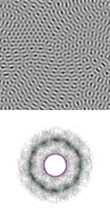
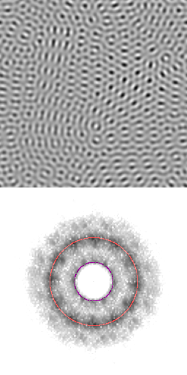
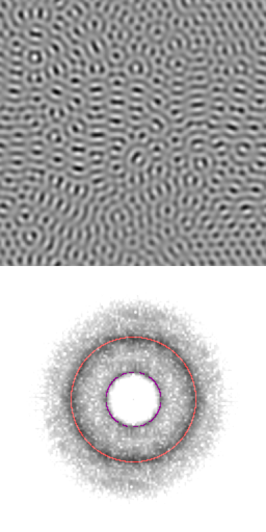
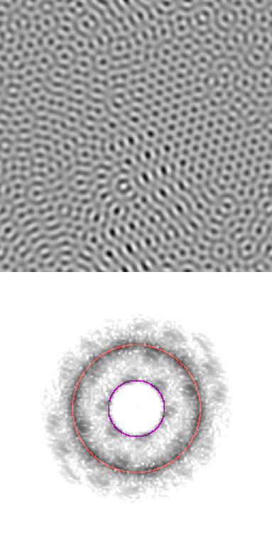
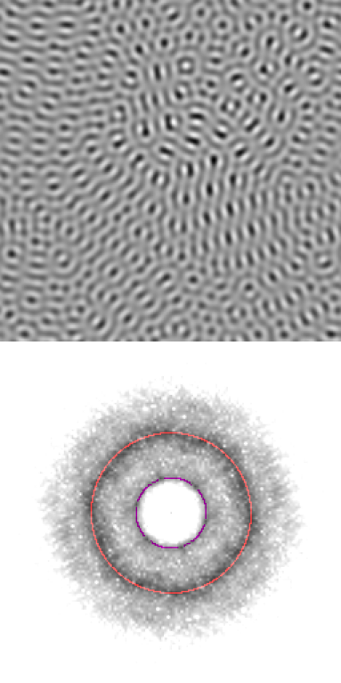
Figure 10: Frames from two examples of spatiotemporal chaos. (a) $\alpha=2$, $q=0.4400$, $\theta=5^{\circ}$. (b) $\alpha=3$, $q=0.6180$, $\theta=45^{\circ}$. The time interval between frames is 2000 time units. Videos are available in [40].

(b) $\alpha=3$, $q=0.6180$

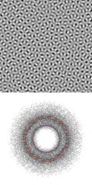
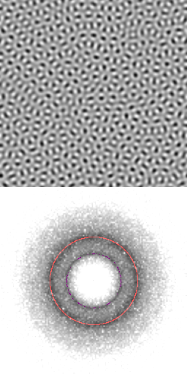
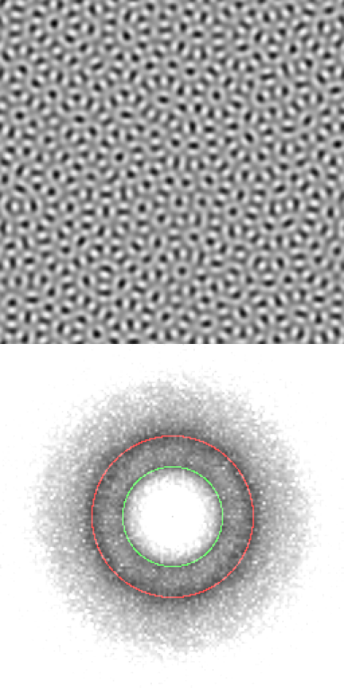
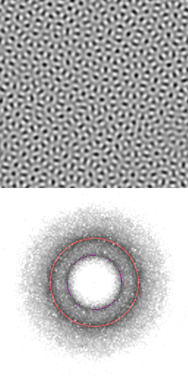
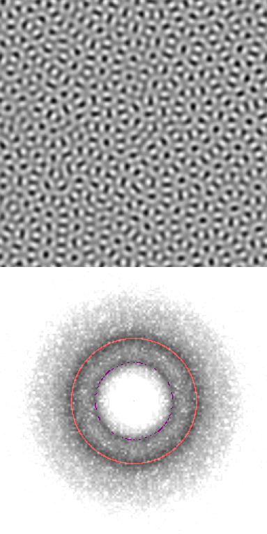
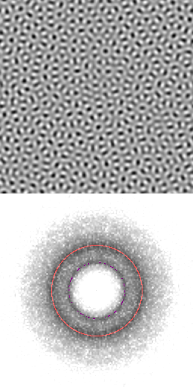
Figure 10: Continued from previous page.

$\alpha=3$, $q=0.3780$

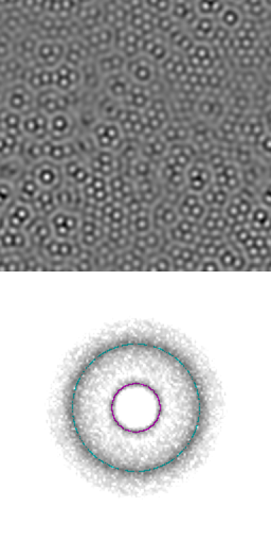
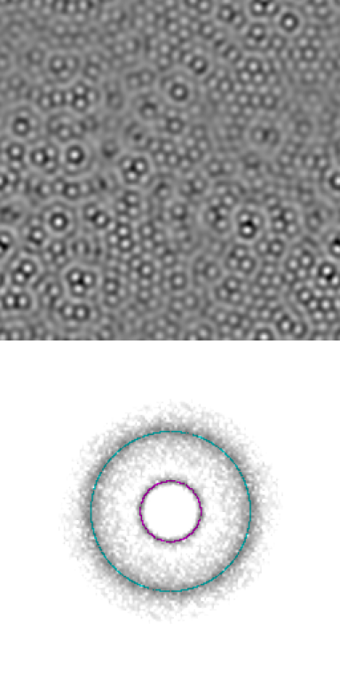
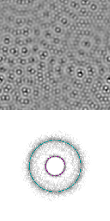
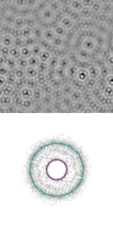
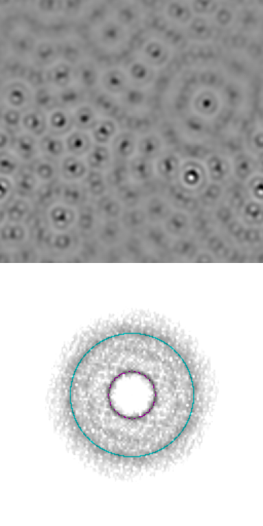
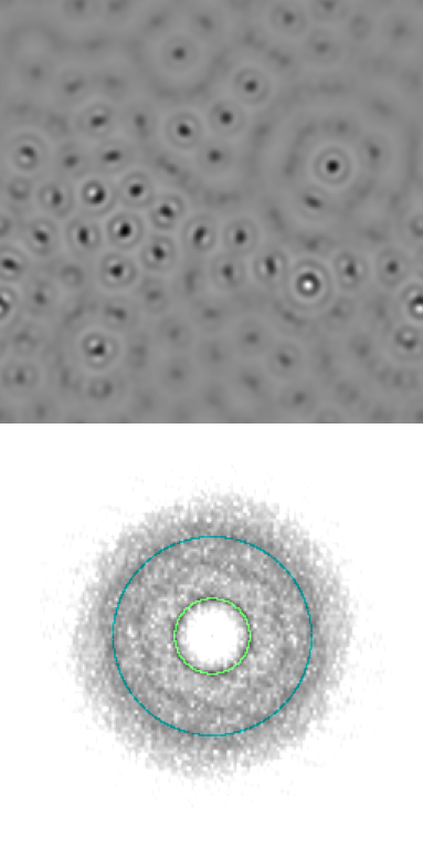
Figure 11: Frames from an examples of spatiotemporal chaos: $\alpha=3$, $q=0.3780$, $r=0.03$, $\theta=145^{\circ}$. This example evolves much more quickly than those of Figure 10: the time interval between frames is 20 time units. A video is available in [40].

7.4 Spatiotemporal chaos

Finally, we show three examples of spatiotemporal chaos in Figure 10(a) and (b), with $q=0.4400$ and $q=0.6180$ respectively, and in Figure 11, with $q=0.3780$ but with larger linear parameters than the others calculations ($r=0.03$). The spatiotemporal chaos examples in Figure 10 evolve quite slowly: a frame spacing of 2000 time units is needed to show appreciable differences between the frames. The frame spacing in Figure 11 is 100 times less. Videos of all three examples are available in [40].

In the $q<\frac{1}{2}$ example in Figure 10(a), there are evolving patches of elongated hexagons, and in some frames, the power spectrum has twelve peaks on the outer circle. In contrast, the $q>\frac{1}{2}$ example in Figure 10(b) has a much more axisymmetric power spectrum and the complexity of the pattern is more uniformly spread across the domain. In the third example in Figure 11, the system alternates between episodes dominated by small hexagons and episodes dominated by larger structures.

8 Summary and Discussion

One main finding is that we only find persistent time dependence (as opposed to slow healing of defects and coarsening of grain boundaries) when $Q_{zw}$ and $Q_{zz}$ had opposite sign, as in Figures 10 and 11. This is consistent with our a priori expectations outlined in Table 1. With appropriate initial conditions, we find twelve-fold quasipatterns only in the case with $q=\sqrt{2-\sqrt{3}}$, although we find eight-fold and hints of ten-fold quasipatterns in other cases. We did find examples of steady (or persistent) complex patterns, as in Figure 9. It was noticeable that having two interacting wavelengths encourages patterns with defects.

With quadratic coefficients $Q_{zw}$ and $Q_{zz}$ of opposite sign, the preliminary $8\times 8$ calculations often yield time-dependent patterns, with relatively simple oscillatory, chaotic or heteroclinic cycle dynamics. When we extend these into $30\times 30$ domains, the simple time dependence is often replaced by spatiotemporal chaos, supporting the infinite set of wavevectors picture implied by Figure 3(c). We suspect that the reason for this is that in $8\times 8$ domains, there are relatively few modes available close enough to each circle to participate in the dynamics. In contrast, with $30\times 30$ domains, the density of modes in Fourier space is higher, and so modes are more likely to be able to participate in multiple three-wave interactions, as in Figure 2. Considering a single set of modes coupled by a three-wave interaction, the modes may be oscillatory. When two (or more) sets of modes, also coupled within themselves by three-wave interaction, have modes in common, the common modes will be torn in different directions by their partners in the different sets, resulting in spatiotemporal chaos.

All interesting cases of time dependence have $Q_{zw}$ and $Q_{zz}$ of opposite sign, and time dependence can happen for all values of $q$. Having $Q_{wz}$ and $Q_{ww}$ of opposite sign (relevant only for $q>\frac{1}{2}$) did not lead to persistent time dependence. Having $q>\frac{1}{2}$ did appear to help when seeking steady complex patterns (Figure 9b): we find no examples of such patterns with $q<\frac{1}{2}$. This is in contrast to the hypotheses of [27], who argued that having $q>\frac{1}{2}$ and having $Q_{wz}$ and $Q_{ww}$ of opposite sign should encourage complex patterns. In fact, we find that $q<\frac{1}{2}$ is more interesting than anticipated from the results of [27], especially when $Q_{zw}$ and $Q_{zz}$ have opposite sign: there are many more states possible, including spatiotemporal chaos, going well beyond the steady superlattice example associated with $q=1/\sqrt{7}=0.3780$, in Figure 7(c). We also had not anticipated finding quasipatterns in the case $q<\frac{1}{2}$ (as in Figure 8b), but recent work [29] suggests this warrants more exploration.

In summary, our main numerical findings described above are broadly in line with the a priori expectations in Table 1. In particular, time dependence, and with it complex spatial structure, requires $Q_{zw}$ and $Q_{zz}$ to have opposite sign. The other pair of quadratic coefficients ($Q_{wz}$ and $Q_{ww}$) can also have opposite sign for $\alpha=5$ and 6, but for these values, we mainly find domains of hexagons. At this point, it is not clear why this happens, nor whether other systems would behave differently. We should emphasise that the time-dependence we have found is not associated with a primary Hopf bifurcation to spiral waves, common in many Turing systems.

It would be interesting to explore these complex patterns in more detail, in the context of coupled reaction–diffusion systems, in the context of amplitude equations, especially in the case $q<\frac{1}{2}$, as initiated in [49], and in the context of simpler model PDEs, such as the ones proposed by [38, 39, 27, 46] as models for Faraday waves. A related PDE is known to produce three-dimensional icosahedral quasipatterns [50] and localised quasipatterns [51], and such structures may also be possible in Turing systems. We plan to undertake further investigations in the future.

Of course, one has to ask whether these kinds of patterns can be found in experiments, and indeed if the mechanisms for forming them are as outlined in this paper. As explained in [13], manipulating the strength of the coupling, and indeed the diffusion constants, as we have done here, is difficult. Nonetheless, the spatially complex experimental patterns reported in [13] (see Figure 1) resemble, at least qualitatively, the images in Figures 10 and 11.

References

- [1] A. M. Turing, The chemical basis of morphogenesis, Phil. Trans. R. Soc. Lond. B 237 (1952) 37–72.
- [2] J. H. Dawes, After 1952: The later development of Alan Turing’s ideas on the mathematics of pattern formation, Hist. Math. 43 (2016) 49–64.
- [3] V. Castets, E. Dulos, J. Boissonade, P. DeKepper, Experimental evidence of a sustained standing Turing-type nonequilibrium chemical pattern, Phys. Rev. Lett. 64 (1990) 2953–2956.
- [4] A. Nakamasu, G. Takahashi, A. Kanbe, S. Kondo, Interactions between zebrafish pigment cells responsible for the generation of Turing patterns, Proc. Natl. Acad. Sci. 106 (2009) 8429–8434.
- [5] J. H. Cartwright, Labyrinthine Turing pattern formation in the cerebral cortex, J. Theor. Biol. 217 (2002) 97–103.
- [6] C. A. Klausmeier, Regular and irregular patterns in semiarid vegetation, Science 284 (1999) 1826–1888.
- [7] S. A. Levin, L. A. Segel, Hypothesis for origin of planktonic patchiness, Nature 259 (1976) 659.
- [8] S. Kondo, T. Miura, Reaction-diffusion model as a framework for understanding biological pattern formation, Science 329 (2010) 1616–1620.
- [9] P. K. Maini, T. E. Woolley, R. E. Baker, E. A. Gaffney, S. S. Lee, Turing’s model for biological pattern formation and the robustness problem, Interface Focus 2 (2012) 487–496.
- [10] L. Yang, M. Dolnik, A. M. Zhabotinsky, I. R. Epstein, Spatial resonances and superposition patterns in a reaction-diffusion model, Phys. Rev. Lett. 88 (2002) 208303.
- [11] L. Yang, M. Dolnik, A. M. Zhabotinsky, I. R. Epstein, Turing patterns beyond hexagons and stripes, Chaos 16 (2006) 037114.
- [12] I. R. Epstein, I. B. Berenstein, M. Dolnik, V. K. Vanag, L. Yang, A. M. Zhabotinsky, Coupled and forced patterns in reaction-diffusion systems, Phil. Trans. R. Soc. Lond. A 366 (2008) 397–408.
- [13] I. Berenstein, M. Dolnik, L. Yang, A. M. Zhabotinsky, I. R. Epstein, Turing pattern formation in a two-layer system: Superposition and superlattice patterns, Phys. Rev. E 70 (2004) 046219.
- [14] I. Lengyel, I. Epstein, Modeling of Turing structures in the chlorite-iodite-malonic acid-starch reaction system, Science 251 (1991) 650–652.
- [15] I. Prigogine, R. Lefever, Symmetry breaking instabilities in dissipative systems II, J. Chem. Phys. 48 (1968) 1695–1700.
- [16] A. J. Catllá, A. McNamara, C. M. Topaz, Instabilities and patterns in coupled reaction-diffusion layers, Phys. Rev. E 85 (2012) 026215.
- [17] W. S. Edwards, S. Fauve, Patterns and quasi-patterns in the Faraday experiment, J. Fluid Mech. 278 (1994) 123–148.
- [18] A. Kudrolli, B. Pier, J. P. Gollub, Superlattice patterns in surface waves, Physica D 123 (1998) 99–111.
- [19] T. Epstein, J. Fineberg, Control of spatiotemporal disorder in parametrically excited surface waves, Phys. Rev. Lett. 92 (2004) 244502.1–244502.4.
- [20] Y. Ding, P. Umbanhowar, Enhanced Faraday pattern stability with three-frequency driving, Phys. Rev. E 73 (2006) 046305.
- [21] T. Epstein, J. Fineberg, Grid states and nonlinear selection in parametrically excited surface waves, Phys. Rev. E 73 (2006) 055302.
- [22] M. Silber, C. M. Topaz, A. C. Skeldon, Two-frequency forced Faraday waves: Weakly damped modes and pattern selection, Phys. D 143 (2000) 205–225.
- [23] C. M. Topaz, M. Silber, Resonances and superlattice pattern stabilization in two-frequency forced Faraday waves, Physica D 172 (2002) 1–29.
- [24] J. Porter, C. M. Topaz, M. Silber, Pattern control via multi-frequency parametric forcing, Phys. Rev. Lett. 93 (2004) 034502.
- [25] C. M. Topaz, J. Porter, M. Silber, Multi-frequency control of Faraday wave patterns, Phys. Rev. E 70 (2004) 066206.
- [26] A. C. Skeldon, A. M. Rucklidge, Can weakly nonlinear theory explain Faraday wave patterns near onset?, J. Fluid Mech. 777 (2015) 604–632.
- [27] A. M. Rucklidge, M. Silber, A. C. Skeldon, Three-wave interactions and spatiotemporal chaos, Phys. Rev. Lett. 108 (2012) 074504.
- [28] J. Verdasca, A. De Wit, G. Dewel, P. Borckmans, Reentrant hexagonal Turing structures, Phys. Lett. A 168 (1992) 194–198.
- [29] G. Iooss, A. M. Rucklidge, Patterns from the superposition of two hexagonal lattices, In preparation (2020).
- [30] A. M. Rucklidge, W. J. Rucklidge, Convergence properties of the 8, 10, and 12 mode representations of quasipatterns, Physica D 78 (2003) 62–82.
- [31] G. Iooss, A. M. Rucklidge, On the existence of quasipattern solutions of the Swift–Hohenberg equation, J. Nonlin. Sci. 20 (2010) 361–394.
- [32] B. Braaksma, G. Iooss, L. Stolovitch, Proof of quasipatterns for the Swift–Hohenberg equation, Commun. Math. Phys. 353 (2017) 37–67.
- [33] B. Braaksma, G. Iooss, Existence of bifurcating quasipatterns in steady Bénard–Rayleigh convection, Arch. Rational Mech. Anal. 231 (2019) 1917–1981.
- [34] J. Porter, M. Silber, Resonant triad dynamics in weakly damped Faraday waves with two-frequency forcing, Physica D 190 (2004) 93–114.
- [35] M. C. Cross, P. C. Hohenberg, Pattern formation outside of equilibrium, Rev. Mod. Phys. 65 (1993) 851–1112.
- [36] M. R. Paul, M. I. Einarsson, P. F. Fischer, M. C. Cross, Extensive chaos in Rayleigh–Bénard convection, Phys. Rev. E 75 (2007) 045203.
- [37] A. I. Lavrova, E. B. Postnikov, Y. M. Romanovsky, Brusselator—an abstract chemical reaction?, Physics-Uspekhi 52 (2009) 1239.
- [38] H. W. Müller, Model equations for two-dimensional quasipatterns, Phys. Rev. E 49 (1994) 1273–1277.
- [39] R. Lifshitz, D. M. Petrich, Theoretical model for Faraday waves with multiple-frequency forcing, Phys. Rev. Lett. 79 (1997) 1261–1264.
-
[40]
J. K. Castelino, D. J. Ratliff, A. M. Rucklidge, P. Subramanian, C. M. Topaz,
Supplementary material for