Multi-wavelength observations of the BL Lac object Fermi J1544-0649: one year after its awakening

Abstract

We report observations of a transient source Fermi J1544-0649 from radio to $\gamma$-rays. Fermi J1544-0649 was discovered by the Fermi-LAT in May 2017. Follow-up Swift-XRT observations revealed three flaring episodes through March 2018, and the peak X-ray flux is about $10^{3}$ higher than the ROSAT all-sky survey (RASS) flux upper limit. Optical spectral measurements taken by the Magellan 6.5-m telescope and the Lick-Shane telescope both show a largely featureless spectrum, strengthening the BL Lac interpretation first proposed by Bruni et al. (2018). The optical and mid-infrared (MIR) emission goes to a higher state in 2018, when the flux in high energies goes down to a lower level. Our RATAN-600m measurements at 4.8 GHz and 8.2 GHz do not indicate any significant radio flux variation over the monitoring seasons in 2017 and 2018, nor deviate from the archival NVSS flux level. During GeV flaring times, the spectrum is very hard ($\Gamma_{\gamma}\sim$1.7) in the GeV band and at times also very hard (($\Gamma_{\rm X}\mathrel{\hbox{\hbox to0.0pt{\hbox{\lower 4.0pt\hbox{$\sim$}}\hss}\hbox{$<$}}}2$) in the X-rays, similar to a high-synchrotron-peak (or even an extreme) BL Lac object, making Fermi J1544-0649 a good target for ground-based Cherenkov telescopes.

.

We report observations of a transient source Fermi J1544-0649 from radio to $\gamma$-rays. Fermi J1544-0649 was discovered by the Fermi-LAT in May 2017. Follow-up Swift-XRT observations revealed three flaring episodes through March 2018, and the peak X-ray flux is about $10^{3}$ higher than the ROSAT all-sky survey (RASS) flux upper limit. Optical spectral measurements taken by the Magellan 6.5-m telescope and the Lick-Shane telescope both show a largely featureless spectrum, strengthening the BL Lac interpretation first proposed by Bruni et al. (2018). The optical and mid-infrared (MIR) emission goes to a higher state in 2018, when the flux in high energies goes down to a lower level. Our RATAN-600m measurements at 4.8 GHz and 8.2 GHz do not indicate any significant radio flux variation over the monitoring seasons in 2017 and 2018, nor deviate from the archival NVSS flux level. During GeV flaring times, the spectrum is very hard ($\Gamma_{\gamma}\sim$1.7) in the GeV band and at times also very hard (($\Gamma_{\rm X}\mathrel{\hbox{\hbox to0.0pt{\hbox{\lower 4.0pt\hbox{$\sim$}}\hss}\hbox{$<$}}}2$) in the X-rays, similar to a high-synchrotron-peak (or even an extreme) BL Lac object, making Fermi J1544-0649 a good target for ground-based Cherenkov telescopes.

1 Introduction

Super-massive black holes (SMBHs; with mass $\mathrel{\hbox{\hbox to0.0pt{\hbox{\lower 4.0pt\hbox{$\sim$}}\hss}\hbox{$>$}}}$10${}^{6}\,M_{\hbox{$\odot$}}$) locate at the centres of galaxies. By accreting a large enough amount of mainly gaseous materials, a SMBH can generate luminous emission over the whole electromagnetic spectrum, referred as an Active Galactic Nuclei (AGN; Lynden-Bell, 1969). Sometimes, an AGN could generate powerful jets, when the jet direction nearly co-aligns with the line of sight, this AGN is seen as a blazar from the Earth - characterized by large variability at all wavelengths and usually accompanied by $\gamma$-ray emission (e.g., Urry and Padovani, 1995). Variability at all wavelengths is a defining feature of blazars, so some blazars may be seen as a transient. They may remain quiet and only become bright in a relatively short time scale (e.g., months), and all-sky high-energy monitors like Fermi-LAT and MAXI may catch such rare events.

An optical transient, ASASSN-17gs, or AT2017egv, was detected at V=17.3 mag on 2017-05-25 09:36 UT (i.e., contemporaneous to the LAT transient detections). The host galaxy, 2MASX J15441967-0649156, was found to be at a spectroscopic Redshift of z=0.171, using the MDM 2.4m Hiltner telescope on the night of 2017 June 14 UT (Chornock and Margutti, 2017).

The persistent radio source at the same position, NVSS J154419-064913, has a flux density of 46.6 mJy at 1.4 GHz in 1996/1997 (Condon et al., 1998). This flux density, at a Redshift of 0.171, corresponds to 4$\times$10³¹ erg s^-1 Hz^-1, a radio luminosity which is above most of known radio-loud AGN (see, e.g., Fig. 11 of Heckman and Best, 2014). GMRT observed 66.6$\pm$8.4 mJy at 150 MHz between April 2010 and March 2012 (Intema et al., 2017). In this work, we present detailed data analysis in $\gamma$-rays and X-rays, optical photometry and spectroscopy, radio flux monitoring in following sections. We further discuss our main findings in Section. 5, including the characteristic blazar SED peaked at X/$\gamma$-ray, the fast X-ray variation with a time scale down to 1 hour, the mysterious continuum optical component with week-scale variations.

2 Observed Evolution of the High-Energy Emission

2.1 $\gamma$-ray Emission

The LAT detector is an all-sky monitor at energies from several tens of MeV to more than 300 GeV (Atwood et al., 2009). The $\gamma$-ray data used in this work were obtained using the Fermi-LAT between 2008 August 4 and 2018 August 15. We used the Fermi Science Tools v10r0p5 package to reduce and analyze the data. Pass 8 data classified as “source” events were used. To reduce the contamination from Earth albedo $\gamma$-rays, events with zenith angles greater than 100^∘ were excluded. The instrument response functions “P8R2_SOURCE_V6” were used.

To constrain the normalization of diffuse background and the spectral parameters of nearby sources for latter shorter-duration analysis, we first carried out a binned maximum-likelihood analysis (gtlike) of a rectangular region of 21$\hbox{${}^{\circ}$}\times$21^∘ centered on the position of Fermi J1544-0649, using 9-years of data. To this end, we subtracted the background contribution by including the Galactic diffuse model (gll_iem_v06.fits) and the isotropic background (iso_P8R2_SOURCE_ V6_v06.txt), as well as the third Fermi-LAT catalog (3FGL; Acero et al., 2015) sources within 25^∘ away from Fermi J1544-0649. The recommended spectral model for each source as in the 3FGL catalog was used, while we modeled a putative source at the position of Fermi J1544-0649 with a power-law (PL):

$$\frac{dN}{dE}=N_{0}\left(\frac{E}{E_{0}}\right)^{-\Gamma},$$ (1)

where the normalization $N_{0}$ and spectral index $\Gamma$ were allowed to vary. The normalization parameter values for the Galactic and isotropic diffuse components, and sources within 6^∘ from Fermi J1544-0649 were allowed to vary as well. Other parameters were held fixed.

Using the whole data set from the first 8.6 years, we did not detect any source at the Fermi J1544-0649 position. $\gamma$-ray flux over monthly time bins were also deduced by letting the normalization and photon index to vary in the iteration. No significant detection (i.e., above TS=12) was found until May 2017. The same was done for year time scale, and only during the last two years was the source detected significantly (see Fig. 1). We thus confirm this transient nature as a recent event. With the 8.6-year background model at hand, we carried out maximum likelihood analysis on 3-day/6-day bins from April 2017 to August 2018, and the results are plotted in Fig. 2. The average $\gamma$-ray photon index during the Fermi flares is about 1.7. Flux upper limits were deduced and plotted whenever TS$<$9. It can be seen that the flaring period lasts for 180 days since MJD 57888, and is composed of two major flares at May to June and August to September 2017. There is a third major flare, though smaller in magnitude, in March 2018. All three major $\gamma$-ray flares are accompanied by X-ray flare seen by Swift-XRT. The $\gamma$-ray flux goes to a lower level of activity in 2018, as compared to May through October in 2017.

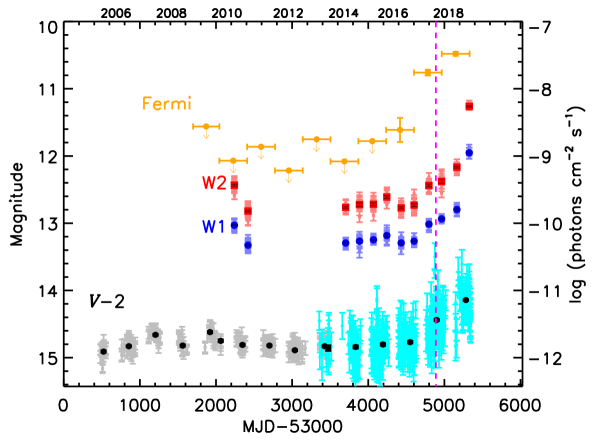
Figure 1: The $\gamma$-ray, optical and MIR light curves of Fermi J1544-0649. The Fermi-LAT $\gamma$-ray photon flux (orange) show an increase in 2017 and 2018 relative to previous years. The $V$-band data are collected from public releases of CRTS (grey) and ASAS-SN (cyan); the MIR data are drawn from WISE database in W1 (blue) and W2 (red). The magenta line indicates MJD 57888 (i.e., 2017 May 15), when Fermi J1544-0649 was discovered and so the Fermi flux seen in the second last data is mostly from thereafter.

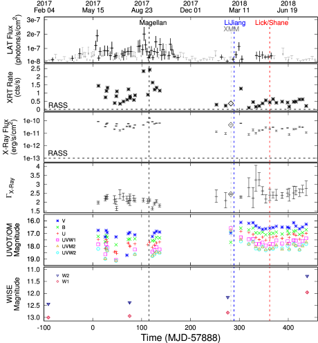
Figure 2: From top to bottom: The Fermi-LAT 0.1-300 GeV photon flux, Swift-XRT 0.3-10 keV count rate, energy flux, photon index, Swift-UVOT magnitudes of various filters, and WISE magnitudes of Fermi J1544-0649 as seen between February 2017 and August 2018. The three arrows in the top panel indicates the dates of spectroscopic observations. When the source is not detected by Fermi-LAT, 90% confidence level upper limits were derived and are plotted in grey. The error bars in the second, fifth and sixth panels are smaller than the symbols. For comparison, the dashed, horizontal lines show the upper limits (a count rate of 0.01 cts/s and an energy flux of $10^{-13}$ erg cm^-2 s^-1) estimated from the RASS observations. A large increase in X-ray flux (up to three orders-of-magnitude) is clearly seen. In the second, third, and fourth panel the black diamonds represent the XMM-EPIC PN result from the 2018 February 21 observation. In the second panel the shown (SWIFT-XRT equivalent) count rate is converted from XMM-EPIC PN count rate with the help of WebPIMMS.

2.2 X-ray Emission

2.2.1 XMM-Newton observation

XMM-Newton DDT observation of Fermi J1544-0649 (obs-id: 0811213301) was performed on 21st February, 2018 (MJD 58170) for about 58 ksec. We used EPIC-PN data for the X-ray analysis, as they have higher sensitivity than EPIC-MOS data. We verify that the MOS data return consistent results as the pn data. The data reduction was performed with the software SAS (version 16.1), using the most updated calibration files (updated on May 2018). The event files were processed using ‘epproc’ with ‘bad’ (e.g., ‘hot’, ‘dead’, ‘flickering’) pixels removed. The periods with high background events were examined and excluded by inspecting the light curves in the energy band 10-12 keV. As the X-rays of Fermi J1544-0649 is bright and the pile-up effect is apparent in the source center, we extracted the source events from an annular region with inner radius of 7.5^′′ and outer radius of 40^′′, using single and double events (PATTERN$\leq$4, FLAG=0). The background events were collected from a source-free circular region of radius 40^′′ within net exposure time of 29.93 ks, and are composed of a total of 165 thousand net source counts in 0.3–10 keV band. We grouped the pn spectra to have at least 25 counts in each bin, and we adopt the $\chi^{2}$ statistic for the spectral fits. The fitted pn spectra are shown in Fig. 3. The spectral analysis were performed using XSPEC(v12.9.1m). The uncertainties are given at 90% confidence levels for one parameter.

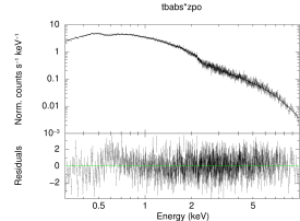
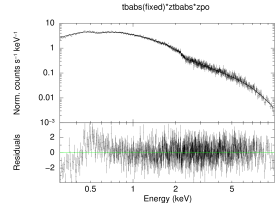
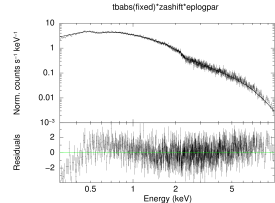
Figure 3: EPIC-pn spectrum fitted with different models for the whole observation

At first, a simple neutral-hydrogen absorbed power-law (PL) model (tbabs $\times$ zpo) was used, and we obtained $\chi^{2}/dof$ = 946/900 with $n_{\rm H}=(14.7\pm 0.27)\times 10^{20}$ cm^-2. To understand the absorption and the spectrum of the object, we compared different models. A simple neutral-hydrogen absorbed PL model (tbabs $\times$ zpo), in which the neutral hydrogen column density is fixed at the Galactic value of $8.98\times 10^{20}$ cm^-2 (Kalberla et al., 2005), is used. It results in $\chi^{2}/dof$ = 2397/901, showing that the model does not work for the data. We then added an intrinsic absorber ($ztbabs$) into the model, where the Redshift is fixed at 0.17 (Chornock and Margutti, 2017). The fit is then much improved ($\chi^{2}/dof$ =1015/900), and results in an intrinsic absorber with neutral hydrogen column density of $(7.0\pm 2.0)\times 10^{20}$ cm^-2. However, there is some systematics in the lowest (0.3–0.8 keV) and highest energy ($>$7 keV). When trying an ionized absorber model (Zdziarski et al., 1995), the ionisation parameter is essentially zero, indicating that the absorber is not heavily ionized.

We have also used a log-parabolic (LP) model ($eplogpar$, in which $N(E)=10^{-b(log(E/E_{\rm p}))^{2}/E^{2}}$ often used for blazars; Tramacere et al., 2007). Here we fix the column density at the Galactic value. We obtained ($\chi^{2}/dof$ = 1121/901) for this model with peak energy $E_{\rm p}=(0.85\pm 0.03)$ keV and a curvature $b$ of $0.40\pm 0.02$. These results are shown in Table. 1. We also tried to allow the column density to vary in the LP model, but the fit parameters are not stable. Based on the above analysis, the PL model (with intrinsic absorption) and the LP model (without intrinsic absorption) can both describe the whole data set well.

Table 1: XMM-Newton EPIC-pn spectral analysis result of Fermi J1544-0649 on 2018 February 21. (I) PL represents tbabs$\times$zpo, (II) PL represents tbabs$\times$ztbabs$\times$zpo and (III) LP represents tbabs$\times$zashift$\times$eplogpar model components.

Models	$n_{\rm H}$(Galactic)	$n_{\rm H}$	$\Gamma$	$E_{\rm p}$	$b$	$10^{11}\times$Flux	$\chi^{2}_{\nu}$
	($10^{22}$ cm-2)	($10^{22}$ cm-2)		(keV)		(erg s-1 cm-2)	(dof)
(I) PL	…	$0.14\pm 0.003$	$2.47\pm 0.01$	…	…	$4.68\pm 0.02$	1.05(900)
(II) PL	0.0898(fixed)	$0.07\pm 0.01$	$2.45\pm 0.01$	…	…	$4.57\pm 0.02$	1.128(900)
(III) LP	0.0898(fixed)	…	…	$0.85\pm 0.03$	$0.40\pm 0.02$	$5.13\pm 0.02$	1.246(901)

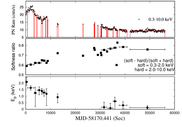
Figure 4: XMM-Newton EPIC-PN cleaned light curve for 0.3–10.0 keV (first panel) energy bands with 100 s time bins and the Bayesian block intervals with 95% statistical significance in red color, along with the softness ratio (second panel) and evolution of the peak energy ($E_{\rm p}$) in the log-parabola model (third panel).

We then looked into the timing analysis. The EPIC-PN cleaned light curve in 0.3–10.0 keV band in 100 s bin is shown in Fig. 4. The background was subtracted and the instrumental effect was corrected using the task ‘epicclorr’. The X-ray light curve shows that Fermi J1544-0649 varies on timescales of a few ks. This prompted us to perform time-resolved spectral analysis. We divided the whole observation into 40 Bayesian blocks (Scargle et al., 2013), calculated with 95% statistical significance using Python module Astropy (Astropy Collaboration et al., 2013, 2018). In Fig. 5 we show the spectra for the two different block intervals. In Fig. 4 top panel blocks are shown with red color along with the cleaned light curve. In the second panel we have calculated the softness ratio between (0.3–2.0) keV and (2.0–10.0) keV energy bands for the Bayesian block intervals. For time resolved spectral analysis we ignored the blocks with lesser number of photons. We used 13 block intervals for time dependent spectral analysis. We employed the PL model (tbabs $\times$ zpo) first. We also used the LP model in the time-resolved spectra. The time-resolved spectral analysis results are shown in Table. 2. It can be seen that the spectrum becomes harder when brighter, i.e., when the count rate decreases, the softness ratio increases and the peak energy (in the LP model) decreases (see, third panel Fig. 4). This shows that the goodness-of-fit (i.e., reduced $\chi^{2}$) in the time-integrated fits is affected by the changing spectrum. To conclude, the PL model is as good as the LP model based on the goodness-of-fit (especially for the short time interval spectral fits). Based on the goodness-of-fit for time-resolved XMM-Newton spectra, we found that the LP model and the PL model can both describe the data well. However, from the broad-band SED, the X-rays represent the synchrotron bump, and it is anticipated that the X-ray spectrum is curved.

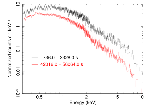
Figure 5: XMM-Newton EPIC-PN cleaned time-resolved spectra for comparison. The color codes represent the time intervals (as defined in Table. 2) as follows: black - 736–3328 sec, red - 42016–56064 sec.

Table 2: XMM-Newton EPIC-PN time-resolved spectral analysis results of Fermi J1544-0649 on 2018 February 21

Model (I): Power law
Interval	$n_{\rm H}$	$\Gamma$	$10^{11}\times Flux$	$\chi^{2}_{\nu}$
(s)	($10^{22}$ cm-2)		(erg s-1 cm-2)	(dof)
0-736	$0.14\pm 0.02$	$2.15\pm 0.07$	$8.12\pm 0.18$	0.85(179)
736-3328	$0.13\pm 0.01$	$2.16\pm 0.03$	$8.55\pm 0.10$	1.17(458)
3424-4320	$0.11\pm 0.02$	$2.12\pm 0.07$	$6.86\pm 0.14$	1.05(196)
4640-6240	$0.13\pm 0.01$	$2.17\pm 0.05$	$6.40\pm 0.11$	0.98(302)
6240-6816	$0.17\pm 0.03$	$2.40\pm 0.11$	$6.06\pm 0.18$	0.96(108)
6816-7936	$0.14\pm 0.02$	$2.27\pm 0.07$	$6.30\pm 0.13$	0.94(208)
8128-8640	$0.14\pm 0.03$	$2.24\pm 0.11$	$6.61\pm 0.19$	1.23(111)
12640-13120	$0.16\pm 0.04$	$2.51\pm 0.15$	$5.10\pm 0.18$	0.94(79)
30624-32512	$0.15\pm 0.04$	$2.66\pm 0.10$	$4.36\pm 0.10$	1.06(166)
33120-35136	$0.13\pm 0.09$	$2.66\pm 0.11$	$3.78\pm 0.09$	0.98(155)
35232-36640	$0.21\pm 0.05$	$2.90\pm 0.15$	$4.91\pm 0.14$	1.34(114)
37632-40832	$0.17\pm 0.04$	$2.83\pm 0.09$	$3.93\pm 0.08$	0.87(210)
42016-56064	$0.14\pm 0.02$	$2.65\pm 0.04$	$3.47\pm 0.03$	1.01(451)
Model (III): Log-parabolic (absorption fixed at the Galactic value)
Interval	$E_{\rm p}$	$b$	$10^{11}\times S_{\rm p}$	$\chi^{2}_{\nu}$
(s)	(keV)		(erg s-1 cm-2)	(dof)
0-736	$2.10\pm 0.31$	$0.32\pm 0.12$	$3.04\pm 0.50$	0.86(179)
736-3328	$1.64\pm 0.17$	$0.24\pm 0.06$	$3.26\pm 0.50$	1.15(458)
3424-4320	$1.26\pm 0.74$	$0.15\pm 0.12$	$2.67\pm 0.50$	1.05(196)
4640-6240	$1.47\pm 0.30$	$0.21\pm 0.09$	$2.44\pm 0.50$	0.98(302)
6240-6816	$1.40\pm 0.22$	$0.53\pm 0.19$	$2.16\pm 0.50$	0.97(108)
6816-7936	$1.28\pm 0.24$	$0.33\pm 0.12$	$2.40\pm 0.50$	0.93(208)
8128-8640	$1.19\pm 0.63$	$0.23\pm 0.18$	$2.49\pm 0.50$	1.26(111)
12640-13120	$0.93\pm 0.34$	$0.49\pm 0.25$	$1.93\pm 0.50$	0.93(79)
35232-36640	$0.62\pm 0.47$	$0.60\pm 0.30$	$1.76\pm 0.51$	1.35(114)

2.2.2 Swift-XRT observations

Since 2017 May 26, Swift monitoring observations have been performed. Here we present all XRT results obtained until 2018 July 25. For Swift-XRT data reduction, the level 2 cleaned event files of SWIFT-XRT were obtained from the events of photon counting (PC) mode data with xrtpipeline. The spectra were extracted from a circular region in the best source position with 20^′′ radius. The background was estimated from an annular region in the same position with radii from 30^′′ to 60^′′. The ancillary response files (arfs) were extracted with xrtmkarf. The PC redistribution matrix file (rmf) version (v.12) was used in the spectral fits. XRT spectra are grouped with 5 counts per bin. XRT spectrum is then analysed with XSPEC(v12.9.1m) in the similar process as the XMM-Newton EPIC-PN spectra. We here fix the absorption column density to be $n_{\rm H}=(14.7\pm 0.27)\times 10^{20}$ cm^-2, the value found from the XMM-Newton analysis. From the fitted spectra, unabsorbed flux values were calculated from 0.3–10 keV in cgs units for all observations. The Swift-XRT light curve and evolution of the power-law index are plotted in Fig. 2. Some but not all Swift spectra can be fitted with the LP model (tbabs*zashift*eplogpar). After the discovery of the first major flare in 2017 May 26, the Swift X-ray light curve shows a second major flaring episode in August and September 2017. After that, the high energy flux has decreased to a lower level, besides a third flaring episode in February to March 2018 (see Fig. 2).

2.2.3 X-ray correlation properties

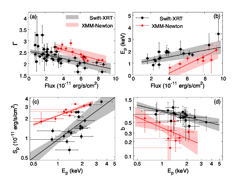
Figure 6: Correlation between model parameters. XMM-Newton time-resolved data are indicated by red diamonds, and Swift data by black circles. (a) Power-law index versus count rate. (b) Peak energy ($E_{\rm p}$) versus count rate. (c) SED peak value ($S_{\rm p}$) versus SED peak energy ($E_{\rm p}$). (d) Spectral curvature $b$ versus peak energy ($E_{\rm p}$).

We perform correlation studies among the flux, PL and LP model parameters to gain insights on the radiation process (see Fig. 6). For all cases linear correlation gives better fit statistics than constant correlation. We calculate Pearson’s Correlation Coefficient (Pearson, 1896) along with standard deviation (Bowley, 1928) for these model parameters using Python module Scipy (Virtanen et al., 2019). In Fig. 6(a), we compare the X-ray flux with the power-law index and find the following relation:

$$for\ {\it XMM-Newton}:$$

$$\Gamma=(-0.11\pm 0.02)\times({\rm flux})+(3.05\pm 0.11)[\chi^{2}_{\nu}=3.09(11)],$$ (2)

$$for\ {\it Swift-XRT}:$$

$$\Gamma=(-0.08\pm 0.01)\times({\rm flux})+(2.55\pm 0.09)[\chi^{2}_{\nu}=1.9(39)].$$ (3)

The correlation coefficient of the X-ray flux and power-law index are $r=-0.86\pm 0.08$ (for XMM-Newton data) and $r=-0.55\pm 0.11$ (Swift data) respectively. These results indicate a harder-when-brighter behavior.

In Fig. 6(b), we compare the X-ray flux with the peak energy. The corresponding correlation coefficient is $r=0.81\pm 0.13$ (for XMM-Newton data) and $r=0.83\pm 0.08$ (Swift data), confirming the harder-when-brighter behavior. Indeed, we find for XMM-Newton and Swift the following relation:

$$for\ {\it XMM-Newton}:$$

$$E_{\rm p}=(0.36\pm 0.05)\times({\rm flux})-(1.30\pm 0.28)[\chi^{2}_{\nu}=1.2(11)],$$ (4)

$$for\ {\it Swift-XRT}:$$

$$E_{\rm p}=(0.14\pm 0.04)\times({\rm flux})+(0.95\pm 0.17)[\chi^{2}_{\nu}=1.0(16)].$$ (5)

Next, we study the relations between the peak energy ($E_{\rm p}$), SED peak value ($S_{\rm p}$) and spectral curvature $b$, in a similar manner as in Tramacere et al. (2007). For XMM-Newton and Swift data, we obtain

$$for\ {\it XMM-Newton}:$$

$$\ln{S_{\rm p}}=(0.46\pm 0.06)*\ln{E_{\rm p}}+(0.77\pm 0.02)[\chi^{2}_{\nu}=0.002(7)],$$ (6)

$$\ln{b}=(-0.73\pm 0.42)*\ln{E_{\rm p}}-(0.95\pm 0.16)[\chi^{2}_{\nu}=0.01(7)],$$ (7)

$$for\ {\it Swift-XRT}:$$

$$\ln{S_{\rm p}}=(0.92\pm 0.19)*\ln{E_{\rm p}}-(0.07\pm 0.13)[\chi^{2}_{\nu}=0.003(16)],$$ (8)

$$\ln{b}=(-0.41\pm 0.14)*\ln{E_{\rm p}}-(0.16\pm 0.07)[\chi^{2}_{\nu}=0.03(16)].$$ (9)

The unit of $S_{\rm p}$ is 10^-11 erg cm^-2 s^-1 and $E_{\rm p}$ is in keV.

The Pearson’s correlation coefficient between $\ln{S_{\rm p}}$ and $\ln{E_{\rm p}}$ is $r=0.86\pm 0.10$ (for XMM-Newton data) and $r=0.71\pm 0.12$ (Swift data), showing strong positive correlation. Within the context of the synchrotron emission from one dominant component, $S_{\rm p}$ depends on $E_{\rm p}$ as: $S_{\rm p}\propto E_{\rm p}^{\alpha}$. The value of $\alpha\sim$0.5–0.9, we find here is smaller than unity, indicating that the spectral change should be caused by variation of the electron average energy ($\alpha=1.5$), or to the magnetic field change ($\alpha=2$), but not due to change in the beaming factor ($\alpha=4$; Tramacere et al., 2007). The result is shown in Fig. 6(c). The correlation between $\ln{b}$ and $\ln{E_{\rm p}}$ is significant ($r=-0.50\pm 0.29$) for XMM-Newton data but not for Swift data ($r=-0.66\pm 0.14$) (with $b\propto E_{\rm p}^{-0.45}$, and such a negative correlation is expected in statistical or stochastic acceleration; Tramacere et al., 2007, one should note that Swift data were taken over a long time span (i.e., more than a year) while the XMM-Newton observation was taken within a day). Therefore, it is plausible that different physics is driving the spectral shape (referring here to the peak energy and curvature) at different time scales. The result is shown in Fig. 6(d).

In summary, owing to the high sensitivity of XMM-Newton, we have found the rapid X-ray variation from Fermi J1544-0649 with timescale down to $\sim$1 hour, and a hardening X-ray spectrum following the rise of the X-ray flux. Both of these findings support a blazar scenario, in which the X-ray emission is dominated by synchrotron emission of a relativistic jet component.

2.2.4 Other X-ray observations

MAXI-GSC 2–20 keV light curve with 1 day time bin was obtained from a circular region at the best source position with 1.6^∘ radius from MAXI online data reduction system. Some excess can be seen in the light curve during and shortly after the two major flares in May and August 2017, respectively.

ROSAT-PSPC observed this position of sky for a total exposure $\sim$480 s during the all-sky survey (RASS). Since there is no detection in this position, and taking 5 counts as a minimum for a detection, the upper limit of the count rate is approximately 0.01. The upper limit of energy flux is taken to be about $10^{-13}$ erg cm^-2 s^-1 (2RXS; Boller et al., 2016). Swift-XRT observations thus revealed a peak X-ray flux more than $10^{3}$ higher than this upper limit. These values are indicated by dashed lines in the XRT count rate and light curve panels in Fig. 2.

3 UV, Optical, and IR properties

3.1 UV and optical photometric measurements

For Swift-UVOT data reduction, all extensions of sky images were stacked with uvotimsum. The source magnitudes were derived with 3-$\sigma$ significance level from the circular region of 5^′′ radius in the best source position of the stacked sky images from all the filters with uvotsource. The background was estimated from an annular region in the same position with radii from 10^′′ to 20^′′. The Swift-UVOT light curves (extinction not corrected) of different filters are plotted in Fig. 2. To check any color change, we also applied interstellar de-reddening on the U, B, and V-magnitudes. The value of extinction was estimated using the web-based calculator maintained by the NASA/IPAC Infrared Science Archive (Schlafly and Finkbeiner, 2011), and the corrected values are shown in Fig. 7. It can be seen that there is no color change against different U-band flux. In particular, no bluer-when-brighter behavior is seen.

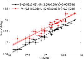
Figure 7: Left: the flux-color plot for optical observations. The x- and y- axis is the U-band magnitude and $B\!-\!V$color index, respectively. Right: B- or V-band magnitude versus U-band magnitude for various optical flux. The black straight line has a slope of $0.83\pm 0.03$, and the red line a slope of $0.81\pm 0.05$. Galactic extinction is corrected for in plotting these figures (see Section. 3.1).

On 2018 February 21, XMM-OM observed Fermi J1544-0649 in FAST mode for 12 exposures with different filters. For XMM-OM data reduction, all exposures of sky images are extracted with omfchain. The source magnitudes are derived with 3-$\sigma$ significance level from the circular region of 5^′′ radius in the best source position of the stacked sky images from all the filters with omdetect. The background is estimated from an annular region in the same position with radii from 10^′′ to 20^′′. The absolute magnitudes obtained from the analysis are shown in Table. 3.

Table 3: XMM-Newton OM analysis results of Fermi J1544-0649 on 2018 February 21

Exposure	Exposure	OM	Absolute
identifier	(s)	Filter	magnitude
S014	4400	V	16.96$\pm$0.02
S015	4400	U	16.86$\pm$0.01
S016	4400	B	17.69$\pm$0.01
S017	4400	B	17.63$\pm$0.01
S018	4400	UVW1	16.57$\pm$0.02
S019	4400	UVW1	16.48$\pm$0.01
S020	4400	UVM2	16.71$\pm$0.04
S021	4400	UVM2	16.80$\pm$0.04
S022	4400	UVM2	16.71$\pm$0.04
S023	4400	UVW2	16.87$\pm$0.07
S024	4400	UVW2	16.75$\pm$0.06
S025	3340	UVW2	16.89$\pm$0.08

In summary, as seen in Fig. 2, the evolution of the optical emission from Fermi J1544-0649 is independent of that of the high-energy (i.e., X/$\gamma$-ray) emission. We did several tests (including a zDCF code Alexander, 1997) and did not find a correlation between $\gamma$-ray or X-ray flux with optical/NIR flux. In particular, the average optical flux in 2018 is higher than that in 2017, but the average X/$\gamma$-ray flux is higher in 2017 than in 2018. This may be due to two emission regions not directly related to each other.

3.2 Long-term Optical and Mid-infrared light curves

A comprehensive examination of the long-term variability of Fermi J1544-0649 in every other available band is helpful for us to understand its nature. We checked its optical and mid-infrared (MIR) light curves as shown in Fig. 1. The optical ($V$-band) data are retrieved from public searching server of Cataline Real-Time Transient Survey (CRTS; Drake et al., 2009) and All-Sky Automated Survey for Supernova (ASAS-SN Shappee et al., 2014; Kochanek et al., 2017). Although with large photometric errors, a long-term variation is clearly visible, indicative of an AGN. After measurement errors are taken into account, the CRTS variability amplitude ($\Delta V$) is $\sim 0.07$ mag (e.g., Equation 6 in Sesar et al., 2007). The ASAS-SN data possess even larger errors due to its shallow survey depth. Despite that, we can still see a significant (i.e., at the 4-$\sigma$ level) brightening in the latest two epochs ($\sim 0.7$ mag).

In addition to the ground-based optical time-domain surveys, the Wide-field Infrared Survey Explorer (WISE Wright et al., 2010; Mainzer et al., 2014) has scanned a specific sky area every half year at 3.4 and 4.6 $\mu$m (labeled W1 and W2) since 2010 Feb (except for a gap between 2011 Feb and 2013 Dec) and thus yielded 12-13 times of observations for each object up to now. We downloaded all of the public WISE data of Fermi J1544-0649 up to the end of 2018 July, distributing over 12 epochs at intervals of half year. For each epoch, there are typically 12 individual exposures within one day. Hence the WISE database allows us to study both its long-term and intra-day MIR variability. First, we binned the data every half year (as we have done in Jiang et al., 2016; Dou et al., 2016), which displays an obvious and continuous trend of brightening since 2017 February. The latest exposures taken in 2018 July has brightened by $\sim$1.3 and $\sim$1.5 magnitudes in W1 and W2, respectively, in comparison with two years earlier; such an increase is even larger than in the optical band. We have also tried to explore the possibility of intra-day variability in each epoch following Jiang et al. (2012); Jiang (2018), which may provide a direct evidence for the jet toward us. Nevertheless, the short-timescale variability is insignificant.

In summary, there are long-term variations in both optical and MIR bands, that are indicators of past AGN activity. Moreover, both bands show a trend of recent brightening, especially in 2018 when the high-energy emission goes down to a lower state.

3.3 Optical spectroscopy

To look for any spectral feature in optical, we obtained three spectra in 2017 and 2018. We carried out an observation using the IMACS (f/2) spectrograph on the 6.5-m Magellan telescope on 2017 September 7, with a total exposure time of 800s. Two standard stars and He–Ne–Ar lamp spectra were taken before and after the exposure for flux and wavelength calibration. The raw two-dimensional data reduction and spectral extraction were accomplished using standard routines in IRAF. To extract the nuclear spectra, we used the APALL task and chose an aperture of 2^′′.

We also performed a spectroscopic observation of Fermi J1544-0649 by the Yunnan Faint Object Spectrograph and Camera (YFOSC) on the 2.4m telescope, located at the Lijiang Station of Yunnan Observatories (longitude = 100^∘01^′51^′′, latitude = 26^∘42^′32^′′N, altitude = 3193 m) of the Chinese Academy of Sciences on 2018 February 28. Grism #14 of YFOSC, which has a resolution of 1.67Å pixel^-1 and wavelength coverage of 3200–7500 Å, was used. Given the seeing conditions, we employed a slit with a width of $2\hbox{$.\!\!^{\prime\prime}$}5$. The total exposure time is 3300 s to achieve a high signal-to-noise (S/N) ratio. The spectroscopic data were reduced following the standard procedures using IRAF, including bias and flat correction, cosmic ray rejection, spectrum extraction, wavelength calibration, and flux calibration. When extracting the spectrum, the aperture was selected to reach 2% of the peak value to include most of the light from the source; a good S/N ratio can therefore be obtained. The emission line of He-Ne lamp was used for wavelength calibration. The aperture of the lamp spectrum was identical to the aperture of the source, ensuring that function between wavelength and the position corresponds to the aperture of the source. BD+33d2642 is used as the spectroscopic standard star to calibrate the flux of the object. Considering the airmass of the standard star and the extinction coefficient at Lijiang Station, the sensitivity function can be determined by using the counts and the flux at each wavelength for the standard star. Then the sensitivity function is applied to Fermi J1544-0649 to convert the counts back to flux for Fermi J1544-0649. The airmass of the object, which is different from the standard star, is also considered.

On 2018 May 11, we obtained a medium resolution (R$\sim$2000) spectrum using the Kast double spectrograph (consisting of red and blue channels) on the 3-m Shane telescope at the Lick Observatory. We used the 600/4310 grism on the blue size and 600/5000 grating on the red side with a wavelength coverage approximately 3300–5500Å and 5500–8000Å. We apply a $1\hbox{$.\!\!^{\prime\prime}$}5$ slit aligned at parallactic angle for the observation with a 30-minute exposure for both channels. The flux calibration is based on the spectrophotometric standard star Feige 67.

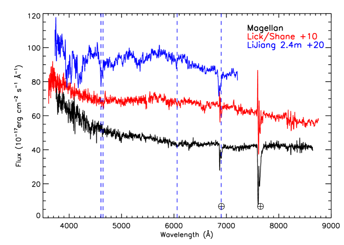
Figure 8: The Lijiang 2.4m spectrum taken on 2018 February 28 (where two possible broad absorption lines (BALs) at around 4000Å and 4200Å are evident), is compared with those taken by the Magellan 6.5m telescope on 2017 September 7 and the Lick-Shane telescope on 2018 May 12. The two crosses mark the position of telluric absorption. Indicated by vertical dashed lines are those of CaII and K, MgI and NaI at z=0.171 (from left to right), but the NaI position is very close to a telluric feature and thus the identification is only tentative. The Magellan spectrum is smoothed by 3 pixels and the Lijiang and Lick-Shane spectrum by 5 pixels for display purpose.

The Magellan and Lick spectra obtained are largely featureless with only weak absorption lines (Fig. 8). These spectra are consistent with Fermi J1544-0649 being a BL Lac object. Along with Lijiang observation, these three optical spectra (taken at times shown by the dashed lines of Fig. 2) has shown strong variation which is not correlated with the X&$\gamma$-ray variation. We also checked that the stellar absorption lines from host galaxy (e.g. CaII, K, MgI and NaI Paiano et al., 2017) in the Lijiang spectrum have a redshift consistent with 0.17 (Chornock and Margutti, 2017; Bruni et al., 2018). The Lijiang spectrum was taken on 2018 February 28.

Surprisingly, in the blue end, there are two unidentified BAL-like features at around 4000 Å and 4200 Å. If it is true, such BAL feature would indicate fast gas outflows blocking the line of sight towards the unknown optical source. This phenomenon is often observed in quasars (Weymann et al., 1991), and has been seen in at least one BL Lac object, PKS B0138-097 (Zhang et al., 2011). Such BAL-like feature does appear just a week after the XMM-OM observation (21 February 2018, MJD 58170) when the optical spectrum (as seen by the magnitudes in different filters) is very blue, as compared to those taken in other epochs (Fig. 2 fifth panel); thus the BAL-like feature is seen during a unique optical color-changing state. The Lijiang observation is performed at the second part of the night before the early morning, sometime, the observation condition changes quickly due to the frog or wet air. However, according to the note by the Lijiang observer, there is no evidence of either quick air change, or instrumental malfunction during the observation time. Fermi J1544-0649 was observed at 2018-02-28 20:41:55.601 for 3300s, and the airmass is 1.359291. The standard star bd332642 was observed at 2018-02-28 20:33:05.119 for 200s, and the AIRMASS is 1.12949. Of course, we could not exclude any undiscovered problems related to the instrument.

4 RATAN 600-meter radio observations

The measurements of the fluxes were obtained with the RATAN-600m radio telescope in transit mode by observing simultaneously at 1.2, 2.3, 4.8, 8.2, 11.2, and 21.7 GHz. The observations were carried out during October and December 2017, and January, February-April and July 2018. The parameters of the antenna and receivers are listed in Table. 4, where $f$ is the central frequency, $\Delta f$ is the bandwidth, $\Delta F$ is the flux density detection limit per beam, and $BW$ – beam width (full width at half-maximum in RA). The detection limit for the RATAN single sector is approximately 5 mJy (the time of integration is 3 s) under good conditions at the frequency of 4.8 GHz and at an average antenna elevation. We averaged the data of observations for 2-25 days in order to get a reliable values of the flux density. Data were reduced using the RATAN standard software FADPS (Flexible Astronomical Data Processing System) reduction package (Verkhodanov, 1997). The flux density measurement procedure is described by Mingaliev et al. (2012, 2014); Udovitskiy et al. (2016); Mingaliev et al. (2017). The following flux density calibrators were applied to obtain the calibration coefficients in the scale by Baars et al. (1977): 3C48, 3C147, 3C161, 3C286 and NGC7027. We also used the traditional RATAN flux density calibrators: J0237$-$23, 3C138, J1154$-$35, and J1347$+$12. Measurements of some calibrators were corrected for linear polarization and angular size, following the data from Ott et al. (1994) and Tabara and Inoue (1980). The systematic uncertainty of the absolute flux scale (3-10% at different RATAN frequencies) is not included in the flux error. The total error in the flux density includes the uncertainty of RATAN calibration curve and the error in the antenna temperature measurement.

Table 4: Parameters of the RATAN-600m antenna and radiometers

$f$	$\Delta$$f$	$\Delta$$F$	FWHMx
GHz	GHz	mJy beam-1	arcsec
$21.7$	$2.5$	$50$	11
$11.2$	$1.4$	$15$	16
$8.2$	$1.0$	$10$	22
$4.8$	$0.6$	$5$	35
$2.25$	$0.08$	$40$	80
$1.28$	$0.08$	$200$	110

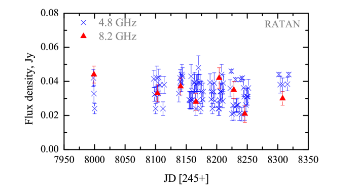
Figure 9: The light curves for Fermi J1544-0649 at 4.8 and 8.2 GHz, obtained by RATAN-600m observations.

The radio emission was detected at 4.8 GHz and 8.2 GHz only. We measured the flux density at 4.8 GHz for each single scan. At the frequency of 8.2 GHz we used all scans in each observation epoch (Fig. 9) to get average flux density. We did not find any significant variation of the flux density in the 2017–2018 measurements. The average flux densities at 4.8 and 8.2 GHz and number of observations in each month are presented in Table. 5.

Table 5: The monthly-average flux densities of Fermi J1544-0649 obtained with the RATAN-600m.

Epoch	$N_{\rm obs}$	$S_{\rm 8.2GHz}$	$S_{\rm 4.8GHz}$
		(Jy)	(Jy)
September 2017
2457998-2458000	3	0.044$\pm$0.005	0.039$\pm$0.002
December 2017
2458097-2458114	11	0.033$\pm$0.005	0.038$\pm$0.003
January 2018
2458138-2458144	6	0.037$\pm$0.005	0.040$\pm$0.002
February 2018
2458155-2458178	21	0.028$\pm$0.005	0.039$\pm$0.002
March 2018
2458189-2458211	16	0.042$\pm$0.006	0.032$\pm$0.002
April 2018
2458222-2458239	11	0.035$\pm$0.005	0.030$\pm$0.002
May 2018
2458240-2458252	10	0.021$\pm$0.005	0.031$\pm$0.002
July 2018
2458302-2458318	5	0.030$\pm$0.004	0.040$\pm$0.003

5 Discussion

5.1 Is Fermi J1544-0649 a blazar?

The most enigmatic behavior of Fermi J1544-0649 is its recent ‘turn-on’ high-energy emission (X-rays and $\gamma$-rays) for about a year, while it remained quiescent for the past decade or so (see Fig. 1). During this ‘turn-on’ state, the $\gamma$-ray flux shows variabilities with a minimum time scale down to weeks. Bruni et al. (2018) suggest that Fermi J1544-0649 is a BL Lac object. Blazars are well known sources that show variability at all time scales from decades down to intra-day (i.e., IDV). And indeed, with XMM-Newton, who has a much better sensitivity than Fermi, we have discovered $<1$ hour variation during a GeV low state.

If Fermi J1544-0649 is a previously unknown blazar, its high-energy flux is constrained to be very low by all-sky monitors like Fermi-LAT and MAXI for around a decade before 2017, as well as ROSAT in the 1990s. The high-energy flares that began in May 2017 thus indicates a high-state never seen before for Fermi J1544-0649. Particularly in $\gamma$-rays, Fermi J1544-0649 remains in the quiescent state for nearly 9 years, which is a rather long period for a Fermi blazar. When comparing the $\gamma$-ray spectrum of Fermi J1544-0649 with sources in the second LAT AGN catalog (2LAC; Ackermann et al., 2011), the mean photon index of the three major categories of $\gamma$-ray BL Lac objects, high-synchrotron-peak (HSP), intermediate-synchrotron-peak, and low-synchrotron-peak, is 1.84, 2.08, and 2.32, respectively. With an average photon index of about 1.7, Fermi J1544-0649 (during its flares) has a spectral index at $\gamma$-rays well within that of HSP BL Lac objects.

In both the low and flaring state, the SED of Fermi J1544-0649 remains a typical blazar SED, which consists mainly of a synchrotron peak in X-rays and an inverse-Compton peak in $\gamma$-rays. During the high state in May 2017, the $\gamma$-ray peak indicates Fermi J1544-0649 to be a high-frequency-peaked BL Lac object. The changing X-ray photon index of Fermi J1544-0649 is around $\Gamma\sim 2.0$ during the major flaring period. i.e., $1.63\pm 0.13$ on MJD 57936, $1.67\pm 0.0.07$ on MJD 57991, and $1.63\pm 0.09$ on MJD 58009, making Fermi J1544-0649 to be an extreme blazar candidate (at times) based on the synchrotron peak frequency (Abdo et al., 2010; Fan et al., 2016). Extreme high-frequency-peaked BL Lac objects (EHBLs), like 1ES 0229+200 and 1ES 1101-232, are blazars with a very high synchrotron peak (c.f., $>$1 keV; Costamante et al., 2001) and usually exhibit exceptionally hard TeV spectra, and they are good probes of the Extra-galactic Background Light (EBL) and Extra-galactic Magnetic Field (EGMF). Yet the sample of extreme blazars remains small (Costamante et al., 2018). Mkn 501 behaved like an EHBL throughout the 2012 observing season, with low and high-energy components peaked above 5 keV and 0.5 TeV, respectively. This suggests that being an EHBL may not be a permanent characteristic of a blazar, but rather a state which may change over time (Pian et al., 1998; Ahnen et al., 2018). Future X-ray/TeV measurements may help us, not just to further probe the synchrotron/IC peak of Fermi J1544-0649, but also to unveil its rapid variations, even during a GeV low state.

5.2 A simple SSC model for this blazar candidate – Fermi J1544-0649

Following the hypothesis that Fermi J1544-0649 is a blazar, we employ a simple Synchrotron Self-Compton (SSC) model to estimate the physics in Fermi J1544-0649. This SSC zone could be either from the main jet in a typical blazar scenario, or from a mini-jet in a misaligned blazar scenario. Since the source is varying by a large factor, spectral energy distribution (SED) are shown for two representative dates: 2017 May 26 (during the first flare) and 2017 July 1 (between the first and second flare), as shown in Fig. 10. It has a broad-band SED consistent with a BL Lac object.

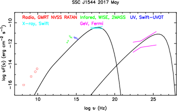
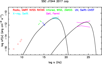
Figure 10: The SED for two representative dates: 2017 May 26 (left panel for the first flare) and 2017 July 1 (right panel, between first and second flare). The model lines are from a one-zone SSC model described in the text. The Fermi spectra were derived from 2017 May 25–27 and 2017 June 30–July 2, respectively. The 4.8 and 8.2 GHz data are from RATAN-600m observations taken in September 2017. Galactic extinction is not corrected for the UV/optical/NIR data shown.

During the SSC fitting of the SED of Fermi J1544-0649, the first constraint comes from the relatively low UV emission when compared to the X-ray emission, clearly the UV emission is supposed to be mainly from the host galaxy and other sources rather than this synchrotron emission, in case of Fermi J1544-0649 it is particularly dominated by an unknown continuum component that varies independent from the X&$\gamma$-ray emission; therefore, the observed UV emission can only serve as an upper limit in our spectrum fitting, and a very hard electron spectral index of $-$1.4 is introduced in both the high state and the low state fittings. Noticeably, the intrinsic UV flux accompanied by the $\gamma-$ray flare could be much higher than this limit, due to the unknown extinction.

With such a hard electron spectrum, the inverse Compton (IC) fitting of the low state requires an electron cutoff energy of a quite low energy (8 GeV in Fig 10), in order to constrain the IC peak at $<$10²⁵ Hz; As a consequence of choosing such a low cutoff energy, a very compact gamma-ray emitting region is needed to boost up the IC flux. In Fig. 10, we adopt a $R_{\rm b}$ size of merely 2.3$\times$10¹⁴ cm in the comoving frame, which corresponds to a minimum GeV variability of 10 minutes when using a Doppler factor of 25 (which is in the range of Doppler factors for blazars, e.g., Savolainen et al., 2010; Fan et al., 2014; Liodakis et al., 2017). As a comparison, the radius of the Innermost Stable Circular Orbit of a $3\times 10^{8}M_{\odot}$ black hole (Bruni et al., 2018) is roughly 2.4$\times$10¹⁴ cm.

The observed GeV spectrum of the high state is very hard and it allows the electron cutoff energy to move freely above 10 GeV during the fitting. This large parameter space of fitting the high state is also due to the lack of direct observational constraints on the magnetic field $B$, Doppler factor $\delta$, and the size of the gamma-ray emitting region $R_{\rm b}$. In Fig. 10, we have shown one of the many fitting results with an electron cutoff energy of 25 GeV. More parameter details about our fitting can be found in Table. 6.

Table 6: Parameters used in the SED fits. Here $E_{\rm e}$ only represents the total electron energy currently in the GeV emitting region, it is a free parameter, meanwhile the total energy output per second for a jet is around 10⁴⁵ erg/s.

Epoch	$B$	$R_{\rm b}$	$\delta$	$p$	$E_{\rm cut}$	$E_{\rm e}$
	(G)	(cm)			(GeV)	(erg)
May 2017	0.4	3$\times$1015	25	$-$1.4	25	2.16$\times$1045
July 2017	3	3.2$\times$1014	25	$-$1.5	8	4.76$\times$1043

5.3 The mysterious optical variation and MIR flare

The strong optical variation of Fermi J1544-0649, as seen in Fig. 2, does not show one-to-one consistency with the X-/$\gamma$-rayvariation. Thus, besides the X/$\gamma$-ray flare component and the host galaxy, alternative sources are likely to dominate the optical band, e.g., other blobs in the jet or even from the core region.

$\gamma$-ray sources in BL Lac objects are normally considered as the relativistic shocks inside the jet. It is well accepted that the jet flow is very likely to be intermittent (Wang and Zhou, 2009). When an injected flow catches up with a slower flow or hits some over-dense medium, a shock is formed. The observed blobs in the jet, as seen in those best observed relativistic jets, e.g., M87 (Owen et al., 1989) and 3C 120 (Casadio et al., 2015), are commonly interpreted as shock waves moving along the jet. In case of an intermittent power injection, the shock could slow down and the opening angle of the beaming emission will be widening, the rise and the decay of an internal shock could naturally cause a variety of light curves based on different viewing angles. Clearly, each shock (knot) of the jet could result different non-thermal emissions, see e.g. the well observed jet of 3C 273 and M87 by HST (Biretta et al., 1999; Bahcall et al., 1995) and Chandra (Wilson and Yang, 2002; Sambruna et al., 2001), which has shown clearly resolved knots along the jet, and their peak energies gradually move from X-ray to optical with increasing distances to the nucleus.

To explain the violent variation of this unknown optical source (with timescale down to 1 week) of Fermi J1544-0649, an intrinsic rise & decay of the accelerator close to the BH could cause the optical flare. Additionally, many magnetic launching models suggests a jet field of helix structure, which is also been supported by the polarization observations (e.g., Gabuzda et al., 2004). In the helical model, strongest emission is obtained when the shock wave reaches the bent regions towards the observer (Gomez et al., 1994). In the case where an alternative blob dominating the optical flare through its synchrotron emission, correlated infrared flares are likely to be observed (which is indeed observed in 2018, Fig. 1).

In our simple SSC model above, the optical observation only functions as an upper-limit. Clearly, one-zone jet models, (see, e.g., Bruni et al., 2018), which includes a relativistic jet with a single emitting zone, an accretion disk, and the host galaxy, will face difficulties to explain the observed UV excess, the strong optical variation and MIR flare seen in 2018.

6 Conclusion and Outlook

The high-energy transient Fermi J1544-0649 is likely due to a sudden energy release (geometrical beaming may play a role as well) of a previously unknown BL Lac object, as first suggested by Bruni et al. (2018) – no high-energy emission was ever seen over the $\sim$9 years’ lifetime of the Fermi satellite (nor by MAXI in X-rays) before April 2017. It is important to understand the mechanism that causes the sudden increase of radiation recently. We argue that a shock-in-jet model combined with viewing angle effects may explain the high-energy flares.

Fermi J1544-0649 displays the typical blazar characteristics including strong X/$\gamma$-ray flares after a decade-long quiescent period, a typical blazar SED, and rapid variations with timescale down to $<$1 hour, The optical flux of Fermi J1544-0649 does not vary at the same time with the X/$\gamma$-ray flux. Thus, besides the X/$\gamma$-ray flare component and the host galaxy, alternative sources are likely to dominate the optical band.

Being a HSP BL Lac object, Fermi J1544-0649 is likely a TeV-emitting blazar, and it shows huge variation in X-rays and $\gamma$-rays. Observing Fermi J1544-0649 by current and/or upcoming Cherenkov Telescope Array, e.g., CTA will tell us about the position of the Compton peak, that in turn will constrain the jet physics. At times being an extreme blazar, it would also be another blazar to probe extreme particle acceleration, EBL, and/or EGMF.

7 Acknowledgments

We thank Nidia Morrell for helping during the Magellan observation, and Da-Hai Yan for useful discussion. PHT is supported by the National Science Foundation of China (NSFC) grants 11633007, 11661161010, and U1731136. JM is supported by the NSFC grants 11673062, the Hundred Talent Program of Chinese Academy of Sciences, the Major Program of Chinese Academy of Sciences (KJZD-EW-M06), and the Oversea Talent Program of Yunnan Province. JHF is supported by NSFC grants 11733001 and U1531245. This work is sponsored (in part) by the Chinese Academy of Sciences (CAS), through a grant to the CAS South America Center for Astronomy (CASSACA) in Santiago, Chile. This research made use of data supplied by the High Energy Astrophysics Science Archive Research Center (HEASARC) at NASA’s Goddard Space Flight Center, and the UK Swift Science Data Centre at the University of Leicester. This publication makes use of data products from the Wide-field Infrared Survey Explorer (WISE), which is a joint project of the UCLA, and JPL/California Institute of Technology, funded by NASA. This publication also makes use of data products from NEOWISE, which is a project of the JPL/California Institute of Technology, funded by the Planetary Science Division of NASA. This work is based on observations obtained with XMM-Newton, an ESA science mission with instruments and contributions directly funded by ESA Member States and NASA. This paper includes data gathered with the 6.5 meter Magellan Telescopes located at Las Campanas Observatory, Chile.

References

- Abdo et al. (2010) Abdo, A.A., Ackermann, M., Agudo, I., Ajello, M., Aller, H.D., Aller, M.F., Angelakis, E., Arkharov, A.A., Axelsson, M., Bach, U., 2010. The Spectral Energy Distribution of Fermi Bright Blazars. ApJ 716, 30–70. doi:10.1088/0004-637X/716/1/30, arXiv:0912.2040.
- Acero et al. (2015) Acero, F., Ackermann, M., Ajello, M., Albert, A., Atwood, W.B., Axelsson, M., Baldini, L., Ballet, J., Barbiellini, G., Bastieri, D., 2015. Fermi Large Area Telescope Third Source Catalog. ApJS 218, 23. doi:10.1088/0067-0049/218/2/23, arXiv:1501.02003.
- Ackermann et al. (2011) Ackermann, M., Ajello, M., Allafort, A., Antolini, E., Atwood, W.B., Axelsson, M., Baldini, L., Ballet, J., Barbiellini, G., Bastieri, D., 2011. The Second Catalog of Active Galactic Nuclei Detected by the Fermi Large Area Telescope. ApJ 743, 171. doi:10.1088/0004-637X/743/2/171, arXiv:1108.1420.
- Ahnen et al. (2018) Ahnen, M.L., Ansoldi, S., Antonelli, L.A., Arcaro, C., Babić, A., Banerjee, B., Bangale, P., Barres de Almeida, U., Barrio, J.A., Becerra González, J., 2018. Extreme HBL behavior of Markarian 501 during 2012. A&A 620, A181. doi:10.1051/0004-6361/201833704, arXiv:1808.04300.
- Alexander (1997) Alexander, T., 1997. Is AGN Variability Correlated with Other AGN Properties? ZDCF Analysis of Small Samples of Sparse Light Curves, in: Maoz, D., Sternberg, A., Leibowitz, E.M. (Eds.), Astronomical Time Series, p. 163. doi:10.1007/978-94-015-8941-3_14.
- Astropy Collaboration et al. (2018) Astropy Collaboration, Price-Whelan, A.M., Sipőcz, B.M., Günther, H.M., Lim, P.L., Crawford, S.M., Conseil, S., Shupe, D.L., Craig, M.W., Dencheva, N., Ginsburg, A., Vand erPlas, J.T., Bradley, L.D., Pérez-Suárez, D., de Val-Borro, M., Aldcroft, T.L., Cruz, K.L., Robitaille, T.P., Tollerud, E.J., Ardelean, C., Babej, T., Bach, Y.P., Bachetti, M., Bakanov, A.V., Bamford, S.P., Barentsen, G., Barmby, P., Baumbach, A., Berry, K.L., Biscani, F., Boquien, M., Bostroem, K.A., Bouma, L.G., Brammer, G.B., Bray, E.M., Breytenbach, H., Buddelmeijer, H., Burke, D.J., Calderone, G., Cano Rodríguez, J.L., Cara, M., Cardoso, J.V.M., Cheedella, S., Copin, Y., Corrales, L., Crichton, D., D’Avella, D., Deil, C., Depagne, É., Dietrich, J.P., Donath, A., Droettboom, M., Earl, N., Erben, T., Fabbro, S., Ferreira, L.A., Finethy, T., Fox, R.T., Garrison, L.H., Gibbons, S.L.J., Goldstein, D.A., Gommers, R., Greco, J.P., Greenfield, P., Groener, A.M., Grollier, F., Hagen, A., Hirst, P., Homeier, D., Horton, A.J., Hosseinzadeh, G., Hu, L., Hunkeler, J.S., Ivezić, Ž., Jain, A., Jenness, T., Kanarek, G., Kendrew, S., Kern, N.S., Kerzendorf, W.E., Khvalko, A., King, J., Kirkby, D., Kulkarni, A.M., Kumar, A., Lee, A., Lenz, D., Littlefair, S.P., Ma, Z., Macleod, D.M., Mastropietro, M., McCully, C., Montagnac, S., Morris, B.M., Mueller, M., Mumford, S.J., Muna, D., Murphy, N.A., Nelson, S., Nguyen, G.H., Ninan, J.P., Nöthe, M., Ogaz, S., Oh, S., Parejko, J.K., Parley, N., Pascual, S., Patil, R., Patil, A.A., Plunkett, A.L., Prochaska, J.X., Rastogi, T., Reddy Janga, V., Sabater, J., Sakurikar, P., Seifert, M., Sherbert, L.E., Sherwood-Taylor, H., Shih, A.Y., Sick, J., Silbiger, M.T., Singanamalla, S., Singer, L.P., Sladen, P.H., Sooley, K.A., Sornarajah, S., Streicher, O., Teuben, P., Thomas, S.W., Tremblay, G.R., Turner, J.E.H., Terrón, V., van Kerkwijk, M.H., de la Vega, A., Watkins, L.L., Weaver, B.A., Whitmore, J.B., Woillez, J., Zabalza, V., Astropy Contributors, 2018. The Astropy Project: Building an Open-science Project and Status of the v2.0 Core Package. AJ 156, 123. doi:10.3847/1538-3881/aabc4f, arXiv:1801.02634.
- Astropy Collaboration et al. (2013) Astropy Collaboration, Robitaille, T.P., Tollerud, E.J., Greenfield, P., Droettboom, M., Bray, E., Aldcroft, T., Davis, M., Ginsburg, A., Price-Whelan, A.M., Kerzendorf, W.E., Conley, A., Crighton, N., Barbary, K., Muna, D., Ferguson, H., Grollier, F., Parikh, M.M., Nair, P.H., Unther, H.M., Deil, C., Woillez, J., Conseil, S., Kramer, R., Turner, J.E.H., Singer, L., Fox, R., Weaver, B.A., Zabalza, V., Edwards, Z.I., Azalee Bostroem, K., Burke, D.J., Casey, A.R., Crawford, S.M., Dencheva, N., Ely, J., Jenness, T., Labrie, K., Lim, P.L., Pierfederici, F., Pontzen, A., Ptak, A., Refsdal, B., Servillat, M., Streicher, O., 2013. Astropy: A community Python package for astronomy. A&A 558, A33. doi:10.1051/0004-6361/201322068, arXiv:1307.6212.
- Atwood et al. (2009) Atwood, W.B., Abdo, A.A., Ackermann, M., Althouse, W., Anderson, B., Axelsson, M., Baldini, L., Ballet, J., Band, D.L., Barbiellini, G., 2009. The Large Area Telescope on the Fermi Gamma-Ray Space Telescope Mission. ApJ 697, 1071–1102. doi:10.1088/0004-637X/697/2/1071, arXiv:0902.1089.
- Baars et al. (1977) Baars, J.W.M., Genzel, R., Pauliny-Toth, I.I.K., Witzel, A., 1977. Reprint of 1977A&A….61…99B. The absolute spectrum of Cas A; an accurate flux density scale and a set of secondary calibrators. A&A 500, 135–142.
- Bahcall et al. (1995) Bahcall, J.N., Kirhakos, S., Schneider, D.P., Davis, R.J., Muxlow, T.W.B., Garrington, S.T., Conway, R.G., Unwin, S.C., 1995. Hubble Space Telescope and MERLIN Observations of the Jet in 3C 273. ApJ 452, L91. doi:10.1086/309717, arXiv:astro-ph/9509028.
- Biretta et al. (1999) Biretta, J.A., Sparks, W.B., Macchetto, F., 1999. Hubble Space Telescope Observations of Superluminal Motion in the M87 Jet. ApJ 520, 621–626. doi:10.1086/307499.
- Boller et al. (2016) Boller, T., Freyberg, M.J., Trümper, J., Haberl, F., Voges, W., Nandra, K., 2016. Second ROSAT all-sky survey (2RXS) source catalogue. A&A 588, A103. doi:10.1051/0004-6361/201525648, arXiv:1609.09244.
- Bowley (1928) Bowley, A.L., 1928. The standard deviation of the correlation coefficient. Journal of the American Statistical Association 23, 31–34. URL: http://www.jstor.org/stable/2277400.
- Bruni et al. (2018) Bruni, G., Panessa, F., Ghisellini, G., Chavushyan, V., Peña-Herazo, H.A., Hernández-García, L., Bazzano, A., Ubertini, P., Kraus, A., 2018. Fermi Transient J1544-0649: A Flaring Radio-weak BL Lac. ApJ 854, L23. doi:10.3847/2041-8213/aaacfb, arXiv:1802.01105.
- Casadio et al. (2015) Casadio, C., Gómez, J.L., Grandi, P., Jorstad, S.G., Marscher, A.P., Lister, M.L., Kovalev, Y.Y., Savolainen, T., Pushkarev, A.B., 2015. The Connection between the Radio Jet and the Gamma-ray Emission in the Radio Galaxy 3C 120. ApJ 808, 162. doi:10.1088/0004-637X/808/2/162, arXiv:1505.03871.
- Chornock and Margutti (2017) Chornock, R., Margutti, R., 2017. MDM Redshift of the Host of ASASSN-17gs. The Astronomer’s Telegram 10491, 1.
- Condon et al. (1998) Condon, J.J., Cotton, W.D., Greisen, E.W., Yin, Q.F., Perley, R.A., Taylor, G.B., Broderick, J.J., 1998. The NRAO VLA Sky Survey. AJ 115, 1693–1716. doi:10.1086/300337.
- Costamante et al. (2018) Costamante, L., Bonnoli, G., Tavecchio, F., Ghisellini, G., Tagliaferri, G., Khangulyan, D., 2018. The NuSTAR view on hard-TeV BL Lacs. MNRAS 477, 4257–4268. doi:10.1093/mnras/sty857, arXiv:1711.06282.
- Costamante et al. (2001) Costamante, L., Ghisellini, G., Giommi, P., Tagliaferri, G., Celotti, A., Chiaberge, M., Fossati, G., Maraschi, L., Tavecchio, F., Treves, A., 2001. Extreme synchrotron BL Lac objects. Stretching the blazar sequence. A&A 371, 512–526. doi:10.1051/0004-6361:20010412, arXiv:astro-ph/0103343.
- Dou et al. (2016) Dou, L., Wang, T.g., Jiang, N., Yang, C., Lyu, J., Zhou, H., 2016. Long Fading Mid-infrared Emission in Transient Coronal Line Emitters: Dust Echo of a Tidal Disruption Flare. ApJ 832, 188. doi:10.3847/0004-637X/832/2/188, arXiv:1605.05145.
- Drake et al. (2009) Drake, A.J., Djorgovski, S.G., Mahabal, A., Beshore, E., Larson, S., Graham, M.J., Williams, R., Christensen, E., Catelan, M., Boattini, A., 2009. First Results from the Catalina Real-Time Transient Survey. ApJ 696, 870–884. doi:10.1088/0004-637X/696/1/870, arXiv:0809.1394.
- Fan et al. (2014) Fan, J.H., Bastieri, D., Yang, J.H., Liu, Y., Hua, T.X., Yuan, Y.H., Wu, D.X., 2014. The lower limit of the Doppler factor for a Fermi blazar sample. Research in Astronomy and Astrophysics 14, 1135–1145. doi:10.1088/1674-4527/14/9/004.
- Fan et al. (2016) Fan, J.H., Yang, J.H., Liu, Y., Luo, G.Y., Lin, C., Yuan, Y.H., Xiao, H.B., Zhou, A.Y., Hua, T.X., Pei, Z.Y., 2016. The Spectral Energy Distributions of Fermi Blazars. ApJS 226, 20. doi:10.3847/0067-0049/226/2/20, arXiv:1608.03958.
- Gabuzda et al. (2004) Gabuzda, D.C., Murray, É., Cronin, P., 2004. Helical magnetic fields associated with the relativistic jets of four BL Lac objects. MNRAS 351, L89–L93. doi:10.1111/j.1365-2966.2004.08037.x, arXiv:astro-ph/0405394.
- Gomez et al. (1994) Gomez, J.L., Alberdi, A., Marcaide, J.M., 1994. Synchrotron emission from bent shocked relativistic jets. II. Shock waves in helical jets. A&A 284, 51–64.
- Heckman and Best (2014) Heckman, T.M., Best, P.N., 2014. The Coevolution of Galaxies and Supermassive Black Holes: Insights from Surveys of the Contemporary Universe. ARA&A 52, 589–660. doi:10.1146/annurev-astro-081913-035722, arXiv:1403.4620.
- Intema et al. (2017) Intema, H.T., Jagannathan, P., Mooley, K.P., Frail, D.A., 2017. The GMRT 150 MHz all-sky radio survey. First alternative data release TGSS ADR1. A&A 598, A78. doi:10.1051/0004-6361/201628536, arXiv:1603.04368.
- Jiang (2018) Jiang, N., 2018. Intraday Mid-infrared Variability of CTA 102 During Its 2016 Giant Outburst. Research Notes of the American Astronomical Society 2, 134. doi:10.3847/2515-5172/aad693.
- Jiang et al. (2016) Jiang, N., Dou, L., Wang, T., Yang, C., Lyu, J., Zhou, H., 2016. The WISE Detection of an Infrared Echo in Tidal Disruption Event ASASSN-14li. ApJ 828, L14. doi:10.3847/2041-8205/828/1/L14, arXiv:1605.04640.
- Jiang et al. (2012) Jiang, N., Zhou, H.Y., Ho, L.C., Yuan, W., Wang, T.G., Dong, X.B., Jiang, P., Ji, T., Tian, Q., 2012. Rapid Infrared Variability of Three Radio-loud Narrow-line Seyfert 1 Galaxies: A View from the Wide-field Infrared Survey Explorer. ApJ 759, L31. doi:10.1088/2041-8205/759/2/L31, arXiv:1210.2800.
- Kalberla et al. (2005) Kalberla, P.M.W., Burton, W.B., Hartmann, D., Arnal, E.M., Bajaja, E., Morras, R., Pöppel, W.G.L., 2005. The Leiden/Argentine/Bonn (LAB) Survey of Galactic HI. Final data release of the combined LDS and IAR surveys with improved stray-radiation corrections. A&A 440, 775–782. doi:10.1051/0004-6361:20041864, arXiv:astro-ph/0504140.
- Kochanek et al. (2017) Kochanek, C.S., Shappee, B.J., Stanek, K.Z., Holoien, T.W.S., Thompson, T.A., Prieto, J.L., Dong, S., Shields, J.V., Will, D., Britt, C., 2017. The All-Sky Automated Survey for Supernovae (ASAS-SN) Light Curve Server v1.0. PASP 129, 104502. doi:10.1088/1538-3873/aa80d9, arXiv:1706.07060.
- Liodakis et al. (2017) Liodakis, I., Marchili, N., Angelakis, E., Fuhrmann, L., Nestoras, I., Myserlis, I., Karamanavis, V., Krichbaum, T.P., Sievers, A., Ungerechts, H., 2017. F-GAMMA: variability Doppler factors of blazars from multiwavelength monitoring. MNRAS 466, 4625–4632. doi:10.1093/mnras/stx002, arXiv:1701.01452.
- Lynden-Bell (1969) Lynden-Bell, D., 1969. Galactic Nuclei as Collapsed Old Quasars. Nature 223, 690–694. doi:10.1038/223690a0.
- Mainzer et al. (2014) Mainzer, A., Bauer, J., Cutri, R.M., Grav, T., Masiero, J., Beck, R., Clarkson, P., Conrow, T., Dailey, J., Eisenhardt, P., 2014. Initial Performance of the NEOWISE Reactivation Mission. ApJ 792, 30. doi:10.1088/0004-637X/792/1/30, arXiv:1406.6025.
- Mingaliev et al. (2017) Mingaliev, M., Sotnikova, Y., Mufakharov, T., Nieppola, E., Tornikoski, M., Tammi, J., Lähteenmäki, A., Udovitskiy, R., Erkenov, A., 2017. Simultaneous spectra and radio properties of BL Lacs. Astronomische Nachrichten 338, 700–714. doi:10.1002/asna.201713361, arXiv:1707.07949.
- Mingaliev et al. (2012) Mingaliev, M.G., Sotnikova, Y.V., Torniainen, I., Tornikoski, M., Udovitskiy, R.Y., 2012. Multifrequency study of GHz-peaked spectrum sources and candidates with the RATAN-600 radio telescope. A&A 544, A25. doi:10.1051/0004-6361/201118506.
- Mingaliev et al. (2014) Mingaliev, M.G., Sotnikova, Y.V., Udovitskiy, R.Y., Mufakharov, T.V., Nieppola, E., Erkenov, A.K., 2014. RATAN-600 multi-frequency data for the BL Lacertae objects. A&A 572, A59. doi:10.1051/0004-6361/201424437, arXiv:1410.2835.
- Ott et al. (1994) Ott, M., Witzel, A., Quirrenbach, A., Krichbaum, T.P., Standke, K.J., Schalinski, C.J., Hummel, C.A., 1994. An updated list of radio flux density calibrators. A&A 284, 331–339.
- Owen et al. (1989) Owen, F.N., Hardee, P.E., Cornwell, T.J., 1989. High-Resolution, High Dynamic Range VLA Images of the M87 Jet at 2 Centimeters. ApJ 340, 698. doi:10.1086/167430.
- Paiano et al. (2017) Paiano, S., Falomo, R., Landoni, M., Treves, A., Scarpa, R., 2017. An optical view of extragalactic gamma-ray emitters. Frontiers in Astronomy and Space Sciences 4, 45. doi:10.3389/fspas.2017.00045, arXiv:1711.00325.
- Pearson (1896) Pearson, K., 1896. Mathematical Contributions to the Theory of Evolution. III. Regression, Heredity, and Panmixia. Philosophical Transactions of the Royal Society of London Series A 187, 253–318. doi:10.1098/rsta.1896.0007.
- Pian et al. (1998) Pian, E., Vacanti, G., Tagliaferri, G., Ghisellini, G., Maraschi, L., Treves, A., Urry, C.M., Fiore, F., Giommi, P., Palazzi, E., 1998. BeppoSAX Observations of Unprecedented Synchrotron Activity in the BL Lacertae Object Markarian 501. ApJ 492, L17–L20. doi:10.1086/311083, arXiv:astro-ph/9710331.
- Sambruna et al. (2001) Sambruna, R.M., Urry, C.M., Tavecchio, F., Maraschi, L., Scarpa, R., Chartas, G., Muxlow, T., 2001. Chandra Observations of the X-Ray Jet of 3C 273. ApJ 549, L161–L165. doi:10.1086/319157, arXiv:astro-ph/0101299.
- Savolainen et al. (2010) Savolainen, T., Homan, D.C., Hovatta, T., Kadler, M., Kovalev, Y.Y., Lister, M.L., Ros, E., Zensus, J.A., 2010. Relativistic beaming and gamma-ray brightness of blazars. A&A 512, A24. doi:10.1051/0004-6361/200913740, arXiv:0911.4924.
- Scargle et al. (2013) Scargle, J.D., Norris, J.P., Jackson, B., Chiang, J., 2013. Studies in Astronomical Time Series Analysis. VI. Bayesian Block Representations. ApJ 764, 167. doi:10.1088/0004-637X/764/2/167, arXiv:1207.5578.
- Schlafly and Finkbeiner (2011) Schlafly, E.F., Finkbeiner, D.P., 2011. Measuring Reddening with Sloan Digital Sky Survey Stellar Spectra and Recalibrating SFD. ApJ 737, 103. doi:10.1088/0004-637X/737/2/103, arXiv:1012.4804.
- Sesar et al. (2007) Sesar, B., Ivezić, Ž., Lupton, R.H., Jurić, M., Gunn, J.E., Knapp, G.R., DeLee, N., Smith, J.A., Miknaitis, G., Lin, H., Tucker, D., Doi, M., Tanaka, M., Fukugita, M., Holtzman, J., Kent, S., Yanny, B., Schlegel, D., Finkbeiner, D., Padmanabhan, N., Rockosi, C.M., Bond, N., Lee, B., Stoughton, C., Jester, S., Harris, H., Harding, P., Brinkmann, J., Schneider, D.P., York, D., Richmond, M.W., Vanden Berk, D., 2007. Exploring the Variable Sky with the Sloan Digital Sky Survey. AJ 134, 2236–2251. doi:10.1086/521819, arXiv:0704.0655.
- Shappee et al. (2014) Shappee, B.J., Prieto, J.L., Grupe, D., Kochanek, C.S., Stanek, K.Z., De Rosa, G., Mathur, S., Zu, Y., Peterson, B.M., Pogge, R.W., 2014. The Man behind the Curtain: X-Rays Drive the UV through NIR Variability in the 2013 Active Galactic Nucleus Outburst in NGC 2617. ApJ 788, 48. doi:10.1088/0004-637X/788/1/48, arXiv:1310.2241.
- Tabara and Inoue (1980) Tabara, H., Inoue, M., 1980. A catalogue of linear polarization of radio sources. A&AS 39, 379–393.
- Tramacere et al. (2007) Tramacere, A., Massaro, F., Cavaliere, A., 2007. Signatures of synchrotron emission and of electron acceleration in the X-ray spectra of Mrk 421. A&A 466, 521–529. doi:10.1051/0004-6361:20066723, arXiv:astro-ph/0702151.
- Udovitskiy et al. (2016) Udovitskiy, R.Y., Sotnikova, Y.V., Mingaliev, M.G., Tsybulev, P.G., Zhekanis, G.V., Nizhelskij, N.A., 2016. Automated system for reduction of observational data on RATAN-600 radio telescope. Astrophysical Bulletin 71, 496–505. doi:10.1134/S1990341316040131.
- Urry and Padovani (1995) Urry, C.M., Padovani, P., 1995. Unified Schemes for Radio-Loud Active Galactic Nuclei. PASP 107, 803. doi:10.1086/133630, arXiv:astro-ph/9506063.
- Verkhodanov (1997) Verkhodanov, O.V., 1997. Multiwave Continuum Data Reduction at RATAN-600, in: Hunt, G., Payne, H. (Eds.), Astronomical Data Analysis Software and Systems VI, p. 46.
- Virtanen et al. (2019) Virtanen, P., Gommers, R., Oliphant, T.E., Haberland, M., Reddy, T., Cournapeau, D., Burovski, E., Peterson, P., Weckesser, W., Bright, J., van der Walt, S.J., Brett, M., Wilson, J., Jarrod Millman, K., Mayorov, N., Nelson, A.R.J., Jones, E., Kern, R., Larson, E., Carey, C., Polat, İ., Feng, Y., Moore, E.W., Vand erPlas, J., Laxalde, D., Perktold, J., Cimrman, R., Henriksen, I., Quintero, E.A., Harris, C.R., Archibald, A.M., Ribeiro, A.H., Pedregosa, F., van Mulbregt, P., Contributors, S…, 2019. SciPy 1.0–Fundamental Algorithms for Scientific Computing in Python. arXiv e-prints , arXiv:1907.10121arXiv:1907.10121.
- Wang and Zhou (2009) Wang, C.C., Zhou, H.Y., 2009. Determination of the intrinsic velocity field in the M87 jet. MNRAS 395, 301–310. doi:10.1111/j.1365-2966.2009.14463.x, arXiv:0904.1857.
- Weymann et al. (1991) Weymann, R.J., Morris, S.L., Foltz, C.B., Hewett, P.C., 1991. Comparisons of the Emission-Line and Continuum Properties of Broad Absorption Line and Normal Quasi-stellar Objects. ApJ 373, 23. doi:10.1086/170020.
- Wilson and Yang (2002) Wilson, A.S., Yang, Y., 2002. Chandra X-Ray Imaging and Spectroscopy of the M87 Jet and Nucleus. ApJ 568, 133–140. doi:10.1086/338887, arXiv:astro-ph/0112097.
- Wright et al. (2010) Wright, E.L., Eisenhardt, P.R.M., Mainzer, A.K., Ressler, M.E., Cutri, R.M., Jarrett, T., Kirkpatrick, J.D., Padgett, D., McMillan, R.S., Skrutskie, M., 2010. The Wide-field Infrared Survey Explorer (WISE): Mission Description and Initial On-orbit Performance. AJ 140, 1868–1881. doi:10.1088/0004-6256/140/6/1868, arXiv:1008.0031.
- Zdziarski et al. (1995) Zdziarski, A.A., Johnson, W.N., Done, C., Smith, D., McNaron-Brown, K., 1995. The Average X-Ray/Gamma-Ray Spectra of Seyfert Galaxies from GINGA and OSSE and the Origin of the Cosmic X-Ray Background. ApJ 438, L63. doi:10.1086/187716.
- Zhang et al. (2011) Zhang, S.H., Wang, H.Y., Zhou, H.Y., Wang, T.G., Jiang, P., 2011. Discovery of a variable broad absorption line in the BL Lac object PKS B0138-097. Research in Astronomy and Astrophysics 11, 1163–1170. doi:10.1088/1674-4527/11/10/005, arXiv:1106.1587.