Quantum Many-Body Physics with Ultracold Polar Molecules: Nanostructured Potential Barriers and Interactions

Abstract

We design dipolar quantum many-body Hamiltonians that will facilitate the realization of exotic quantum phases under current experimental conditions achieved for polar molecules. The main idea is to modulate both single-body potential barriers and two-body dipolar interactions on a spatial scale of tens of nanometers to strongly enhance energy scales and, therefore, relax temperature requirements for observing new quantum phases of engineered many-body systems. We consider and compare two approaches. In the first, nanoscale barriers are generated with standing wave optical light fields exploiting optical nonlinearities. In the second, static electric field gradients in combination with microwave dressing are used to write nanostructured spatial patterns on the induced electric dipole moments, and thus dipolar interactions. We study the formation of inter-layer and interface bound states of molecules in these configurations, and provide detailed estimates for binding energies and expected losses for present experimental setups.

I Introduction

Recent experimental progress with ultracold polar molecules Park et al. (2017); Rvachov et al. (2017); Reichsöllner et al. (2017); Seeßelberg et al. (2018); Petzold et al. (2018); Ciamei et al. (2018); Guo et al. (2018); De Marco et al. (2019); Anderegg et al. (2019); Yang et al. (2020); Blackmore et al. (2018); Yang et al. (2019); Voges et al. (2019); Tobias et al. (2020) opens up unique opportunities to design novel quantum many-body systems Carr et al. (2009); Krems et al. (2009); Baranov et al. (2012); Bohn et al. (2017). Electric dipole moments, induced by external electric fields in the manifold of rotational molecular ground states, give rise to long-range and anisotropic dipolar interactions, which are potentially larger than those realized with magnetic interactions in atomic systems Griesmaier et al. (2005); Aikawa et al. (2012); Lu et al. (2012); de Paz et al. (2013); Aikawa et al. (2014); Naylor et al. (2015); Baier et al. (2016); Chomaz et al. (2018); Tang et al. (2018); Lepoutre et al. (2019); Patscheider et al. (2020); Guo et al. (2019); Tanzi et al. (2019a, b). Thus polar molecules promise the realization of strongly interacting quantum many-body systems, e.g., as Hubbard or spin models in optical lattices with strong nearest-neighbor or long-range interactions Micheli et al. (2006); Capogrosso-Sansone et al. (2010); Gorshkov et al. (2011a, b), or in bilayer systems with strong controllable inter-layer coupling which can be tuned attractive or repulsive Pikovski et al. (2010); Baranov et al. (2011); Potter et al. (2010); Zinner et al. (2012). In an optical lattice, or a bilayer system created with standing wave laser fields, the interaction energy between dipolar particles scales as $E_{{\rm int}}\sim d^{2}/w^{3}$ with $d$ the (induced) dipole moment and $w$ the lattice- or bilayer spacing provided by $w=\lambda/2$ as half the optical wavelength Pikovski et al. (2010); Baranov et al. (2011); Potter et al. (2010); Zinner et al. (2012). However, only polar molecules with the largest electric dipole moments (LiRb $3.99\,\mathrm{D}$ and LiCs $5.39\,\mathrm{D}$) fulfill the promise of large off-site interactions approaching the scale of tens of kHz, comparable or larger than the other relevant energy scales. These interactions can be quantified by the binding energy $E_{B}$ of a pair of molecules in a head-to-tail configuration in a bilayer system formed by a 1D optical lattice with $w=\lambda/2$ (see Fig. 1(a)). In addition, $E_{B}$ must be larger than available temperatures, $E_{B},E_{{\rm int}}\gtrsim k_{\mathrm{B}}T\approx 1\,\mathrm{kHz}\,h$ De Marco et al. (2019). For polar molecules with small electric dipole moments, meeting these requirements can be challenging: For KRb and $w\equiv\lambda/2=250\,\mathrm{nm}$, and assuming $d=0.33\,\mathrm{D}$ (as dipole moment in Debye induced by a DC electric field $12\,\mathrm{kV}/\mathrm{cm}$) implies binding energies less than kHz.

Thus, the design of strongly interacting many-body systems with dipole moments less than a Debye will require, or strongly benefit from going to much smaller distance scales than those provided by the optical wavelength scale Yi et al. (2008); Nascimbene et al. (2015); Anderson et al. (2020). In the present paper we explore various possibilities of designing quantum many-body systems with polar molecules, involving both nanostructured potential barriers and dipolar interactions modulated on the scale of tens of nanometers, where the goal is to enhance relevant energy scales. We do this by exploiting the unique properties offered by polar molecules: This includes the long life-time of the molecular rotational states in the ground state many-fold, and the possibilities of controlling induced electric dipole moments of rotational states.

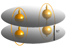
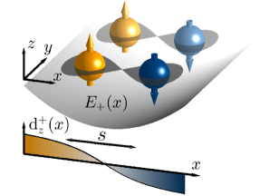
(a) (b)

Figure 1: (a) Polar molecules in a bilayer system in a head-to-tail dipolar configuration attract each other, and can form an inter-layer bound state. Here a nanoscale optical barrier separating the two layers $w\ll\lambda/2$ provides provides strongly enhanced energy scales for the binding energy $E_{B}$ (see Sec. II). (b) Strong electric field gradients allow the induced electric dipole moment of a molecule $\mathrm{d}_{z}^{+}(x)$, to change sign on a short spatial distance scale $s$ (see text). The resulting dipolar interaction allows the formation of interface bound states (see Sec. III).

We will first discuss an all optical scheme (see Sec. II), were following Refs. Ła̧cki et al. (2016); Budich et al. (2017); Lacki et al. (2019); Jendrzejewski et al. (2016); Wang et al. (2018) for atoms, a nanoscale barrier can be realized by exploiting the nonlinear response of a molecule exposed to spatially nonuniform optical light fields in a $\Lambda$-configuration. These nanostructured barriers allow to split a single well in a 1D optical lattice, thus forming a bilayer system with separation on a scale of tens of nanometers. This leads to significant interactions, and inter-layer binding energies even for molecules with comparatively small electric dipole moments. Assuming $w=60\,\mathrm{nm}$, the binding energy becomes $E_{B}>10\,\mathrm{kHz}\,h$ for KRb for an induced dipole moment given above. Table 1 provides a list of interaction and binding energies for various molecules. Besides binding energies, we analyze in detail loss rates expected for this setup, $\Gamma\approx 10^{-2}E_{B}$. For polar molecules there is in addition the opportunity to choose a pair of rotational ground states in the $\Lambda$-system with induced dipole moments having opposite sign. This results in repulsive interactions where one molecule is inside the barrier, i.e.,effectively increasing the barrier height, and a corresponding suppression of the tunneling and thus decay rate. This can be relevant for chemically reactive molecules Krems et al. (2009).

Second, we discuss an all electric scheme (see Sec. III), where instead of the field gradients provided by an optical standing wave we exploit electric field gradients Covey (2018), resulting in position-dependent energy shifts of molecular states. In contrast to the nanoscale optical (single-particle) potential barrier discussed above, our aim is now to modulate the (two-particle) dipolar interaction between molecules on a short distance scale. The underlying mechanism is to couple a pair of rotational states with opposite induced dipole moments $\mathrm{d}_{z}^{(1)}=-\mathrm{d}_{z}^{(2)}$ with resonant microwave fields. The resulting dressed states of this two-level atom acquire position-dependent dipolar moments $\mathrm{d}_{z}^{+}(x)=\mathrm{d}_{z}^{(1)}\leavevmode\nobreak\ \left[(x/s)/\sqrt{1+(x/s)^{2}}\right]$ illustrated in Fig. 1(b), with the spatial scale of the variation set by the electric field gradient. Thus we design a two-body interaction $V(\boldsymbol{\rho}_{1},\boldsymbol{\rho}_{2})=\mathrm{d}_{z}^{+}(x_{1})\mathrm{d}_{z}^{+}(x_{2})/|\boldsymbol{\rho}_{1}-\boldsymbol{\rho}_{2}|^{3}$, where $\rho_{j}=(x_{j},y_{j})$ labels the position of the $j$^th molecule in the $xy$-plane, see Fig. 1(b). Molecules on different sides of the plane $x=0$ will attract each other allowing for the formation an interface bound state. This state is stabilized by the position dependent dipole-dipole interaction which vanishes the molecules approach $x=0$, and become repulsive for molecules on the same side. We find that a bound state occurs above a critical value of dipolar interactions. For molecules with $d>3\,\mathrm{D}$ (as for LiRb and LiCs) this results in binding energies of tens of kHz for electric field gradients $\sim 5\,\mathrm{kV}/(\mathrm{cm}\,\mathrm{mm})$. We note that while also in this scheme achievable binding energies are in principle enhanced by the nanoscale separation of molecules, this enhancement is partially compensated by the reduction of the dipolar moment in the vicinity of the interface and the aforementioned scaling of $E_{\mathrm{int}}$ is not applicable in this case. In Table 2 we summarize binding energies $E_{B}$ for various molecules for typical parameters. This all-electric scheme may also be of interest when the optical manipulation of molecules is not available.

II inter-layer bound states in optical $\boldsymbol{\Lambda}$-systems

We discuss below bilayer systems for polar molecules with layer separation of tens of nanometers (see Fig. 2). Our work builds on earlier proposals Ła̧cki et al. (2016); Jendrzejewski et al. (2016) and experiments Wang et al. (2018) to realize an optical nanoscale barrier in $\Lambda$-systems. In Sec. II.1 we first summarize how molecular $\Lambda$-systems which consist of two rotational levels coupled by a Raman transition can be trapped in a double-layer geometry with sub-optical-wavelength spacing as illustrated in Fig. 2. In Sec. II.2 we give a detailed account of loss channels in such systems, and we identify a hierarchy of scales which ensures the suppression of losses. Finally, in Sec. II.3 we study the formation of inter-layer bound states of molecules.

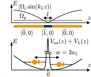
(a) (b) (c)

Figure 2: (a) Raman coupled $\Lambda$-system. The two rotational states $|\widetilde{0},0\rangle$ and $|\widetilde{1},0\rangle$ are coupled by the control and probe laser via the electronically excited state $|e\rangle$. (b) The barrier $V_{\mathrm{na}}(z)$ arises as a nonadiabatic correction to the slow motion of a molecule in the dark-state Born-Oppenheimer channel of a $\Lambda$-system with spatially inhomogeneous Rabi frequencies. The control Rabi beam vanishes at $z=0$ which determines the position of the potential barrier $V_{\mathrm{na}}(z)$. In the lower panel, the dark-state decomposition as a function of position is schematically illustrated. (c) A double well potential for dipolar molecules is created by inserting an optical nanoscale barrier $V_{\mathrm{na}}(z)$ into a single potential well generated by $V_{L}(z)$. In order to split the potential well into two sites, the width $l$ of $V_{L}(z)$ has to be smaller than the ground state size $a_{L}$ of $V_{L}(z)$. The effective separation of the molecules is $w=2a_{L}$.

The model underlying our discussion is a hetero-nuclear diatomic molecule in its electronic ($X^{1}\Sigma^{+}$ for KRb Covey (2018)) and vibrational ground state placed in a strong external electric field. Under such conditions, the Stark effect dominates over the hyperfine interactions (this happens already for electric field strengths of tens of V/cm Aldegunde et al. (2008); Will et al. (2016)) and, omitting the latter, the Hamiltonian for a molecule is given by

$$H_{M}=H_{R}-\mathbf{\hat{d}}\cdot\boldsymbol{\epsilon},$$ (1)

where $H_{R}=\hbar B\hat{N}^{2}$ is the Hamiltonian of a rigid rotor, $B$ the rotational constant and $\hat{N}$ is the orbital angular momentum operator. Further, $\boldsymbol{\epsilon}$ is the external electric field, $\mathbf{\hat{d}}=\mathcal{D}\,\hat{\mathbf{r}}/|\hat{\mathbf{r}}|$ is the dipole moment operator expressed in terms of the position operator $\hat{\mathbf{r}}$, and $\mathcal{D}$ is the permanent molecule frame dipole moment. For $\boldsymbol{\epsilon}=0$, the eigenstates and energies of $H_{M}=H_{R}$ are $|N,m\rangle$ and $E_{N}=\hbar BN\left(N+1\right)$, respectively, where $N=0,1,2,\dotsc$ denotes the angular momentum quantum number, and $m=-N,-N+1,\dotsc,N$ its projection onto the quantization axis. Here and in the following, we choose both the quantization axis and the $z$-coordinate axis along the direction of the electric field $\boldsymbol{\epsilon}=\epsilon\mathbf{e}_{z}$, such that the angular momentum projection quantum number $m$ is conserved. For $\boldsymbol{\epsilon}\neq 0$, we denote the eigenstates of $H_{M}$ by $|\widetilde{N},m\rangle_{\boldsymbol{\epsilon}}$ and the corresponding energy levels $E_{\widetilde{N},m}(\boldsymbol{\epsilon})$ are shown in panel (a) of Fig. 3. Panel (b) depicts the induced dipole moment which is given by the change of the energy with the electric field $\boldsymbol{\epsilon}$, $\mathbf{d}^{\widetilde{N},m}(\boldsymbol{\epsilon})=-\boldsymbol{\nabla}_{\boldsymbol{\epsilon}}E_{\widetilde{N},m}(\boldsymbol{\epsilon})={}_{\boldsymbol{\epsilon}}\langle\widetilde{N},m|\hat{\mathbf{d}}|\widetilde{N},m\rangle_{\boldsymbol{\epsilon}}$. The induced dipole moment is aligned along the electric field, i.e., along the $z$ axis. From this point on, to simplify the notation, we drop the explicit dependency on $\boldsymbol{\epsilon}$ for all quantities.

As mentioned above, for strong electric fields the Stark effect dominates over the hyperfine interactions and, therefore, the nuclear spins become decoupled from the orbital angular momentum. In this case, both $m$ and $m_{1}+m_{2}$, where $m_{1,2}$ is the the nuclear spin projection of the atom $1$ and $2$, respectively, become good quantum numbers Aldegunde et al. (2008); Will et al. (2016). With an additional magnetic field of a few hundred Gauss, the remaining degeneracy among hyperfine states is lifted, making the individual components $m_{1}$ and $m_{2}$ good quantum numbers. We therefore consider the molecules to be in a single hyperfine state, e.g., the hyperfine groundstate $m_{\mathrm{K}}=-4$ and $m_{\mathrm{Rb}}=3/2$ for ⁴⁰K⁸⁷Rb Ospelkaus et al. (2010).

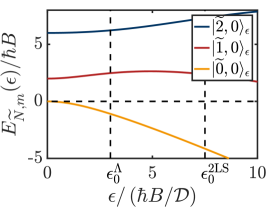
(a)

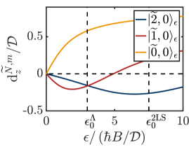
(b)

Figure 3: Energy (a) and induced dipole moment (b) as a function of applied electric field for the lowest energy eigenstates of the molecular Hamiltonian Eq. (1) with $m=0$. $\epsilon^{\Lambda}_{0}$ and $\epsilon^{2\mathrm{LS}}_{0}$ denote the offset fields chosen in Secs. II and III, respectively.

II.1 Summary of nanoscale potentials in optical $\boldsymbol{\Lambda}$-systems

To prepare the ground for the discussion in Secs. II.2 and II.3 and to fix the notation we find it worthwhile for the reader to summarize how to engineer a potential barrier on the nanoscale of size $l$ as proposed in the Refs. Ła̧cki et al. (2016) and Jendrzejewski et al. (2016). The potential barrier is used to cut a single well of an optical potential $V_{L}(z)$ into two sites as illustrated in Fig. 2(c). The optical potential can be approximated in the vicinity of its potential minimum $z_{0}$ by $V_{L}(z)\approx m\omega_{L}^{2}(z-z_{0})^{2}/2$, where $\omega_{L}$ is the harmonic oscillator frequency. The size of the ground state wave function in this potential is $a_{L}=\sqrt{\hbar/(m\omega_{L})}$ and in the limit $l\ll a_{L}$ the potential well is split into two sites. To this end, we consider the motion of a single molecule along the $z$-axis, which is described by

$$H_{\Lambda}=\frac{p_{z}^{2}}{2m}+V_{L}(z)+H_{\Lambda}^{0}(z),$$ (2)

where $p_{z}=-i\hbar\partial_{z}$ is the $z$-component of the momentum operator $\mathbf{p}=-i\hbar\nabla$. For the moment, we consider only the motion along the $z$ axis, and we restore the full 3D form of the Hamiltonian in the next section. $H_{\Lambda}^{0}(z)$ is a position dependent $\Lambda$-system Hamiltonian which is given in a proper rotating frame by

$$H^{0}_{\Lambda}=\hbar\begin{pmatrix}-\Delta&\Omega_{c}(z)/2&\Omega_{p}/2\\ \Omega_{c}(z)/2&0&0\\ \Omega_{p}/2&0&0\end{pmatrix}.$$ (3)

As illustrated in Fig. 2(a), the first leg of the $\Lambda$-system is a weak control laser $\Omega_{p}$ which couples the states $|\widetilde{0},0\rangle$ and an electronically excited state $|e\rangle$; The second leg is a strong standing wave control laser $\Omega_{c}(z)=\Omega_{c}\sin(k_{c}z)$ which couples the states $|\widetilde{1},0\rangle$ and $|e\rangle$. $\Delta$ denotes the detuning of the Raman transition, see Fig. 2(a) and (b). In the case of KRb, a possible candidate for $|e\rangle$ is a vibrational excitation of the $1^{1}\Pi$ electronically excited state Wang et al. (2010), for which the Franck-Condon factor is maximized Okada et al. (1996). Rabi coupling between the state $1^{1}\Pi$ and the absolute ground state of KRb has been demonstrated in Ref. Wang et al. (2010) in the absence of an electric offset field. We discuss the decay of molecules which results from the finite lifetime of the electronically excited state in Sec. II.2.

A Raman coupled $\Lambda$-system always hosts one dark state at zero energy and two bright states, which we denote by $|0\rangle_{z}$ and $|\pm\rangle_{z}$, respectively. The corresponding eigenenergies are given by

$$E^{\Lambda}_{0}=0\mathrm{\leavevmode\nobreak\ and\leavevmode\nobreak\ }E^{\Lambda}_{\pm}=\frac{\hbar}{2}\left[-\Delta\pm\sqrt{\Omega_{p}^{2}+\Omega_{c}^{2}(z)+\Delta^{2}}\right].$$ (4)

and in particular, the dark state reads

$$|0\rangle_{z}=\frac{1}{\sqrt{1+(z/l)^{2}}}\left(z/l|\widetilde{0},0\rangle-|\widetilde{1},0\rangle\right),$$ (5)

where we used that $k_{c}|z-z_{0}|\lesssim k_{c}a_{L}\ll 1$. The characteristic length scale on which the structure of $|0\rangle_{z}$ changes is given by

$$l=\Omega_{p}/(\Omega_{c}\ k_{c}).$$ (6)

For $\lvert z\rvert\gg l$, the dark state is essentially equal to the internal state $|\widetilde{0},0\rangle$; The contribution to $|0\rangle_{z}$ from $|\widetilde{1},0\rangle$ is relevant only in a region of size $l$ around the zero crossing of $\Omega_{c}(z)$ as illustrated in Fig. 2(b).

We consider the limit of slow motion of the molecules, in which the eigenvalues and the eigenstates of $H_{\Lambda}^{0}(z)$ form decoupled Born-Oppenheimer (BO) channels Burrows et al. (2017); Kazantsev et al. (1990); Dum and Olshanii (1996); Dutta et al. (1999); Ruseckas et al. (2005). Nonadiabatic corrections yield two types of contributions: On the one hand, they describes nonadiabatic channel couplings; on the other hand, they gives rise to repulsive potential barriers. Below, we discuss conditions under which the nonadiabatic channel couplings are negligible. Then, the Hamiltonian for the motion of a molecule prepared in the dark state, i.e., the zero-energy channel, can be written as

$$H_{\mathrm{\Lambda},00}^{\mathrm{ad}}=\frac{p_{z}^{2}}{2m}+V_{L}(z)+V_{\mathrm{na}}(z),$$ (7)

where the nonadiabatic potential barrier is independent on the value of $\Delta$ and reads

$$V_{\mathrm{na}}(z)=\frac{\hbar^{2}}{2ml^{2}}\frac{1}{[1+(z/l)^{2}]^{2}},$$ (8)

as introduced in Refs. Ła̧cki et al. (2016) and Jendrzejewski et al. (2016), see also Appendix A.1. The characteristic scale $l$ from Eq. (6), which defines both the width and the height of the potential barrier $V_{\mathrm{na}}(z)$, is determined by the Rabi frequencies $\Omega_{p}$ and $\Omega_{c}$ and the wave vector $k_{c}$, see Fig. 2. By choosing these parameters such that $a_{L}\gg l$, a single potential well generated by $V_{L}(z)$ is split into two sites. This is illustrated in Fig. 4(a), where we show the ground ($\psi_{R}(z)$) and first excited ($\psi_{L}(z)$) state in the zero-energy BO channel, which are located, respectively, to the right and left of the barrier. We obtain the states $\psi_{L,R}(z)$ by numerically diagonalizing the Hamiltonian in Eq. (7). An analytical discussion of the suppression of wave functions inside the barrier is provided in Appendix A.

II.2 Loss channels and hierarchy of scales

The Hamiltonian Eq. (7) ignores nonadiabatic channel couplings. These couplings induce decay of states in the zero-energy BO channel to the other channels. In the vicinity of $z=0$, the energies of the bright states give rise to trapping and antitrapping of molecules in the $+$ and $-$ channels, respectively. Therefore, at low energies, the $+$ channel hosts a discrete set of trapped states. None of these states are resonant with the states $\psi_{L,R}(z)$ in the zero-energy channel if the minimal gap $\hbar\Omega_{p}/2$ between the zero and the $+$ channels is larger than the spacing of levels $\approx\hbar\omega_{L}$ in the zero-energy channel. In contrast, the antitrapped states in the $-$ channel form a continuum, and resonant transitions between the states $\psi_{L,R}(z)$ and states in the $-$ channel are possible. The decay rate from the zero-energy BO channel to the $-$ channel can be obtained by using Fermi’s golden rule. The derivation presented in Appendix A yields for $\Delta=0$

$$\frac{\Gamma_{\Lambda}}{\omega_{L}}=2.5\beta^{2}\frac{l}{a_{L}}\sqrt{\kappa}\leavevmode\nobreak\ \mathrm{exp}\left(-1.75\leavevmode\nobreak\ \kappa\right),$$ (9)

where $\kappa$ is the square root of the ratio of the gap between the zero-energy and $-$ channels and the height of the barrier, $\kappa=(\hbar\Omega_{p}/2)/(\hbar^{2}/2ml^{2})$, and the number $\beta\leq 0.34$ is determined by the exact position of the barrier and the wave function of the trapped state. This result is valid in the limit $\kappa\gg 1$ or equivalently $l/a_{L}\gg\sqrt{\omega_{L}/\Omega_{c}}$, when $\Gamma_{\Lambda}$ is exponentially suppressed. The gap between the zero-energy and $-$ channels and thus the parameter $\kappa$ is enhanced in the far blue-detuned regime in which $\Delta\gg\lvert\Omega_{p,c}\rvert$, and where according to Eq. (4) the size of the gap is equal to $\hbar\Delta$. In this case, Eq. (9) provides only an estimate of the decay rate, because it does not take into account the change of the non-adiabtic couplings with $\Delta$.

In contrast to rotational excitations, electronically excited states have a non-negligible decay rate $\gamma_{e}$. If the motion of molecules in the zero-energy or dark-state channel is perfectly adiabatic, they are not affected by this decay. However, nonadiabatic corrections couple the dark-state channel to the $\pm$ or bright-state channels, and thus lead to a small admixture of the electronically excited state $|e\rangle$ to the dark state, which in turn can lead to inelastic scattering of photons. This effect is strongly suppressed in the far blue-detuned regime: On the one hand, for $\Delta\gg\lvert\Omega_{p,c}\rvert$, the $-$ BO-channel is shifted down energetically, and the mixing between the dark-state and $-$ channels is negligible. On the other hand, the gap between the $+$ and zero-energy channels is reduced. To estimate the mixing between the dark-state and $+$ channels, we first analyze wave functions in the $+$ channel. For $\Delta\gtrsim|\Omega_{p,c}|$ the $+$ bright-state energy in Eq. (4) can be approximated around $z=0$ as a harmonic potential, $E_{+}(z)\approx\Omega_{c}^{2}/(4\Delta)+m\omega_{+}^{2}z^{2}/2$, where $\omega_{+}=\Omega_{c}\sqrt{\hbar^{2}k_{c}^{2}/(2m\Delta)}$ takes the role of the harmonic oscillator frequency. The $+$ channel hosts a barrier which is for far blue detuning equivalent to the one in the zero-energy channel. Therefore, as discussed in Appendix A.2, eigenfunctions in the $+$ channel are suppressed within the barrier by a factor of $l/a_{+}$, where $a_{+}=\sqrt{\hbar/(m\omega_{+})}$ is the oscillator length. The admixture of $+$ channel wave functions can be approximated to first order in the diabatic corrections by $c_{+}\approx(l/a_{L})(l/a_{+})V_{\mathrm{na}}(0)/\Delta E$, where the factors $l/a_{L}$ and $l/a_{+}$ describe the reduction of the dark-state and bright-state wave functions, respectively. The coupling matrix element is approximately given by the height of the barrier $V_{\mathrm{na}}(0)$ Jendrzejewski et al. (2016), and $\Delta E$ is the energy gap. For $\Delta>\Omega_{c}$ the gap o the lowest energy state in the $+$ BO-channel is $\Delta E\approx\hbar\omega_{+}/2$, which yields a relatively small admixture, $|c_{+}|^{2}<0.1$ for $l/a_{L}=0.1$. In the far blue-detuned limit, the amplitude of the excited state $|e\rangle$ in the $+$ channel is small and therefore a reduced decay rate $\gamma_{e}^{+}\approx\gamma_{e}\Omega_{p}^{2}/(8\Delta^{2})$ (see Sec. B2 in the supplementary material of Ref. Ła̧cki et al. (2016)) has to be used to estimate the inelastic scattering rate in the zero-energy BO channel, $\gamma_{e}^{0}\approx\gamma_{e}^{+}|c_{+}|^{2}\approx 10^{-4}\gamma_{e}$, where $\gamma_{e}$ is typically on the order of tens of MHz Wang et al. (2010); Ni et al. (2008). Inelastic light scattering is negligible when $\gamma_{e}^{0}\ll\omega_{L}$, which is indeed the case for $\omega_{L}\approx 2\pi\times 88\,\mathrm{kHz}$ as considered in Sec. II.4.

In addition to the decay of the states $\psi_{L,R}(z)$ in the zero-energy BO channel due to non-adiabatic channel couplings and inelastic light scattering, the stability of a many-body system that is loaded into the states $\psi_{L,R}(z)$ is reduced by inelastic collisions, like chemical reactions Micheli et al. (2010), which can occur at short distances. This effects are minimized when $\psi_{L}(z)$ and $\psi_{R}(z)$ are maximally localized on either side of the barrier. As a measure of the degree of localization we calculate the wave function leakage $\mathcal{O}_{L,R}=\int_{0,-\infty}^{\infty,0}\text{d}z\,\lvert\psi_{L,R}(z)\rvert^{2}$. The leakage is affected by the length scales $a_{L}$, $l$ and $z_{0}$, which determine the shape of the wave functions. For $z_{0}/a_{L}=0.3$, in Fig. 4(c) we observe minimal leakage for a range of small values of $l/a_{L}$. In particular, leakage is negligible in the limit $l/a_{L}\ll 1$.

Even when leakage of the eigenstates of the single-particle Hamiltonian (7) is strongly suppressed, molecules which are loaded into the potential well on one side of the barrier can tunnel through the barrier and collide inelastically with molecules on the other side. Tunneling through the barrier can be estimated by the transmission coefficient $t\approx\sqrt{4E/(\pi^{2}V_{\mathrm{na}}(0))}$ for an incoming plane wave with energy $E\ll V_{\mathrm{na}}(0)$ Lacki et al. (2019). The tunneling rate is then given by $J=t^{2}E/h$, where $t^{2}$ is the probability for a molecule to tunnel through the barrier and $E/h$ is the attempt frequency. For a particle prepared in $\psi_{L,R}(z)$, we set $E=E_{L,R}$, which yields a tunneling constant of $J_{L,R}/\omega_{L}=8/\pi^{3}(l/a_{L})^{2}E_{L,R}^{2}/(\hbar\omega_{L})^{2}$. For a stable bilayer system we require $J_{L,R}/\omega_{L}\ll 1$ which is achievable for $l/a_{L}\ll 1$. In particular, for $l/a_{L}=0.1$ we get $J_{L,R}/\omega_{L}\leq 0.01$.

We obtain a hierarchy of conditions which have to be met by combining the requirements of small leakage, tunneling and decay rates (9):

$$1\gg\frac{l}{a_{L}}\gg\sqrt{\frac{\omega_{L}}{\Omega_{c}}}.$$ (10)

Engineering barriers to cut a single well into two sites is possible if the above states hierarchy of scales is fulfilled. We emphasize that our scheme has sufficiently many “tuning knobs” to adjust each parameter independently. In the next section, we discuss many-body effects arising from dipolar interactions across the barrier.

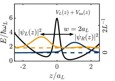
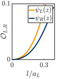
(a) (b)

Figure 4: (a) Spatial probability densities for the ground ($\psi_{R}(z)$) and first excited state ($\psi_{L}(z)$) in the zero-energy BO channel. The dashed baselines indicate the corresponding eigenenergies. The peaks of the wave functions are separated by $w=2a_{L}$. Parameters are $l/a_{L}=0.3$ and $z_{0}/a_{L}=0.3$. Energies and the probability density of $\psi_{R}(z)$ correspond to the left-hand and right-hand axis, respectively, and $L$ denotes the numerical box size. The scale for the probability density of $\psi_{L}(z)$ is the same as for $\psi_{R}(z)$, shifted to the corresponding baseline. (b) Leakage for $\psi_{L}(z)$ and $\psi_{R}(z)$ through the barrier as a function of $l/a_{L}$ with fixed ratio $z_{0}/a_{L}=0.3$.

II.3 Dipolar interaction and inter-layer bound state

We now turn to many-body physics of molecules in the $\Lambda$ configuration discussed above. As an illustrative example, we consider the motion of two identical fermionic molecules. In particular, we study the formation of bound states between molecules on the left and right of the optical nanoscale barrier. We assume a 3D geometry, in which the motion of molecules is not restricted in the $xy$ plane. For molecules in the zero-energy BO channel, the position-dependent internal state is given by $|0\rangle_{z}$ in Eq. (5). The induced dipole moment of this state is oriented along the static electric field, i.e., along the $z$ axis. Therefore, the interaction of molecules within one of the layers $L$ or $R$ is always repulsive not (a), whereas molecules in different layers experience attractive interactions when their separation $\boldsymbol{\rho}=x\mathbf{e}_{x}+y\mathbf{e}_{y}$ in the $xy$ plane has sufficiently small magnitude $\rho=\sqrt{x^{2}+y^{2}}$, so that their relative position corresponds to a head-to-tail configuration. As illustrated in Fig. 1, this can lead to the formation of a bound state.

To describe the bound state quantitatively, we start with the Hamiltonian for the motion of two molecules $j=1,2$ with position coordinates $\mathbf{r}_{j}=(x_{j},y_{j},z_{j})$ in the 3LS configuration described in the previous section, which reads

$$H_{2,\Lambda}=\sum_{j=1,2}\left(\frac{\mathbf{p}_{j}^{2}}{2m}+V_{L}(z_{j})+H^{0}_{\Lambda}(z_{j})\right)$$ (11)

$$+U^{(1)}_{\Lambda}(t)\otimes U^{(2)}_{\Lambda}(t)\leavevmode\nobreak\ V_{\mathrm{dd}}(\mathbf{r}_{1},\mathbf{r}_{2})\leavevmode\nobreak\ U_{\Lambda}^{(2),\dagger}(t)\otimes U_{\Lambda}^{(1),\dagger}(t),$$

where the dipolar interaction is given by

$$V_{\mathrm{dd}}(\mathbf{r})=\frac{1}{|\mathbf{r}|^{3}}\left[\hat{\mathbf{d}}_{1}\cdot\hat{\mathbf{d}}_{2}-3\frac{\hat{\mathbf{d}}_{1}\cdot\mathbf{r}\leavevmode\nobreak\ \hat{\mathbf{d}}_{2}\cdot\mathbf{r}}{|\mathbf{r}|^{2}}\right]$$ (12)

and $U^{(j)}_{\Lambda}(t)=\exp\left[-i\omega_{1}t|\widetilde{0},0\rangle\langle\widetilde{0},0|-i\omega_{2}t|\widetilde{1},0\rangle\langle\widetilde{1},0|\right]$ is the rotating-frame transformation acting on the $j$^th particle. The frequencies $\omega_{1,2}$ are chosen such that $\Delta=\omega_{1}-(E_{e}-E_{\widetilde{0},0})/\hbar=\omega_{2}-(E_{e}-E_{\widetilde{1},0})/\hbar$ where $E_{e}$ denotes the energy of the electronically excited state.

When we project the Hamiltonian in Eq. (11) to the zero-energy channel, the contribution $H_{\Lambda}^{0}(z_{j})$ is replaced by the effective BO potential in Eq. (8). The dipolar interaction for two molecules in the zero-energy BO channel reads

$$\begin{split}V_{\mathrm{dd}}^{0}(\mathbf{r}_{1},\mathbf{r}_{2})=&{}_{z_{1}}\langle 0|\otimes{}_{z_{2}}\langle 0|\left[U^{(1)}_{\Lambda}(t)\otimes U^{(2)}_{\Lambda}(t)\right.\\ \times V_{\mathrm{dd}}(\mathbf{r}_{1},\mathbf{r}_{2})&\leavevmode\nobreak\ \left.U_{\Lambda}^{(2),\dagger}(t)\otimes U_{\Lambda}^{(1),\dagger}(t)\right]|0\rangle_{z_{1}}\otimes|0\rangle_{z_{2}}\\ \approx&\frac{\mathrm{d}_{z}(z_{1})\mathrm{d}_{z}(z_{2})}{r_{1,2}^{3}}\left[1-3\frac{(z_{1}-z_{2})^{2}}{r_{1,2}^{2}}\right],\end{split}$$ (13)

where $r_{1,2}^{2}=(z_{1}-z_{2})^{2}+\rho^{2}$ denotes the relative distance of the two molecules in 3D, and

$$\mathrm{d}_{z}(z)={}_{z}\langle 0|\mathrm{d}_{z}|0\rangle_{z}=\frac{1}{1+(z/l)^{2}}\left[(z/l)^{2}\mathrm{d}^{\widetilde{0},0}_{z}+\mathrm{d}^{\widetilde{1},0}_{z}\right].$$ (14)

The above expression for the dipolar interaction is valid if fast oscillating terms are neglected and the penetration of the single-particle wave functions into the barrier is negligible which is the case for $l/a_{L}\ll 1$. In summary, the projection of the two-molecule Hamiltonian (11) to the zero-energy channel reads

$$H_{2,\Lambda}^{0}=\sum_{j=1,2}\left[\frac{\mathbf{p}_{j}^{2}}{2m}+V_{L}(z_{j})+V_{\mathrm{na}}(z_{j})\right]+V_{\mathrm{dd}}^{0}(\mathbf{r}_{1},\mathbf{r}_{2}).$$ (15)

We assume in the following that the single-particle energy scales associated with the nanoscale potential are dominant as compared to the dipolar interaction, such that motion of the two molecules in the regime of low energies is restricted to the states $\psi_{L}(z)$ and $\psi_{R}(z)$. Under these conditions, the nanoscale potential effectively implements a two-layer geometry, with layers $L$ and $R$ which are parallel to the $xy$ plane. As illustrated in Fig. 4(a), the separation of the peaks of the wave functions defines an effective layer separation given by $w\approx 2a_{L}$. The two-body wave function $\Psi(\mathbf{r}_{1},\mathbf{r}_{2})$ in the zero-energy channel can then be written as

$$\Psi(\mathbf{r}_{1},\mathbf{r}_{2})=\Psi_{\parallel}(\boldsymbol{\rho}_{1},\boldsymbol{\rho}_{2})\sum_{\alpha,\beta=L,R}c_{\alpha\beta}\,\psi_{\alpha}(z_{1})\,\psi_{\beta}(z_{2}).$$ (16)

The component $\Psi_{\parallel}(\boldsymbol{\rho}_{1},\boldsymbol{\rho}_{2})$, which describes motion in the $xy$ plane, can be decomposed further: First, the system is translationally invariant, and therefore $\Psi_{\parallel}(\boldsymbol{\rho}_{1},\boldsymbol{\rho}_{2})=\Psi_{\mathrm{rel}}(\boldsymbol{\rho})\Psi_{\mathrm{COM}}(\mathbf{R})$ factors into contributions corresponding to the relative and COM motion with respective coordinates $\boldsymbol{\rho}=\boldsymbol{\rho}_{1}-\boldsymbol{\rho}_{2}$ and $\mathbf{R}=(\boldsymbol{\rho}_{1}+\boldsymbol{\rho}_{2})/2$. Second, due to the symmetry of the Hamiltonian under rotations around the $z$ axis, the wave function corresponding to the relative motion can be decomposed into radial and angular components, $\Psi_{\mathrm{rel}}(\boldsymbol{\rho})=\sum_{m_{z}\in\mathbb{Z}}\chi_{m_{z}}(\rho)e^{im_{z}\phi}$. To find a bound state it is sufficient to consider $m_{z}=0$, since a nonvanishing angular momentum adds an additional repulsive centrifugal barrier, which increases the energy. Then, antisymmetry of the wave function $\Psi(\mathbf{r}_{1},\mathbf{r}_{2})$ under the exchange of particles requires that the motional state of the two molecules along the $z$ axis is an antisymmetric superposition of the single-particle states $\psi_{L}(z)$ and $\psi_{R}(z)$, that is, the coefficients $c_{\alpha\beta}$ in Eq. (16) are given by $c_{LL}=c_{RR}=0$ and $c_{LR}=-c_{RL}=1/\sqrt{2}$, so that

$$\Psi(\mathbf{r}_{1},\mathbf{r}_{2})=\frac{1}{\sqrt{2}}\chi_{0}(\rho)\Psi_{\mathrm{COM}}(\mathbf{R})\\ \times\left[\psi_{L}(z_{1})\psi_{R}(z_{2})-\psi_{R}(z_{1})\psi_{L}(z_{2})\right].$$ (17)

With this ansatz, the Hamiltonian (11) yields the following Schrödinger equation (SE) for the radial component of the two-body wave function:

$$\left[-\frac{\hbar^{2}}{2m}\left(\frac{\partial^{2}}{\partial\rho^{2}}+\frac{1}{\rho}\frac{\partial}{\partial\rho}\right)+V_{\mathrm{2D}}(\rho)\right]\chi_{0}(\rho)=E_{B}\chi_{0}(\rho).$$ (18)

The effective 2D dipolar interaction is given by

$$V_{\mathrm{2D}}(\rho)=\frac{1}{2}\int\mathrm{d}z_{1}\mathrm{d}z_{2}\leavevmode\nobreak\ V_{\mathrm{dd}}^{0}(\mathbf{r}_{1},\mathbf{r}_{2})\\ \times\left[\psi_{L}(z_{1})\psi_{R}(z_{2})-\psi_{R}(z_{1})\psi_{L}(z_{2})\right]^{2}.$$ (19)

It can be decomposed into “direct” and “exchange” contributions, $V_{\mathrm{2D}}(\rho)=V_{\mathrm{2D}}^{\mathrm{D}}(\rho)-V_{\mathrm{2D}}^{\mathrm{E}}(\rho)$, which read

$$V^{\mathrm{D,E}}_{\mathrm{2D}}(\rho)=\int\mathrm{d}z_{1}\mathrm{d}z_{2}\,\psi_{L,L}(z_{1})\psi_{R,R}(z_{2})\\ \times V_{\mathrm{dd}}(\rho,z_{1},z_{2})\leavevmode\nobreak\ \psi_{R,L}(z_{2})\psi_{L,R}(z_{1}),$$ (20)

In the limit of small spatial wave function overlap which is realized for $l/a_{L}\ll 1$, the exchange part of the interaction gives a strongly suppressed repulsive contribution which we neglect in the following.

A solution to Eq. (18) with $E_{B}<0$ corresponds to a bound state. In Fig. 5(a) and (b), respectively, we show the bound state energy $E_{B}$ and the corresponding wave function for different values of the dipolar length $a^{\widetilde{0},0}_{d}=m\,(\mathrm{d}_{z}^{\widetilde{0},0}/\hbar)^{2}$. We note that the dipolar length scales as $a_{d}^{\widetilde{0},0}/a_{L}\propto\mathcal{D}^{2}m$ with a prefactor which depends on $l/a_{L}$ and $\epsilon_{0}$. The dependence on $\epsilon_{0}$ gives an experimental handle to tune the value of the dipolar length.

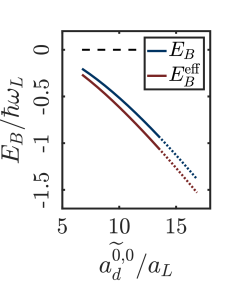
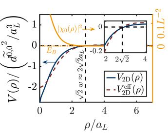
(a) (b)

Figure 5: (a) Energy and effective energy of the inter-layer bound state as a function of the dipolar length $a^{\widetilde{0},0}_{d}$ for $\epsilon_{0}=3\hbar B/\mathcal{D}$ and $l/a_{L}=0.1$. The dotted lines indicate that the results for $\lvert E_{B}\rvert>\hbar\omega_{L}$ should be interpreted as order-of-magnitude estimates. For these values of $E_{B}$, excited single-particle levels, which we neglect in our analysis, begin to contribute to the bound state. (b) Comparision of the interaction potentials $V_{\mathrm{2D}}(\rho)$ and $V^{\mathrm{eff}}_{\mathrm{2D}}(\rho)$. As shown in the inset, both potentials change sign at $\sqrt{2}\leavevmode\nobreak\ w\approx\sqrt{2}\leavevmode\nobreak\ 2a_{L}$. The orange solid line is the radial probability density for the bound state $\chi_{0}(\rho)$, and the dashed baseline indicates the corresponding binding energy. Parameters are the same as in (a) at $a_{d}^{\widetilde{0},0}/{a_{L}=6.9}$. $L$ denotes the numerical box size.

II.4 Experimental parameters

	$\frac{m}{\mathrm{u}}$	$\frac{\mathcal{D}}{\mathrm{Debye}}$	$\frac{\hbar B}{h\,\mathrm{GHz}}$	$\frac{\epsilon_{0}}{\mathrm{kV}/\mathrm{cm}}$	$\frac{a^{\widetilde{0},0}_{d}}{a_{L}}$	$\frac{\lvert E_{B}\rvert}{h\,\mathrm{kHz}}$	$\frac{\lvert E^{\lambda/2}_{B}\rvert}{h\,\mathrm{kHz}}$
KRbDe Marco et al. (2019)	$127$	$0.57$	$1.11$	$11.6$	$6.9$	$17.6$	$<0.1$
Toy	$100$	$1.00$	$1.00$	6.0	$16.8$	$78^{*}$	$0.2$
NaKPark et al. (2015); Voges et al. (2019)	$63$	$2.72$	$2.83$	$6.2$	$78$	$>10^{3^{*}}$	$19$
LiRb	$91$	$3.99$	$7.61$	$11.4$	$242$	$>10^{3^{*}}$	$62$
LiCs	$139$	$5.39$	$6.54$	$7.23$	$676$	$>10^{4^{*}}$	$139^{*}$

Table 1: Parameters for a variety of experimentally relevant fermionic polar molecules Żuchowski et al. (2013); Aymar and Dulieu (2005). For all molecular species, the offset field is chosen as $\epsilon_{0}=3.0\,\hbar B/\mathcal{D}$, which implies $\mathrm{d}_{z}^{\widetilde{0},0}=0.58\mathcal{D}$, $a_{L}=30\,\mathrm{nm}$ and $l/a_{L}=0.1$. The last column presents the binding energy $E_{B}^{\lambda/2}$ achievable for a conventional bilayer-stem with inter layer separation $w=\lambda/2=250\,\mathrm{nm}$ and an electric offset field of $\epsilon_{0}=3.0\,\hbar B/\mathcal{D}$. The asterisk ^∗ marks binding energies which exceed the single-particle level spacing in the potential well, $\lvert E_{B}\rvert>\hbar\omega_{L}$, and thus go beyond the range of validity of our analysis which assumes that the molecules populate only the two lowest-energy single-particle states. Therefore, these values of $E_{B}$ should be considered as order-of-magnitude estimates.

In this section we present experimental parameters for the creation of a bilayer system separated on the nanoscale. As a generic example, we consider KRb De Marco et al. (2019) with mass $m=127\,\mathrm{u}$ and permanent molecule-frame dipole moment $\mathcal{D}=0.57\,\mathrm{Debye}$. We choose the offset field $\epsilon_{0}=3\,\mathrm{\hbar B/\mathcal{D}}$, which implies $\mathrm{d}_{z}^{\widetilde{0},{0}}=0.58\,\mathcal{D}=0.33\,\mathrm{Debye}$ and $a_{d}^{\widetilde{0},0}=207\,\mathrm{nm}$. For $l/a_{L}=0.1$, $z_{0}/a_{L}=0.3$ and an harmonic oscillator length of $a_{L}=30\,\mathrm{nm}$ the binding energy is $\lvert E_{B}\rvert=2\pi\times 18\,\mathrm{kHz}\,\hbar$, well beyond typical temperatures of $50\,\mathrm{nK}\,k_{\mathrm{B}}=2\pi\times 1\,\mathrm{kHz}\,\hbar$ De Marco et al. (2019). In Table 1 binding energies for different polar molecules are summarized.

From a single-particle point of view, we have to fulfill the hierarchy of scales $1\gg l/a_{L}\gg\sqrt{\omega_{L}/\Omega_{c}}$ from Eq. (10). The first inequality ensures that the nonadiabatic barrier splits a single potential well into two sides; The second inequality guarantees stability against nonadiabatic channel couplings, i.e., $\Gamma_{\Lambda}/\omega_{L}\ll 1$, see Eq. (9). To fulfill the hierarchy of scales we choose $\Omega_{p}=100\,\omega_{L}$ which leads to $\Gamma_{\Lambda}/\omega_{L}<4\times 10^{-3}$. For the sake of self-consistency we require $\Gamma_{\Lambda}<\lvert E_{B}\rvert=0.20\,\omega_{L}$. In absolute numbers, the Rabi frequencies are given by $\Omega_{p}=2\pi\times 8.8\,\mathrm{MHz}$ and $\Omega_{c}=2\pi\times 330\,\mathrm{MHz}$, where we used $\lambda_{c}=660\,\mathrm{nm}$ Wang et al. (2010). To ensure single-level addressability of rigid rotor eigenlevels it is necessary to have $\Omega_{c}<B=2\pi\times 1.1\,\mathrm{GHz}$ for KRb.

We note that with the chosen opposite dipole moments ($\mathrm{d}_{z}^{\widetilde{0},0}\approx-\mathrm{d}_{z}^{\widetilde{1},0}/4$) for the dark state constitutes, the interparticle interaction effectively increases the height of the barrier because of the head-to-head or tail-to-tail orientation of the dipole moments when one of the molecule is under the barrier and the other not. The resulting repulsive dipole-dipole interaction $V$ adds to the barrier potential and, hence, suppresses the wave function amplitude under the barrier and, therefore, the tunneling $J_{L,R}$ and $\Gamma_{\Lambda}$. The interaction $V$ can be estimated as $V\approx 2\mathrm{d}_{z}^{\widetilde{0},{0}}\mathrm{d}_{z}^{\widetilde{1},{0}}/a_{L}^{3}\approx 2\pi\times 300\,\mathrm{kHz}\,\hbar$ for the case of KRb, which is $\approx 0.1\,V_{\mathrm{na}}(0)$. This reduces approximately $J_{L,R}$ by $10\%$ and $\Gamma_{\Lambda}$ by $5\%$.

We finally compare achievable binding energies for bilayer systems separated by nanoscale potential barriers to those that can be realized with standard optical lattices. To do so, we define an effective layer separation as follows: The interaction potential for dipolar particles which are held fixed at a relative separation $w$ along the $z$ axis is given by Baranov et al. (2011)

$$V_{\mathrm{2D}}^{\mathrm{eff}}(\rho)={\mathrm{d}_{z}^{\widetilde{0},0}}^{2}\frac{\rho^{2}-2w^{2}}{(\rho^{2}+w^{2})^{5/2}},$$ (21)

and it changes sign at $\rho=\sqrt{2}w$. As illustrated in Fig. 5(b), also the effective dipolar interaction $V_{\mathrm{2D}}(\rho)$ in Eq. (19) exhibits a sign change at $\rho\approx\sqrt{2}2a_{L}$, and we are thus led to identify the effective layer separation as $w=2a_{L}$. Deviations of $V_{\mathrm{2D}}(\rho)$ from the form given in Eq. (21) are most prominent at small separations $\rho$, where $V_{\mathrm{2D}}(\rho)$ exhibits a logarithmic divergence due to the nonvanishing overlap of $\psi_{L}(z)$ and $\psi_{R}(z)$. Nevertheless, the direct comparison in Fig. 5(a) shows good quantitative agreement of the binding energies $E_{B}$ and $E_{B}^{\mathrm{eff}}$ which we obtain for $V_{\mathrm{2D}}(\rho)$ and $V_{\mathrm{2D}}^{\mathrm{eff}}(\rho)$, respectively.

In conventional bilayer systems which are generated with optical lattices, the layers are separated by $\lambda/2$, where $\lambda$ is the optical wavelength Baranov et al. (2011). The inter-layer interaction is then described by the effective potential $V_{\mathrm{2D}}^{\mathrm{eff}}(\rho)$ in Eq. (21), where $w$ is given by $\lambda/2$. This should be compared to the value $w=2a_{L}$ which we obtained above for the nanoscale potential barrier. For $a_{d}^{\widetilde{0},0}/w\gg 1$, the corresponding binding energies can be estimated as $E_{B}^{w}\approx 2a^{\widetilde{0},0}_{d}\hbar^{2}/(mw^{3})$ Baranov et al. (2011). Therefore, reducing the effective layer spacing $w$ from $w=\lambda/2\gtrsim 250\ \mathrm{nm}$ to achievable harmonic oscillator lengths of $w=2a_{L}=60-120\,\mathrm{nm}$ increases the binding energy by 1-2 orders of magnitude. Results for a variety of experimentally relevant molecular species are summarized in Table 1.

III Interface bound state of molecules in electric gradient fields

We now consider the setup illustrated in Fig. 1, in which the electric field gradient created by a standing optical wave is replaced by a static electric gradient field. Further, in contrast to the $\Lambda$-systems with optical transitions which we considered in the previous section, we focus now on effective two-level systems, which are formed by two rotational levels that are coupled by MW fields. As we show, in the adiabatic limit, when the single-particle dynamics occurs in a single BO channel, bound states of two molecules can form at the interface at which the induced dipole moment changes sign.

III.1 Single-particle physics

The key elements to engineer interface bound states are a position-dependent electric field, $\boldsymbol{\epsilon}(x)=\boldsymbol{\epsilon}_{0}+\boldsymbol{\epsilon}^{\prime}x$, which comprises both a homogeneous offset field $\boldsymbol{\epsilon}_{0}$ as discussed at the beginning of Sec. II and a gradient field $\boldsymbol{\epsilon}^{\prime}x=\epsilon^{\prime}\mathbf{e}_{z}x$, and a MW-induced Rabi coupling $\Omega$ of the molecular levels $|\widetilde{0},0\rangle$ and $|\widetilde{2},0\rangle$, see Fig. 6(a) and (b). Note, that these states can be coupled by MW field because of the admixture of the state $|1,0\rangle$ in both of them for $\epsilon_{0}\neq 0$. The reason for the choice of these internal states will be clarified below. As illustrated in Fig. 3(b), the strong offset field $\boldsymbol{\epsilon}_{0}$ induces state-dependent dipole moments $\mathbf{d}^{\widetilde{N},m}$, which couple to the gradient field $\boldsymbol{\epsilon}^{\prime}x$ and thus give rise to position-dependent Stark shifts. To calculate these Stark shifts, we note that in the present setup the motion of the molecules along the $x$-direction is restricted to a region of spatial extent $l_{0}$ which we determine below to be on the order of tens of nanometers, and we assume $\epsilon_{0}\gg\epsilon^{\prime}l_{0}$, so that the gradient field can be taken into account perturbatively. Then, to first order in the gradient field, the Stark shift of the rotational energy levels is $E_{\widetilde{N},m}[\boldsymbol{\epsilon}_{0}+\boldsymbol{\epsilon}^{\prime}x]\approx E_{\widetilde{N},m}(\boldsymbol{\epsilon}_{0})-[\mathbf{d}^{\widetilde{N},m}(\boldsymbol{\epsilon}_{0})\cdot\boldsymbol{\epsilon}^{\prime}]\,x$. To simplify the notation, we omit the dependency on $\boldsymbol{\epsilon}_{0}$ in the following. Higher orders in the expansion in $\boldsymbol{\epsilon}^{\prime}x$ are negligible for the large electric offset fields considered in the following sections. As a result, the molecules move in a state-dependent linear potential, and the Rabi coupling between the internal states is resonant only at a particular point, which we chose as the coordinate origin. The Hamiltonian which describes the motion of a single molecule in this configuration of electric and MW fields is given by

$$H_{\mathrm{2LS}}=\frac{p_{x}^{2}}{2m}+H_{\mathrm{2LS}}^{0}(x),$$ (22)

where $p_{x}=-i\hbar\partial_{x}$ is the $x$-component of the momentum operator. In a proper rotating frame, the MW coupling Hamiltonian reads

$$H_{\mathrm{2LS}}^{0}(x)=\hbar\begin{pmatrix}-\Delta_{\widetilde{2},0}(x)&\Omega/2\\ \Omega/2&-\Delta_{\widetilde{0},0}(x)\end{pmatrix},$$ (23)

with linearly position-dependent detunings, $\Delta_{\widetilde{N},0}(x)=\Delta_{\widetilde{N},0}^{\prime}x$, where $\Delta_{\widetilde{N},0}^{\prime}=-\mathbf{d}^{\widetilde{N},0}\cdot\boldsymbol{\epsilon}^{\prime}/\hbar$. Due to its dependence on the position $x$, the Hamiltonian $H_{\mathrm{2LS}}^{0}(x)$ couples internal and external degrees of freedom. Typically, the energy scales associated with the internal degrees of freedom are much larger than those which characterize the motion of molecules. This allows us to treat the internal dynamics in a BO approximation. To wit, we first diagonalize the 2LS Hamiltonian (23); Thereby, we treat the position $x$ as a parameter. The eigenvalues $E^{\mathrm{2LS}}_{\pm}(x)$ of $H^{0}_{\mathrm{2LS}}(x)$ are given by

$$E^{\mathrm{2LS}}_{\pm}(x)=\frac{\hbar\Omega}{2}\left[\frac{1-\delta}{1+\delta}\frac{x}{s}\pm\sqrt{1+\left(x/s\right)^{2}}\right],$$ (24)

as illustrated in Fig. 6(c), where $-\delta=\Delta^{\prime}_{\widetilde{0},0}/\Delta^{\prime}_{\widetilde{2},0}=\mathrm{d}^{\widetilde{0},0}_{z}/\mathrm{d}^{\widetilde{2},0}_{z}$ is the ratio of induced dipole moments in the states $|\widetilde{0},0\rangle$ and $|\widetilde{2},0\rangle$, and

$$s=\frac{\Omega}{\Delta^{\prime}_{\widetilde{2},0}(1+\delta)}$$ (25)

corresponds to the length scale which delimits the spatial region in which the Rabi coupling is resonant. The corresponding eigenvectors read

$$\begin{split}|+\rangle_{x}&=\sin(\theta_{x}/2)|\widetilde{2},0\rangle+\cos(\theta_{x}/2)|\widetilde{0},0\rangle,\\ |-\rangle_{x}&=\cos(\theta_{x}/2)|\widetilde{2},0\rangle-\sin(\theta_{x}/2)|\widetilde{0},0\rangle,\end{split}$$ (26)

where $\theta_{x}=\mathrm{atan}(s/x)$ and $0\leq\theta_{x}\leq\pi$. The states $|\pm\rangle_{x}$ are superpositions of the rotational states $|\widetilde{0},0\rangle$ and $|\widetilde{2},0\rangle$ with spatially varying amplitudes. In particular, $|+\rangle_{x}\to|\widetilde{0},0\rangle$ and $|+\rangle_{x}\to|\widetilde{2},0\rangle$ for $x\to+\infty$ and $x\to-\infty$, respectively, with the transition occurring in a spatial region of extent $s$. Correspondingly, the limiting behavior of $|-\rangle_{x}$ is given by $|-\rangle_{x}\to|\widetilde{2},0\rangle$ and $|-\rangle_{x}\to|\widetilde{0},0\rangle$ for $x\to+\infty$ and $x\to-\infty$, respectively.

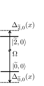
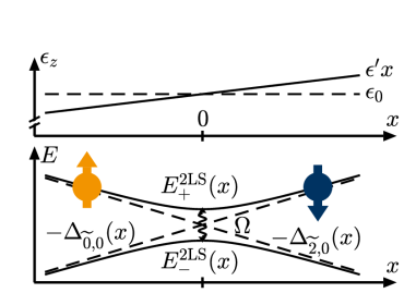
(a) (b) (c)

Figure 6: (a) The two rotational states $|\widetilde{0},0\rangle$ and $|\widetilde{2},0\rangle$ are coupled by a microwave with Rabi frequency $\Omega$. (b) The detunings $\Delta_{\widetilde{N},0}(x)$, where $N=0,2$ are position dependent due to a spatially non-uniform static electric field $\epsilon(x)=\epsilon_{0}+\epsilon^{\prime}x$. (c) Therefore, the micro wave coupling is resonant with the position-dependent Stark shifted energies (dashed lines) of two rotational states with opposite induced dipole moments (blue and orange arrows) at a particular value of the x coordinate which we choose as the origin of the coordinate system. This gives rise to the two dressed channels with energies $E_{\pm}^{\mathrm{2LS}}(x)$.

As already discussed in Sec. II.1 the BO approximation Burrows et al. (2017); Kazantsev et al. (1990); Dum and Olshanii (1996); Dutta et al. (1999); Ruseckas et al. (2005) assumes that the internal state of the molecules adiabatically follows the external motion, where the parametric dependence of the internal state on the position is given by Eq. (26). In particular, the Hamiltonian for the motion of a molecule prepared in the $+$ channel is given by

$$H_{\mathrm{2LS},++}^{\mathrm{ad}}=\frac{p_{x}^{2}}{2m}+E^{\mathrm{2LS}}_{+}(x)+V_{\mathrm{na}}(x),$$ (27)

where the nonadiabatic potential barrier is given by

$$V_{\mathrm{na}}(x)=\frac{\hbar^{2}}{2ms^{2}}\frac{1}{4}\frac{1}{[1+(x/s)^{2}]^{2}}.$$ (28)

A detailed derivation of the adiabatic Hamiltonian from Eq. (27) is provided in Appendix A.1. We focus on a parameter regime that is specified below, in which both the channel coupling and the nonadiabatic contribution to the effective BO potential from $A^{2}(x)$ are negligible. The validity of this approximation is discussed in detail in Appendix A.

The effective BO potential corresponding to the eigenvalue $E_{+}(x)$ forms a trap. This is because the induced dipole moments $\mathrm{d}^{\widetilde{2},0}_{z}$ and $\mathrm{d}^{\widetilde{0},0}_{z}$ have opposite sign as can be seen in Fig. 3(b), and thus the position-dependent Stark shifts $\Delta_{\widetilde{0},0}(x)$ for $x\gtrsim s$ and $\Delta_{\widetilde{2},0}(x)$ for $x\lesssim-s$ have opposite signs. For $\lvert x\rvert\ll s$ we approximate the BO trapping potential $E^{\mathrm{2LS}}_{+}(x)$ by a harmonic potential,

$$\begin{split}E^{\mathrm{2LS}}_{+}(x)&\approx\hbar\Omega/2\left[1-x_{0}^{2}/s^{2}+(x-x_{0})^{2}/s^{2}\right]\\ &=\Delta E+m\omega_{0}^{2}(x-x_{0})^{2}/2.\end{split}$$ (29)

The harmonic approximation is characterized by the effective trap frequency $\hbar\omega_{0}=\sqrt{\hbar\Omega\leavevmode\nobreak\ \hbar^{2}/(2ms^{2})}$, the position of the minimum $x_{0}/s=(1-\delta)/2\sqrt{\delta}$, and the energy shift $\Delta E=\hbar\Omega/2[1-(x_{0}/s)^{2}]$. In this harmonic potential, the size of the ground state is given by $l_{0}=\sqrt{\hbar/(m\omega_{0})}$, and for self-consistency we require $l_{0}/s\ll 1$. The effective potential $E_{-}(x)$ in the BO channel corresponding to the eigenstate $|-\rangle_{x}$ forms an inverted trap, and consequently this channel hosts a continuum of scattering states. The coupling between the BO channels leads to decay of the bound states in the $+$ channel to the continuum in the $-$ channel. The decay rate can be estimated by Fermi’s golden rule as

$$\frac{\Gamma_{\mathrm{2LS}}}{\omega_{0}}\approx 2\sqrt{\pi}\frac{l_{0}}{s}\exp\left[-8\left(\frac{s}{l_{0}}\right)^{2}\right].$$ (30)

A detailed derivation is provided in Appendix A. The adiabatic limit requires $\Gamma_{\mathrm{2LS}}/\omega_{0}\ll 1$ which is achieved for $l_{0}/s\ll 1$, in agreement with the harmonic approximation of $E_{+}(x)$. Because of the exponential factor in the rate Eq. (30) a moderately small ratio of $l_{0}/s=1/\sqrt{2}$ is sufficient to obtain a strongly suppressed decay rate of $\Gamma_{\mathrm{2LS}}/\omega_{0}<10^{-6}$. In the next section, we focus on the $+$ channel and discuss bound states of pairs of molecules due to spatially inhomogeneous dipole moments.

III.2 Dipolar interaction and interface bound state

Since the state $|+\rangle_{x}$ defined in Eq. (26) changes from $|+\rangle_{x}\to|\widetilde{0},0\rangle$ for $x\to+\infty$ to $|+\rangle_{x}\to|\widetilde{2},0\rangle$ for $x\to-\infty$, also the induced dipole moment $\mathrm{d}^{\mathrm{D}}_{z}(x)$ defined in Eq. (35) below varies in space and takes limiting values with opposite signs given by $\mathrm{d}^{\mathrm{D}}_{z}(x)\to\mathrm{d}_{z}^{\widetilde{0},0}$ and $\mathrm{d}^{\mathrm{D}}_{z}(x)\to\mathrm{d}_{z}^{\widetilde{2},0}$ for $x\to+\infty$ and $x\to-\infty$, respectively. Therefore, two molecules in the $+$ channel experience attractive induced dipolar interactions if they are located on opposite sides of the point $x_{0}$ where the dipole moment $\mathrm{d}_{z}(x)$ changes sign. If they are on the same side, they repel each other not (a). As we show in the following, this gives rise to the formation of bound states of two molecules close to $x_{0}$.

We consider now the full 3D geometry with a harmonic confinement $V_{\perp}(z)=m\omega_{\perp}^{2}z^{2}/2$ in the $z$ direction, whereas motion along the $y$ axis is unrestricted. The Hamiltonian for the motion of two molecules $j=1,2$ with position coordinates $\mathbf{r}_{j}=(x_{j},y_{j},z_{j})$ and momenta $\mathbf{p}_{j}$ is then given by

$$H_{2,\mathrm{2LS}}=\sum_{j=1,2}\left[\frac{\mathbf{p}_{j}^{2}}{2m}+H^{0}_{\mathrm{2LS}}(x_{j})+\frac{1}{2}m\omega_{\perp}^{2}z_{j}^{2}\right]$$ (31)

$$+U^{(1)}_{\mathrm{2LS}}(t)\otimes U^{(2)}_{\mathrm{2LS}}(t)\leavevmode\nobreak\ V_{\mathrm{dd}}(\mathbf{r}_{1}-\mathbf{r}_{2})\leavevmode\nobreak\ U_{\mathrm{2LS}}^{(2),\dagger}(t)\otimes{U^{(1),\dagger}_{\mathrm{2LS}}}(t),$$

where the dipolar interaction is given in Eq. (12) and the rotating-frame transformation $U^{(j)}_{\mathrm{2LS}}(t)=\exp\left[-i(E_{\widetilde{2},0}-E_{\widetilde{0},0})t/\hbar\,|\widetilde{0},0\rangle\langle\widetilde{0},0|\right]$ for the $j$^th particle. The wave function for two molecules in the $+$ BO channel can be written as

$$|\Psi\rangle=\int\mathrm{d}\mathbf{r}_{1}\mathrm{d}\mathbf{r}_{2}\,\Psi(\mathbf{r}_{1},\mathbf{r}_{2})|\mathbf{r}_{1},\mathbf{r}_{2}\rangle\otimes|+\rangle_{x_{1}}\otimes|+\rangle_{x_{2}}.$$ (32)

In the following, we neglect nonadiabatic corrections to the BO approximation. Upon projecting the Hamiltonian in Eq. (31) to the $+$ channel, the contribution $H_{\mathrm{2LS}}^{0}(x_{j})$ is replaced by the effective potential $E_{+}(x_{j})$. Further, the dipolar interaction for two molecules in the $+$ channel is given by

$$V_{\mathrm{dd}}^{+}(\mathbf{r}_{1},\mathbf{r}_{2})={}_{x_{1}}\langle+|\otimes{}_{x_{2}}\langle+|\left[U^{(1)}_{\mathrm{2LS}}(t)\otimes U^{(2)}_{\mathrm{2LS}}(t)\right.\\ \left.\times V_{\mathrm{dd}}(\mathbf{r}_{1}-\mathbf{r}_{2})\,U_{\mathrm{2LS}}^{{(2)},\dagger}(t)\otimes U_{\mathrm{2LS}}^{{(1)},\dagger}(t)\right]|+\rangle_{x_{1}}\otimes|+\rangle_{x_{2}}.$$ (33)

Due to the rotating-frame transformation $U_{\mathrm{2LS}}^{(j)}(t)$, certain contributions to the dipolar interaction acquire rapidly oscillating phase factors. These contributions average to zero, and we only keep the time-independent components. Then, the dipolar interaction can be written as

$$V_{\mathrm{dd}}^{+}(\mathbf{r}_{1},\mathbf{r}_{2})=\frac{\mathrm{d}^{\mathrm{D}}_{z}(x_{1})\mathrm{d}^{\mathrm{D}}_{z}(x_{2})+2\mathrm{d}^{\mathrm{E}}_{z}(x_{1})\mathrm{d}^{\mathrm{E}}_{z}(x_{2})}{|\mathbf{r}_{1}-\mathbf{r}_{2}|^{3}}\\ \times\left[1-3\frac{(z_{1}-z_{2})^{2}}{|\mathbf{r}_{1}-\mathbf{r}_{2}|^{2}}\right],$$ (34)

where the “direct” dipole moments are

$$\begin{split}\mathrm{d}^{\mathrm{D}}_{z}(x)&={}_{x}\langle+|\left(|\widetilde{2},0\rangle\langle\widetilde{2},0|\hat{\mathrm{d}}_{z}|\widetilde{2},0\rangle\langle\widetilde{2},0|\right.\\ &\left.\mathrel{\hphantom{=}}+|\widetilde{0},0\rangle\langle\widetilde{0},0|\hat{\mathrm{d}}_{z}|\widetilde{0},0\rangle\langle\widetilde{0},0|\right)|+\rangle_{x}\\ &=\mathrm{d}_{z}^{\widetilde{2},0}\left(\frac{1-\delta}{2}-\frac{1+\delta}{2}\frac{x}{\sqrt{s^{2}+x^{2}}}\right),\end{split}$$ (35)

and the “exchange” moments, which correspond to interaction processes that exchange the internal states of the molecules, read

$$\begin{split}\mathrm{d}^{\mathrm{E}}_{z}(x)&={}_{x}\langle+|{\widetilde{2},0}\rangle\langle\widetilde{2},0|\hat{\mathrm{d}}_{z}|\widetilde{0},0\rangle\langle{\widetilde{0},0}|+\rangle_{x}\\ &=\langle\widetilde{2},0|\hat{\mathrm{d}}_{z}|\widetilde{0},0\rangle\frac{1}{2}\frac{s}{\sqrt{s^{2}+x^{2}}}.\end{split}$$ (36)

In the following, we neglect contributions to $V_{\mathrm{dd}}^{+}(\mathbf{r}_{1},\mathbf{r}_{2})$ which involve $\mathrm{d}^{\mathrm{E}}_{z}(x)$. This is justified since $|\langle\widetilde{2},0|\hat{\mathrm{d}}_{z}|\widetilde{0},0\rangle|\ll|\mathrm{d}_{z}^{\widetilde{2},0}|,\leavevmode\nobreak\ |\mathrm{d}_{z}^{\widetilde{0},0}|$. We note that a corresponding relation does not apply, for example, for the pair of states $|\widetilde{0},0\rangle$ and $|\widetilde{1},0\rangle$. We further remark that the diagonal matrix elements of the dipole moment operator which enter Eq. (35) are not affected by the rotating-frame transformation which lead to the 2LS Hamiltonian (23). The position $x_{0}$ of the zero-crossing of $\mathrm{d}_{z}^{\mathrm{D}}(x)$ coincides with the minimum of $E_{+}(x)$ from Eq. (24) given above. For $l_{0}\ll s$ we expand

$$\mathrm{d}_{z}^{\mathrm{D}}(x_{0}+x)\approx-\mathrm{d}_{z}^{\widetilde{2},0}\frac{4\delta^{3/2}}{(1+\delta)^{2}}\frac{x}{s}$$ (37)

to linear order in $x/s$ around $x_{0}$. Here and in the following, the $x$-coordinates $x_{1,2}$ of the molecules are measured from the zero-crossing $x_{0}$ of the induced dipole moment (35). Then, the projection of the two-molecule Hamiltonian (31) to the $+$ channel reads

$$H_{2,\mathrm{2LS}}^{+}=\sum_{j=1,2}\left[\frac{\mathbf{p}_{j}^{2}}{2m}+E^{\mathrm{2LS}}_{+}(x_{j})+\frac{1}{2}m\omega_{\perp}^{2}z_{j}^{2}\right]+V_{\mathrm{dd}}^{+}(\mathbf{r}_{1},\mathbf{r}_{2}).$$ (38)

Since the induced dipole moment (35) is oriented along the $z$ axis, inelastic head-to-tail collisions of the two molecules can be suppressed through tight confinement in this direction. We assume that the trapping frequency $\omega_{\perp}$ is sufficiently large such that excited states in the potential $V_{\perp}(z)$ are energetically inaccessible, and the molecules reside in the ground state. Then, the wave function $\Psi(\mathbf{r}_{1},\mathbf{r}_{2})$ in Eq. (32) factorizes as $\Psi(\mathbf{r}_{1},\mathbf{r}_{2})=\Psi_{\parallel}(\boldsymbol{\rho}_{1},\boldsymbol{\rho}_{2})\,\phi^{0}_{\perp}(z_{1})\,\phi^{0}_{\perp}(z_{2})$ where $\boldsymbol{\rho}_{j}=\left(x_{j},y_{j}\right)$. The harmonic oscillator ground state wave function reads

$$\phi^{0}_{\perp}(z)=\frac{1}{\sqrt{l_{\perp}\sqrt{\pi}}}\exp\left(-\frac{z^{2}}{2l_{\perp}^{2}}\right),$$ (39)

where $l_{\perp}^{2}=\hbar/(m\omega_{\perp})$ is the corresponding oscillator length. Under these conditions, which also imply $l_{\perp}\ll l_{0}$, the motion of the molecules is confined to the $xy$ plane, and the system becomes effectively 2D. Up to the zero-point energy in the harmonic confinement in the $z$ direction, the Hamiltonian for the 2D motion of the two molecules is given by

$$H_{\mathrm{2D}}=\sum_{j=1,2}\left[\frac{\mathbf{p}_{j}^{2}}{2m}+E^{\mathrm{2LS}}_{+}(x_{j})\right]+V_{\mathrm{2D}}(\boldsymbol{\rho}_{1},\boldsymbol{\rho}_{2}).$$ (40)

We obtain the effective 2D dipolar interaction by integrating out the tightly confined $z$ direction, which yields

$$\begin{split}V_{\mathrm{2D}}(\boldsymbol{\rho}_{1},\boldsymbol{\rho}_{2})&=\int\mathrm{d}z_{1}\mathrm{d}z_{2}\,\lvert\phi^{0}_{\perp}(z_{1})\rvert^{2}\,\lvert\phi^{0}_{\perp}(z_{2})\rvert^{2}\,V_{\mathrm{dd}}^{+}(\mathbf{r}_{1},\mathbf{r}_{2})\\ &=\mathrm{d}_{z}^{\mathrm{D}}(x_{1})\mathrm{d}_{z}^{\mathrm{D}}(x_{2})v_{\mathrm{2D}}(\rho).\end{split}$$ (41)

That is, the effective 2D dipolar interaction can be written as the product of position-dependent dipole moments $\mathrm{d}_{z}^{\mathrm{D}}(x_{j})$ and an interaction potential $v_{\mathrm{2D}}(\rho)$ which depends only on the relative distance in the $xy$ plane, $\rho^{2}=(x_{1}-x_{2})^{2}+r_{y}^{2}$, where $r_{y}=y_{1}-y_{2}$ is the relative coordinate in the $y$ direction. The interaction potential is given by

$$v_{\mathrm{2D}}(\rho)=\frac{1}{\sqrt{8\pi}l_{\perp}^{3}}\exp\!\left(\frac{\rho^{2}}{4l_{\perp}^{2}}\right)\left[\left(2+\frac{\rho^{2}}{l_{\perp}^{2}}\right)K_{0}\!\left(\frac{\rho^{2}}{4l_{\perp}^{2}}\right)\right.\\ \left.-\frac{\rho^{2}}{l_{\perp}^{2}}K_{1}\!\left(\frac{\rho^{2}}{4l_{\perp}^{2}}\right)\right].$$ (42)

Here, $K_{n}(z)$ is the modified Bessel function of the second kind. At large distances $\rho\gg l_{\perp}$, the interaction potential assumes the characteristic dipolar form $v_{\mathrm{2D}}(\rho)\sim 1/\rho^{3}$; At short distances $\rho\ll l_{\perp}$ it diverges logarithmically, $v_{\mathrm{2D}}(\rho)\sim\sqrt{2/\pi}/l_{\perp}^{3}\ln(\rho/l_{\perp})$.

The setup we consider is translationally invariant along the $y$ axis and, therefore, the motion of two molecules in this direction factorizes into center-of-mass (COM) and relative components, $\Psi_{\parallel}(\boldsymbol{\rho}_{1},\boldsymbol{\rho}_{2})=\psi(x_{1},x_{2},r_{y})\,\xi(R_{y})$, where $R_{y}=(y_{1}+y_{2})/2$ is the COM coordinate. Possible bound states are negative-energy solutions of the two-body SE

$$\left[\sum_{j=1,2}\left(-\frac{\hbar^{2}}{2m}\frac{\partial^{2}}{\partial x_{j}^{2}}+\frac{1}{2}m\omega_{0}^{2}x_{j}^{2}\right)-\frac{\hbar^{2}}{m}\frac{\partial^{2}}{\partial r_{y}^{2}}\right.\\ \left.\vphantom{\sum_{j=1,2}\left(-\frac{\hbar^{2}}{2m}\frac{\partial^{2}}{\partial x_{j}^{2}}+\frac{1}{2}m\omega_{0}^{2}x_{j}^{2}\right)}+V_{\mathrm{2D}}(x_{1},x_{2},r_{y})\right]\psi(x_{1},x_{2},r_{y})\\ =\left(E_{B}+\hbar\omega_{0}\right)\psi(x_{1},x_{2},r_{y}),$$ (43)

where we replaced the effective potential $E_{+}(x)$ in the $+$ BO channel by its harmonic approximation (29), and we omitted the energy offset $\Delta E$. The binding energy $E_{B}$ is measured from the ground state energy of the noninteracting two particle problem, which is $2\times\hbar\omega_{0}/2$.

We solve this Eq. (43) numerically. Details are discussed in Appendix B, and we present our results in Fig. 7. As shown in Fig. 7(a), a bound state occurs for sufficiently strong induced dipolar interactions, where the strength of dipolar interactions is characterized by the ratio $a^{\widetilde{2},0}_{d}/l_{0}$ with

$$a^{\widetilde{2},0}_{d}=m\left[\frac{\mathrm{d}_{z}^{\widetilde{2},0}}{\hbar}\frac{4\delta^{3/2}}{(1+\delta)^{2}}\right]^{2}.$$ (44)

We note that while achievable binding energies are boosted if the characteristic length scale $l_{0}$ of this setup is on the order of tens of nanometers, the scheme suffers from a reduction of the dipolar moment in the vicinity of the interface. Figure 7(b) shows the wave function of the bound state for $l_{0}=1.5l_{\perp}$ and $a_{d}^{\widetilde{2},0}=69l_{0}$. Numerically, we find that the threshold value for the formation of a bound state depends only slightly on $l_{\perp}$. This is because $V_{\mathrm{2D}}(x_{1},x_{2},r_{y})$ is only modified in regions where $(x_{1}-x_{2})^{2}+r_{y}^{2}\lesssim l_{\perp}^{2}$, and in these regions, the probability amplitude $|\psi(x_{1},x_{2},r_{y})|^{2}$ is suppressed. The existence of a threshold value of the ratio $a^{\widetilde{2},0}_{d}/l_{0}$ implies that strong harmonic confinement suppresses the formation of the bound state.

These results can be understood qualitatively within a simplified model which we obtain from Eq. (43) by setting both the COM coordinate in the $x$ direction, $R_{x}=(x_{1}+x_{2})/2$, and the relative coordinate in the $y$ direction to zero, $R_{x}=r_{y}=0$. This yields an effective SE for the component of the wave function which describes the relative motion of the two molecules in the $x$ direction. The corresponding effective potential, which depends only on the relative coordinate $r_{x}=x_{1}-x_{2}$, contains contributions from the harmonic confinement and the dipolar interaction and is given by

$$V_{\mathrm{eff}}(r_{x})=\frac{1}{4}m\omega_{0}^{2}r_{x}^{2}+V_{\mathrm{2D}}(r_{x}/2,-r_{x}/2,0).$$ (45)

Figure 7 shows the effective potential for $a_{d}^{\widetilde{2},0}/l_{0}=0$ and $a_{d}^{\widetilde{2},0}/l_{0}=69$. In the former case, $V_{\mathrm{eff}}(r_{x})$ reduces to a harmonic potential. Then, the state with lowest energy is just the corresponding harmonic oscillator ground state. For $a_{d}^{\widetilde{2},0}/l_{0}=69$, the effective potential exhibits two minima at $r_{x}=\pm r_{x,0}\neq 0$. In this situation, it is energetically advantageous for the molecules to “pay the price” of climbing up to the first excited state in the harmonic potential and thus effectively increase their relative distance, since this allows them to reduce their total energy due to the contribution from the dipolar interaction in Eq. (45). Evidently, the formation of a bound state can be suppressed by increasing the strength of the harmonic confinement.

The above simplified model does not take symmetry requirements on the wavefunction for two identical fermions into account. To discuss this point, we return to the full SE (43). We note that a Hamiltonian which describes the motion of identical particles has to be symmetric under the exchange $\boldsymbol{\rho}_{1}\leftrightarrow\boldsymbol{\rho}_{2}$ of the coordinates of the particles. The Hamiltonian in Eq. (43) obeys an even stronger symmetry: It is symmetric under the exchange of both only the $x$ coordinates, $x_{1}\leftrightarrow x_{2}$, and only the $y$ coordinates, $y_{1}\leftrightarrow y_{2}$. Therefore, also its eigenfunctions have definite parity under these operations, i.e., $\psi(x_{1},x_{2},r_{y})=\pm\psi(x_{2},x_{1},r_{y})$ and $\psi(x_{1},x_{2},r_{y})=\pm\psi(x_{1},x_{2},-r_{y})$. Overall, the two-body wave function for identical fermions has to be antisymmetric, $\psi(x_{1},x_{2},r_{y})=-\psi(x_{2},x_{1},-r_{y})$. Numerically, we find that the bound state wave function is antisymmetric with respect to $x_{1}\leftrightarrow x_{2}$, and symmetric under $y_{1}\leftrightarrow y_{2}$ (or, equivalently, $r_{y}\to-r_{y}$). Finally, we note that fermionic statistics imply that the probability of a close encounter of the molecules is strongly suppressed, i.e., $\psi(x_{1},x_{2},r_{y})\to 0$ for $x_{1}\to x_{2}$ and $r_{y}\to 0$. In comparison to bosonic molecules, this enhances the stability of fermionic molecules against chemical reactions Micheli et al. (2010). Apart from reduced stability, bound states also occur for pairs of bosonic molecules in the 2LS configuration. However, for bosons we expect an increased threshold value of the dipolar length. This expectation is based on the simplified model described above and on symmetry arguments: The simplified model suggests that in order to form a bound state, the relative motion of two molecules in the $x$ direction has to populate excited harmonic oscillator states. For fermions, antisymmetry of the total wavefunction implies that excited states with odd harmonic oscillator quantum numbers are admissable, and the lowest lying state that is compatible with this requirement is the first excited state. However, this state is excluded for bosons by symmetry. The necessity to invest at least two harmonic oscillator excitation quanta results in a higher threshold to form a bound state.

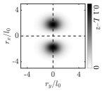
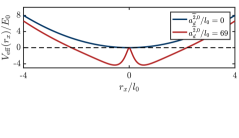
(a) (b) (c)

Figure 7: (a) Energy of the bound state in units of $E_{0}=\hbar^{2}/2ml_{0}^{2}$ as a function of the dipolar length $a^{\widetilde{2},0}_{d}$ defined in Eq. (44) for several values of $l_{0}/l_{\perp}$ and $s=\sqrt{2}l_{0}$. (b) Probability density $\int\mathrm{d}R_{x}|\psi(r_{x},R_{x},r_{y})|^{2}$ of the bound state, where $r_{x}=x_{1}-x_{2}$ and $R_{x}=(x_{1}+x_{2})/2$ are the relative and COM coordinates in the $x$ direction, for $l_{0}=1.5l_{\perp}$ and $a_{d}/l_{0}=69$. $L$ denotes the box size used in the numerical diagonalization of Eq. (43). (c) Effective potential (45) for the simplified model discussed in the main text.

III.3 Experimental parameters

	$\frac{m}{\mathrm{u}}$	$\frac{\mathcal{D}}{\mathrm{Debye}}$	$\frac{\hbar B}{h\mathrm{GHz}}$	$\frac{\epsilon_{0}}{\left(\mathrm{kV}/\mathrm{cm}\right)}$	$\frac{l_{0}}{\mathrm{nm}}$	$\frac{a^{\widetilde{2},0}_{d}}{l_{0}}$	$\frac{|E_{B}|}{h\mathrm{kHz}}$	$\frac{\Omega}{\mathrm{kHz}}$
KRbDe Marco et al. (2019)	$127$	$0.57$	$1.11$	$28.9$	61	$1.2$	0	$86$
Toy	$100$	$1.00$	$1$	$14.9$	54	$3.1$	0	$135$
NaKPark et al. (2015); Voges et al. (2019)	$63$	$2.72$	$2.83$	$15.5$	46	$17$	0	$307$
LiRb	$91$	$3.99$	$7.61$	$28.4$	36	$69$	66	$351$
LiCs	$139$	$5.39$	$6.54$	$18.1$	28	$241$	$564^{*}$	$374$

Table 2: A list of relevant parameters for different fermionic polar molecules Żuchowski et al. (2013); Aymar and Dulieu (2005). For all molecular species, the offset field is chosen as $\epsilon_{0}=7.5\,\hbar B/\mathcal{D}$ and the gradient field is fixed to $\epsilon^{\prime}=3.5\,(\mathrm{kV}/\mathrm{cm})/\mathrm{mm}$ and $l_{0}=1.5\,l_{\perp}$ holds. The asterisk ^∗ marks binding energies which exceed the single-particle level spacing in the potential well along the confined $z$-axis, $\lvert E_{B}\rvert>\hbar^{2}/(2ml_{\perp}^{2})$, and thus go beyond the range of validity of our analysis which assumes that the molecules populate only the lowest-energy single-particle state.

In this section, we discuss the optimal choice of experimental parameters for the realization of an interface bound state. From a single-particle point of view we require the decay rate of molecules in the $+$ channel given in Eq. (30) to be small, $\Gamma_{\mathrm{2LS}}/\omega_{0}\ll 1$, which is guaranteed for $l_{0}/s\ll 1$. However, even a moderately small ratio of $l_{0}/s=1/\sqrt{2}$ leads to $\Gamma_{\mathrm{2LS}}/\omega_{0}<10^{-6}$, such that the lifetime of molecules in the $+$ channel is well above any experimentally relevant time scale. The relation $l_{0}/s=1/\sqrt{2}$ can be rearranged as

$$\hbar\Omega=2\left[\epsilon^{\prime}\mathrm{d}_{z}^{\widetilde{2},0}(1+\delta)\frac{\hbar}{\sqrt{m}}\right]^{2/3},$$ (46)

such that $\Omega$ is fixed for a given value of $\epsilon^{\prime}$. This can be used to determine the harmonic oscillator length in the adiabatic regime as

$$l_{0}=\sqrt{2}\left(\frac{\hbar^{2}}{2m}\frac{1}{\epsilon^{\prime}\mathrm{d}_{z}^{\widetilde{2},0}\frac{1+\delta}{2}}\right)^{1/3}.$$ (47)

As $l_{0}$ sets the length and energy scale of the problem, the denominator in the above expression should be as large as possible. In current experiments, the electric field gradient is limited by the apparatus. Therefore, the difference between induced dipole moments $|\mathrm{d}_{z}^{\widetilde{2},0}(1+\delta)|=|\mathrm{d}_{z}^{\widetilde{2},0}-\mathrm{d}_{z}^{\widetilde{0},0}|$ has to be maximized. This boils down to finding the optimal value of the electric offset field, which is $\epsilon_{0}=7.5\,\hbar B/\mathcal{D}$. In turn, this implies $\mathrm{d}_{z}^{\widetilde{0},0}=0.74\,\mathcal{D}$, $\mathrm{d}_{z}^{\widetilde{2},0}=-0.26\,\mathcal{D}$ and $\delta=2.81$. As an example, we consider the LiRb molecule with parameters $m=91\,\mathrm{u}$, $\mathcal{D}=3.99\,\mathrm{Debye}$. Further, we take the electric field gradient to be $\epsilon^{\prime}=3.5\,\mathrm{(kV/cm)/mm}$. Then, with the optimal value $\epsilon_{0}=7.5\,\hbar B/\mathcal{D}$ of the offset field, the harmonic oscillator length evaluates to $l_{0}=36\,\mathrm{nm}$, which is considerably below optical length scales. For the same parameters, the dipolar length is given by $a_{d}^{\widetilde{2},0}/l_{0}=69$, which is above the threshold value for the appearance of a bound state. As can be seen in Fig. 7(a), the corresponding binding energy is $|E_{B}|=2\pi\times 66\,\mathrm{kHz}\,\hbar$ for the given parameters. In comparison, recent experiments with KRb De Marco et al. (2019) reached temperatures which correspond to a much lower energy of $50\,\mathrm{nK}\,k_{\mathrm{B}}=2\pi\times 1\,\mathrm{kHz}\,\hbar$. We list additional parameters for different species of polar molecules in Table 2.

We finally point out that the dipolar length scales as $a_{d}^{\widetilde{2},0}/l_{0}\propto\mathcal{D}^{2}\left(\mathcal{D}\epsilon^{\prime}\right)^{1/3}m^{4/3}$ with a prefactor that depends on the value of the offset field $\epsilon_{0}$. In experiments, this dependence on $\epsilon_{0}$ can be used to tune the dipolar length by adjusting the value of $\epsilon_{0}$, and thus cross the threshold for the formation of a bound state.

III.4 Adiabatic loading

To conclude this section, we present an experimental protocol to adiabatically prepare molecules in the $+$ channel. The electric offset field is kept at a constant value $\epsilon_{0}$ throughout the protocol, while the gradient field $\epsilon^{\prime}$ as well as the Rabi coupling $\Omega$ in the 2LS Hamiltonian (23) are set to zero initially. Further, we assume that the molecules are prepared in the rotational state $|\widetilde{0},0\rangle$, and that they are trapped in an auxiliary optical potential $V_{\mathrm{aux}}(x)$, which is switched off at the end of the protocol.

The first step is to turn on the Rabi coupling in the 2LS Hamiltonian (23), where the detunings are chosen such that $\Delta_{\widetilde{2},\widetilde{0}}=\Delta_{\widetilde{2},0}-\Delta_{\widetilde{0},0}<0$ and $\lvert\Delta_{\widetilde{2},\widetilde{0}}\rvert/\Omega\gg 1$, implying $|+\rangle\approx|\widetilde{0},0\rangle$. Next, the magnitue of the detunings is adiabatically reduced ($\lvert\partial_{t}{\Delta}_{\widetilde{2},\widetilde{0}}\rvert/\Omega^{2}\ll 1$) to zero. Under this condition, the molecules remain in the instantaneous excited eigenstate $|+\rangle$ and at the end of the adiabatic sweep this state is given by $|+\rangle=(|\widetilde{0},0\rangle+|\widetilde{2},0\rangle)/\sqrt{2}$. The final state to prepare molecules in $|+\rangle_{x}$ from Eq. (26) is to adiabatically turn off the auxiliary optical potential while ramping up the electric gradient field $\epsilon^{\prime}$, such that the effective harmonic confinement in the $+$ channel ($E_{+}^{\mathrm{2LS}}(x)+V_{\mathrm{aux}}(x)$) stays approximately constant. At the same time, states in the $-$ channel evolve from being trapped to being antitrapped. Due to nonadiabatic channel couplings, there are narrow avoided crossings between excited motional states in the $-$ channel and states in the $+$ channel. This avoided crossings are exponentially small, see Appendix A.3.3, and have to be passed nonadiabatically.

IV Conclusion and Outlook

To summarize, we presented two approaches for engineering quantum many-body systems with polar molecules by employing the coupling of rotational states via external laser or MW fields and electric field gradients. The first approach builds on a Raman coupled $\Lambda$-systems, where the strong electric field gradient of a standing laser field leads to the generation of a single particle potential barrier on the nanoscale. The second scheme generates spatially modulated electric dipoles and thus dipolar interactions by MW mixing in the presence of electric DC field gradients.

Nanostructured optical barriers in combination with optical lattice potentials enable the generation of bilayer systems, where the layers are separated by only few tens of nanometers. The resulting many-body systems are described by a Hamiltonian of the form

$$H=H_{L}+H_{R}+\sum_{{i_{L}},{j_{R}}}V_{LR}(\boldsymbol{\rho}_{i_{L}}-\boldsymbol{\rho}_{j_{R}}),$$ (48)

where $H_{\alpha}=\sum_{i}(-\hbar^{2}/2m)\nabla^{2}_{i_{\alpha}}+\sum_{i<j}V_{\alpha\alpha}(\boldsymbol{\rho}_{i_{\alpha}}-\boldsymbol{\rho}_{j_{\alpha}})$ is the Hamiltonian which describes the motion and interactions of molecules within the layer $\alpha=L,R$, $\boldsymbol{\rho}_{i_{\alpha}}$ the position of molecule $i$ in the layer $\alpha=L,R$, and $V_{LR}$ describes the interaction between molecules in different layers. The strong enhancement of $V_{LR}$ due to the small layer separation makes interesting few- and many-body physics experimentally accessible for molecules with a dipole moment of less than one Debye. Examples include the formation of interlayer bound states as discussed in this work, the BCS to BEC crossover for fermionic molecules Zinner et al. (2012), bilayer quantum Hall physics and—if the motion of molecules within each layers is restricted further to a one-dimensional channel—ladder physics (see, for example, Ref. Baranov et al. (2012) and references therein). We note that this scheme can be applied to atoms carrying magnetic dipole moments as originally proposed in Ref. Ła̧cki et al. (2016).

The second, all electric approach enables the realization of many-body systems in which the induced dipole moment $\mathrm{d}_{z}^{+}(z)$ changes sign on a spatial scale of tens of nanometers. The corresponding many-body Hamiltonian is given by

$$H=\sum_{i}\left[-\frac{\hbar^{2}}{2m}\nabla^{2}_{i}+E_{+}^{\mathrm{2LS}}(x_{i})\right]+\sum_{i<j}\frac{\mathrm{d}^{+}_{z}(x_{i})\mathrm{d}^{+}_{z}(x_{j})}{|\boldsymbol{\rho}_{i}-\boldsymbol{\rho}_{j}|^{3}},$$ (49)

where $E_{+}^{\mathrm{2LS}}(x)$ is an effective single-particle potential, whose explicit form is stated in Eq. (24). At $x=0$, the induced dipole moment vanishes. Two molecules which are located on opposite sides of this interface at $x=0$ interact attractively and can form bound states, while molecules on the same side of the interface always repel each other. The observation of these bound states under current experimental conditions is possible for molecules with dipole moments of a few Debye. In a system of fermionic molecules, the formation of interface bound state can cause a transition from fermionic to bosonic behavior, and it is an interesting question for further studies which quantum phases can be realized in such systems. We finally note that this all electric scheme can be applied with molecules for which the complexity of the level structure makes the optical manipulation with laser light challenging. Moreover, this technique can also be adapted to atoms or molecules with magnetic dipole moments by coupling to an external magnetic field gradient Hofferberth et al. (2006); Perrin and Garraway (2017), which requires gradients on the order of thousands of G/mm not (b).

In summary, the promise of enhanced energy scales and novel interaction terms modulated on spatial scales of tens of nanometers provides an interesting new avenue for many-body physics, including BCS–BEC or fractional quantum Hall phases.

Acknowledgments –The authors thank M. Lacki, D. Petter and M. Mark for discussions. P.Z. thanks JILA for hospitality as Visiting Fellow in September 2018, where part of this work was done. Work at Innsbruck is supported by the European Union program Horizon 2020 under Grants Agreement No. 817482 (PASQuanS) and No. 731473 (QuantERA via QTFLAG), the US Air Force Office of Scientific Research (AFOSR) via IOE Grant No. FA9550-19-1-7044 LASCEM, by the Simons Collaboration on Ultra-Quantum Matter, which is a grant from the Simons Foundation (651440, P.Z.), by a joint-project grant from the FWF (I 4426, RSF/Russia 2019), and by the Institut für Quanteninformation. Work at Boulder is supported by the Army Research Office (ARO) Grant W911NF-19-1-0210, the National Science Foundation (NSF) Grant No. PHY-1820885, JILA-NSF Grant No. PFC-1734006, and the National Institute of Standards and Technology (NIST).

Appendix A Validity of the Born-Oppenheimer approximation

Due to the large separation of typical energy scales between the internal rotational and the external motional degrees of freedom of polar molecules, the internal state of a molecule follows its motion essentially adiabatically, as discussed in the main text Secs. II and III. In particular, the internal state changes according to the spatial variation of applied electric fields. Deviations from such fully adiabatic dynamics are discussed in this Appendix. First, we discuss the transformation of the Hamiltonian into the BO basis and classify diagonal and off-diagonal corrections. Then, we study the impact of diagonal nonadiabatic corrections on wave functions in the BO channels of interest, which is the zero-energy channel in the $\Lambda$-system and the $+$ channel in the 2LS. Last, we quantify the decay of states in these BO channels due to nonadiabatic channel couplings. We estimate the corresponding decay rates, which are given in Eqs. (9) and (30) in the main text, using Fermi’s golden rule, and show that they are exponentially suppressed.

A.1 Basis transformation

For the sake of completeness we summarize how to perform the BO approximation Burrows et al. (2017); Kazantsev et al. (1990); Dum and Olshanii (1996); Dutta et al. (1999); Ruseckas et al. (2005) for the $\Lambda$-system Ła̧cki et al. (2016); Jendrzejewski et al. (2016) discussed in Sec. II.1 and apply these ideas to the TLS from Sec. III.1. As a first step the system Hamiltonian has to be transformed into the spatially dependent BO basis. In particular, we consider the Hamiltonians in Eqs. (2) and (22), which describe the dynamics of a single molecule in the $\Lambda$-system and 2LS setups, respectively. By introducing an index $\alpha\in\{\Lambda,\,\mathrm{2LS}\}$, these Hamiltonians can be brought to the common form

$$H_{\alpha}=\frac{p_{z}^{2}}{2m}+\delta_{\Lambda,\alpha}\,V_{L}(z)+H^{0}_{\alpha}(z).$$ (50)

The Kronecker delta $\delta_{\Lambda,\alpha}$ ensures that the external confinement $V_{L}(z)$ is only present in the $\Lambda$-system. We further note that in the 2LS, the $z$ coordinate has to be replaced by $x$. The adiabatic or BO basis is formed by the eigenvectors of $H^{0}_{\alpha}(z)$, which satisfy $H^{0}_{\alpha}(z)\,|\sigma_{\alpha}\rangle_{z},=E^{\alpha}_{\sigma}(z)|\sigma_{\alpha}\rangle_{z}$, and depend on the position $z$. For the $\Lambda$-system, where $\sigma=0,\pm$, the eigenvectors and energies are given in Eqs. (4) and (5); for the 2LS, $\sigma=\pm$, and the eigenvectors and energies are given in Eqs. (24) and (26). To transform the Hamiltonian (50) to the BO basis, we expand the state of a molecule as $|\Psi\rangle=\int\mathrm{d}z\sum_{\sigma}\Psi_{\sigma}(z)|z\rangle\otimes|\sigma_{\alpha}\rangle_{z}$, where $|z\rangle$ is an eigenstate of the position operator. The effective Hamiltonian $H_{\alpha}^{\mathrm{ad}}$ for the wave functions $\Psi_{\sigma}(z)$ in the adiabatic basis can be obtained from Eq. (50) by shifting the momentum operator according to $p_{z}\rightarrow p_{z}-A_{\alpha}(z)$, where $A_{\alpha}(z)_{\sigma,\sigma^{\prime}}=-{}_{z}\langle\sigma_{\alpha}|p_{z}|\sigma^{\prime}_{\alpha}\rangle_{z}$ can be interpreted as a gauge potential,

$$H_{\alpha}^{\mathrm{ad}}=\frac{p_{z}^{2}-\{p_{z},A_{\alpha}(z)\}+A_{\alpha}^{2}(z)}{2m}+D_{\alpha}(z),$$ (51)

with BO potentials

$$\begin{split}D_{\Lambda}(z)&=V_{L}(z)+\mathrm{diag}\left[E^{\Lambda}_{+}(z),\,0,\,E^{\Lambda}_{-}(z)\right],\\ D_{\mathrm{2LS}}(z)&=\mathrm{diag}\left[E^{\mathrm{2LS}}_{+}(z),\,E^{\mathrm{2LS}}_{-}(z)\right].\end{split}$$

The gauge potential for the $\Lambda$-system can be found in the supplementary material of Ła̧cki et al. (2016) or in the main text of Ref.Jendrzejewski et al. (2016) and is given by

$$A_{\Lambda}(z)=\frac{i\hbar}{l\sqrt{2}}\frac{1}{1+(z/l)^{2}}\begin{pmatrix}0&1&0\\ -1&0&1\\ 0&-1&0\end{pmatrix}$$ (52)

for $\Delta=0$ and $l\ll\lambda_{c}$. For the 2LS, the gauge potential reads

$$A_{\mathrm{2LS}}(z)=\frac{i\hbar}{2s}\frac{1}{1+(z/s)^{2}}\begin{pmatrix}0&-1\\ 1&0\end{pmatrix}.$$ (53)

The contributions from $A_{\alpha}(z)$ are twofold: Since $A_{\alpha}(z)$ is purely off-diagonal in the adiabatic basis spanned by the states $|\sigma_{\alpha}\rangle_{z}$, the term $\{p_{z},A_{\alpha}(z)\}$ describes nonadiabatic channel couplings; On the other hand, $A_{\alpha}(z)^{2}$ contains for the $\Lambda$-system both off-diagonal channel couplings and diagonal contributions, and for the 2LS only diagonal contributions. Diagonal contributions give rise to repulsive potential barriers. If nonadiabatic channel couplings are negligible, the Hamiltonian for a BO channel $\sigma$ is given by

$$H_{\alpha,\sigma\sigma}^{\mathrm{ad}}=\frac{p^{2}_{z}}{2m}+D_{\alpha}(z)_{\sigma\sigma}+V_{\mathrm{na}}(z),$$ (54)

where $V_{\mathrm{na}}(z)={(A_{\alpha})^{2}{}_{\sigma\sigma}}/{2m}$ is the nonadiabatic potential barrier. For $\sigma=0$ and $\sigma=+$ we obtain the Hamiltonians in Eqs. (7) and (27) for the $\Lambda$-system and 2LS, respectively. In the following sections, we specify the conditions under which nonadiabatic channel couplings are negligible.

A.2 Harmonic confinement in the presence of the barrier

The dynamics of molecules in the zero-energy channel in the $\Lambda$-system and in the $+$ channel in the 2LS is described by the Hamiltonians in Eqs. (7) and (27), respectively. Both Hamiltonians take the same form if we treat for the 2LS the effective BO potential $E_{+}(x)$ in the $+$ channel in the harmonic approximation (29) and neglect the energy shift $\Delta E$. Then, the generic Hamiltonian in the BO channel of interest reads

$$H=-\frac{\hbar^{2}}{2m}\frac{d^{2}}{dz^{2}}+\frac{1}{2}m\omega_{L}^{2}z^{2}+\frac{\hbar^{2}}{2ml^{2}}\frac{1-\lambda^{2}}{(1+z^{2}/l^{2})^{2}},$$ (55)

where the last term corresponds to the diagonal nonadiabatic correction. The parameter $\lambda$ takes the value $\lambda=0$ for the $\Lambda$-system. Instead, for the 2LS, $\lambda=\sqrt{3}/2$, and one should replace the $z$ coordinate by $x$, $\omega_{L}$ by $\omega_{0}$, and $l$ by $s$.

In the 2LS, we are interested in the limit $l_{0}/s\ll 1$, where $l_{0}=\sqrt{\hbar/(m\omega_{0})}$ is the characteristic length scale associated with the frequency $\omega_{0}$. This inequality implies that the spacing of energy levels in the harmonic potential in Eq. (55) is much larger than the strength of the nonadiabatic potential, $\hbar\omega_{0}\gg\hbar^{2}/(2ms^{2})$. Under this condition, the nonadiabatic potential is indeed only a negligibly small perturbation.

In contrast, in the $\Lambda$-system, we require the inverted relation $a_{L}\gg l$, where $a_{L}$ is the length scale associated with $\omega_{L}$. This condition guarantees that the nonadiabatic potential barrier is much narrower than a single well in an optical lattice potential as illustrated in Fig. 4(a). As we show in the following, this condition also implies that low-energy eigenstates of the Hamiltonian (55) are strongly suppressed inside the barrier. We thus consider the eigenvalue equation of the Hamiltonian (55),

$$H\psi_{\lambda}(z)=E\psi_{\lambda}(z).$$ (56)

It is convenient to introduce the new independent variable $\overline{z}=z/l$ and rewrite this equation as

$$\left[-\frac{d^{2}}{d\overline{z}^{2}}+\frac{l^{4}}{a_{L}^{4}}\overline{z}^{2}+\frac{1-\lambda^{2}}{(1+\overline{z}^{2})^{2}}\right]\psi_{\lambda}(\overline{z})=\frac{2ml^{2}}{\hbar^{2}}E\psi_{\lambda}(\overline{z}).$$ (57)

For energies smaller than the height of the barrier, $E\ll\hbar^{2}/(2ml^{2})$, and inside the barrier, $\left|\overline{z}\right|\lesssim 1$, one can neglect both the harmonic potential and the right-hand side of this equation, such that the behavior of low-energy wave functions becomes energy independent. To establish this universal behavior, we consider the zero-energy solution $\varphi_{\lambda}(\overline{z})$ of the SE (57),

$$\left[\frac{d^{2}}{d\overline{z}^{2}}-\frac{1-\lambda^{2}}{(1+\overline{z}^{2})^{2}}\right]\varphi_{\lambda}(\overline{z})=0.$$ (58)

We can find a general solution of this equation by introducing the new independent variable $y=\arctan(\overline{z})$, such that the equation takes the form

$$\left[\frac{d^{2}}{dy^{2}}-2\tan(y)\frac{d}{dy}-\left(1-\lambda^{2}\right)\right]\varphi_{\lambda}(\overline{z})=0.$$ (59)

After introducing the new unknown function $g_{\lambda}(y)=\varphi_{\lambda}(y)/\cos(y)$, we finally obtain

$$\left(\frac{d^{2}}{dy^{2}}-\lambda^{2}\right)g_{\lambda}(y)=0.$$ (60)

This equation can easily be solved and the general solution of Eq. (58) then reads

$$\varphi_{\lambda}(\overline{z})=\sqrt{1+\overline{z}^{2}}\left\{A\cos[\lambda\arctan(\overline{z})]\vphantom{\frac{B}{\lambda}}\right.\\ \left.+\frac{B}{\lambda}\sin[\lambda\arctan(\overline{z})]\right\},$$ (61)

where $A$ and $B$ are unknown constants. The general solution $\varphi_{\lambda}(\overline{z})$ can be used to formulate the effective “boundary conditions” which connect the wave function and its derivative on different sites of the barrier. These conditions are applicable for wave functions which change on a scale that is much larger than the width of the barrier. In other words, the corresponding eigenenergies are much smaller than the height of the barrier. The “boundary conditions” are given by

$$\begin{split}\psi_{\lambda}^{\prime}(0^{+})+\psi_{\lambda}^{\prime}(0^{-})&=s\lambda\tan\left(\frac{\pi\lambda}{2}\right)\left[\psi^{\prime}_{\lambda}(0^{+})-\psi^{\prime}_{\lambda}(0^{-})\right],\\ \psi_{\lambda}(0^{+})-\psi_{\lambda}(0^{-})&=-s\lambda\cot\!\left(\frac{\pi\lambda}{2}\right)\left[\psi_{\lambda}^{\prime}(0^{+})+\psi_{\lambda}^{\prime}(0^{-})\right],\end{split}$$ (62)

where $\psi_{\lambda}(0^{\pm})$ and $\psi^{\prime}_{\lambda}(0^{\pm})$ are the values of the wave function and its derivative, respectively, on the right and left side of the barrier.

To derive the above conditions, let us consider the asymptotics of $\varphi_{\lambda}(\overline{z})$ for $\overline{z}\gg 1$,

$$\varphi_{\lambda}(\overline{z})\approx\left[A\lambda\sin\!\left(\frac{\pi\lambda}{2}\right)-B\cos\!\left(\frac{\pi\lambda}{2}\right)\right]\\ +\left[A\cos\!\left(\frac{\pi\lambda}{2}\right)+\frac{B}{\lambda}\sin\!\left(\frac{\pi\lambda}{2}\right)\right]\overline{z},$$ (63)

and for $\overline{z}\ll-1$

$$\varphi_{\lambda}(\overline{z})\approx\left[A\lambda\sin\!\left(\frac{\pi\lambda}{2}\right)+B\cos\!\left(\frac{\pi\lambda}{2}\right)\right]\\ +\left[-A\cos\!\left(\frac{\pi\lambda}{2}\right)+\frac{B}{\lambda}\sin\!\left(\frac{\pi\lambda}{2}\right)\right]\overline{z}.$$ (64)

These asymptotics have to be matched with the wave function and its derivatives for $\overline{z}\sim\pm 1$, $\psi(\overline{z})\approx\psi_{\lambda}(0^{\pm})+\psi^{\prime}_{\lambda}(0^{\pm})\overline{z}$. This gives

$$\begin{split}\psi_{\lambda}(0^{\pm})&=A\lambda\sin\!\left(\frac{\pi\lambda}{2}\right)\mp B\cos\!\left(\frac{\pi\lambda}{2}\right),\\ \psi^{\prime}_{\lambda}(0^{\pm})&=\pm A\cos\!\left(\frac{\pi\lambda}{2}\right)+\frac{B}{\lambda}\sin\!\left(\frac{\pi\lambda}{2}\right).\end{split}$$ (65)

After excluding the unknown constants $A$ and $B$, and restoring the original units, we arrive at the conditions presented in Eq. (62).

The boundary conditions in Eq. (62) allow us to estimate the suppression of the wave function in the barrier region. For this purpose we restore the harmonic potential in Eq. (55) characterized by the frequency $\omega_{L}$ and the harmonic length $a_{L}$, which we assume to be much larger than the width of the barrier $l$, $a_{L}\gg l$. The eigenenergies and eigenfunctions of this problem can be obtained by matching the solution

$$y_{+}(\widetilde{z})=C_{+}\exp(-\widetilde{z}^{2}/2)\left[\frac{1}{\Gamma(\frac{1-\nu}{2})}\Phi\!\left(-\frac{\nu}{2};\frac{1}{2};\widetilde{z}^{2}\right)\right.\\ \left.-\frac{2\widetilde{z}}{\Gamma(-\frac{\nu}{2})}\Phi\!\left(\frac{1-\nu}{2};\frac{3}{2};\widetilde{z}^{2}\right)\right]$$ (66)

which decays exponentially for $\widetilde{z}\to+\infty$ where $\widetilde{z}=z/a_{L}$, with the solution

$$y_{-}(\widetilde{z})=C_{-}\exp(-\widetilde{z}^{2}/2)\left[\frac{1}{\Gamma(\frac{1-\nu}{2})}\Phi\!\left(-\frac{\nu}{2};\frac{1}{2};\widetilde{z}^{2}\right)\right.\\ \left.+\frac{2\widetilde{z}}{\Gamma(-\frac{\nu}{2})}\Phi\!\left(\frac{1-\nu}{2};\frac{3}{2};\widetilde{z}^{2}\right)\right]$$ (67)

which decays exponentially for $\widetilde{z}\to-\infty$, in the region of the barrier. Here, $\Gamma(\widetilde{z})$ is the Gamma function, $\Phi(a;b;\widetilde{z})$ the degenerate hypergeometric function, and $\nu=2E/\hbar\omega_{L}$ the energy measured in units of the harmonic oscillator spacing. For low-energy eigenstates, $E\ll\hbar^{2}/(2ml^{2})$, we can use the boundary conditions (62), which give the following equations:

$$\left[\frac{1}{\Gamma(\frac{1-\nu}{2})}+\frac{l}{a_{L}}\frac{2}{\Gamma(-\frac{\nu}{2})}\lambda\tan\!\left(\frac{\pi\lambda}{2}\right)\right](C_{+}+C_{-}) =0,$$ (68)

$$\left[\frac{1}{\Gamma(\frac{1-\nu}{2})}\frac{1}{\lambda}\tan\!\left(\frac{\pi\lambda}{2}\right)-\frac{l}{a_{L}}\frac{2}{\Gamma(-\frac{\nu}{2})}\right](C_{+}-C_{-}) =0.$$ (69)

These equations determine the eigenergies $\nu$. The eigenenergies of states which are symmetric with respect to $\widetilde{z}\to-\widetilde{z}$ fulfill

$$\frac{1}{\Gamma(\frac{1-\nu}{2})}+\frac{l}{a_{L}}\frac{2}{\Gamma(-\frac{\nu}{2})}\lambda\tan\!\left(\frac{\pi\lambda}{2}\right)=0,$$ (70)

where $C_{+}=C_{-}$ follows from Eq. (68). The corresponding eigenfunctions for $\left|z\right|\gtrsim l$ have the form

$$y_{\mathrm{sym}}(z)\sim\exp(-z^{2}/2a_{L}^{2})\left[\frac{l}{a_{L}}\lambda\tan\!\left(\frac{\pi\lambda}{2}\right)\right.\\ \left.\times\Phi\!\left(-\frac{\nu}{2};\frac{1}{2};\frac{z^{2}}{a_{L}^{2}}\right)+\frac{\left|z\right|}{a_{L}}\Phi\!\left(\frac{1-\nu}{2};\frac{3}{2};\frac{z^{2}}{a_{L}^{2}}\right)\right].$$ (71)

The eigenenergies of antisymmetric solutions, for which $C_{+}=-C_{-}$ results from Eq. (69), satisfy the equation

$$\frac{1}{\Gamma(\frac{1-\nu}{2})}\frac{1}{\lambda}\tan\!\left(\frac{\pi\lambda}{2}\right)-\frac{l}{a_{L}}\frac{2}{\Gamma(-\frac{\nu}{2})}=0,$$ (72)

and the wave functions for $\left|z\right|\gtrsim l$ are

$$y_{\mathrm{asym}}(z)\sim\exp(-z^{2}/2a_{L}^{2})\left[\mathrm{sign}(z)\frac{l}{a_{L}}\frac{\lambda}{\tan\!\left(\frac{\pi\lambda}{2}\right)}\right.\\ \left.\times\Phi\!\left(-\frac{\nu}{2};\frac{1}{2};\frac{z^{2}}{a_{L}^{2}}\right)+\frac{z}{a_{L}}\Phi\!\left(\frac{1-\nu}{2};\frac{3}{2};\frac{z^{2}}{a_{L}^{2}}\right)\right].$$ (73)

From Eqs. (71) and (73), we see that as stated above the wave function in the region of the barrier, $\left|z\right|\lesssim l$, is reduced by a factor $l/a_{L}\ll 1$, as compared to its typical values outside the barrier for $\left|z\right|\gtrsim l$.

A.3 Nonadiabatic channel couplings

We now turn to nonadiabatic channel couplings, which correspond to the terms $C_{\mathrm{na}}=\left[-\{p_{z},A(z)\}+A^{2}(z)\right]/(2m)$ and $-\{p_{x},A(x)\}/(2m)$ in Eq. (51) for the $\Lambda$-system and 2LS, respectively. In the $\Lambda$-system, we are interested in the zero-energy BO channel. The external potential confines the zero energy BO channel, whereas the effective potential in the $-$ channel does not confine states with energy bigger than $0$. Therefore, the $-$ channel hosts a continuum of scattering states, and the nonadiabatic channel coupling $\left[-\{p_{z},A(z)\}+A^{2}(z)\right]/(2m)$ induces decay of states in the zero-energy BO channel into the continuum in the $-$ channel. Below, we estimate the corresponding decay rate using Fermi’s golden rule. In the 2LS, we are interested in the $+$ channel, for which the effective potential is given by the BO potential in Eq. (27). Decay occurs again to the open $-$ channel.

A.3.1 DOS in the open channel

According to Fermi’s golden rule, the rate of decay of a given initial state to an open channel hosting a continuum of final states is determined by the product of the transition matrix element between the initial and final states, and the DOS in the open channel. In this section, we derive the DOS in the open channel, which corresponds to the $-$ BO channel in both the $\Lambda$-system and the 2LS. We neglect nonadibatic corrections to the effective potential in the $-$ channel. Moreover, for the $\Lambda$-sytem we are only interested in a spatial region of extension $|z-z_{0}|\lesssim a_{L}\ll 2\pi/k_{c}$, thus we expand $\sin(k_{c}z)\approx k_{c}z$, and for simplicity we consider for the 2LS the symmetric case $\delta=1$. Then, for both systems, the effective BO potential in the $-$ channel can be written as $-U(z)=-\hbar\sqrt{(\Omega/2)^{2}+(\Delta^{\prime}z)^{2}}$, where we use the following identification table:

	$\Omega$	$\Delta^{\prime}$
2LS	$\leavevmode\nobreak\ \Omega\leavevmode\nobreak\$	$\leavevmode\nobreak\ \Delta^{\prime}_{\widetilde{2},0}\leavevmode\nobreak\$
$\Lambda$-system	$\leavevmode\nobreak\ \Omega_{p}\leavevmode\nobreak\$	$\leavevmode\nobreak\ \Omega_{c}k_{c}/2$

For the 2LS the $z$ coordinate has to be replaced by $x$, and for the $\Lambda$-system we consider the resonant case with $\Delta=0$. Since we are interested in the resonant decay from energetically higher channels into the $-$ channel, only states with energy $E>-\Omega/2$ are relevant. Such states can be described in the WKB approximation. To write down the corresponding wave functions, we assume that the system is contained in a large box of size $2L$, $\left|x\right|\leq L$. (The size $L$ will disappear from the final result for the decay rate.) Then, the normalized wave function can be written as

$$\psi_{E}^{(-)}(z)=\frac{1}{L^{1/4}}\frac{1}{\sqrt{2}}\left[\frac{\Delta^{\prime}}{E+U(z)}\right]^{1/4}\\ \times\sin/\cos\left\{\frac{1}{\hbar}\int_{0}^{z}dz^{\prime}\sqrt{2m[E+U(z)]}\right\},$$ (74)

where we neglect terms of order $\Omega/\Delta^{\prime}L\ll 1$. The choice of $\sin\{\ldots\}$ or $\cos\{\ldots\}$ corresponds to either symmetric or antisymmetric parity of the wave function, respectively. The corresponding eigenenergies $E=E_{n}$ can be obtained from the WKB quantization condition

$$\frac{1}{\hbar}\int_{-L}^{L}dz^{\prime}\sqrt{2m[E_{n}+U(z)]}=\pi\left(n+\frac{1}{2}\right).$$ (75)

It follows from this equation that the DOS is given by

$$\frac{dn}{dE}\approx\frac{2\sqrt{2}}{\pi}\sqrt{\frac{mL}{\hbar^{3}\Delta^{\prime}}},$$ (76)

where we neglect terms vanishing for $L\rightarrow\infty$.

A.3.2 Decay rate in the Lambda-system

We now derive the decay rate of the zero-energy BO channel in the $\Lambda$-system for the resonant case $\Delta=0$. As discussed in Sec. A.2, for $a_{L}\gg l$ the nonadiabatic potential barrier has a strong influence on the wave function in the zero-energy channel. However, to estimate the decay rate, we neglect the effects of the barrier on the open-channel wave function $\psi_{E}^{(-)}(x)$. This is legitimate because the height of the barrier $\hbar^{2}/(2ml^{2})$ is much smaller than the gap $\Omega_{p}/2$ between the $-$ channel and the zero-energy channel. Therefore, we can use Eq. (74) with $E=0$ for the final wave function $\psi_{E}^{(-)}(x)$ in the open channel,

$$\begin{split}\psi_{E=0}^{(-)}(\overline{z})&\approx\frac{1}{L^{1/4}}\frac{1}{\sqrt{2}}\left[\frac{\Delta^{\prime}}{-E^{\Lambda}_{-}(\overline{z})}\right]^{1/4}\\ &\mathrel{\hphantom{=}}\times\sin/\cos\left\{\frac{1}{\hbar}\int_{0}^{z}dz^{\prime}\sqrt{-2mE^{\Lambda}_{-}(z)}\right\}\\ &=\frac{1}{(Ll)^{1/4}}\frac{1}{\sqrt{2}}\frac{1}{(1+\overline{z}^{2})^{1/8}}\\ &\mathrel{\hphantom{=}}\times\sin/\cos\left\{\kappa\int_{0}^{\overline{z}}d\overline{z}^{\prime}(1+\overline{z}^{\prime 2})^{1/4}\right\},\end{split}$$ (77)

where $\overline{z}=z/l$, $E^{\Lambda}_{-}(z)$ is defined in Eq (4), and $\kappa$ is the square root of the ratio of the gap between the channels and the height of the barrier, $\kappa=[ml^{2}\Omega_{p}/\hbar]^{1/2}$. The nonadiabatic channel coupling $-\{p_{z},A(z)\}/(2m)$, where $A(z)$ is given by Eq. (52) and is nonzero only inside the barrier for $\left|z\right|\lesssim l$, where the behavior of the wave function in the zero-energy channel is governed by the universal solution in Eq. (61) with $\lambda=0$,

$$\varphi_{0}(\overline{z})=\sqrt{1+\overline{z}^{2}}\left[A+B\arctan(\overline{z})\right].$$ (78)

The coefficients $A$ and $B$ in the above expression depend on details of the behavior of the wave function outside the barrier and on the position of the barrier. We can estimate these coefficients as follows: The typical value of the wave function localized in a spatial area of size $a_{L}$ is $\varphi\sim 1/\sqrt{a_{L}}$; Further, according to our discussion in Sec. A.2, the wave function within the barrier is reduced by a factor of $l/a_{L}$. This yields the estimate $A\sim B\sim l/a_{L}^{3/2}$. The nonadiabatic coupling matrix element then reads

$$\begin{split}M&=-\int_{-L}^{L}\mathrm{d}z\,\psi_{E=0}^{(-)}(\overline{z})\frac{\hbar^{2}}{ml^{2}\sqrt{2}}\left[\frac{1}{1+\overline{z}^{2}}\frac{d}{d\overline{z}}\right.\\ &\leavevmode\nobreak\ \leavevmode\nobreak\ \leavevmode\nobreak\ \leavevmode\nobreak\ \leavevmode\nobreak\ \leavevmode\nobreak\ \leavevmode\nobreak\ \leavevmode\nobreak\ \leavevmode\nobreak\ \leavevmode\nobreak\ \leavevmode\nobreak\ \leavevmode\nobreak\ \leavevmode\nobreak\ \leavevmode\nobreak\ \leavevmode\nobreak\ \leavevmode\nobreak\ \leavevmode\nobreak\ \leavevmode\nobreak\ \leavevmode\nobreak\ \leavevmode\nobreak\ \leavevmode\nobreak\ \leavevmode\nobreak\ \leavevmode\nobreak\ \leavevmode\nobreak\ \leavevmode\nobreak\ \leavevmode\nobreak\ \leavevmode\nobreak\ \leavevmode\nobreak\ \leavevmode\nobreak\ \leavevmode\nobreak\ \leavevmode\nobreak\ \leavevmode\nobreak\ \leavevmode\nobreak\ \leavevmode\nobreak\ \leavevmode\nobreak\ \leavevmode\nobreak\ \leavevmode\nobreak\ -\left.\frac{\overline{z}}{(1+\overline{z}^{2})^{2}}\right]\varphi_{0}(\overline{z})\\ &=-\frac{\hbar^{2}}{ml\sqrt{2}}\int_{-L/l}^{L/l}\mathrm{d}\overline{z}\,\psi_{E=0}^{(-)}(\overline{z})\frac{B}{(1+\overline{z}^{2})^{3/2}}.\end{split}$$ (79)

We note that the term which is proportional to $A$ in $\varphi_{0}(\overline{z})$ gives a vanishing contribution. A nonvanishing result can be obtained only if one includes the correction to $\varphi_{0}(\overline{z})$ of first order in $2ml^{2}E/\hbar^{2}\ll 1$ in Eq. (57). After substituting the expression (77) for $\psi_{E=0}^{(-)}(\overline{z})$, we obtain

$$\begin{split}M=\frac{\hbar^{2}}{2ml}\frac{B}{\sqrt[4]{Ll}}&\int_{-\infty}^{\infty}\mathrm{d}\overline{z}\frac{1}{(1+\overline{z}^{2})^{13/8}}\\ &\times\cos\left\{\kappa\int_{0}^{\overline{z}}\mathrm{d}\overline{z}^{\prime}\leavevmode\nobreak\ (1+\overline{z}^{\prime 2})^{1/4}\right\},\end{split}$$ (80)

where, using $L/l\gg 1$ and convergence of the integral over $\overline{z}$, we extend the limits of the integration to infinity. To calculate the integral in Eq. (80), we write it as

$$\begin{split}\int_{-\infty}^{\infty}\mathrm{d}\overline{z}\,(1+\overline{z}^{2})^{-13/8}\exp\left\{i\kappa\int_{0}^{\overline{z}}\mathrm{d}\overline{z}^{\prime}\leavevmode\nobreak\ (1+\overline{z}^{\prime 2})^{1/4}\right\},\end{split}$$ (81)

and consider as a contour integral in the complex $\overline{z}$ plane. To uniquely define the multi-valued integrand, we make two branch cuts on the imaginary axis: from $i$ to $i\infty$ and from $-i$ to $-i\infty$. We then move the contour of integration from the real axis to the upper half-plane where the integrand decays exponentially. The new contour is around the upper branch cut and consists of three parts: The first one is from $i\infty$ to $i$ over the left-side of the cut where $\overline{z}=i+y\exp(-i3\pi/2)$ with real $y\in[\epsilon,\infty]$ and $\epsilon$ infinitesimal and positive. The second one is around the circle of radius $\epsilon$ around $i$ in the counterclockwise direction, $\overline{z}=i+\epsilon\exp(i\phi)$ with $\phi\in[-3\pi/2,\pi/2]$, and the third one is over the right-hand side of the cut, $\overline{z}=i+y\exp(i\pi/2)$. We note that every integral over individual parts diverges when $\epsilon\to 0$, and only their sum is finite.

On the new integration contour, the integral in the exponent in Eq. (81) can be written as

$$\begin{split}\int_{0}^{\overline{z}}\mathrm{d}\overline{z}^{\prime}\leavevmode\nobreak\ (1+\overline{z}^{\prime 2})^{1/4}=&\int_{0}^{i}\mathrm{d}\overline{z}^{\prime}\leavevmode\nobreak\ (1+\overline{z}^{\prime 2})^{1/4}\\ +&\int_{i}^{\overline{z}}\mathrm{d}\overline{z}^{\prime}\leavevmode\nobreak\ (1+\overline{z}^{\prime 2})^{1/4}\\ \approx&iI+\frac{4}{5}2^{-1/4}e^{i\pi/8}(\overline{z}-i)^{5/4},\end{split}$$ (82)

where

$$I=\int_{0}^{1}\mathrm{d}x(1-x^{2})^{1/4}=\frac{\sqrt{2}\pi^{3/2}}{6\Gamma(3/4)}\approx 0.874,$$ (83)

and the second integral is in calculated by keeping only the leading term in the expansion of $(1+\overline{z}^{\prime 2})^{1/4}$ in powers of $\overline{z}^{\prime}-i$ because for $\kappa\gg 1$ only the region $|\overline{z}^{\prime}-i|\lesssim\kappa^{4/5}\ll 1$ is important. After substituting (82) into (81) and expanding $(1+\overline{z}^{2})^{13/8}$ around $\overline{z}=i$ to leading order, we find for the integral (81) the result

$$\begin{split}&e^{-\kappa I}2^{-5/8}\sqrt{\kappa\frac{4}{5}2^{-1/4}}\intop_{0}^{\infty}\frac{ds}{\sqrt{s}}e^{-s}[\cos(s+\frac{\pi}{8})+\sin(s+\frac{\pi}{8})]\\ &=e^{-\kappa I}2^{-5/8}\sqrt{\kappa\frac{4}{5}2^{-1/4}}\sqrt{\pi\sqrt{2}}=\sqrt{\frac{2\pi}{5}\kappa}e^{-\kappa I}.\end{split}$$ (84)

To obtain this result, we first integrate by parts in the $y$-integrals over the sides of the branch cut (this, in combination with the integral over the circle, eliminates the divergences for $\epsilon\to 0$), then we take the limit $\epsilon\to 0$, and introduce the new integration variable $s=4\kappa y^{5/4}2^{-1/4}/5$.

With this result, the final expression for the coupling matrix element reads

$$M=\frac{\hbar^{2}}{2ml}\frac{B}{\sqrt[4]{Ll}}\sqrt{\frac{2\pi}{5}\kappa}e^{-\kappa\,I}.$$ (85)

An analogous calculation shows that the channel coupling $A_{\Lambda}^{2}(z)$ from Eq. (51) yields a matrix element which is smaller than $M$ in Eq. (85) by a factor of order $\mathcal{O}((l/a_{L})\sqrt{\omega_{L}/\Omega})$ and thus negligible. With the matrix element Eq. (85) and the DOS from Eq. (76), using Fermi’s golden rule we obtain for the decay rate

$$\Gamma_{\Lambda}=\frac{4\pi}{5}\frac{\hbar B^{2}}{ml}\sqrt{\kappa}e^{-2\kappa\,I}.$$ (86)

We note that the exponential factor in Eq. (86) coincides with the results obtained in the absence of harmonic confinement as considered in Ref. Jendrzejewski et al. (2016). For the harmonic confinement in the dark-state channel with frequency $\omega_{L}$ one has $B=\beta l/a_{L}^{3/2}$ with $|\beta|\lesssim 1$ and $a_{L}=\sqrt{\hbar/m\omega_{L}}$ (for the barrier in the center of the harmonic trap, $\beta=\beta_{0}\approx(4/\pi^{5})^{1/4}=0.34$, such that actually $|\beta|\leq\beta_{0}$). The ratio of the decay rate to the oscillator frequency $\omega_{L}$ then reads

$$\begin{split}\frac{\Gamma_{\mathrm{\Lambda}}}{\omega_{L}}&\approx\frac{4\pi}{5}\,\beta^{2}\left(\frac{l}{a_{L}}\right)^{3/2}\left(\frac{\Omega_{p}}{\omega_{L}}\right)^{1/4}\exp\left(-2\sqrt{\frac{\Omega_{p}}{\omega_{L}}}\frac{l}{a_{L}}\leavevmode\nobreak\ I\right)\\ &=2.5\,\beta^{2}\left(\frac{l}{a_{L}}\right)^{3/2}\left(\frac{\Omega_{p}}{\omega_{L}}\right)^{1/4}\exp\left(-1.75\sqrt{\frac{\Omega_{p}}{\omega_{L}}}\frac{l}{a_{L}}\right),\end{split}$$ (87)

as written in Eq. (9). We note that the above derivation requires the following hierarchy of scales

$$1\gg\frac{l}{a_{L}}\gg\sqrt{\frac{\omega_{L}}{\Omega}},$$ (88)

for which $\Gamma_{\Lambda}/\omega_{L}$ is exponentially suppressed.

A.3.3 Decay rate in the 2LS

We proceed to calculate the rate of decay from the $+$ BO channel to the $-$ channel in the 2LS. For simplicity, we focus on the symmetric case $\delta=1$, and we consider the ground state in the harmonic approximation (29) to the effective potential in the $+$ channel as the initial state,

$$\phi_{0}(x)=\frac{1}{\sqrt{l_{0}\sqrt{\pi}}}\exp\!\left(-\frac{x^{2}}{2l_{0}^{2}}\right),$$ (89)

where $l_{0}=\sqrt{\hbar/(m\omega_{0})}$ and we set $x_{0}=0$. The validity of the harmonic approximation is controlled by the inequality $l_{0}\ll s$, where $s$, which is given in Eq. (25), denotes the width of the resonant region. This inequality will be of crucial importance for the following discussion.

The state $\phi_{0}(x)$ in the $+$ channel is coupled to the state described by the wave function $\psi_{E}^{(-)}(x)$ in Eq. (74) in the $-$ channel by the operator $C_{\mathrm{na}}=-\left\{p_{x},A(x)\right\}/(2m)$, which occurs as a nonadiabatic channel coupling in Eq. (51). Using the aforementioned inequality, this operator can be approximated as

$$\begin{split}C_{\mathrm{na}}&=\frac{\hbar^{2}}{2m}\left[\frac{s}{s^{2}+x^{2}}\frac{d}{dx}-\frac{sx}{(s^{2}+x^{2})^{2}}\right]\begin{pmatrix}0&-1\\ 1&0\end{pmatrix}\\ &\approx\frac{\hbar^{2}}{2m}\left[\frac{1}{s}\frac{d}{dx}-\frac{x}{s^{3}}\right]\begin{pmatrix}0&-1\\ 1&0\end{pmatrix}.\end{split}$$ (90)

As a result, the coupling matrix element $M$ which enters Fermi’s golden rule is

$$M=\frac{\hbar^{2}}{2m}\int_{-L}^{L}\mathrm{d}x\leavevmode\nobreak\ \phi_{0}(x)\left[\frac{1}{s}\frac{d}{dx}-\frac{x}{s^{3}}\right]\psi_{E}^{(-)}(x)=M_{1}-M_{2}.$$ (91)

Since $\phi_{0}(x)$ is a symmetric function of $x$, the matrix element $M$ is different from zero only if $\psi_{E}^{(-)}(x)$ is an antisymmetric function. Therefore, one has to choose the $\sin\{\dots\}$ solution in Eq. (74). Furthermore, one can easily see that the contribution from $M_{2}$ is smaller than that of $M_{1}$ by a factor which is $\mathcal{O}((l_{0}/s)^{2})$, and thus

$$M\approx M_{1}=\frac{\hbar^{2}}{2m}\frac{1}{s}\int_{-L}^{L}dx\leavevmode\nobreak\ \phi_{0}(x)\frac{d}{dx}\psi_{E}^{(-)}(x).$$ (92)

The calculation of the above integral can be simplified significantly by using the inequality $l_{0}\ll s$, which yields the following simplified expression of $\psi_{E}^{(-)}(x)$ for $\left|x\right|\sim l_{0}$:

$$\psi_{E}^{(-)}(x)\approx\frac{1}{L^{1/4}}\frac{1}{\sqrt{2}}\left[\frac{\Delta_{\widetilde{2},0}^{\prime}}{E+\hbar\Omega/2}\right]^{1/4}\\ \times\sin\left\{\frac{1}{\hbar}x\sqrt{2m[E+\hbar\Omega/2]}\right\}.$$ (93)

Further, we can expand the oscillatory factor, because the neglected terms are much smaller than unity if $\omega_{0}/\Omega\ll 1$. Within this approximation, we obtain for $E\approx\hbar\Omega/2$ the matrix element

$$M\approx\frac{1}{L^{1/4}}\frac{\hbar^{2}}{2m}\frac{1}{\sqrt{2l_{0}}}\left(\frac{\pi}{2s}\right)^{1/4}\frac{l_{0}}{s}\widetilde{p}\exp\!\left[-\frac{1}{2}(\tilde{p}l_{0})^{2}\right],$$ (94)

where $\widetilde{p}=\sqrt{4m\Omega}/\hbar$. This result for the matrix element and the DOS from Eq. (76) yield the ratio of the decay rate $\Gamma_{\mathrm{2LS}}$ to the oscillator frequency $\omega_{0}$ given in Eq. (30),

$$\frac{\Gamma_{\mathrm{2LS}}}{\omega_{0}}\approx 2\sqrt{\pi}\frac{l_{0}}{s}\exp\left[-8\left(\frac{s}{l_{0}}\right)^{2}\right].$$ (95)

In particular, we find that the decay rate of the $+$ channel for the 2LS is determined by the ratio $l_{0}/s$ and is suppressed exponentially for $l_{0}\ll s$.

Appendix B Interface bound state: Details of numerical analysis

The wave function and eigenenergies for the bound state shown in Fig. 7 of the main text Sec. III.2 are the solutions of a numerical diagnoalization of Eq. (43). For all calculations we use the linear approximation of the dipole moment,

$$\mathrm{d}_{z}^{\mathrm{D}}(x)\approx-\mathrm{d}_{z}^{\widetilde{2},0}\frac{4\delta^{3/2}}{(1+\delta)^{2}}\frac{x}{s},$$ (96)

as introduced in the main text. It is convenient to express the SE (43) from the main text also along the $x$ direction in relative and COM coordinates, $r_{x}=x_{1}-x_{2}$ and $R_{x}=(x_{1}+x_{2})/2$, respectively. This leads to

$$\frac{\hbar^{2}}{2ml_{0}^{2}}\left[-\frac{1}{2}\frac{\partial^{2}}{\partial\widetilde{R}^{2}_{x}}-{2}\frac{\partial^{2}}{\partial\widetilde{r}^{2}_{x}}-{2}\frac{\partial^{2}}{\partial\widetilde{r}^{2}_{y}}+\left(2\widetilde{R}_{x}^{2}+\frac{1}{2}\widetilde{r}_{x}^{2}\right)\right.\\ \left.+\frac{V_{\mathrm{2D}}(\widetilde{R}_{x}+\frac{\widetilde{r}_{x}}{2},\widetilde{R}_{x}-\frac{\widetilde{r}_{x}}{2},\widetilde{r}_{y})}{\frac{\hbar^{2}}{2ml_{0}^{2}}}\right]\Psi(\widetilde{R}_{x},\widetilde{r}_{x},\widetilde{r}_{y})\\ =E\Psi(\widetilde{R}_{x},\widetilde{r}_{x},\widetilde{r}_{y}),$$ (97)

where we measure distances in units of the confinement in the $x$ direction $l_{0}$, $\widetilde{r}_{x}=r_{x}/l_{0}$, $\widetilde{r}_{y}=r_{y}/l_{0}$, and $\widetilde{R}_{x}=R_{x}/l_{0}$. To obtain the binding energy one has to subtract from $E$ twice the ground state energy of the noninteracting system, i.e., $E_{B}=E-\hbar\omega_{0}$. The explicit form of the interaction potential is given by

$$\frac{V_{\mathrm{2D}}(\widetilde{R}_{x}+\frac{\widetilde{r}_{x}}{2},\widetilde{R}_{x}-\frac{\widetilde{r}_{x}}{2},\widetilde{r}_{y})}{\frac{\hbar^{2}}{2ml_{0}^{2}}}\\ =\frac{1}{\sqrt{2\pi}}\frac{a_{d}l_{0}}{s^{2}}\frac{l_{0}^{3}}{l_{\perp}^{3}}\left(\widetilde{R}_{x}^{2}-\frac{1}{4}\widetilde{r}_{x}^{2}\right)\exp\!\left(\frac{\widetilde{\rho}^{2}}{4}\frac{l_{0}^{2}}{l_{\perp}^{2}}\right)\\ \times\left[\left(2+\widetilde{\rho}^{2}\frac{l_{0}^{2}}{l_{\perp}^{2}}\right)K_{0}\left(\frac{\widetilde{\rho}^{2}}{4}\frac{l_{0}^{2}}{l_{\perp}^{2}}\right)-\widetilde{\rho}^{2}\frac{l_{0}^{2}}{l_{\perp}^{2}}K_{1}\left(\frac{\widetilde{\rho}^{2}}{4}\frac{l_{0}^{2}}{l_{\perp}^{2}}\right)\right],$$ (98)

where we define $\widetilde{\rho}^{2}=\widetilde{r}_{x}^{2}+\widetilde{r}_{y}^{2}$. Due to the spatial dependence of the dipole moment $\mathrm{d}_{z}^{\mathrm{D}}(x)$ it is not possible to separate the relative and COM motion along the $x$ axis. It is convenient to expand the COM motion in eigenfunctions of the harmonic potential described by the SE

$$\frac{\hbar^{2}}{2ml_{0}^{2}}\bigg{[}-\frac{1}{2}\frac{\partial^{2}}{\partial\widetilde{R}^{2}_{x}}+2\widetilde{R}_{x}^{2}\bigg{]}\Phi_{n}(\widetilde{R}_{x})=\frac{\hbar^{2}}{2ml_{0}^{2}}2\left(n+\frac{1}{2}\right)\Phi_{n}(\widetilde{R}_{x}).$$ (99)

That is, we use the ansatz

$$\Psi(\widetilde{R}_{x},\widetilde{r}_{x},\widetilde{r}_{y})=\sum_{n=0}^{N}\Phi_{n}(\widetilde{R}_{x})\phi_{n}\!\left(\widetilde{r}_{x},\widetilde{r}_{y}\right),$$ (100)

where we only keep the lowest $N$ eigenfunctions in the above harmonic potential. We note that the required cutoff $N$ to reach convergent results for the bound state and bound state energy is usually much smaller than the number of grid points one needs to obtain comparable results from a brute-fore discretization in real space. The above ansatz yields the following SE for the amplitudes $\phi_{n}(\widetilde{r}_{x},\widetilde{r}_{y})$:

$$\frac{\hbar^{2}}{2ml_{0}^{2}}\sum_{m=0}^{N}\bigg{\{}\bigg{[}-{2}\frac{\partial^{2}}{\partial\widetilde{r}^{2}_{x}}-{2}\frac{\partial^{2}}{\partial\widetilde{r}^{2}_{y}}+\frac{1}{2}\widetilde{r}_{x}^{2}+2\left(n+\frac{1}{2}\right)\bigg{]}\delta_{m,n}\\ +\overline{V}_{2\mathrm{D}}^{m,n}\left(\widetilde{r}_{x},\widetilde{r}_{y}\right)\bigg{\}}\phi_{m}(\widetilde{r}_{x},\widetilde{r}_{y})=\left(E_{B}-\hbar\omega_{0}\right)\phi_{n}(\widetilde{r}_{x},\widetilde{r}_{y}).$$ (101)

Amplitudes $\phi_{n}(\widetilde{r}_{x},\widetilde{r}_{y})$ with different $n$ are coupled by the interaction matrix elements

$$\overline{V}_{2\mathrm{D}}^{m,n}\left(\widetilde{r}_{x},\widetilde{r}_{y}\right)\\ \begin{aligned} &=\int_{-\infty}^{\infty}\mathrm{d}\widetilde{R}_{x}\Phi_{m}(\widetilde{R}_{x})\frac{V_{\mathrm{2D}}(\widetilde{R}_{x}+\frac{\widetilde{r}_{x}}{2},\widetilde{R}_{x}-\frac{\widetilde{r}_{x}}{2},\widetilde{r}_{y})}{\frac{\hbar^{2}}{2ml_{0}^{2}}}\Phi_{n}(\widetilde{R}_{x})\\ &=\frac{1}{\sqrt{2\pi}}\frac{a_{d}l_{0}}{s^{2}}\frac{l_{0}^{3}}{l_{\perp}^{3}}\exp\!\left(\frac{\widetilde{\rho}^{2}}{4}\frac{l_{0}^{2}}{l_{\perp}^{2}}\right)\left[\left(2+\widetilde{\rho}^{2}\frac{l_{0}^{2}}{l_{\perp}^{2}}\right)K_{0}\!\left(\frac{\widetilde{\rho}^{2}}{4}\frac{l_{0}^{2}}{l_{\perp}^{2}}\right)\right.\\ &\mathrel{\hphantom{=}}\left.-\widetilde{\rho}^{2}\frac{l_{0}^{2}}{l_{\perp}^{2}}K_{1}\left(\frac{\widetilde{\rho}^{2}}{4}\frac{l_{0}^{2}}{l_{\perp}^{2}}\right)\right]\frac{1}{4}\bigg{\{}\sqrt{(n+1)(n+2)}\delta_{m,n+2}\\ &\mathrel{\hphantom{=}}+\left[(2n+1)-\widetilde{r}_{x}^{2}\right]\delta_{m,n}+\sqrt{n(n-1)}\delta_{m,n-2}\bigg{\}}.\end{aligned}$$ (102)

For the parameters used in Fig. 7, we obtain convergence for $N<9$, a numerical box size of $|\widetilde{r}_{x,y}|<10$ and a uniform grid of $600\times 600$ for the two relative coordinates.

References

- Park et al. (2017) J. W. Park, Z. Z. Yan, H. Loh, S. A. Will, and M. W. Zwierlein, Science 357, 372 (2017).
- Rvachov et al. (2017) T. M. Rvachov, H. Son, A. T. Sommer, S. Ebadi, J. J. Park, M. W. Zwierlein, W. Ketterle, and A. O. Jamison, Phys. Rev. Lett. 119, 1 (2017).
- Reichsöllner et al. (2017) L. Reichsöllner, A. Schindewolf, T. Takekoshi, R. Grimm, and H.-C. Nägerl, Phys. Rev. Lett. 118, 073201 (2017).
- Seeßelberg et al. (2018) F. Seeßelberg, X.-Y. Luo, M. Li, R. Bause, S. Kotochigova, I. Bloch, and C. Gohle, Phys. Rev. Lett. 121, 253401 (2018).
- Petzold et al. (2018) M. Petzold, P. Kaebert, P. Gersema, M. Siercke, and S. Ospelkaus, New J. Phys. 20, 042001 (2018).
- Ciamei et al. (2018) A. Ciamei, J. Szczepkowski, A. Bayerle, V. Barbé, L. Reichsöllner, S. M. Tzanova, C.-C. Chen, B. Pasquiou, A. Grochola, P. Kowalczyk, W. Jastrzebski, and F. Schreck, Phys. Chem. Chem. Phys. 20, 26221 (2018).
- Guo et al. (2018) M. Guo, X. Ye, J. He, M. L. González-Martínez, R. Vexiau, G. Quéméner, and D. Wang, Phys. Rev. X 8, 041044 (2018).
- De Marco et al. (2019) L. De Marco, G. Valtolina, K. Matsuda, W. G. Tobias, J. P. Covey, and J. Ye, Science 363, 853 (2019).
- Anderegg et al. (2019) L. Anderegg, L. W. Cheuk, Y. Bao, S. Burchesky, W. Ketterle, K.-K. Ni, and J. M. Doyle, Science 365, 1156 (2019).
- Yang et al. (2020) A. Yang, S. Botsi, S. Kumar, S. B. Pal, M. M. Lam, I. Čepaitė, A. Laugharn, and K. Dieckmann, Phys. Rev. Lett. 124, 133203 (2020).
- Blackmore et al. (2018) J. A. Blackmore, L. Caldwell, P. D. Gregory, E. M. Bridge, R. Sawant, J. Aldegunde, J. Mur-Petit, D. Jaksch, J. M. Hutson, B. E. Sauer, M. R. Tarbutt, and S. L. Cornish, Quantum Sci. Technol. 4, 014010 (2018).
- Yang et al. (2019) H. Yang, D. C. Zhang, L. Liu, Y. X. Liu, J. Nan, B. Zhao, and J. W. Pan, Science 363, 261 (2019).
- Voges et al. (2019) K. K. Voges, P. Gersema, T. Hartmann, T. A. Schulze, A. Zenesini, and S. Ospelkaus, New J. Phys. 21, 123034 (2019).
- Tobias et al. (2020) W. G. Tobias, K. Matsuda, G. Valtolina, L. De Marco, J.-R. Li, and J. Ye, Phys. Rev. Lett. 124, 033401 (2020).
- Carr et al. (2009) L. D. Carr, D. DeMille, R. V. Krems, and J. Ye, New J. Phys. 11, 055049 (2009).
- Krems et al. (2009) R. Krems, B. Friedrich, and W. C. Stwalley, eds., Cold Molecules (CRC Press, 2009).
- Baranov et al. (2012) M. A. Baranov, M. Dalmonte, G. Pupillo, and P. Zoller, Chem. Rev. 112, 5012 (2012).
- Bohn et al. (2017) J. L. Bohn, A. M. Rey, and J. Ye, Science 357, 1002 (2017).
- Griesmaier et al. (2005) A. Griesmaier, J. Werner, S. Hensler, J. Stuhler, and T. Pfau, Phys. Rev. Lett. 94, 160401 (2005).
- Aikawa et al. (2012) K. Aikawa, A. Frisch, M. Mark, S. Baier, A. Rietzler, R. Grimm, and F. Ferlaino, Phys. Rev. Lett. 108, 210401 (2012).
- Lu et al. (2012) M. Lu, N. Q. Burdick, and B. L. Lev, Phys. Rev. Lett. 108, 215301 (2012).
- de Paz et al. (2013) A. de Paz, A. Sharma, A. Chotia, E. Maréchal, J. H. Huckans, P. Pedri, L. Santos, O. Gorceix, L. Vernac, and B. Laburthe-Tolra, Phys. Rev. Lett. 111, 185305 (2013).
- Aikawa et al. (2014) K. Aikawa, A. Frisch, M. Mark, S. Baier, R. Grimm, and F. Ferlaino, Phys. Rev. Lett. 112, 010404 (2014).
- Naylor et al. (2015) B. Naylor, A. Reigue, E. Maréchal, O. Gorceix, B. Laburthe-Tolra, and L. Vernac, Phys. Rev. A 91, 011603 (2015).
- Baier et al. (2016) S. Baier, M. J. Mark, D. Petter, K. Aikawa, L. Chomaz, Z. Cai, M. Baranov, P. Zoller, and F. Ferlaino, Science 352, 201 (2016).
- Chomaz et al. (2018) L. Chomaz, R. M. W. van Bijnen, D. Petter, G. Faraoni, S. Baier, J. H. Becher, M. J. Mark, F. Wächtler, L. Santos, and F. Ferlaino, Nat. Phys. 14, 442 (2018).
- Tang et al. (2018) Y. Tang, W. Kao, K. Y. Li, and B. L. Lev, Phys. Rev. Lett. 120, 230401 (2018).
- Lepoutre et al. (2019) S. Lepoutre, J. Schachenmayer, L. Gabardos, B. Zhu, B. Naylor, E. Maréchal, O. Gorceix, A. M. Rey, L. Vernac, and B. Laburthe-Tolra, Nat. Commun. 10, 1714 (2019).
- Patscheider et al. (2020) A. Patscheider, B. Zhu, L. Chomaz, D. Petter, S. Baier, A.-M. Rey, F. Ferlaino, and M. J. Mark, Phys. Rev. Res. 2, 23050 (2020).
- Guo et al. (2019) M. Guo, F. Böttcher, J. Hertkorn, J.-N. Schmidt, M. Wenzel, H. P. Büchler, T. Langen, and T. Pfau, Nature 574, 386 (2019).
- Tanzi et al. (2019a) L. Tanzi, E. Lucioni, F. Famà, J. Catani, A. Fioretti, C. Gabbanini, R. N. Bisset, L. Santos, and G. Modugno, Phys. Rev. Lett. 122, 1 (2019a).
- Tanzi et al. (2019b) L. Tanzi, S. M. Roccuzzo, E. Lucioni, F. Famà, A. Fioretti, C. Gabbanini, G. Modugno, A. Recati, and S. Stringari, Nature 574, 382 (2019b).
- Micheli et al. (2006) A. Micheli, G. K. Brennen, and P. Zoller, Nat. Phys. 2, 341 (2006).
- Capogrosso-Sansone et al. (2010) B. Capogrosso-Sansone, C. Trefzger, M. Lewenstein, P. Zoller, and G. Pupillo, Phys. Rev. Lett. 104, 125301 (2010).
- Gorshkov et al. (2011a) A. V. Gorshkov, S. R. Manmana, G. Chen, E. Demler, M. D. Lukin, and A. M. Rey, Phys. Rev. A 84, 033619 (2011a).
- Gorshkov et al. (2011b) A. V. Gorshkov, S. R. Manmana, G. Chen, J. Ye, E. Demler, M. D. Lukin, and A. M. Rey, Phys. Rev. Lett. 107, 115301 (2011b).
- Pikovski et al. (2010) A. Pikovski, M. Klawunn, G. V. Shlyapnikov, and L. Santos, Phys. Rev. Lett. 105, 215302 (2010).
- Baranov et al. (2011) M. A. Baranov, A. Micheli, S. Ronen, and P. Zoller, Phys. Rev. A 83, 043602 (2011).
- Potter et al. (2010) A. C. Potter, E. Berg, D.-W. Wang, B. I. Halperin, and E. Demler, Phys. Rev. Lett. 105, 220406 (2010).
- Zinner et al. (2012) N. T. Zinner, B. Wunsch, D. Pekker, and D. W. Wang, Phys. Rev. A - At. Mol. Opt. Phys. 85, 1 (2012).
- Yi et al. (2008) W. Yi, A. J. Daley, G. Pupillo, and P. Zoller, New J. Phys. 10, 073015 (2008).
- Nascimbene et al. (2015) S. Nascimbene, N. Goldman, N. R. Cooper, and J. Dalibard, Phys. Rev. Lett. 115, 140401 (2015).
- Anderson et al. (2020) R. P. Anderson, D. Trypogeorgos, A. Valdés-Curiel, Q.-Y. Liang, J. Tao, M. Zhao, T. Andrijauskas, G. Juzeliūnas, and I. B. Spielman, Phys. Rev. Res. 2, 013149 (2020).
- Ła̧cki et al. (2016) M. Ła̧cki, M. A. Baranov, H. Pichler, and P. Zoller, Phys. Rev. Lett. 117, 233001 (2016).
- Budich et al. (2017) J. C. Budich, A. Elben, M. Ła̧cki, A. Sterdyniak, M. A. Baranov, and P. Zoller, Phys. Rev. A 95, 043632 (2017).
- Lacki et al. (2019) M. Lacki, P. Zoller, and M. A. Baranov, Phys. Rev. A 100, 033610 (2019).
- Jendrzejewski et al. (2016) F. Jendrzejewski, S. Eckel, T. G. Tiecke, G. Juzeliūnas, G. K. Campbell, L. Jiang, and A. V. Gorshkov, Phys. Rev. A 94, 063422 (2016).
- Wang et al. (2018) Y. Wang, S. Subhankar, P. Bienias, M. Ła̧cki, T.-c. Tsui, M. A. Baranov, A. V. Gorshkov, P. Zoller, J. V. Porto, and S. L. Rolston, Phys. Rev. Lett. 120, 083601 (2018).
- Covey (2018) J. P. Covey, Enhanced Optical and Electric Manipulation of a Quantum Gas of KRb Molecules, Springer Theses (Springer International Publishing, Berlin Heidelberg, 2018).
- Aldegunde et al. (2008) J. Aldegunde, B. A. Rivington, P. S. Żuchowski, and J. M. Hutson, Phys. Rev. A 78, 033434 (2008), 0807.1907 .
- Will et al. (2016) S. A. Will, J. W. Park, Z. Z. Yan, H. Loh, and M. W. Zwierlein, Phys. Rev. Lett. 116, 225306 (2016).
- Ospelkaus et al. (2010) S. Ospelkaus, K.-K. Ni, G. Quéméner, B. Neyenhuis, D. Wang, M. H. G. de Miranda, J. L. Bohn, J. Ye, and D. S. Jin, Phys. Rev. Lett. 104, 030402 (2010).
- Wang et al. (2010) D. Wang, B. Neyenhuis, M. H. G. de Miranda, K.-K. Ni, S. Ospelkaus, D. S. Jin, and J. Ye, Phys. Rev. A 81, 061404 (2010).
- Okada et al. (1996) N. Okada, S. Kasahara, T. Ebi, M. Baba, and H. Katô, J. Chem. Phys. 105, 3458 (1996).
- Burrows et al. (2017) K. A. Burrows, H. Perrin, and B. M. Garraway, Phys. Rev. A 96, 023429 (2017).
- Kazantsev et al. (1990) A. P. Kazantsev, G. I. Surdutovich, and V. P. Yakovlev, Mech. Action Light Atoms (World Scientific Publishing Co. Pte. Ltd., 1990).
- Dum and Olshanii (1996) R. Dum and M. Olshanii, Phys. Rev. Lett. 76, 1788 (1996).
- Dutta et al. (1999) S. K. Dutta, B. Teo, and G. Raithel, IQEC, Int. Quantum Electron. Conf. Proc. (1999).
- Ruseckas et al. (2005) J. Ruseckas, G. Juzeliūnas, P. Öhberg, and M. Fleischhauer, Phys. Rev. Lett. 95, 010404 (2005).
- Ni et al. (2008) K.-K. Ni, S. Ospelkaus, M. H. G. de Miranda, A. Pe’er, B. Neyenhuis, J. J. Zirbel, S. Kotochigova, P. S. Julienne, D. S. Jin, and J. Ye, Science 322, 231 (2008).
- Micheli et al. (2010) A. Micheli, Z. Idziaszek, G. Pupillo, M. A. Baranov, P. Zoller, and P. S. Julienne, Phys. Rev. Lett. 105, 073202 (2010).
- not (a) We would like to point out the difference to the case considered in Ref. Yan et al. (2020) where the coupling to other close in energy (at short intermolecular distances) “spectator” states in the N=1 manifold reorient the induced dipole moments and results in an attractive dipole-dipole interaction for all directions. In our case, the presence of a strong electric field pushes the “spectator” states far away in energy thus making coupling to them irrelevant, and also induces a permanent dipole moment which results in repulsive interactions for side-by-side molecular collisions. Head-to-tail collisions, where the dipole-dipole interaction is attractive, is suppressed by confining the system in the direction of the electric field. This statement is supported by experimental observations currently ongoing in the KRb experiment .
- Park et al. (2015) J. W. Park, S. A. Will, and M. W. Zwierlein, Phys. Rev. Lett. 114, 205302 (2015).
- Żuchowski et al. (2013) P. S. Żuchowski, M. Kosicki, M. Kodrycka, and P. Soldán, Phys. Rev. A 87, 022706 (2013).
- Aymar and Dulieu (2005) M. Aymar and O. Dulieu, J. Chem. Phys. 122, 204302 (2005).
- Hofferberth et al. (2006) S. Hofferberth, I. Lesanovsky, B. Fischer, J. Verdu, and J. Schmiedmayer, Nat. Phys. 2, 710 (2006), 0608228 [quant-ph] .
- Perrin and Garraway (2017) H. Perrin and B. M. Garraway, in Adv. At. Mol. Opt. Phys., Vol. 66 (2017) pp. 181–262.
- not (b) We use the fact that the energy of an electric dipole of Debye in the electric field of is equal to the energy of a magnetic dipole moment of Bohr magneton in the magnetic field of Gauss .
- Yan et al. (2020) Z. Z. Yan, J. W. Park, Y. Ni, H. Loh, S. Will, T. Karman, and M. Zwierlein, (2020), arXiv:2003.02830 .