Improved Reweighting for QCD Topology at High Temperature

Abstract

In a previous paper Jahn et al. (2018) we presented a methodology for computing the topological susceptibility of QCD at temperatures where it is small and standard methods fail. Here we improve on this methodology by removing two barriers to the reweighting method’s moving between topological sectors. We present high-statistics, continuum-extrapolated results for the susceptibility of pure-glue QCD up to $7T_{c}$. We show that the susceptibility varies with temperature as $T^{-6.7\pm 0.3}$ between $T=2.5T_{\mathrm{c}}$ and $T=7T_{\mathrm{c}}$, in good agreement with expectations based on the dilute instanton gas approximation.

I Introduction

Two of the most interesting mysteries of particle physics are the strong CP problem and the origin of dark matter. Both problems could be solved simultaneously by the axion Weinberg (1978); Wilczek (1978). This is a light scalar particle that is predicted by the Peccei-Quinn mechanism Peccei and Quinn (1977a, b) and is a candidate for the dark matter of the Universe. The additional degrees of freedom introduced by the Peccei-Quinn mechanism also explain why the CP violating phase $\Theta_{\mathrm{QCD}}$ in the QCD Lagrangian vanishes.

The axion is therefore the subject of intense investigations both experimentally and theoretically. A theoretical prediction for the axion’s mass would be invaluable in the ongoing experimental search for this particle (for a review on the experimental efforts we refer to Ref. Irastorza and Redondo (2018)). If we assume that the axion makes up the dark matter and that Peccei-Quinn symmetry was restored early in the Universe’s history, then this is possible Visinelli and Gondolo (2014), but it requires knowing the temperature history of the topological susceptibility of QCD,

$$\chi(T)=\int\mathrm{d}^{4}x\mathopen{}\mathclose{{}\left\langle q(x)q(0)}\right\rangle_{T}=\frac{1}{V}\braket{Q^{2}},$$ (1)

where $V$ is the Euclidean spacetime volume with periodic time direction of extent $1/T$, and

$$q(x)=\frac{1}{64\pi^{2}}\epsilon_{\mu\nu\rho\sigma}F_{\mu\nu}^{a}(x)F_{\rho\sigma}^{a}(x)$$ (2)

is the topological charge density and $Q=\int\mathrm{d}^{4}x\,q(x)$ the topological charge. In particular, the topological susceptibility plays a nontrivial role in the axion abundance in the temperature range from $3\>T_{\mathrm{c}}$ to $7\>T_{\mathrm{c}}$ Moore (2018); Klaer and Moore (2017), where $T_{\mathrm{c}}\simeq 155\,\mathrm{MeV}$ is the crossover temperature of QCD. Unfortunately calculations become very challenging at high temperatures because topologically nontrivial configurations are very suppressed. In a lattice study in finite volume, only a tiny fraction of configurations will possess topology, which makes it challenging to achieve good statistics in a conventional Monte-Carlo study. In the last years there was a lot of progress in studying topology at high temperatures Frison et al. (2016); Berkowitz et al. (2015); Taniguchi et al. (2017); Bonati et al. (2016); Petreczky et al. (2016); Borsanyi et al. (2016a); Bonati et al. (2018). In particular, Borsanyi et al have proposed one way around the difficulty in sampling topology at high temperatures, by performing separate simulations in the instanton-number 0 and instanton-number 1 ensembles over a range of temperatures Borsanyi et al. (2016b). In Ref. Jahn et al. (2018) we presented an alternative, more direct method that allows us to study topology up to high temperatures, by using a reweighting technique.

Our overall strategy will be the same as in Jahn et al. (2018). We consider temperatures such that topology is rare; almost all configurations have $Q=0$, a small fraction have $Q=\pm 1$, and $|Q|\geq 2$ is so suppressed that it plays a negligible role. We assign topology based on whether the bosonic determination of $Q$, measured after a certain depth of gradient flow Narayanan and Neuberger (2006); Lüscher (2010), exceeds a threshold value. The susceptibility is $\chi(T)=\langle Q^{2}\rangle/a^{4}N_{\tau}N_{x}N_{y}N_{z}$, with $a$ the lattice spacing, $N_{\tau}$ the number of lattice points in the temporal direction, and $N_{x,y,z}$ the number of points across each spatial direction.

The core idea of our approach is to overcome the small fraction of configurations which have topology, by sampling the configuration space according to the modified distribution

$$\mathrm{d}P_{\mathrm{rew}}(U)=\frac{\mathrm{e}^{-\beta S_{\mathrm{W}}[U]+W(\xi)}\mathcal{D}U}{\int\mathcal{D}U\mathrm{e}^{-\beta S_{\mathrm{W}}[U]+W(\xi)}}$$ (3)

instead of using the standard distribution $e^{-\beta S_{\mathrm{W}}[U]}\mathcal{D}U$. By choosing the reweighting function $W(\xi)$ and the reweighting variables $\xi$ appropriately, topologically non-trivial configurations can be artificially enhanced in the sample, and the barriers between topological sectors, which lead to large autocorrelations in the topology, can also be overcome. To account for the modified weight, the result is computed using the following definition of the expectation value:

$$\mathopen{}\mathclose{{}\left\langle O}\right\rangle=\frac{\sum^{N}_{i}O_{i}\mathrm{e}^{-W(\xi_{i})}}{\sum^{N}_{i}\mathrm{e}^{-W(\xi_{i})}}\,.$$ (4)

Since our reweighting variables $\xi$ are rather nontrivial, the inclusion of $e^{W[\xi]}$ in the sampling weight is achieved by a Metropolis accept-reject step. In Jahn et al. (2018) we presented an automated way to build an optimized choice for the reweighting function. We also argued for the use, as reweighting variable $\xi$, of the absolute value of the bosonic definition of topological number $Q$, measured using an $a^{2}$-improved definition of $q(x)$ and after a modest amount of gradient flow. This choice is not truly topological, and to emphasize that fact, we will write it as $Q^{\prime}$ rather than as $Q$. The choice of a non-topological measurable is deliberate; $Q^{\prime}$ takes values near $Q^{\prime}=0$ for regular non-topological configurations, values near $Q^{\prime}=1$ for configurations with instanton number $\pm 1$, and values around $Q^{\prime}\sim 0.5$ for “dislocations,” small knots of $q(x)$ which are the intermediate states, on the lattice, between topological and nontopological gauge configurations. We found that gradient flow depths $t_{f}\simeq 0.42a^{2}$ seem to work well.

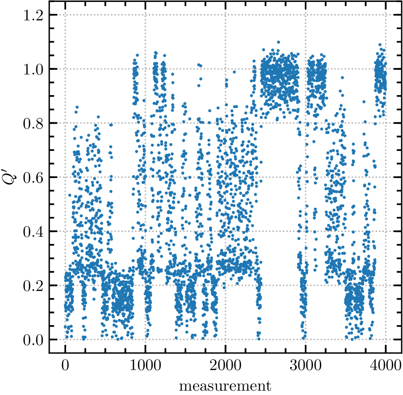
Figure 1: Piece of a Markov-chain history of $Q^{\prime}$ against measurement number for lattice B_2d. The reweighting allows efficient sampling in three regions, $0<Q^{\prime}<0.27$, $0.20<Q^{\prime}<0.85$, and $0.8<Q^{\prime}<1.05$, but has difficulty moving between these regions. The same figure is published in our paper Jahn et al. (2018).

Using the reweighting approach as developed and established in Ref. Jahn et al. (2018), we observed that there are three regions where reweighting allows for efficient sampling, while it has problems moving between those regions, as indicated in Fig. 1. The problem of those two “barriers” gets severe when we go to higher temperatures or finer lattices. Solving those problems would therefore give significantly better efficiency; the susceptibility could be determined from much shorter Markov chains. This will be important in the future, when we move from our current exploratory pure-glue, Wilson-action studies to studies including light fermions. The reason for the occurrence of the barriers is that reweighting only in terms of the topological charge is incomplete and missing some information that distinguishes between the different regions. In this paper, we address how to overcome both barriers. This leads to improved efficiency of the reweighting method and allows for a direct measurement of the topological susceptibility up to very high temperatures and fine lattices.

This paper is organized as follows: In Sec. II, we discuss in detail the modification of the original reweighting approach that significantly improves the efficiency of the method. Sec. III contains the lattice determination of the susceptibility at three temperatures, $T=2.5\,T_{\mathrm{c}}$, $4.1\,T_{\mathrm{c}}$, and $7.0\,T_{\mathrm{c}}$, each at three spacings with $N_{\tau}=10,12,14$. This allows us to check our previous results and to perform a continuum extrapolation and a power-law fit as a function of temperature. A discussion of our results can then be found in Sec. IV.

II The Method

In this section, we discuss the improvement of the reweighting method that overcomes both “barriers.” We shall refer to those barriers as the low barrier, i.e., the barrier at around $Q^{\prime}\simeq 0.25$ in Fig. 1, and the high barrier, i.e., the barrier at around $Q^{\prime}\simeq 0.85$ in Fig. 1. This section starts by addressing the origin of both problems and how to improve tunneling through the corresponding barriers. We shall find that both problems need to be solved differently and we hence have to split up the whole lattice setup into multiple distinct Monte Carlo samples. This section is concluded by a discussion of how the different Monte Carlo samples can be combined to a measurement of the topological susceptibility.

II.1 The Low Barrier

The low barrier occurs because the algorithm has problems to move between configurations with trivial topology and dislocations, i.e., small concentrations of topological charge that are the intermediate steps between the $Q=0$ and $Q=1$ sectors. For an additional reweighting, we therefore need a quantity that distinguishes between these two types of configurations. Since for dislocations the topological charge is spatially very concentrated, we expect that the action is also sharply peaked at the dislocation’s location. We therefore consider the peak action density

$$G\equiv\max_{\tilde{x}}\big{\{}S(\tilde{x})\big{\}}\,,$$ (5)

where $\tilde{x}$ denotes a point in the dual lattice and

$$S(\tilde{x})=\sum_{P(\tilde{x})}\mathrm{Re}\operatorname{tr}\mathopen{}\mathclose{{}\left(1-P(\tilde{x})}\right)$$ (6)

with $P(\tilde{x})$ being the 24 plaquettes that lie on the hypercube bounding the primitive cell with center $\tilde{x}$. We use $G$ as a quantity that distinguishes between topologically trivial configurations and dislocations. Note that, by definition,

$$\sum_{\tilde{x}}S(\tilde{x})=4\cdot S_{\mathrm{W}}\,,$$ (7)

where $S_{\mathrm{W}}$ is the Wilson gauge action.

Figure 2 shows the values of the topological charge $Q$ and this action-density measure $G$ for lattice-discretized Harrington-Shepard (HS) calorons, as a function of the caloron radius $\rho/a$ (cf. Ref. Jahn et al. (2019)). As expected, $G$ peaks at $\rho\simeq a$, i.e., for dislocations, precisely where $Q^{\prime}$ is intermediate between topology-0 and topology-1 values. On the other hand, for configurations where the caloron is so small that it falls between the lattice points, $G$ is also small; and $G$ is also small for large calorons which clearly display topological character. Therefore $G$ is a good discriminant for configurations for which topology is ambiguous.

The reason for the “low barrier” between $Q^{\prime}<0.2$ configurations and $Q^{\prime}>0.3$ configurations, seen in Figure 1, is precisely because of the difficulty in getting between non-topological configurations and ambiguous-topology configurations characterized by a large $G$ value. To see this, consider the distribution, in the $(Q^{\prime},G)$ plane, of the configurations generated by a $Q^{\prime}$-reweighted HMC Markov chain, shown in the left panel of Figure 3. There is a clear “gap” in the sample, with very few points sampling the region around $G=7$ and $Q^{\prime}=0.25$. For every $Q^{\prime}$ value between 0 and 0.5, the sample is dominated either by $G\simeq 2$ configurations or by $G\sim 11$ configurations, or by a linear combination of these two; it is never controlled by configurations intermediate between these $G$ values. The failure to sample such configurations inhibits the Markov chain’s ability to sample both parts of the configuration space.

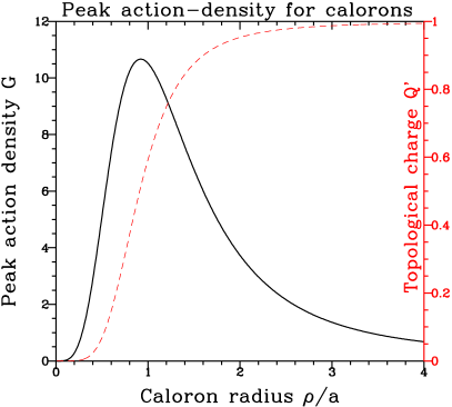
Figure 2: Left: Symanzik-improved topological charge $Q$ for Harrington-Shepard (HS) calorons as a function of caloron size. Right: peak action density $G$ for the same HS calorons (with $Q$ also shown in red). The maximum in $G$ occurs precisely where $Q$ is intermediate between 0, its $\rho=0$ value, and 1, its large-$\rho$ asymptote.

Figure 3: Distribution of topological charge $Q^{\prime}$ and peak action density $G$, obtained during a reweighted Markov chain. Left: reweighting in terms of $Q^{\prime}$ only (on an $8\times 32^{3}$ lattice at $T=4.1T_{\mathrm{c}}$). Right: reweighting in terms of both $Q^{\prime}$ and $G$ (on lattice $B_{1}$ and only extending up to $Q^{\prime}=0.6$).

To encourage transitions across this “gap,” instead of reweighting solely in terms of $Q^{\prime}$ (here renamed $Q^{\prime}_{\mathrm{L}}$ for reasons which will become clear), we perform an additional reweighting in terms of $G$. The effective reweighting function is then the sum of two individual reweighting functions:

$$W_{\mathrm{low}}(Q^{\prime}_{\mathrm{L}},G)=W_{Q}(Q^{\prime}_{\mathrm{L}})+W_{G}(G)\,.$$ (8)

Note that $G$ is also evaluated after some amount of gradient flow $t_{f,G}$ that in principle does not have to equal the flow time $t_{f,\mathrm{L}}$ after which $Q^{\prime}_{\mathrm{L}}$ is evaluated. Hand-tuning showed that the amount of gradient flow that gives the best performance depends on the size of the lattice; larger lattices need more flow. The specific choices of these parameters for our lattices are listed in Tab. 1. We also saw that HMC trajectories with one step of length $0.2\,a$ give the best performance in this region. Both reweighting functions are built simultaneously in the same way as described in detail in Ref. Jahn et al. (2018).

Reweighting in terms of both $Q^{\prime}_{\mathrm{L}}$ and $G$ removes the barrier, as seen in the right panel of Figure 3. It increases by more than a factor of 5 the number of transitions between $Q^{\prime}_{\mathrm{L}}\simeq 0$ and $Q^{\prime}_{\mathrm{L}}\simeq 0.5$ configurations, for a given number of HMC trajectories. Therefore this approach appears to cure the low barrier.

Unfortunately reweighting in terms of $G$ does not significantly help with the high barrier, as already suggested in the left panel of Figure 3. Therefore we will only use this method to perform a Monte-Carlo over a reduced range of $Q^{\prime}_{\mathrm{L}}$ values, which we will call the low region (L). Specifically, we reweight $Q^{\prime}_{\mathrm{L}}$ only up to a value $Q^{\mathrm{L}}_{\mathrm{max}}$, which we choose to be 1.15 times the $Q^{\prime}_{\mathrm{L}}$ value for the HS caloron with the maximum $G$ value, which we can look up from the right panel of Figure 2. We strictly reject configurations with $Q^{\prime}_{\mathrm{L}}>Q^{\mathrm{L}}_{\mathrm{max}}$; the role of such configurations will be covered by the middle and upper regions, which we will describe next. All values of $G$ are allowed, but our reweighting function is only nontrivial between $G_{\mathrm{min}}$ and $G_{\mathrm{max}}$, where $G_{\mathrm{min}}$ is the mean value we find in a short non-reweighted Markov chain and $G_{\mathrm{max}}$ is the largest value for the caloron solutions shown in the left panel of Figure 2. Note that configurations that are outside of this $G$-interval are not rejected; we just extend the reweighting function as a constant beyond the limits, that is, $W_{G}(G>G_{\mathrm{max}})=W_{G}(G_{\mathrm{max}})$ and $W_{G}(G<G_{\mathrm{min}})=W_{G}(G_{\mathrm{min}})$.

II.2 The High Barrier

The actual configurations carrying topology at finite temperature are expected to be nontrivial objects with large fluctuations, not “clean” HS calorons. Nevertheless, we will refer to them as calorons in what follows. We can define the “size” of such a configuration as the size of the HS caloron it approaches under gradient flow – note that, up to lattice artifacts, HS calorons are extrema of the action and do not change size under gradient flow, so gradient flow brings topological objects towards clean HS calorons. Therefore it makes logical sense to discuss the size distribution of calorons. Perturbatively we expect the dominant size to be $\rho\sim 0.5N_{\tau}a$ Jahn et al. (2019); but the size of a dislocation is closer to $\rho\sim 1.5a$. Since we want to compare the relative weight of topological and non-topological configurations, and $\rho\sim 1.5a$ configurations are a necessary intermediate step, we have to make sure that our HMC Markov chain moves efficiently across the range of caloron sizes from $\rho\sim 1.5a$ to $\rho\sim 0.5N_{\tau}a$. Our continuum extrapolation will involve $N_{\tau}=10,12,14$, so we need efficiency up to quite large calorons (in lattice units). As we understand it, the difficulty in doing so is what drives the high barrier in Figure 1.

The quantity $G$ that we introduced for the low barrier is unfortunately not helpful here, because there is no real “gap” in the $(Q^{\prime},G)$ distribution between $Q^{\prime}=0.5$ and $Q^{\prime}=1$ in the left panel of Fig. 3. Until now we were not able to find an auxiliary variable which significantly improves performance in this high region. Therefore we will have to find other ways to make this region more efficient.

The first thing to note is that the calorons under consideration are rather large and robust objects. Therefore it is no longer necessary to perform the Markov chain using short, inefficient HMC trajectories. So we switch to longer HMC trajectories (10 steps of $0.25\,a$), which induce much larger changes in our gauge field configuration. This already significantly improves efficiency in the high region.

Next, consider the variable $Q^{\prime}$ we use for reweighting. The right panel of Figure 2 shows how the $a^{2}$-improved definition of topology varies as a function of caloron size for clean, idealized HS calorons. We see that in the range of interest, $\rho\in[1.5,7]a$, $Q$ varies very little. Therefore, we need a precise determination of $Q$ if it is to prove useful in distinguishing between different caloron sizes. Unfortunately, $Q^{\prime}$ is a noisy measurable. To see why a little better, note that our lattice definition of $Q^{\prime}$ is contaminated by high-dimension operators: $q_{\mathrm{latt}}^{\prime}(x)\simeq q(x)+c_{2}a^{2}F^{a}_{\mu\nu}D^{2}\tilde{F}^{a}_{\mu\nu}+c_{4}a^{4}F^{a}_{\mu\nu}D^{4}\tilde{F}^{a}_{\mu\nu}+\ldots$. Operator improvement forces $c_{2}=0$, but higher terms still exist, and the dimension-8 operators appearing in this expansion do not integrate to topological invariants. Contributions from these high dimension operators are dominated by the shortest-distance scale which is not erased by gradient flow. Therefore, integrating up $q_{\mathrm{latt}}^{\prime}(x)$ will give the topology of the configuration, plus nontopological fluctuations which are suppressed by $\sim a^{4}/t_{f}^{2}$, but whose variance is extensive in the lattice volume. This makes it clear that a larger depth of flow can greatly suppress these fluctuations, providing a cleaner value of $Q^{\prime}$. So defining $Q^{\prime}$ using a larger amount of gradient flow leads to a cleaner variable, which is better able to distinguish between different caloron sizes. Unfortunately, a larger amount of gradient flow simply destroys dislocations, so this approach cannot be used in the low region. Therefore we will use one amount of gradient flow $t_{f,\mathrm{low}}\in[0.36,0.54]a^{2}$ to define $Q^{\prime}_{\mathrm{L}}$, which we will use in the low region, and another amount of gradient flow $t_{f,\mathrm{high}}\in[0.96,1.32]a^{2}$ to define $Q^{\prime}_{\mathrm{H}}$, which we will use in the high region. Larger lattice volumes and lower temperatures demand larger $t_{f}$ values; for the smallest lattices we consider, we choose the lower ends of the indicated ranges, while for the largest lattices we use the upper ends.

Finally, when we reweight in terms of some variable, our methodology involves choosing intervals in that variable, with $W[Q^{\prime}_{\mathrm{H}}]$ chosen as piecewise linear across each interval. Our method for determining the reweighting function $W[Q^{\prime}_{\mathrm{H}}]$ leads to approximately equal sampling of each interval. We want to sample nearly equally in $\rho$, not in $Q^{\prime}_{\mathrm{H}}$. Therefore, we choose a uniform set of $\rho$ values, from a minimum value for which $Q^{\prime}_{\mathrm{H}}=0.7\equiv Q^{\mathrm{H}}_{\mathrm{min}}$, up to a maximum value $\rho_{\mathrm{max}}=0.5N_{\tau}a$. We use the right-hand plot in Figure 2 to look up the associated $Q^{\prime}_{\mathrm{H}}$ value of each, and use these as the edges of our intervals. This leads to more sampling, and more sensitivity, at the largest $Q^{\prime}_{\mathrm{H}}$ values, corresponding to larger calorons.

The price we pay for these methodological changes is, that our procedure now differs – both in HMC trajectory choice and in reweighting variable choice – between the upper and lower regions. And as we have defined them, these regions do not necessarily even overlap. Therefore we will need a procedure for “sewing together” these regions, which we describe next.

II.3 The Middle Region

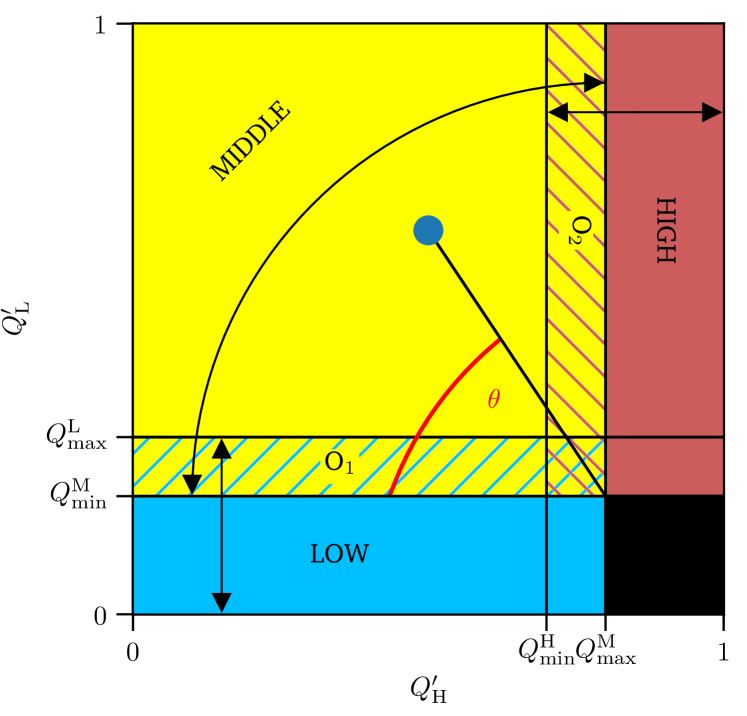
Figure 4: Visualization of the different regions: Low (blue), Middle (yellow), High (red), overlap $\mathrm{O}_{1}$ (blue hatched), and overlap $\mathrm{O}_{2}$ (red hatched). A generic configuration in the middle region is depicted by a blue point. The arrows indicate the “transitions” that should be enhanced by reweighting in the respective regions. The black region is the region where the system is simultaneously both in the high and the low region. This region is forbidden and those configurations are strictly rejected.

The middle region (M) is chosen such that it has an overlap with both the high and the low regions, while those regions are disjoint. In this region, we measure the topological charge after both flow times, i.e., we measure both $Q^{\prime}_{\mathrm{L}}$ and $Q^{\prime}_{\mathrm{H}}$. These quantities are highly correlated but still different, and the middle region aims to smoothly transition from one to the other. This then corresponds to smoothly connecting the low and high regions. The middle region is constrained by requiring $Q^{\prime}_{\mathrm{L}}>Q^{\mathrm{M}}_{\mathrm{min}}\equiv Q^{\mathrm{L}}_{\mathrm{max}}/1.15$ and $Q^{\prime}_{\mathrm{H}}<Q^{\mathrm{M}}_{\mathrm{max}}\equiv 1.15\times Q^{\mathrm{H}}_{\mathrm{min}}$, meaning that the overlap with both the high and low regions is 15%. Configurations with $Q^{\prime}_{\mathrm{L}}<Q^{\mathrm{M}}_{\mathrm{min}}$ or $Q^{\prime}_{\mathrm{H}}>Q^{\mathrm{M}}_{\mathrm{max}}$ are strictly rejected. The remaining values are reweighted according to a reweighting function which smoothly interpolates between being purely dependent on $Q^{\prime}_{\mathrm{L}}$ at $Q^{\mathrm{M}}_{\mathrm{min}}$ and being purely dependent on $Q^{\prime}_{\mathrm{H}}$ at $Q^{\mathrm{M}}_{\mathrm{max}}$. Specifically, we define the reweighting variable $\theta$ to be the angle

$$\theta=\arctan\mathopen{}\mathclose{{}\left(\frac{Q^{\prime}_{\mathrm{L}}-Q^{\mathrm{M}}_{\mathrm{min}}}{Q^{\mathrm{M}}_{\mathrm{max}}-Q^{\prime}_{\mathrm{H}}}}\right)\in\mathopen{}\mathclose{{}\left[0,\,\pi/2}\right]\,.$$ (9)

$\theta=0$ then corresponds to $Q^{\prime}_{\mathrm{L}}=Q^{\mathrm{M}}_{\mathrm{min}}$ which connects the middle region with the low region, and $\theta=\nicefrac{{\pi}}{{2}}$ corresponds to $Q^{\prime}_{\mathrm{H}}=Q^{\mathrm{M}}_{\mathrm{max}}$ which connects the middle region with the high region. The overlap regions are then defined as

$$\mathrm{O}_{1} \equiv\mathopen{}\mathclose{{}\left\{Q^{\prime}_{\mathrm{L}}\colon Q^{\mathrm{M}}_{\mathrm{min}}\leq Q^{\prime}_{\mathrm{L}}\leq Q^{\mathrm{L}}_{\mathrm{max}}}\right\}\,,$$ (10)

$$\mathrm{O}_{2} \equiv\mathopen{}\mathclose{{}\left\{Q^{\prime}_{\mathrm{H}}\colon Q^{\mathrm{H}}_{\mathrm{min}}\leq Q^{\prime}_{\mathrm{H}}\leq Q^{\mathrm{M}}_{\mathrm{max}}}\right\}\,.$$ (11)

The different regions are visualized in Fig. 4. In the middle region, using an HMC trajectory of four steps of length $0.25\,a$ turned out to give the best performance. Note that $Q^{\prime}_{\mathrm{L}}$ and $Q^{\prime}_{\mathrm{H}}$ are highly correlated, so few if any configurations lie in the lower right part of the figure; in fact, our method implicitly assumes that the black region is empty. Figure 5 shows a scatterplot of $Q^{\prime}_{\mathrm{L}}$ and $Q^{\prime}_{\mathrm{H}}$ for a reweighted Markov chain performed in this middle region, showing that the two $Q^{\prime}$ values are correlated, and that almost no configurations land in the overlap of the two overlap regions.

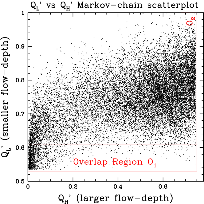
Figure 5: Scatter plot of $Q^{\prime}_{\mathrm{L}}$ against $Q^{\prime}_{\mathrm{H}}$ in a reweighted Markov chain sampling of the middle region, in a $14\times 48^{3}$ lattice at $T=7.0T_{\mathrm{c}}$. The values are strongly but imperfectly correlated, and very few points land in the overlap of $\mathrm{O}_{1}$ and $\mathrm{O}_{2}$.

The statistical power of a Monte-Carlo in this middle region improves quite quickly with the length of the Markov chain, because the reweighting proves to be modest. Therefore one can build a sample with negligible statistical errors using a fraction of the Monte-Carlo time needed on the other regions.

II.4 Reweighting with Multiple Regions

Our strategy will be to perform one independent Monte-Carlo simulation in each of the three regions. In each Monte-Carlo, we record the reweighting function $W$ and the true topology $Q$ for every tenth configuration generated by the Markov chain. Here we show how these independent Monte-Carlos can be combined to determine the topological susceptibility.

We have a sample of $Q^{\prime},W[Q^{\prime}],Q$ values from each Markov chain, and we want to use them to determine the susceptibility. As we see in Eq. (1), we need to determine $\langle Q^{2}\rangle$; because $|Q|\geq 2$ configurations are negligible, this is the same as the fraction of configurations with $Q=1$. In a single-region Monte Carlo simulation, we would determine that via

$$\mathopen{}\mathclose{{}\left\langle Q^{2}}\right\rangle \equiv\frac{\int\mathcal{D}U\>\mathrm{e}^{-\beta S[U]}\;\Theta\mathopen{}\mathclose{{}\left(Q-Q_{\mathrm{thresh}}}\right)}{\int\mathcal{D}U\>\mathrm{e}^{-\beta S[U]}}$$

$$\simeq\frac{\sum_{i}\mathrm{e}^{-W[Q^{\prime}_{i}]}\>\Theta\mathopen{}\mathclose{{}\left(Q_{i}-Q_{\mathrm{thresh}}}\right)}{\sum_{i}\mathrm{e}^{-W[Q^{\prime}_{i}]}}\,,$$ (12)

where $Q^{\prime}_{i}$ is the determined $Q^{\prime}$ value for the $i$ configuration in the sample. Here $Q_{i}$ is $|Q|$ measured on the $i$’th configuration after some (larger) depth of gradient flow, and $Q_{\mathrm{thresh}}$ is a threshold used to separate the $Q=1$ and $Q=0$ sectors. We will check later that the specific values of flow depth and threshold have almost no bearing at the lattice spacings we consider.

This approach now has to be extended for multiple regions with their own Monte Carlo samples. The key is the correct use of the overlap regions. We introduce the shorthand notation $P_{R}$ for the fraction of the total probability over all configurations, which lies in region $R$. That is,

$$P_{R}=\frac{\int\mathcal{D}U\>\mathrm{e}^{-\beta S[U]}\;\Theta[Q^{\prime}\in R]}{\int\mathcal{D}U\>\mathrm{e}^{-\beta S[U]}}\,,$$ (13)

where $\Theta[Q^{\prime}\in R]$ means that we include only those configurations which satisfy the condition to be in region $R$. Similarly, we introduce $P_{R,\,Q}$ to mean the same but with the additional requirement that $Q=1$:

$$P_{R,\,Q}=\frac{\int\mathcal{D}U\>\mathrm{e}^{-\beta S[U]}\;\Theta[Q^{\prime}\in R]\;\Theta\mathopen{}\mathclose{{}\left(Q-Q_{\mathrm{thresh}}}\right)}{\int\mathcal{D}U\>\mathrm{e}^{-\beta S[U]}}\,.$$ (14)

Defining A (“All”) to be the region containing the whole reweighting domain, we need to determine

$$\mathopen{}\mathclose{{}\left\langle Q^{2}}\right\rangle=\frac{P_{\mathrm{A},\,Q}}{P_{\mathrm{A}}}=\frac{P_{\mathrm{L},\,Q}+P_{\mathrm{M}-\mathrm{O}_{1}-\mathrm{O}_{2},\,Q}+P_{\mathrm{H},\,Q}}{P_{\mathrm{L}}+P_{\mathrm{M}-\mathrm{O}_{1}-\mathrm{O}_{2}}+P_{\mathrm{H}}}\,,$$ (15)

where we used that $\mathrm{A}=\mathrm{L}\cup\mathopen{}\mathclose{{}\left(\mathrm{M}-\mathrm{O}_{1}-\mathrm{O}_{2}}\right)\cup\mathrm{H}$ and by $\tilde{M}\equiv\mathrm{M}-\mathrm{O}_{1}-\mathrm{O}_{2}$ we mean all points in the middle region with both overlap regions removed. Note that this corresponds to removing the region $\mathrm{O}_{1}\cap\mathrm{O}_{2}$ twice, i.e., $\tilde{M}$ contains all points in the middle region that are in neither of the two overlap regions with weight $+1$, the disjoint parts of the two overlap regions with weight $0$, and the common part of the overlap regions, i.e., $\mathrm{O}_{1}\cap\mathrm{O}_{2}$, with weight $-1$. Eq. (15) can be rewritten as

$$\mathopen{}\mathclose{{}\left\langle Q^{2}}\right\rangle =\frac{P_{\mathrm{H},\,Q}}{P_{\mathrm{L}}}\times\mathopen{}\mathclose{{}\left(\frac{P_{\mathrm{L},\,Q}+P_{\mathrm{M}-\mathrm{O}_{1}-\mathrm{O}_{2},\,Q}+P_{\mathrm{H},\,Q}}{P_{\mathrm{H},\,Q}}}\right)$$

$$\phantom{=\frac{P_{\mathrm{H},\,Q}}{P_{\mathrm{L}}}}\ \times\mathopen{}\mathclose{{}\left(\frac{P_{\mathrm{L}}+P_{\mathrm{M}-\mathrm{O}_{1}-\mathrm{O}_{2}}+P_{\mathrm{H}}}{P_{\mathrm{L}}}}\right)^{-1}$$

$$\equiv\Xi_{0}\cdot\Xi_{1}\cdot\Xi_{2}^{-1}\,.$$ (16)

Using the overlap regions, each of those terms can be rewritten as

$$\Xi_{0} \equiv\frac{P_{\mathrm{H},\,Q}}{P_{\mathrm{L}}}=\frac{P_{\mathrm{H},\,Q}}{P_{\mathrm{O}_{2}}}\times\frac{P_{\mathrm{O}_{2}}}{P_{\mathrm{O}_{1}}}\times\frac{P_{\mathrm{O}_{1}}}{P_{\mathrm{L}}}\,,$$ (17a)

$$\Xi_{1} \equiv\frac{P_{\mathrm{L},\,Q}+P_{\mathrm{M}-\mathrm{O}_{1}-\mathrm{O}_{2},\,Q}+P_{\mathrm{H},\,Q}}{P_{\mathrm{H},\,Q}}$$

$$\begin{split}&=1+\mathopen{}\mathclose{{}\left(\frac{P_{\mathrm{M}-\mathrm{O}_{1}-\mathrm{O}_{2},\,Q}}{P_{\mathrm{O}_{2}}}\times\frac{P_{\mathrm{O}_{2}}}{P_{\mathrm{H},\,Q}}}\right)\\ &\phantom{=1}\ +\mathopen{}\mathclose{{}\left(\frac{P_{\mathrm{L},\,Q}}{P_{\mathrm{O}_{1}}}\times\frac{P_{\mathrm{O}_{1}}}{P_{\mathrm{O}_{2}}}\times\frac{P_{\mathrm{O}_{2}}}{P_{\mathrm{H},\,Q}}}\right)\,,\end{split}$$ (17b)

$$\Xi_{2} \equiv\frac{P_{\mathrm{L}}+P_{\mathrm{M}-\mathrm{O}_{1}-\mathrm{O}_{2}}+P_{\mathrm{H}}}{P_{\mathrm{L}}}$$

$$\begin{split}&=1+\mathopen{}\mathclose{{}\left(\frac{P_{\mathrm{M}-\mathrm{O}_{1}-\mathrm{O}_{2}}}{P_{\mathrm{O}_{1}}}\times\frac{P_{\mathrm{O}_{1}}}{P_{\mathrm{L}}}}\right)\\ &\phantom{=1}\ +\mathopen{}\mathclose{{}\left(\frac{P_{\mathrm{H}}}{P_{\mathrm{O}_{2}}}\times\frac{P_{\mathrm{O}_{2}}}{P_{\mathrm{O}_{1}}}\times\frac{P_{\mathrm{O}_{1}}}{P_{\mathrm{L}}}}\right)\,,\end{split}$$ (17c)

where now each ratio is determined by a single Monte Carlo simulation in the high region, middle region, or low region.

We expect that almost all of the total weight of configurations is in the low region, while almost all of the total weight of $Q=1$ configurations lies in the high region. Consequently, we expect that $\Xi_{1}\approx 1\approx\Xi_{2}$. Naturally we shall check this; but to the extent that it holds, we obtain the easier expression

$$\mathopen{}\mathclose{{}\left\langle Q^{2}}\right\rangle\approx\Xi_{0}=\frac{P_{\mathrm{H},\,Q}}{P_{\mathrm{O}_{2}}}\times\frac{P_{\mathrm{O}_{2}}}{P_{\mathrm{O}_{1}}}\times\frac{P_{\mathrm{O}_{1}}}{P_{\mathrm{L}}}\,.$$ (18)

Under this approximation, we end up with a product of three ratios, each of which can be determined using a single one of our Monte Carlo samples:

$$\frac{P_{\mathrm{H},\,Q}}{P_{\mathrm{O}_{2}}} =\frac{\sum_{i\in\mathrm{H}}\>\mathrm{e}^{-W_{\mathrm{high}}\mathopen{}\mathclose{{}\left[Q^{\prime}_{\mathrm{H}}}\right]}\;\Theta\mathopen{}\mathclose{{}\left(Q-Q_{\mathrm{thresh}}}\right)}{\sum_{i\in\mathrm{H}}\>\mathrm{e}^{-W_{\mathrm{high}}\mathopen{}\mathclose{{}\left[Q^{\prime}_{\mathrm{H}}}\right]}\;\Theta\mathopen{}\mathclose{{}\left(Q^{\prime}_{\mathrm{H}}\in\mathrm{O}_{2}}\right)}\,,$$ (19)

$$\frac{P_{\mathrm{O}_{2}}}{P_{\mathrm{O}_{1}}} =\frac{\sum_{i\in\mathrm{M}}\>\mathrm{e}^{-W_{\mathrm{mid}}\mathopen{}\mathclose{{}\left[\theta}\right]}\;\Theta\mathopen{}\mathclose{{}\left(Q^{\prime}_{\mathrm{H}}\in\mathrm{O}_{2}}\right)}{\sum_{i\in\mathrm{M}}\>\mathrm{e}^{-W_{\mathrm{mid}}\mathopen{}\mathclose{{}\left[\theta}\right]}\;\Theta\mathopen{}\mathclose{{}\left(Q^{\prime}_{\mathrm{L}}\in\mathrm{O}_{1}}\right)}\,,$$ (20)

$$\frac{P_{\mathrm{O}_{1}}}{P_{\mathrm{L}}} =\frac{\sum_{i\in\mathrm{L}}\>\mathrm{e}^{-W_{\mathrm{low}}\mathopen{}\mathclose{{}\left[Q^{\prime}_{\mathrm{L}}\,,G}\right]}\;\Theta(Q^{\prime}_{\mathrm{L}}\in\mathrm{O}_{1})}{\sum_{i\in\mathrm{L}}\>\mathrm{e}^{-W_{\mathrm{low}}\mathopen{}\mathclose{{}\left[Q^{\prime}_{\mathrm{L}}\,,G}\right]}}\,.$$ (21)

Therefore, within our approximations, we can easily determine all three ratios. And we need all three Monte Carlos, because each determines one of these three ratios.

II.5 Parameters to Tune

As in the original reweighting approach, we still find that a certain amount of hand-tuning is required to achieve the best efficiency of our method. First, there are the depths of gradient flow to use in establishing the reweighting variables $Q^{\prime}_{\mathrm{L}}$, $G$, and $Q^{\prime}_{\mathrm{H}}$. We find that in the high region a rather large amount of gradient flow is required to carefully distinguish calorons of different sizes. In the low region, we need to tune both $t_{f,\mathrm{low}}$ and $t_{f,G}$, and it is not clear that both flow depths should be the same. In particular, $t_{f,G}$ needs to be enough flow that fluctuations are removed, but too much flow shrinks the dislocations and the peak action density cannot distinguish between trivial topology and dislocations any more. Similar arguments hold for $t_{f,\mathrm{low}}$. We find that $t_{f,\mathrm{low}}$ slightly larger than $t_{f,G}$ improves the efficiency, but a more careful analysis would be desirable, especially in view of the inclusion of fermions. This could be done by carefully comparing the peak action density of discretized calorons and thermal configurations after different amounts of gradient flow.

Second, there is the position of the lower bound of the high region. We chose $Q^{\mathrm{H}}_{\mathrm{min}}=0.7$ throughout because this choice definitely includes the high barrier for all lattices we consider. Changing $Q^{\mathrm{H}}_{\mathrm{min}}$ affects the sampled regions for both the middle and high analyses, and will impact the statistical power of each Monte-Carlo in opposite directions. It might be worth revisiting what value is optimal overall.

Next, there is the length of the HMC trajectories used in the respective regions. We chose the lengths such the the acceptance rate of the reweighting Metropolis step is about 50%; this leads to small trajectories in the low region, large trajectories in the high region, and to intermediate-sized trajectories in the middle region. Again, a more careful analysis could still improve the efficiency of the algorithm by comparing the achieved statistics at fixed numerical effort as a function of the HMC trajectory lengths in the respective regions.

Finally, there is the definition of the topological charge as the observable for determining the topological susceptibility. Since we saw in Ref. Jahn et al. (2018) that the continuum extrapolated results are insensitive to the exact choices of both the flow depth and the threshold, we use $t_{f}=2.4\,a^{2}$ of Wilson flow and $Q_{\mathrm{thresh}}=0.7$ for deciding whether a configuration is topological or not throughout this section, in accordance with the choices in Ref. Jahn et al. (2018). This allows us to directly compare our results to the ones obtained with the original reweighting approach. We will investigate other choices to ensure that our final answers are not dependent on this choice.

III Results

Table 1: The lattices used in this section. The lattices labeled with “A” correspond to simulations at $2.5\,T_{\mathrm{c}}$, the lattices labeled with “B” correspond to $4.1\,T_{\mathrm{c}}$, and the lattices labeled with “C” are simulations at $7\,T_{\mathrm{c}}$. We also indicate the amount of gradient flow that was used in the definitions of each reweighting variable.

Lat	$T/T_{\mathrm{c}}$	$\phantom{a}N_{\tau}\phantom{a}$	$N_{x}\times N_{y}\times N_{z}$	$\beta_{\mathrm{lat}}$	$t_{f,\mathrm{low}}/a^{2}$	$t_{f,G}/a^{2}$	$t_{f,\mathrm{high}}/a^{2}$
$\text{A}_{1}$	2.5	10	$36\times 32^{2}$	$6.90097$	$0.48$	$0.42$	$0.96$
$\text{A}_{2}$	2.5	12	$40\times 36^{2}$	$7.04966$	$0.48$	$0.48$	$0.96$
$\text{A}_{3}$	2.5	14	$48^{3}$	$7.17706$	$0.54$	$0.48$	$1.32$
$\text{B}_{1}$	4.1	10	$36\times 32^{2}$	$7.30916$	$0.42$	$0.42$	$0.96$
$\text{B}_{2}$	4.1	12	$40\times 36^{2}$	$7.46275$	$0.48$	$0.48$	$0.96$
$\text{B}_{3}$	4.1	14	$48^{3}$	$7.59354$	$0.48$	$0.48$	$1.32$
$\text{C}_{1\mathrm{a}}$	7.0	10	$12^{3}$	$7.76294$	$0.36$	$0.36$	$0.96$
$\text{C}_{1\mathrm{b}}$	7.0	10	$16^{3}$	$7.76294$	$0.36$	$0.36$	$0.96$
$\text{C}_{1\mathrm{c}}$	7.0	10	$24^{3}$	$7.76294$	$0.42$	$0.42$	$0.96$
$\text{C}_{1\mathrm{d}}$	7.0	10	$32^{3}$	$7.76294$	$0.42$	$0.42$	$0.96$
$\text{C}_{1\mathrm{e}}$	7.0	10	$40^{3}$	$7.76294$	$0.48$	$0.48$	$0.96$
$\text{C}_{2}$	7.0	12	$40\times 36^{2}$	$7.91939$	$0.48$	$0.48$	$0.96$
$\text{C}_{3}$	7.0	14	$48^{3}$	$8.05216$	$0.48$	$0.48$	$1.32$

Our goal is to demonstrate that the improved reweighting method as described above yields statistically powerful results in a range of lattice spacings and volumes and allows for the determination of the topological susceptibility up to $7.0\,T_{\mathrm{c}}$ in the quenched approximation, where the original reweighting approach from Ref. Jahn et al. (2018) is limited due to the barriers described above. To crosscheck our results, we also determine the susceptibility again at $2.5\,T_{\mathrm{c}}$ and $4.1\,T_{\mathrm{c}}$. We already saw in the original approach that at such high temperatures it is sufficient to only take into account the $Q=1$ sector because the higher topological sectors are too suppressed to significantly contribute to the topological susceptibility. We therefore only reweight the $Q=1$ sector as discussed in the previous section.

First we investigate the dependence of the susceptibility on the lattice aspect ratio. It is known Braaten and Nieto (1995) that the long-distance correlations of Yang-Mills theory well above $T_{\mathrm{c}}$ are described by a 3D theory with correlation lengths which are parametrically of order $1/gT$ and $1/g^{2}T$. This implies that, for all temperatures $T\gg T_{\mathrm{c}}$, an aspect ratio which is parametrically $\mathcal{O}(1/g^{2})$ should be sufficient; there is no need to keep the physical volume fixed as we increase the temperature. Since $1/g^{2}$ is largest for the highest temperature, we then study the aspect ratio dependence at $T=7T_{\mathrm{c}}$ and we assume that a ratio which is sufficient at this temperature will also work at the lower temperatures. We show the resulting susceptibility as a function of aspect ratio, all at $N_{\tau}=10$, in Figure 7. The results indicate that aspect ratios above about 2.4 show no discernible volume dependence. Therefore we conservatively choose aspect ratios somewhat above 3 in all other cases.

To carry out the continuum extrapolation we will consider lattice spacings with $N_{\tau}=10,\,12,\,14$ at each temperature we explore. We adopt the scale-setting (the relation between the lattice spacing $a$ and inverse coupling $\beta_{\mathrm{latt}}$) determined in Burnier et al. (2017). In total, we study 13 different lattice setups as listed in Tab. 1. All calculations were conducted over a three month period on the Lichtenberg high performance computer center of the TU Darmstadt and on one server node with four 16-core Xeon Gold CPUs. Because some machines had 24-core nodes, we made some unusual choices of lattice sizes such that at least one lattice direction would be a multiple of 12.

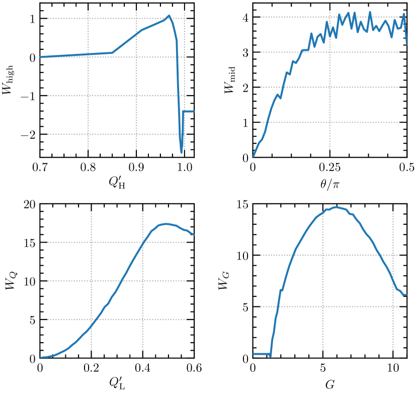
Figure 6: Reweighting functions for a $14\times 48^{3}$ lattice at $7\,T_{\mathrm{c}}$ (Lattice C₃). The reweighting function in the low region is the sum of the two reweighting functions in the low panels, i.e., $W_{\mathrm{low}}(Q^{\prime}_{\mathrm{L}},G)=W_{Q}(Q^{\prime}_{\mathrm{L}})+W_{G}(G)$.

The first task is to build the four reweighting functions that are needed to completely sample one of the lattices. In total, we therefore have 52 different reweighting functions. One example of these functions for a $14\times 48^{3}$ lattice at $7\,T_{\mathrm{c}}$ is shown in Fig. 6. The reweighting function $W_{\mathrm{high}}$ looks, as expected, like the high-$Q^{\prime}$ part of the reweighting function in the original reweighting approach. It shows a very narrow minimum around $Q^{\prime}_{\mathrm{H}}=1$, corresponding to genuine $Q=1$ calorons. At smaller $Q^{\prime}_{\mathrm{H}}$, the reweighting function shows a plateau corresponding to dislocations. Moving from a genuine caloron to a dislocation requires a reweighting of only about $\mathrm{e}^{-3}$ which is the reason that at lower temperatures and coarser lattices, where the barrier gets even smaller, no reweighting is needed at all to efficiently sample the high region. The reweighting function $W_{\mathrm{mid}}$ samples between dislocations of different sizes and the function shows a monotonically increasing trend. The “spikes” result from the fact that we discretized the $\theta$ domain with 50 intervals; a smaller number would have been sufficient. However, the reweighting needed to sample this region is only $\mathrm{e}^{-4}$ and due to the “simple” monotonically increasing form of the reweighting function and the small structural differences between the relevant configurations, the middle region is sampled very efficiently. The low region is sampled with the sum of the two reweighting functions $W_{Q}$ and $W_{G}$. The topological-charge reweighting function $W_{Q}$ has a deep minimum at $Q^{\prime}_{\mathrm{L}}=0$, corresponding to ordinary, topologically trivial $Q=0$ configurations. The function then increases until a maximum is reached that corresponds to dislocations. Note that reaching the dislocations requires a large amount of reweighting of roughly $\mathrm{e}^{-18}$. The peak action-density reweighting function $W_{G}$ shows a large maximum at intermediate $G$ which corresponds to the “gap” in the right panel of Fig. 2. Moving through this gap therefore requires a large amount of reweighting of roughly $\mathrm{e}^{-15}$.

With these reweighting functions at hand, we proceed to determine the topological susceptibility via Eqs. (1) and (18). Since we saw in the original reweighting approach that it does not affect the results if we use Wilson or Zeuthen flow, we only use the computationally slightly cheaper Wilson flow here. For deciding whether a configuration is topological or not, we measure the topological charge after $t_{f}=2.4\,a^{2}$ Wilson flow, thresholded with $Q_{\mathrm{thresh}}=0.7$. We will present a check on this procedure at the end of this section.

The first question is whether the approximations proposed in Eq. (18) are justified. For this, we tested the validity of our approximations by explicitly measuring $\Xi_{1}$ and $\Xi_{2}$ on lattices $\mathrm{A}_{\mathrm{1}}$ and $\mathrm{C}_{\mathrm{2}}$. The result is

$$\mathopen{}\mathclose{{}\left|1-\Xi_{1}^{\mathrm{A}_{1}}}\right|\equiv 0\equiv\mathopen{}\mathclose{{}\left|1-\Xi_{1}^{\mathrm{C}_{2}}}\right|$$ (22)

meaning that there is not a single caloron in the middle and low regions. Also the second approximation is fulfilled very precisely:

$$\mathopen{}\mathclose{{}\left|1-\mathopen{}\mathclose{{}\left(\Xi_{2}^{\mathrm{A}_{1}}}\right)^{-1}}\right| \approx 3.2\times 10^{-4}\,,$$ (23)

$$\mathopen{}\mathclose{{}\left|1-\mathopen{}\mathclose{{}\left(\Xi_{2}^{\mathrm{C}_{2}}}\right)^{-1}}\right| \approx 3.6\times 10^{-9}\,.$$ (24)

That is, all but a tiny fraction of the total weight in the ensemble is contained in configurations in the low region. We therefore proceed using Eq. (18) for determining the topological susceptibility. For completeness, we present all our results in Tab. 2.

Table 2: Number of measurements (with 10 HMC trajectories per measurement), number of times the Markov chain moved from the top to the bottom of each range and back, and the final determined susceptibility for each lattice listed in Table 1.

Lat	#Measurements			#Complete sweeps			$\ln\mathopen{}\mathclose{{}\left(\chi_{\mathrm{top}}/T_{\mathrm{c}}^{4}}\right)$
	L	M	H	L	M	H
$\text{A}_{1}$	$175{,}560$	$40{,}680$	$53{,}820$	536	861	805	$-8.11(09)$
$\text{A}_{2}$	$139{,}690$	$16{,}670$	$62{,}980$	464	491	554	$-8.23(12)$
$\text{A}_{3}$	$182{,}460$	$24{,}790$	$56{,}760$	665	626	592	$-8.47(10)$
$\text{B}_{1}$	$237{,}960$	$32{,}440$	$61{,}120$	768	593	970	$-11.41(09)$
$\text{B}_{2}$	$337{,}540$	$16{,}940$	$71{,}530$	479	453	625	$-11.63(11)$
$\text{B}_{3}$	$167{,}990$	$21{,}410$	$59{,}030$	490	549	526	$-11.83(12)$
$\text{C}_{1\mathrm{a}}$	$100{,}000$	$100{,}000$	$66{,}400$	83	$2{,}215$	$1{,}915$	$-16.88(30)$
$\text{C}_{1\mathrm{b}}$	$100{,}000$	$100{,}000$	$74{,}200$	105	$2{,}450$	$1{,}822$	$-16.17(13)$
$\text{C}_{1\mathrm{c}}$	$321{,}700$	$26{,}300$	$24{,}200$	269	454	385	$-15.12(14)$
$\text{C}_{1\mathrm{d}}$	$368{,}420$	$21{,}630$	$84{,}800$	483	655	$1{,}353$	$-15.11(08)$
$\text{C}_{1\mathrm{e}}$	$307{,}300$	$15{,}800$	$41{,}700$	422	382	636	$-14.97(10)$
$\text{C}_{2}$	$487{,}240$	$32{,}080$	$54{,}420$	490	931	496	$-15.22(11)$
$\text{C}_{3}$	$268{,}220$	$20{,}360$	$60{,}920$	462	475	531	$-15.45(12)$

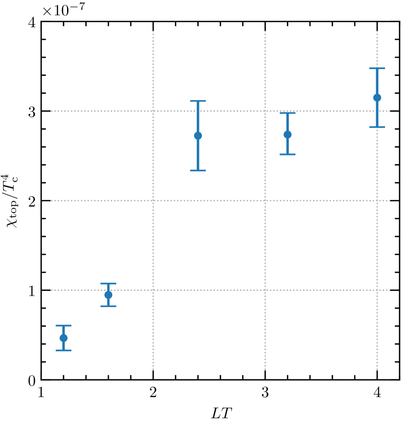
Figure 7: Finite volume dependence of the topological susceptibility $\chi_{\mathrm{top}}$ at $N_{\tau}=10$ and $T=7.0\,T_{\mathrm{c}}$ (Lattices C_1a through C_1e).

Figure 8: Continuum extrapolation in terms of the logarithm of the topological susceptibility $\chi_{\mathrm{top}}$ for the three temperatures. Left: $2.5\,T_{\mathrm{c}}$. We additionally show the results from the original reweighting approach Jahn et al. (2018). Middle: $4.1\,T_{\mathrm{c}}$. Right: $7\,T_{\mathrm{c}}$, using the lattices C_1d, C₂, and C₃. We additionally show the results with flow time $t_{f}=18.0\,a^{2}$. The points with dashed error bars are the continuum-extrapolated results.

We now consider the volume dependence by studying $\chi_{\mathrm{top}}$ as a function of the aspect ratio at $7\,T_{\mathrm{c}}$ with $N_{\tau}=10$, using lattices C_1a through C_1e. This is presented in Fig. 7. In agreement with the corresponding result in the original reweighting approach, aspect ratios smaller than 2 are badly discrepant, while aspect ratios larger than about 2.5 give consistent results and the large-volume behavior is reached. For determining the continuum extrapolation of the topological susceptibility, we therefore use aspect ratios between 3 and 3.5.

Finally, we address the continuum extrapolation of the topological susceptibility at three temperatures $2.5\,T_{\mathrm{c}}$, $4.1\,T_{\mathrm{c}}$, and $7.0\,T_{\mathrm{c}}$, using three lattice spacings for each temperature with $N_{\tau}=10,\,12,\,14$. As already elaborated in the discussion of the continuum extrapolation of the original reweighting approach, the continuum extrapolation is conducted in terms of the logarithm of the susceptibility, i.e., we linearly extrapolate $\ln\mathopen{}\mathclose{{}\left(\chi_{\mathrm{top}}}\right)$ against $a^{2}$. The continuum extrapolations of the three different temperatures are presented in Fig. 8. At $T=2.5\,T_{\mathrm{c}}$ (left panel of Fig. 8), we additionally show the results with $t_{f}=2.4\,a^{2}$ Wilson flow from the original reweighting approach. This clearly shows that lattices with $N_{\tau}=6$ are too coarse to be in the scaling region, while the finer lattices with $N_{\tau}=8$ and $N_{\tau}=10$ are consistent with the continuum extrapolation. To explicitly check that the continuum extrapolated results do not depend on the depth of gradient flow used for determining the topological charge, we additional show the results for a much larger depth of flow, $t_{f}=18.0\,a^{2}$, in the $T=7.0\,T_{\mathrm{c}}$ continuum extrapolation (right panel of Fig. 8). In accordance with our findings in Ref. Jahn et al. (2018), the different $Q$ definitions are nearly indistinguishable at finer lattices ($N_{\tau}=12,14$), while the difference becomes larger at coarser lattices ($N_{\tau}=10$). However, the continuum extrapolated results differ only by about 6%, despite the very different flow times.

IV Discussion

We presented an extension of the reweighting technique developed in Ref. Jahn et al. (2018) that improves the efficiency in determining the topological susceptibility in pure SU(3) Yang-Mills theory. The method is based on the individual treatment of the topologically trivial sector $Q=0$ (“low region”), the topological $Q=1$ sector (“high region”), and the intermediate dislocations with fractional $0<Q<1$ (“middle region”). In the low region, a combined reweighting in terms of the topological charge and the peak action density, both evaluated at a small amount of gradient flow, allows to efficiently sample between topologically trivial configurations and dislocations. Since this requires a large amount of reweighting and the involved topological objects are small and fragile, only very small HMC trajectories (one step of $0.2\,a$) can be used; otherwise the acceptance rate in the reweighting step becomes very small. In the high region, sampling between genuine calorons and dislocations requires only a small amount of reweighting. Since also the involved topological objects are large and robust, large HMC trajectories (eight steps of $0.25\,a$) allow for an efficient sampling. At coarser lattices ($N_{\tau}=10,\,12$), no reweighting is necessary at all in this region; at finer lattices ($N_{\tau}=14$), a large amount $t^{\prime}_{\mathrm{H}}=1.32\,a^{2}$ of Wilson flow allows for a careful distinction of calorons of different sizes. In the middle region, sampling between dislocations with different sizes requires only a small amount of reweighting and using intermediate-size HMC trajectories (four steps of $0.25\,a$) allows for a very efficient sampling.

This method is very effective and allows for a continuum-extrapolated determination of the topological susceptibility up to the very high temperature $T=7.0\,T_{\mathrm{c}}$ and up to an aspect ratio of 4 and fine lattice spacings with $N_{\tau}=14$; this determination constitutes the first direct measurement of the susceptibility at such a high temperature. Our final results are

$$\begin{split}\chi_{\mathrm{top}}(T=2.5\,T_{\mathrm{c}})&=1.52\times 10^{-4}\ \mathrm{e}^{\pm 0.22}\,T_{\mathrm{c}}^{4}\,,\\ \chi_{\mathrm{top}}(T=4.1\,T_{\mathrm{c}})&=4.84\times 10^{-6}\ \mathrm{e}^{\pm 0.24}\,T_{\mathrm{c}}^{4}\,,\\ \chi_{\mathrm{top}}(T=7.0\,T_{\mathrm{c}})&=1.51\times 10^{-7}\ \mathrm{e}^{\pm 0.23}\,T_{\mathrm{c}}^{4}\,.\end{split}$$ (25)

To emphasize again how important reweighting is to a direct determination of $\chi(T=7.0\,T_{\mathrm{c}})$, note that without reweighting, $Q=1$ configurations in our finest-spacing, highest-temperature lattice would represent approximately $3\times 10^{-9}$ of all configurations. Because there is also a large autocorrelation time to jump from $Q=1$ back to $Q=0$ configurations, it would take at least $10^{10}$ HMC updates to observe any topological configurations, and $\sim 10^{12}$ HMC updates to gather comparable statistics to what we achieve with $3\times 10^{6}$ HMC updates. Therefore, to obtain the susceptibility at such temperatures, either our reweighting method or an indirect method such as the approach of Borsanyi et al Borsanyi et al. (2016b) must be used.

The continuum-extrapolated results for $2.5\,T_{\mathrm{c}}$ and $4.1\,T_{\mathrm{c}}$ are consistent within errors with the corresponding results from the original reweighting approach Jahn et al. (2018) and hence also with the literature Borsanyi et al. (2016a); Berkowitz et al. (2015). Applying the grand continuum fit of Ref. Borsanyi et al. (2016a), also the continuum extrapolated result at $7\,T_{\mathrm{c}}$ agrees well with their findings.

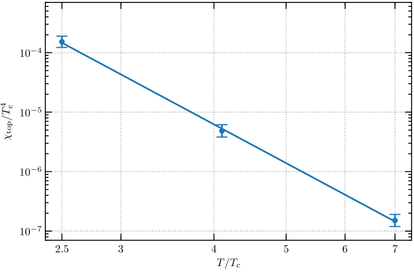
Figure 9: Continuum extrapolated results of the topological susceptibility as a function of temperature in a double-logarithmic plot. We also show the simple power-law fit Eqs. (26) and (27).

The continuum extrapolated results are plotted against temperature in a double-logarithmic plot in Fig. 9. A perturbative prediction of the temperature dependence of the topological susceptibility at high temperatures in the framework of the dilute instanton gas approximation Gross et al. (1981) suggests that the continuum extrapolated data may be fitted in the form

$$\frac{\chi_{\mathrm{top}}}{T_{\mathrm{c}}^{4}}=\frac{\chi_{\mathrm{top}}^{0}}{T_{\mathrm{c}}^{4}}\mathopen{}\mathclose{{}\left(\frac{T}{T_{\mathrm{c}}}}\right)^{b}$$ (26)

which has a linear behavior in a double logarithmic plot. The best fit parameters of our continuum extrapolated results are

$$\ln\mathopen{}\mathclose{{}\left(\frac{\chi_{\mathrm{top}}^{0}}{T_{\mathrm{c}}^{4}}}\right)=-2.67(46)\,,\qquad b=-6.72(31)\,,$$ (27)

where the uncertainties are statistical only. In pure SU(3) Yang-Mills theory, the dilute instanton gas approximation predicts the exponent $b=-7$ which is consistent with our result. In a recent study, Borsanyi et al. also determined this exponent in a conventional heat-bath/overrelaxation setup Borsanyi et al. (2016a). Despite applying much more numerical effort, they have significantly larger statistical errors and only reach $4\,T_{\mathrm{c}}$; but their result $b=-7.1(4)$ is consistent with ours. In their determination, Berkowitz et al. found the result $b=-5.64(4)$ Berkowitz et al. (2015) which differs significantly from our result. However, they only reached $2.5\,T_{\mathrm{c}}$, which may be too low to display the same slope as in the regime we study.

This methodology can be applied in a straightforward way to the full (unquenched) theory. However, the $Q=0$ and $Q=1$ sectors differ in that the former will have no small fermionic eigenvalues, while the latter will; this may require a careful handling of the fermionic mass, and the use of fermionic implementations with excellent chirality properties. We leave the application of our methodology to the full theory for future work.