Additional Calibration of the Ultra-Violet Imaging Telescope on board AstroSat

Abstract

Results of the initial calibration of the Ultra-Violet Imaging Telescope (UVIT) were reported earlier by Tandon et al. (2017a). The results reported earlier were based on the ground calibration as well as the first observations in orbit. Some additional data from the ground calibration and data from more in-orbit observations have been used to improve the results. In particular, extensive new data from in-orbit observations have been used to obtain (a) new photometric calibration which includes (i) zero-points (ii) flat fields (iii) saturation, (b) sensitivity variations (c) spectral calibration for the near Ultra-Violet (NUV; 2000$-$3000 Å) and far Ultra-Violet (FUV; 1300$-$1800 Å) gratings, (d) point spread function and (e) astrometric calibration which includes distortion. Data acquired over the last three years show continued good performance of UVIT with no reduction in sensitivity in both the UV channels.

1 Introduction

Ultra-Violet Imaging Telescope (UVIT) is one of the five payloads on board the Indian multi-wavelength astronomy satellite AstroSat (Agrawal, 2006). Four of the five instruments on AstroSat observe in the soft and hard X-ray bands, while UVIT observes in the Ultra-Violet bands. The primary aim of UVIT is simultaneous imaging in the far Ultra-Violet (FUV; 1300$-$1800 Å) and the near Ultra-Violet (NUV; 2000$-$3000 Å) channels over a field of $\sim$28^′ diameter with a spatial resolution $<$ 1.5^′′. For both FUV and NUV channels, multiple filters are provided for observations in a narrower band, and options for slit-less spectroscopy, with a resolution of $\sim$80, too are provided. The initial calibration of UVIT was reported in Tandon et al. 2017a, (hereinafter referred to as Paper-1), which were based on the measurements done on ground and initial observations on the sky. With accumulation of in-orbit observations carried out over about 30 months on the calibration fields, the calibration has been refined and the results are reported here. These results supersede the ones reported in Paper-1. The paper is organised as follows: important details of the instrument are described in Section 2, a brief description of the calibration reported in Paper-1 is presented in Section 3, details of the new observations are given in Section 4, results of the calibration are given in Section 5 and Section 6 is devoted to conclusions.

Table 1: Key parameters of the three channels of UVIT

Parameter	FUV	NUV	VISa
Wavelength (Å)	1300 $-$ 1800	2000 $-$ 3000	3200 $-$ 5500
Mean Wavelengthb (Å)	1481	2418	4200
Mean Effective Area (cm2)	$\sim$10	$\sim$40	$\sim$50
Field of view (diameter - arcmin)	28	28	28
Plate Scale ($\prime\prime$/pixel)	3.33	3.33	3.30
Astrometric accuracy (rms)	0.4′′	0.4′′
Zero-point magnitudec	18.1	19.8
Spatial resolutiond (FWHM)	1.3′′ $-$ 1.5′′	1.2′′ $-$ 1.4′′	2.5′′
Spectral resolutione (Å)	17	33
Saturation (counts/sec)f (10%)	6	6

Note. — ^a For the VIS channel all the parameters are based on ground calibration. This channel is operated in integration mode. Photometric calibration is not done as we don’t expect doing science with VIS channel observations. This channel is meant for aspect correction.

^b The mean wavelength is for the filter with maximum bandwidth, and is obtained by weighting wavelengths with the corresponding effective area as measured in calibration on the ground.

^c The zero point magnitude (for the filter with maximum bandwidth) is in AB system and refers to the average flux of HZ4 in the band

^d It depends on perturbations in the pointing.

^e These are for the gratings.

^f The saturation is given for the full field images. These are taken at a rate 28.7 frames/s; images for partial field are taken at higher frequency of the frames and the range of linearity is higher

2 Instrumentation

Two co-aligned Ritchey-Chretien telescopes, each of aperture $\sim$375 mm, are used to image in FUV (1300$-$1800 Å), NUV (2000$-$3000 Å) and VIS (3200$-$5500 Å) channels. As drift in the pointing can be many arc-seconds at rates up to 2 arc-second/sec, images are generated by combining short-exposure frames ($<<$ 1 sec) after applying corrections for drift. Many of the fields would not have enough flux in NUV/FUV for tracking the drift, therefore images taken with the VIS channel, at regular intervals of $\sim$1 sec, are used to monitor the drift. Each of the three channels has a filter wheel to select a narrower band for imaging. For low resolution slit-less spectroscopy, one grating is provided in the NUV wheel and two gratings (with orthogonal dispersions) are provided in the FUV wheel. Intensified CMOS imagers, of aperture 39 mm, are used for all the three channels. The imagers can work either in photon-counting mode (with high intensification/high electron multiplication due to high voltage in the micro channel plate; MCP) or in integration mode (with low intensification/low electron multiplication due to low voltage in MCP). The CMOS imagers have 512 $\times$ 512 pixels, and each of these pixels is mapped to 8 $\times$ 8 sub-pixels in the final image to get a plate-scale of $\sim$0.416^′′ per sub-pixel. Observations can be carried out for the full field of $\sim$28^′ diameter, at a rate $\sim$29 frames/sec or for a selectable partial field at a higher rate. Key performance parameters of the three channels are presented in Table 1, and properties of the filters are shown in Table 2. For more details of the instrument the reader is referred to Tandon et al. (2017b) and the references therein.

Table 2: Properties of the individual filters of UVIT. Here, $\lambda_{mean}$ is the mean wavelength (estimated by weighting the wavelengths with the effective areas) and $\Delta\lambda$ is the band width (between the wavelengths with effective area 50% of the peak) .

Filter Name	Filter	$\lambda_{mean}$ (Å)	$\Delta\lambda$ (Å)
F148W	CaF2-1	1481	500
F148Wa	CaF2-2	1485	500
F154W	BaF2	1541	380
F172M	Silica	1717	125
F169M	Sapphire	1608	290
N242W	Silica-1	2418	785
N242Wa	Silica-2	2418	785
N245M	NUVB13	2447	280
N263M	NUVB4	2632	275
N219M	NUVB15	2196	270
N279N	NUVN2	2792	90
V347M†	VIS1	3466	400
V391M	VIS2	3909	400
V461W	VIS3	4614	1300
V420W	BK7	4200	2200
V435ND	ND1	4354	2200

Note. — ^† The VIS channel is only meant for aspect correction and not expected for science observation. The inbuilt safely features of UVIT require the count rates in VIS channel not to exceed 4800 c/s for any individual point source. To enable observations of fields that have optical sources with varied brightness levels, the VIS channel too have different filters such as V347M, V391M, V461W, V420W and V435ND.

3 Calibration required

All the calibration can be divided into four sets (see Paper-1 for details). The scope of these is briefly described below

1. Photometric calibration: This includes (a) zero point magnitudes at the centre of the field for different filters obtained from the observations on a standard star (HZ 4 is observed for this), (b) flat-field variations remaining after correcting for variations in the sensitivity of the detectors as observed in the ground calibration at the mean wavelengths, and (c) correction for saturation in the photon-counting mode.

2. Monitoring sensitivity of FUV and NUV channels: As throughput of the FUV and NUV channels can be reduced by depositions of contaminants on the optics, as well as due to ageing of the filters, the MCPs and coatings on the mirrors, sensitivity of both the channels is monitored every few months.

3. Spectral calibration for the NUV and FUV gratings: This includes (a) effective area as a function of wavelength, (b) dispersion, and (c) resolution.

4. Point Spread Function, including encircled energy as a function of radius.

5. Astrometric calibration giving estimates of errors in the positions after correcting for distortions in the detectors as per the ground calibration.

The results of calibration were earlier reported in Paper-1. With the availability of more data from in orbit observations, improved results, particularly on the flat field variations have been obtained, and are presented in Section 5.

4 Observations and Data Analysis

The results reported here are based on the observations of HZ 4, three overlapping fields in the Small Magellanic Cloud (SMC) and NGC 188. All the observations were made in photon-counting mode of the detectors. Most of the observations were made with full field, but some of the observations for HZ 4 were made with partial field to get frame rates up to $\sim$292 frames/sec to minimise the effect of saturation. More details for the observations can be found in Paper-1. To monitor any possible reduction in throughput of FUV and NUV channels, due to deposition of any contaminants on the optics or due to ageing of the filters and the MCPs, a field in NGC 188 was selected as its high declination provides visibility throughout the year. The three fields in SMC were selected as follows: the first field was selected away from the centre of SMC to avoid the brightest part, the other two fields were selected to get shifts of $\sim$6^′ in two orthogonal directions with reference to the first field. The shifts of $\sim$6^′ were used to get a good overlap between the fields as well as obtain a separation of several arcminutes for positions of common objects in the three images. The differences in count-rates between the three positions provide data on differential sensitivity across more than one thousand separation-vectors distributed over the area of the detector. All the images were generated with CCDLAB (Postma & Leahy, 2017). In CCDLAB, each event is corrected for position as well as flat-field. The positions are corrected for: (i) a bias called fixed pattern noise, (ii) distortion, and (iii) drift of the pointing. The correction for flat-field is only for the spatial variations in sensitivity of the detectors as measured during pre-launch calibration, i.e. possible contributions of other optical elements are not included and are to be deduced from these images as discussed under ”Remainders of flat field” in Section 5.1.3. The corrections for distortion were generated by a reanalysis of all data from ground calibration done at the University of Calgary and at the Indian Institute of Astrophysics (IIA), and have small differences compared to what were used for the results reported in Paper-1. The arrays for flat-field corresponding to the pre-launch calibration, too were regenerated by correcting the position of each event for distortion on the detector, which is equivalent to correcting for errors due to variations in plate-scale caused by distortions, and have small differences compared to what were used for the results reported in Paper-1. Filters F148Wa and N242Wa are spare filters which were not used for any observations and hence no results are presented for these.

Table 3: Normalised counts/sec and zero point magnitudes for the different UVIT filters

Name	Filter	$\lambda_{mean}$ Å	Normalised	ZP magnitude
			c/s for HZ 4	Value	error
F148W	CaF2-1	1481	23.52	18.097	0.010
F154W	BaF2	1541	20.68	17.771	0.010
F169M	Sapphire	1608	16.16	17.410	0.010
F172M	Silica	1717	5.460	16.274	0.020
N242W	Silica-1	2418	127.800	19.763	0.002
N219M	NUVB15	2196	7.360	16.654	0.020
N245M	NUVB13	2447	36.97	18.452	0.005
N263M	NUVB4	2632	27.16	18.146	0.010
N279N	NUVN2	2792	5.37	16.416	0.010

Table 4: Results of ground calibration on effective areas of the filters as a function of wavelength for the centre of the field. Wavelength($\lambda$) is in Å and effective area (E) is in square cm .

F148W		F154W		F169M		F172M		N242W		N219M		N245M		N263M		N279N
$\lambda$	E	$\lambda$	E	$\lambda$	E	$\lambda$	E	$\lambda$	E	$\lambda$	E	$\lambda$	E	$\lambda$	E	$\lambda$	E
1250	0	1340	0.00	1420	0.0	1620	0.70	1700	4.08	1937	0.01	2148	0.39	2462	0.11	2705	0.10
1270	12.11	1360	4.89	1440	0.28	1650	3.65	1750	2.36	2000	0.80	2191	0.40	2496	12.12	2712	0.19
1300	12.11	1400	13.15	1480	11.25	1670	6.62	1823	0.68	2001	1.56	2209	1.21	2497	10.15	2719	0.17
1360	11.88	1440	11.95	1540	11.69	1700	8.62	1879	1.28	2009	2.04	2221	2.23	2498	13.80	2728	0.47
1400	11.98	1480	11.69	1600	10.06	1720	9.57	1937	1.97	2019	2.40	2235	3.44	2499	15.49	2733	0.98
1440	10.36	1540	12.44	1650	10.17	1750	7.02	2000	6.41	2047	3.72	2275	14.54	2500	17.45	2739	2.53
1480	11.70	1650	11.42	1700	9.14	1770	7.18	2030	27.65	2056	6.75	2282	16.30	2502	19.28	2741	3.74
1540	13.29	1700	10.28	1750	6.34	1800	1.84	2067	51.97	2065	7.14	2289	17.84	2504	22.51	2743	5.47
1600	11.61	1750	7.16	1780	2.74	1830	0.00	2138	53.61	2074	7.74	2294	19.61	2536	38.61	2745	7.46
1650	11.78	1800	0.00	1800	0.00			2214	56.25	2087	8.14	2301	21.37	2551	40.24	2746	8.89
1700	10.58							2296	58.01	2114	10.82	2308	23.13	2602	41.07	2747	10.40
1750	7.37							2385	59.11	2124	11.06	2313	25.33	2649	38.28	2748	12.00
1800	0.00							2461	56.09	2133	11.52	2320	26.66	2703	35.97	2749	14.64
								2499	55.47	2147	11.98	2369	37.13	2752	29.31	2750	14.38
								2537	54.76	2159	12.44	2381	39.26	2797	11.85	2751	17.06
								2550	54.29	2191	13.72	2388	40.95	2798	10.30	2752	19.27
								2600	51.90	2202	13.72	2400	42.65	2800	7.95	2754	21.47
								2650	46.61	2216	12.99	2409	44.14	2802	6.18	2756	23.29
								2700	43.07	2232	12.76	2440	44.90	2805	5.13	2759	25.02
								2750	35.01	2284	11.79	2452	46.31	2846	0.00	2761	25.88
								2800	30.10	2295	11.27	2466	47.72			2764	26.74
								2850	23.32	2311	10.48	2485	48.53			2770	27.42
								2900	16.93	2319	9.17	2506	48.72			2778	24.01
								2950	11.36	2367	0.76	2520	49.91			2786	24.22
								3000	7.15	2382	0.25	2541	49.63			2794	24.06
								3050	5.04	2395	0.25	2560	49.82			2799	23.61
										2410	0.25	2569	49.98			2803	23.08
												2576	45.74			2807	22.48
												2579	42.95			2813	22.17
												2581	40.53			2819	22.54
												2584	35.70			2822	23.13
												2586	32.54			2826	18.14
												2588	30.31			2830	17.68
												2591	26.58			2835	15.19
												2593	21.01			2838	12.17
												2595	18.03			2840	10.22
												2598	17.11			2842	8.20
												2600	13.76			2845	5.95
												2602	9.11			2849	3.75
												2605	7.81			2852	2.48
												2607	6.51			2856	1.38
												2609	5.02			2867	0.62
												2616	3.16			2874	0.32
												2619	1.86			2882	0.18
												2633	0.50			2889	0.09
												2656	0.33			2897	0.09
												2685	0.15
												2711	0.00

5 Results of Calibration

5.1 Photometric calibration

All the calibration mentioned in Section 3 have been redone with more in-orbit observations. There are no surprises in the new results, but in many cases these show small but significant differences.

5.1.1 Zero point magnitudes

Results of all the observations on HZ 4 have been used to recalculate zero point magnitudes for the filters. This magnitude is a measure of the sensitivity and its meaning is explained in the following sentences. Take a source which has a spectral shape identical to HZ 4 and which gives one count per second at the centre of the field, after applying all the corrections. The average flux, within band of the filter, for this source would correspond to zero point magnitude at “$\lambda_{mean}$ (see Paper-1 for more details). For any filter, the observed count rates are first corrected to get equivalent ”Normalised counts/sec” at the centre of the field by applying corrections for flat-field (including those reported below as “Remainders of flat field”), saturation (see section 5.1.4), and counts in the extended pedestal of PSF (see Table 12). The normalised counts/sec were used to calculate the zero point magnitude. To derive zero point (ZP) magnitude, an estimate is required for the average flux within band of the filter. In Paper-1, the average flux for HZ 4 was calculated within half power wavelengths of the filter, but here the full band of the filter (as shown in Table 4) is used for this calculation. The results are shown in Table 3. The errors shown correspond to 1$\sigma$ for the observed counts. Any errors related to correction for saturation and flat-field for any off-sets from the centre are expected to be no more than 1% for all the filters except N219M for which these could be 2%.

5.1.2 Effective areas

The zero point magnitudes can be interpreted quantitatively only with reference to the spectral-shapes of the filters and the calibration source. Therefore, in order to fit any model spectral energy distribution to the observed c/s in the various filters, effective areas are required as a function of wavelength (see for example Poole et al. 2008). These effective areas were calibrated on ground (see Paper-1) and are shown in Table 4. The in-orbit calibration with HZ 4 were used to estimate corrections for the areas under the assumption that relative change in transmission is independent of wavelength for each filter. These corrections are shown in Table 5. The corrected effective area is obtained by multiplying any entry in Table 4 with the corresponding entry in Table 5.

5.1.3 Remainders of flat field

During the flat-field calibration on ground, only spatial variations in sensitivity of the detectors, at 1500 Å for the FUV detector and at 2100 Å for the NUV detector, were included and these were used for processing of the images. While the beam used for these calibration was expected to be uniform over small scales, e.g. over $\sim$10^′, it could have had variations over large scales. In addition, there could be spatial variations due to other optical elements, e.g. filters, and wavelength dependent variation in sensitivity of the detectors. In order to get a direct measure of the overall flat-field, exposures were taken for three fields in SMC. The first field was selected in a suitable part of SMC ($\alpha_{2000}$ = 01:09:46, $\delta_{2000}$ = $-$71:20:30). The second field was selected by applying a shift of $\sim$6^′ in one direction, and the third field was selected by applying the shift along an orthogonal direction. These provided data for finding count rates, for a large number of sources, at three positions on the detector. The variations in these signals with position are called remainders of flat-field. Limited results on the remainders were reported in Paper-1.

Table 5: The correction for the effective areas of the filters .

Filter	Correction
Filter	F148W	F154W	F169M	F172M	N242W	N219M	N245M	N263M	N279N
Correction	0.779	0.787	0.876	0.892	0.814	0.540	0.805	0.824	0.848

Table 6: Parameters of the fit to the reminders for all the filters .

Parameter	FUV-ALL	N242W	N219M	N245M	N263M	N279N
a1	3.15 $\times$ 10-6	2.181$\times$10-5	-1.506 $\times$10-5	9.25 $\times$10-6	1.741$\times$10-5	4.09$\times$10-6
a2	-2.879 $\times$ 10-5	-1.55 $\times$10-6	1.85 $\times$10-6	1.14 $\times$10-6	-5.46 $\times$10-6	1.492$\times$10-5
a3	3.00 $\times$ 10-9	1.034$\times$10-8	9.541 $\times$10-8	1.379$\times$10-8	1.188$\times$10-8	2.151$\times$10-8
a4	-2.51 $\times$ 10-9	1.760$\times$10-8	6.761 $\times$10-8	1.188$\times$10-8	1.436$\times$10-8	2.261$\times$10-8
a5	3.30 $\times$ 10-9	5.19 $\times$10-9	2.917 $\times$10-8	2.66 $\times$10-9	6.75 $\times$10-9	1.517$\times$10-8
a6	-9.98 $\times$ 10-12	-3.63 $\times$10-12	-3.39 $\times$10-12	5.69 $\times$10-13	-4.46 $\times$10-12	3.01$\times$10-12
a7	1.232 $\times$ 10-11	4.71 $\times$10-12	1.572 $\times$10-11	6.18 $\times$10-12	1.103$\times$10-11	1.159$\times$10-11
a8	7.39 $\times$ 10-12	3.86 $\times$10-12	2.186 $\times$10-11	3.45 $\times$10-12	6.61 $\times$10-12	8.33$\times$10-12
a9	-8.32 $\times$ 10-12	-1.175$\times$10-11	1.750 $\times$10-11	1.95 $\times$10-13	-6.27 $\times$10-12	-1.96$\times$10-12
a10	2.205 $\times$ 10-5	9.905$\times$10-5	-6.51 $\times$10-6	4.001$\times$10-5	2.899$\times$10-5	3.885$\times$10-5
a11	-1.0635 $\times$ 10-4	-2.54 $\times$10-6	1.835 $\times$10-5	-5.29 $\times$10-7	-2.468$\times$10-5	1.664$\times$10-5
a12	-4.90 $\times$ 10-6	-1.327$\times$10-5	6.826 $\times$10-5	2.87 $\times$10-6	4.98 $\times$10-6	-4.747$\times$10-5
a13	4.03 $\times$ 10-6	1.73 $\times$10-6	5.165 $\times$10-5	2.00 $\times$10-6	-2.937$\times$10-5	-5.632$\times$10-5
a14	-6.772 $\times$ 10-5	1.988$\times$10-5	3.2888$\times$10-4	3.837$\times$10-5	8.167$\times$10-5	1.3243$\times$10-4

The flat-fields obtained on the ground are a good measure of small scale variations in sensitivity of the detectors. Therefore, the remainders are only expected over scales larger than $\sim$10 arcmin. The beam at the filters is $\sim$3.3 mm in diameter and any variations in the transmission on scales $<$ $\sim$1 mm are not of much consequence. In the ground calibration, all the filters except N219M gave $<$ 5% peak-to-peak variations in transmission on scales $>$ 1 mm. Therefore we considered a third order polynomial in x & y as a good choice to model the remainders, even if it misses some small scale variations for N219M. In order to avoid errors related to drifting in and out of the sources near the edges, only data for sources falling within a radius of 1900 sub-pixels were used, i.e. an extrapolation would be required to find remainders for radii $>$ 1900 sub-pixels. It was noted that a fit restricted to data for radii $<$ 1500 sub-pixels gave very small values for the remainders. But a fit for all the radii gave much larger values for the remainders for radii $<$ $\sim$1500 sub-pixels. This suggested that the relatively larger values at the outer parts of the field were biasing the fit for the central part. Therefore, the fit was made in two parts: (i) a third order polynomial for radii $<$ 1500 sub-pixels, and (ii) the change beyond radius of 1500 sub-pixels as linear in radius with four parameters to generate the azimuthal dependence. The function, $f$ a multiplicative factor, normalised to one at the centre, is written as

$$f(x,y)=1+a_{1}x+a_{2}y+a_{3}x^{2}+~{}~{}~{}~{}~{}~{}~{}~{}~{}~{}~{}~{}~{}~{}~{}~{}~{}~{}$$

$$a_{4}y^{2}+a_{5}xy+a_{6}x^{3}+a_{7}y^{3}+~{}~{}~{}~{}~{}~{}~{}~{}~{}~{}$$

$$a_{8}yx^{2}+a_{9}xy^{2};forR\leq 1500~{}~{}~{}~{}~{}~{}~{}~{}~{}~{}$$ (1)

$$f(x,y)=1+a_{1}x+a_{2}y+~{}~{}~{}~{}~{}~{}~{}~{}~{}~{}~{}~{}~{}~{}~{}~{}~{}~{}~{}~{}~{}~{}~{}~{}~{}~{}~{}~{}~{}~{}~{}~{}~{}~{}~{}~{}~{}~{}~{}~{}~{}$$

$$(1500/R)^{2}(a_{3}x^{2}+a_{4}y^{2}+a_{5}xy)+~{}~{}~{}~{}~{}~{}~{}~{}~{}~{}~{}~{}~{}~{}~{}~{}~{}~{}~{}~{}$$

$$(1500/R)^{3}(a_{6}x^{3}+a_{7}y^{3}+a_{8}yx^{2}+a_{9}xy^{2})+~{}~{}~{}~{}~{}~{}~{}~{}~{}~{}$$

$$(R-1500)(a_{10}y/R+a_{11}x/R+a_{12}*2xy/R^{2}+~{}~{}~{}~{}~{}~{}~{}~{}~{}~{}$$

$$a_{13}(x^{2}-y^{2})/R^{2}+a_{14}),forR>1500~{}~{}~{}~{}~{}~{}~{}~{}~{}~{}~{}~{}~{}~{}~{}~{}~{}~{}~{}~{}~{}~{}~{}~{}~{}$$ (2)

where x/y are the coordinates in sub-pixels as referred to the centre, and R is the radius. As direct data on the sensitivity as a function of position were not available, an approximation was used. The observed count-rates for a source at different positions can be related to differentials in sensitivity as follows:

$$(f(x1,y1)/f(x2,y2))-1=(s(x1,y1)/s(x2,y2))-1$$ (3)

$$f(x1,y1)-f(x2,y2)=(s(x1,y1)/s(x2,y2)-1)*f(x2,y2)$$ (4)

Here, s(x,y) is the sensitivity at x,y. As long as “f” does not differ much from unity , Equation 4 can be approximated as

$$f(x1,y1)-f(x2,y2)\sim s(x1,y1)/s(x2,y2)-1$$ (5)

This procedure has three possible sources of error: (i) those due to finite statistics of the measured counts of individual objects and temporal variation of some sources (ii) those due to the approximation as per Equation 5, and (iii) due to any inadequacy in the choice of the function. Based on simulations, the errors due to the finite statistics are estimated to be $<$ 2% within a radius of 12^′ and $<$ 5% for the full field, and errors due to the approximation are estimated to be $<$ 1% for all the filters except N219M (the fitted values of “$f$” for all the filters except N219M range within 0.86 and 1.18). However, for N219M, the fitted values of “$f$” range within 1 and 1.5, and the errors would be $>>$ 1%. Therefore, two iterations have been used for this filter where Equation 4 was used in the second iteration with the values of “$f$” obtained in the first iteration. The maximum values of “$f$” obtained in the first and second iterations are 1.41 and 1.49 respectively, and errors in the final values of “$f$” arising due to the approximation are estimated as $<$ 4%. All the filters for FUV are crystaline and are not expected to deteriorate in orbit. The data for all the FUV filters were combined to get a common fit called FUV-ALL. The parameters obtained for all filters are given in Table 6. These fits were applied to the counts obtained for HZ 4, with F148W, N219M, and N279N, at multiple locations on the detectors. The results suggest that the remainders are corrected to better than 5% for radii $<$ 12^′ ($\sim$1770 sub-pixels) on the detectors. This gives confidence in the process used. The actual fit was made for radii $<$ 1900 sub-pixels, but the relations for radii $>$ 1500 sub-pixels can be used up to radii of 2000 sub-pixels. The number of source pairs used for the fits are: $\sim$8000 for FUV, $\sim$4000 for N242W, $\sim$1700 for N219M, $\sim$3100 for N245M, and $\sim$1400 for N279N. Only those sources were included which had $>$ 200 counts in at least one of the two fields. As maximum possible coverage was required over the area, all the sources were given equal weight irrespective of the counts. Images taken with filter N219M (NUV B15), which shows the largest variation in sensitivity across the field of view, were analysed to check the errors at radii between 1900 and 2000 sub-pixels. A comparision of the corrected (as per the fit for radii $>$ 1500 sub-pixels) counts in images of SMC1, SMC2, and SMC3 shows that the fractional rms errors are $\sim$0.06, a major part of which could be from Poisson statistics of the counts and errors of photometry near the edge.

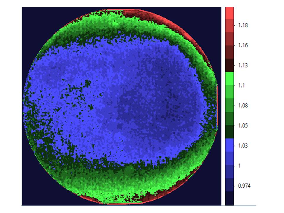
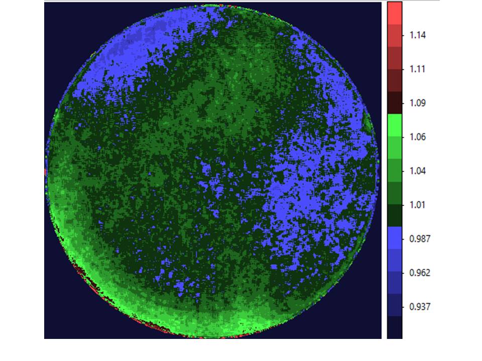
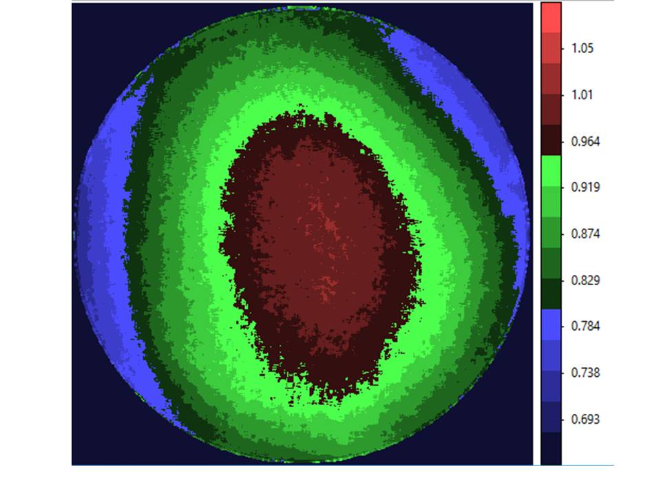
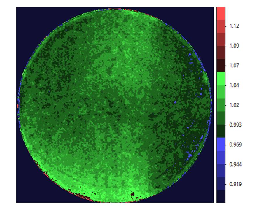
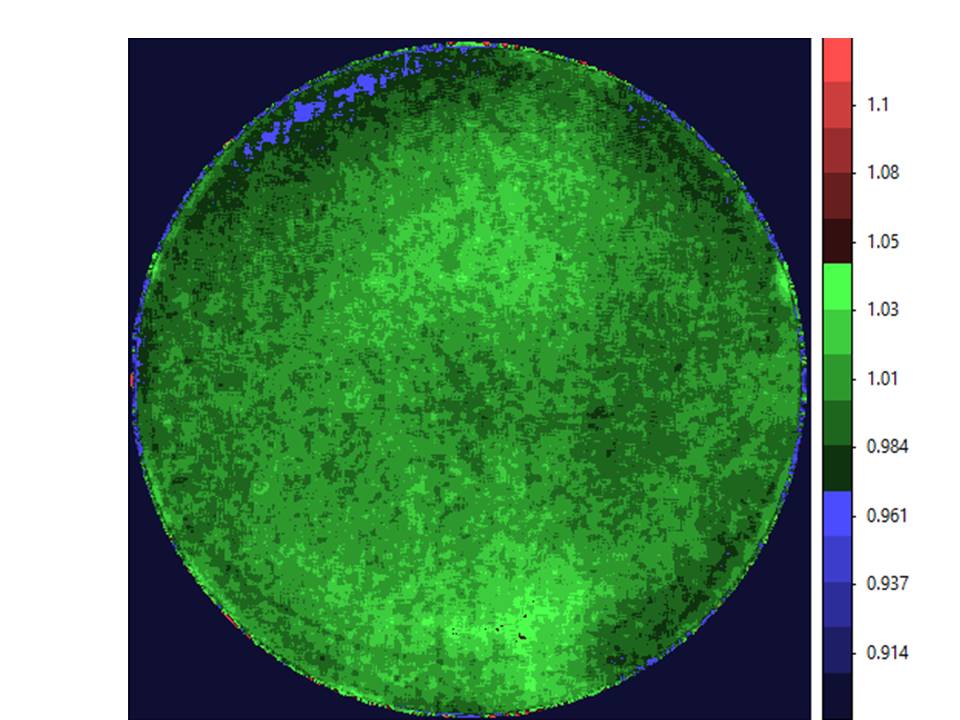
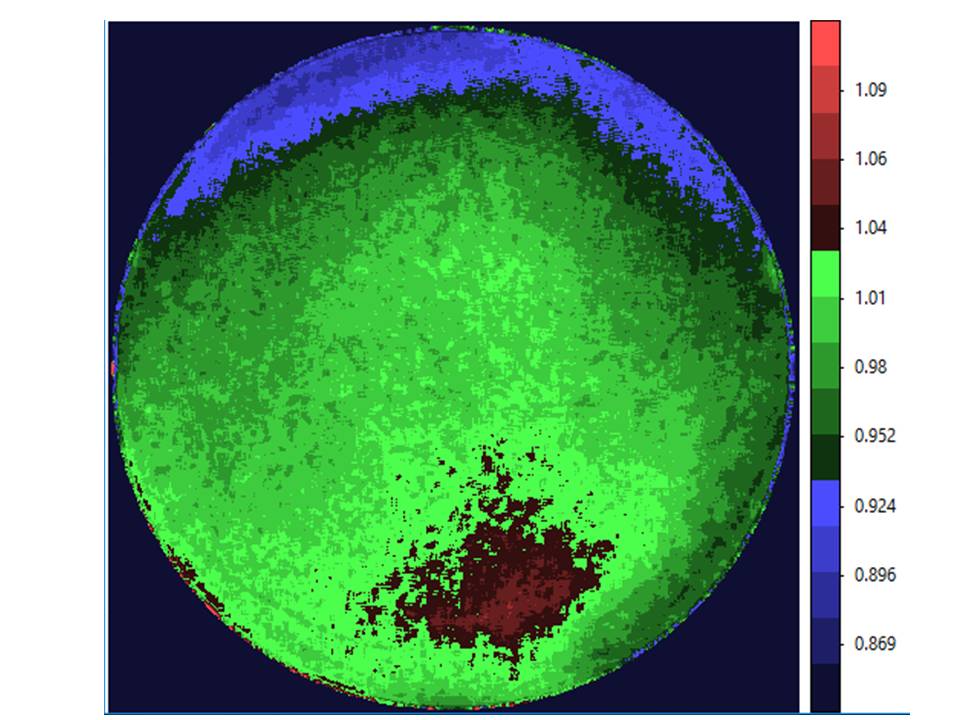
Figure 1: Overall variations for inverse of sensitivity. The panels are: Top left: All FUV filters, Top right: N242W, Middle left: N219M, Middle right: N245M, Bottom left: N263M , and Bottom right: N279N

Overall variations for inverse of the sensitivity are shown in Figure 1. These variations were obtained by combining flat-fields of the detectors measured in the ground calibration with the results obtained here for remainders of flat-field, and were normalized to one at the centre. We give in Table 7 two sets of maximum and minimum of the inverse of sensitivity over the field for different filters, one for radii $<$ 1900 sub-pixels and the other for radii $<$ 2000 sub-pixels.

Table 7: Range in the inverse of sensitivity for different filters

Filter	radii $<$ 1900 sub-pixels		radii $<$ 2000 sub-pixels
	Min.	Max.	Min.	Max.
FUV(all filters)	0.96	1.18	0.96	1.19
N219M	0.72	1.03	0.68	1.03
N242W	0.95	1.09	0.95	1.09
N245M	0.96	1.08	0.96	1.08
N263M	0.95	1.05	0.95	1.05
N279N	0.88	1.07	0.86	1.08

Table 8: Log of observations of NGC 188 in the filters F148W and N279N

	Exposure Time (secs)
Date	F148W	N279N
31/12/2015	551.6	560.4
13/07/2016	—	265.2
30/01/2017	1194.7	1202.3
16/04/2017	—	400.7
21/12/2017	148.6	157.0
22/02/2018	2893.5	1862.1
04/04/2018	430.9	—
20/07/2018	400.2	—
26/08/2018	255.2	—
13/09/2018	1163.3	—
21/09/2018	1140.4	—
23/10/2018	1140.3	—

5.1.4 Correction for saturation

In photon-counting mode, occurrence of multiple photon events in close proximity (within 3 $\times$ 3 pixels) in a frame is recorded as single photon. Therefore, there is some saturation unless the average photon rate per frame is $<<$ 1. Process of correcting this remains the same as was reported in Paper-1, and it is described below.

The actual counts per frame can be calculated by using relation of Poissonian statistics between the actual counts per frame and fraction of the frames with no count. However, as the actual PSF is spread beyond 3 $\times$ 3 sub-pixels, we have to use an empirical procedure described below. Let “CPF5” be 97% of the observed counts per frame and let “ICPF5” be the corresponding actual counts per frame as per Poissonian statistics. The equations used to get the correction for counts per frame are

$$CPF5=(1-exp(-ICPF5))$$ (6)

$$ICORR=(ICPF5)-(CPF5)$$ (7)

$$RCORR=ICORR*(0.89-0.30*(ICORR)^{2})$$ (8)

where, ICORR is the ideal correction for saturation, RCORR is the real correction. It is found that 97% of the total counts are contained within a window of radius $\sim$29 sub-pixels ($\sim$12^′′) which can be used to estimate “CPF5” in the above equations (see Section 5.4 on PSF). The parameters in the above equations are found empirically and it works well for point sources with observed (uncorrected) rates $<$$\sim$0.6 counts/frame. A similar correction for extended sources is more involved and is not discussed here. As the observed frames for a point source fall in two categories, i.e. either with one photon or with no photon, the errors on actual counts are calculated as per Binomial distribution.

5.2 Reduction in Sensitivity of UVIT

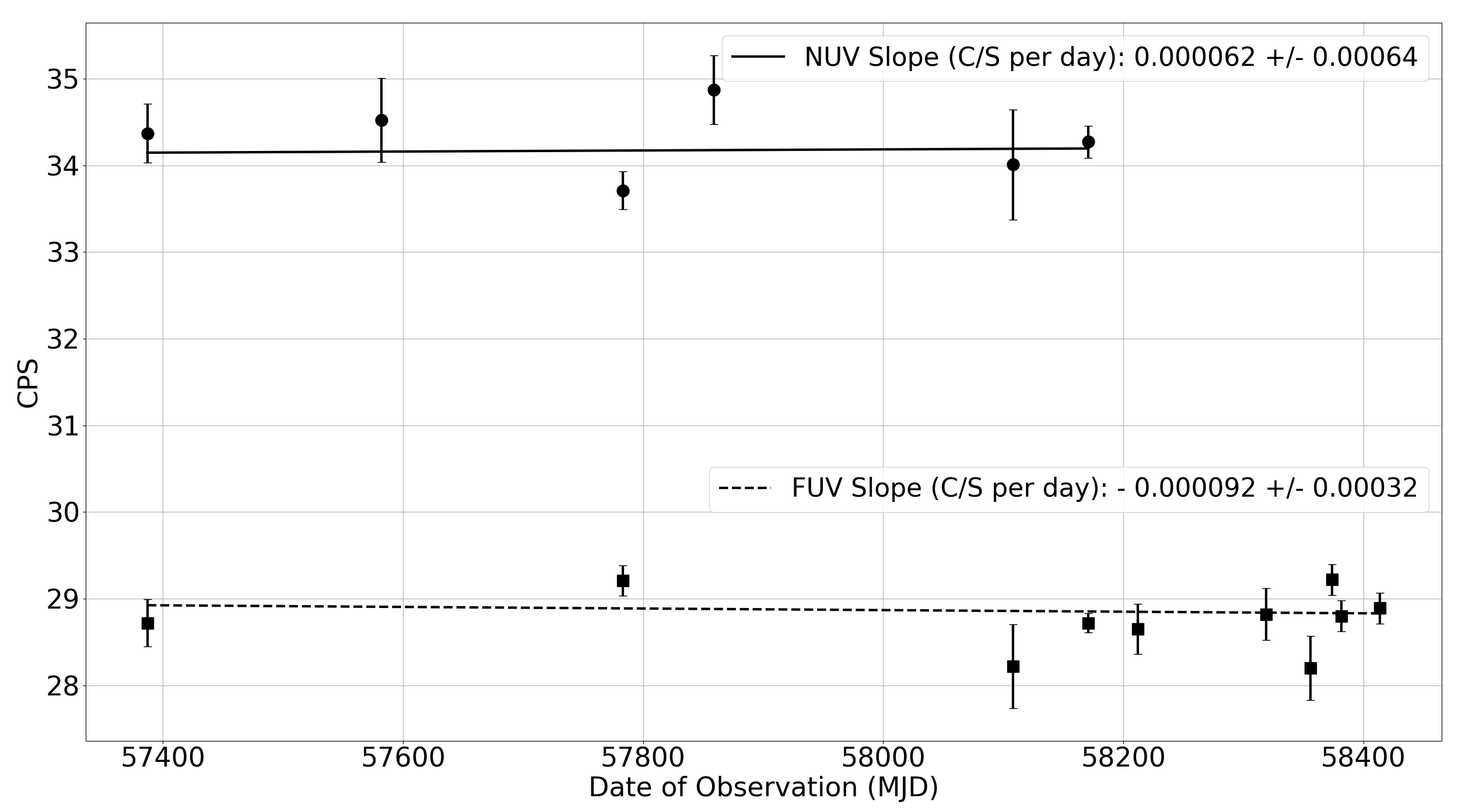
Figure 5: Variations in the sensitivity of FUV and NUV channels of UVIT between December 2015 to October 2018

During all the manoeuvres, care was taken to keep bright earth and sun away from the field of view of UVIT, but scattered Ultra-Violet radiation from these sources could lead to slow deposition of contaminants (Noter et al., 1993) on the optics and hence could lead to a reduction in sensitivity of FUV and NUV channels. In addition to this, factors such as the ageing of the MCPs and filters, interaction of radiation with the coatings on the optics could also lead to a reduction in the sensitivity of UVIT. To estimate any degradation in the sensitivity of UVIT, signals for two stars in the field of NGC 188 were tracked between December 31, 2015 to October 23, 2018. In FUV the observations were carried out in F148W filter, while in NUV, the filter N279N was used. The log of observations of NGC 188 is given in Table 8. In NUV, the two stars centered at ($\alpha_{2000}$ = 00:48:18.91, $\delta_{2000}$ = +85:13:26.04), ($\alpha_{2000}$ = 00:42:43.68, $\delta_{2000}$ = +85:14:12.48) were used, while in FUV the two stars used for tracking the reduction in sensitivity are located at ($\alpha_{2000}$ = 00:48:18.91, $\delta_{2000}$ = +85:13:26.04) and ($\alpha_{2000}$ = 00:47:52.15, $\delta_{2000}$ = +85:19:08.04) respectively. The average saturation corrected counts/sec (obtained over a circular aperture of 50 sub-pixels radius, that encompasses more than 98% of the energy in both FUV and NUV) of the two stars in FUV and NUV are given in Fig. 5. Our results are consistent with no reduction in the sensitivity of FUV and NUV channels of UVIT.

5.3 Spectroscopic Calibration

Spectroscopic calibration has been done with observations of NGC40 (for dispersion) and HZ 4 (for effective areas). The data have been reanalysed by Dewangan (2019). The results of this analysis are presented here. For typical images with the gratings and other details please refer to Paper-1. We note that in Paper-1: (i) the ”pixels” are twice in linear size as compared to the sub-pixels used here, (ii) the nomenclature for the gratings FUV1 and FUV2 is inverted relative to the nomenclature used here.

5.3.1 Dispersion and Spectral Resolution

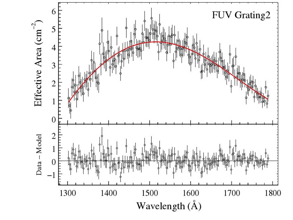
Figure 4: Effective area of the FUV2-grating as a function of wavelength

The relations between wavelength (in Angstroms) and shift (in sub-pixels) from zero order, and spectral resolutions, are shown in Table 9. Here shifts (in sub-pixels) are written as x or y to indicate whether the dispersion is along rows/columns. The effective areas plots are shown in Figure 2 to Figure 4, and the polynomial fits to the effective areas are given in Table 10.

Table 9: Dispersion solution for the different gratings of UVIT .

Order	Equation	Spectral resolution
NUV first order	$\lambda(\AA)=-5.5868x+18.1$	38 Å
FUV1 second order	$\lambda(\AA)=-2.799x+40.2$	16 Å
FUV2 second order	$\lambda(\AA)=-2.813y+33.9$	14 Å

Table 10: Polynomial fits to the effective areas (EA) for the gratings .

Parameter	Value
NUV first order	EA(cm2) = 900363.87 - 2548.8671167 $\lambda$ + 3.07510804796 $\lambda^{2}$ -
	0.0020498923174 $\lambda^{3}$ + 8.1553032340 * 10-7 $\lambda^{4}$ - 1.93655027784*10-10 $\lambda^{5}$ +
	2.5415821036*10-14 $\lambda^{6}$ - 1.42229434666*10-18 $\lambda^{7}$
FUV1 second order	EA (cm2)= -3394.60 + 8.504523 $\lambda$ - 0.0079305062 $\lambda^{2}$ + 3.2687397*10-6 $\lambda^{3}$ - 5.031413*10-10 $\lambda^{4}$
FUV2 second order	EA (cm2)= 268.14 - 1.033632 $\lambda$ + 0.0012895741 $\lambda^{2}$ - 6.5494929*10-7 $\lambda^{3}$ +1.1761863*10-10 $\lambda^{4}$

5.4 Point Spread Function (PSF) Calibration

The PSF consists of a narrow core and an extended pedestal. New results on PSF were obtained with observations of HZ 4 with short exposure frames to minimise the effect of saturation. In the photon counting mode, frames for individual exposures are analysed by the on-board hardware to communicate position of the detected photons. For shorter exposures (larger read rates) the probability of two photons occurring in one frame is less. Correction for saturation was applied as per Section 5.1.4, and it was assumed that the correction is uniform and is limited to a circle of radius 22.5 sub-pixels of the PSF. The results show that the pedestal is much more extended as compared to what was reported in Paper-1 and contains $\sim$3% more energy. The growth curves for NUV and FUV are shown in Figure 6 and Figure 7 and Table 11.

The pedestal is caused by scattering due to mechanical blocks and roughness/aberrations of the mirrors and filters and its strength is not expected to vary significantly with position on the detector. The observed variations in fractional energy of the pedestal for different filters are shown in Table 12. These data indicate that the multilayer-interference filters scatter more than the crystalline filters.

Table 13 shows that FWHM varies from $\sim$2.1 sub-pixels ($\sim$0.9^′′) to $\sim$3.4 sub-pixels ($\sim$1.4^′′) for radii $\leq$ 12^′ (fits to 2-D symmetric Gaussian give   15% larger values for FWHM). As reported in Paper-1, for larger radii ($>$12^′) the FWHM could increase up to $\sim$2^′′ due to the distortions. We note that FWHM can be adversely affected for individual exposures due to larger perturbations in the pointing or defocus due to any large variation in the temperature. Ground calibration data acquired by changing the temperature of $\pm$5 deg around the operating temperature of 20 deg found neglible changes in the telescope focus. The temperature stability achieved in space is much lesser than $\pm$ 3 deg (Sriram, 2020). From repeated observations of NGC 188, we have not found any change in the PSF with time. An analysis of the PSFs for non-saturated images shows that the sharpness of the NUV-PSF is underestimated for radii $<$7 sub-pixels; this seems to be due to a larger saturation for NUV Silica (N242W) image of HZ4 ($>$ 0.4 c/f) and the assumption that saturation is uniform for radii $<$ 22.5 sub-pixels.

Possible causes for variation in FWHM of the core are (a) defocus, due to curvature of the focal plane, tilt of the detector-plane, dispersion etc., (b) variations in errors in tracking of the drift, and (c) variations in intrinsic spatial resolution of the detector with wavelength. Images of a part of SMC were used to find FWHM, by fitting a symmetric Moffat profile, for a large number of stars within a radius of 12^′’. The results are shown in Table 13. Some systematic trends can be inferred from these data: (a) except for the filter F148W, focus for all the other FUV-filters is not optimal and the effects of curved focal plane are evident, (b) for the NUV filters the focus is optimal and the effects of curved focal plane are not significant, (c) for the FUV-filters, dispersion seems to broaden the FWHM, (d) for the NUV-filters the FWHM are better as compared to those for FUV-filters $-$ this could result from a combination of less dispersion in NUV and a better spatial resolution of the NUV-detector, and (e) filters for longer wavelengths show better FWHM $-$ this is most likely due to better spatial resolution of the detector at wavelengths closer to the cut-off wavelength resulting from lower lateral momentum/movement of the photo-electrons between the photo-cathode and MCP (see Brooks et al. 2006 for more details on this effect).

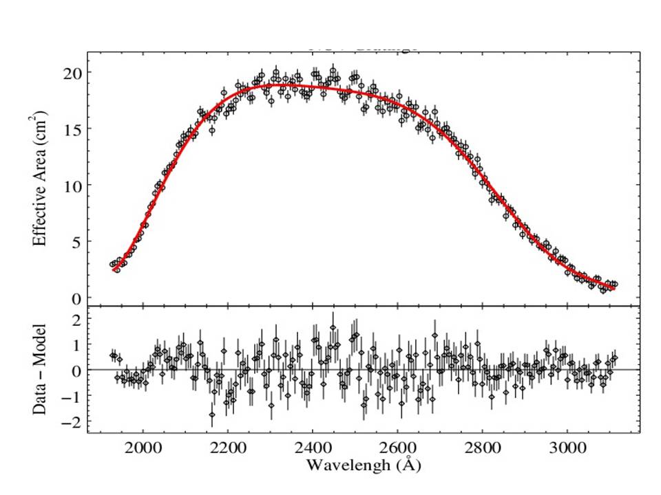
Figure 2: Effective area of the NUV-grating as a function of wavelength

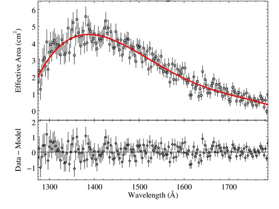
Figure 3: Effective area of the FUV1-grating as a function of wavelength

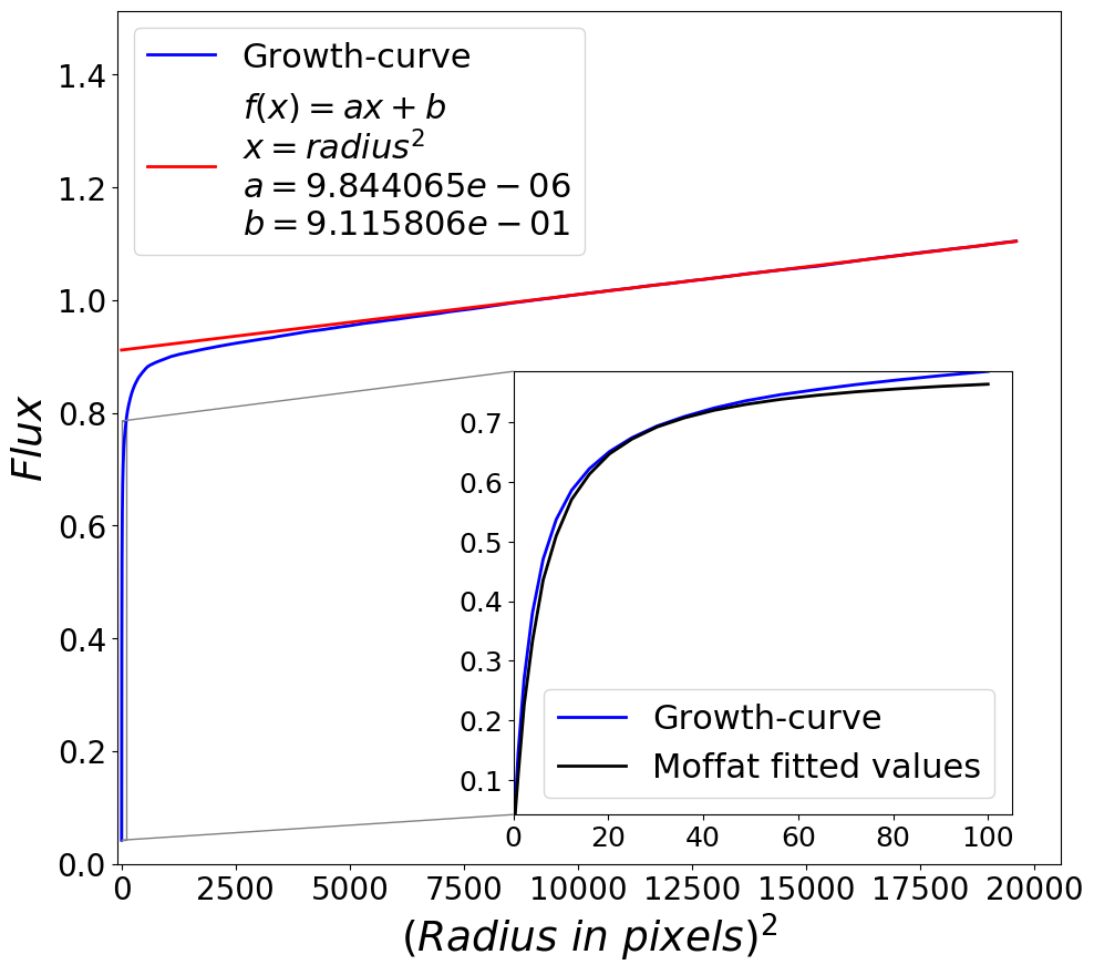
Figure 6: Growth curve (normalised by the flux obtained from 95 sub-pixels radius) for the PSF for NUV with N242W filter. The Y-axis shows total counts seen in a circle for which square of the radius (in sub-pixels) is shown on X-axis. (Small inset on top-left shows equation for the fit, and large inset at bottom-right shows magnified view of the curve.)

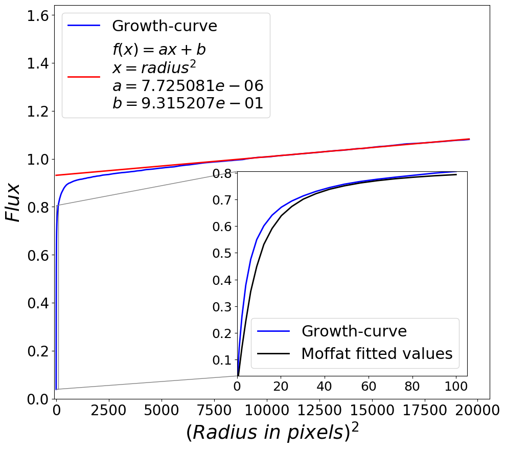
Figure 7: Growth curve (normalised by the flux obtained from 95 sub-pixels radius) for the PSF for FUV with F148W filter. The Y-axis shows total counts seen in a circle for which square of the radius (in sub-pixels) is shown on X-axis. (Small inset on top-left shows equation for the fit, and large inset at bottom-right shows magnified view of the curve.)

Table 11: Encircled energy as a function of radius in sub-pixels. This is based on analysis of the data obtained using Silica filter in NUV and CaF2 filter in FUV .

Radius	% Energy (NUV)	% Energy (FUV)
1.5	29.9	28.1
2.0	42.0	40.7
2.5	52.0	51.1
3.0	59.3	59.1
4.0	68.8	68.9
5.0	74.5	74.6
7.0	81.3	81.4
9.0	85.1	85.0
12.0	89.3	88.6
15.0	92.1	91.3
20.0	95.2	94.5
30.0	97.6	96.9
40.0	98.4	97.7
50.0	98.8	98.3
70.0	99.4	99.1
80.0	99.6	99.5
95.0	100.0	100.0

Table 12: Observed variations of energy (percentage of the total) in the pedestal. Energy in the pedestal is defined as energy between radii of 7 sub-pixels and 100 sub-pixels .

Filter	F148W	F154W	F169M	F172M	N242W	N219M	N245M	N263M	N279N
% of energy	18.6 $\pm$ 0.3	18.2 $\pm$ 0.3	18.2 $\pm$ 0.3	17.2 $\pm$ 0.3	18.7 $\pm$ 0.3	20.9 $\pm$ 0.6	19.6 $\pm$ 0.3	19.6 $\pm$ 0.3	21.8 $\pm$ 0.6

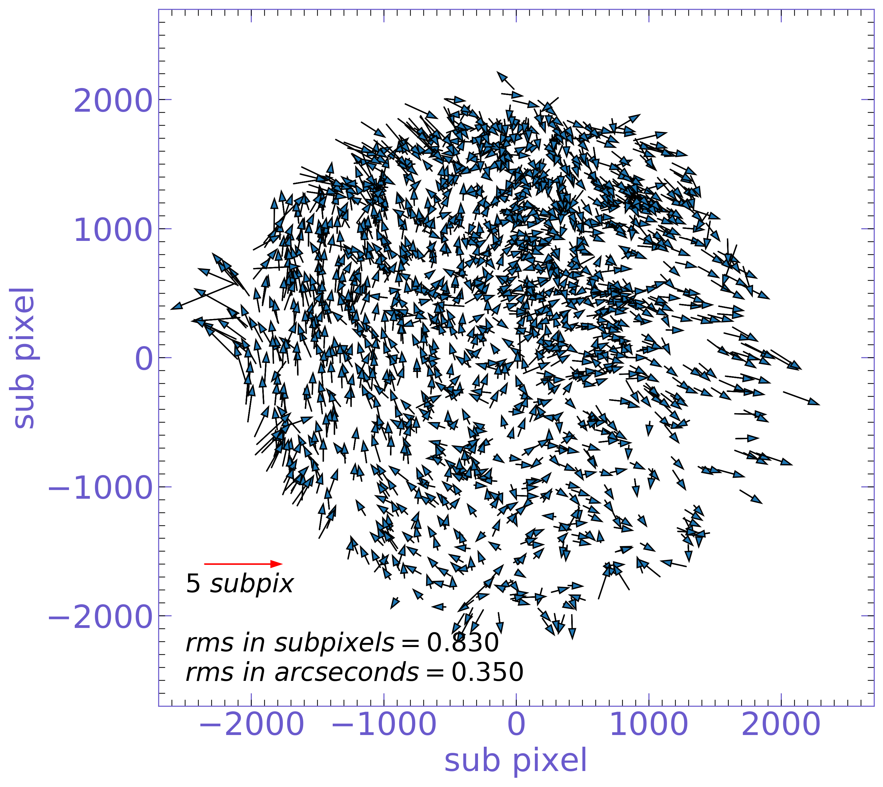
Figure 8: Relative differences in positions of the stars in the UVIT images of SMC taken with FUV-F154W and NUV-N263M are shown as vectors, where tail of the vector corresponds to position in the NUV field. Positions and errors are shown in sub-pixels. For radii $<$ 1900 sub-pixels, any source giving an error $>$ 2 sub-pixels is either a close double or is at a radius $>$ 1900 sub-pixels in the FUV detector

5.5 Astrometric Calibration

Positions measured by the detectors show deviations from linearity, i.e. the detectors show distortion. The distortions were calibrated on the ground and a part of these data were used to correct the measured positions for the results reported in Paper-1. Now, all the data on calibration have been used to correct the measured positions. The resulting corrections differ significantly for NUV near edges in the first quadrant. To get an estimate of the distortion in the final images, positions of stars in the NUV-images of SMC with filter N263M were compared with the positions in the FUV image with filter F154W, after due corrections for the relative plate scale and shift & rotation between the two images. The differences are shown in Figure 8. It is seen that the new results are significantly better than those reported in Paper-1 for x $>$ 1800 sub-pixels in the first quadrant. Averaged over the full field, rms of the deviations is $<$ 0.4^′′. while it is 0.3^′′ within a diameter of 24^′. As the optics and the detectors for FUV and NUV are independent, these differences can be taken as upper bound for leftover distortion in the individual images.

Table 13: Observed variations (in sub-pixels) of the FWHM with positions across the detector. For FUV filters, the first number is for stars at radii $<$ 7.5 arcmin, and the second number is for stars at radii $>$ 7.5 armimn and $<$ 12 arcmin, while for NUV filters the number is for all the stars within a radius of 12 arcmin and no significant variation in FWHM with radius was seen .

Filter	F148W	F154W	F169M	F172M	N242W	N219M	N245M	N263M	N279N
FWHM	3.06,3.11	3.37,3.11	3.10,2.66	3.15,2.78	2.63	2.75	2.59	2.10	2.19

6 Conclusion

Based on additional data, results on the calibration for UVIT have been revisited. Results on all calibration except flat field show only small differences as compared to the results reported in Paper-1. Details on the new calibration that are needed for the users of UVIT data along with the updated CALDB are also available at https://uvit.iiap.res.in/. We summarize here the findings of the calibration

1. Photometric calibration: (a)as compared to estimates from the ground calibration, reduction in sensitivity ( or average effective area) for all the filters except N219M lie in range of 11% to 22%, while the filter N219M shows a reduction of $\sim$46%. These differences are most likely related to inaccuracies in the ground calibration which were only meant to assure that the sensitivities in different bands were not less than 50% of the designed value. (b) The peak to peak variation in sensitivity with position within a diameter of 24^′ is $<$ 20% for all the filters except N219N for which it is $\sim$35% and (c) new zero point magnitudes are estimated with reference to the white dwarf HZ 4.

2. Repeated observations of 2 stars in NGC 188 over 3 years in the orbit show no reduction in the sensitivity of the FUV and NUV channels.

3. Spectroscopic calibration give a peak effective area of $\sim$18.5 sq cm and a resolution of 38 Å for the NUV grating, and a peak effective area of $\sim$4.5 sq cm and a resolution of $\sim$15 Å for the FUV gratings,

4. The PSF shows a FWHM 1.4^′′ or better within a diameter of 24^′ for FUV as well as NUV.

5. Astrometric calibration in orbit shows that the uncorrected distortion is $<$ 0.3^′′ rms within a diameter of 24^′.

References

- Agrawal (2006) Agrawal, P. C. 2006, Advances in Space Research, 38, 2989
- Brooks et al. (2006) Brooks, R., Ingle, M., Milnes, J., Howorth, J., & Hutchings, J. 2006, in Proc. SPIE, Vol. 6294, Society of Photo-Optical Instrumentation Engineers (SPIE) Conference Series, 62940W
- Dewangan (2019) Dewangan, G. 2019, Private communication
- Noter et al. (1993) Noter, Y., Nahor, G., Lifshitz, Y., Saar, N., & Braun, O. 1993, Society of Photo-Optical Instrumentation Engineers (SPIE) Conference Series, Vol. 1971, Contamination control approach for the TAUVEX UV astronomical telescope, ed. M. Oron, I. Shladov, & Y. Weissman, 276–287
- Poole et al. (2008) Poole, T. S., Breeveld, A. A., Page, M. J., et al. 2008, MNRAS, 383, 627
- Postma & Leahy (2017) Postma, J. E., & Leahy, D. 2017, PASP, 129, 115002
- Sriram (2020) Sriram, S. e. a. 2020, In preparation
- Tandon et al. (2017a) Tandon, S. N., Subramaniam, A., Girish, V., et al. 2017a, AJ, 154, 128
- Tandon et al. (2017b) Tandon, S. N., Hutchings, J. B., Ghosh, S. K., et al. 2017b, Journal of Astrophysics and Astronomy, 38, 28