Second law of thermodynamics at stopping times

Abstract

Events in mesoscopic systems often take place at first-passage times, as is for instance the case for a colloidal particle that escapes a metastable state. An interesting question is how much work an external agent has done on a particle when it escapes a metastable state. We develop a thermodynamic theory for processes in mesoscopic systems that terminate at stopping times, which generalize first-passage times. This theory implies a thermodynamic bound, reminiscent of the second law of thermodynamics, for the work exerted by an external protocol on a mesoscopic system at a stopping time. As an illustration, we use this law to bound the work required to stretch a polymer to a certain length or to let a particle escape from a metastable state.

Introduction.

How much work do we need to do on a mesoscopic system in order to let a certain event of interest happen? For example, how much work do we require to stretch a polymer to a certain length or to let a colloidal particle escape from a metastable state, as illustrated in Fig. 1? The latter is Kramers’ escape problem kramers1940brownian ; hanggi1986escape , which models, inter alia, biochemical reactions and the escape of particles from bounded domains hanggi1990reaction ; Bressloff2013 ; Bressloff2014 . Although it is well understood how long it takes for a particle to escape a metastable state, see e.g. Refs. Gardiner ; Sidney2001 ; Grebenkov2014 , little is known about the average work done on a particle when it escapes a metastable state.

Stochastic thermodynamics is a thermodynamic theory for mesoscopic systems jarzynski1997nonequilibrium ; jarzynski1997equilibrium ; crooks1998nonequilibrium ; crooks1999nonequilibrium ; maes2003origin ; jarzynski2011equalities ; Sek2010 ; seifert2012stochastic ; van2015ensemble and provides experimental testable predictions for their fluctuating properties Ciliberto ; Gladrow . An important result in stochastic thermodynamics is the second-law-like bound jarzynski1997nonequilibrium ; jarzynski1997equilibrium

$$\langle W(t)\rangle\geq f\left(\lambda_{\rm f}\right)-f\left(\lambda_{\rm i}\right)$$ (1)

on the average work $\langle W(t)\rangle$ done on a system in a fixed time interval $[0,t]$ as a function of the free energy difference between the final and initial states, characterized by parameters $\lambda_{\rm f}=\lambda(t)$ and $\lambda_{\rm i}=\lambda(0)$, respectively. In what follows we denote random variables with uppercase letters and deterministic variables with lowercase letters. Averages $\langle\cdot\rangle$ are over repeated realizations of the process.

Unfortunately, the bound given by Eq. (1) does not provide much insights on the average work $\langle W(T)\rangle=\langle\int^{T}_{0}W(t){\rm d}t\rangle$ done on the system at an event of interest. Indeed, the time $T$ when an event — such as the escape of a particle from a metastable state — takes place will be different for each realization of the process, and therefore the second law given by Eq. (1) does not apply.

In this paper we derive a fundamental bound on the average work an external agent has done on a system at times $T$ when an event happens, which we call a stopping time. This law reads

$$\langle W(T)\rangle\geq\langle f(\lambda(T))\rangle-f(\lambda_{\rm i})+\beta^{-1}\langle\pi(T)\rangle,$$ (2)

where $\langle\pi(T)\rangle$ is a correction term that accounts for the fact that the process is in general out of equilibrium at the stopping time $T$, and whose precise form we will specify later. We call this law the second law of thermodynamics at stopping times. To derive the second law given by Eq. (2), we develop a thermodynamic theory for events in nonstationary processes that take place at random times and which relies on martingale theory Chetrite2011 ; neri2017statistics ; neri2019integral .

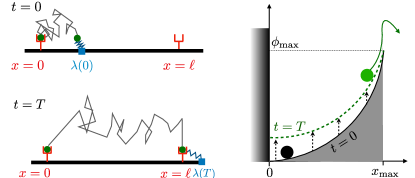
Figure 1: Stretching a polymer to a certain length $\ell$ (Panel (a)) or letting a particle escape from a metastable state (Panel(b)). Panel (a): An external agent (blue square) is connected with a spring (blue zigzag line) to one of the end points (green circles) of a polymer (grey zigzag line) and stretches the polymer until it reaches a length $\ell$, after which the polymer end point is attached to an anchor point (red object). Panel (b): a colloidal particle (full circle) escapes from a metastable state under the influence of an external protocol $\lambda(t)$ that changes the shape of the potential $\phi(x;\lambda)$.

System setup.

We consider a mesoscopic system composed of slow and fast degrees of freedom. The fast, internal degrees of freedom are hidden, whereas the slow degrees of freedom are observed and take values in $\mathcal{X}$.

We assume that the system interacts weakly with an environment that is in a state of thermal equilibrium at temperature $1/\beta$. For a given value of the external parameter $\lambda$, the system admits an equilibrium state

$$p_{\rm eq}(x;\lambda)=e^{-\beta[\phi(x;\lambda))-f(\lambda)]},\quad x\in\mathcal{X},$$ (3)

where $\phi$ is the free energy for a fixed value $x$ of the slow degrees of freedom and where $f$ is the free energy of the total system. The free energy

$$\phi(x;\lambda)=u(x;\lambda)-s_{\rm int}(x;\lambda)/\beta$$ (4)

is the sum of the internal energy $u$ and the entropy $s_{\rm int}$ associated with the internal degrees of freedom.

We assume that the system is in thermal equilibrium with its environment at $t\leq 0$, and at time $t=0$ the system engages with an external protocol that drives it out of equilibrium. The protocol consists in a change of the external parameter $\lambda(t)$, such that, $\lambda(t)=\lambda_{\rm i}$ for $t\leq 0$ and $\lambda(t)=\lambda_{\rm f}$ for $t>\tau$.

We assume that the internal degrees of freedom equilibrate on time scales that are much shorter than those over which $\lambda(t)$ varies (the protocol is quasi-static with respect to the internal degrees of freedom).

We aim to quantify the work done on the system at the moment when a certain event happens (for example the escape of a particle from a metastable state). The time when an event happens is modelled with a stopping time $T$. We say that a random time $T\in[0,\infty)\cup\left\{+\infty\right\}$ is a stopping time if it is a deterministic function defined on the set of trajectories $X^{+\infty}_{0}=\left\{X(t)\right\}_{t\in\mathbb{R}^{+}}$ that obeys causality; in other words, the value of the stopping time $T$ is independent of the outcomes of the process $X$ after the stopping time. If the event does not occur, then $T=+\infty$ Williams1991 ; Protter ; Liptser2013 .

The probability measure $\mathbb{P}$ describes the probability of events in the forward dynamics (i.e, with the protocol $\lambda(t)$ and initial distribution $p_{\rm eq}$) and we denote expectation values with respect to this measure by $\langle\cdot\rangle_{\mathbb{P}}=\langle\cdot\rangle$.

Time-reversibility and martingales.

An important feature of mesoscopic systems is that they are time-reversible. Time-reversibility is defined relative to the backward dynamics that we define as follows seifert2012stochastic : the state is in the equilibrium state $p_{\rm eq}(x;\lambda_{\rm f})$ for all times $t<0$ and is subsequently driven out of equilibrium by the protocol $\tilde{\lambda}(t)=\lambda(\tau-t)$.

The dynamics of a mesoscopic system is time reversible if there exists a process $S(t)$, defined on the set of trajectories $X^{t}_{0}$, such that

$$\langle A(t)\rangle_{\mathbb{P}}=\langle A(t)e^{S(t)}\rangle_{\tilde{\mathbb{P}}\circ\Theta}$$ (5)

holds for any observable $A(t)$ that is a function of $X^{t}_{0}$, where the measure $\tilde{\mathbb{P}}$ describes the statistics of the process in the backward dynamics. The map $\Theta$ is the time-reversal map that mirrors trajectories relative to the time point $\tau/2$, such that $\Theta\left[X^{+\infty}_{-\infty}\right]=\left\{X(\tau-t)\right\}_{t\in\mathbb{R}}$. In other words, the expectation value of an observable in the forward dynamics can be expressed in terms of the expectation value of the same observable in the backward dynamics, as long as it is properly reweighted with the process $e^{S(t)}$.

The Eq. (5) implies that

$$e^{-S(t)}=\Big{\langle}\frac{\tilde{p}\left[\Theta(X^{+\infty}_{-\infty})\right]}{p\left[X^{+\infty}_{-\infty}\right]}\Big{|}X^{t}_{0}\Big{\rangle}_{\mathbb{P}}$$ (6)

where $\tilde{p}\left[\Theta(X^{+\infty}_{-\infty})\right]/p\left[X^{+\infty}_{-\infty}\right]$ is the Radon-Nikodym derivative between the two measures $\tilde{\mathbb{P}}\circ\Theta$ and $\mathbb{P}$ Liptser2013 , or loosely said, the ratio between the two associated probability densities, and where $\Big{\langle}\cdot\Big{|}X^{t}_{0}\Big{\rangle}_{\mathbb{P}}$ is a conditional expectation given $X^{t}_{0}$. The quantity $e^{-S(t)}$ exists as long as the two measures $\tilde{\mathbb{P}}\circ\Theta$ and $\mathbb{P}$ are mutually absolutely continuous, which holds since the interval $[0,\tau]$ is finite and the microscopic laws of physics are time reversible.

Equation (6) implies that $e^{-S(t)}$ is a regular martingale. Martingales are stochastic processes that model a gambler’s fortune in a fair game of chance snell1982gambling or stock prices in efficient capital markets leroy1989efficient . We say that a stochastic process $M(t)$ is a martingale relative to another stochastic process $X(t)$ if: (i) the process $M(t)$ is a real-valued function on the set of trajectories $X^{t}_{0}$; (ii) the process $M(t)$ is integrable, i.e., $\langle|M(t)|\rangle<\infty$; (iii) the process $M(t)$ has no drift, i.e., with probability one $\langle M(t)|X^{s}_{0}\rangle=M(s)$ for all $s<t$ Doob1953 ; Doob1971 ; Williams1991 ; Liptser2013 .

An important class of martingales are regular martingales Doob1940 ; Liptser2013 . Let $Y$ be an integrable, real-valued random variable that is a function of the trajectory $X^{+\infty}_{-\infty}$. Then the process

$$M(t)=\langle Y|X^{t}_{0}\rangle,\quad t\in I,$$ (7)

is a regular martingale, where $\langle\cdot|\cdot\rangle$ denotes a conditional expectation. The martingality of $\langle Y|X^{t}_{0}\rangle$ is a direct consequence of the tower property of conditional expectations, viz., $\langle\langle Y|X^{t}_{0}\rangle|X^{s}_{0}\rangle=\langle Y|X^{s}_{0}\rangle$ for all $s\leq t$.

Doob’s optional stopping theorem and a second-law like relation at stopping times.

A useful property of regular martingales is Doob’s optional stopping theorem, which states that for a regular martingale $M(t)$ and for a stopping time $T$ it holds that $\langle M(T)\rangle=\langle M(0)\rangle$, see Theorems 3.2 in Ref. Liptser2013 . Doob’s optional stopping theorem implies that a gambler cannot make fortune by quitting a fair game of chance at an intelligently chosen moment $T$.

Applying Doob’s optional stopping theorem to $e^{-S(t)}$, we obtain the following integral fluctuation relation at stopping times,

$$\langle e^{-S(T)}\rangle=\langle e^{-S(0)}\rangle=1.$$ (8)

Using Eq. (8) and Jensen’s inequality $\langle e^{-S(T)}\rangle\geq e^{-\langle S(T)\rangle}$, we obtain

$$\langle S(T)\rangle\geq 0,$$ (9)

which is a second-law-like inequality.

Principle of local detailed balance.

The Eq. (9) is similar to a second law of thermodynamics, but misses a connection with the work done on the system. We use the principle of local detailed balance crooks1998nonequilibrium ; crooks1999nonequilibrium ; maes2003origin ; jarzynski2011equalities ; Sek2010 ; seifert2012stochastic ; van2015ensemble to link $S(t)$ with the work $W(t)$. We say that a process obeys local detailed balance if $S(t)$ is the total entropy production, i.e.,

$$S(t) = -\beta Q(t)+s_{\rm int}(X(t);\lambda(t))-s_{\rm int}(X(0);\lambda_{\rm i})$$ (10)

$$-\log\tilde{p}_{\tau-t}(X(t))+\log p_{\rm eq}(X(0);\lambda_{\rm i}).$$

The first term on the right-hand side is the dissipated heat divided by the temperature and equals the change in the environment entropy. The second term is the change in the internal entropy (associated with the internal degrees of freedom) and the last term is the change in system entropy (associated with the observed degrees of freedom). The distribution $\tilde{p}_{\tau-t}(x)$ is the probability distribution of the time-reversed process at time $\tau-t$ (with external parameter $\tilde{\lambda}(\tau-t)$). If $t\geq\tau$, then $\tilde{p}_{\tau-t}(x)=p_{\rm eq}(x;\lambda_{\rm f})$, whereas if $t<\tau$ then $\tilde{p}_{\tau-t}(x)$ is obtained by evolving the state $p_{\rm eq}(x;\lambda_{\rm f})$ over a time interval $s\in[0,\tau-t]$ using the time-reversed protocol $\tilde{\lambda}(s)=\lambda(\tau-s)$. Using the first law of thermodynamics

$$Q(t)+W(t)=u(X(t);\lambda(t))-u(X(0);\lambda_{\rm i})$$ (11)

and the Boltzmann distribution, given by Eq. (3), we obtain the expression (see Supplemental Material Supplement )

$$S(t)=\beta[W(t)-f(\lambda(t))+f(\lambda_{\rm i})]-\pi(t)$$ (12)

where

$$\pi(t)=\log\frac{\tilde{p}_{\tau-t}(X(t))}{p_{\rm eq}(X(t);\lambda(t))}.$$ (13)

Second law of thermodynamics at stopping times.

The Eq. (9) together with Eq. (12) implies the second law of thermodynamics at stopping times Eq. (2) where

$$\langle f(T)\rangle=\int^{\infty}_{0}{\rm d}t\>p_{T}(t)f(t)$$ (14)

and

$$\langle\pi(T)\rangle = \int^{\infty}_{0}{\rm d}t\>\int_{\mathcal{X}}{\rm d}x\>p_{T,X(T)}(t,x)\log\frac{\tilde{p}_{\tau-t}(x)}{p_{\rm eq}\left(x;\lambda(t)\right)},$$

is a correction term that accounts for the fact that at the stopping time the state may be far from thermal equilibrium. The distribution $p_{T,X(T)}(t,x)$ is the joint probability distribution of $T$ and $X(T)$ in the forward dynamics and $p_{T}(t)$ is the probability distribution of the stopping time $T$.

The second law of thermodynamics at stopping times, given by Eq. (2), is the main result of this Letter. It bounds the average work that a mesoscopic system requires to execute a certain task, which is completed at a stopping time $T$. It is reminiscent of second-law-like relations derived in Ref. neri2019integral . However, the paper neri2019integral deals with stationary systems, whereas the Eq. (2) holds for nonstationary systems.

The Eq. (8) together with Eq. (12) implies

$$\langle e^{-\beta[W(T)-f(\lambda(T))+f(\lambda_{\rm i})]+\pi(T)}\rangle=1,$$ (16)

which is a Jarzynski-like relation jarzynski1997nonequilibrium ; jarzynski1997equilibrium that holds at stopping times.

Limiting cases.

In experiments or numerical simulations it can be a daunting task to evaluate the quantity $\pi(t)$. Fortunately, it turns out that $\pi(T)=0$ in several limiting cases. In these cases we obtain the appealing bound

$$\langle W(T)\rangle\geq\langle f(\lambda(T))\rangle-f(\lambda_{\rm i}).$$ (17)

Examples of limiting cases for which Eq. (17) holds are when: (i) the stopping time $T$ is larger than $\tau$. Indeed, if $t>\tau$ then $\tilde{p}_{\tau-t}(x)=p_{\rm eq}(x;\lambda_{\rm f})$ and $\pi(t)=0$; (ii) the driving $\lambda(t)$ is quasi-static. In this case, $\tilde{p}_{\tau-t}(x)=p_{\rm eq}(x;\lambda(t))$ for all $t$, such that $\pi(t)=0$; (iii) the protocol is quenched (i.e., $\lambda(t)=\lambda_{\rm f}$ for $t>0$) and the probability that $T=0$ is equal to zero (see supplemental material for a proof Supplement ).

Interestingly, if the probability that $T=0$ is equal to zero, then $\pi(T)=0$ for a protocol $\lambda(t)$ that changes slowly (quasi-static) and also for a protocol $\lambda(t)$ that changes quickly (quenched). Hence, we may expect that $\pi(T)\approx 0$ holds for intermediate driving speeds too. This can be verified through the Jarzynski relation at stopping times Eq. (16), which simplifies into

$$\langle e^{-\beta[W(T)-f(\lambda(T))+f(\lambda_{\rm i})]}\rangle=1$$ (18)

when $\pi(T)=0$.

In the next paragraphs, we use the second-law relations at stopping times Eqs. (2) and (17) to bound the work required to stretch a polymer or to let a particle escape.

Stretching a polymer.

We ask how much work is required to stretch a polymer to a certain length $\ell$, as is illustrated in Fig. 1(a), and we apply the bound Eq. (2) to this example. We consider a setup where one end of the polymer is anchored at position $x=0$ to a substrate, whereas the other end is fluctuating and described by a stochastic process $X(t)\in\mathbb{R}$. The dangling end of the polymer is connected with a spring to an external agent, say a molecular motor, centered at $\lambda(t)$. At $t=0$, the molecular motor starts to move and stretches the polymer until it reaches a length $\ell$, at which point the motor stops moving and the second end point of the polymer is anchored to the substrate.

We assume that the dynamics of $X(t)$ is well described by a one-dimensional overdamped Langevin equation

$$\frac{{\rm d}X}{{\rm d}t}=-\mu\>\partial_{x}\phi(X;\lambda(t))+\sqrt{2d}\>\xi(t),\quad t\geq 0,$$ (19)

where $\mu$ is the mobility coefficient, $d=\mu/\beta$ is the diffusion coefficient, $\xi(t)$ is a Gaussian white noise with $\langle\xi(t)\rangle=0$ and $\langle\xi(t)\xi(t^{\prime})\rangle=\delta(t-t^{\prime})$, and where

$$\phi(x;\lambda(t))=\frac{\kappa_{\rm p}}{2}\>x^{2}+\frac{\kappa_{\rm m}}{2}\left(x-\lambda(t)\right)^{2}$$ (20)

is the sum of the free energy $\kappa_{\rm p}x^{2}/2$, of a polymer with one of its end points anchored to the substrate at $x=0$, and the free energy $\kappa_{\rm m}\left(x-\lambda(t)\right)^{2}/2$, of the spring that connects the dangling end point of the polymer to the molecular motor located at $\lambda(t)$. Furthermore, we assume that at the initial time $t=0$ this polymer system is in thermal equilibrium with its surroundings and that the dynamics of the motor is given by

$$\lambda(t)=\lambda_{\rm i}+(\lambda_{\rm f}-\lambda_{\rm i})\frac{1-e^{-t/\tau_{\rm prot}}}{1-e^{-\tau/\tau_{\rm prot}}},\quad t\in[0,\tau],$$ (21)

where $\tau_{\rm prot}>0$ characterises the speed of the protocol. The quantity $\tau_{\rm rel}=1/(\mu(\kappa_{\rm m}+\kappa_{\rm p}))$ is the polymer relaxation time. If $\tau_{\rm prot}\ll\tau_{\rm rel}$, then the molecular motor quenches the polymer, whereas if $\tau_{\rm prot}\gg\tau_{\rm rel}$, then the motor stretches the polymer in a quasi-static manner.

The work the motor performs on the polymer is Sek1998

$$W(t)=\int^{t}_{0}{\rm d}s\>\partial_{\lambda}\phi(X(s);\lambda)\>\dot{\lambda}_{s}.$$ (22)

Fig. 2(a) presents the average work $\langle W(T)\rangle$ for $T={\rm inf}\left\{t\in[0,\tau]:|X(t)|\geq\ell\right\}$, in other words, the motor stops as soon as the polymer’s length exceeds $\ell$, and we compare it with the second-law-like bound Eq. (2) (see Supplemental Material for details Supplement ). Interestingly, we observe that for all values of $\tau_{\rm prot}$ the term $\langle\pi(T)\rangle\approx 0$ and that $\langle W(T)\rangle\geq\langle f(\lambda(T))\rangle-f(\lambda_{i})$, consistent with the bound Eq. (17). As discussed in the previous paragraph, this can be understood from the fact that if $\mathbb{P}(T=0)$, then $\pi(T)=0$ in both the quasi-static and quenched limits.

For $\tau_{\rm prot}$ large enough, $\langle W(T)\rangle\rightarrow 0$. Indeed, if $\tau_{\rm prot}>\tau_{\rm fp}$ — where $\tau_{\rm fp}=\frac{\sqrt{\pi}\ell^{2}}{4d}\frac{e^{\alpha}}{\alpha^{3/2}}$ is the mean-first passage time $\langle T\rangle$ when $\lambda_{\rm f}=\lambda_{\rm i}$, with $\alpha=\beta\frac{(\kappa_{\rm p}+\kappa_{\rm m})\ell^{2}}{2}$ Grebenkov2014 — then the polymer extends spontaneously due to thermal fluctuations and $\langle W(T)\rangle\approx 0$.

Escape problem.

We determine how much work is required to let a colloidal particle escape a metastable state, as is illustrated in Fig. 1(b). We consider a particle described by the overdamped Langevin Eq. (19) with potential

$$\phi(x;\lambda)=(\phi_{\rm max}-\lambda)\frac{x^{2}}{x^{2}_{\rm max}}+\lambda,\quad x\in[0,x_{\rm max}],$$ (23)

and reflecting boundary condition at $x=0$. Initially, the particle is trapped in the metastable state with Boltzmann distribution, given by Eq. (3), and with $\lambda=\lambda_{\rm i}=0$.

We compute the average work done on the particle, given by Eq. (22), at the escape time $T={\rm inf}\left\{t\geq 0:X(t)\geq x_{\rm max}\right\}$. In the absence of a driving force, the particle escapes in a time $\langle T\rangle=\tau_{\rm fp}\sim e^{\beta\phi_{\rm max}}$, which is very large when $\beta\phi_{\rm max}\gg 1$. Therefore, we facilitate the particle’s escape with a kick that deforms the potential landscape as $\lambda(t)=\lambda_{\rm k}e^{-t/\tau_{\rm prot}}$ for $t\geq 0$. Interestingly, Fig. 2(b) shows that the bound Eq. (17) is satisfied, which indicates that again $\pi(T)\approx 0$. This is confirmed with an evaluation of the Jazynski Eq. (18) at stopping times.

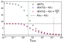
Figure 2: Simulation results for stretching a polymer (Panel (a)) and the escape problem (Panel (b)). Panel (a): model parameters are $\ell=2.2$, $\mu=0.1$, $\beta=\kappa_{\rm p}=1$, $\kappa_{\rm m}=2$, $\lambda_{\rm i}=0.2$, $\lambda_{\rm f}=5$, and $\tau=1e+6$. The relaxation time $\tau_{\rm rel}=10/3$ and the mean first-passage time $\tau_{\rm fp}\approx 1560$ are denoted by the vertical dotted lines. The black solid line equals zero and is a guide to the eye. Panel (b): model parameters are $\mu=0.1$, $\beta=x_{\rm max}=1$, $\phi_{\rm max}=10$, and $\tau_{\rm prot}=4$. Markers are averages over $1e+4$ realizations of the process.

Discussion.

In mesoscopic systems, physical events often happen at random times, such as, the escape of a colloidal particle from a metastable state Sidney2001 ; Bressloff2013 ; Bressloff2014 ; Grebenkov2014 . We have derived the second law of thermodynamics at stopping times Eq. (2), which bounds the average amount of work that has been done on a system at a stopping time or first-passage time $T$ as a result of a change in the free-energy landscape. This second law applies to arbitrary systems that obey local detailed balance and arbitrary stopping times.

If $\langle\pi(T)\rangle\approx 0$, then the second law Eq. (2) simplifies into Eq. (17). Interestingly, we have shown that Eq. (17) holds in the quasi-static limit and for quenched protocols when $T>0$ with probability one. Additionally, using numerical simulations we find that in our examples Eq. (17) holds at intermediate driving speeds of the protocol, and I believe this will be in general the case (as long as $T>0$ with probability one).

If $\langle\pi(T)\rangle<\beta[f(\lambda_{\rm i})-\langle f(\lambda(T))\rangle]$, then the system can perform work on its environment. For instance, we can stop the process as soon as $W(t)>\epsilon$, with $\epsilon$ a small positive number (see Supplemental Material for an example). Work extraction by stopping a process at an intelligently chosen moment is closely related to the construction of Maxwell demons, which are smart devices that change the protocol of a system at a cleverly chosen moment Par . However, in the thermodynamics at stopping times we do not consider what happens after the stopping time (e.g. in the escape problem we are not interested in the events that happen after the particle has escaped the potential).

The present Letter demonstrates how for nonstationary processes thermodynamic relations at stopping times can be derived using the martingale $e^{-S(t)}$ given by Eq. (6); so far, thermodynamic properties of stochastic processes at first-passage times have mainly been studied in the context of stationary processes roldan2015 ; neri2017statistics ; garrahan ; Gingrich ; quantum ; neri2019integral . It would be interesting to use the martingality of $e^{-S(t)}$ to derive bounds on, e.g., extreme values of $Q(t)$ Singy or mean first-passage times roldan2015 in nonstationary processes.

See pages 1 of SuppMat2.pdf See pages 2 of SuppMat2.pdf See pages 3 of SuppMat2.pdf See pages 4 of SuppMat2.pdf See pages 5 of SuppMat2.pdf See pages 6 of SuppMat2.pdf See pages 7 of SuppMat2.pdf See pages 8 of SuppMat2.pdf See pages 9 of SuppMat2.pdf