Reconstructing the radial velocity profile of cosmic voids with kinematic Sunyaev-Zeldovich Effect

Abstract

We develop an estimator to extract the mean radial velocity profile of cosmic voids via the kinematic Sunyaev-Zeldovich effect of pairs of galaxies surrounding them. The estimator is tested with simulated pure kSZ map and void catalogue data from the same simulation. The results show that the recovered signal could be attenuated by low angular resolution of the map or large aperture photometry filter radius size, but the mean radial velocity profile can be fully recovered with our estimator. By applying the estimator to the Planck 2D-ILC CMB map, with galaxy and void catalogues from BOSS DR12, we find that the estimated void velocity profile is $3.31\sigma$ apart from null detection for for voids with continuously rising density profiles asymptoting to the mean density; and $1.75\sigma$ for voids with positive density contrast shell surrounded. By fitting the reconstructed data to the theoretical profile, we find the reduced $\chi^{2}$ to be $1.19$ and $0.62$ for the two types of void, respectively, indicating a good fit of the model to the data. We then forecast the detectability of the radial velocity profile of cosmic voids with future CMB surveys, including SPT-3G, AdvACT, and Simons Observatory. We find that the contamination effect from CMB residuals is negligible with survey area over $2,000\deg^{2}$, especially with aperture photometry size less than $1\,{\rm arcmin}$. But the effect from instrumental noise is non-negligible. For future SPT-3G, AdvACT and Simons Observatory, the detection is potentially achievable from $3\sigma$ to $10\sigma$ C.L., depending on specific instrumental parameters. This opens a new window of probing dynamics of the cosmic structures from the kinematic Sunyaev-Zeldovich effect.

I Introduction

The kinematic Sunyaev-Zeldovich effect (hereafter, kSZ effect) is the secondary CMB anisotropy effect due to its scattering off moving electrons in the Universe Sunyaev and Zeldovich (1972, 1980)

$$\frac{\Delta T}{T}=-\frac{\sigma_{\rm T}}{c}\int{\rm d}l\,n_{\rm e}\,(\mathbf{v}\cdot\hat{\mathbf{n}}),$$ (1)

in which, $\sigma_{\rm T}$ is the Thomson cross-section, $n_{\rm e}$ is the electron density and $\mathbf{v}$ is the peculiar velocity of electrons relative to the CMB. The kSZ signal was first detected by Ref. Hand et al. (2012) via pairwise kSZ estimator proposed in Refs. Ferreira et al. (1999); Juszkiewicz et al. (2000), using the CMB data from Atacama Cosmology Telescope (ACT Swetz et al. (2011)) and the galaxy catalogue from the Sloan Digital Sky Survey III DR9 Ahn et al. (2012). Since then, there has been a number of works to detect the kSZ effect at various levels by cross-correlating CMB data with other large-scale structure tracers. These include the pairwise kSZ estimates with South Pole Telescope (SPT) data and Dark Energy Survey (DES) cross-correlation Soergel et al. (2016), Atacama Cosmology Telescope (ACT) data and SDSS/DR11 cross-correlation De Bernardis et al. (2017), Planck and SDSS/DR12 cross-correlation Sugiyama et al. (2018); Li et al. (2018); kSZ cross-correlation with reconstructed peculiar velocity field Planck Collaboration et al. (2016a); Hernández-Monteagudo et al. (2015); the squared kSZ field cross-correlation with projected density field from WISE infra-red survey Hill et al. (2016); Ferraro et al. (2016); the kSZ dispersion measurement with Planck data and X-rays selected clusters Planck Collaboration et al. (2017). More recently, Ref. Baxter et al. (2019) detected the rotational kSZ effect with Planck map and six rotational cluster samples from SDSS/DR10.

Despite the rapid progress of kSZ detection in this field, little work has been done to investigate the behaviour of cosmic void, which is believed to dominate the cosmic volume on large scales. The cosmic voids refers to the large underdensity region of matter distribution in the Universe. During the cosmic evolution, matters are accredited into the galaxies and clusters due to the gravitational attraction, therefore leaving more and more empty and underdense region in the Universe. The properties of the voids, such as the abundance or the spatial distribution, are related to the initial conditions and the universe evolution history Sheth and van de Weygaert (2004); Martino and Sheth (2009). In the meanwhile, the voids properties also depend on the nature of the gravity Clampitt et al. (2013); Cai et al. (2015). With $N$-body simulations, one can explore the gravitational physics of the void formation Dubinski et al. (1993); Sheth et al. (2001), the statistical properties of the void distribution Martino and Sheth (2009); Tramonte et al. (2017), and the density and velocity profiles Hamaus et al. (2014); Cautun et al. (2016); Demchenko et al. (2016); Massara and Sheth (2018).

Recently, several cosmic void catalogues have been compiled from galaxy redshift survey data Pan et al. (2012); Sutter et al. (2012); Nadathur and Hotchkiss (2014); Mao et al. (2017). Studies with such cosmic void catalogue and numerical simulations suggest that it is possible to classify voids into two different types according to their surrounding density profiles. The “S-type” voids are surrounded by a shell of positive density contrast $\delta$ which compensates the mass deficit within the void. The “R-type” voids instead have continuously rising density profiles asymptoting to the mean density Ceccarelli et al. (2013). The different gravitational lensing effects on the CMB of these types of voids were recently detected Raghunathan et al. (2019). The different density environment leads to different velocity fields around cosmic voids. Using mock galaxy and voids catalogue, Ceccarelli et al. (2013) showed that S-type voids have infall velocities outside of the overdense shell whereas inside the overdense shell the voids are expanding. In contrast, R-type voids only expand and experience no contraction around void radius. Void velocity and density profiles can be measured observationally via the RSD effect in the void-galaxy cross-correlation Paz et al. (2013); Cai et al. (2016); Pisani et al. (2019); Nadathur et al. (2019) or through gravitational lensing by voids Cai et al. (2017); Raghunathan et al. (2019).

In this paper, we investigate the radial velocity profile from the measurement of kSZ effect, and present the current measurement from Planck data and forecasts for future experiments. Our approach aims to provide a complementary method to understand the dynamical behaviour of cosmic voids than previous studies from $N$-body simulations, weak lensing and RSD effect. In Sec. II, we present the different types of the voids in the large-scale structure, and the estimator to extract the radial velocity profile of voids from kSZ effect. In Sec. III, we calculate the expected radial velocity profile from numerical simulations. In Sec. IV, we present the current measurement of the radial velocity profile from Planck maps and BOSS DR12 void catalogues. In Sec. V, the forecasts for future CMB experiments are presented and discussed, including ACT, SPT and Simons Observatory. The conclusion is presented in the last section.

Throughout this paper, we adopt a spatially flat $\Lambda$-Cold-Dark-Matter ($\Lambda$CDM) cosmology model with cosmological parameters fixed at Planck 2015 best-fitting values, i.e. $\Omega_{\rm b}h^{2}=0.02230$, $\Omega_{\rm c}h^{2}=0.1188$, $\Omega_{\rm k}h^{2}=0.00037$ and $H_{0}=67.74\,{\rm km}\,{\rm s}^{-1}\,{\rm Mpc}^{-1}$ Planck Collaboration et al. (2016b).

II The cosmic voids

II.1 Two types of cosmic voids

It is usefull to characterise the population of voids into R-type and S-type Sheth and van de Weygaert (2004); Cai et al. (2014); Demchenko et al. (2016); Cautun et al. (2016); Pisani et al. (2019). The S-type voids usually lie within some overdense region of large-scale structure, therefore it is usually called “Void-in-cloud” scenario. In comparison, R-type of voids is usually embedded in the low-density region of large-scale structure, and therefore named as ”Void-in-void”.

Ref. Nadathur et al. (2017) investigated the gravitation potential environments of the voids and suggested a empirical linear relation between the averaged value of potential and the void properties,

$$\bar{\Phi}_{0}=-a\lambda_{v}+c,$$ (2)

in which, $a$ and $c$ are positive constants determined from the simulation and the parameter $\lambda_{v}$ is defined as

$$\lambda_{v}=\bar{\delta}_{\rm g}\left(\frac{R_{\rm eff}}{h^{-1}{\rm Mpc}}\right)^{1.2}$$ (3)

where $R_{\rm eff}$ is the effective void size and $\bar{\delta}_{\rm g}$ is the average galaxy density contrast over the void. The linear scaling of $\bar{\Phi}_{0}$ and $\lambda_{v}$ is universal and relatively independent of the galaxy tracer properties. According to the analysis in Nadathur et al. (2017), voids with larger values of $\lambda_{v}$, particularly $\lambda_{v}>10$ for LOWZ/CMASS catalogue, are more strongly correlated with the regions of negative gravitational potential, $\Phi<0$, and more likely to be the S-type voids lying in the overdensity regions. In contrast, the smaller values of $\lambda_{v}$ indicate the R-type voids with underdensity environments. In our analysis, we split the void catalogue in to two sub-samples with $\lambda_{v}$ greater and less than $10$. The R-type of voids is likely to have a positive velocity profile pointing outward from the center of the void; while the S-type of voids is likely to have a slightly negative velocity profile at the boundary region of the voids due to the over dense “wall” surrounding them. Recently, Raghunathan et al. (2019) observationally confirmed the difference in void profiles with $\lambda_{v}$ based on their CMB lensing signal.

II.2 The estimator of void radial velocity profile

II.2.1 The pairwise kSZ estimator

We want to use the relative velocity between the galaxies around a cosmic void to extract the radial velocity profile of the void. For this reason, we need to calculate the normal pairwise momentum estimator between two galaxies due to the normal gravitational attraction, then subtract this term from the true pairwise kSZ effect. The pairwise momentum estimator was initially proposed by Refs. Ferreira et al. (1999); Juszkiewicz et al. (2000) and used in Hand et al. (2012) Hand et al. (2012) to make the first detection of the kSZ effect. The estimator has been widely used in previous kSZ studies Planck Collaboration et al. (2016a); Soergel et al. (2016); De Bernardis et al. (2017); Sugiyama et al. (2018); Li et al. (2018). By selecting a pair of galaxies, $i$ and $j$, we can measure the difference between CMB temperature fluctuations $\Delta_{ij}=T_{i}-T_{j}$. $T_{i}$ and $T_{j}$ are the CMB temperatures where the two galaxies locate, filtered with an aperture photometry (AP) filter or matched filter to removed the large-scale primary CMB contribution. The $\chi^{2}$ function can be constructed as

$$\chi^{2}=\sum_{i<j}\left[\Delta_{ij}-\Delta^{\rm p}(r_{ij})P_{ij}\right]^{2},$$ (4)

where indices $i$ and $j$ sum over all pairs without repetition. $P_{ij}$ is the geometric operator that projects the pairwise velocity to the line-of-sight(LoS) direction. It can be expressed as Ferreira et al. (1999); Juszkiewicz et al. (2000)

$$P_{ij} =\left({\bf\hat{r}}_{ij}\right)\cdot\frac{\left({\bf\hat{r}}_{i}+{\bf\hat{r}}_{j}\right)}{2}$$

$$=\frac{\left(r_{i}-r_{j}\right)\left(1+\cos\theta\right)}{2\sqrt{r_{i}^{2}+r_{j}^{2}-2r_{i}r_{j}\cos\theta}}$$ (5)

where ${\bf\hat{r}}_{i,j}={\bf r}_{i,j}/r_{i,j}$, ${\bf\hat{r}}_{ij}=({\bf r}_{i}-{\bf r}_{j})/r_{ij}$. $r_{i}$ and $r_{j}$ are the comoving distance of the galaxies $i$ and $j$, respectively; and $r_{ij}=|\mathbf{r}_{i}-\mathbf{r}_{j}|$.

$\Delta^{\rm p}(r)$ is the pairwise kSZ effect due to the mean pairwise velocities of the galaxies and it can be expressed with the mean CMB temperature $T_{\rm CMB}$, the mean optical depth of the galaxies $\bar{\tau}$, speed of light $c$ and the mean pairwise velocity $v^{\rm p}(r)$ as,

$$\Delta^{\rm p}(r)=-\frac{T_{\rm CMB}\bar{\tau}}{c}v^{\rm p}(r)$$ (6)

where $r$ is the comoving separation distances between the pair of samples.

By minimizing the $\chi^{2}$ function, $\partial\chi^{2}/\partial\hat{\Delta}^{\rm p}=0$ leads to the expression of estimator Ferreira et al. (1999); Juszkiewicz et al. (2000); Hand et al. (2012)

$$\hat{\Delta}^{\rm p}(r)=\frac{\sum_{i<j}\Delta_{ij}P_{ij}}{\sum_{i<j}P_{ij}^{2}}.$$ (7)

We will apply the above estimator to Planck maps and simulated kSZ maps of, SPT-3G, ACT and Simons Observatory.

II.2.2 kSZ effect due to the void expansion

If the galaxies are near the void, they are pushed by the void in the direction away from its center. Therefore there is an outflow component to the velocity, $v^{\rm e}(R)$, caused by the expansion of the void, where $R$ is the radial distance relative to the void centre. We assume that each void share the same radial velocity profile normalised by the effective radius of the void, i.e. $v^{\rm e}(R/R_{\rm eff})$. We want to reconstruct this radial velocity profile by building an estimator $\hat{v}^{\rm e}(R)$ for the observed kSZ map.

In the comoving frame, we define the vector from observer pointing to the center of the void as $\mathbf{r}_{o}$, and to the selected galaxy as $\mathbf{r}_{i}$. Then the vector from the void center to the galaxy sample is $\mathbf{r}_{io}$. Then projection of $\mathbf{r}_{io}$ onto the LoS direction is

$$q_{i}={\bf\hat{r}}_{io}\cdot{\bf\hat{r}}_{i}=\frac{r_{i}-r_{o}\cos\theta_{io}}{\sqrt{r_{i}^{2}+r_{o}^{2}-2r_{i}r_{o}\cos\theta_{io}}},$$ (8)

in which $\theta_{io}$ is the separation angle between the galaxy and the void centre. Then the velocity difference projected onto the LoS direction becomes $v^{\rm e}(R)Q_{ij}$, where $Q_{ij}=q_{i}-q_{j}$. Then temperature difference due to the kSZ effect can be expressed as

$$\Delta^{\rm e}_{R}Q_{ij}=-\frac{T_{\rm CMB}\bar{\tau}}{c}v^{\rm e}(R)Q_{ij}.$$ (9)

The $\chi^{2}$ function can be expressed as

$$\chi^{2}=\sum_{i<j}\left[\Delta_{ij}-\left(\Delta^{\rm p}(r_{ij})P_{ij}+\Delta^{\rm e}_{R}Q_{ij}\right)\right]^{2}.$$ (10)

Taking the minimal condition as $\partial\chi^{2}/\partial\Delta^{\rm e}_{R}=0$, we obtain the estimator

$$\hat{\Delta}^{\rm e}_{R}=\frac{\sum_{i<j}\Delta_{ij}Q_{ij}}{\sum_{i<j}Q_{ij}^{2}}-b_{R},$$ (11)

where

$$b_{R}=\frac{\sum_{i<j}\Delta^{\rm p}(r_{ij})P_{ij}Q_{ij}}{\sum_{i<j}Q_{ij}^{2}}$$ (12)

is a bias term due to the normal gravitational attraction between galaxy pairs. Finally, the radial velocity profile of the void can be estimated as

$$\hat{v}^{\rm e}(R)=-\frac{c}{T_{\rm CMB}\bar{\tau}}\hat{\Delta}^{\rm e}_{R}.$$ (13)

III Expected signal

III.1 Simulation data

We use one redshift snapshot at $z=0.52$ from the Big MultiDark (BigMD) $N$-body simulation Klypin et al. (2016); Prada et al. (2012), which follows the evolution of $3840^{3}$ particles in a box of side $L=2500\,h^{-1}{\rm Mpc}$ using GADGET-2Springel (2005) and adaptive refinement tree Kravtsov et al. (1997); Gottloeber and Klypin (2008) codes. The halo catalogues are formed by using the Bound Density Maximum algorithm Klypin and Holtzman (1997); Riebe et al. (2013) and the underlying dark matter density field is determined from the full resolution simulation output on a $2350^{3}$ grid using the cloud-in-cell interpolation.

• The mock galaxy catalogues are created by assigning galaxies to DM halo following a distribution based on the halo mass. The halos are populated according to the halo occupation distribution (HOD) model Zheng et al. (2007). The catalogue contains central and satellite galaxies. In our analysis, we only use the central galaxies, which are good tracers of the clusters velocities. The central galaxies were placed at the center of their respective halos and the numbers of central galaxies in each mass bin follow a nearest integer distribution with the mean occupation function,

  $$\langle N_{\rm cen}(M)\rangle=\frac{1}{2}\left[1+{\rm erf}\left(\frac{\log M-\log M_{\rm min}}{\sigma_{\rm logM}}\right)\right],$$ (14)

  in which, the parameters $M_{\rm min}$, $\sigma_{\rm logM}$ were chosen in order to match those the properties of the SDSS CMASS catalogue. For the details of mock galaxy catalogue generation, please refer to Nadathur et al. (2017)Nadathur et al. (2017).

• The voids catalogues are identified using the REVOLVER void-finding algorithm Nadathur et al. (2019), which is based on the earlier ZOBOV (ZOnes Bordering On Voidness) watershed void-finding algorithm Neyrinck (2008). REVOLVER estimates the local galaxy density field from the discrete galaxy distribution using a Voronoi tessellation method, which includes additional corrections for the survey selection function and angular completeness, described in detail in Nadathur and Hotchkiss (2014); Nadathur (2016). The local minima in this field are identified as the center of the voids and the watershed basins around them are the void edges. Following the procedure of Ref. Nadathur (2016), the voids are identified with each individual density basin without any additional merging. The size of the void is characterized by the effective void radius $R_{\rm eff}=(3V/4\pi)^{1/3}$, where $V$ is the total void volume determined from the sum of its Voronoi cells volume.

III.2 Simulated kSZ signal

Figure 1: Simulated kSZ maps. Left– assuming point sources; Middle–assuming Gaussian halo profile for the clusters; Right: Gaussian halo profile map smoothed with Gaussian beam function with $\theta_{\rm FWHM}=5\,$arcmin. The color ranges for all the plots are in unit of $\mu{\rm K}$ and truncated at $\pm 3\sigma$.

We use the position and velocity information of the central galaxies to simulate the kSZ signal. The mock galaxy catalogue is firstly split into $5$ sub-catalogues along the $\hat{\mathbf{z}}$-axis, which is chosen as the Line-of-Sight (LoS) direction. Each of the sub-catalogues is assigned new radial comoving distance with median values equal to the comoving distance at redshift $z=0.52$.

The kSZ temperature anisotropies is given by

$$\Delta T_{\rm kSZ}=-\frac{T_{\rm CMB}\bar{\tau}}{c}v_{\rm LoS}$$ (15)

in which, $\bar{\tau}$ is a free rescaling parameter as an average optical depth of the central galaxy samples. We assume $\bar{\tau}=10^{-3}$ for the simulation. We will show later, that this parameter is sensitive to the choice of samples, angular resolution of the CMB map and the filter size of aperture photometry (AP). $v_{\rm LoS}$ denotes the LoS component of peculiar velocity of free electrons.

At the stage-1 of simulation, we assume the clusters to be point sources and traced by the central galaxies. We project the central galaxy catalogues to the HEALPix maps with $N_{\rm side}=2048$. The pixels with galaxies are assigned the kSZ temperature according to Eq. (15). A $10^{\circ}\times 10^{\circ}$ patch of the simulated map is shown in the left panel of Fig. 1.

At the stage-2 of the simulation, we include the halo profile for the clusters. The velocity within the clusters is assumed to be constant and the $\bar{\tau}$ follows halo profile. To simplify the analysis, we use Gaussian halo profile.

$$\tau(r)=\bar{\tau}\exp\left[-\frac{r^{2}}{\sigma_{\rm vir}^{2}}\right],$$ (16)

in which, $r$ is the angular separation of the LoS to the halo center; and $\sigma_{\rm vir}$ is the angular size of the halo virial radius. The halo virial radius is estimated according to the halo virial mass individually Komatsu et al. (2011),

$$M_{\rm vir} =\frac{4\pi}{3}\left[\Delta_{\rm c}(z)\rho_{\rm c}(z)\right]r_{\rm vir}^{3}$$

$$\Delta_{\rm c}(z) =18\pi^{2}+82\left[\Omega(z)-1\right]-39\left[\Omega(z)-1\right]^{2},$$ (17)

where $\rho_{\rm c}(z)=\rho_{\rm c0}E^{2}(z)$ is the critical density at redshift $z$. $\rho_{\rm c0}=1.879\,h^{2}\times 10^{-29}\,{\rm g}\,{\rm cm}^{-3}$, $E(z)=\sqrt{\Omega_{\rm m}(1+z)^{3}+\Omega_{\Lambda}}$, and $\Omega(z)=\Omega_{\rm m}(1+z)^{3}/E^{2}(z)$. The middle panel of Fig. 1 shows the simulated map with halo profile applied.

At the stage-3 of the simulation, we convolve the simulated maps with Gaussian beam of $\theta_{\rm FWHM}=5\,{\rm arcmin}$. The smoothed patch is shown in the right panel of Fig. 1.

III.3 Radial velocity profile

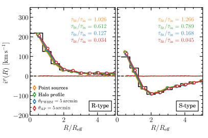
Figure 2: Left–the results for voids with $\lambda_{v}<10$ (R-type); Right– the results for voids with $\lambda_{v}>10$ (S-type). The black step line shows the theoretical radial velocity profile which is directly read from the simulated catalogue. The estimate radial velocity profiles with different stages of simulation maps are fit to the theoretical curve with $\bar{\tau}$ as the free fitting parameter. The ratio of the fitted $\bar{\tau}_{\rm fit}$ to input $\bar{\tau}_{\rm in}$ are also list, where $\bar{\tau}_{\rm in}\equiv 10^{-3}$. The dashed lines are the mean $\hat{v}^{\rm e}$ estimated with the pixels randomly-shuffled CMB temperature values (see Sect. (IV.2) for details).

We first calculate the radial velocity profile of cosmic voids as black step lines in Fig. 2. Since each void has different radius, we plot the radial velocity profile as a function of normalized radius $R/R_{\rm eff}$, where $R_{\rm eff}$ is the effective void radius. The void catalogue is split into R-type and S-type subsamples according the void parameter $\lambda_{v}$. The left panel of Fig. 2 shows the case with R-type voids ($\lambda_{v}<10$) and right panel shows the S-type voids ($\lambda_{v}>10$). One can see that, a significantly different radial velocity profiles between these two types are shown. The R-type voids have a positive velocity profile up to the radial distance of 5 times of void effective radius, indicating an overall expansion of the voids. The velocity profile of the S-type voids is positive within the void effective radius and negative outside, which indicates that at the boundary region the structures are actually collapsing. This velocity structure is consistent with the previous investigation of the radial density profile through numerical simulations  Sheth and van de Weygaert (2004); Paz et al. (2013); Demchenko et al. (2016).

We then test the behaviour of our estimator (Eqs. (11)-(13)) with simulated kSZ maps at the three different stages as mentioned in Sect. III.2 and Fig. 1. We first estimate the the voids expansion rate by using our estimator (Eq. (13)) and then fit the estimated $\tilde{v}^{\rm e}$ to the theoretical prediction with $\bar{\tau}$ as the free scaling parameter. The values of $\bar{\tau}_{\rm fit}/\bar{\tau}_{\rm in}$, which are the ratio of best-fitting to the initial input value of $\bar{\tau}_{\rm in}\equiv 10^{-3}$, are list in the legend with corresponding colors for each individual simulation stage.

The radial velocity profile estimated with the first stage simulation map, which assumes the cluster to be point sources, is shown with orange color. Both the results for R-type and S-type voids are fitted to the theoretical predictions very well. The values of $\bar{\tau}_{\rm fit}/\bar{\tau}_{\rm in}=1.026\pm 0.04$ for R-type of voids, which is consistent with unity. For S-type voids, $\bar{\tau}_{\rm fit}/\bar{\tau}_{\rm in}=1.266\pm 0.06$, which indicates a larger $\bar{\tau}$ comparing to the mean values. A possible reason is that, the S-type voids are mostly located in overdense region, where the $\bar{\tau}$ is over the global mean values.

The results with the simulation maps considering the halo profiles are shown as green lines; and the results with further including the beam smoothing effect are shown as blue lines. Both of these two sets of results are fitted to the theoretical predictions very well, except for the decreasing values of the $\bar{\tau}_{\rm fit}/\bar{\tau}_{\rm in}$. Therefore, both Gaussian profile and the beam effect can smooth the signal of the void expansion effect, producing a lower estimated value for the mean optical depth of clusters.

In the kSZ studies with real observational data, the primary fluctuation of the CMB is usually the contaminant factor at the background level. Therefore, the aperture photometry method (AP) is usually used as a filter to remove the long-wavelength mode fluctuations of the CMB Hernández-Monteagudo et al. (2015); De Bernardis et al. (2017); Li et al. (2018). In the AP method, we compute the average temperature within a given angular radius $\theta$ and subtract from it the average temperature in a surrounding ring with inner and outer radii $[\theta,\sqrt{2}\theta]$. This method is model-independent and blinds to any specific model of spatial distribution of gas. As suggested by Ref. Li et al. (2018), we use the aperture size $\theta_{\rm AP}=5\,$arcmin which can optimize the detection.

We apply the AP filter to our Stage-3 simulation and show the results in red lines in Fig. 2. One can see that the profile can be well fitted by the theoretical velocity profile, but the mean optical depth is reduced by almost $2$ orders of magnitude. The signal reducing due to the smoothing effect makes the detection harder if systematic noise, such as the equipment noise, CMB and thermal SZ residuals are presented.

IV Measurements with Planck maps

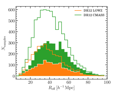
Figure 3: The empty histograms show the distribution of the total LOWZ/CMASS (orange/green) void catalogue; The filled histograms show the distribution of the void with $\lambda_{v}<10$ (R-type voids). The difference between empty and filled histograms is therefore for S-type voids, which have $\lambda_{v}>10$.

IV.1 Data

Here we present the real data in our estimation of radial velocity profile of cosmic voids.

Planck CMB maps

We use two different thermal SZ-free CMB maps in our study to cross-check the consistency. One is the 2D-ILC CMB map, which is obtained by applying the ‘Constrained ILC’ component separation method Remazeilles et al. (2011) to the public Planck 2015 data. This algorithm is similar to the Planck NILC method Delabrouille et al. (2009); Basak and Delabrouille (2012) which performs a minimum-variance weighted linear combination of the $9$ Planck frequency maps, with weights calculated to give response to CMB spectral distortion. In addition to this, the algorithm is designed to nullify the tSZ signal so there is no tSZ bias and variance in this map. The Full-Width-Half-Maximum (FWHM) of the map is $\theta_{\rm FWHM}=5\,$arcmin. For more details of the 2D-ILC map, we refer to Refs. Remazeilles et al. (2011) and Planck Collaboration et al. (2017).

As a comparison, we also use the SMICA-noSZ map from Planck survey Planck Collaboration et al. (2018) in this analysis. The Spectral Matching Independent Component Analysis (SMICA) method produces a foreground-cleaned CMB map from a linear combination of multi-frequency sky maps in harmonic space Cardoso et al. (2008). Similar to 2D-ILC map, this method also imposes a linear constraint to nullify the frequency dependence of the tSZ. The angular resolution of the SMICA-noSZ map is the same as 2D-ILC map.

The major difference between the two methods is that the 2D-ILC map uses wavelet decomposition to clean foregrounds locally both in pixel space and harmonic space, whereas the Planck SMICA-noSZ map is performed only in harmonic space. In addition, the 2D-ILC map was produced based on Planck 2015 data release, while the SMICA-noSZ map is based on Planck 2018 data release. Therefore, SMICA-noSZ map is less noisy and also has some improvements on calibrations of Planck instrumental systematics.

Central Galaxy Catalogue

We adopt the galaxy catalogue of the twelfth data release of the Baryon Oscillation Spectroscopic Survey (BOSS DR12) and further select the “Central Galaxies” from the catalogue. The BOSS sample is designed to measure the BAO signature in two-point correlation function of the galaxy clustering. The BOSS/DR12 catalogue is separated into “LOWZ” and “CMASS” catalogues. Both catalogues include two separated survey areas, located in Northern and Southern Galactic Caps (NGC and SGC). In our analysis, we combine NGC and SGC samples.

The “LOWZ” samples span the redshift below $0.45$; and the “CMASS” samples span the redshift between $0.45$ and $0.8$  Reid et al. (2016). We cut off samples with $z<0.01$. We further reduce the catalogue by choosing the “Central Galaxies” which are isolated and dominant galaxies with no other galaxies within $1.0\,{\rm Mpc}$ in the transverse direction and redshift difference smaller than $1,000\,{\rm km\,s}^{-1}$ Planck Collaboration et al. (2016c); Li et al. (2018). The selected central galaxies samples are regarded as the good indicator of the gravity center and therefore represent the clusters’ center positions. We refer the reader to Ref. Li et al. (2018) for more details of the selection process.

Void catalogue

The void catalogue used in our analysis are also generated with the BOSS DR12 LOWZ/CMASS LSS galaxy samples Nadathur (2016) and identified via REVOLVER void-finding algorithm, which is the same method as we used for our simulation void catalogue. The void size distribution of the LOWZ/CMASS void catalogue are shown in Fig. 3. The empty histograms in Fig. 3 show the void size distribution of the total void catalogue, with orange color for LOWZ catalogue and green color for CMASS catalogue, respectively. The size distribution of the R-type voids, which are void with $\lambda_{v}<10$ is shown with the filled histogram and the differences between empty and filled histogram show the distribution of S-type voids. One can see that for both R-type and S-type voids in both LOWZ and CMASS catalogues, the peak distribution of the void size is around $R_{\rm eff}\simeq 40\,h^{-1}{\rm Mpc}$. The total number of R-type and S-type voids for LOWZ are $1,462$ and $1,348$ and for CMASS are $3,845$ and $3,122$, shown in Table 1. This indicates that CMASS volume contains more voids than LOWZ volume, and within each survey volume there is similar number of R-type and S-type voids. There’s no significant difference in voids size distribution between R-type and S-type voids.

IV.2 Results of computation

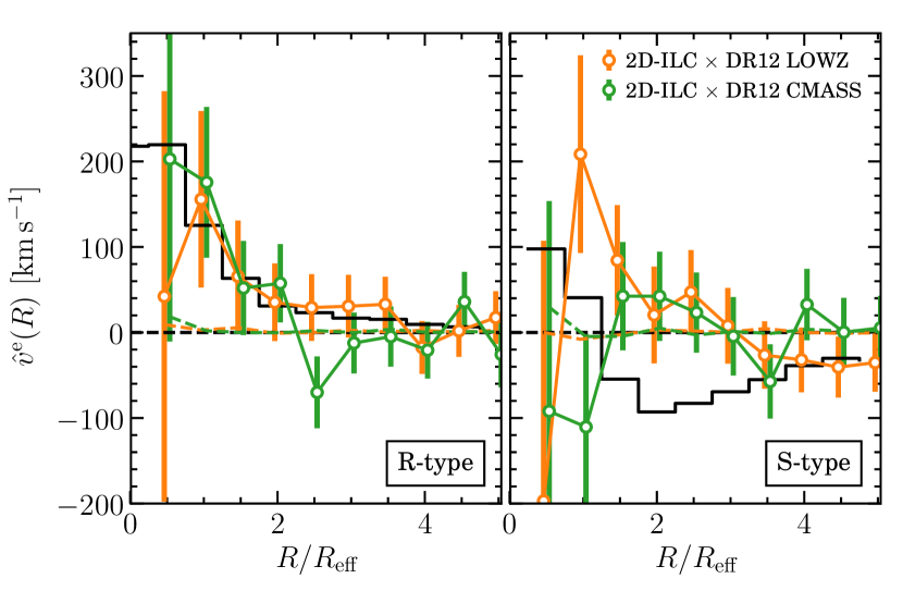
Figure 4: The estimated $\hat{v}^{\rm e}(R)$ with Planck 2D-ILC CMB map and LOWZ/CMASS (orange/green) void catalogue. The black step line shows the theoretical prediction which is directly read from the simulated catalogue. The left and right panels show the results for R-type and S-type voids, respectively. The estimated kSZ temperature difference are converted to velocity using Eq. (6). We use the $\bar{\tau}$ fitted with R-type results for both R-type and S-type temperature-velocity conversion. The fitted $\bar{\tau}$ values are summarized in Table 1.

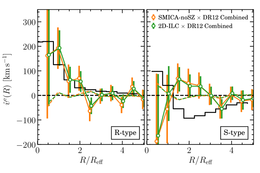
Figure 5: Same as Fig. 5, but using Planck SMICA-noSZ/2D-ILC maps (orange/green) and combined LOWZ and CMASS catalogue. We use the $\bar{\tau}$ fitted with R-type results for both R-type and S-type temperature-velocity conversion. The fitted $\bar{\tau}$ values are summarized in Table 1.

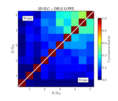
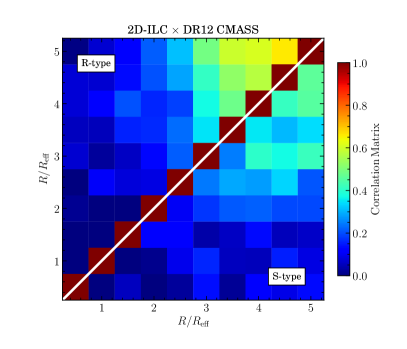
Figure 6: The correlation coefficient matrix for the measurements of Planck 2D-ILC map with DR12 LOWZ/CMASS void catalogue (top-left/right panels, respectively); and Planck SMICA-noSZ/2D-ILC map with combined DR12 LOWZ and CMASS void catalogue (bottom-left/right panels, respectively). In each panel, the upper triangle shows the correlation coefficient matrix of the R-type voids; and lower triangle shows the S-type.

The results estimated with the Planck 2D-ILC CMB map and LOWZ/CMASS galaxy and void catalogue are shown in Fig. 5. The black step line is the same as in Fig. 2, which is the theoretical prediction of the void expansion rate from simulation.

The error of the measurements is estimated by randomly-shuffling $N$ times the AP filtered CMB temperature values, which have galaxy samples located in. The AP filter is applied before shuffling pixels. With such mock samples, the voids relative position and involved galaxy number are kept the same, but the LSS correlation are broken due to the shuffling. The covariance matrix is then estimated as

$$C_{ij}^{\rm mock}=\frac{1}{N-1}\sum_{k=1}^{N}\left(\hat{v}_{k}^{\rm e}(R_{i})-\langle\hat{v}^{\rm e}(R_{i})\rangle\right)\left(\hat{v}_{k}^{\rm e}(R_{j})-\langle\hat{v}^{\rm e}(R_{j})\rangle\right)$$ (18)

in which $i$ and $j$ are the indices of the $R/R_{\rm eff}$ bins, in which we have $10$ radius bins in this study. $\hat{v}_{k}^{\rm e}(R)$ is the estimated radial velocity with the $k$-th mock void catalogue realization; $\langle\hat{v}^{\rm e}(R)\rangle$ is the mean of $N$ realizations and shown with the dashed lines in Fig. 5. We use $N=300$ in our analysis and confirm that the covariance estimation is converged for $N\geq 300$. The diagonal terms of the covariance matrix are used as the error of the measurements, shown in Figs. 5 and 2. The correlation coefficient matrix is then estimated via,

$$E_{ij}=\frac{C_{ij}^{\rm mock}}{\sqrt{C_{ii}^{\rm mock}C_{jj}^{\rm mock}}},$$ (19)

which is shown in Fig. 6. The correlation coefficient matrix for LOWZ and CMASS are shown in the left and right panels, respectively. In each panel, the results for R-type voids are shown in the upper triangle region; while the S-type voids are shown in the lower triangle region. As we can see, at the larger $R/R_{\rm eff}$ bins, the results are more correlated between bins. The correlation between bins is due to the sharing of galaxy samples between different voids. The galaxy samples located far from the void center have higher chance to be involved in different voids. Also we can see that the LOWZ samples are less correlated comparing to CMASS. It is because the CMASS samples are located at higher redshifts, and, given the similar voids size distribution between CMASS and LOWZ, galaxy samples at high redshift have more chance to be shared between voids.

The results for R-type voids ($\lambda_{v}<10$) are shown in the left panel. The estimated kSZ temperature difference are converted to velocity by using Eq. (6). The radial velocity profile for R-type voids is consistent with the theoretical predictions within the errors. The fitted $\bar{\tau}=(1.24\pm 0.79)\times 10^{-4}$ and $(0.87\pm 0.46)\times 10^{-4}$ for LOWZ and CMASS, respectively, which are consistent with the results measured with pairwise kSZ of clusters Li et al. (2018) within the error.

To quantify the level of detection, we define $\chi^{2}_{\rm NULL}$ and $\chi^{2}_{\rm reduced}$ as follows

$$\chi^{2}_{\rm NULL} =\sum_{ij}\hat{v}^{\rm e}(R_{i})\left(C^{-1}\right)_{ij}\hat{v}^{\rm e}(R_{j}),$$ (20)

$$\chi^{2}_{\rm reduced} =\chi^{2}_{\rm min}/{\rm d.o.f.}$$ (21)

where, ${\rm d.o.f.}=N_{\rm bins}-N_{\rm parameters}$, and

$$\chi^{2}_{\rm min}={\rm min}\left[\sum_{ij}\left(\hat{v}^{\rm e}(R_{i})-v^{\rm t}(R_{i})\right)\left(C^{-1}\right)_{ij}\left(\hat{v}^{\rm e}(R_{j})-v^{\rm t}(R_{j})\right)\right].$$ (22)

The $C^{-1}$ is the inverse of the covariance matrix. Besides the covariance matrix estimated with the mock void samples, we further include the covariance of the intrinsic error $C^{\rm intr}$, which is due to the intrinsic scattering of the velocity within the $R/R_{\rm eff}$ bins. The intrinsic covariance is estimated via velocities read directly from the simulation and it contributes $\lesssim 1\%$ of the uncertainties to the total variance. But when the variance is reduced by using more samples, the intrinsic variance contributes is up to $\lesssim 10\%$. Finally, we apply the Hartlap factor Hartlap et al. (2007) to correct the biased inverse covariance matrix. The $C^{-1}$ is finally defined as

$$C^{-1}=\frac{N-N_{\rm bin}-2}{N-1}\left(C^{\rm mock}+C^{\rm intr}\right)^{-1}.$$ (23)

Equation (20) quantifies the detection of the signal with respect to null, where indices $i$ and $j$ run over all radius bins; and Eq. (21) quantifies the goodness of fit. We summarize our quantification in Table 1.

IV.2.1 Null detection

In Figs. 5 and 5, we plot the reconstructed peculiar velocities $\hat{v}^{\rm e}(R)$ with Planck 2D-ILC and SMICA-noSZ maps and LOWZ/CMASS void catalogues. We list the detailed values of null detection for each respective case in Table 1. One can see that, for LOWZ catalogue, detection of R-type void is similar to the case of S-type void, and the $\chi^{2}_{\rm NULL}$ values are in the range of $7.11$ to $8.78$ depending on which CMB maps are used. One can further convert the $\chi^{2}_{\rm NULL}$ value into the “$p$-value”, which is defined as the probability of no detection given the measurement, i.e.

$$p={\rm Erfc}\left(\sqrt{\frac{\chi_{\rm NULL}^{2}}{2}}\right),$$ (24)

where “Erfc” is the complementary error function. Therefore, for LOWZ catalogue, the probability of null detection of R-type and S-type voids for using two different versions of Planck CMB map is at $5\times 10^{-3}$ level, indicating $\sim 3\sigma$ C.L. detection of the two types of voids.

For CMASS catalogue, the R-type void is better detected than the S-type void, due to its uniformly expanding structure. The detection of R-type void is boosted to $\chi^{2}_{\rm NULL}=17.79$ for 2D-ILC map and $14.69$ for SMICA-noSZ map. This corresponds to the $p-$value as $2.47\times 10^{-5}$ for 2D-ILC map and $1.27\times 10^{-4}$ for SMICA-noSZ map. For S-type void, the $\chi^{2}_{\rm NULL}$ is around $6.5$, which corresponds to $p=1.04\times 10^{-2}$.

In Table 1, we also list the $\chi^{2}_{\rm NULL}$ for the combined LOWZ and CMASS catalogues. For R-type void, by using 2D-ILC map it reaches $21.86$, and by using SMICA-noSZ map, it reaches $21.32$. These correspond to the $p-$values in the range of $(2.93-3.89)\times 10^{-6}$. The S-type void detection is reduced to $\chi^{2}_{\rm NULL}\simeq 6.1$ for the 2D-ILC map, for which $p-$value is $1.35\times 10^{-2}$.

To summarize, the probability of null detection for R-type and S-type voids are $2.93\times 10^{-6}$ and $1.35\times 10^{-2}$ for the Planck 2D-ILC map, so the R-type and S-type voids are detected at $3.31\sigma$ and $1.75\sigma$ C.L. respectively.

IV.2.2 Measuring expansion profile

For R-type voids, Planck 2D-ILC map gives $\chi^{2}_{\rm reduced}=(0.33\,,1.34\,,1.19)$ with the DR12-LOWZ, DR12-CMASS and the combination of such two voids catalogue, respectively. The lower $\chi^{2}_{\rm reduced}$ indicates that the results is over-fited. It might be because the signal is attenuated due to the smear effect of the large AP filter. We have $1.54\sigma$ (weak) detection of the $\bar{\tau}$ with LOWZ cataluge, $1.94\sigma$ with CMASS catalogue and $2.68\sigma$ with the combination of such two catalogues.

For S-type voids, the reconstructed velocity profile is biased and the fitted $\bar{\tau}$ is consistent with $0$. This large uncertainty of estimates is due to the instrumental noise, CMB residual and other residual foreground. The estimated results are shown in right panel of Fig. 5. The estimated kSZ temperature difference is also converted to velocity using Eq. (6). However, we use the fitted $\bar{\tau}$ with R-type voids, instead of the S-type voids. We also did the estimation by replacing the 2D-ILC map with SMICA-noSZ map and find very similar results to Fig. 5. We then combine the DR12 LOWZ and CMASS samples and stack the radial velocity profile against the 2D-ILC and SMICA-noSZ maps, and show in Fig. 5. One can see that the error-bars for both cases shrink and there is a clear detected signal for R-type of voids. For S-type of voids, there is still a large bias existed, due to its “cross-zero line” structure.

We then measure the value of optical depth ($\bar{\tau}$) by fitting the theoretical void expansion profile (black step line) to the data, and show our results in Table 1. The $\bar{\tau}$ value is measured to be $(1.03\pm 0.38)\times 10^{-4}$ for the R-type void, and $(-0.17\pm 0.24)\times 10^{-4}$ for the S-type void.

Table 1: The summary of the significance and bias of the reconstructed radial velocity profile of voids with Planck data.

LSS Tracer					Planck maps
					2D-ILC			SMICA-noSZ
SDSS Catalogue	$N_{\rm CG}$	Effective Area	Void type	$N_{\rm void}$	$\chi^{2}_{\rm NULL}$	$\chi^{2}_{\rm reduced}$	$\bar{\tau}\times 10^{4}$	$\chi^{2}_{\rm NULL}$	$\chi^{2}_{\rm reduced}$	$\bar{\tau}\times 10^{4}$
DR12-LOWZ	$386,603$	$7,943\deg^{2}$	R-type	$1,462$	$7.11$	$0.33$	$1.24\pm 0.79$	$7.68$	$0.35$	$1.30\pm 0.77$
			S-type	$1,348$	$8.78$	$0.98$	$-0.09\pm 0.41$	$7.71$	$0.85$	$-0.21\pm 0.38$
DR12-CMASS	$779,070$	$8,901\deg^{2}$	R-type	$3,845$	$17.79$	$1.34$	$0.87\pm 0.46$	$14.69$	$1.34$	$0.59\pm 0.45$
			S-type	$3,122$	$6.57$	$0.70$	$-0.12\pm 0.29$	$6.96$	$0.72$	$-0.17\pm 0.29$
Combined	$1,165,673$	$8,901\deg^{2}$	R-type	$5,307$	$21.86$	$1.19$	$1.03\pm 0.38$	$21.32$	$1.51$	$0.86\pm 0.38$
			S-type	$4,470$	$6.10$	$0.62$	$-0.17\pm 0.24$	$4.86$	$0.45$	$-0.22\pm 0.24$

V Forecast for future CMB experiments

V.1 CMB residuals

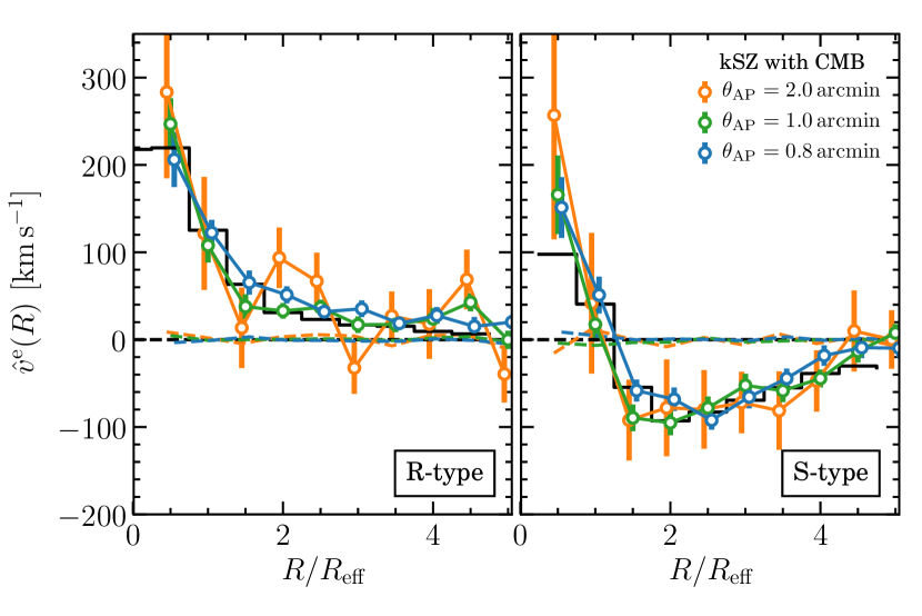
Figure 7: The simulated signal with added primary CMB as contaminations, assuming $2000\deg^{2}$ survey area and $\theta_{\rm FWHM}=1.4\,{\rm arcmin}$ resolution. The estimated $\hat{v}^{\rm e}(R)$ with different AP filter radii are shown with different colors.

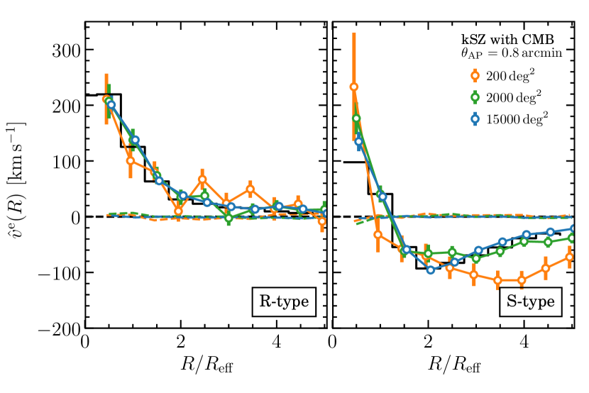
Figure 8: The simulated signal with CMB fluctuation residual as contaminations, assuming $\theta_{\rm FWHM}=1.4\,{\rm arcmin}$ resolution and $\theta_{\rm AP}=0.8\,{\rm arcmin}$ as filter radius. Different color indicate the results with different survey area.

The major contaminations to the signal come from the CMB temperature fluctuations, which are supposed to be filtered out with the designed filter. However, the residual of the CMB temperature fluctuation is still not negligible comparing to the relatively weak signal. In the meanwhile, the residual is also filter-parameter dependent. In this analysis, we focus on discussing the effect of the AP filter.

We add the simulated CMB temperature fluctuations to the signal map, which has resolution of $1.4\,{\rm armin}$ and the area of $2000\,{\rm deg}^{2}$. The AP filter is applied with filter radius sizes varying between $2\,{\rm arcmin}$, $1\,{\rm arcmin}$ and $0.8\,{\rm arcmin}$. The results are shown in Fig. 8. As shown in the figure, the measured $\tilde{v}^{\rm e}_{R}$ with $2\,{\rm arcmin}$ AP radius size (shown in orange color) has large errors. The errors are reduced with smaller AP filter radius size. With $2\,{\rm arcmin}$, $1\,{\rm arcmin}$ and $0.8\,{\rm arcmin}$ AP size, we achieve $2.93\sigma\,\,,7.68\sigma\,\,,9.11\sigma$ detection for R-type voids; and $3.63\sigma\,\,,11.82\sigma\,\,,11.40\sigma$ for S-type. The corresponding fitted $\bar{\tau}$ are $(2.26\pm 0.77\,\,,2.95\pm 0.38\,\,,3.51\pm 0.38)\times 10^{-4}$ for R-type voids ($\lambda_{v}<10$) and $(2.88\pm 0.79\,\,,5.12\pm 0.43\,\,,4.66\pm 0.41)\times 10^{-4}$ for S-type ($\lambda_{v}>10$). The smaller value of $\bar{\tau}$ with larger AP radius size is due to the smear effect of the AP filter.

In the mean while, an obvious bias is shown at some scales, especially with large AP filter size. With different simulation realizations, we found that the amplitude and scales of the bias are varying. A possible reason of the bias is the residual structures of the CMB temperature fluctuation. The larger the AP filter size, the more residual CMB temperature fluctuation are existed in the estimation. On the other hand, the bias is also dependent on the number of samples. To investigate how the bias are varying with voids sample, we use different effective area of the simulated catalog, assuming CMB map resolution of $1.4\,{\rm armin}$ and AP filter size of $0.8\,{\rm arcmin}$. The results are shown in Fig. 8. The green data in Fig. 8 shows the results assuming $2,000\deg^{2}$ survey area, which includes $410$ R-type and $174$ S-type voids; The orange ones are the results by selecting only $10\%$ of the survey area as the green ones, corresponding to reduce the survey area to $200\deg^{2}$ and including $36$ R-type and $20$ S-type voids; The blue data are the results with $15,000\deg^{2}$, including $3,002$ R-type and $1,403$ S-type voids. With the survey area varied from $200\deg^{2}$, $2,000\deg^{2}$ to $15,000\deg^{2}$, the $\chi^{2}_{\rm reduced}$ vary from $1.81$, $0.98$ to $1.11$ for the R-type voids, and from $3.94$, $1.47$ to $0.98$ for the S-type voids. Given the ${\rm d.o.f}=9$, a $\chi^{2}_{\rm reduced}=1.00\pm 0.47$ indicates a good fit.

V.2 Future experiments

Table 2: Forecasts for ACT, AdvACT and Simons Observatory detection of voids profile. The results with $\sigma_{n}=0$ is the instrumental noise free case.

Survey Area [deg2]	$N_{\rm CG}$	$\sigma_{\rm n}$ [$\mu$K-arcmin]	Void type	$N_{\rm void}$	$\chi^{2}_{\rm NULL}$	$\chi^{2}_{\rm reduced}$	$\bar{\tau}\times 10^{4}$	Experiments
$2,000$	$50,250$	$0$	R-type	$410$	$147.91$	$0.98$	$3.51\pm 0.38$	SPT-3G
			S-type	$174$	$119.77$	$1.47$	$4.66\pm 0.41$
		$10$	R-type	$410$	$45.46$	$0.94$	$4.30\pm 1.18$
			S-type	$174$	$26.68$	$1.42$	$5.38\pm 1.27$
$15,000$	$394,155$	$20$	R-type	$3002$	$26.79$	$0.84$	$3.03\pm 0.89$	Pessimistic AdvACT
			S-type	$1403$	$36.76$	$1.65$	$3.87\pm 0.82$
		$10$	R-type	$3002$	$97.43$	$1.39$	$3.60\pm 0.51$	Simons O./AdvACT
			S-type	$1403$	$47.05$	$0.82$	$3.22\pm 0.46$
		$6$	R-type	$3002$	$204.49$	$1.03$	$3.65\pm 0.34$	Optimistic Simons O./AdvACT
			S-type	$1403$	$133.48$	$1.89$	$3.68\pm 0.31$

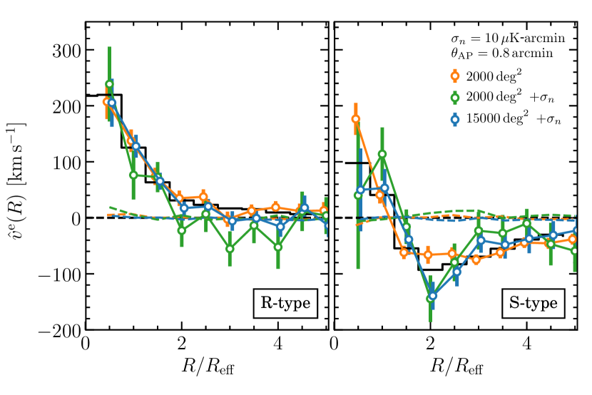
Figure 9: The simulated signal with CMB fluctuation residual and thermal noise of $10{\rm\mu K\raisebox{0.75pt}{-}arcmin}$, assuming $\theta_{\rm FWHM}=1.4\,{\rm arcmin}$ resolution and $\theta_{\rm AP}=0.8\,{\rm arcmin}$ AP filter radius. The result with $2,000\deg^{2}$ and $15,000\deg^{2}$ survey area are shown with different colors.

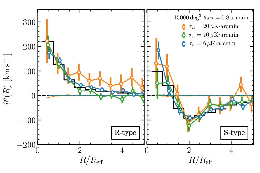
Figure 10: The simulated signal with CMB fluctuation residual and thermal noise, assuming $\theta_{\rm FWHM}=1.4\,{\rm arcmin}$ resolution and $\theta_{\rm AP}=0.8\,{\rm arcmin}$ as filter radius. Different colors indicate the results with different thermal noise level.

The sensitivity and angular resolution of CMB experiments are being improved rapidly, with several on-going ground-based CMB observatories, such as SPT-3G Benson et al. (2014a), ACT Hilton et al. (2018), AdvACT Benson et al. (2014b); Suzuki et al. (2016); Henderson et al. (2016), and Simons Observatory Ade et al. (2019). These ground-based CMB surveys will provide higher angular resolution CMB maps with lower noise levels in the near future. Here we plan to simulate the future detectability of ACT, AdvACT and Simons Observatory, by assuming that the angular resolution of these survey can reach $\theta_{\rm FWHM}=1.4\,$arcmin. We assume that SPT-3G will cover $2,000\,{\rm deg}^{2}$ survey area, AdvACT and Simons Observatory will cover $15,000\,{\rm deg}^{2}$ area, respectively Ade et al. (2019). The latter one corresponds to the $f_{\rm sky}\simeq 0.4$ but excluding Galactic plane. Beside the CMB temperature fluctuation, we further add instrumental noises at different level according to different CMB experiments. We assume $10\,\mu{\rm K}\raisebox{0.75pt}{-}$arcmin rms noise for SPT-3G. For AdvACT, the rms noise level is around 10 to 20 $\mu{\rm K}\raisebox{0.75pt}{-}$arcmin so we assume that $\sigma_{\rm n}=20\,\mu{\rm K}\raisebox{0.75pt}{-}$arcmin as pessimistic case, and $\sigma_{\rm n}=10\,\mu{\rm K}-$arcmin as optimistic case. For Simons Observatory, we assume $\sigma_{\rm n}=10\,\mu{\rm K}\raisebox{0.75pt}{-}$arcmin as pessimistic case and $\sigma_{\rm n}=6\,\mu{\rm K}\raisebox{0.75pt}{-}$arcmin as optimistic case as indicated in Ref. Ade et al. (2019). The results are shown in Figs. 10 and 10; and the fitting values are summarized in Table 2.

Figure 10 shows the results with rms $=10\,\mu{\rm K}\raisebox{0.75pt}{-}{\rm arcmin}$ noise added. The result with noise free is shown in orange color and the result with $2,000\deg^{2}$ survey area is shown in green. Although the estimated $\bar{\tau}$ is consistent with each other, the error is increased from $0.38(0.41)\times 10^{-4}$ to $1.18(1.27)\times 10^{-4}$ for R-type (S-type) voids. Even though the error is increased by a factor of $3$, the further CMB experiments such as SPT-3G can still achieve $3.65\sigma(4.22\sigma)$ detection with $2,000\deg^{2}$ survey area.

If the survey area can be extended to $15,000\deg^{2}$, the estimation uncertainty can be reduced significantly. In the case of pessimistic case of AdvACT experiments, one can still achieve $3.4\sigma(4.73\sigma)$ detection for R-type (S-type) voids with noise rms$=20\,\mu{\rm K}\raisebox{0.75pt}{-}{\rm arcmin}$. With the optimistic AdvACT experiment or the pessimistic Simons Observatory, by assuming noise rms$=10\,\mu{\rm K}\raisebox{0.75pt}{-}{\rm arcmin}$, the detection can be improved to about $7\sigma$ for both R-type and S-type voids. With further optimistic case of noise rms$=6\,\mu{\rm K}\raisebox{0.75pt}{-}{\rm arcmin}$ for Simons Observatory, one can potentially achieve $\sim 10.7\sigma$ (R-type) and $11.8\sigma$ (S-type) detections with our estimator.

VI Conclusion

In this paper, we develop an estimator to extract the mean radial velocity profile of the voids via the kinematic Sunyaev-Zeldovich effect of pairs of galaxies around the voids. We firstly test the estimator with the simulated pure kSZ maps, which are constructed from the BigMD $N$-body simulation Klypin et al. (2016); Prada et al. (2012) and the void catalogue generated with the same simulation. The estimator is tested with the R-type and S-type voids separately and the results show that the mean radial velocity profile can be fully recovered with our estimator. With the simulated kSZ map, we note that the recovered signal is highly attenuated with the lower angular resolution of the map or larger AP filter radius size, leading to the potential bias of optical depth.

We apply the estimator to the Planck 2D-ILC CMB map, with the LOWZ/CMASS galaxy and void catalogue. We conducted two statistics for the measured expansion profile of the void. One is the $\chi_{\rm NULL}^{2}$ for NULL detection, which is calculated as the data against the zero line; the other is the $\chi^{2}_{\rm reduced}$ which is calculated as the minimal $\chi^{2}$ value between the data and the best-fitting theoretical profile. For the R-type and S-type voids, $\chi^{2}_{\rm NULL}$ is calculated as $21.86$ and $6.10$ for the 2D-ILC map, which corresponds to the probability of $2.93\times 10^{-6}$ and $1.35\times 10^{-2}$ of null detection. This suggests that the R-type and S-type voids are measured at $3.31\sigma$ and $1.75\sigma$ C.L. respectively.

We also calculate the $\chi^{2}_{\rm reduced}$ value as the minimal $\chi^{2}$ of the data with respect to the theoretical expansion profile. For R-type voids, the $\chi^{2}_{\rm reduced}=(0.33\,,1.34\,,1.19)$ with the DR12-LOWZ, DR12-CMASS and the combination of such two voids catalogue, respectively. We have $1.54\sigma$ measurement of the optical depth $\bar{\tau}$ with LOWZ cataluge, $1.94\sigma$ with CMASS catalogue and $2.68\sigma$ with the combination of such two catalogue. For the S-type voids, the measured $\bar{\tau}$ value is still consistent with $0$.

We further investigate the effect of the CMB temperature fluctuation contamination, by adding simulated CMB map to the kSZ simulation map. The AP filter is applied to the simulated map. The results show that the CMB temperature fluctuation residual can increase the uncertainty of estimation and bias the results. The uncertainty and bias can be reduced with smaller angular size of AP filter and larger amount of voids samples.

Finally, we forecast the detection for a few future CMB experiments with higher angular resolution and lower thermal noise. Beside the CMB contamination, we further add the instrumental noise at different level. The forecasts show that, experiment like SPT-3G can obtain $3.65\sigma(4.22\sigma)$ detection with $2,000\deg^{2}$ survey area at rms=$10\,\mu{\rm K}\raisebox{0.75pt}{-}{\rm arcmin}$; With $15,000\deg^{2}$ survey area, experiment like AdvACT can obtain $3.4\sigma(4.73\sigma)$ detection for R-type (S-type) voids with noise rms$=20\,\mu{\rm K}\raisebox{0.75pt}{-}{\rm arcmin}$; or about $7\sigma$ for both R-type and S-type voids at noise level of rms $=10\,\mu{\rm K}\raisebox{0.75pt}{-}{\rm arcmin}$. Finally, in the case of rms $=6\,\mu{\rm K}\raisebox{0.75pt}{-}{\rm arcmin}$, which is the most optimistic case of Simons Observatory, one can achieve over $10\sigma$ detection. Since the cosmic void is the most abundant structures of the large-scale Universe, our estimator opens a new window of probing dynamics of cosmic structures through the measurement of kinetic Sunyaev-Zeldovich effect.