Detection of PAH Absorption and Determination of the Mid-Infrared Diffuse Interstellar Extinction Curve from the Sightline Toward Cyg OB2-12

Abstract

The sightline toward the luminous blue hypergiant Cyg OB2-12 is widely used in studying interstellar dust on account of its large extinction ($A_{V}\simeq 10$ mag) and the fact that this extinction appears to be dominated by dust typical of the diffuse interstellar medium. We present a new analysis of archival ISO-SWS and Spitzer IRS observations of Cyg OB2-12 using a model of the emission from the star and its stellar wind to determine the total extinction $A_{\lambda}$ from 2.4–37 $\mu$m. In addition to the prominent 9.7 and 18 $\mu$m silicate features, we robustly detect absorption features associated with polycyclic aromatic hydrocarbons (PAHs), including the first identification of the 7.7 $\mu$m feature in absorption. The 3.3 $\mu$m aromatic feature is found to be much broader in absorption than is typically seen in emission. The 3.4 and 6.85 $\mu$m aliphatic hydrocarbon features are observed with relative strengths consistent with observation of these features on sightlines toward the Galactic Center. We identify and characterize more than sixty spectral lines in this wavelength range, which may be useful in constraining models of the star and its stellar wind. Based on this analysis, we present an extinction curve $A_{\lambda}/A_{2.2\,\mu{\rm m}}$ that extrapolates smoothly to determinations of the mean Galactic extinction curve at shorter wavelengths and to dust opacities inferred from emission at longer wavelengths, providing a new constraint on models of interstellar dust in the mid-infrared.

1 Introduction

Vibrational modes in the molecular constituents of interstellar grains give rise to a number of infrared features seen in extinction and emission. Notable among these are the infrared emission features attributed to polycyclic aromatic hydrocarbons (PAHs, Leger & Puget, 1984; Allamandola et al., 1985), some of which have also been detected in extinction (e.g., Schutte et al., 1998; Chiar et al., 2013), and the prominent 9.7 and 18 $\mu$m features arising from the Si-O stretching mode and O-Si-O bending mode in amorphous silicates, respectively (Woolf & Ney, 1969; van Breemen et al., 2011). Because of their identification with specific materials, these features enable detailed study of the chemical composition of grains as well as composition-specific properties, such as alignment efficiency.

Precise measurement of extinction by dust in the diffuse interstellar medium (ISM) at infrared wavelengths is an observational challenge. The mid-infrared (MIR) wavelengths central to this work are well into the Rayleigh-Jeans portion of stellar emission spectra, rendering most stars quite faint. Further, typical $\sim 0.1\,\mu$m interstellar grains are far more efficient in extinguishing UV and optical radiation than infrared, resulting in a weak signal unless much dust is present. Most sightlines with high visual extinction $A_{V}$ pass through dense molecular material where the dust differs from that found in the diffuse ISM, due for instance to the presence of ice mantles.

The sightline toward the luminous blue hypergiant Cyg OB2-12 (also known as Schulte 12) is frequently employed in studies of infrared extinction as it mitigates a number of these difficulties. One of the most intrinsically luminous stars in the Galaxy, Cyg OB2-12 lies behind $\sim 10$ magnitudes of visual extinction (Humphreys, 1978; Torres-Dodgen et al., 1991), allowing infrared extinction to be measured with high signal to noise. Additionally, the bulk of the extinction appears to originate from dust in the diffuse ISM rather than dense gas, as evidenced by a typical extinction curve and a lack of strong ice features (Whittet, 2015). Thus, this sightline has long been used to study the silicate features and the composition of interstellar silicates (Rieke, 1974; Adamson et al., 1990; Whittet et al., 1997; Schutte et al., 1998; Fogerty et al., 2016).

Despite these advantages, the unusual nature of Cyg OB2-12 also presents a number of modeling challenges. Photometric variability has been observed on short ($\lesssim$ 1 month) timescales in the X-ray (Rauw, 2011), optical (Nazé et al., 2019), and radio (Scuderi et al., 1998; Morford et al., 2016). A recently-discovered companion (Caballero-Nieves et al., 2014; Maryeva et al., 2016), though too faint to be detected in spectral features, raises the possibility of colliding stellar winds producing a significant fraction of the observed radio emission (Oskinova et al., 2017). Despite considerable effort modeling the panchromatic spectrum of Cyg OB2-12 (e.g., Clark et al., 2012), fundamental uncertainties about the precise nature of this source and its emission remain (see Nazé et al., 2019, for a recent discussion).

We focus in this work on modeling the MIR emission to derive the wavelength-dependent extinction from 2.4–37 $\mu$m. Over this wavelength range, we employ physically-motivated parametric models of the stellar continuum emission and free-free emission from the stellar wind, as well as knowledge of the properties of interstellar dust, to infer the absolute interstellar extinction on this sightline. The resulting extinction curve, which includes prominent features associated with both silicate and carbonaceous grains, is presented as a benchmark for models of interstellar dust at MIR wavelengths.

This paper is organized as follows: in Section 2, we describe the data used in this work; in Section 3, we present the models of the star, stellar wind, and spectral lines employed; the resulting extinction curve is derived in Section 4 and the identification and characterization of various extinction features is presented in Section 5; we discuss the implications of this work for dust models and potential directions for follow-up in Section 6; and finally, we summarize our principal conclusions in Section 7.

2 Data

2.1 MIR Spectroscopy

2.2 ISO-SWS

Cyg OB2-12 was observed in three different epochs with the Short Wavelength Spectrometer (SWS) aboard the Infrared Space Observatory (ISO). Three Astronomical Observing Template 1 (AOT1) spectra are available from the NASA/IPAC Infrared Science Archive having Target Dedicated Time numbers of 03602226, 13901048, and 33504130, corresponding to observations in December 1995, April 1996, and October 1996, respectively. These have been reduced as described in Sloan et al. (2003). Because the detector type, noise properties, and relative agreement between these spectra all change longward of 4.08 $\mu$m, for continuum measurements we analyze only the 2.35–4.08 $\mu$m data, although longer wavelength ISO data are used in emission line characterization (see Section 3.2). For more details on the SWS, see de Graauw et al. (1996).

To improve the relative agreement between spectra, we multiply the 03602226 and 33504130 spectra by factors of 0.976 and 0.935, respectively. After this correction, the three spectra agree to within $\sim 3$% over the range of interest, with only small systematic trends with wavelength appearing at either end of the range.

The December 1995 spectrum (03602226), taken during ISO commissioning, has both the shortest duration at 18 minutes and lowest spectral resolution ($R\sim 200$; Whittet et al., 1997). While the other two spectra are of comparable duration ($\sim$1 hour) and were taken at scan speed 3, affording higher spectral resolution, the April 1996 data (13901048) have more than twice the signal to noise over most of the wavelength range we consider. We therefore focus our analysis on this spectrum exclusively.

2.2.1 Spitzer IRS

Cyg OB2-12 is one of 159 stars that compose the Spitzer Atlas of Stellar Spectra (SASS), a set of prototype stellar spectra taken by the Spitzer Infrared Spectrograph (IRS) that have been reduced in a homogeneous way (Ardila et al., 2010). The SASS Cyg OB2-12 spectrum is a synthesis of two observations, one in October 2004 (AOR 9834496) and the other in August 2008 (AOR 27570176), that include data from both the Short-Low and High-Low modules (for more details on the IRS, see Houck et al., 2004). Together, these provide full spectral coverage from 5.2 to 35 $\mu$m. While we employ the IRS spectrum of Cyg OB2-12 from SASS, Fogerty et al. (2016) find that their alternative reduction based on the same data is in overall good agreement with the SASS spectrum. We retain the full SASS spectrum in all plots, however we exclude data having $\lambda<5.8\,\mu$m from our analysis since the spectrum in this region has relatively low signal to noise and differs qualitatively from the reduction of Fogerty et al. (2016).

The October 2004 IRS observation (AOR 9834496) also includes a high resolution spectrum ($R\sim 600$) from 10–37 $\mu$m. We employ these data as obtained from the Cornell Atlas of Spitzer/Infrared Spectrograph Sources (CASSIS) using the optimal differential extraction (Lebouteiller et al., 2015). To ameliorate the discontinuity in flux densities between the short-high (SH) and long-high (LH) modules at 19.5 $\mu$m, as well as to improve agreement with the SASS spectrum, we scale the SH data uniformly up by a factor of 1.06.

2.3 UV, Optical, and Infrared Photometry

Table 1: Cyg OB2-12 Continuum Fluxes

Assorted UV–NIR Photometry
Band	$\lambda$	$m_{X}$	$F_{\nu}\left(m_{X}=0\right)$	$F_{\nu}^{\rm model}$	$A_{\lambda}$	Reference
	[$\mu$m]	[mag]	$[{\rm Jy}]$	$[{\rm Jy}]$	[mag]
$U$	0.366	17.15	1790	1000	16.52	Wisniewski et al. (1967)
$B$	0.438	14.70	4063	945	13.12	Wisniewski et al. (1967)
$V$	0.545	11.48	3636	816	9.86	Wisniewski et al. (1967)
$R$	0.641	8.26	3064	702	6.66	Wisniewski et al. (1967)
$I$	0.798	5.95	2416	547	4.34	Wisniewski et al. (1967)
$J$	1.22	4.38	1589	308	2.60	Rieke & Lebofsky (1985)
$H$	1.63	3.28	1021	200	1.51	Rieke & Lebofsky (1985)
$K$	2.19	$2.715\pm 0.02$	640	127	0.96	Harris et al. (1978)
$L$	3.45	2.217	285	63.2	0.58	Harris et al. (1978)
$L^{\prime}$	3.80	2.17	238	54.5	0.57	Torres-Dodgen et al. (1991)
APASS Photometry (Henden et al., 2016)
Band	$\lambda$	$m_{X}$	$F_{\nu}\left(m_{X}=0\right)$	$F_{\nu}^{\rm model}$	$A_{\lambda}$
	[$\mu$m]	[mag]	$[{\rm Jy}]$	$[{\rm Jy}]$	[mag]
$B$	0.438	14.929	4063	945	13.35
$g$	0.4770	13.44	3631	900	11.93
$V$	0.545	11.58	3636	816	9.96
$r$	0.6231	10.196	3631	722	8.44
Gaia Photometry (Gaia Collaboration et al., 2018)
Band	$\lambda_{0}$	Flux		Model Flux		$A_{\lambda_{0}}$
	[nm]	[photoelectrons s-1]		[photoelectrons s-1]		[mag]
$G_{\rm BP}$	513.11	$3.11\times 10^{5}$		$3.40\times 10^{9}$		10.96
$G$	640.50	$5.25\times 10^{6}$		$4.28\times 10^{9}$		8.14
$G_{\rm RP}$	777.76	$8.48\times 10^{6}$		$1.76\times 10^{9}$		5.98
NIR–MIR Photometry from Leitherer et al. (1982)
Band	$\lambda$	$m_{X}$	$F_{\nu}\left(m_{X}=0\right)$	$F_{\nu}^{\rm model}$	$A_{\lambda}$
	[$\mu$m]	[mag]	$[{\rm Jy}]$	$[{\rm Jy}]$	[mag]
$H$	1.67	$3.33\pm 0.01$	1076	193	1.46
$K$	2.30	$2.72\pm 0.01$	598	118	0.96
$L$	3.57	$2.28\pm 0.02$	277	60.0	0.62
$M$	4.97	$2.06\pm 0.02$	158	36.0	0.45
$N$	10.9	$1.95\pm 0.07$	33	9.65	0.61

Table 1 presents a heterogeneous collection of photometric observations of Cyg OB2-12 from the literature. We adopt a representative set of $UBVRIJHKLL^{\prime}$ photometry from Wisniewski et al. (1967), Rieke & Lebofsky (1985), Harris et al. (1978), and Torres-Dodgen et al. (1991). A more complete compilation of historical data can be found in Clark et al. (2012). We note that Nazé et al. (2019) demonstrate optical variability of Cyg OB2-12 in the V band at the 0.1 mag level on a one year timescale using data from ASAS-SN (Kochanek et al., 2017) and a private observatory. Thus, multi-epoch comparisons are subject to uncertainties in excess of the formal photometric errors.

We supplement these data with observations from the AAVSO Photometric All Sky Survey (APASS) DR9 (Henden et al., 2016), Gaia DR2 (Gaia Collaboration et al., 2018), and Leitherer et al. (1982). All data, including the adopted zero levels, are listed in Table 1.

2.4 Radio Observations

Table 2: Cyg OB2-12 Radio Fluxes

$\lambda$	Date	$F_{\nu}$	Reference
$[{\rm cm}]$		$[{\rm mJy}]$
0.7	April 1995	$22.9\pm 0.6$	Contreras et al. (1996)
0.7	June 1999	$9.0\pm 1.5$	Contreras et al. (2004)
2	April 1995	$11.3\pm 0.1$	Contreras et al. (1996)
2.1	Sep. 1994	$7.70\pm 0.30$	Scuderi et al. (1998)
2.1	Oct. 1994	$12.0\pm 0.20$	Scuderi et al. (1998)
3.5	April 1995	$7.18\pm 0.04$	Contreras et al. (1996)
3.5	Sep. 1994	$4.74\pm 0.14$	Scuderi et al. (1998)
3.5	Oct. 1994	$7.40\pm 0.08$	Scuderi et al. (1998)
3.6	May 1993	$6.06\pm 0.07$	Waldron et al. (1998)
3.6	June 1999	$5.9\pm 0.1$	Contreras et al. (2004)
6	April 1995	$3.64\pm 0.12$	Contreras et al. (1996)
6	May 1993	$3.94\pm 0.07$	Waldron et al. (1998)
6	June 1999	$4.2\pm 0.1$	Contreras et al. (2004)
6.2	Sep. 1994	$4.00\pm 0.20$	Scuderi et al. (1998)
6.2	Oct. 1994	$5.03\pm 0.10$	Scuderi et al. (1998)
21	April 2014	$1.013\pm 0.055$	Morford et al. (2016)
21	April 2014	$0.598\pm 0.061$	Morford et al. (2016)

Cyg OB2-12 has been studied extensively at radio wavelengths. Table 2 presents a selection of these observations, which are plotted in Figure 1. The presented data were taken both with the Very Large Array (Contreras et al., 1996; Scuderi et al., 1998; Waldron et al., 1998; Contreras et al., 2004) and with e-MERLIN (Morford et al., 2016). Considerable variability is evident on both short ($\lesssim$ one month) and long ($\sim$years) timescales.

3 Model

Figure 1: In the left panel, we present our model of the flux from Cyg OB2-12 (black solid), including contributions from the stellar disk (blue dotted) and stellar wind (green dot-dashed). The Spitzer IRS spectrum of Cyg OB-12 is plotted in black after removal of the emission lines (see Figure 2). The Clark et al. (2012) model is plotted (red dashed) for comparison. In the right panel, we compare our model (black solid) and the Clark et al. (2012) model (red dashed) to observations of the radio continuum. We posit that free-free emission from the stellar wind of Cyg OB2-12 is a subdominant component of the observed radio flux.

3.1 Free-Free Emission from a Stellar Wind

The spectrum of a star with an ionized wind is discussed by Panagia & Felli (1975) and Wright & Barlow (1975), and Clark et al. (2012) present a model for emission from Cyg OB2-12. Our model builds on these results.

Let $R_{0}$ be the stellar radius, $D$ the distance, and $\theta_{\star}\equiv R_{0}/D$. We adopt the distance $D=1.75$ kpc estimated by Clark et al. (2012), which is consistent with the Gaia DR2 distances for the main Cygnus OB2 group (Berlanas et al., 2019). Cyg OB2-12 has an effective temperature $T_{\rm eff}\approx 13700$ K (Clark et al., 2012).

Assume that there is an ionized wind at $r>R_{0}$ with electron temperature $T_{w}$ and electron density $n_{e}(r)$. Let the total flux density from the star and wind be

$$F_{\nu}=F_{\nu}^{\star}+F_{\nu}^{\rm wind}~{}~{},$$ (1)

where $F_{\nu}^{\star}$ is the flux density from the stellar disk (impact parameters $b<R_{0}$) and $F_{\nu}^{\rm wind}$ is the flux density from impact parameters $b>R_{0}$. The “stellar” flux $F_{\nu}^{\star}$ includes the effects of radiative transfer through the wind projected in front of the stellar surface.

We assume the flux emerging from the photosphere to be a dilute blackbody, with dilution factor $\epsilon_{\star}=0.75$ and temperature $T_{\star}=T_{\rm eff}\epsilon_{\star}^{-1/4}=14700$ K. This dilution factor reproduces the MIR flux of an ATLAS9 model atmosphere having $T_{\rm eff}=14000$ K and $g=10^{2}$ cm s^-1 (Castelli & Kurucz, 2003).

Following Clark et al. (2012), we consider steady mass-loss $\dot{M}$ with electron density

$$n_{e}(r) =n_{e0}\left(\frac{R_{0}}{r}\right)^{2}\left(1-0.913{\frac{R_{0}}{r}}\right)^{-3}$$ (2)

$$n_{e0} \equiv\frac{\dot{M}/1.4m_{\rm H}}{4\pi R_{0}^{2}v_{\infty}}$$ (3)

and adopt $v_{\infty}=400$ km s^-1. At infrared and far-infrared wavelengths, the dominant opacity in the wind is free-free absorption, with attenuation coefficient

$$\kappa_{\nu}^{\rm ff} =An_{e}^{2}$$ (4)

$$A =3.69\times 10^{-21}T_{4}^{-1/2}\nu_{9}^{-3}g_{\rm ff}(\nu)\left[1-e^{-h\nu/kT_{w}}\right]\,{\rm cm}^{5}~{}~{},$$ (5)

where $T_{4}\equiv T_{w}/10^{4}$ K, $\nu_{9}\equiv\nu/10^{9}$ Hz, and $g_{\rm ff}(\nu)$ is the free-free Gaunt factor, approximated using Eq. (10.9) from Draine (2011). We take $T_{w}\approx T_{\star}$. At impact parameter $b\equiv\beta R_{0}$ (with $\beta>1$) the optical depth in the wind is

$$\tau_{\nu}(\beta\geq 1) =\int_{-\infty}^{\infty}\kappa_{\nu}^{\rm ff}\left(r=\sqrt{\beta^{2}R_{0}^{2}+x^{2}}\right)dx$$ (6)

$$=An_{e0}^{2}R_{0}\int_{-\infty}^{\infty}\frac{\left(\beta^{2}+u^{2}\right)du}{\left(\sqrt{\beta^{2}+u^{2}}-0.913\right)^{6}}~{}~{}.$$ (7)

For an isothermal wind,

$$F_{\nu}^{\rm wind}(\nu)=B_{\nu}(T_{w})\pi\theta_{\star}^{2}\int_{1}^{\infty}2\beta d\beta\left[1-e^{-\tau_{\nu}(\beta)}\right]~{}~{}.$$ (8)

For impact parameter $b<R_{0}$, the median optical depth in front of the stellar disk is

$$\tau_{\nu}^{m} =\int_{0}^{\infty}\kappa_{\nu}^{\rm ff}\left(r=\sqrt{R_{0}^{2}+x^{2}+xR_{0}\sqrt{2}}\right)dx$$ (9)

$$=5.911\times 10^{4}An_{e0}^{2}R_{0}$$ (10)

for the density profile (2). We take

$$F_{\nu}^{\star}\approx\pi\theta_{\star}^{2}B_{\nu}(T_{\star})\left[\epsilon_{\star}e^{-\tau_{\nu}^{m}}+(1-e^{-\tau_{\nu}^{m}})\right]~{}~{}~{}.$$ (11)

With this formulation, the continuum emission from the star and wind is set by only two free parameters: the angular size of the star $\theta_{\star}$ and the mass loss rate $\dot{M}$. We determine best-fit values of these parameters in Section 4 on the basis of the resulting extinction curve.

3.2 Line Emission

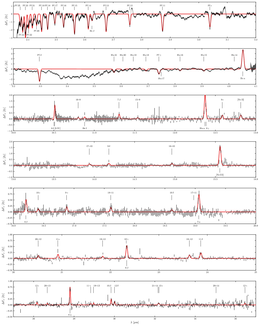
Figure 2: Absorption and emission lines seen in the ISO-SWS spectrum (top two panels) and the high resolution Spitzer IRS spectrum (bottom five panels). A simple model fit employing Gaussian line profiles is presented in red, with the corresponding equivalent widths listed in Table 3.

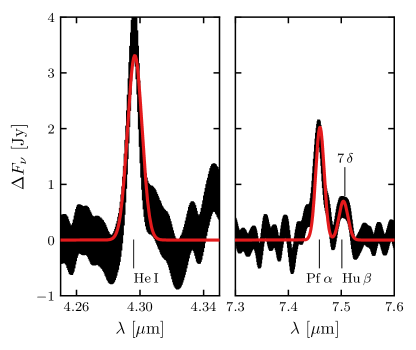
Figure 3: ISO-SWS spectrum relative to the continuum in the vicinity of the He I 4.296 $\mu$m and Pf $\alpha$ emission lines (left and right panels, respectively). The subdominant emission feature at 7.50–7.51 $\mu$m is a combination of the Hu $\beta$ and $7\delta$ lines. Equivalent widths corresponding to the model fit (red) are given in Table 3.

Table 3: Cyg OB2-12 Spectral Lines

ISO-SWS					Spitzer IRS
Name	$\lambda_{0}$	$n_{u}$	$n_{l}$	$W_{\lambda}$	Name	$\lambda_{0}$	$n_{u}$	$n_{l}$	$W_{\lambda}$
	[$\mu$m]			[Å]		[$\mu$m]			[Å]
Pf 25	2.374	25	5	$1.55$	8$\delta$	10.502	12	8	$11^{\dagger}$
Pf 24	2.382	24	5	$2.26$	[S IV]	10.511			$-46^{\dagger}$
Pf 23	2.392	23	5	$3.03$	16–9	10.802	16	9	$-3$
Pf 22	2.403	22	5	$1.84$	He I	10.881	1s4p	1s4s	$-6$
Pf 21	2.416	21	5	$1.80$	7$\beta$	11.307	9	7	$-15$
Pf 20	2.431	20	5	$1.49$	15–9	11.537	15	9	$-3$
Pf 19	2.449	19	5	$2.31$	Hu $\alpha$	12.370	7	6	$-84^{\dagger}$
Pf 18	2.470	18	5	$2.06$	8$\gamma$	12.385	11	8	$-4^{\dagger}$
Pf 17	2.495	17	5	$1.31$	9$\epsilon$	12.585	14	9	$-12$
Pf 16	2.526	16	5	$1.80$	[Ne II]	12.813			$-14$
Pf 15	2.564	15	5	$2.81$	17–10	13.939	17	10	$-6$
Pf 14	2.612	14	5	$2.21$	9$\delta$	14.181	13	9	$-9$
Br $\beta$	2.625	6	4	$1.01$	16–10	14.960	16	10	$-11$
Pf 13	2.675	13	5	$2.69$	[Ne III]	15.555			$-125$
Pf 12	2.758	12	5	$1.76$	8$\beta$	16.206	10	8	$-46$
Pf 11	2.872	11	5	$2.97$	10$\epsilon$	16.409	15	10	$-12$
Pf $\epsilon$	3.039	10	5	$2.52$	9$\gamma$	16.878	12	9	$-22$
Pf $\delta$	3.296	9	5	$4.44$	18–11	17.605	18	11	$-22$
Hu 21	3.573	21	6	$1.47$	10$\delta$	18.612	14	10	$-12$
Hu 20	3.606	20	6	$0.80$	17–11	18.975	17	11	$-1$
Hu 19	3.645	19	6	$0.05$	7$\alpha$	19.059	8	7	$-104$
Hu 18	3.692	18	6	$0.95$	20–12	20.511	20	12	$-19$
Pf $\gamma$	3.740	8	5	$2.40$	11$\epsilon$	20.917	16	11	$-29$
Hu 17	3.749	17	6	$0.19$	19–12	21.838	19	12	$-17$
Hu 16	3.819	16	6	$0.82$	10$\gamma$	22.328	13	10	$-16^{\dagger}$
Hu 15	3.907	15	6	$1.08$	9$\beta$	22.336	11	9	$-90^{\dagger}$
Hu 14	4.020	14	6	$0.56$	18–12	23.629	18	12	$-31$
Br $\alpha$	4.052	5	4	$-10.62$	11$\delta$	23.864	15	11	$-52$
He I	4.296	1s3p	1s3s	$-14.15$	12$\epsilon$	26.164	17	12	$-31$
Pf $\alpha$	7.459	6	5	$-31.45$	20–13	26.677	20	13	$-21$
Hu $\beta$	7.501	8	6	$-8.03^{\dagger}$	8$\alpha$	27.798	9	8	$-241$
7$\delta$	7.507	11	7	$-3.54^{\dagger}$	11$\gamma$	28.826	14	11	$-21$
					19–13	28.967	19	13	$-27$
					10$\beta$	29.834	12	10	$-89$
					12$\delta$	30.005	16	12	$-54$
					21–14	32.161	21	14	$-20^{\dagger}$
					13$\epsilon$	32.204	18	13	$-23^{\dagger}$
					20–14	35.034	20	14	$-9$
					12$\gamma$	36.464	15	12	$-41$

Note. — Equivalent widths $W_{\lambda}$ correspond to the model in Figure 2, with positive $W_{\lambda}$ denoting absorption lines and negative $W_{\lambda}$ denoting emission lines. Blended lines are indicated with a dagger ($\dagger$) and have uncertain relative equivalent widths.

In addition to the continuum emission from the star and stellar wind, a number of hydrogen recombination lines and other spectral lines contribute to the observed IR spectrum. Using ISO data, Whittet et al. (1997) identified Pf4–18 in absorption as well as Pfund $\alpha$ and Br $\alpha$ in emission. Humphreys $\alpha$ at 12.37 $\mu$m has also been seen in emission toward Cyg OB2-12 (Bowey et al., 1998; Fogerty et al., 2016). Particularly in the high-resolution Spitzer IRS data, we detect a number of additional lines, and so we attempt to characterize them here.

Constructing a physical description of the line emission from the stellar wind would require a full non-LTE radiative transfer model due to the free-free, bound-free, and bound-bound opacity of the wind. Such a treatment is beyond the scope of our present study, and so we instead follow a simpler approach. First, we estimate the underlying continuum in each spectrum by performing a spline fit to the data between the lines. We subtract this continuum from the data to yield the $\Delta F_{\nu}$ presented in Figure 2. For most lines, uncertainty in the continuum determination is the largest source of error in the computed line strength, but can be estimated at least roughly from the scatter around zero in Figure 2.

After continuum subtraction, each line is modeled with a Gaussian profile having a FWHM set by the resolving power of the instrument: FWHM $\approx\lambda$/600 for the high resolution IRS spectrum and $\lambda$/625 for the AOT1 ISO-SWS spectrum at wavelengths $\lambda<4.08\,\mu$m, consistent with the SWS resolution using AOT1 at scanning speed 3 (de Graauw et al., 1996). Finally, we estimate the strength of each line by performing a maximum likelihood fit to all lines simultaneously. The results of these fits are presented in Figure 2, with the best fit equivalent widths $W_{\lambda}$ given in Table 3. Lines appear in absorption for $\lambda<4.03\,\mu$m and generally in emission for $\lambda>4.05\,\mu$m.

The ISO-SWS spectrum, particularly the Pfund series absorption lines, is best fit assuming a systematic redshift of 50 km s^-1, which we apply uniformly to all line fits. A systematic redshift rather than blueshift is unexpected; detailed modeling of the line profiles provide a way to constrain the velocity of the star and the structure of its stellar wind, but we do not pursue this analysis here. We note that the heliocentric radial velocity of the Cyg OB2 association is approximately $-11\,$km s^-1 (Klochkova & Chentsov, 2004, and references therein).

As noted above, the Pf $\alpha$ 7.459 $\mu$m line is prominent in emission on this sightline (see Figure 1), but is at a wavelength shorter than covered in the high resolution IRS spectrum and longer than where there is good mutual agreement between the three ISO-SWS spectra. Likewise, there is evidence for a strong emission line at 4.296 $\mu$m which we attribute to He I. Since determining the line strengths is relatively insensitive to the calibration of the continuum, we fit these emission lines using the ISO data assuming line FWHMs of $\lambda/500$.

As shown in Figure 3, in addition to Pf $\alpha$ and He I, there is evidence for emission from Hu $\beta$ and/or $7\delta$ at 7.50 and 7.51 $\mu$m, respectively. We note that a similar fit to the low resolution IRS data in the vicinity of the Pf $\alpha$ line yields line strengths compatible within the uncertainties of continuum determination and relative flux calibration, though with less ability to separate Pf $\alpha$ from the other emission lines. The difference is significant enough, however, that a residual remains when subtracting the SWS-inferred line fluxes from the IRS spectrum (visible in the bottom panel of Figure 4), and so we excise this region of the spectrum when analyzing the IRS data in Section 5.3.

We caution that the $W_{\lambda}$ presented in Table 3 are intended to be estimates only. As we indicate in the table, some lines are indistinguishable at the spectral resolution of the data and so the contribution of each line to the total emission is difficult to discern. The transition between SH19 and SH20 in the IRS at 10.52 $\mu$m occurs in the immediate vicinity of the $8\delta$ and $[{\rm S\,IV}]$ lines, rendering these lines strengths particularly uncertain. For most lines, the dominant uncertainty is in placement of the continuum, leading to typical variations in fit $W_{\lambda}$ of $\sim 20$% depending on modeling choices. These caveats notwithstanding, it is remarkable that nearly all of the $\alpha$, $\beta$, $\gamma$, and $\delta$ H recombination lines that fall within this wavelength range are clearly discernible in the spectra, with many transitions of even higher order visible as well.

The presence of both absorption and emission lines and an apparent non-monotonicity of line strength within a given spectral series attest to complicated line excitation physics. The wealth of information in these spectra can be used to constrain models like that developed in Clark et al. (2012) and elucidate the velocity profile, clumping, and other properties of the stellar wind.

In the following analysis of the low resolution IRS data, we subtract the contribution from the emission lines using the equivalent widths in Table 3. We assume a Gaussian profile for each line and adopt line FWHMs in each IRS module as recommended by PAHFIT (Smith et al., 2007). These FWHM values are 0.053 $\mu$m for $\lambda<7.55$ $\mu$m, 0.10 $\mu$m for $7.55\leq\lambda/\mu$m $<14.6$, 0.14 $\mu$m for $14.6\leq\lambda/\mu$m $<20.7$, and 0.34 $\mu$m for $\lambda\geq 20.7$ $\mu$m. In this way we mitigate potential confusion between features induced by line emission versus dust extinction.

4 The Mid-Infrared Extinction Toward Cyg OB2-12

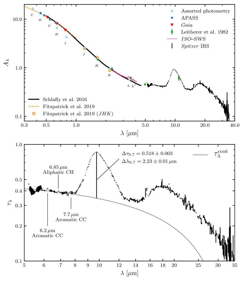
Figure 4: In the top panel, we plot the extinction curve computed from the modeled and observed fluxes (see Table 1). We compare this curve to the Milky Way mean extinction curves derived by Schlafly et al. (2016) (black solid) and Fitzpatrick et al. (2019) (orange dashed). In the bottom panel, we plot the inferred optical depth $\tau_{\lambda}$ from the IRS spectrum. We find $\Delta\tau_{9.7}=0.518$ using the adopted linear continuum (dashed line, Equation 14).

4.1 Model Constraints

After subtracting the best-fit models of the various lines, the continuum flux can be modeled using the formalism described in Section 3.1. To constrain the two free model parameters $\theta_{\star}$ and $\dot{M}$, we consider what is known about the shape of the extinction curve.

Despite the large amount of reddening, the extinction along the sightline toward Cyg OB2-12 appears typical of the diffuse ISM in both the shape of the UV/optical extinction curve and the lack of ice features (Whittet, 2015). Thus, we posit that the extinction law toward Cyg OB2-12 should also agree with recent determinations of the mean Galactic extinction curve at infrared wavelengths.

Employing a sample of 37,000 stars and photometry from PAN-STARRS1, the Two Micron All-Sky Survey (2MASS), and the Wide-field Infrared Survey Explorer (WISE), Schlafly et al. (2016) made a determination of the mean Galactic interstellar extinction curve extending from 5000 Å to 4.5 $\mu$m. This curve is shown in the top panel of Figure 4 for its default parameters of $A_{H}/A_{K}=1.55$ (Indebetouw et al., 2005) and $x=0$ (equivalent to $R_{V}\simeq 3.3$). Recently, Fitzpatrick et al. (2019) derived the mean Milky Way interstellar extinction law from the ultraviolet to the near-infrared using spectrophotometry from the Hubble Space Telescope, archival data from the International Ultraviolet Explorer, and photometry in the $JHK$ bands from 2MASS. We use this extinction law to guide our model fits as well and present it alongside that of Schlafly et al. (2016) in Figure 4.

At far-infrared (FIR) wavelengths, the properties of interstellar dust are well-constrained by observations of dust emission. In particular, Planck observations of dust emission are well-fit by a power law dust opacity $\kappa_{\nu}$, where $\kappa_{\nu}\propto\lambda^{-1.53}$ between 350 $\mu$m and $\sim$3 mm (Planck Collaboration Int. XXII, 2015; Planck Collaboration X, 2016). Since scattering is negligible at these wavelengths, the extinction cross section and thus the optical depth should also scale as $\lambda^{-1.53}$ for $\lambda\gtrsim 350\,\mu$m. We therefore require our model to yield an extinction curve having approximately this behavior longward of the 18 $\mu$m silicate feature.

We can in principle improve further on the connection of MIR extinction to FIR emission. The FIR dust emission is well-fit with a dust temperature of 20 K (Planck Collaboration Int. XXII, 2015), and the dust emission in the Planck 857 GHz (350 $\mu$m) band per $N_{\rm H}$ at high Galactic latitudes has been determined to be $4.3\times 10^{-21}$ MJy sr^-1 cm² (Planck Collaboration Int. XVII, 2014). This implies $\tau_{857}/N_{\rm H}=3.2\times 10^{-26}$ cm². On high-latitude sightlines, $N_{\rm H}/E(B-V)=8.8\times 10^{21}$ cm^-2 mag^-1 (Lenz et al., 2017), and so $\tau_{857}/A_{V}=9.0\times 10^{-5}$ mag^-1 assuming $R_{V}=3.1$. Thus, if the ratio of optical to infrared extinction is constant across the sky, we would expect the sightline toward Cyg OB2-12 to have $\tau_{857}\simeq 9.0\times 10^{-4}$ since $A_{V}\simeq 10$.

Alternatively, $N_{\rm H}$ has been estimated toward Cyg OB2-12 to be $2\times 10^{22}$ cm^-2 by fitting X-ray absorption data (Oskinova et al., 2017). We note that determinations of $N_{\rm H}/E(B-V)$ near the Galactic plane (e.g., Bohlin et al., 1978) are $\sim 50$% lower than those at high Galactic latitudes (e.g., Liszt, 2014; Lenz et al., 2017), suggesting a possible systematic difference in dust to gas ratio. If we assume that the interstellar dust toward Cyg OB2-12 has the same properties as that observed at high Galactic latitudes but is simply 50% more abundant per H atom, then we would estimate that $\tau_{857}\simeq 3.2\times 10^{-26}$ cm${}^{2}\times 2\times 10^{22}$ cm${}^{-2}\times 1.5=9.5\times 10^{-4}$.

Given the concordance between these estimates, we require that our model yield an extinction curve which extrapolates to $\tau\simeq 9\times 10^{-4}$ at 350 $\mu$m. Using the dust emission per H atom measured at other frequencies by Planck Collaboration Int. XVII (2014), we likewise estimate $\tau\simeq 4\times 10^{-4}$ at 550 $\mu$m and $\tau\simeq 2\times 10^{-4}$ at 850 $\mu$m.

4.2 Model Fits

Using the formalism outlined in Section 3.1, we can compute a model flux at every wavelength of interest given values for $\theta_{\star}$ and $\dot{M}$. We obtain the extinction curve by comparing to the observed fluxes listed in Table 1. For all data except from those from Gaia, we do not take into account the instrumental bandpasses, i.e., we assume the observed fluxes are the monochromatic fluxes at the central wavelength. However, the Gaia bandpasses are quite broad and so we consider the bandpasses explicitly. Specifically, we assume that the extinction law across each bandpass is given by the Fitzpatrick et al. (2019) curve and solve for total extinction at the nominal wavelength $\lambda_{0}$. We work in units of photoelectrons per second following the Gaia Data Release 2 Documentation (v1.2; van Leeuwen et al., 2018).

We find that $\theta_{\star}=2.65\times 10^{-9}$ rad and $\dot{M}=2.4\times 10^{-6}\,M_{\odot}$ yr^-1 produce an extinction curve most consistent with the considerations discussed in Section 4.1. The model fluxes for the star and wind are illustrated in Figure 1. The resulting extinction curve is presented in detail in Figure 4, and the extinction $A_{\lambda}$ in each photometric band is listed in Table 1.

Good agreement is obtained with both the Schlafly et al. (2016) and Fitzpatrick et al. (2019) mean extinction laws, with only the historical $R$ and $I$ band measurements being significantly discrepant. Given that this disagreement is not found with the Gaia observations of Cyg OB2-12 over the same wavelength range, this might be due to the $R$ and $I$ bandpasses being significantly different than assumed or, particularly in light of the long time baseline, stellar variability. The minor difference between our derived $A_{V}=9.86$ and other determinations of $A_{V}\simeq 10.2$ (e.g. Humphreys, 1978; Torres-Dodgen et al., 1991; Clark et al., 2012) is not unexpected given our simple model of the stellar emission which, while consistent with more detailed modeling in the infrared, does not capture the complexities at optical and UV wavelengths (Castelli & Kurucz, 2003; Clark et al., 2012).

With these parameters and a distance of 1.75 kpc, Cyg OB2-12 has a luminosity $L_{\star}=1.4\times 10^{6}\,L_{\odot}$. Our adopted $\dot{M}=2.4\times 10^{-6}\,M_{\odot}$ yr^-1 is close to the value $\dot{M}=3\times 10^{-6}\,M_{\odot}\,$yr^-1 estimated by Clark et al. (2012). In our model, the wind and the stellar disk contribute equally at 50 $\mu$m.

While our model and that of Clark et al. (2012) are very similar over the wavelengths covered by the Spitzer IRS observations, the small differences are significant for our purposes. In particular, the Clark et al. (2012) model implies a significantly larger 30 $\mu$m extinction, which is difficult to reconcile with the FIR opacities inferred from dust emission. Likewise, the implied 25–35 $\mu$m extinction would then fall off too slowly compared to the $\sim\lambda^{-1.53}$ behavior expected in the FIR.

Figure 1 presents a number of radio observations of Cyg OB2-2. Clark et al. (2012) assume clumping in the outer wind in order to reproduce the observed radio emission. However, recent detection of variability at 20 cm over only 14 days (Morford et al., 2016) suggests that some other source may be responsible for much of the flux at $\lambda>6$ cm, with the $\sim$400 km s^-1 wind from Cyg OB2-12 accounting for only a fraction of the observed radio emission.

There is an X-ray source coincident with Cyg OB2-12 (Waldron et al., 1998; Oskinova et al., 2017). Oskinova et al. (2017) suggest that the X-ray emission may arise from colliding stellar winds, if the close companion recently discovered by Caballero-Nieves et al. (2014) is an O star with a fast wind. This colliding wind scenario could account for much of the observed radio emission, but should not affect the 5–35 $\mu$m spectrum of interest here (except perhaps for emission lines from species such as [SIV]). Thus, we are unconcerned that our model flux is well below the observed radio emission. High angular resolution observations are needed to clarify the origin of the mm-wave continuum.

4.3 Normalized Extinction Curve

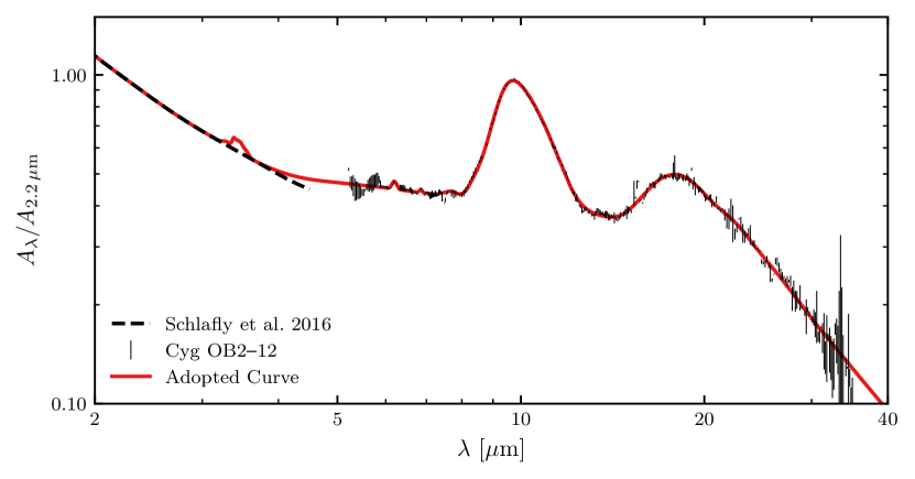
Figure 5: We construct the representative extinction curve presented in this work (red solid) by joining the mean Milky Way extinction curve in the optical and near-IR from Schlafly et al. (2016) (black dashed) with our determination of the total extinction toward Cyg OB2-12 from the Spitzer IRS spectroscopy (black error bars). Extrapolated to FIR wavelengths, the adopted curve is also consistent with dust opacities inferred from Planck observations of dust emission (see Section 4.3). The 3.4 $\mu$m feature is added to the Schlafly et al. (2016) curve following our determination from the ISO-SWS data (see Section 5.3).

Figure 6: Comparison of the adopted extinction law to the Spitzer IRS spectrum of Cyg OB2-12 (black error bars) and the $\tau_{\lambda}$ estimates made from Planck observations of dust emission (shaded region, see Section 4.1). The extent of the shaded region represents varying the dust temperature from 16 to 24 K. The parameterization given in Equation 12 is shown by the dotted line.

With its high signal to noise and spectral resolution, the Spitzer IRS spectrum of Cyg OB2-12 provides perhaps the most detailed characterization of MIR extinction from the diffuse ISM of any current data. We therefore propose using these data to extend determinations of the mean Galactic extinction curve into the MIR and even FIR.

In Figure 5, we plot our Cyg OB2-12 extinction curve normalized to unity at 2.2 $\mu$m, roughly $K$ band, assuming $A_{2.2\,\mu{\rm m}}=0.96$ (see Table 1). We illustrate in red our synthesized curve, which matches onto the Schlafly et al. (2016) curve at short wavelengths and interpolates smoothly through the Spitzer IRS data in the MIR. Based on broadband photometry, the Schlafly et al. (2016) extinction law does not include spectral features, and so we employ the ISO-SWS spectrum to characterize this spectroscopic feature near 3.4 $\mu$m (see Section 5.3 below).

The extinction at $\lambda\gtrsim 20\,\mu$m is well-fit by

$$A_{\lambda}/A_{2.2\,\mu{\rm m}}=2.76\times 10^{-4}\left(\frac{850\,\mu{\rm m}}{\lambda}\right)^{1.52+\Delta\beta\left(\lambda\right)}~{}~{}~{},$$ (12)

where

$$\Delta\beta\left(\lambda\right)=0.1\ln\left[\frac{2\,{\rm mm}}{{\rm min}\left(\lambda,2\,{\rm mm}\right)}\right]$$ (13)

and $\ln$ is the natural logarithm. For Cyg OB2-12, this yields $\tau=0.41$ at 20 $\mu$m, $1.1\times 10^{-3}$ at 350 $\mu$m, and $2.4\times 10^{-4}$ at 850 $\mu$m, in agreement with Figure 4 and the FIR estimates based on Planck data discussed in Section 4.1. Further, the polarized dust intensity measured by Planck is well-described with an opacity scaling as $\lambda^{-1.53\pm 0.02}$ from 850 $\mu$m to 7.5 mm (Planck Collaboration XI, 2018), suggesting that Equation 12 is an appropriate estimate well into the microwave. The extrapolation to the Planck frequencies is illustrated in Figure 6, where the shaded band shows the effect of varying the assumed dust temperature between 16 and 24 K.

To the extent that the sightline toward Cyg OB2-12 typifies extinction from the diffuse ISM, our synthesized extinction curve extends the determinations of the mean Galactic extinction from $\sim 4\,\mu$m through the FIR. We will make this extinction curve available in tabular form following publication.

5 Extinction Features Toward Cyg OB2-12

The high signal to noise and spectral resolution of the ISO-SWS and Spitzer IRS data enable identification of a number of spectroscopic extinction features that have been identified with specific materials. In this section, we identify and characterize a number of these features.

Table 4: Cyg OB2-12 Extinction Features

Silicate Features
$\lambda_{0}$	$\Delta\tau$	$\Delta\lambda$	$\Delta\lambda^{-1}$	$\int d\lambda^{-1}\Delta\tau$
$[\mu$m]		[$\mu$m]	[cm-1]	[cm-1]
9.7	$0.518\pm 0.003$	$2.23\pm 0.01$	$240\pm 1$	$119\pm 2$
18	0.22	5.7	172	68
Carbonaceous Features
$\lambda_{0}$	$\Delta\tau$	$\Delta\lambda$	$\Delta\lambda^{-1}$	$\int d\lambda^{-1}\Delta\tau$
$[\mu$m]		[$\mu$m]	[cm-1]	[cm-1]
3.3	$0.014\pm 0.005$	0.10	96	1.41
3.4	$0.044\pm 0.005$	0.18	156	6.61
6.2	$0.022\pm 0.001$	$0.127\pm 0.003$	$32.9\pm 0.8$	$0.78\pm 0.03$
6.85	$0.009\pm 0.001$	$0.086\pm 0.009$	$18\pm 2$	$0.21\pm 0.03$
7.7	$0.017\pm 0.002$	$0.54\pm 0.08$	$91\pm 13$	$2.5\pm 0.4$

Note. — Reported uncertainties on the 6.2, 6.85, 7.7, and 9.7 $\mu$m feature parameters are statistical only. The properties of the 3.3 and 3.4 $\mu$m features are derived from the best fit Gaussian decomposition presented in Figure 7 and Table 5 with quoted uncertainties estimated from alternate fits of the underlying continuum. Parameters of the 18 $\mu$m feature are quoted based on the fiducial continuum model (Equation 14), which is relatively unconstrained at these wavelengths.

5.1 Continuum Extinction

Before analyzing the profiles of the MIR dust extinction features, it is first necessary to determine the underlying continuum. Our estimate of the continuum is based on the 6–8 $\mu$m IRS spectrum between the dust extinction features. At shorter wavelengths, the IRS data become noisy, and at longer wavelengths the extinction is dominated by the silicate features. In Section 5.3, we demonstrate that the simple linear function

$$\tau_{\lambda}^{\rm cont}=-0.0155\left(\frac{\lambda}{\mu{\rm m}}\right)+0.494$$ (14)

describes the continuum extinction over the 6–8 $\mu$m range and extrapolates well to the extinction curve at shorter wavelengths (see Figures 4 and 8). The extinction in the dust features $\Delta\tau_{\lambda}$ is then determined by

$$\Delta\tau_{\lambda}\equiv\tau_{\lambda}-\tau_{\lambda}^{\rm cont}~{}~{}~{}.$$ (15)

5.2 Silicate Features

As seen in Figure 4, the most prominent MIR dust extinction features toward Cyg OB2-12 are the 9.7 and 18 $\mu$m silicate features. To determine the feature profiles, we model the underlying continuum with Equation 14. While it is probably reasonable to extrapolate Equation 14 to 9.7 $\mu$m, the assumption of a linear continuum becomes increasingly unreliable at longer wavelengths, with the adopted function eventually going to zero at 31.9 $\mu$m.

Including the uncertainty in the underlying continuum from the fits in Section 5.3, we find that $\Delta\tau_{9.7}=0.518\pm 0.003$. The feature has a FWHM of $2.23\pm 0.01$ $\mu$m and an integrated area of $119\pm 2$ cm^-1. We list these values in Table 4. Assuming $A_{V}\simeq 10$, this implies $A_{V}/\Delta\tau_{9.7}=19.3$, within the range observed on other sightlines (Draine, 2003).

Extrapolating Equation 14 to 18 $\mu$m, we find that $\tau_{18}^{\rm cont}=0.22$ and $\Delta\tau_{18}=0.22\pm 0.01$ with $\Delta\tau_{18}/\Delta\tau_{9.7}\simeq 0.42$. Based on the short wavelength side of the feature only, we estimate a FWHM of 5.7 $\mu$m, extending roughly from 15.6 to 21.2 $\mu$m and peaking at 18.4 $\mu$m. However, these quantities depend sensitively on the underlying continuum, which is relatively unconstrained particularly on the long wavelength side.

The detailed shapes of the silicate features provide constraints on the precise composition of interstellar silicate materials, such as the O:Si:Mg:Fe ratios. Fogerty et al. (2016) performed a detailed comparison of these data to laboratory materials, finding evidence for a silicate stoichiometry intermediate between olivine and pyroxene. While we do not perform additional analysis on the nature of the silicate material itself, we note that evident subfeatures in the profiles in Figure 4 that have persisted even after subtracting line emission from the stellar wind may provide additional clues to the detailed composition of interstellar silicates and should be further pursued. Of particular note is an apparent feature at $\sim 13.8\,\mu$m in the IRS data (see Figures 2 and 4), though it is unclear whether this is astrophysical rather than instrumental in origin.

5.3 Carbonaceous Features

A close inspection of the Cyg OB2-12 extinction curve reveals absorption features in addition to the prominent silicate features, as indicated in Figure 4. The ISO-SWS spectrum allows detailed characterization of the prominent 3.4 $\mu$m feature associated with aliphatic hydrocarbons. The features in the IRS spectrum at 6.2 and 7.7 $\mu$m are recognizable as PAH features, though seen in absorption rather than emission. In addition, we detect the 6.85 $\mu$m feature arising from aliphatic hydrocarbons. We now explore each of these features in greater detail.

5.3.1 The 3.4 $\mu$m Complex

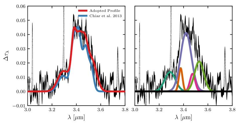
Figure 7: Determination of the 3.4 $\mu$m feature profile from the ISO-SWS spectrum (black). An absorption feature at 3.3 $\mu$m attributed to aromatic carbon is also present. In the left panel, we present the Gaussian decomposition of the feature profile in red, while the right panel shows each Gaussian component. The corresponding fit parameters listed in Table 5. The 3.4 $\mu$m feature profile derived on sightlines toward the Quintuplet Cluster (Chiar et al., 2013) is shown in the right panel in blue, demonstrating excellent agreement. The prominent absorption lines at 3.039, 3.296, and 3.740 $\mu$m are Pf $\epsilon$, $\delta$, and $\gamma$, respectively.

Table 5: Gaussian Decomposition of the 3.4 $\mu$m Feature

$\lambda_{0}$	$\Delta\tau_{\lambda_{0}}$	$\Delta\lambda$	$\Delta\lambda^{-1}$	$\int d\lambda^{-1}\Delta\tau$
$[\mu$m]		[$\mu$m]	[cm-1]	[cm-1]
3.289	0.014	0.10	96	1.41
3.376	0.016	0.04	31	0.55
3.420	0.041	0.10	89	3.91
3.474	0.012	0.05	41	0.55
3.528	0.021	0.09	71	1.61

By far the most prominent extinction feature visible in the ISO-SWS spectrum is the extinction feature at 3.4 $\mu$m (see Figure 4) arising from the C–H stretching mode in aliphatic hydrocarbons. Prior determinations of the strength of this feature toward Cyg OB2-12 have been made with UKIRT (Adamson et al., 1990) and ISO (Whittet et al., 1997), which found $\Delta\tau_{3.4}=0.03\pm 0.01$ and $0.04\pm 0.01$, respectively.

We present our determination of the 3.4 $\mu$m feature profile in Figure 7. The depth of the feature at 3.4 $\mu$m depends on the details of the assumed continuum. We estimate $\Delta\tau_{3.4}=0.044\pm 0.005$, in good agreement with the $\Delta\tau_{3.4}$ derived by Whittet et al. (1997) but somewhat higher than that of Adamson et al. (1990), whose determination has $\Delta\tau=0$ near 3.3 $\mu$m. We estimate a feature FWHM of 0.18 $\mu$m.

Using ISO-SWS measurements toward the Quintuplet Cluster, Chiar et al. (2013) derived a Gaussian decomposition of the extinction near 3.4 $\mu$m using five distinct components. We compare that profile to the observed extinction toward Cyg OB2-12 in Figure 7, where we have scaled it to $\Delta\tau_{3.4}=0.044$. The overall agreement is very good. In particular, both the Chiar et al. (2013) profile and the Cyg OB2-12 spectrum suggest a feature at 3.3 $\mu$m expected from aromatic hydrocarbons with strength $\Delta\tau_{3.3}\simeq 0.01$.

The Chiar et al. (2013) profile departs from the Cyg OB2-12 spectrum in two principal ways. First, it underestimates the absorption in the vicinity of 3.47 $\mu$m. This appears to be a genuine difference in the feature profiles between Cyg OB2-12 and the Galactic Center. Second, it slightly underestimates the extinction in the red wing of the feature, $\lambda\gtrsim 3.55\,\mu$m. However, this is also true of the Quintuplet Cluster spectrum, and thus appears to be a shortcoming of the Gaussian fit.

Following Chiar et al. (2013), we fit the 3.4 $\mu$m feature with the sum of five Gaussian components

$$\Delta\tau_{\lambda}=\sum_{j=1}^{5}\Delta\tau_{j}{\rm exp}\left[-\left(4\ln 2\right)\left(\frac{\lambda-\lambda_{0,j}}{\Delta\lambda_{j}}\right)^{2}\right]~{}~{}~{},$$ (16)

where for each component $j$, $\lambda_{0,j}$ is the central wavelength, $\Delta\lambda_{j}$ is the FWHM, and $\Delta\tau_{j}$ is the optical depth at $\lambda_{0}$. Note that $\Delta\lambda$ is related to $\Delta\lambda^{-1}$ via

$$\Delta\lambda^{-1}=\frac{1}{\lambda_{0}-\Delta\lambda/2}-\frac{1}{\lambda_{0}+\Delta\lambda/2}~{}~{}~{}.$$ (17)

The best fit parameters of our Gaussian decomposition are listed in Table 5, and the resulting profile is presented in Figure 7. We have followed Chiar et al. (2013) in including components at 3.289, 3.376, 3.420, and 3.474 $\mu$m, which they attribute to aromatic CH, the CH₃ asymmetric mode, the CH₂ asymmetric mode, and the CH₃ symmetric mode, respectively. While they include a 3.520 $\mu$m component attributed to the CH₂ symmetric mode, we shift this component to 3.528 $\mu$m to better fit the red wing of the feature.

The 3.3 $\mu$m aromatic feature is best fit with $\Delta\tau_{3.3}=0.014\pm 0.005$, where the uncertainty is estimated from different treatments of the continuum. With the determination presented in Figure 7, the feature has roughly the same strength relative to the 3.4 $\mu$m feature as towards the Galactic Center.

If the 3.3 $\mu$m feature is arising from PAH absorption, we can estimate the PAH abundance required to reproduce the observed strength. Using the absorption cross sections proposed by Draine & Li (2007), the absorption due to PAHs $\Delta\tau_{\lambda}^{\rm PAH}$ is given by

$$\Delta\tau_{\lambda}^{\rm PAH}=N_{\rm H}A_{\rm C}^{\rm PAH}\sum_{j}\left(\frac{2}{\pi}\right)\frac{\gamma_{j}\lambda_{j}\sigma_{j}}{\left(\lambda/\lambda_{j}-\lambda_{j}/\lambda\right)^{2}+\gamma_{j}^{2}}~{}~{}~{},$$ (18)

where for each component $j$, $\lambda_{j}$ is the peak wavelength, $\gamma_{j}\lambda_{j}$ is the FWHM, $\sigma_{j}$ is the integrated strength of the feature, and $A_{\rm C}^{\rm PAH}$ is the number of C atoms per H in PAHs. From their Table 1, the feature peaking at 3.300 $\mu$m has $\gamma_{j}=0.012$ and $\sigma_{j}=3.95\times 10^{-18}$ cm per CH in neutral PAHs and $0.89\times 10^{-18}$ cm per CH in ionized PAHs.

For a column density of $N_{\rm H}=2\times 10^{22}\,$cm^-2 (Oskinova et al., 2017), the observed integrated area is compatible with $\sim 18$ ppm of CH in neutral PAHs, or 81 ppm of CH in ionized PAHs. The Draine & Li (2007) model (with 60 ppm C in PAHs) has only 8 ppm CH in neutral PAHs and $\sim 8$ ppm CH in ionized PAHs, thus accounting for less than 50% of the observed integrated absorption in the 3.3 $\mu$m feature.

As noted by Chiar et al. (2013), the Quintuplet Cluster 3.3 $\mu$m profile is significantly wider ($\Delta\lambda\simeq 0.09\,\mu$m, $\Delta\lambda^{-1}\simeq 80$ cm^-1) than observed in emission ($\Delta\lambda\simeq 0.04\,\mu$m, $\Delta\lambda^{-1}\simeq 30$ cm^-1; Tokunaga et al., 1991; Joblin et al., 1996; Li & Draine, 2001). The 3.3 $\mu$m feature toward Cyg OB2-12 appears equally broad as that observed toward the Galactic Center. Only small free-flying PAHs with $\lesssim 200$ C atoms that have been excited by single photon heating become hot enough to radiate at 3.3 $\mu$m (see Draine & Li, 2007, Figure 7). In contrast, the 3.3 $\mu$m absorption feature arises from all grains. It is thus conceivable that additional PAH material is present in large grains and accounts for the observed strength of the 3.3 $\mu$m absorption feature. Likewise, the greater diversity of material seen in absorption may explain the observed breadth relative to the emission feature. Absorption spectroscopy of the 3.3 $\mu$m feature on more sightlines would be useful to establish whether a relatively broad extinction feature is indeed typical.

The 3.47 $\mu$m feature is thought to arise from H atoms attached to diamond-like $sp^{3}$ bonded C (Allamandola et al., 1992). From detection of this feature in a sample of young stellar objects, Brooke et al. (1996) found that the feature was much better correlated with the strength of the H₂O ice features rather than the silicate features, and thus that the feature likely arises in dense molecular gas rather than the diffuse ISM. The detection of the feature toward the Galactic Center by Chiar et al. (2013) is consistent with this hypothesis. Thus, it is surprising that the ice-free sightline toward Cyg OB2-12 has stronger relative absorption near 3.47 $\mu$m than the Galactic Center sightline. If indeed this absorption is due to diamond-like carbon, then this may be a generic component of dust in the diffuse ISM. However, as illustrated by the Gaussian decomposition in Figure 7, other features in the vicinity of 3.47 $\mu$m could also account for the enhanced extinction.

Assuming an absorption strength of $2.37\times 10^{-17}$ cm per CH₃ (Chiar et al., 2013) and an integrated area of 0.55 cm^-1 (see Table 5), this implies 1.2 ppm of CH₃ in diamond-like form. If the 3.47 $\mu$m feature dominates the 3.47 $\mu$m absorption, unlike in our Gaussian decomposition, then this could be a factor of a few higher.

5.3.2 The 6.2, 6.85, and 7.7 $\mu$m Features

Figure 8: We perform a simultaneous fit to the 6.2, 6.85. and 7.7 $\mu$m features observed in the Spitzer IRS data as well as the underlying continuum. The parameters of the fit Gaussian profiles are listed in Table 4.

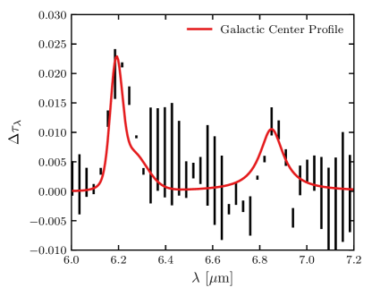
Figure 9: In red we plot the carbonaceous feature profiles derived by Chiar et al. (2000) and Chiar et al. (2013) based on observations toward the Galactic Center and rescaled to match the observed strength of the 3.4 $\mu$m feature toward Cyg OB2-12. We compare this to the Spitzer IRS data in black, finding that both the 6.2 and 6.85 $\mu$m features have approximately the same strength relative to the 3.4 $\mu$m feature as toward the Galactic Center.

The extinction curve derived from the low-resolution IRS spectrum has broad extinction features between 6 and 8 $\mu$m (see Figure 4). We attribute these to the 6.2 and 7.7 $\mu$m aromatic C features and the 6.85 $\mu$m aliphatic C feature.

To quantify the observed strengths of the detected carbonaceous features, we adopt a Gaussian profile for each of the three features and fit the strengths and FWHMs simultaneously with the slope and intercept of a linear continuum over the wavelength range 5.8–8 $\mu$m. No attempt is made to fit subfeatures given the limited wavelength resolution of the data. Thus, the adopted parametric model is

$$\tau_{\lambda}=b+m\lambda+\sum_{j=1}^{3}\Delta\tau_{j}^{\rm exp}\left[-\left(4\ln 2\right)\left(\frac{\lambda-\lambda_{0,j}}{\Delta\lambda_{j}}\right)^{2}\right]$$ (19)

where $m$ and $b$ are the slope and intercept of the linear continuum (Equation 14), respectively, and for each component $j$, $\lambda_{0,j}$ is the central wavelength, $\Delta\tau_{j}$ is the optical depth at $\lambda_{0,j}$, and $\Delta\lambda_{j}$ is FWHM. We note that in this formulation, the data model is required to account for all of the 8 $\mu$m extinction whereas the 9.7 $\mu$m silicate feature must also be contributing at least somewhat at this wavelength. This may result in the depth of the 7.7 $\mu$m feature and/or the continuum to be slightly overestimated.

We perform this fit using the emcee Markov Chain Monte Carlo software (Foreman-Mackey et al., 2013). We adopt flat, uninformative priors on all parameters. Because of the imperfect subtraction of the Pf $\alpha$ line (see Section 3.2), we exclude the data from 7.4 to 7.55 $\mu$m.

The results of the fit are presented in Table 4, where the quoted uncertainties have been marginalized over all fit parameters but do not include any uncertainties inherent in the overall flux model employed to derive $\tau_{\lambda}$ (see Section 3), which are difficult to quantify. The best fit profiles of each of the three features are illustrated in Figure 8.

This model provides an excellent fit to the data over this wavelength range despite its simplicity. There is some suggestion that the Gaussian profile is overpredicting the extinction on the short wavelength side of the 6.2 $\mu$m feature, and the continuum appears high relative to a few points near 6.7 $\mu$m, but there is no clear evidence of unmodeled features at the sensitivity of the data.

As with the 3.4 $\mu$m feature, we can compare the feature profiles observed toward Cyg OB2-12 to those toward the Quintuplet Cluster (Chiar et al., 2013). In that study, the 6.2 $\mu$m feature was divided into two distinct components. The broader of these two components was attributed to the aromatic C–C mode ($\lambda_{0}=6.25\,\mu$m, $\Delta\lambda^{-1}=40\,$cm^-1) while the narrower component was attributed to the aliphatic C–C mode ($\lambda_{0}=6.19\,\mu$m, $\Delta\lambda^{-1}=15\,$cm^-1). The feature optical depths relative to the 3.4 $\mu$m feature were found to be 0.40 and 0.15, respectively. In Figure 9, we scale the Quintuplet Cluster profile to the $\Delta\tau_{3.4}=0.044$ observed toward Cyg OB2-12. The agreement is excellent, suggesting that the 3.4 and 6.2 $\mu$m features have comparable strengths in both dense and diffuse gas.

The 6.85 $\mu$m feature has been observed on the sightline toward the Galactic Center with both the Kuiper Airborne Observatory (Tielens et al., 1996) and ISO (Chiar et al., 2000) and is attributed to CH deformation modes in aliphatic carbon. The 6.85 $\mu$m feature toward Sgr A* is well-fit by a Lorentzian with $\Delta\tau_{6.85}=0.05\pm 0.01$ and $\Delta\lambda^{-1}=26\,$cm^-1 (Chiar et al., 2000). The sightline toward Sgr A* has $\tau_{3.4}=0.21\pm 0.01$ (Chiar et al., 2000), and so $\Delta\tau_{6.85}/\Delta\tau_{3.4}=0.24\pm 0.05$. In Figure 9, we scale this profile to the $\Delta\tau_{3.4}=0.044$ observed toward Cyg OB2-12. As with the 6.2 $\mu$m feature, the predicted strength matches the Cyg OB2-12 observations. Thus, the 6.85 $\mu$m feature appears to be a generic component of dust extinction even in the diffuse ISM.

Unlike the 3.3 $\mu$m feature which is dominated by neutral PAHs, the 6.2 and 7.7 $\mu$m features arise mostly from ionized grains. Using the adopted band strengths from Draine & Li (2007) and a column density of $2\times 10^{22}$ cm^-2 (Oskinova et al., 2017), we find that a 6.2 $\mu$m optical depth of 0.022 can be produced by 35 ppm of C in ionized PAHs. Likewise, a 7.7 $\mu$m optical depth of 0.017 can be produced by 28 ppm of C in ionized PAHs. This is well within the $\sim 60\,$ppm of C thought to be in PAHs. The slight difference in the predicted abundances is within the systematic uncertainties of the model fit, particularly the determination of the 7.7 $\mu$m feature strength. The observed extinction is therefore consistent with arising from PAH absorption and may constrain the amount of PAH material present in larger grains.

To our knowledge, this is the first identification of the 7.7 $\mu$m aromatic feature in absorption. The ISO-SWS spectrum of Sgr A* has a clear feature in the vicinity of 7.7 $\mu$m which Chiar et al. (2000) identify with methane ice. Given that the observed depth of the feature is only slightly less than the 6.2 $\mu$m feature on the same sightline ($0.02$ vs. $0.05\pm 0.01$), it is possible that PAH absorption rather than CH₄ ice is responsible. Given the absence of other ice features, it is unlikely that the 7.7 $\mu$m feature observed toward Cyg OB2-12 arises from solid methane, and we therefore identify it as PAH absorption.

In principle, PAH absorption features at longer wavelengths are present in the Spitzer IRS spectrum. However, owing to the relative weakness of these features and the prominence of the silicate features, we find no evidence of other PAH absorption features. For instance, the Draine & Li (2007) PAH absorption profile predicts $\Delta\tau\lesssim 0.009$ in the vicinity of 8.6 $\mu$m, which would not be discernible in these data particularly given the contribution from the 9.7 $\mu$m feature at this wavelength.

5.3.3 The 7.25 $\mu$m Aliphatic Hydrocarbon Feature

An absorption feature at 7.25 $\mu$m associated with CH₃ symmetric deformation modes has been found toward Sgr A* (Chiar et al., 2000), Seyfert 2 nuclei (Dartois et al., 2004), and luminous infrared galaxies (Dartois & Muñoz-Caro, 2007) at roughly half the strength of the 6.85 $\mu$m feature. As illustrated in Figure 8, the IRS data have no suggestion of a feature at this wavelength. To test this in detail, we redo our simultaneous fit of the 6.2, 6.85, and 7.7 $\mu$m features and linear continuum with the addition of a fourth feature at 7.25 $\mu$m having fixed $\Delta\lambda=0.10$ $\mu$m, consistent with the Sgr A* sightline (Chiar et al., 2000).

We find $\Delta\tau_{7.25}=-0.007\pm 0.010$ with an upper limit of $\Delta\tau_{7.25}<0.007$ at 95% confidence. The inclusion of this feature has little effect on the best fit profiles of the other features, although a large $\Delta\tau_{7.25}$ would require alteration of the 7.7 $\mu$m feature profile. Thus, while disfavored, an absorption feature at 7.25 $\mu$m subdominant to the 6.85 $\mu$m feature ($\Delta\tau_{6.85}=0.009\pm 0.001$) cannot be completely ruled out.

5.3.4 The 11.53 $\mu$m Graphite Feature

Graphite has long been a candidate constituent of interstellar dust for its ability to produce an extinction feature consistent with the 2175 Å bump (Stecher & Donn, 1965). Draine (1984) and Draine (2016) discussed an out of plane lattice resonance in polycrystalline graphite at 11.53 $\mu$m. The expected 0.014 $\mu$m FWHM of this feature is well-matched to the resolution of the high-resolution IRS spectrum, but no evidence of enhanced absorption is present at this wavelength, as shown in Figure 2.

The most pronounced feature in this region of the spectrum is the 11.537 $\mu$m 15–9 hydrogen recombination line. In order to constrain the strength of a possible graphite feature, over the wavelength range 11.43–11.63 $\mu$m we model simultaneously the contribution of the 15–9 line to the total flux, a linear continuum contribution to $\tau_{\lambda}$, and the graphite feature at fixed $\lambda_{0}=11.53\,\mu$m and FHWM 0.014 $\mu$m. We find that the graphite optical depth $\Delta\tau_{11.53}<0.03$ at 95% confidence. Assuming an opacity $\Delta\kappa=470\,$cm² g^-1 (Draine, 2016), this implies $<160$ ppm of C in graphite. Unfortunately, the weakness of the feature and the presence of the recombination line prevent more stringent constraints.

6 Discussion

The heavily reddened sightline toward Cyg OB-12 is ideal for studying MIR extinction from dust in the diffuse ISM, and the ISO-SWS and Spitzer IRS spectra provide high-sensitivity characterization of both the spectroscopic extinction features in this wavelength range as well as the underlying continuum. Thus, the MIR extinction curve constructed in this work provides a new benchmark for models of interstellar dust.

The widely-used “astrosilicate” proposed by Draine & Lee (1984) included a 9.7 $\mu$m silicate feature based on observations of dust emission in the Trapezium region (Forrest et al., 1975). However, the Trapezium profile FWHM $\simeq 3.45\,\mu$m is significantly broader than Cyg OB2-12 profile derived in this work (FWHM = $2.23\pm 0.01\,\mu$m) and elsewhere (Roche & Aitken, 1984; Bowey et al., 1998), as well as other sightlines that probe the diffuse ISM (van Breemen et al., 2011). Thus, for use on diffuse sightlines, the astrosilicate dielectric function should be revised to accord with the Cyg OB2-12 profile.

While the silicate and PAH features were accounted for in the astrosilicate + graphite + PAH modeling paradigm of Draine & Li (2007), the features from aliphatic hydrocarbons at 3.4 and 6.85 $\mu$m were not. Observations of the Cyg OB2-12 sightline provide a detailed characterization of the feature profiles as well as their strengths relative to both the continuum extinction and the other spectroscopic features. These too should be incorporated in models of dust in the diffuse ISM.

Earlier studies of MIR extinction (e.g., Bertoldi et al., 1999; Rosenthal et al., 2000; Hennebelle et al., 2001) suggested a pronounced minimum near 7 $\mu$m, but the extinction curve found in this work is relatively flat in the 4–8 $\mu$m wavelength range, consistent with recent determinations on other sightlines (e.g., Lutz et al., 1996; Lutz, 1999; Jiang et al., 2003; Indebetouw et al., 2005; Chapman et al., 2009; Wang et al., 2013; Xue et al., 2016). In light of this emerging consensus on the behavior of the Galactic extinction curve at these wavelengths, dust models require significant revision. Wang et al. (2015) suggest, for instance, that the additional absorption required could be produced by $\mu$m-sized graphite grains.

We note that the ability to measure PAH absorption on this sightline is particularly valuable since, unlike emission, absorption does not depend on the details of grain heating. Thus, the PAH optical properties are more directly accessed. High resolution followup of these features and deep searches for the longer wavelength features can test models in detail, including ionization fractions and the relative strengths of the various vibrational modes. Such a search should be possible with the Mid-Infrared Instrument on the James Webb Space Telescope.

The most uncertain aspect of the MIR emission from Cyg OB2-12 is the contribution from the stellar wind. In particular, it remains unclear how much of the observed radio emission is the result of the collision of the Cyg OB2-12 wind with that of its nearby companion. Very high angular resolution characterization of the wind morphology, finer than the 60 mas separation between the stars (Caballero-Nieves et al., 2014), would be immensely valuable in understanding the origin of the radio emission and its connection to the MIR emission.

7 Conclusions

The principal conclusions of this work are as follows:

• We develop a model for the MIR emission from Cyg OB2-12 and its stellar wind to derive the total extinction on this sightline from ISO-SWS and Spitzer IRS spectroscopy.

• We identify and characterize more than sixty spectral lines, many of which are H recombination lines seen in both emission and absorption, which may help constrain models of the stellar wind.

• We determine the 3.4 $\mu$m feature profile on this sightline, finding overall close agreement with the feature profile toward the Galactic Center. The extinction in the vicinity of 3.47 $\mu$m is enhanced relative to the Galactic Center sightline, which may point to the presence of diamond-like carbon in the diffuse ISM.

• We find evidence for the 3.3 $\mu$m aromatic hydrocarbon feature in extinction. The feature has a significantly broader profile than is typically seen in emission, in agreement with observations of this feature toward the Galactic Center (Chiar et al., 2013).

• We robustly detect extinction features at 6.2, 6.85, and 7.7 $\mu$m associated with carbonaceous grain materials with relative strengths similar to those on the sightline toward the Galactic Center. The 6.2 and 7.7 $\mu$m feature strengths are compatible with expectations from PAH absorption. To our knowledge, this is the first identification and characterization of the 7.7 $\mu$m aromatic feature in absorption.

• Synthesizing our derived Cyg OB2-12 extinction curve with the mean interstellar extinction curve of Schlafly et al. (2016), we present a representative extinction curve of the diffuse ISM extending through the MIR. We demonstrate that extension of this curve into the FIR is fully compatible with dust opacities inferred from measurements of FIR emission.

References

- Adamson et al. (1990) Adamson, A. J., Whittet, D. C. B., & Duley, W. W. 1990, MNRAS, 243, 400
- Allamandola et al. (1992) Allamandola, L. J., Sandford, S. A., Tielens, A. G. G. M., & Herbst, T. M. 1992, ApJ, 399, 134
- Allamandola et al. (1985) Allamandola, L. J., Tielens, A. G. G. M., & Barker, J. R. 1985, ApJ, 290, L25
- Ardila et al. (2010) Ardila, D. R., Van Dyk, S. D., Makowiecki, W., et al. 2010, ApJS, 191, 301
- Astropy Collaboration et al. (2013) Astropy Collaboration, Robitaille, T. P., Tollerud, E. J., et al. 2013, A&A, 558, A33
- Astropy Collaboration et al. (2018) Astropy Collaboration, Price-Whelan, A. M., Sipőcz, B. M., et al. 2018, AJ, 156, 123
- Berlanas et al. (2019) Berlanas, S. R., Wright, N. J., Herrero, A., Drew, J. E., & Lennon, D. J. 2019, MNRAS, 484, 1838
- Bertoldi et al. (1999) Bertoldi, F., Timmermann, R., Rosenthal, D., Drapatz, S., & Wright, C. M. 1999, A&A, 346, 267
- Bessell et al. (1998) Bessell, M. S., Castelli, F., & Plez, B. 1998, A&A, 333, 231
- Bohlin et al. (1978) Bohlin, R. C., Savage, B. D., & Drake, J. F. 1978, ApJ, 224, 132
- Bowey et al. (1998) Bowey, J. E., Adamson, A. J., & Whittet, D. C. B. 1998, MNRAS, 298, 131
- Brooke et al. (1996) Brooke, T. Y., Sellgren, K., & Smith, R. G. 1996, ApJ, 459, 209
- Caballero-Nieves et al. (2014) Caballero-Nieves, S. M., Nelan, E. P., Gies, D. R., et al. 2014, AJ, 147, 40
- Castelli & Kurucz (2003) Castelli, F., & Kurucz, R. L. 2003, in IAU Symposium, Vol. 210, Modelling of Stellar Atmospheres, ed. N. Piskunov, W. W. Weiss, & D. F. Gray, A20
- Chapman et al. (2009) Chapman, N. L., Mundy, L. G., Lai, S.-P., & Evans, II, N. J. 2009, ApJ, 690, 496
- Chiar et al. (2013) Chiar, J. E., Tielens, A. G. G. M., Adamson, A. J., & Ricca, A. 2013, ApJ, 770, 78
- Chiar et al. (2000) Chiar, J. E., Tielens, A. G. G. M., Whittet, D. C. B., et al. 2000, ApJ, 537, 749
- Clark et al. (2012) Clark, J. S., Najarro, F., Negueruela, I., et al. 2012, A&A, 541, A145
- Contreras et al. (2004) Contreras, M. E., Montes, G., & Wilkin, F. P. 2004, Rev. Mexicana Astron. Astrofis., 40, 53
- Contreras et al. (1996) Contreras, M. E., Rodriguez, L. F., Gomez, Y., & Velazquez, A. 1996, ApJ, 469, 329
- Dartois et al. (2004) Dartois, E., Marco, O., Muñoz-Caro, G. M., et al. 2004, A&A, 423, 549
- Dartois & Muñoz-Caro (2007) Dartois, E., & Muñoz-Caro, G. M. 2007, A&A, 476, 1235
- de Graauw et al. (1996) de Graauw, T., Haser, L. N., Beintema, D. A., et al. 1996, A&A, 315, L49
- Draine (1984) Draine, B. T. 1984, ApJ, 277, L71
- Draine (2003) —. 2003, ARA&A, 41, 241
- Draine (2011) —. 2011, Physics of the Interstellar and Intergalactic Medium (Princeton, NJ: Princeton University Press)
- Draine (2016) —. 2016, ApJ, 831, 109
- Draine & Lee (1984) Draine, B. T., & Lee, H. M. 1984, ApJ, 285, 89
- Draine & Li (2007) Draine, B. T., & Li, A. 2007, ApJ, 657, 810
- Fitzpatrick et al. (2019) Fitzpatrick, E. L., Massa, D., Gordon, K. D., Bohlin, R., & Clayton, G. C. 2019, ApJ, 886, 108
- Fogerty et al. (2016) Fogerty, S., Forrest, W., Watson, D. M., Sargent, B. A., & Koch, I. 2016, ApJ, 830, 71
- Foreman-Mackey et al. (2013) Foreman-Mackey, D., Hogg, D. W., Lang, D., & Goodman, J. 2013, PASP, 125, 306
- Forrest et al. (1975) Forrest, W. J., Gillett, F. C., & Stein, W. A. 1975, ApJ, 195, 423
- Gaia Collaboration et al. (2018) Gaia Collaboration, Brown, A. G. A., Vallenari, A., et al. 2018, A&A, 616, A1
- Harris et al. (1978) Harris, D. H., Woolf, N. J., & Rieke, G. H. 1978, ApJ, 226, 829
- Henden et al. (2016) Henden, A. A., Templeton, M., Terrell, D., et al. 2016, VizieR Online Data Catalog, II/336
- Hennebelle et al. (2001) Hennebelle, P., Pérault, M., Teyssier, D., & Ganesh, S. 2001, A&A, 365, 598
- Houck et al. (2004) Houck, J. R., Roellig, T. L., van Cleve, J., et al. 2004, ApJS, 154, 18
- Humphreys (1978) Humphreys, R. M. 1978, ApJS, 38, 309
- Hunter (2007) Hunter, J. D. 2007, Computing in Science and Engineering, 9, 90
- Indebetouw et al. (2005) Indebetouw, R., Mathis, J. S., Babler, B. L., et al. 2005, ApJ, 619, 931
- Jiang et al. (2003) Jiang, B. W., Omont, A., Ganesh, S., Simon, G., & Schuller, F. 2003, A&A, 400, 903
- Joblin et al. (1996) Joblin, C., Tielens, A. G. G. M., Allamandola, L. J., & Geballe, T. R. 1996, ApJ, 458, 610
- Klochkova & Chentsov (2004) Klochkova, V. G., & Chentsov, E. L. 2004, Astronomy Reports, 48, 1005
- Kochanek et al. (2017) Kochanek, C. S., Shappee, B. J., Stanek, K. Z., et al. 2017, PASP, 129, 104502
- Lebouteiller et al. (2015) Lebouteiller, V., Barry, D. J., Goes, C., et al. 2015, ApJS, 218, 21
- Leger & Puget (1984) Leger, A., & Puget, J. L. 1984, A&A, 137, L5
- Leitherer et al. (1982) Leitherer, C., Hefele, H., Stahl, O., & Wolf, B. 1982, A&A, 108, 102
- Lenz et al. (2017) Lenz, D., Hensley, B. S., & Doré, O. 2017, ApJ, 846, 38
- Li & Draine (2001) Li, A., & Draine, B. T. 2001, ApJ, 554, 778
- Liszt (2014) Liszt, H. 2014, ApJ, 780, 10
- Lutz (1999) Lutz, D. 1999, in ESA Special Publication, Vol. 427, The Universe as Seen by ISO, ed. P. Cox & M. Kessler, 623
- Lutz et al. (1996) Lutz, D., Feuchtgruber, H., Genzel, R., et al. 1996, A&A, 315, L269
- Maryeva et al. (2016) Maryeva, O. V., Chentsov, E. L., Goranskij, V. P., et al. 2016, MNRAS, 458, 491
- Morford et al. (2016) Morford, J. C., Fenech, D. M., Prinja, R. K., Blomme, R., & Yates, J. A. 2016, MNRAS, 463, 763
- Nazé et al. (2019) Nazé, Y., Rauw, G., Czesla, S., Mahy, L., & Campos, F. 2019, A&A, 627, A99
- Oskinova et al. (2017) Oskinova, L. M., Huenemoerder, D. P., Hamann, W. R., et al. 2017, ApJ, 845, 39
- Panagia & Felli (1975) Panagia, N., & Felli, M. 1975, A&A, 39, 1
- Planck Collaboration Int. XVII (2014) Planck Collaboration Int. XVII. 2014, A&A, 566, A55
- Planck Collaboration Int. XXII (2015) Planck Collaboration Int. XXII. 2015, A&A, 576, A107
- Planck Collaboration X (2016) Planck Collaboration X. 2016, A&A, 594, A10
- Planck Collaboration XI (2018) Planck Collaboration XI. 2018, arXiv e-prints, arXiv:1801.04945
- Rauw (2011) Rauw, G. 2011, A&A, 536, A31
- Rieke (1974) Rieke, G. H. 1974, ApJ, 193, L81
- Rieke & Lebofsky (1985) Rieke, G. H., & Lebofsky, M. J. 1985, ApJ, 288, 618
- Roche & Aitken (1984) Roche, P. F., & Aitken, D. K. 1984, MNRAS, 208, 481
- Rosenthal et al. (2000) Rosenthal, D., Bertoldi, F., & Drapatz, S. 2000, A&A, 356, 705
- Schlafly et al. (2016) Schlafly, E. F., Meisner, A. M., Stutz, A. M., et al. 2016, ApJ, 821, 78
- Schutte et al. (1998) Schutte, W. A., van der Hucht, K. A., Whittet, D. C. B., et al. 1998, A&A, 337, 261
- Scuderi et al. (1998) Scuderi, S., Panagia, N., Stanghellini, C., Trigilio, C., & Umana, G. 1998, A&A, 332, 251
- Sloan et al. (2003) Sloan, G. C., Kraemer, K. E., Price, S. D., & Shipman, R. F. 2003, ApJS, 147, 379
- Smith et al. (2007) Smith, J. D. T., Draine, B. T., Dale, D. A., et al. 2007, ApJ, 656, 770
- Stecher & Donn (1965) Stecher, T. P., & Donn, B. 1965, ApJ, 142, 1681
- Tielens et al. (1996) Tielens, A. G. G. M., Wooden, D. H., Allamandola, L. J., Bregman, J., & Witteborn, F. C. 1996, ApJ, 461, 210
- Tokunaga et al. (1991) Tokunaga, A. T., Sellgren, K., Smith, R. G., et al. 1991, ApJ, 380, 452
- Torres-Dodgen et al. (1991) Torres-Dodgen, A. V., Tapia, M., & Carroll, M. 1991, MNRAS, 249, 1
- van Breemen et al. (2011) van Breemen, J. M., Min, M., Chiar, J. E., et al. 2011, A&A, 526, A152
- van der Walt et al. (2011) van der Walt, S., Colbert, S. C., & Varoquaux, G. 2011, Computing in Science and Engineering, 13, 22
- van Leeuwen et al. (2018) van Leeuwen, F., de Bruijne, J. H. J., Arenou, F., et al. 2018, Gaia DR2 documentation, Tech. rep.
- Virtanen et al. (2019) Virtanen, P., Gommers, R., Oliphant, T. E., et al. 2019, arXiv e-prints, arXiv:1907.10121
- Waldron et al. (1998) Waldron, W. L., Corcoran, M. F., Drake, S. A., & Smale, A. P. 1998, ApJS, 118, 217
- Wang et al. (2013) Wang, S., Gao, J., Jiang, B. W., Li, A., & Chen, Y. 2013, ApJ, 773, 30
- Wang et al. (2015) Wang, S., Li, A., & Jiang, B. W. 2015, ApJ, 811, 38
- Whittet (2015) Whittet, D. C. B. 2015, ApJ, 811, 110
- Whittet et al. (1997) Whittet, D. C. B., Boogert, A. C. A., Gerakines, P. A., et al. 1997, ApJ, 490, 729
- Wisniewski et al. (1967) Wisniewski, W. Z., Wing, R. F., Spinrad, H., & Johnson, H. L. 1967, ApJ, 148, L29
- Woolf & Ney (1969) Woolf, N. J., & Ney, E. P. 1969, ApJ, 155, L181
- Wright & Barlow (1975) Wright, A. E., & Barlow, M. J. 1975, MNRAS, 170, 41
- Xue et al. (2016) Xue, M., Jiang, B. W., Gao, J., et al. 2016, ApJS, 224, 23