On charm-mass dependent NNLO corrections to $\mathcal{B}(\bar{B}\rightarrow X_{s}\gamma)$

Abstract:

The inclusive radiative decay of the $B$ meson is known to provide strong constraints on many popular extensions of the Standard Model. Such constraints crucially depend on precision of the Standard Model predictions. One of the main contributions to the theoretical uncertainty is due to certain Next-to-Next-to-Leading Order QCD corrections whose values at the physical charm quark mass $m_{c}$ have been estimated using interpolation between the $m_{c}=0$ and $m_{c}\gg m_{b}$ limits. A direct determination of such corrections at the physical value of $m_{c}$ requires calculating hundreds of two-scale four-loop propagator diagrams with unitarity cuts. Applying the integration-by-parts method, we express the corrections in terms of master integrals. Asymptotic expansions of these integrals at $m_{c}\gg m_{b}$ serve as boundary conditions for differential equations in $z=m_{c}^{2}/m_{b}^{2}$ that are being numerically solved. Here, we present our final results for the diagrams involving massless and massive fermion loops on the gluon lines. For the two-body cuts, we confirm the analytical expressions and/or numerical fits that are already present in the literature. In the four-body case, we make the correction complete by including several diagrams that have previously been only estimated using interpolation in $m_{c}$. We also report the status of the ongoing calculation of the remaining diagrams where no closed fermion loops on the gluon lines are present.

1 Introduction

The flavour-changing neutral current transition $\bar{B}\rightarrow X_{s}\gamma$ proceeds via one-loop electroweak penguin diagrams at the leading order in the Standard Model (SM). It provides important constraints on parameter spaces of many popular Beyond-SM (BSM) theories. The current SM prediction for the CP- and isospin-averaged branching ratio with $E_{\gamma}>E_{0}=1.6\,$GeV has recently been updated [1]. It reads ${\mathcal{B}}_{s\gamma}^{\rm SM}=(3.40\pm 0.17)\times 10^{-4}$, which should be compared to the previous (2015) value of ${\mathcal{B}}_{s\gamma}^{\rm SM}=(3.36\pm 0.23)\times 10^{-4}$ in Refs. [4, 5]. Both values agree very well with the experimental world average ${\mathcal{B}}_{s\gamma}^{\rm exp}=(3.32\pm 0.15)\times 10^{-4}$ [6] that has been obtained from the results of CLEO [7], Babar [8, 9, 10] and Belle [11, 12], with extrapolation in $E_{0}$ down to $1.6\,$GeV. Constraints on BSM physics strongly depend on how precisely the SM prediction is determined. For instance, with the current precision, the resulting $95\%$ C.L. bound on the charged Higgs boson mass in the Two-Higgs-Doublet Model II calculated as in Ref. [13] is now in the vicinity of $800\,$GeV.

The present SM prediction uncertainty ($\pm 5\%$) has been determined by combining (in quadrature) uncertainties of three different origins: $(i)$ parametric $(\pm 2.5\%$, including non-perturbative effects), $(ii)$ higher-order perturbative $(\pm 3\%)$, and $(iii)$ interpolation in the charm quark mass that is used to estimate some of the $\mathcal{O}(\alpha_{\mathrm{s}}^{2})$ corrections $(\pm 3\%)$ [5]. On the experimental side, the future Belle II measurements are expected to eventually reduce the world average uncertainty from the current $\pm 4.5\%$ to around $\pm 2.6\%$ [14, 15]. Thus, the SM prediction accuracy must be further improved to match the experimental precision.

Here, we focus on contributions that are necessary to remove the uncertainty related to the interpolation in $m_{c}$. To specify our object of interest, we begin with the perturbative rate of weak radiative $b$-quark decay

$$\Gamma(b\rightarrow X^{\rm partonic}_{s}\gamma)=\frac{G_{F}^{2}m^{5}_{b,pole}\alpha_{\mathrm{e}m}}{32\pi^{4}}\left|V_{ts}^{*}V_{tb}\right|^{2}\sum_{i,j}C_{i}(\mu_{b})C_{j}(\mu_{b})\hat{G}_{ij},$$ (1)

where $X^{\rm partonic}_{s}$ stands for $s,sg,sgg,sq\bar{q},\ldots$ with $q=u,d,s$. For the decay rate evaluation, the Wilson coefficients $C_{i}(\mu_{b})$ that appear in the effective Lagrangian ${\mathcal{L}}_{\rm weak}\sim\sum_{i}C_{i}Q_{i}$ and the strong coupling $\alpha_{\mathrm{s}}$ are ${\overline{\rm MS}}$-renormalized at the low-energy scale $\mu_{b}\sim m_{b}$. The quantities $\hat{G}_{ij}$ stand for interferences of amplitudes generated by the effective operators $Q_{i}$ and $Q_{j}$. They are perturbatively expanded as follows

$$\hat{G}_{ij}=\hat{G}^{(0)}_{ij}+\widetilde{\alpha}_{\mathrm{s}}\hat{G}^{(1)}_{ij}+\widetilde{\alpha}_{\mathrm{s}}^{2}\hat{G}^{(2)}_{ij}+{\mathcal{O}}(\alpha_{\mathrm{s}}^{3}),$$ (2)

where $\widetilde{\alpha}_{\mathrm{s}}=\alpha_{\mathrm{s}}(\mu_{b})/4\pi$. For our purpose, the following three operators $Q_{i}$ are relevant:

$$Q_{1}=(\bar{s}_{L}\gamma_{\mu}T^{a}c_{L})(\bar{c}_{L}\gamma^{\mu}T^{a}b_{L}),\hskip 22.76219ptQ_{2}=(\bar{s}_{L}\gamma_{\mu}c_{L})(\bar{c}_{L}\gamma^{\mu}b_{L}),\hskip 22.76219ptQ_{7}={\textstyle\frac{em_{b}}{16\pi^{2}}}(\bar{s}_{L}\sigma^{\mu\nu}b_{R})F_{\mu\nu}.$$ (3)

We are interested in evaluating $\hat{G}^{(2)}_{17}$ and $\hat{G}^{(2)}_{27}$ at the Next-to-Next-to-Leading-Order (NNLO) in QCD. The considered interferences can be represented in terms of propagator diagrams with unitarity cuts corresponding to the two-, three- and four-particle final states. These terms depend only on $E_{0}$, $\mu_{b}$, and the quark mass ratio $z=m_{c}^{2}/m_{b}^{2}$, provided the light ($q=u,d,s$) quark masses are neglected. Since the diagrams in $\hat{G}^{(2)}_{17}$ differ from those in $\hat{G}^{(2)}_{27}$ by simple (diagram-dependent) colour factors only, we shall discuss $\hat{G}^{(2)}_{27}$ alone in what follows. Sample Feynman diagrams are shown in Fig. 1. Altogether, around 350 such diagrams need to be evaluated.

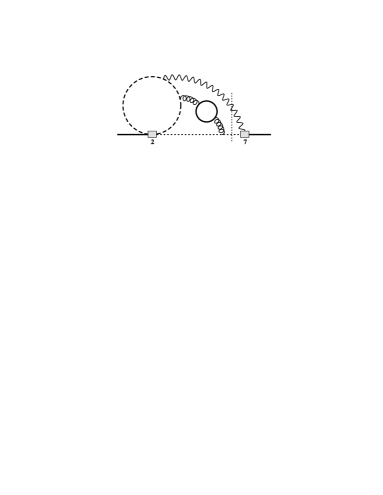
($\mathbf{a}$) [light quarks]	($\mathbf{b}$) [bottom]	($\mathbf{c}$) [charm]

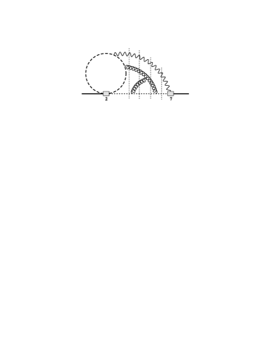
Figure 1: Sample type-I (first row) and type-II (second row) Feynman diagrams contributing to $\hat{G}^{(2)}_{27}$. Possible unitarity cuts are indicated by the vertical dotted lines. The black solid, dashed and internal dotted lines denote the $b$-quark, $c$-quark and $s$-quark propagators, respectively. In the first diagram, all the light quarks ($u$, $d$ and $s$) circulate in the closed loop on the gluon line.

We express $\hat{G}^{(2)}_{27}(z,E_{0})$ as

$$\hat{G}^{(2)}_{27}(z,E_{0})=\hat{G}^{(2),\text{type-I}}_{27}(z,E_{0})+\hat{G}^{(2),\text{type-II}}_{27}(z,E_{0}),$$ (4)

where type-I parts of $\hat{G}^{(2)}_{27}$ arise from diagrams with closed fermionic loops on the gluon lines, while the remaining contributions are called type-II (see Fig. 1). Analytical and/or numerical results for $\hat{G}^{(2),\text{type-I}}_{27}(z,E_{0})$ are available from the calculations in Refs. [16, 17, 18, 19], except for a few diagrams with four-body cuts presented in Fig. 3b of Ref. [5]. As far as type-II contributions are concerned, the calculations have been so far finalized in two limiting cases only. In Refs. [20, 21], $\hat{G}^{(2),\text{type-II}}_{27}(z,E_{0})$ was determined for large $z$, at the leading order in $1/z$. In Ref. [5], $\hat{G}^{(2),\text{type-II}}_{27}(0,0)$ was calculated. Next, an interpolation between these two limiting cases was performed to arrive at an estimate for the considered correction at the physical value of $m_{c}$, and with $E_{0}=1.6\,$GeV. The effect of the interpolated $\mathcal{O}(\alpha_{\mathrm{s}}^{2})$ contribution on the branching ratio is shown in Fig. 4 of Ref. [5]. As already mentioned, the associated uncertainty has been estimated at the $\pm 3\%$ level, which gives a significant contribution to the overall uncertainty of the SM prediction. Therefore, evaluation of the considered correction for the physical value of $m_{c}$ is important and necessary. Here, we present our results for $\hat{G}^{(2),\text{type-I}}_{27}(z,0)$, and report the status of the ongoing calculation of $\hat{G}^{(2),\text{type-II}}_{27}(z,0)$.

Once $\hat{G}^{(2),\text{type-II}}_{27}(z,0)$ is found, the next step will be to evaluate the difference between $\hat{G}^{(2)}_{27}(z,0)$ and $\hat{G}^{(2)}_{27}(z,E_{0})$ that comes from diagrams with three- and four-body cuts only. However, for $E_{0}=1.6\,$GeV, this difference is likely much smaller than $\hat{G}^{(2)}_{27}(z,0)$ itself, given that the considered interference is peaked at the maximal $E_{0}$. At the NLO, around $90\%$ of $\hat{G}^{(1)}_{27}(z,0)$ comes from the photons with $E_{\gamma}>1.6\,$GeV. Thus, the uncertainty stemming from the interpolation in $m_{c}$ should essentially disappear after an explicit determination of $\hat{G}^{(2),\text{type-II}}_{27}(z,0)$ alone.

2 Evaluation of the master integrals for arbitrary ${\boldsymbol{m}_{c}}$

After generating the Feynman diagrams with QGRAF [22] and/or FeynArts [23], we perform the Dirac and colour algebra with FORM [24] and self-written Mathematica codes, respectively. At that stage, $G^{(2)}_{27}(z,0)$ is expressed in terms of around $3\times 10^{5}$ four-loop two-scale scalar integrals in 437 families. Next, we use KIRA [25] to perform the Integration-By-Parts (IBP) [26, 27, 28] reduction. In an alternative approach, we use QGRAF together with q2e and exp [29, 30] to generate a FORM code for the amplitudes, and perform the IBP reduction with FIRE [31] and LiteRed [32]. For the most complicated families, several hundred GB of RAM and weeks of CPU are needed. Next, the Differential Equations (DEs) [33, 34, 35]

$$\frac{\text{\bf d}}{\text{\bf d}z}{M}_{n}(z,\epsilon)=\sum_{m}R_{nm}(z,\epsilon){M}_{m}(z,\epsilon)$$ (5)

are derived for the obtained Master Integrals (MIs) $M_{n}(z,\epsilon)$. Getting a closed system of DEs often requires including extra MIs. We numerically solve the DEs family-by-family, without cross-mapping the MIs among different families. Within such an approach, the total number of MIs is of order $10^{4}$. Such a large number of MIs is not an obstacle, as our calculation is fully automatized.

The DE coefficients $R_{nm}(z,\epsilon)$ are rational functions of $z$ and the dimensional regularization parameter $\epsilon$. We expand in $\epsilon$, and arrive at a DE system (analogous to the one in Eq. (5)) for functions of $z$ alone. Some of its coefficients usually contain poles on the real axis. For this reason, our integration of the DEs proceeds along ellipses in the complex $z$-plane, starting from initial conditions at large $z$, similarly to the calculations in Refs. [18, 36, 37]

Figure 2: Sample propagator-type integrals. The black solid and internal dotted lines denote the $b$-quark, and massless propagators, respectively. Unitarity cuts are shown by the thin dotted lines.

The initial conditions at large $z$ are evaluated using asymptotic expansions for $m_{c}\gg m_{b}$. It leads to tadpole integrals up to three loops with a mass scale $m_{c}$, as well as one-, two- and three-loop two-point integrals with external momentum $q^{2}=m_{b}^{2}$, and internal lines that are either massless or carry the mass $m_{b}$. In the following, we denote such two-point integrals as propagator-type integrals. For the type-I contribution, we have to compute two- and four-body cuts of the propagator-type integrals. In the type-II case, also three-body cuts are present. Sample integrals are shown in Fig. 2. The initial conditions are evaluated in an automatic manner, using the code exp [29, 30].

3 Results and progress

One can write $\hat{G}^{(2),\text{type-I}}_{27}(z,0)$ in Eq. (4) as a sum of the following three contributions

$$\hat{G}^{(2),\text{type-I}}_{27}(z,0)=3\hat{G}^{(2),\text{type-I}(\bf a)}_{27}(z,0)+\hat{G}^{(2),\text{type-I}(\bf b)}_{27}(z,0)+\hat{G}^{(2),\text{type-I}(\bf c)}_{27}(z,0),$$ (6)

as depicted in the first row of Fig. 1, for loops of the massless quarks ($u,d,s$), the bottom quark and the charm quark on the gluon propagator. After calculating the bare four-loop diagrams contributing to these quantities, we renormalize them using the known counterterms [36, 37]. One of the NLO contributions appearing in the counterterms is $\hat{G}^{(1)}_{47}$ stemming from the operator $Q_{4}=(\bar{s}_{L}\gamma_{\mu}T^{a}b_{L})\sum_{q}(\bar{q}\gamma^{\mu}T^{a}q)$. Analytical expressions for this quantity presented in Eqs. (2.4) and (B.1)-(B.2) of Ref. [5] do not include charm-quark loops. For the purpose of evaluating $\hat{G}^{(2),\text{type-I}(\bf c)}_{27}(z,0)$, we have derived an analytical expression for the charm-loop contribution to $\hat{G}^{(1)}_{47}$ up to the order ${\mathcal{O}}(\epsilon)$. An explicit formula is presented in the appendix of Ref. [1].

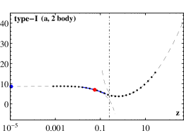
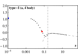
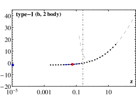
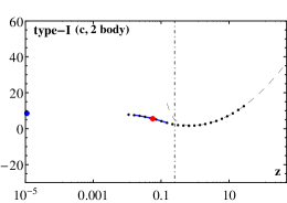
Figure 3: Plots of the functions defined in Eq. (6). See the text for explanation.

Our ${\overline{\rm MS}}$-renormalized results for all the contributions to $\hat{G}^{(2),\text{type-I}}_{27}(z,0)$ in Eq. (6) are displayed in Fig. 3, for the renormalization scale $\mu=m_{b}$. The four-body part of $\hat{G}^{(2),\text{type-I}(\bf a)}_{27}(z,0)$ is understood to contain also the three-body cut effects that enter via renormalization. As far as $\hat{G}^{(2),\text{type-I}(\bf b,c)}_{27}(z,0)$ is concerned, only the two-body parts are plotted – the remaining parts, which are induced by counterterm contributions, come in the term proportional to $\phi^{(1)}_{27}(z,\delta)$ in Eq. (3.8) of Ref. [5].

In each plot of Fig. 3, the black dots describe our numerical solutions to the DEs. The dot corresponding to the physical value of $z$ in the vicinity of $z=0.06$ is made larger and highlighted in red. For each function, its limit at $z\to 0$ is indicated by a blue dot at the vertical axis on the left. These limits read [5]:  $\left\{{\bf a\text{ [2 body]}},\,{\bf a\text{[4 body]}},\,{\bf b\text{[2 body]}},\,{\bf c\text{[2 body]}}\right\}~{}\stackrel{{\scriptstyle\scriptscriptstyle z\to 0\;\;}}{{\longrightarrow}}~{}\left\{{N}_{1},\,{N}_{2},\,{N}_{3},\,{N}_{1}\right\}$,  where ${N}_{1}=2(33727-558\pi^{2})/6561$,  ${N}_{2}\simeq 1.0640837328$,  and ${N}_{3}\simeq-1.8324081161$. The vertical dash-dotted lines indicate the $c\bar{c}$ production threshold at $z=\frac{1}{4}$. The dashed lines for $z>\frac{1}{4}$ are our large-$z$ expansions evaluated up to ${\mathcal{O}}(1/z^{2})$ [1]. Such expansions with the MIs evaluated up to $\mathcal{O}(1/z^{5})$ have served as the initial conditions at $z=20$ in our numerical solutions to the DEs. The dashed curve for $z<\frac{1}{4}$ in the upper-left plot is the known small-$z$ expansion from Ref. [17]. The blue curves in all the two-body plots are from the fit expressions published in Ref. [18].

One can see that all our two-body results are in perfect agreement with the previously published ones [17, 18]. In the four-body case, our result is new, i.e. for the first time all the contributing diagrams have been calculated for $z\neq 0$. The numerical solution in this case gets very close to the $z=0$ limit when $z$ becomes as small as $0.001$. For even lower $z$, numerical inaccuracies blow up, which we can verify by testing cancellation of the coefficients at powers of $1/\epsilon$ in the renormalization procedure. In Fig. 3, such a cancellation with a relative error of better than $\mathcal{O}(10^{-3})$ has been required for all the plotted black dots. Our large-$z$ expansions and a numerical fit for the new contribution are presented in Ref. [1].

The convergence of our large-$z$ and small-$z$ expansions (dashed lines) becomes poor in the vicinity of the threshold at $z=\frac{1}{4}$. It is most visible in the plot of $\hat{G}^{(2),\text{type-I}(\bf b)}_{27}(z,0)$. The same is true for the counterterm contributions alone, in which case using the numerical results from Refs. [36, 37] (rather than the expansions) allows us to successfully renormalize at points that are very close to the threshold.

In the type-I case, we have a simple relation $\hat{G}^{(2),\text{type-I}}_{17}(z)=-\frac{1}{6}\hat{G}^{(2),\text{type-I}}_{27}(z)$, which makes our plots in Fig. 3 directly applicable to the $Q_{1}$-$Q_{7}$ interference, too.

As far as $\hat{G}^{(2),\text{type-II}}_{27}(z)$ is concerned, its evaluation is in progress, following exactly the same lines as in the type-I case. The IBP reduction and construction of the DEs have been completed. The boundary conditions for $m_{c}\gg m_{b}$ are at the level of evaluation of three-loop propagator-type integrals with two-, three- and four-particle cuts [38].

4 Summary

We evaluated all the NNLO QCD corrections to $\mathcal{B}(\bar{B}\rightarrow X_{s}\gamma)$ stemming from diagrams with closed quark loops on the gluon lines, including cases where the unitarity cut goes through such a loop. The calculation was performed using the IBP method followed by numerically solving the DEs for the MIs. Our results for the two-body final state contributions are in agreement with the previous literature. In the four-body case, our result includes contributions that have so far been only estimated (using interpolation) at the physical value of $m_{c}$.

A calculation of the remaining (type-II) contributions for the physical $m_{c}$ is likely achievable using the same techniques as described in this work. It is being carried out by a larger team [38], currently focusing on evaluating three-loop propagator-type integrals that parameterize the boundary conditions for the DEs.

References

- [1] M. Misiak, A. Rehman and M. Steinhauser, arXiv:2002.01548.
- [2] A. Gunawardana and G. Paz, JHEP 1911 (2019) 141 [arXiv:1908.02812].
- [3] S. Watanuki et al. [Belle Collaboration], Phys. Rev. D 99 (2019) 032012 [arXiv:1807.04236].
- [4] M. Misiak, H. Asatrian, R. Boughezal, M. Czakon, T. Ewerth, A. Ferroglia, P. Fiedler, P. Gambino, C. Greub, U. Haisch, T. Huber, M. Kamiński, G. Ossola, M. Poradziński, A. Rehman, T. Schutzmeier, M. Steinhauser and J. Virto, Phys. Rev. Lett. 114 (2015) 221801 [arXiv:1503.01789].
- [5] M. Czakon, P. Fiedler, T. Huber, M. Misiak, T. Schutzmeier and M. Steinhauser, JHEP 1504 (2015) 168 [arXiv:1503.01791].
- [6] Y. S. Amhis et al. [HFLAV Collaboration], arXiv:1909.12524.
- [7] S. Chen et al. [CLEO Collaboration], Phys. Rev. Lett. 87 (2001) 251807 [hep-ex/0108032].
- [8] B. Aubert et al. [BaBar Collaboration], Phys. Rev. D 77 (2008) 051103 [arXiv:0711.4889].
- [9] J. P. Lees et al. [BaBar Collaboration], Phys. Rev. D 86 (2012) 052012 [arXiv:1207.2520].
- [10] J. P. Lees et al. [BaBar Collaboration], Phys. Rev. Lett. 109 (2012) 191801 [arXiv:1207.2690].
- [11] T. Saito et al. [Belle Collaboration], Phys. Rev. D 91 (2015) 052004 [arXiv:1411.7198].
- [12] A. Abdesselam et al. [Belle Collaboration], arXiv:1608.02344.
- [13] M. Misiak and M. Steinhauser, Eur. Phys. J. C 77 (2017) 201 [arXiv:1702.04571].
- [14] E. Kou et al. (Belle-II Collaboration), PTEP 2019 (2019) 123C01 [arXiv:1808.10567].
- [15] A. Ishikawa, talk at the “7th Workshop on Rare Semileptonic Decays”, September 4-6th, 2019, Lyon, France, https://indico.in2p3.fr/event/18646 .
- [16] Z. Ligeti, M. E. Luke, A. V. Manohar and M. B. Wise, Phys. Rev. D 60 (1999) 034019 [hep-ph/9903305].
- [17] K. Bieri, C. Greub and M. Steinhauser, Phys. Rev. D 67 (2003) 114019 [hep-ph/0302051].
- [18] R. Boughezal, M. Czakon and T. Schutzmeier, JHEP 0709 (2007) 072 [arXiv:0707.3090].
- [19] M. Misiak and M. Poradzinski, Phys. Rev. D 83 (2011) 014024 [arXiv:1009.5685].
- [20] M. Misiak and M. Steinhauser, Nucl. Phys. B 764 (2007) 62 [hep-ph/0609241].
- [21] M. Misiak and M. Steinhauser, Nucl. Phys. B 840 (2010) 271 [arXiv:1005.1173].
- [22] P. Nogueira, J. Comput. Phys. 105 (1993) 279.
- [23] J. Kublbeck, M. Bohm and A. Denner, Comput. Phys. Commun. 60 (1990) 165.
- [24] B. Ruijl, T. Ueda and J. Vermaseren, arXiv:1707.06453.
- [25] P. Maierhoefer and J. Usovitsch, arXiv:1812.01491.
- [26] F. V. Tkachov, Phys. Lett. B 100 (1981) 65.
- [27] K. G. Chetyrkin and F. V. Tkachov, Nucl. Phys. B 192 (1981) 159.
- [28] S. Laporta, Int. J. Mod. Phys. A 15 (2000) 5087 [hep-ph/0102033].
- [29] R. Harlander, T. Seidensticker and M. Steinhauser, Phys. Lett. B 426 (1998) 125 [hep-ph/9712228].
- [30] T. Seidensticker, hep-ph/9905298.
- [31] A. V. Smirnov and F. S. Chuharev, arXiv:1901.07808.
- [32] R. N. Lee, J. Phys. Conf. Ser. 523 (2014) 012059 [arXiv:1310.1145].
- [33] A. V. Kotikov, Phys. Lett. B 254 (1991) 158.
- [34] E. Remiddi, Nuovo Cim. A 110 (1997) 1435 [hep-th/9711188].
- [35] T. Gehrmann and E. Remiddi, Nucl. Phys. B 580 (2000) 485 [hep-ph/9912329].
-
[36]
M. Misiak, A. Rehman and M. Steinhauser,
Phys. Lett. B 770 (2017) 431
[arXiv:1702.07674];
A. Rehman, M. Misiak and M. Steinhauser, PoS RADCOR 2015 (2016) 049;
A. Rehman, Acta Phys. Polon. B 46 (2015) 2111. - [37] A. Rehman, Ph.D. thesis, University of Warsaw, 2015, http://depotuw.ceon.pl/handle/item/1197 .
- [38] M. Czaja, T. Huber, G. Mishima, M. Misiak, A. Rehman and M. Steinhauser, in preparation.