The Fundamental Theorem of Tropical Partial Differential Algebraic Geometry

Abstract

Tropical Differential Algebraic Geometry considers difficult or even intractable problems in Differential Equations and tries to extract information on their solutions from a restricted structure of the input. The Fundamental Theorem of Tropical Differential Algebraic Geometry states that the support of solutions of systems of ordinary differential equations with formal power series coefficients over an uncountable algebraically closed field of characteristic zero can be obtained by solving a so-called tropicalized differential system. Tropicalized differential equations work on a completely different algebraic structure which may help in theoretical and computational questions. We show that the Fundamental Theorem can be extended to the case of systems of partial differential equations by introducing vertex sets of Newton polygons.

1 Introduction

Given an algebraically closed field of characteristic zero $K$, we consider the partial differential ring $(R_{m,n},D)$, where

$$R_{m,n}=K[[t_{1},\ldots,t_{m}]]\{x_{1},\ldots,x_{n}\}$$

and $D=(\tfrac{\partial}{\partial t_{k}}\>:\>k=1,\ldots,m)$ for $n,m\geq 1$ (see Section 2 for definitions). Up to now, tropical differential algebra has been limited to the study of the relation between the set of solutions $\operatorname{Sol}(G)\subseteq K[[t]]^{n}$ of differential ideals $G$ in $R_{1,n}$ and their corresponding tropicalizations, which are certain polynomials $p$ with coefficients in a tropical semiring $\mathbb{T}[t]:=(\mathbb{Z}_{\geq 0}\cup\{\infty\},+,\min{})$ and with a set of solutions $\operatorname{Sol}(p)\subseteq\mathcal{P}(\mathbb{Z}_{\geq 0})^{n}$, see [7] and [1]. These elements $S\in\operatorname{Sol}(p)$ can be found by looking at evaluations $p(S)\in\mathbb{T}[t]$ where the usual tropical vanishing condition holds.

In this paper, we consider the case $m>1$. On this account, we work with elements in $\mathbb{Z}_{\geq 0}^{m}$, which requires new techniques. We show that considering the Newton polygons and their vertex sets is the appropriate method for formulating and proving our generalization of the Fundamental Theorem of Tropical Differential Algebraic Geometry. We remark that in the case of $m=1$ the definitions and properties presented here coincide with the corresponding ones in [1] and therefore, this work can indeed be seen as a generalization.

The problem of finding power series solutions of systems of partial differential equations has been extensively studied in the literature, but is very limited in the general case. In fact, we know from [5, Theorem 4.11] that there is already no algorithm for deciding whether a given linear partial differential equation with polynomial coefficients has a solution or not. The Fundamental Theorem, as it is stated in here, helps to find necessary conditions for the support of possible solutions.

The structure of the paper is as follows. In Section 2 we cover the necessary material from partial differential algebra. In Section 3 we introduce the semiring of supports $\mathcal{P}(\mathbb{Z}_{\geq 0}^{m})$, the semiring of vertex sets $\mathbb{T}[[t_{1},\ldots,t_{m}]]$ and the vertex homomorphism $\operatorname{Vert}\colon\mathcal{P}(\mathbb{Z}_{\geq 0}^{m})\longrightarrow\mathbb{T}[[t_{1},\ldots,t_{m}]]$. In Section 4 we introduce the support and the tropicalization maps. In Section 5 we define the set of tropical differential polynomials $\mathbb{T}_{m,n}$, the notion of tropical solutions for them, and the tropicalization morphism $\operatorname{trop}\colon R_{m,n}\to\mathbb{T}_{m,n}$. The main result is Theorem 6.1, which is proven in Section 6. The proof we give here differs essentially from that one in [1] for the case of $m=1$. In Section 7 we give some examples to illustrate our results.

In the following we will use the conventions that for a set $S$ we denote by $\mathcal{P}(S)$ its power set, and by $K$ we denote an algebraically closed field of characteristic zero.

2 Partial differential algebraic geometry

Here we recall the preliminaries for partial differential algebraic geometry. The reference book for differential algebra is [8].

A partial differential ring is a pair $(R,D)$ consisting of a commutative ring with unit $R$ and a set $D=\{\delta_{1},\ldots,\delta_{m}\}$ of $m>1$ derivations which act on $R$ and are pairwise commutative. We denote by $\Theta$ the free commutative monoid generated by $D$. If $J=(j_{1},\ldots,j_{m})$ is an element of the monoid $\mathbb{Z}^{m}_{\geq 0}=(\mathbb{Z}^{m}_{\geq 0},+,0)$, we denote $\Theta(J)=\delta_{1}^{j_{1}}\cdots\delta_{m}^{j_{m}}$ the derivative operator defined by $J$. If $\varphi$ is any element of $R$, then $\Theta(J)\varphi$ is the element of $R$ obtained by application of the derivative operator $\Theta(J)$ on $\varphi$.

Let $(R,D)$ be a partial differential ring and $x_{1},\ldots,x_{n}$ be $n$ differential indeterminates. The monoid $\Theta$ acts on the differential indeterminates, giving the infinite set of the derivatives which are denoted by $x_{i,J}$ with $1\leq i\leq n$ and $J\in\mathbb{Z}^{m}_{\geq 0}$. Given any $1\leq k\leq m$ and any derivative $x_{i,J}$, the action of $\delta_{k}$ on $x_{i,J}$ is defined by $\delta_{k}(x_{i,J})=x_{i,J+e_{k}}$ where $e_{k}$ is the $m$-dimensional vector whose $k$-th coordinate is $1$ and all other coordinates are zero. One denotes $R\{x_{1},\ldots,x_{n}\}$ the ring of the polynomials, with coefficients in $R$, the indeterminates of which are the derivatives. More formally, $R\{x_{1},\ldots,x_{n}\}$ consists of all $R$-linear combinations of differential monomials, where a differential monomial in $n$ independent variables of order less than or equal to $r$ is an expression of the form

$$E_{M}:=\prod_{\begin{subarray}{c}1\leq i\leq n\\ ||J||_{\infty}\leq r\end{subarray}}x_{i,J}^{M_{i,J}}$$ (1)

where $J=(j_{1},\ldots,j_{m})\in\mathbb{Z}_{\geq 0}^{m}$, $||J||_{\infty}:=\text{max}_{i}\{j_{i}\}=\text{max}(J)$ and $M=(M_{i,J})\in(\mathbb{Z}_{\geq 0})^{n\times(r+1)^{m}}$.

The pair $(R\{x_{1},\ldots,x_{n}\},D)$ then constitutes a differential polynomial ring. A differential polynomial $P\in R\{x_{1},\ldots,x_{n}\}$ induces an evaluation map from $R^{n}$ to $R$ given by

$$P\colon R^{n}\to R,\quad(\varphi_{1},\ldots,\varphi_{n})\mapsto P|_{x_{i,J}=\Theta(J)\varphi_{i}},$$

where $P|_{x_{i,J}=\Theta(J)\varphi_{i}}$ is the element of $R$ obtained by substituting $\Theta(J)\varphi_{i}$ for $x_{i,J}$ .

A zero or solution of $P\in R\{x_{1},\ldots,x_{n}\}$ is an $n$-tuple $\varphi=(\varphi_{1},\ldots,\varphi_{n})\in R^{n}$ such that $P(\varphi)=0$. An $n$-tuple $\varphi\in R^{n}$ is a solution of a system of differential polynomials $\Sigma\subseteq R\{x_{1},\ldots,x_{n}\}$ if it is a solution of every element of $\Sigma$. We denote by $\operatorname{Sol}(\Sigma)$ the solution set of the system $\Sigma$.

A differential ideal of $R\{x_{1},\ldots,x_{n}\}$ is an ideal of that ring which is stable under the action of $\Theta$. A differential ideal is said to be perfect if it is equal to its radical. If $\Sigma\subseteq R\{x_{1},\ldots,x_{n}\}$, one denotes by $[\Sigma]$ the differential ideal generated by $\Sigma$ and by $\{\Sigma\}$ the perfect differential ideal generated by $\Sigma$, which is defined as the intersection of all perfect differential ideals containing $\Sigma$.

For $m,n\geq 1$, we will denote by $R_{m}$ the partial differential ring

$$(K[[t_{1},\ldots,t_{m}]],D)$$

where $D=\{\tfrac{\partial}{\partial t_{1}},\ldots,\tfrac{\partial}{\partial t_{m}}\}$, and the partial differential ring $(R_{m}\{x_{1},\ldots,x_{n}\},D)$ will be denoted by $R_{m,n}$ . The proof of the following proposition can be found in  [3].

Proposition 2.1.

For any $\Sigma\subseteq R_{m,n}$, there exists a finite subset $\Phi$ of $\Sigma$ such that $\operatorname{Sol}(\Sigma)=\operatorname{Sol}(\Phi)$.

3 The semirings of supports and vertex sets

In this part we introduce and give some properties on our main idempotent semirings, namely the semiring of supports $\mathcal{P}(\mathbb{Z}_{\geq 0}^{m})$, the semiring of vertex sets $\mathbb{T}[[t_{1},\ldots,t_{m}]]$ and the map $\operatorname{Vert}\colon\mathcal{P}(\mathbb{Z}_{\geq 0}^{m})\rightarrow\mathbb{T}[[t_{1},\ldots,t_{m}]]$ which is a homomorphism of semirings.

Recall that a commutative semiring $S$ is a tuple $(S,+,\times,0,1)$ such that $(S,+,0)$ and $(S,\times,1)$ are commutative monoids and additionally, for all $a,b,c\in S$ it holds that

1. $a\times(b+c)=a\times b+a\times c$;

2. $0\times a=0$.

A semiring is called idempotent if $a+a=a$ for all $a\in S$. A map $f\colon S_{1}\longrightarrow S_{2}$ between semirings is a morphism if it induces morphisms at the level of monoids.

For $m\geq 1$, we denote by $\mathcal{P}(\mathbb{Z}^{m}_{\geq 0})$ the idempotent semiring whose elements are the subsets of $\mathbb{Z}^{m}_{\geq 0}$ equipped with the union $X\cup Y$ as sum and the Minkowski sum $X+Y=\{x+y\>:\>x\in X,y\in Y\}$ as product. We call it the semiring of supports. For $n\in\mathbb{Z}_{\geq 1}$ and $X\in\mathcal{P}(\mathbb{Z}_{\geq 0}^{m})$, the notation $nX$ will indicate $\underbrace{X+\cdots+X}_{n\ \text{times}}$. By convention we set $0X=\{(0,\ldots,0)\}$.

We define the Newton polygon $\mathcal{N}(X)\subseteq\mathbb{R}^{m}_{\geq 0}$ of $X\in\mathcal{P}(\mathbb{Z}^{m}_{\geq 0})$ as the convex hull of $X+\mathbb{Z}^{m}_{\geq 0}$. We call $x\in X$ a vertex if $x\notin\mathcal{N}(X\setminus\{x\})$, and we denote by $\operatorname{Vert}X$ the set of vertices of $X$.

Lemma 3.1.

Let $S,T\in\mathcal{P}(\mathbb{Z}_{\geq 0}^{m})$ such that $\mathcal{N}(S)=\mathcal{N}(T)$. Then $\operatorname{Vert}S=\operatorname{Vert}T$.

Proof.

Let $s\in\operatorname{Vert}S$ and we assume that $s\in\mathcal{N}(T\setminus\{s\})$. Then there are $t_{i}\in T\setminus\{s\}$, $w_{i}\in\mathbb{Z}_{\geq 0}^{m}$ and positive $\lambda_{i}\in\mathbb{R}$ adding up to 1 such that

$$s=\sum_{i}\lambda_{i}(t_{i}+w_{i}).$$

Since $t_{i}\in\mathcal{N}(S)$, we can write the $t_{i}$ as

$$t_{i}=\sum_{j}\mu_{i,j}(s_{i,j}+z_{i,j}),$$

where $s_{i,j}\in S$, $z_{i,j}\in\mathbb{Z}_{\geq 0}^{m}$ and $\mu_{i,j}\in\mathbb{R}$ are positive and adding up to 1. Thus,

$$s=\sum_{i,j}\lambda_{i}\mu_{i,j}(s_{i,j}+z_{i,j}+w_{i})=\sum_{i,j}\lambda_{i}\mu_{i,j}s_{i,j}+v,$$

where $v$ is a vector with non-negative coefficients. By excluding in the sum those summands $s_{i,j}$ which are equal to $s$, we obtain

$$s=cs+\sum_{\begin{subarray}{c}i,j\\ s_{i,j}\neq s\end{subarray}}\lambda_{i}\mu_{i,j}s_{i,j}+v$$

where $c=\sum_{i,j:s_{i,j=s}}\lambda_{i}\mu_{i,j}\in[0,1]$. If $c<1$ we can solve the equation above for $s$ to get

$$s=\sum_{\begin{subarray}{c}i,j\\ s_{i,j}\neq s\end{subarray}}\frac{\lambda_{i}\mu_{i,j}}{1-c}s_{i,j}+\frac{v}{1-c}.$$

The coefficients for the $s_{i,j}$ are positive and sum to 1, so the summation in the right hand side gives an element of $\mathcal{N}(S\setminus\{s\})$. Since $\mathcal{N}(S\setminus\{s\})$ is closed under adding elements of $\mathbb{R}_{\geq 0}^{m}$, and the coefficients of $v/(1-c)$ are non-negative, we then find that $s\in\mathcal{N}(S\setminus\{s\})$ in contradicting to the assumption that $s$ is a vertex of $S$. If $c=1$, then all $s_{i,j}$ are equal to $s$ and we get $s=s+v$. Therefore, $v=0$ and $t_{i}=s$ for each $i$, and in particular $s\in T\setminus\{s\}$, which is a contradiction. So we conclude that $s\notin\mathcal{N}(T\setminus\{s\})$ and $s$ is a vertex of $T$. ∎

Lemma 3.2.

Let $X\in\mathcal{P}(\mathbb{Z}_{\geq 0}^{m})$. Then $\mathcal{N}(\operatorname{Vert}X)=\mathcal{N}(X)$.

Proof.

By Dickson’s lemma [4, chap. 2, Thm 5], there is a finite subset $S\subseteq X$ with $X\subseteq S+\mathbb{Z}_{\geq 0}^{m}$. For such $S$, it holds that $\mathcal{N}(X)=\mathcal{N}(S)$ and by Lemma 3.1, we get $\operatorname{Vert}X=\operatorname{Vert}S$. Therefore, replacing $X$ by $S$, we may assume that $X$ is finite.

We proceed by induction on $\#X$. Indeed, if $X=\emptyset$, the statement is obvious. Let $X$ be an arbitrary finite set. If every element of $X$ is a vertex of $X$, then $\mathcal{N}(X)=\mathcal{N}(\operatorname{Vert}X)$ is trivially true. Else, take $x\in X\setminus\operatorname{Vert}X$ and let $Y=X\setminus\{x\}$. Then $\mathcal{N}(X)=\mathcal{N}(Y)$ by definition, so applying Lemma 3.1 again we obtain $\operatorname{Vert}X=\operatorname{Vert}Y$. Since $\#Y<\#X$, we may apply the induction hypothesis to $Y$, and get that $\mathcal{N}(X)=\mathcal{N}(Y)=\mathcal{N}(\operatorname{Vert}Y)=\mathcal{N}(\operatorname{Vert}X)$. ∎

Corollary 3.3.

For $X,Y\in\mathcal{P}(\mathbb{Z}_{\geq 0}^{m})$ we have $\operatorname{Vert}X=\operatorname{Vert}Y$ if and only if $\mathcal{N}(X)=\mathcal{N}(Y)$.

Lemma 3.4.

For $X,Y\in\mathcal{P}(\mathbb{Z}_{\geq 0}^{m})$, we have

$$\begin{array}[]{ccl}\operatorname{Vert}(\operatorname{Vert}(X)\cup\operatorname{Vert}(Y))&=&\operatorname{Vert}(\operatorname{Vert}(X)\cup Y)\\ &=&\operatorname{Vert}(X\cup\operatorname{Vert}(Y))\\ &=&\operatorname{Vert}(X\cup Y)\end{array}$$

and

$$\begin{array}[]{ccl}\operatorname{Vert}(\operatorname{Vert}(X)+\operatorname{Vert}(Y))&=&\operatorname{Vert}(\operatorname{Vert}(X)+Y)\\ &=&\operatorname{Vert}(X+\operatorname{Vert}(Y))\\ &=&\operatorname{Vert}(X+Y).\end{array}$$

Proof.

Let $*$ be either $\cup$ or $+$. We have the following diagram of inclusions

We show that these four sets generate the same Newton polygon. For this, it is enough to show that $X*Y\subseteq\mathcal{N}(\operatorname{Vert}(X)*\operatorname{Vert}(Y))$.

For $*=\cup$, we have $X\subseteq\mathcal{N}(\operatorname{Vert}X)\subseteq\mathcal{N}(\operatorname{Vert}(X)\cup\operatorname{Vert}(Y))$ and similarly $Y\subseteq\mathcal{N}(\operatorname{Vert}(X)\cup\operatorname{Vert}(Y))$. Hence, $X\cup Y\subseteq\mathcal{N}(\operatorname{Vert}(X)\cup\operatorname{Vert}(Y))$.

Now suppose that $*=+$. Let $t\in X+Y$, and write $t=x+y$ with $x\in X$ and $y\in Y$. Using the inclusions $X\subseteq\mathcal{N}(\operatorname{Vert}X)$ and $Y\subseteq\mathcal{N}(\operatorname{Vert}Y)$, there are $x_{i}\in\operatorname{Vert}(X)$, $y_{j}\in\operatorname{Vert}(Y)$, $u_{i},v_{j}\in\mathbb{Z}_{\geq 0}^{m}$ and $\alpha_{i},\beta_{j}\in\mathbb{R}_{\geq 0}$ satisfying $\sum_{i}\alpha_{i}=1$ and $\sum_{j}\beta_{j}=1$ such that

$$t=\sum_{i}\alpha_{i}(x_{i}+u_{i})+\sum_{j}\beta_{j}(y_{j}+v_{j}).$$

Rewriting this gives

$$t=\sum_{i,j}\alpha_{i}\beta_{j}(x_{i}+y_{j}+u_{i}+v_{j}).$$

For each pair $i,j$, the expression between parentheses is an element of $\operatorname{Vert}(X)+\operatorname{Vert}(Y)+\mathbb{Z}_{\geq 0}$ and the coefficients are non-negative and sum up to 1. This shows that $t\in\mathcal{N}(\operatorname{Vert}(X)+\operatorname{Vert}(Y))$, which ends the proof of the inclusions. ∎

Example 3.5.

An element $X\in\mathcal{P}(\mathbb{Z}_{\geq 0}^{m})$ generates a monomial ideal which contains a unique minimal basis $B(X)$ (see e.g. [4]). In general, $\operatorname{Vert}(X)\subset B(X)$ and this inclusion may be strict. Consider the set $X=\{A_{1}=(1,4),A_{2}=(2,3),A_{3}=(3,3),A_{4}=(4,1)\}\subseteq\mathbb{Z}_{\geq 0}^{2}$. The Newton polygon $\mathcal{N}(X)$ can be visualized as in Figure 1 and $\mathrm{Vert}(X)=\{A_{1},A_{4}\}$ which is a strict subset of $B(X)=\{A_{1},A_{2},A_{4}\}.$

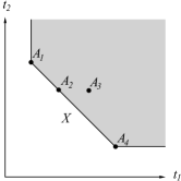
Figure 1: The Newton polygon of $X$. The vertex set of $X$ is $\{A_{1},A_{4}\}$.

We deduce from Corollary 3.3 that the map $\mathrm{Vert}\colon\mathcal{P}(\mathbb{Z}^{m}_{\geq 0})\longrightarrow\mathcal{P}(\mathbb{Z}^{m}_{\geq 0})$ is a projection operator in the sense that $\mathrm{Vert}^{2}=\mathrm{Vert}$.

Definition 3.6.

We denote by $\mathbb{T}[[t_{1},\ldots,t_{m}]]$ the image of the operator $\mathrm{Vert}$, and call its elements either vertex sets or tropical formal power series. For $S,T\in\mathbb{T}[[t_{1},\ldots,t_{m}]]$, we define

$$S\oplus T=\mathrm{Vert}(S\cup T)\quad\textrm{ and }\quad\ S\odot T=\mathrm{Vert}(S+T).$$

Corollary 3.7.

The set $(\mathbb{T}[[t_{1},\ldots,t_{m}]],\oplus,\odot)$ is a commutative idempotent semiring, with the zero element $\emptyset$ and the unit element $\{(0,\ldots,0)\}$.

Proof.

The only things to check are associativity of $\oplus$, associativity of $\odot$ and the distributive property. The associativity of $\oplus$ and $\odot$ follows from the equalities

$$S\oplus(T\oplus U)=\mathrm{Vert}(S\cup T\cup U)=(S\oplus T)\oplus U$$

and

$$S\odot(T\odot U)=\mathrm{Vert}(S+T+U)=(S\odot T)\odot U$$

which are consequences of Lemma 3.4. The distributivity follows from

$$S\odot(T\oplus U)=\operatorname{Vert}((S+T)\cup U)=\operatorname{Vert}((S+T)\cup(S+U))=(S\odot T)\oplus(S\odot U).\qed$$

Corollary 3.8.

The map $\operatorname{Vert}$ is a homomorphism of semirings. In particular, for any finite family $\{X_{i}\}_{i}$ of elements $X_{i}\in\mathcal{P}(\mathbb{Z}_{\geq 0}^{m})$, we have $\operatorname{Vert}(\sum_{i}X_{i})=\bigodot_{i\in I}\operatorname{Vert}(X_{i})$, $\operatorname{Vert}(\bigcup_{i}X_{i})=\bigoplus_{i\in I}\operatorname{Vert}(X_{i})$ and $\operatorname{Vert}(nT)=\operatorname{Vert}(T)^{\odot n}$.

Proof.

Follows directly from Lemma 3.4 and Corollary 3.7. ∎

4 The differential ring of power series and the support map

We consider the differential ring $R_{m}$ from Section 2, and the semirings $\mathcal{P}(\mathbb{Z}^{m}_{\geq 0})$, $\mathbb{T}[[t_{1},\ldots,t_{m}]]$ from Section 3. In this part we introduce the support and the tropicalization maps, which are related by the following commutative diagram

If $J=(j_{1},\ldots,j_{m})$ is an element of $\mathbb{Z}^{m}_{\geq 0}$, we will denote by $t^{J}$ the monomial $t_{1}^{j_{1}}\cdots t_{m}^{j_{m}}$. An element of $R_{m}$ is of the form $\varphi=\sum_{J\in\mathbb{Z}^{m}_{\geq 0}}a_{J}t^{J}$ with $a_{J}\in K.$

Definition 4.1.

The support of $\varphi=\sum a_{J}t^{J}\in R_{m}$ is defined as

$$\mathrm{Supp}(\varphi)=\{J\in\mathbb{Z}^{m}_{\geq 0}\ |\ a_{J}\neq 0\}.$$

For a fixed integer $n$, the map which sends $\varphi=(\varphi_{1},\ldots,\varphi_{n})\in R_{m}^{n}$ to $\mathrm{Supp}(\varphi)=(\mathrm{Supp}(\varphi_{1}),\ldots,\mathrm{Supp}(\varphi_{n}))\in\mathcal{P}(\mathbb{Z}^{m}_{\geq 0})^{n}$ will also be denoted by $\mathrm{Supp}$. The set of supports of a subset $T\subseteq R_{m}^{n}$ is its image under the map Supp:

$$\mathrm{Supp}(T)=\{\mathrm{Supp}(\varphi)\ |\ \varphi\in T\}\subseteq\mathcal{P}(\mathbb{Z}^{m}_{\geq 0})^{n}$$

Definition 4.2.

The mapping that sends each series in $R_{m}$ to the vertex set of its support is called the tropicalization map

$$\begin{array}[]{cccc}\mathrm{trop}\colon&R_{m}&\to&\mathbb{T}[[t_{1},\ldots,t_{m}]]\\ &\varphi&\mapsto&\operatorname{Vert}(\mathrm{Supp}(\varphi))\end{array}$$

Lemma 4.3.

The tropicalization map is a non-degenerate valuation in the sense of [6, Definition 2.5.1]. This is, it satisfies

1. $\operatorname{trop}(0)=\emptyset$, $\operatorname{trop}(\pm 1)=\{(0,\ldots,0)\}$,

2. $\operatorname{trop}(\varphi\cdot\psi)=\operatorname{trop}(\varphi)\odot\operatorname{trop}(\psi)$,

3. $\operatorname{trop}(\varphi+\psi)\oplus\operatorname{trop}(\varphi)\oplus\operatorname{trop}(\psi)=\operatorname{trop}(\varphi)\oplus\operatorname{trop}(\psi)$,

4. $\operatorname{trop}(\varphi)=\emptyset$ implies that $\varphi=0$.

Proof.

The first point is clear. For the second point, note that the Newton polygon has the well-known homomorphism-type property

$$\mathcal{N}(\operatorname{Supp}(\varphi\cdot\psi))=\mathcal{N}(\operatorname{Supp}(\varphi))+\mathcal{N}(\operatorname{Supp}(\psi))=\mathcal{N}(\operatorname{Supp}(\varphi)+\operatorname{Supp}(\psi)).$$

Hence, the vertices of the left hand side coincide with the vertices of the right hand side. This gives $\operatorname{trop}(\varphi\cdot\psi)=\operatorname{Vert}(\mathcal{N}(\operatorname{Supp}(\varphi)+\operatorname{Supp}(\psi)))$. That this is equal to $\operatorname{trop}(\varphi)\odot\operatorname{trop}(\psi)$ follows from Lemma 3.4. The third point follows from the observation that $\operatorname{Supp}(\varphi+\psi)\subseteq\operatorname{Supp}(\varphi)\cup\operatorname{Supp}(\psi)$ and Corollary 3.8. The last point follows from the fact that the empty set is the only set with empty Newton polygon. ∎

Definition 4.4.

For $J=(j_{1},\ldots,j_{m})\in\mathbb{Z}^{m}_{\geq 0}$, we define the tropical derivative operator $\Theta_{\operatorname{trop}}(J)\colon\mathcal{P}(\mathbb{Z}^{m}_{\geq 0})\to\mathcal{P}(\mathbb{Z}^{m}_{\geq 0})$ as

$$\Theta_{\operatorname{trop}}(J)T:=\left\{(t_{1}-j_{1},\ldots,t_{m}-j_{m})\ \left|\ \begin{array}[]{cccc}(t_{1},\ldots,t_{m})\in T,\\ t_{i}-j_{i}\geq 0\text{ for all }i\end{array}\right.\right\}$$

For example, if $T$ is the grey part in Figure 2 left and $J=(1,2)$, then informally $\Theta_{\operatorname{trop}}(J)T$ is a translation of $T$ by the vector $-J$ and then keeping only the non-negative part. It is represented by the grey part in Figure 2 right.

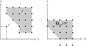
Figure 2: The operator $\Theta_{\operatorname{trop}}(J)$ for $J=(1,2)$ applied to $T$.

Since $K$ is of characteristic zero, for all $\varphi\in R_{m}$ and $J\in\mathbb{Z}^{m}_{\geq 0}$, we have

$$\mathrm{Supp}(\Theta(J)\varphi)=\Theta_{\operatorname{trop}}(J)\mathrm{Supp}(\varphi)$$ (2)

Consider a differential monomial $E_{M}$ as in (1) and $S=(S_{1},\ldots,S_{n})\in\mathcal{P}(\mathbb{Z}_{\geq 0}^{m})^{n}$. We can now define the evaluation of $E_{M}$ at $S$ as

$$E_{M}(S)=\sum_{\begin{subarray}{c}1\leq i\leq n\\ ||J||_{\infty}\leq r\end{subarray}}M_{i,J}\Theta_{\operatorname{trop}}(J)S_{i}\in\mathcal{P}(\mathbb{Z}_{\geq 0}^{m}).$$ (3)

Lemma 4.5.

Given $\varphi=(\varphi_{1},\ldots,\varphi_{n})\in R_{m}^{n}$ and a differential monomial $E_{M}$, we have $\operatorname{trop}(E_{M}(\varphi))=\operatorname{Vert}(E_{M}(\operatorname{Supp}(\varphi)))$

Proof.

By applying $\operatorname{Vert}$ to equation (2), we have

$$\operatorname{trop}(\Theta(J)\varphi_{i})=\operatorname{Vert}(\Theta_{\operatorname{trop}}(J)\mathrm{Supp}(\varphi_{i})).$$ (4)

Using the multiplicativity of trop, equation (4) and Corollary 3.8, we obtain

$$\operatorname{trop}(E_{M}(\varphi)) =\bigodot_{i,J}\operatorname{trop}(\Theta(J)\varphi_{i})^{\odot M_{i,J}}$$

$$=\bigodot_{i,J}\operatorname{Vert}(\Theta_{\operatorname{trop}}(J)\mathrm{Supp}(\varphi_{i}))^{\odot M_{i,J}}$$

$$=\operatorname{Vert}(E_{M}(\text{Supp}(\varphi))).\qed$$

Remark 4.6.

If $P=\sum_{M}\alpha_{M}E_{M}\in R_{m,n}$ and $\varphi=(\varphi_{1},\ldots,\varphi_{n})\in R_{m}^{n}$, then we can consider the upper support $US(P,\varphi)$ of $P$ at $\varphi$ as

$$US(P,\varphi)=\bigcup_{M}\left(\operatorname{Supp}(\alpha_{M})+\operatorname{Supp}(E_{M}(\varphi))\right)\in\mathcal{P}(\mathbb{Z}_{\geq 0}^{m}).$$

We now compute the vertex set of $US(P,\varphi)$ by applying the operation $\operatorname{Vert}$ and Corollary 3.8 to the above expression to find

$$\operatorname{Vert}\Bigl{(} US(P,\varphi)\Bigr{)}=\bigoplus_{M}\operatorname{trop}(\alpha_{M})\odot\operatorname{trop}(E_{M}(\varphi))$$

$$=\bigoplus_{M}\operatorname{trop}(\alpha_{M})\odot\operatorname{Vert}(E_{M}(\text{Supp}(\varphi))),$$

since $\operatorname{trop}(E_{M}(\varphi))=\operatorname{Vert}(E_{M}(\operatorname{Supp}(\varphi)))$ by Lemma 4.5. This motivates the definition of tropical differential polynomials in the next section.

5 Tropical differential polynomials

In this section we define the set of tropical differential polynomials $\mathbb{T}_{m,n}$ and the corresponding tropicalization morphism $\operatorname{trop}\colon R_{m,n}\to\mathbb{T}_{m,n}$. Let us remark that in the case of $m=1$ the definitions and properties presented here coincide with the corresponding ones in [1]. Moreover, later in Section 7 we illustrate in Example 7.2 the reason for the particular definitions given here.

Definition 5.1.

For a set $S\in\mathcal{P}(\mathbb{Z}^{m}_{\geq 0})$ and a multi-index $J\in\mathbb{Z}^{m}_{\geq 0}$ we define

$$\mathrm{Val}_{J}(S)=\operatorname{Vert}(\Theta_{\operatorname{trop}}(J)S).$$

Note that for $\varphi\in R_{m}$ and any multi-index $J$ this means that

$$\operatorname{Val}_{J}(\operatorname{Supp}(\varphi))=\operatorname{trop}(\Theta(J)\varphi).$$

In particular, $\mathrm{Val}_{J}(S)=\emptyset$ if and only if $\Theta(J)\varphi=0$. It follows from Corollary 3.8 that

$$\operatorname{Vert}(E_{M}(S))=\bigodot_{\begin{subarray}{c}1\leq i\leq n\\ ||J||_{\infty}\leq r\end{subarray}}\mathrm{Val}_{J}(S_{i})^{\odot M_{i,J}}.$$

Definition 5.2.

A tropical differential monomial in the variables $x_{1},\ldots,x_{n}$ of order less or equal to $r$ is an expression of the form

$$\epsilon_{M}=\bigodot_{\begin{subarray}{c}1\leq i\leq n\\ ||J||_{\infty}\leq r\end{subarray}}x_{i,J}^{\odot M_{i,J}}$$

where $M=(M_{i,J})\in(\mathbb{Z}_{\geq 0})^{n\times(r+1)^{m}}$.

A tropical differential monomial $\epsilon_{M}$ induces an evaluation map from $\mathcal{P}(\mathbb{Z}^{m}_{\geq 0})^{n}$ to $\mathbb{T}[[t_{1},\ldots,t_{m}]]$ by

$$\epsilon_{M}(S_{1},\ldots,S_{n})=\operatorname{Vert}(E_{M}(S))=\bigodot_{i,J}\mathrm{Val}_{J}(S_{i})^{\odot M_{i,J}}$$

where $\mathrm{Val}_{J}(S_{i})$ is given in Definition 5.1 and $E_{M}(S)$ as in (3). Let us recall that, by Corollary 3.7, we can also write

$$\epsilon_{M}(S_{1},\ldots,S_{n})=\mathrm{Vert}\biggl{(}\sum_{i,J}\mathrm{Val}_{J}(S_{i})^{\odot M_{i,J}}\biggr{)}.$$

Definition 5.3.

A tropical differential polynomial in the variables $x_{1},\ldots,x_{n}$ of order less or equal to $r$ is an expression of the form

$$p=p(x_{1},\ldots,x_{n})=\bigoplus_{M\in\Delta}a_{M}\odot\epsilon_{M}$$

where $a_{M}\in\mathbb{T}[[t_{1},\ldots,t_{m}]],a_{M}\neq\emptyset$ and $\Delta$ is a finite subset of $(\mathbb{Z}_{\geq 0})^{n\times(r+1)^{m}}$. We denote by $\mathbb{T}_{m,n}=\mathbb{T}[[t_{1},\ldots,t_{m}]]\{x_{1},\ldots,x_{n}\}$ the set of tropical differential polynomials.

A tropical differential polynomial $p$ as in Definition 5.3 induces a mapping from $\mathcal{P}(\mathbb{Z}^{m}_{\geq 0})^{n}$ to $\mathbb{T}[[t_{1},\ldots,t_{m}]]$ by

$$p(S)=\bigoplus_{M\in\Delta}a_{M}\odot\epsilon_{M}(S)=\mathrm{Vert}\Bigl{(}\bigcup_{M\in\Delta}(a_{M}+\epsilon_{M}(S))\Bigr{)}$$

The second equality follows again from Corollary 3.7. A differential polynomial $P\in R_{m,n}$ of order at most $r$ is of the form

$$P=\sum_{M\in\Delta}\alpha_{M}E_{M}$$

where $\Delta$ is a finite subset of $(\mathbb{Z}_{\geq 0})^{n\times(r+1)^{m}}$, $\alpha_{M}\in K[[t_{1},\ldots,t_{m}]]$ and $E_{M}$ is a differential monomial as in (1). Then the tropicalization of $P$ is defined as

$$\mathrm{trop}(P)=\bigoplus_{M\in\Delta}\operatorname{trop}(\alpha_{M})\odot\epsilon_{M}\in\mathbb{T}_{m,n}$$

where $\epsilon_{M}$ is the tropical differential monomial corresponding to $E_{M}$.

Definition 5.4.

Let $G\subseteq R_{m,n}$ be a differential ideal. Its tropicalization $\mathrm{trop}(G)$ is the set of tropical differential polynomials $\{\mathrm{trop}(P)\ |\ P\in G\}\subseteq\mathbb{T}_{m,n}$.

Lemma 5.5.

Given a differential monomial $E_{M}$ and $\varphi=(\varphi_{1},\ldots,\varphi_{n})\in K[[t_{1},\ldots,t_{m}]]^{n}$, we have that

$$\operatorname{trop}(E_{M}(\varphi))=\epsilon_{M}(\operatorname{Supp}(\varphi)).$$

Proof.

Follows from notations and Lemma 4.5. ∎

Consider $P=\sum_{M}\alpha_{M}E_{M}\in R_{m,n}$ and $\varphi=(\varphi_{1},\ldots,\varphi_{n})\in R_{m}^{n}$. Set $p=\operatorname{trop}(P)$ and $S=\operatorname{Supp}(\varphi)$, then $p(S)=\operatorname{Vert}(US(P,\varphi))$.

The following tropical vanishing condition is a natural generalization of the case $m=1$, but now the evaluation $p(S)$ consists of a vertex set instead of a single minimum.

Definition 5.6.

Let $p=\bigoplus_{M\in\Delta}a_{M}\odot\epsilon_{M}$ be a tropical differential polynomial. An $n$-tuple $S\in\mathcal{P}(\mathbb{Z}^{m}_{\geq 0})^{n}$ is said to be a solution of $p$ if for every $J\in p(S)$ there exists $M_{1},M_{2}\in\Delta$ with $M_{1}\neq M_{2}$ such that $J\in a_{M_{1}}\odot\epsilon_{M_{1}}(S)$ and $J\in a_{M_{2}}\odot\epsilon_{M_{2}}(S)$. Note that in the particular case of $p(S)=\emptyset$, $S$ is a solution of $p$.

For a family of differential polynomials $H\subseteq\mathbb{T}_{m,n}$, $S$ is called a solution of $H$ if and only if $S$ is a solution of every tropical polynomial in $H$. The set of solutions of $H$ will be denoted by $\mathrm{Sol}(H)$.

Proposition 5.7.

Let $G$ be a differential ideal in the ring of differential polynomials $R_{m,n}$. If $\varphi\in\operatorname{Sol}(G)$, then $\operatorname{Supp}(\varphi)\in\operatorname{Sol}(\operatorname{trop}(G))$.

Proof.

Let $\varphi$ be a solution of $G$ and $S=\operatorname{Supp}(\varphi)$. Let $P=\sum_{M\in\Delta}\alpha_{M}E_{M}\in G$ and $p=\operatorname{trop}(P)=\bigoplus_{M\in\Delta}a_{M}\odot\epsilon_{M},$ where $a_{M}=\operatorname{trop}(\alpha_{M})$. We need to show that $S$ is a solution of $p$. Let $J\in p(S)$ be arbitrary. By the definition of $\oplus$, there is an index $M_{1}$ such that

$$J\in a_{M_{1}}\odot\epsilon_{M_{1}}(S).$$

Hence, by Lemma 5.5, and multiplicative property of trop Lemma 4.3

$$J\in\operatorname{Vert}(\operatorname{Supp}(\alpha_{M_{1}}E_{M_{1}}(\varphi))).$$

Since $P(\varphi)=0$, there is another index $M_{2}\neq M_{1}$ such that

$$J\in\operatorname{Supp}(\alpha_{M_{2}}E_{M_{2}}(\varphi)),$$

because otherwise there would not be cancellation. Since $J$ is a vertex of $p(S)$, it follows that $J$ is a vertex of every subset of $\mathcal{N}(p(S))$ containing $J$ and in particular of $\mathcal{N}(\mathrm{Supp}(\alpha_{M_{2}}E_{M_{2}}(\varphi)))$. Therefore,

$$J\in a_{M_{2}}\odot\epsilon_{M_{2}}(S)$$

and because $J$ and $P$ were chosen arbitrary, $S$ is a solution of $G$. ∎

6 The Fundamental Theorem

Let $G\subset R_{m,n}$ be a differential ideal. Then Proposition 5.7 implies that $\operatorname{Supp}(\operatorname{Sol}(G))\subseteq\operatorname{Sol}(\operatorname{trop}(G))$. The main result of this paper is to show that the reverse inclusion holds as well if the base field $K$ is uncountable.

Theorem 6.1 (Fundamental Theorem).

Let $K$ be an uncountable, algebraically closed field of characteristic zero. Let $G$ be a differential ideal in the ring $R_{m,n}$. Then

$$\operatorname{Supp}(\operatorname{Sol}(G))=\operatorname{Sol}(\operatorname{trop}(G)).$$

The proof of the Fundamental Theorem will take the rest of the section and is split into several parts. First let us introduce some notations. If $J=(j_{1},\ldots,j_{m})$ is an element of $\mathbb{Z}^{m}_{\geq 0}$, we define by $J!$ the component-wise product $j_{1}!\cdots j_{m}!$. The bijection between $K^{\mathbb{Z}^{m}_{\geq 0}}$ and $R_{m}$ given by

$$\begin{array}[]{cccc}\psi\colon&K^{\mathbb{Z}^{m}_{\geq 0}}&\to&R_{m}\\ &\underline{a}=(a_{J})_{J\in\mathbb{Z}^{m}_{\geq 0}}&\mapsto&\displaystyle\sum_{J\in\mathbb{Z}^{m}_{\geq 0}}\frac{1}{J!}a_{J}t^{J}\end{array}$$

allows us to identify points of $R_{m}$ with points of $K^{\mathbb{Z}^{m}_{\geq 0}}$. Moreover, if $I\in\mathbb{Z}^{m}_{\geq 0}$, the mapping $\psi$ has the following property:

$$\Theta(I)\psi(\underline{a})=\sum_{J\in\mathbb{Z}^{m}_{\geq 0}}\frac{1}{J!}a_{I+J}t^{J}$$

which implies

$$\underline{a}=(\Theta(I)\psi(\underline{a})|_{t=0})_{I\in\mathbb{Z}^{m}_{\geq 0}}.$$

Fix for the rest of the section a finite set of differential polynomials $\Sigma=\{P_{1},\ldots,P_{s}\}\subseteq G$ such that $\Sigma$ has the same solution set as $G$ (this is possible by Proposition 2.1). For all $\ell\in\{1,\ldots,s\}$ and $I\in\mathbb{Z}_{\geq 0}^{m}$ we define

$$F_{\ell,I}=(\Theta(I)P_{\ell})|_{t_{1}=\cdots=t_{m}=0}\,\in K\big{[}x_{i,J}:1\leq i\leq n,J\in\mathbb{Z}_{\geq 0}^{m}\big{]}$$

and

$$A_{\infty}=\{(a_{i,J})\in K^{n\times(\mathbb{Z}_{\geq 0}^{m})}:F_{\ell,I}(a_{i,J})=0\textrm{ for all }1\leq\ell\leq s,I\in\mathbb{Z}_{\geq 0}^{m}\}.$$

The set $A_{\infty}$ corresponds to the formal power series solutions of the differential system $\Sigma=0$ as the following lemma shows.

Lemma 6.2.

Let $\varphi\in K[[t_{1},\ldots,t_{m}]]^{n}$ with $\varphi=(\varphi_{1},\ldots,\varphi_{n})$, where

$$\varphi_{i}=\sum_{J\in\mathbb{Z}_{\geq 0}^{m}}\frac{a_{i,J}}{J!}t^{J}.$$

Then $\varphi$ is a solution of $\Sigma=0$ if and only if $(a_{i,J})\in A_{\infty}$.

Proof.

This statement follows from formula

$$P_{\ell}(\varphi_{1},\ldots,\varphi_{n})=\sum_{I\in\mathbb{Z}_{\geq 0}^{m}}\frac{F_{\ell,I}((a_{i,J})_{i,J})}{I!}t^{I},$$

which is often called Taylor formula. See [9] for more details. ∎

For any $S=(S_{1},\ldots,S_{n})\in\mathcal{P}(\mathbb{Z}_{\geq 0}^{m})^{n}$ we define

$$A_{\infty,S}=\{(a_{i,J})\in A_{\infty}:a_{i,J}=0\textrm{ if and only if }J\notin S_{i}\}.$$

This set corresponds to power series solutions of the system $\Sigma=0$ which have support exactly $S$. In particular, $S\in\operatorname{Supp}(\operatorname{Sol}(G))$ if and only if $A_{\infty,S}\neq\emptyset$.

The sets $A_{\infty}$ and $A_{\infty,S}$ refer to infinitely many coefficients. We want to work with a finite approximation of these sets. For this purpose, we make the following definitions. For each integer $k\geq 0$, choose $N_{k}\geq 0$ minimal such that for every $\ell\in\{1,\ldots,s\}$ and $||I||_{\infty}\leq k$ it holds that

$$F_{\ell,I}\in K[x_{i,J}:1\leq i\leq n,||J||_{\infty}\leq N_{k}].$$

Note that for $k_{1}\leq k_{2}$ it follows that $N_{k_{1}}\leq N_{k_{2}}.$ Then we define

$$A_{k}=\{(a_{i,J})\in K^{n\times\{1,\ldots,N_{k}\}^{m}}:F_{\ell,I}(a_{i,J})=0$$

$$\quad\quad\textrm{ for all }1\leq\ell\leq s,||I||_{\infty}\leq k\}$$

and

$$A_{k,S}=\{(a_{i,J})\in A_{k}:a_{i,J}=0\textrm{ if and only if }J\notin S_{i}\}.$$

Proposition 6.3.

Let $S\in\mathcal{P}(\mathbb{Z}_{\geq 0}^{m})^{n}$. If $A_{\infty,S}=\emptyset$, then there exists $k\geq 0$ such that $A_{k,S}=\emptyset$.

Proof.

Assume that $A_{k,S}\neq\emptyset$ for every $k\geq 0$; we show that this implies $A_{\infty,S}\neq\emptyset$. We follow the strategy of the proof of [5, Theorem 2.10]: first we use the ultrapower construction to construct a larger field $\mathbb{K}$ over which a power series solution with support $S$ exists, and then we show that this implies the existence of a solution with the same support and with coefficients in $K$. For more information on ultrafilters and ultraproducts, the reader may consult [2].

For each integer $k\geq 0$, choose an element $(a^{(k)}_{i,J})_{1\leq i\leq n,||J||_{\infty}\leq N_{k}}\in A_{k,S}$. Fix a non-principal ultrafilter $\mathcal{U}$ on the natural numbers $\mathbb{N}$ and consider the ultrapower $\mathbb{K}$ of $K$ along $\mathcal{U}$. In other words, $\mathbb{K}=(\prod_{r\in\mathbb{N}}K)/\sim$ where $x\sim y$ for $x=(x_{r})_{r\in\mathbb{N}}$ and $y=(y_{r})_{r\in\mathbb{N}}$ if and only if the set $\{r\in\mathbb{N}:x_{r}=y_{r}\}$ is in $\mathcal{U}$. We will denote the equivalence class of a sequence $(x_{r})$ by $[(x_{r})]$. We consider $\mathbb{K}$ as a $K$-algebra via the diagonal map $K\to\mathbb{K}$. Now for each $i$ and $J$, we may define $a_{i,J}\in\mathbb{K}$ as

$$a_{i,J}=[(a_{i,J}^{(k)}:k\in\mathbb{N})]$$

where we set $a_{i,J}^{(k)}=0$ for the finitely many values of $k$ with $||J||_{\infty}>N_{k}$. For all $\ell$ and $I$, we have that $F_{\ell,I}((a^{(k)}_{i,J})_{i,J})=0$ for $k$ large enough, and so $F_{\ell,I}((a_{i,J})_{i,J})=0$ in $\mathbb{K}$, because the set of $k$ such that $F_{\ell,I}((a^{(k)}_{i,J})_{i,J})\neq 0$ is finite. Moreover, for $J\in S_{i}$ we have, by hypothesis, $a_{i,J}^{(k)}\neq 0$ for all sufficiently large $k$, so $a_{i,J}\neq 0$ in $\mathbb{K}$. On the other hand, for $J\notin S_{i}$ we have $a_{i,J}^{(k)}=0$ for all $k$, so also $a_{i,J}=0$. Now consider the ring

$$R=K\left[\begin{array}[]{l}x_{i,J}:1\leq i\leq n,J\in\mathbb{Z}^{m}_{\geq 0}\\ x_{i,J}^{-1}:1\leq i\leq n,J\in S_{i}\end{array}\right]/\left(\begin{array}[]{l}F_{\ell,I}:1\leq\ell\leq s,I\in\mathbb{Z}_{\geq 0}^{m}\\ x_{i,J}:1\leq i\leq n,J\notin S_{i}\end{array}\right)$$

The paragraph above shows that the map $R\to\mathbb{K}$ defined by sending $x_{i,J}$ to $a_{i,J}$ is a well-defined ring map. In particular, $R$ is not the zero ring. Let $\mathfrak{m}$ be a maximal ideal of $R$. We claim that the composition $K\to R\to R/\mathfrak{m}$ is an isomorphism. Indeed, $R/\mathfrak{m}$ is a field, and as a $K$-algebra it is countably generated, since $R$ is. Therefore, it is of countable dimension as $K$-vector space (it is generated as $K$-vector space by the products of some set of generators as a $K$-algebra). If $t\in R/\mathfrak{m}$ were transcendental over $K$, then by the theory of partial fraction decomposition, the elements $1/(t-\alpha)$ for $\alpha\in K$ would form an uncountable, $K$-linearly independent subset of $R/\mathfrak{m}$. This is not possible, so $R/\mathfrak{m}$ is algebraic over $K$. Since $K$ is algebraically closed, we conclude that $K=R/\mathfrak{m}$. Now let $b_{i,J}\in K$ be the image of $x_{i,J}$ in $R/\mathfrak{m}=K$. Then by construction, the set $(b_{i,J})$ satisfies the conditions $F_{\ell,I}((b_{i,J}))=0$ for all $\ell$ and $I$, and $b_{i,J}=0$ if and only if $J\notin S_{i}$. So $(b_{i,J})$ is an element of $A_{\infty,S}$, and in particular $A_{\infty,S}\neq\emptyset$. ∎

Proof of 6.1.

We now prove the remaining direction of the Fundamental Theorem by contraposition. Let $S=(S_{1},\ldots,S_{n})$ in $\mathcal{P}(\mathbb{Z}_{\geq 0}^{m})^{n}$ be such that $A_{\infty,S}=\emptyset$, i.e. there is no power series solution of $\Sigma=0$ in $K[[t_{1},\ldots,t_{m}]]^{n}$ with $S$ as the support. Then by Proposition 6.3 there exists $k\geq 0$ such that $A_{k,S}=\emptyset$. Equivalently,

$$V\left(\begin{array}[]{l}F_{\ell,I}:1\leq\ell\leq s,||I||_{\infty}\leq N_{k}\\ x_{i,J}:1\leq i\leq n,J\notin S_{i},||J||_{\infty}\leq k\end{array}\right)\subseteq V\Biggl{(}\prod_{\begin{subarray}{c}1\leq i\leq n\\ J\in S_{i}\\ ||J||_{\infty}\leq N_{k}\end{subarray}}x_{i,J}\Biggr{)}.$$

By Hilbert’s Nullstellensatz, there is an integer $M\geq 1$ such that

$$E:=\bigg{(}\prod_{\begin{subarray}{c}1\leq i\leq n\\ J\in S_{i}\\ ||J||_{\infty}\leq N_{k}\end{subarray}}x_{i,J}\bigg{)}^{M}\in\left\langle\begin{array}[]{l}F_{\ell,I}:1\leq\ell\leq s,||I||_{\infty}\leq N_{k}\\ x_{i,J}:1\leq i\leq n,J\notin S_{i},||J||_{\infty}\leq k\end{array}\right\rangle.$$

Therefore, there exist $G_{\ell,I}$ and $H_{i,J}$ in $K[x_{i,J}:1\leq i\leq n,||J||_{\infty}\leq N_{k}]$ such that

$$E=\sum_{\begin{subarray}{c}1\leq\ell\leq s\\ ||I||_{\infty}\leq k\end{subarray}}G_{\ell,I}F_{\ell,I}+\sum_{\begin{subarray}{c}1\leq i\leq n\\ J\notin S_{i}\\ ||J||_{\infty}\leq N_{k}\end{subarray}}H_{i,J}x_{i,J}.$$

Define the differential polynomial $P$ by

$$P=\sum_{\begin{subarray}{c}1\leq\ell\leq s\\ ||I||_{\infty}\leq k\end{subarray}}G_{\ell,I}\Theta(I)(P_{\ell}).$$

Then $P$ is an element of the differential ideal generated by $P_{1},\ldots,P_{s}$, so in particular $P\in G$. Since $F_{\ell,I}=\Theta(I)(P_{\ell})|_{t=0}$, there exist $h_{i}\in R_{m,n}$ such that

$$P=E-\sum_{\begin{subarray}{c}1\leq i\leq n\\ J\notin S_{i}\\ ||J||_{\infty}\leq N_{k}\end{subarray}}H_{i,J}x_{i,J}\,+\,t_{1}h_{1}+\ldots+t_{m}h_{m}.$$

Notice that $E$ occurs as a monomial in $P$, since it cannot cancel with other terms in the sum above. By construction we have $\operatorname{trop}(E)(S)=\{(0,\ldots,0)\}$. However, we have $(0,\ldots,0)\notin\operatorname{trop}(H_{i,J}x_{i,J})(S)$ because $J\notin S_{i}$, and we have $(0,\ldots,0)\notin\operatorname{trop}(t_{i}h_{i})(S)$ because the factor $t_{i}$ forces the $i$th coefficient of each element of $\operatorname{trop}(t_{i}h_{i})(S)$ to be at least $1$. Hence, the vertex $\{(0,\ldots,0)\}$ in $\operatorname{trop}(P)(S)$ is attained exactly once, in the monomial $E$, and therefore, $S$ is not a solution of $\operatorname{trop}(P)$. Since $P\in G$, it follows that $S\notin\operatorname{Sol}(\operatorname{trop}(G))$, which proves the statement. ∎

7 Examples and remarks on the Fundamental Theorem

In this section we give some examples to illustrate the results obtained in the previous sections. Moreover, we show that some straight-forward generalizations of the Fundamental Theorem from [1] and our version, Theorem 6.1, do not hold. Also we give more directions for further developments.

Example 7.1.

Let us consider the system of differential polynomials

$$\Sigma=\{ P_{1}=x_{1,(1,0)}^{2}-4\,x_{1,(0,0)}\,,\ P_{2}=x_{1,(1,1)}\,x_{2,(0,1)}-x_{1,(0,0)}+1\,,$$

$$P_{3}=x_{2,(2,0)}-x_{1,(1,0)}\}\,$$

in $R_{2,2}$. By means of elimination methods in differential algebra such as the ones implemented in the MAPLE DifferentialAlgebra package, it can be proven that

$$\operatorname{Sol}(\Sigma)=\{ \varphi_{1}(t_{1},t_{2})=2\,c_{0}\,t_{1}+c_{0}^{2}+\sqrt{2}\,c_{0}\,t_{2}+t_{1}^{2}+\sqrt{2}\,t_{1}\,t_{2}+\frac{1}{2}\,t_{2}^{2},$$

$$\varphi_{2}(t_{1},t_{2})=c_{2}\,t_{1}+c_{1}+\frac{1}{2}\,\sqrt{2}\,(c_{0}^{2}-1)\,t_{2}+c_{0}\,t_{1}^{2}$$

$$\quad+\sqrt{2}\,c_{0}\,t_{1}\,t_{2}+\frac{1}{2}\,c_{0}\,t_{2}^{2}$$

$$\quad+\frac{1}{3}\,t_{1}^{3}+\frac{1}{2}\,\sqrt{2}\,t_{1}^{2}\,t_{2}+\frac{1}{2}\,t_{1}\,t_{2}^{2}+\frac{1}{12}\,\sqrt{2}\,t_{2}^{3}\},$$

where $c_{0},c_{1},c_{2}\in K$ are arbitrary constants. By setting $c_{0}=c_{2}=0,c_{1}\neq 0$, we obtain for example that

$$(\{(2,0),(1,1),(0,2)\},\{(0,0),(0,1),(3,0),(2,1),(1,1),(0,3)\})$$

is in $\operatorname{Supp}(\operatorname{Sol}(\Sigma))$.

Now we illustrate that by our results necessary conditions and relations on the support can be found. Let $(S_{1},S_{2})\in\mathcal{P}(\mathbb{Z}_{\geq 0}^{2})^{2}$ be a solution of $\operatorname{trop}([\Sigma])$. Let us first consider

$$\operatorname{trop}(P_{1})(S_{1},S_{2})=\operatorname{Vert}(2\cdot\Theta_{\operatorname{trop}}(1,0)S_{1}\,\cup\,S_{1}).$$

If we assume that $(0,0)\in S_{1}$, then $(0,0)$ is a vertex of $S_{1}$. By the definition of a solution of a tropical differential polynomial, $(0,0)$ must be a vertex of the term $2\cdot\Theta_{\operatorname{trop}}(1,0)S_{1}$ as well, so we then know that $(1,0)\in S_{1}$. Conversely, if $(1,0)\in S_{1}$, then $(0,0)\in S_{1}$ follows. This is what we expect since the corresponding monomials in $\varphi_{1}$ vanish if and only if $c_{0}=0$.
Now consider

$$\operatorname{trop}(\Theta(1,0)P_{1})(S_{1},S_{2})=$$

$$\operatorname{Vert}(\Theta_{\operatorname{trop}}(1,0)S_{1}+\Theta_{\operatorname{trop}}(2,0)S_{1}\,\cup\,\Theta_{\operatorname{trop}}(1,0)S_{1}).$$

If we assume that $(0,0)$ is not a vertex of this expression, which implies that $(1,0)\notin S_{1}$, and $(k,0)$ is a vertex for some $k\geq 1$, then we obtain from the two tropical differential monomials that necessarily $(k,0)=(2k-1,0)$. This is fulfilled only for $k=1$ and hence, $(2,0)\in S_{1}$.

A natural way for defining $\odot$ and $\oplus$ in Section 3 would be to simply take the Newton polygon and not take its vertex set, as we do. If we do this, then some intermediate results and in particular Proposition 5.7, do not hold anymore as the following example shows.

Example 7.2.

Let $\{e_{1},\ldots,e_{4}\}$ be the standard basis for $\mathbb{Z}^{4}_{\geq 0}$. We consider the differential ideal in $R_{4,1}=K[[t_{1},\ldots,t_{4}]]\{x\}$ generated by

$$P=x_{e_{3}}x_{e_{4}}+(-t_{1}^{2}+t_{2}^{2})x_{e_{1}+e_{3}}=\frac{\partial x}{\partial t_{3}}\cdot\frac{\partial x}{\partial t_{4}}+(-t_{1}^{2}+t_{2}^{2})\frac{\partial^{2}x}{\partial t_{1}\partial t_{3}}$$

and the solution $\varphi=(t_{1}+t_{2})t_{3}+(t_{1}-t_{2})t_{4}$. Then

$$\operatorname{Supp}(\varphi)=\{e_{1}+e_{3},e_{2}+e_{3},e_{1}+e_{4},e_{2}+e_{4}\}.$$

On the other hand, for $S\in\mathcal{P}(\mathbb{Z}^{4}_{\geq 0})$ we obtain

$$\operatorname{trop}(P)(S)=\operatorname{Vert}( \operatorname{Vert}(\Theta_{\operatorname{trop}}(e_{3})S+\Theta_{\operatorname{trop}}(e_{4})S)$$

$$\cup\mathrm{Vert}(2e_{1}+\Theta_{\operatorname{trop}}(e_{1}+e_{3})S)$$

$$\cup\mathrm{Vert}(2e_{2}+\Theta_{\operatorname{trop}}(e_{1}+e_{3})S).$$

If we set $S=\operatorname{Supp}(\varphi)$, we obtain

$$\operatorname{trop}(P)(S)=\operatorname{Vert}( \operatorname{Vert}(\{2e_{1},e_{1}+e_{2},2e_{2}\})\cup\{2e_{1}\}\,\cup\{2e_{2}\}).$$

Since

$$\operatorname{Vert}(\{2e_{1},e_{1}+e_{2},2e_{2}\})=\{2e_{1},2e_{2}\},$$

every $J\in\operatorname{trop}(P)(S)$, namely $2e_{1}$ and $2e_{2}$, occurs in three monomials in $\operatorname{trop}(P)(S)$ and $S$ is indeed in $\operatorname{Sol}(\operatorname{trop}(P))$. Note that in the Newton polygon the point $e_{1}+e_{2}$, which is not a vertex, comes from only one monomial in $\operatorname{trop}(P)(S)$. Therefore, it is necessary to consider the vertices instead of the whole Newton polygon such that for instance Proposition 5.7 holds.

Remark 7.3.

The Fundamental Theorem for systems of partial differential equations over a countable field such as $\overline{\mathbb{Q}}$ does in general not hold anymore by the following reasoning. According to [5, Corollary 4.7], there is a system of partial differential equations $G$ over $\mathbb{Q}$ having a solution in $\mathbb{C}[[t_{1},\ldots,t_{m}]]$ but no solution in $\overline{\mathbb{Q}}[[t_{1},\ldots,t_{m}]]$. Taking $K=\overline{\mathbb{Q}}$ as base field, we have $\operatorname{Sol}(\operatorname{trop}(G))\neq\emptyset$ because $\operatorname{Sol}(\operatorname{trop}(G))=\operatorname{Supp}(\operatorname{Sol}(G))$ is non-empty in $\mathbb{C}$, but $\operatorname{Supp}(\operatorname{Sol}(G))=\emptyset$.

In this paper we focus on formal power series solutions. A natural extension would be to consider formal Puiseux series instead. The following example shows that with the natural extension of our definitions to Puiseux series, the fundamental theorem does not hold, even for $m=n=1$.

Example 7.4.

Let us consider $R_{1,1}=K[t]\{x\}$ and the differential ideal generated by the differential polynomial

$$P=2tx_{(1)}-x_{(0)}=2t\cdot\frac{\partial x}{\partial t}-x.$$

There is no non-zero formal power series solution $\varphi$ of $P=0$, but $\varphi=ct^{1/2}$ is for any $c\in K$ a solution. In fact, $\{\varphi\}$ is the set of all formal Puiseux series solutions.

On the other hand, let $S\in\mathcal{P}(\mathbb{Z}_{\geq 0})$. Then every point $J$ in

$$\operatorname{trop}(P)(S) =\operatorname{Vert}(\operatorname{Vert}(\{1\}+(\Theta_{\operatorname{trop}}(1)S)\cup\operatorname{Vert}(S))$$

occurs in both monomials except if $0\in J$. Hence, for every $S\in\operatorname{Sol}(\operatorname{trop}(P))$ we know that $0\notin S$. For every $I\geq 0$ we have that

$$\Theta(I)P=2tx_{(I+1)}+(2I-1)x_{(I)}\in G$$

and

$$\operatorname{trop}(\Theta(I)P)(S) =\operatorname{Vert}(\operatorname{Vert}(\{(1)\}+(\Theta_{\operatorname{trop}}((I+1)S)\cup\operatorname{Vert}(\Theta_{\operatorname{trop}}(I)S)).$$

Similarly to above, every $J\in\operatorname{trop}(\Theta(I)P)(S)$ occurs in both monomials except if $I\in J$. Therefore, $I\notin S$ and so the only $S\in\mathcal{P}(\mathbb{Z}_{\geq 0})$ with $S\in\operatorname{Sol}(\operatorname{trop}([P]))$ is $S=\emptyset$. Hence, $\operatorname{Sol}(\operatorname{trop}([P]))=\{\emptyset\}=\operatorname{Supp}(\operatorname{Sol}([P])).$

Now we want to consider formal Puiseux series solutions instead of formal power series solutions. First, $\{\operatorname{Supp}(\varphi)\}=\{\emptyset,\{1/2\}\}$. Now let us set for $S\in\mathbb{Q}^{m}$ and $J=(j_{1},\ldots,j_{m})\in\mathbb{Z}_{\geq 0}^{m}$, the set $\Theta_{\operatorname{trop}}(J)S$ defined as

$$\left\{(s_{1}-j_{1},\ldots,s_{m}-j_{m})\ \left|\ \begin{array}[]{cccc}(s_{1},\ldots,s_{m})\in S,\\ \forall 1\leq i\leq m,\ s_{i}<0\text{ or }s_{i}-j_{i}\notin\mathbb{Z}_{<0}\end{array}\right.\right\}$$

This is the natural definition, since only in the case when the exponent of a monomial is a non-negative integer, the derivative can be equal to zero. We have that $\Theta_{\operatorname{trop}}(J)(\operatorname{Supp}(\psi))=\operatorname{Supp}(\Theta(J)\psi)$ for all Puiseux series $\psi$. For $\operatorname{Val}_{J}$ and the operations $\odot$ and $\oplus$ the definitions remain unchanged.

Let $Q\in[P]$. Then

$$Q=\sum_{k\in\mathcal{I}}Q_{k}\cdot\Theta(I_{k})P$$

for some index-set $\mathcal{I}$ and $Q_{k}\in R_{m,n}$. For every $I_{k}$ we know that $\operatorname{Supp}(\varphi)=\{(1/2)\}\in\operatorname{Sol}(\operatorname{trop}(\Theta(I_{k})P))$. Let $\alpha\in\mathbb{Q}\cap(0,1)$. Then for every $J\in\operatorname{trop}(\Theta(I_{k})P)\in\mathbb{Z}_{\geq 0}$ we have that $\Theta_{\operatorname{trop}}(J)\{(1/2)\}=\Theta_{\operatorname{trop}}(J)\{(\alpha)\}+\{(1/2-\alpha)\}$. Thus, $\{\alpha\}\in\operatorname{Sol}(\operatorname{trop}(\Theta(I_{k})P))$. Since

$$\operatorname{trop}(G_{k}\cdot\Theta(I_{k})P)=\operatorname{trop}(G_{k})\odot\operatorname{trop}(\Theta(I_{k})P),$$

the solvability remains by multiplication with $G_{k}$. Therefore, $\{\alpha\}\in\operatorname{Sol}(\operatorname{trop}(G_{k}\cdot\Theta(I_{k})P))$ and consequently, $\{\alpha\}\in\operatorname{Sol}(\operatorname{trop}([P]))$. However, $\{\alpha\}\notin\operatorname{Supp}(\operatorname{Sol}([P]))$ for $\alpha\neq 1/2$.

We remark that $P$ is an ordinary differential polynomial and by similar computations as here, the straight-forward generalization from formal power series to formal Puiseux series fails for the Fundamental Theorem in [1] as well.

We conclude this section by emphasizing that the Fundamental Theorem may help to find necessary conditions on the support of solutions of systems of partial differential equations, but in general it cannot be completely algorithmic. In fact, according to [5, Theorem 4.11], already determining the existence of a formal power series solution of a linear system with formal power series coefficients is in general undecidable.

Acknowledgements

This work was started during the Tropical Differential Algebra workshop, which took place on December 2019 at Queen Mary University of London. We thank the organizers and participants for valuable discussions and initiating this collaboration. In particular, we want to thank Fuensanta Aroca, Alex Fink, Jeffrey Giansiracusa and Dima Grigoriev for their helpful comments during this week.

Research Institute for Symbolic Computation (RISC)
Johannes Kepler University Linz, Austria.

Web: risc.jku.at/m/sebastian-falkensteiner

Centro de Investigación en Matemáticas, A.C. (CIMAT)
Jalisco S/N, Col. Valenciana CP. 36023 Guanajuato, Gto, México.
e-mail: cristhian.garay@cimat.mx

Institut de recherche mathématique de Rennes, UMR 6625 du CNRS
Université de Rennes 1, Campus de Beaulieu
35042 Rennes cedex (France)
e-mail: mercedes.haiech@univ-rennes1.fr

Bernoulli Institute, University of Groningen, The Netherlands
Web: https://www.rug.nl/staff/m.p.noordman/

School of Mathematical Sciences, Queen Mary University of London
e-mail: z.toghani@qmul.ac.uk

Univ. Lille, CNRS, Centrale Lille, Inria, UMR 9189 - CRIStAL - Centre de Recherche en Informatique Signalet Automatique de Lille, F-59000 Lille, France
Web: pro.univ-lille.fr/francois-boulier

References

- [1] Fuensanta Aroca, Cristhian Garay, and Zeinab Toghani. The Fundamental Theorem of Tropical Differential Algebraic Geometry. Pacific J. Math., 283(2):257–270, 2016. arXiv:1510.01000v3.
- [2] Joseph Becker, Jan Denef, Leonard Lipshitz, and Lou van den Dries. Ultraproducts and Approximation in Local Rings I. Inventiones mathematicae, 51:189–203, 1979.
- [3] François Boulier and Mercedes Haiech. The Ritt-Raudenbush Theorem and Tropical Differential Geometry. Available at https://hal.archives-ouvertes.fr/hal-02403365, 2019.
- [4] David Cox, John Little, and Donal O’Shea. Ideals, Varieties and Algorithms. An introduction to computational algebraic geometry and commutative algebra. Undergraduate Texts in Mathematics. Springer Verlag, New York, 3rd edition, 2007.
- [5] J. Denef and L. Lipshitz. Power series solutions of algebraic differential equations. Math. Ann., 267(2):213–238, 1984.
- [6] Jeffrey Giansiracusa and Noah Giansiracusa. Equations of tropical varieties. Duke Math. J., 165(18):3379–3433, 2016.
- [7] Dima Grigoriev. Tropical differential equations. Advances in Applied Mathematics, 82:120–128, 2017.
- [8] Ellis Robert Kolchin. Differential Algebra and Algebraic Groups. Academic Press, New York, 1973.
- [9] Abraham Seidenberg. Abstract differential algebra and the analytic case. Proc. Amer. Math. Soc., 9:159–164, 1958.