XCS Classifier System with Experience Replay

Abstract.

XCS constitutes the most deeply investigated classifier system today. It bears strong potentials and comes with inherent capabilities for mastering a variety of different learning tasks. Besides outstanding successes in various classification and regression tasks, XCS also proved very effective in certain multi-step environments from the domain of reinforcement learning. Especially in the latter domain, recent advances have been mainly driven by algorithms which model their policies based on deep neural networks – among which the Deep-Q-Network (DQN) is a prominent representative. Experience Replay (ER) constitutes one of the crucial factors for the DQN’s successes, since it facilitates stabilized training of the neural network-based Q-function approximators. Surprisingly, XCS barely takes advantage of similar mechanisms that leverage stored raw experiences encountered so far. To bridge this gap, this paper investigates the benefits of extending XCS with ER. On the one hand, we demonstrate that for single-step tasks ER bears massive potential for improvements in terms of sample efficiency. On the shady side, however, we reveal that the use of ER might further aggravate well-studied issues not yet solved for XCS when applied to sequential decision problems demanding for long-action-chains.

1. Introduction

Intriguing advances of Artificial Intelligence (AI) are observable these days. One major driver that fueled recent achievements constitutes the paradigm of Reinforcement Learning (RL) combined with Deep Neural Networks (DNN). Based on this technology, human-level and even super-human results have been achieved in tremendously complex challenges such as playing Atari games (Mnih et al., 2015), defeating the world-best player in Go (Silver et al., 2017) or mastering the real-time strategy game StarCraft II (Vinyals et al., 2019). The Deep-Q-Network (DQN) (Mnih et al., 2015) is a prominent representative of this class of RL algorithms. It approximates the Q-function by means of utilizing multi-layer perceptrons (MLP) which facilitate the learning of very large state spaces in contrast to the ‘old-fashioned’ tabular approach of Q-Learning (Watkins, 1989). Since non-linear policy approximators such as used in DQN struggle with the inherent online learning nature of RL (Tsitsiklis and Van Roy, 1997), countermeasures against divergences needed to be introduced in order to allow stable learning performance (Mnih et al., 2015). One of those techniques is Experience Replay (ER). ER alleviates the problem of so-called detrimental forgetting by means of breaking the inherent correlations of consecutive samples caused by the online environment interaction of the underlying RL agent.

The XCS Classifier System (XCS) constitutes another learning approach for solving RL problems. XCS is the most investigated Learning Classifier System (LCS) these days, both in terms of empirical evaluation as well as formal theoretical analysis (Pätzel et al., 2019). XCS and direct descendants proved very successful in a variety of learning tasks, among which classification (Bernadó-Mansilla and Garrell-Guiu, 2003; Urbanowicz et al., 2014), regression (Butz et al., 2008; Stein et al., 2018), data mining (Kharbat et al., 2008; Wilson, 2001), and control (Butz et al., 2005; Bull et al., 2004; Stein et al., 2017c) appear most prominent in the literature. However, the repeated utilization of previously encountered raw experiences in XCS, as done by DQN via ER, has only barely been subject of research (cf. Sect. 2).

With a motivation slightly different from that using ER in DQN, this paper proposes and ER-extended XCS variant for real-valued state spaces and examines the potentials as well as remaining challenges of using ER within XCS.

The main scientific contribution of this work is to provide first insights in view of our underlying research hypothesis:

Hypothesis 1.

XCS with experience replay will profit from already seen raw $(s,a,r,s^{\prime})$-experiences stored in a limited replay memory in terms of i) an increased sample efficiency, and, ii) improved overall learning capabilities.

Further contributions comprise: (1) A comparative study of XCS with and without ER and DQN on well-known RL tasks from the OpenAI gym (Brockman et al., 2016). (2) A reconsideration and empirical substantiation of an already identified issue regarding the ability of XCS to learn in long-action-chain demanding RL scenarios.

We proceed with first briefly appreciating previous endeavors of using memory mechanisms and stored experiences in the context of LCS in Section 2 and then provide necessary background information regarding ER and XCS in Section 3. Based on that, we then propose an ER-extended version of XCS in Section 4. In order to confirm our hypothesis, in Section 5 results from a number of conducted empirical validation studies on single- as well as multi-step problems are reported. Section 6 closes the paper with a short summary and a delineation of future work.

2. Related Work

Our literature review did not reveal an explicit use of ER in XCS or directly related systems that are employed in online learning settings. Overall, the use of mechanisms to introduce a short- or rather long-term memory through remembering past raw experiences, e.g., state(-action)-reward(-state) tuples which are not further used for inducing a model, has barely attracted interest in the past four decades of LCS research. However, it was indeed mentioned to be a viable solution for the overgeneralization issue as identified by Lanzi in (Lanzi, 1999). Stein et al. introduced a so-called Interpolation Component to XCS in (Stein et al., 2016b, 2017b). In their work, experiences are stored as sampling points for later interpolation calculations used to guide the action-selection regime. In a later work (Stein et al., 2018), Stein et al. proposed to reuse experienced inputs with their corresponding rewards for modeling the classifier predictions by means of RBF-interpolation in a fuction approximation context. A memory mechanism was also introduced by Cliff and Ross in (Cliff and Ross, 1994) to allow for learning in non-markovian environments. Similar aspirations have been followed by Lanzi and Wilson (Lanzi, 1998; Lanzi and Wilson, 2000) as well as Pickering and Kovacs (Pickering and Kovacs, 2015) later on. Anticipation as an indirect memory mechanism gave rise to another branch of LCS, called Anticipatory LCS (ALCS). Representatives comprise ACS (Stolzmann, 1998; Butz and Stolzmann, 1999), ACS2 (Butz and Stolzmann, 2001) and YACS (Gerard et al., 2002). The prototypical scheme of an ALCS can be found in Sutton’s Dyna architecture (Sutton, 1991). ALCS constitute instances of model-based RL approaches; the model hereby is the internal representation of the environment that is retained in the agent’s memory.

3. Background

This section briefly introduces necessary concepts from the domain of RL for the sake of self-containedness. Nevertheless, due to limited space, we need to assume a certain familiarity with temporal difference learning in general as well as DQN and XCS in particular; for a more detailed introduction, the reader is referred to (Sutton and Barto, 1998), (Mnih et al., 2015) and (Wilson, 1995; Butz and Wilson, 2002), respectively.

3.1. Experience Replay & Q-Learning

Experience Replay (ER) has been first proposed by Lin in (Lin, 1992). The main motivation was to speed up learning of RL agents by introducing a straightforward to implement memory mechanism that facilitates an effective reuse of prior experiences. ER is well-recognized as being a possible solution to certain issues present in (deep) RL:

• Inherently highly correlated data samples: ER decorrelates consecutive samples (i.e., environment observations) which are the consequence of the online interaction with the environment determined by the agent’s policy $\pi$. Due to randomized re-sampling of previous experiences from a memory, ER prevents an MLP-based Q-function approximator from known issues such as parameter oscillations or even divergence (Tsitsiklis and Van Roy, 1997; Mnih et al., 2015).

• Detrimental forgetting: In environments where long-action-chains are necessary to reach the desired goal, appropriate credit-assignment of stage-setting transitions is difficult when the underlying Q-function is approximated by neural networks. Under certain circumstances, this can lead to detrimental forgetting which disrupts the sustenance of the action-chain. Given an appropriate replacement and re-sampling strategy, ER allows to remember and favor such valuable experiences, e.g., rare transitions that lead to the sparsely available reward.

In summary, ER ensures a more decorrelated and thus smoothed training of non-linear models such as (deep) neural networks, leading to (1) a higher sample efficiency, and, (2) a more comprehensive approximation of the underlying state-action-payoff landscape.

For bringing ER to work, first a so-called replay memory (RM) has to be added to the learner. An RM can be interpreted as a short-to-mid term memory (depending on its size) that stores a certain number of experiences – in its most simplistic variant this is realized by a first-in-first-out (FIFO) queue. More formally, let $RM=\langle e_{1},...,e_{N}\rangle$ be a FIFO-buffer of capacity $N$. Each experience $e_{i}\in RM$ comprises a $(s,a,r,s^{\prime})$-quadruple. In each discrete learning step, the RL agent samples an $m$-sized mini-batch of experiences from RM to repeatedly train its model on the memorized experiences. Following its most basic form, as subject of investigation in this paper, the experiences are drawn uniformly at random, i.e., $e_{i}\sim U(RM)$ As already outlined above, an individual experience $e_{i}\in RM$ is given as a $(s,a,r,s^{\prime})$-quadruple.

In the context of temporal difference learning, it is usually assumed that the learning environment is non-deterministic, i.e., characterized by stochasticity. Thus, the succeeding state $s^{\prime}$ that a learning agent perceives after executing its selected action $a_{exec}$ is not deterministic. Accordingly, the probability of the next state can be described by a transition function $P_{s^{\prime}}(s,a)=P(s^{\prime}|s,a)$. Therefore it follows that the received reward $r$ at a time is also a random variable. Let $R(s,a)$ denote the expected reward if the agent is in a current state $s$ of the state space $S$ and decides to take an action $a$ out of the action space $A$. With all the ingredients at hand, the resulting quadruple $\langle S,A,P_{s^{\prime}}(\cdot),R(\cdot)\rangle$ finally defines an MDP for which the learning agent aims to find the optimal policy $\pi^{*}$. A policy $\pi:S\rightarrow A$ can be understood as a learning agent’s decision mechanism, or as its action-selection-regime. It maps the currently observed state $s\in S$ to an action $a_{exec}\in A$ to be executed.

Q-Learning learns its optimal policy by building a so-called state-action value function, or Q-function. In its basic variant, Q-Learning builds up a table comprising Q-value estimates for each possible state-action pair. The tabular scheme prohibits the application of Q-learning to large or continuous problem spaces as it is computationally infeasible to maintain highly scaled Q-tables. Modern approaches therefore introduce approximators for learning the underlying $Q$-function while facilitating the required generalization. The model parameters $\theta$ are trained in a rather supervised manner and the resulting model then maps each state to a corresponding Q-value estimate for each possible action. Probably the most prominent approach for modern Q-value estimation is the Deep-Q-Network (DQN) algorithm (Mnih et al., 2013) which employs a DNN as the Q-function approximator, called the Q-network. The parameters $\theta$, i.e., the weights of the Q-network, are trained based on (batch) stochastic gradient descent using a quadratic error term as loss function. However, as already discussed above, certain issues arise when non-linear function approximators, such as MLPs, are utilized to model the Q-function. For that reason, ER was introduced to the DQN algorithm, along with further modifications to ensure data efficient and stable learning (for more details cf. (Mnih et al., 2013; Mnih et al., 2015)). ER allows to re-sample minibatches from the RM which are then used to train the Q-network in sequence or batch-wise using the squared error term (or its expected value in case of batch gradient descent) between the target $r+\gamma\max_{a^{\prime}}Q(s^{\prime},a^{\prime},\theta)$ and the current Q-network’s estimate $Q(s,a,\theta)$, effectively stabilizing the training process.

3.2. XCS Classifier System in a Nutshell

The XCS classifier system (Wilson, 1995, 1998) is an evolutionary rule-based machine learning system. It belongs to the family of Michigan-style LCS which are due to Holland (Holland and Reitman, 1978; Holland, 1986). The XCS is an accuracy-based system what distinguishes it from its so-called strength-based relatives such as ZCS (Wilson, 1994). Many extensions to the original XCS have been proposed. One enhancement of special interest is the introduction of interval predicates along with slight modifications in order to deal with real-valued inputs (Wilson, 2000) – the resulting extension is called XCS for real valued inputs (XCSR). The next paragraphs very briefly introduce the general learning scheme of XCS.

At the heart of XCS a population $[P]\coloneq\{cl_{i}\}_{i\in\mathbb{N}}$ of rules is maintained. Historically, rules are also termed ‘classifiers’. Here each rule is denoted by $cl_{i}$ or simply $cl$. A classifier comprises:

• A condition $cl.C\subseteq S$ determining a subset of the state space $S$ for which this rule matches

• An action $cl.a\in A$ from the action space this rule advocates

• Quality parameters to be learned online:

  • A payoff prediction $cl.p$ which can be a simple scalar or computed by a predictive model

  • An estimate of the absolute prediction error $cl.\epsilon$

  • A rule’s fitness $cl.F$, estimating its niche-relative payoff prediction accuracy

• Further book-keeping statistics:

  • $cl.exp$ denotes the number of conducted reinforcements

  • $cl.ts$ is a time-stamp updated every time this classifier was a candidate for the GA

  • $cl.as$ estimates the average size of action sets this classifier has been part of

  • $cl.num$ counts successful subsumption operations

XCS’s working principle can be described as the result of a complex interaction between several components: Local learning of the payoff prediction models, global optimization of the classifiers’ locality (i.e., the size of their conditions $cl.C$), collective decision making based on a fitness-weighted mixing of the matching rules’ predictions, as well as population-wide replacement (i.e., insertion and deletion) mechanisms to satisfy the population size constraint $\sum_{cl\in[P]}cl.num\leq N$. The numerosity $cl.num$ is a counter of successful subsumptions which further facilitates generalization over the state space (Wilson, 1998). In standard XCS, local learning is conducted by employing a Widrow-Hoff learning scheme to the quality parameters of rules matching the current state $s$ (hold in a so-called match set $[M]\subseteq[P]$) and whose action was selected for being executed (hold in another subset called the action set $[A]\subseteq[M]$). A steady-state niche Genetic Algorithm (GA) in combination with a population-wide (panmictic) classifier replacement mechanism takes care of global optimization toward maximally general and accurate rules. The inference or action-selection step greedily selects the highest fitness-weighted prediction sum of all classifiers in $[M]$ that vote for the same action. Therefor a system prediction for each action present in $[M]$ is stored in the prediction array (PA). In order to account for the exploration/exploitation dilemma, actions are drawn by chance with a certain probability (e.g., using $\epsilon$-greedy policy) as usual for model-free RL agents.

XCS is very flexible in terms of the learning tasks it is able to solve – thereby only demanding for a few straightforward modifications. XCS is not restricted to just RL problems (single- or multi-step) but has also been very successfully applied to supervised classification and regression tasks (Bernadó-Mansilla and Garrell-Guiu, 2003; Urbanowicz et al., 2014; Butz et al., 2008; Stein et al., 2018), data mining (Wilson, 2001; Kharbat et al., 2008) as well as unsupervised clustering (Tamee et al., 2007) and even autoencoding (Preen et al., 2019).

Algorithm 1 provides a concise description of one iteration through XCS’s main learning loop. This loop is passed through as long as the selected termination criteria are not met, e.g., a maximum number of learning steps or convergence.

Algorithm 1 XCS learning iteration, adapted from (Butz and Wilson, 2002)

1:Observe environmental state $s_{t}$ at time $t$

2:Create match set $[M]\subseteq[P]$ for $s_{t}$, i.e., $[M]\coloneq\{cl_{i}|s_{t}\in cl_{i}.C\}$

3:Create $PA$ from $[M]$, i.e., $PA(a)=\frac{\sum_{cl\in[M]|cl.a=a}cl.p\cdot cl.F}{\sum_{cl\in[M]|cl.a=a}cl.F}$

4:if $U[0,1]<\epsilon$ then

5:     Select random action, i.e., $a_{exec}=rand(A)$

6:else

7:     Select best action, i.e., $a_{exec}=\text{argmax}_{a}PA(a)$

8:end if

9:Create action set $[A]\subseteq[M]$, i.e., $[A]\coloneq\{cl_{i}|cl_{i}.a=a_{exec}\}$

10:Execute $a_{exec}$ on the environment

11:Observe environmental reward $r_{t}$

12:if $[A]_{t-1}\neq\emptyset$ then

13:     $P\leftarrow r_{t-1}+\gamma\cdot\text{argmax}_{a}PA(a)$

14:     Update all $cl\in[A]_{t-1}$ using $P$

15:     if $t-\frac{\sum_{cl\in[A]_{t-1}}cl.num\cdot cl.ts}{\sum_{cl\in[A]_{t-1}}cl.num}>\theta_{GA}$ then

16:         Run GA on $[A]_{t-1}$ considering $s_{t-1}$

17:     end if

18:end if

19:if end of episode then

20:     $P\leftarrow r_{t}$

21:     Update all $cl\in[A]$ using $P$

22:     if $t-\frac{\sum_{cl\in[A]}cl.num\cdot cl.ts}{\sum_{cl\in[A]}cl.num}>\theta_{GA}$ then

23:         Run GA on $[A]$ considering $s_{t}$

24:     end if

25:     $[A]_{t-1}\leftarrow\emptyset$

26:else

27:     $[A]_{t-1}\leftarrow[A]$

28:     $r_{t-1}\leftarrow r_{t}$

29:     $s_{t-1}\leftarrow s_{t}$

30:end if

4. XCS with Experience replay

One important aspect to note is that the credit assignment step in XCS shares obvious similarities to the Q-value update (Wilson, 1995; Lanzi, 2002). The most distinguishing aspect, however, is the GA-based state-space generalization capability of XCS compared to tabular Q-learning. The rules’ conditions $cl.C$ essentially partition the state space $S$ which leads to a local learning intuition. This means that not one global approximation of the state-action-payoff map $S\times A\rightarrow P$ is learnt at once. Instead, the problem space is partitioned and individual niches are approximated by several, partially overlapping classifiers, following the divide-and-conquer principle. The actual partitioning is optimized by the employed GA. Its selection pressure strongly depends on the niche-relative accuracy of the candidate rules ($cl\in[A]$). A rule’s accuracy follows a sort of inverse relationship to its prediction error estimate $cl.\epsilon$, more precisely:

(1) $$cl.\kappa=\begin{cases}1&,~{}cl.\epsilon<\epsilon_{0}\\ \alpha\bigl{(}\frac{\epsilon}{\epsilon_{0}}\bigr{)}^{-\nu}&,~{}\text{otherwise}\end{cases}$$

From that it follows, that the appropriate generalization toward maximally general and at the same time maximally accurate rules depends strongly on the data efficiency of the employed learning mechanisms; in case of standard XCS the Widrow-Hoff, also known as least mean squares method. This in turn implies that an increased convergence rate of the classifiers’ error estimates $cl.\epsilon$ – e.g., due to ER – results in faster perceptibility of an appropriate fitness signal fueling the GA during classifier generalization.

For that reason, we propose to leverage the potentials of ER regarding its ability to increase data efficiency by repeatedly feeding the learning rules with memorized experiences. Therefor, we modified the main learning loop of XCS as given in Algorithm 2:

Algorithm 2 XCS with ER

1:Initialize $RM$ with capacity $|RM|=N$ as FIFO-queue

2:repeat

3:     Follow Alg. 1 until line 11 $\triangleright$ see Alg. 1

4:// Add experience to $RM$

5:     if $[A]_{t-1}\neq\emptyset$ then $\triangleright$ Multi-step problem

6:         $RM\coloneq RM\cup\{(s_{t-1},a_{t-1},r_{t-1},s_{t})\}$

7:         $s_{t-1}\leftarrow s_{t}$

8:         $a_{t-1}\leftarrow a_{exec}$

9:         $r_{t-1}\leftarrow r_{t}$

10:         $[A]_{t-1}\leftarrow[A]$

11:     else$\triangleright$ Single-step problem

12:         $RM\coloneq RM\cup\{(s_{t},a_{exec},r_{t})\}$

13:     end if

14:     Possibly drop oldest experience $\triangleright$ FIFO-queue

15:// Sample minibatch of size $m$ from $RM$

16:     $B_{exp}\coloneq\{e_{j}|e_{j}\in RM\land e_{j}\sim U(RM)\}_{j=1\dots m}$

17:     for $e_{j}:B_{exp}$ do

18:         Do ExperienceReplay($e_{j}$) $\triangleright$ see Alg. 3

19:     end for

20:     if end of episode then $\triangleright$ Always true for single-step

21:         $[A]_{t-1}\leftarrow\emptyset$

22:     end if

23:until termination criteria met

Algorithm 3 ER reinforcement

1:procedure ExperienceReplay($e_{j}$)

2:     Read $e_{j}\coloneq(s,a_{exec},r,s^{\prime})$ quadruple

3:     Create match set $[M]\coloneq\{cl|s\in cl.C\land cl\in[P]\}$

4:     Create action set $[A]\coloneq\{cl|cl.a=a_{exec}\land cl\in[M]\}$

5:     if $s^{\prime}$ is not terminal then

6:         Create match set $[M]^{\prime}\coloneq\{cl|s^{\prime}\in cl.C\land cl\in[P]\}$

7:         Create $PA$ with $PA(a)=\frac{\sum_{cl\in[M]^{\prime}|cl.a=a}cl.p\cdot cl.F}{\sum_{cl\in[M]^{\prime}|cl.a=a}cl.F}$

8:         $P\leftarrow r+\gamma\cdot\text{argmax}_{a}PA(a)$

9:     else if $s^{\prime}$ is terminal $|$ not existent then $\triangleright$ Single-step

10:         $P\leftarrow r$

11:     end if

12:// Update all $cl\in[A]$ using $P$

13:     for $cl:[A]$ do

14:         $cl.exp\leftarrow cl.exp+1$

15:         $cl.\epsilon\leftarrow cl.\epsilon+\beta\cdot(|P-cl.p|-cl.\epsilon)$

16:         $cl.p\leftarrow cl.p+\beta\cdot(P-cl.p)$

17:         $cl.F\leftarrow cl.F+\beta\cdot(cl.\kappa^{\prime}-cl.F)$

18:         $cl.as\leftarrow cl.as+\beta\cdot(\sum_{cl\in[A]}cl.num-cl.as)$

19:     end for

20:     if $t-\frac{\sum_{cl\in[A]}cl.num\cdot cl.ts}{\sum_{cl\in[A]}cl.num}>\theta_{GA}$ then

21:         Run GA on $[A]$ considering $s$

22:     end if

23:end procedure

As can be seen from Algorithms 2 and 3, mainly the credit assignment and the GA application frequency have been modified. Instead of the conventional one-pass learning approach which is based on the most recently seen experience $e_{t}=(s_{t-1},a_{t-1},r_{t-1},s_{t})$ or $e_{t}=(s_{t},a_{exec},r_{t})$ for multi- and single-step problems, respectively, a predefined number of previous experiences $e_{j}\in RM$ is used. The current experience is only added to the limited replay memory $RM$ which is realized as a FIFO-buffer. In its simple form, as introduced in this paper, all experiences stored in $RM$ get the same chance of being selected. This essentially ensures that the underlying dynamics in terms of the sample distribution of the learning problem is not affected, as would be the case when more sophisticated concepts such as prioritized replay (Schaul et al., 2015) would be employed (which is not subject of this initial work). The actual learning then happens on the basis of a minibatch $B_{exp}$ of predefined size $m$ which is sampled uniformly at random from the $RM$. ER reinforcement (cf. Alg. 3) is then executed for each experience $e_{j}\in B_{exp}\subseteq RM$. Depending on whether XCS is asked to solve a single- or multi-step (sequential) problem, different payoff values $P$ are considered for the credit assignment or update steps as usual. For each experience $e_{j}\in B_{exp}$ which is going to be replayed, the employed steady-state niche GA gets a chance of being invoked. This effectively increases the GA frequency by a factor $m$, i.e., the number of experiences drawn from $RM$ for the minibatch. Increased GA application exerts higher evolutionary pressure to the population $[P]$, more precisely to the niches which are hit by the drawn replay experiences.

In a fully uniformly sampled state space, ER in XCS is expected to directly increase the convergence speed. As we will show in the subsequent evaluation section, for problems subject to non-uniform problem space sampling, the above assumption might not hold. Tasks belonging to the latter category are almost always given in sequential problems (recall the above discussion of the highly correlated consecutive samples). In a multi-step scenario, the application of ER was expected to support the learning progress especially in the presence of sparse reward signals. But as we will demonstrate below, ER at the same time bears the risk of boosting the well-recognized issue of premature overgeneralization (Lanzi, 1999; Barry, 2002), which hinders XCS from sustaining long-action-chains. In the following, XCS using ER is denoted as XCS-ER. The capacity of the RM and the size of the resampled mini-batches for conducting ER was fixed to $N=50k$ $m=4$ in this work, respectively. Furthermore, we applied a warm-up phase over the first 1000 learning steps to fill the RM. Learning only starts after this warm-up.

5. Evaluation

This section summarizes the results we obtained on a variety of experiments conducted in order to assess the potentials of XCS using ER. We conducted experiments on three well-known single-step problems (see Sect. 5.1) as well as on three challenging tasks from the domain of multi-step RL (see Sect. 5.2). All conducted experiments have been repeated 30 times with different random seeds. The tables below (Tab. 1) and in the supplemental material indicate the repetition means as well as the observed standard deviations. Standard XCS without ER serves as baseline for statistical assessment. First, we conducted Shapiro-Wilk tests to check for normal distribution of the repetition means. In the positive case, paired one-sided t-tests between the baseline and XCS-ER (and additionally DQN for multi-step) have been selected to judge statistical significance of the differences. Otherwise, the Wilcoxon signed-rank test was conducted. During the multi-step experiments, a DQN baseline implementation as provided by OpenAI (Brockman et al., 2016) served as further opponent. For comparability reasons, vanilla DQN as proposed by Mnih et al. (Mnih et al., 2015) with standard ER has been chosen. The plots as depicted below show the learning curves of the compared algorithms over the entire learning period. Error bars indicate the standard deviation. For the single-step experiments, the learning progress is depicted in terms of the aggregated reward as well as the system prediction error as commonly done in the LCS literature. To evaluate the progress in the multi-step scenarios, the last 100-episode reward mean is plotted as often done in the RL field. The axis scales depend on the reward schemes of the problem under investigation.

5.1. Results on Single-step Problems

First, XCS-ER was evaluated on three benchmark problems well-known in the context of LCS-research. These are: (1) The real-multiplexer problem (RMP) (Wilson, 2000; Stone and Bull, 2003), (2) the Mario classification problem as introduced in (Stein et al., 2017a), and, (3) the Wisconsin Breast Cancer (WBC) data set from the domain of medical data mining (Kharbat et al., 2008; Wilson, 2001). The RMP is a challenging problem for machine learning systems, since it exhibits characteristics such as heterogeneity (multiple niches with equal actions) and epistasis (feature interactions) (Urbanowicz and Moore, 2015). RMP is a real-valued binary classification problem. In this paper, we used the $k=6$ RMP variant. The Mario problem is a generalization of the checkerboard problem (Stone and Bull, 2003), a well-known benchmark for assessing LCS. It comprises a 16x16 pixel-art of Mario, which entails seven possible actions (the different colors) and allows for different generalizations in different niches (e.g., the blue trousers in contrast to the yellow knobs). Mario constitutes a two-dimensional real-valued multi-class classification problem. The WBC data set from the UCI repository (Lichman, 2013) is probably one of the most famous benchmarks for classification. It consists of 10 integer-valued input dimensions indicating several features from a breast cancer diagnostics assessment and a binary label for ‘malignant’ or ‘benign’ . Usually, other types of modern LCS would be preferred for mining such data, e.g., ExSTRaCS (Urbanowicz et al., 2014; Urbanowicz and Moore, 2015) or BioHEL (Bacardit et al., 2009). However, we selected this data set, since (1) XCS was already applied on it and therefore we could make use of tuned hyperparameter-settings, and, (2) we pursue the aim to demonstrate that ER can improve XCS’s ability for stream mining of real-world data. Furthermore, the presented ER extension appears to be straightforwardly adaptable for any supervised LCS directly descending from XCS.

For each of the single-step problems, a binary reward scheme has been applied. For each correctly proposed action a reward of 1000 was payed. Otherwise, 0 was returned. The unordered bound hyperrectangular condition representation has been chosen. Further hyperparameters have been adopted from the literature and can be found in (Wilson, 2000; Stone and Bull, 2003), (Stein et al., 2017a) and (Wilson, 2001; Kharbat et al., 2008) for RMP, Mario and WBC, respectively, as well as in this paper’s supplemental material.

Table 1 provides the observed results. For the single-step tasks we assessed XCS for four standard figures of merit: (1) The average reward received at the end of the learning period. (2) The average system error between the predicted and the actually received reward. (3) The average size of the population, denoted $|[P]|$. And finally, (4) the average generality of the classifiers in $[P]$, which is equivalent to the average volume of the classifier conditions.

Table 1. Overall results for the single-step environments. Reward, system error, population size and generality is indicated. All entries show the means $\pm$1SD over the 30 repetitions. Arrows indicate whether the metric increased or decreased compared to standard XCS. * (**) indicate statistically significant differences, i.e., a p-value ¡ $\alpha$ = 0.05 (0.01). Bold entries highlight improvements over the baseline.

Mario	Reward	Sys. Err.	$|[P]|$	Generality
XCS-ER-8	959.67$\uparrow$** $\pm$1.72	49.17$\downarrow$** $\pm$1.90	2151.76$\downarrow$** $\pm$19.5	0.0078$\downarrow$** $\pm$0.0002
XCS-ER-4	944.60$\uparrow$** $\pm$2.69	69.58$\downarrow$** $\pm$2.94	2314.33$\downarrow$** $\pm$16.39	0.0085$\downarrow$** $\pm$0.0002
XCS	880.12 $\pm$3.54	188.81 $\pm$3.70	2759.87 $\pm$28.47	0.0092 $\pm$0.0002
6-RMP	Reward	Sys. Err.	$|[P]|$	Generality
XCS-ER	957.64$\uparrow$** $\pm$3.10	67.18$\downarrow$** $\pm$5.89	281.37$\downarrow$** $\pm$11.58	0.0010$\uparrow$** $\pm$4.96E-5
XCS	925.97 $\pm$12.82	147.37 $\pm$18.91	409.65 $\pm$20.56	0.0008 $\pm$5.28E-5
WBC	Reward	Sys. Err.	$|[P]|$	Generality
XCS-ER	989.34$\downarrow$** $\pm$0.72	15.83$\downarrow$** $\pm$0.77	3714.27$\downarrow$** $\pm$27.20	3.46E-7$\uparrow$** $\pm$ 1.35E-7
XCS	996.42 $\pm$0.76	24.01 $\pm$1.82	3942.97 $\pm$26.24	1.00E-7 $\pm$2.86E-8

As can be noted from Table 1, XCS-ER significantly outperforms standard XCS without ER in nearly all figures of merit for any of the three examined problems. For the Mario pixel art problem, we exemplarily doubled the size of the minibatch to $m=8$ in order to fathom whether more extensive replay bears higher potential for improvements. Although the one conducted preliminary experiment promises further improvements, this aspect needs to be investigated further. Considering the generality metric, it becomes apparent that for the Mario environment, significantly smaller average generalities have been observed (for detailed plots see supplemental material). However, if we judge this result in conjunction with the observed progress of the population size, it appears that subsumption can act more properly which results in a significantly decreased average number of rules in the population. Paired with the highly improved reward and system error metrics, we conclude that ER has supported XCS to reach a more appropriate degree of rule specification much quicker, thereby increasing sample efficiency as hypothesized at the beginning.

Although the overall performance of XCS on single-step problems can be significantly improved through ER, inspection of the learning plots (Fig. 1) reveals one interesting insight. When starting off tabula rasa, i.e., with an empty ruleset $[P]$, during the very initial learning phases XCS-ER appears to have slightly inferior performance in terms of reward and system error. This is attributed to: (1) The initial 1000 steps comprising a warm-up phase where no learning happens. (2) The higher evolutionary pressure exerted through the use of ER. The GA has $m$-times more opportunities to act, which results in more transient rules due to a poor fitness signal resulting in more random variations. This shortly blows up the population at the beginning. However, the more frequently applied GA also increases the generalization pressure, since at the same time the error estimates converge more quickly what effectively leads to a stronger fitness signal. The additional plots as given in the supplemental material corroborate this first conjecture, which yet needs more research. Especially for the WBC data set, of which already standard XCS is very capable, the abovementioned effect resulted in a slightly but indeed significant decrease of the average reward received over the entire learning period, even if the prediction error itself can be significantly improved. In order to attenuate this effect, recently proposed interpolation-based action-selection and classifier generation schemes (Stein et al., 2016a; Stein et al., 2017b), found to effectively decrease initial prediction errors, could be employed.

It can be concluded that XCS for real-valued inputs using ER substantially increases the learning efficiency in single-step problems.

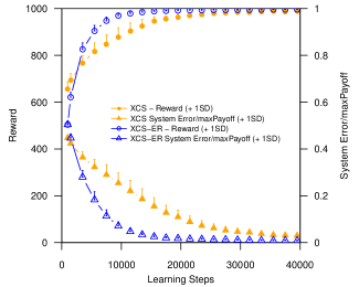
(a) $k=6$-Real Multiplexer

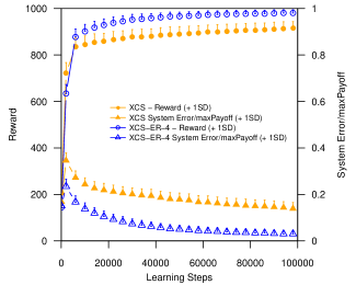
(b) Mario Pixel Art (Stein et al., 2017a)

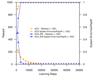
(c) WBC classification

Figure 1. XCS vs. XCS-ER on single-step problems.

5.2. Results on Multi-step Problems

XCS has been found to reliably solve certain grid-like multi-step problems. However, literature evaluating XCS on well-known RL problems such as CartPole or MountainCar remains sparse. We used the OpenAI gym (Brockman et al., 2016) to compare XCS and XCS-ER against standard DQN. Three challenging environments serve as testbeds. (1) The nChain problem of length $n=16$. (2) The pole balancing cart control problem (CartPole). (3) The MountainCar environment. Due to lack of space, we refer the reader to (Sutton and Barto, 1998; Strens, 2000) and the OpenAI gym documentation (Brockman et al., 2016) for a detailed description of the tasks. Slight modifications to the environments had to be carried out which do not considerably change the problems’ complexities. Please confer the supplemental material for details regarding the modifications and the applied hyperparameter configurations.

The plots of the observed learning curves as shown in Figure 2 summarize the results. In order to provide a comparability with DQN, we show the overall total mean (OTM) which calculates as the 100-episode mean of the received return (accumulated reward) per episode (as used in the OpenAI gym) averaged over the 30 experiment repetitions. Additionally, in the supplemental material a similar result table containing the same metrics as for the single-step case is provided. There, also the number of divergences observed across the repetitions is indicated in the last column. A divergence here is defined as an experimental run (until the max. number of steps is reached) where the algorithm was not able to find a proper solution and got stuck in local optima, i.e., never converged.

The results reveal that XCS with and without ER struggles in solving the examined multi-step environments (cf. the reported number of diverged runs). Especially in the MountainCar environment, for 29 out of 30 runs XCS was not able to solve the problem. In contrast, DQN only diverged 3 times. This observation was attributed to the well-known over-generalization issue of XCS when applied to certain multi-step scenarios. Due to the non-uniform sampling in sequential problems, classifiers quickly tend to overgeneralize across environmental niches (Lanzi, 1999; Barry, 2002). This is because a prevalent lack in negative reward signals for situations that only barely or do not occur at all, which hinders XCS from identifying rules to be inaccurate in those regions. This in turn blurs the fitness signal on which the employed GA bases its coverage or generality optimization. According to Wilson’s generalization hypothesis (Wilson, 1995), XCS will generalize rules as long as the niche-relative fitness does not decrease. Without the ability to reliably identify so-called (strong) overgenerals (Kovacs, 2000), XCS continues to create even more general offspring rules which eventually swamp the population – in the worst case leading to divergences. In presence of a sparse reward signal, as artificially produced for the MountainCar environment in this paper, this issue becomes even more dramatic. Exactly this phenomenon also constitutes a reason why XCS faces difficulties to sustain long-action-chains in multi-step environments (Barry, 2002).

Our initial hypothesis states that we suspected that the application of ER would increase XCS’s learning capability and thus attenuate this effect. Actually, quite the contrary appeared to be true. ER increases sample efficiency by repeatedly feeding already made experiences into the credit assignment procedures (in case of XCS, the Widrow-Hoff update rule). With an already skewed underlying experience or sample distribution, the minibatches drawn uniformly from the RM share the same skewness. Breaking the correlations between consecutively encountered experiences alone does not result in a more uniform prior data distribution regarding the samples from the state-action-reward landscape $S\times A\rightarrow\mathbb{R}$. In theory, XCS should not suffer from consecutive samples to the same extent as global approximators such as DQN do, since it already breaks the overall problem space up into several environmental niches for which an individual model (collectively determined by the residing classifiers) is sought each. However, in practice it turns out that XCS is not yet at this point, which clearly requests for further research in this regard. To corroborate our abovementioned rationale, we modified the initial states of the environments to be more randomly distributed among the state space $S$. Therefore, we employed the teletransportation technique (Lanzi, 1999). As can be seen from the corresponding plots showing the learning progress (see Fig. 2), effectively changing the prior state distribution through teletransportation completely eradicates the occured divergences for XCS in the nChain and MountainCar scenario. Naturally, also DQN benefits from this treatment. Considering the CartPole environment, a more uniform distribution of the initial states dramatically increases the problem complexity. Now, a controller is sought which can stabilize the pole from any position, at any velocity and any starting angle and velocity of the pole. This demands for a much longer learning period, which is not subject of the present work. However, overall XCS-ER appears to still benefit from ER considering the OTM metric compared to standard XCS.

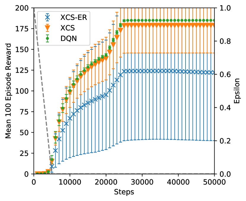
(a) XCS vs. XCS-ER in 16Chain.

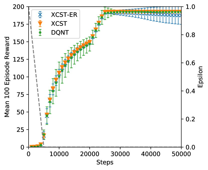
(b) XCST vs. XCST-ER in 16Chain.

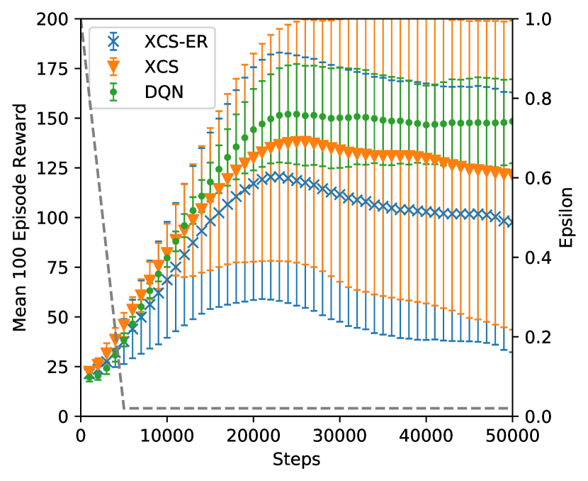
(c) XCS vs. XCS-ER in CartPole.

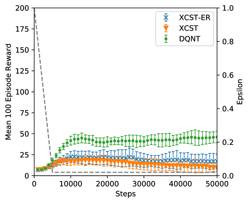
(d) XCST vs. XCST-ER in CartPole.

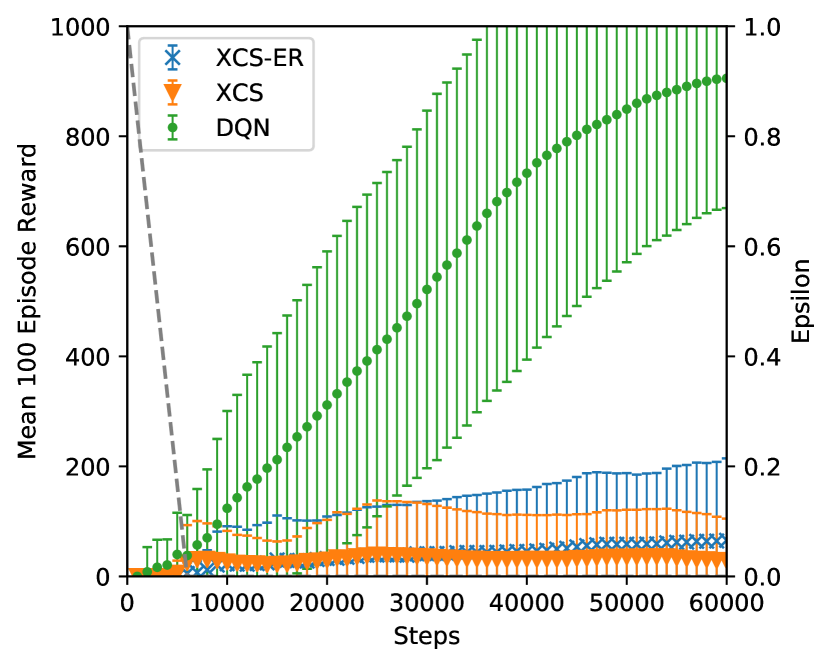
(e) XCS vs. XCS-ER in MountainCar.

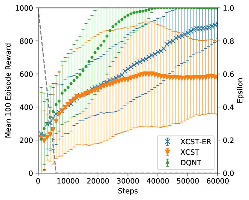
(f) XCST vs. XCST-ER in MountainCar.

Figure 2. XCS vs. XCS-ER vs. DQN on multi-step problems.

The observed results for the multi-step case reveal that ER amplifies a well-recognized issue of XCS when applied to sequential control tasks demanding for sustenance of long-action-chains – the occurrence of overgeneral classifiers bearing the risk of population divergence. Contrary to our initially posed hypothesis, ER aggravates this phenomenon by promoting misleading fitness signals through quicker convergence of the classifiers’ error estimates in spite of actually being overly general. Paired with XCS’s current deficiency in reliably identifying such actually inaccurate rules in turn fuels the employed GA which is responsible for seeking maximally general rules without loosing fitness (i.e., predictive accuracy). This problem becomes even more dramatic in problems with continuous state spaces, demanding for hyperrectangular condition representations. Due to the adapted mutation operations, a lack of pressure toward more specified rules exists in contrast to ternary coded classifier conditions (Butz et al., 2005).

Interestingly, throughout all experiments, DQN showed superior or at least similar performance compared to XCS with and without ER. So far, we did not fully understand the concrete reasons for that observation which prompts for further research in this direction.

6. Conclusion

We presented XCS-ER, an extended version of XCS which makes use of past experiences through an experience replay mechanism. A literature review revealed that the interest in combining LCS with memory mechanisms providing access to raw experiences not further fed into an internal model building process has been rather low. The reported results of conducted empirical studies promise that ER leads to significant improvements for single-step problems. In contrast, after setting multi-step problems in the spotlight, it turned out that ER bears the risk to dramatically aggravate already recognized issues inherent to XCS when confronted with learning tasks demanding for establishment of long-action-chains; a domain where RL-approaches such as DQN prove better suited so far.

Further research will be explicitly targeted at demystifying the not yet fully understood reasons for why DQN works so much better on difficult, i.e., long-action-chain demanding sequential control tasks such as MountainCar (see discussion above). Deeper investigations of XCS regarding its still prevalent overgeneralization issue in long-action-chain environments have to be conducted, comprising the combination of ER with countermeasures against overgeneralization such as the recently proposed absumption routine or the specify operator as introduced by Liu et al. (Liu et al., 2019) and Lanzi (Lanzi, 1999), respectively. As soon as the identified pitfalls of integrating ER in XCS for multi-step problems are understood more clearly, more sophisticated ER strategies such as Hindsight ER (Andrychowicz et al., 2017), Prioritized ER (Schaul et al., 2015), or a recently proposed interpolation-based technique for bootstrapping the replay memory (von Pilchau et al., 2020) will serve as subject for further improvements.

Appendix A Supplemental Material

A.1. Experiment Configurations

Environment Modifications

For the n-Chain environment, the episode length was reduced from 1000 to only 200, what increases the problem difficulty.

For the CartPole environment, the input parameters have been re-scaled to the interval [0,1] (using reasonable lower and upper bounds as determined in preliminary runs) since the utilized XCS implementation expects normalized inputs. The reward scheme was slightly modified to deliver +1 every time the pole keeps balanced by the cart and 0 if it has fallen. This provides a clearer reward signal and facilitates quicker learning for each of the compared algorithms.

Regarding the MountainCar environment, we again changed the episode length from 200 to 500, since both XCS variants encountered problems in randomly stumbling into the goal state within only 200 steps. Further, the reward scheme was made binary, i.e., instead of paying -1 for every step (includes reaching the terminal/goal state), we chose to apply a 0/1000 scheme. The latter only pays a reward of 1000 when reaching the goal, otherwise 0. This modification essentially increases the problem difficulty, since it renders the reward signal sparse.

Table 2. Configured hyperparameter settings. Abbreviations used: TS = tournament selection, UBR = unordered bound hyperrectangular representation, WH = Widrow-Hoff learning rule, RLS = recursive least square learning rule

Parameter	Mario	6-RMP	WBC	16chain	CartPole	M.Car
Learning steps	100k	40k	50k	50k	50k	60k
$N_{max}$	7000	800	6400	1000	5000	3000
$\beta$	0.3	0.2	0.2	0.1	0.1	0.1
$\gamma$	-	-	-	0.9	0.99	0.99
Fitness parameters:
$\alpha$	0.1	0.1	0.1	0.1	0.1	0.1
$\epsilon_{0}$	10	10	1	0.1	8.0	0.1
$\nu$	5	5	5	5	5	5
Deletion parameters:
$\theta_{del}$	50	20	50	20	200	200
$\delta$	0.1	0.1	0.1	0.1	0.1	0.1
Covering parameters:
$\theta_{mna}$	7	2	2	2	2	3
$p_{ini}$	10	10	10	10	0.01	0.01
$\epsilon_{ini}$	0	0	0	10	0.01	0.01
$F_{ini}$	0.01	0.01	0.01	0.01	0.01	0.01
GA parameters:
$\mu$	0.04	0.04	0.04	0.04	0.04	0.04
$\chi$	0.8	0.8	0.8	0.8	0.8	0.8
$\theta_{GA}$	30	12	48	50	25	50
$\theta_{sub}$	50	20	50	200	20	20
GA-selection	TS	TS	TS	TS	TS	TS
$F_{reduce}$	0.1	0.1	0.1	0.1	0.1	0.1
$\epsilon_{reduce}$	1.0	1.0	1.0	0.25	0.25	0.25
Condition parameters:
Condition	UBR	UBR	UBR	UBR	UBR	UBR
$m_{0}$	0.1	0.1	0.2	0.1	0.1	0.1
$r_{0}$	0.1	1.0	0.4	0.2	0.2	0.33
Prediction parameters:
Prediction	scalar	scalar	scalar	scalar	linear	linear
Learning rule	WH	WH	WH	WH	RLS	RLS
$\delta_{RLS}$	-	-	-	-	1.0	500
$\lambda_{RLS}$	-	-	-	-	1.0	1.0

For all experiments a maximum capacity for the Replay Memory (RM) of $N=50k$ has been chosen. The mini-batch size was set to $m=4$. In all experiments, a warm-up phase to fill the RM was conducted during the initial $1000$ steps. No learning happened in this phase.

A.2. Additional Statistics

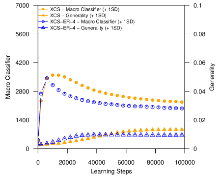
Figure 3. XCS vs. XCS-ER on Mario pixel art.

Table 3. Shapiro-Wilk tests for normality on the Mario problem. The resulting p-values are given in the cells. * (**) indicates a p-value ¡ $\alpha$ = 0.05 (0.01), i.e. a high likelihood that the null hypothesis (normality) can be rejected. p-values below 0.05 are marked in bold.

Mario	XCS-ER-8	XCS-ER-4	XCS
Reward mean	0.783	0.637	0.936
System error mean	0.467	0.858	0.065
Macroclassifiers mean	0.209	0.863	0.235
Generality mean	0.213	0.586	0.110

Table 4. Paired one-sided t-tests for XCS vs. XCS-ER on the Mario problem. The resulting p-values are given in the cells. * (**) indicates a p-value ¡ $\alpha$ = 0.05 (0.01), i.e. a high likelihood the deviation is statistically significant. p-values below 0.05 are marked in bold.

Mario	XCS-ER-8	XCS-ER-4
Reward mean	0.000**	0.000**
System error mean	0.000**	0.000**
Macroclassifiers mean	0.000**	0.000**
Generality mean	0.000**	0.000**

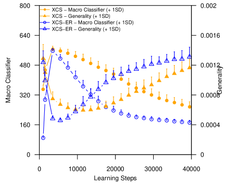
Figure 4. XCS vs. XCS-ER on 6-Real Multiplexer

Table 5. Shapiro-Wilk tests for normality for the 6-RMP problem. The resulting p-values are given in the cells. * (**) indicates a p-value ¡ $\alpha$ = 0.05 (0.01), i.e. a high likelihood that the null hypothesis (normality) can be rejected. p-values below 0.05 are marked in bold.

6-Real Multiplexer	XCS-ER	XCS
Reward mean	0.060	0.872
System error mean	0.143	0.714
Macroclassifiers mean	0.037*	0.882
Generality mean	0.846	0.117

Table 6. Paired one-sided t-tests for XCS vs. XCS-ER on the 6-RMP problem. The resulting p-values are given in the cells. * (**) indicates a p-value ¡ $\alpha$ = 0.05 (0.01), i.e. a high likelihood the deviation from the baseline (XCS without ER) is statistically significant. p-values below 0.05 are marked in bold.

6-Real Multiplexer	XCS-ER
Reward mean	0.000**
System error mean	0.000**
Macroclassifiers mean	0.000**
Generality mean	0.000**

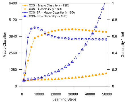
Figure 5. XCS vs. XCS-ER on WBC classification

Table 7. Shapiro-Wilk tests for normality on the WBC data set. The resulting p-values are depicted in the cells. * (**) indicates a p-value ¡ $\alpha$ = 0.05 (0.01), i.e. a high likelihood that the null hypothesis (normality) can be rejected. p-values below 0.05 are marked in bold.

WBC	XCS-ER	XCS
Reward mean	0.458	0.333
System error mean	0.195	0.316
Macroclassifiers mean	0.096	0.458
Generality mean	0.026*	0.003**

Table 8. Paired one-sided t-tests for XCS vs. XCS-ER on the WBC data set. The resulting p-values are given in the cells. * (**) indicates a p-value ¡ $\alpha$ = 0.05 (0.01), i.e. a high likelihood the deviation from the baseline (XCS without ER) is statistically significant. p-values below 0.05 are marked in bold.

WBC	XCS-ER
Reward mean	0.000**
System error mean	0.000**
Macroclassifiers mean	0.000**
Generality mean	0.000**

Table 9. Overall results for the multi-step environments: Reward, prediction error, population size in macroclassifiers, generality, OTM and Divergences are shown. Table entries indicate the overall means $\pm$1SD over the 30 repetitions. Divergence criteria for individual repetitions for 16Chain, CartPole, MountainCar are OTM values below 1, 70 and 200 respectively. ’T’ indicates active teletransportation. Arrows show whether the metric increased up or decreased. Statistical significance when compared to the regular XCS is determined via the Wilcoxon signed-rank test. * (**) indicates a p-value ¡ $\alpha$ = 0.05 (0.01). p-values below 0.05 confirming improvements are given in bold.

16Chain	Reward	Pr.Err.	$|[P]|$	Gen.	OTM	Div
XCS-ER	0.56$\downarrow$** $\pm$0.37	0.23$\uparrow$** $\pm$0.01	92.92$\downarrow$** $\pm$25.81	0.13$\uparrow$** $\pm$0.06	95.3$\downarrow$** $\pm$63.6	9$\uparrow$
DQN	n/a	n/a	n/a	n/a	143.1$\uparrow$ $\pm$1.4	0$\downarrow$
XCS	0.82 $\pm$0.15	0.14 $\pm$0.03	152.68 $\pm$22.16	0.07 $\pm$0.02	138.6 $\pm$25.7	1
16Chain T	Reward	Pr.Err.	$|[P]|$	Gen.	OTM	Div
XCST-ER	0.86$\downarrow$ $\pm$0.03	0.24$\uparrow$** $\pm$0.01	111.65$\downarrow$ $\pm$21.94	0.10$\uparrow$ $\pm$0.05	147.6$\downarrow$ $\pm$4.2	0
DQNT	n/a	n/a	n/a	n/a	148.0$\downarrow$ $\pm$5.8	0
XCST	0.88 $\pm$0.00	0.20 $\pm$0.03	117.90 $\pm$13.54	0.09 $\pm$0.01	149.2 $\pm$0.6	0
CartPole	Reward	Pr.Err.	$|[P]|$	Gen.	OTM	Div
XCS-ER	0.98$\downarrow$ $\pm$0.03	1.92$\uparrow$** $\pm$0.11	1937.44$\uparrow$** $\pm$106.85	0.0004$\uparrow$** $\pm$0.0000	93.0$\downarrow$ $\pm$47.6	9$\uparrow$
DQN	n/a	n/a	n/a	n/a	122.2$\uparrow$ $\pm$13.4	0$\downarrow$
XCS	0.99 $\pm$0.01	1.62 $\pm$0.25	1703.42 $\pm$161.46	0.0003 $\pm$0.0000	110.6 $\pm$46.5	7
CartPole T	Reward	Pr.Err.	$|[P]|$	Gen.	OTM	Div
XCST-ER	0.94$\uparrow$** $\pm$0.02	2.17$\uparrow$** $\pm$0.12	2162.30$\downarrow$** $\pm$51.94	0.0013$\uparrow$** $\pm$0.0000	18.29$\uparrow$** $\pm$6.22	30
DQNT	n/a	n/a	n/a	n/a	38.75** $\pm$2.19	30
XCST	0.92 $\pm$0.02	1.90 $\pm$0.09	2640.10 $\pm$70.37	0.0005 $\pm$0.0001	13.76 $\pm$3.59	30
M.Car	Reward	Pr.Err.	$|[P]|$	Gen.	OTM	Div
XCS-ER	0.13$\uparrow$ $\pm$0.06	1.73$\downarrow$** $\pm$2.77	383.25$\uparrow$ $\pm$204.68	0.05$\uparrow$** $\pm$0.01	38.57$\uparrow$ $\pm$86.37	29
DQN	n/a	n/a	n/a	n/a	504.96$\uparrow$** $\pm$216.03	3$\downarrow$
XCS	0.06 $\pm$0.15	3.5E5 $\pm$1.8E6	325.17 $\pm$162.39	0.04 $\pm$0.01	29.15 $\pm$63.27	29
M.Car T	Reward	Pr.Err.	$|[P]|$	Gen.	OTM	Div
XCST-ER	4.33$\uparrow$* $\pm$1.3	12.40$\downarrow$** $\pm$3.69	1150.36$\uparrow$ $\pm$88.24	0.01$\downarrow$** $\pm$0.00	626.3$\uparrow$ $\pm$132.4	0$\downarrow$
DQNT	n/a	n/a	n/a	n/a	814.5$\uparrow$** $\pm$90.9	0$\downarrow$
XCST	3.22 $\pm$2.17	1.2E21 $\pm$6.3E21	1041.51 $\pm$114.82	0.02 $\pm$0.00	511.2 $\pm$219.5	5

Table 10. Shapiro-Wilk tests for normality on the multi-step environments. The resulting p-values are given in the cells. * (**) indicates a p-value ¡ $\alpha$ = 0.05 (0.01), i.e. a high likelihood that the null hypothesis (normality) can be rejected. p-values below 0.05 are marked in bold.

16Chain	XCS-ER	XCS	DQN
Reward mean	0.000**	0.000**	n/a
Prediction error mean	0.003**	0.366	n/a
Macroclassifiers mean	0.058	0.008**	n/a
Generality mean	0.000**	0.000**	n/a
OTM	0.000**	0.000**	0.000**
16Chain Tele.	XCS-ER	XCS	DQN
Reward mean	0.000**	0.037*	n/a
Prediction error mean	0.001**	0.531	n/a
Macroclassifiers mean	0.000**	0.597	n/a
Generality mean	0.000**	0.733	n/a
OTM	0.000**	0.02*	0.000**
CartPole	XCS-ER	XCS	DQN
Reward mean	0.000**	0.000**	n/a
Prediction error mean	0.625	0.023*	n/a
Macroclassifiers mean	0.875	0.222	n/a
Generality mean	0.432	0.618	n/a
OTM	0.006**	0.000**	0.099
CartPole Tele.	XCS-ER	XCS	DQN
Reward mean	0.056	0.639	n/a
Prediction error mean	0.184	0.167	n/a
Macroclassifiers mean	0.026*	0.976	n/a
Generality mean	0.594	0.240	n/a
OTM	0.177	0.002**	0.370
MountainCar	XCS-ER	XCS	DQN
Reward mean	0.000**	0.000**	n/a
Prediction error mean	0.000**	0.000**	n/a
Macroclassifiers mean	0.000**	0.006**	n/a
Generality mean	0.367	0.303	n/a
OTM	0.000**	0.000**	0.023*
MountainCar Tele.	XCS-ER	XCS	DQN
Reward mean	0.673	0.067	n/a
Prediction error mean	0.641	0.000**	n/a
Macroclassifiers mean	0.024*	0.023*	n/a
Generality mean	0.070	0.000**	n/a
OTM	0.004**	0.042	0.005**

As can be noticed, most of the metrics do not follow a normal distribution. Even if normality can be confirmed in certain cases, a parametric test is still not plausibly applicable when the sample considered for comparison violates this assumption. For that reason, we decided to exclusively conduct non-parametric Wilcoxon tests across all multi-step experiments.

Table 11. Wilcoxon signed-rank tests for the multi-step environments. The resulting p-values are given in the cells. * (**) indicates a p-value ¡ $\alpha$ = 0.05 (0.01), i.e. a high likelihood that the deviation from the baseline (XCS without ER) is statistically significant. p-values below 0.05 are marked in bold.

16Chain	XCS-ER	DQN
Reward mean	0.000**	n/a
Prediction error mean	0.000**	n/a
Macroclassifiers mean	0.000**	n/a
Generality mean	0.000**	n/a
OTM	0.000**	0.959
16Chain Tele.	XCS-ER	DQN
Reward mean	0.254	n/a
Prediction error mean	0.000**	n/a
Macroclassifiers mean	0.349	n/a
Generality mean	0.644	n/a
OTM	0.394	0.504
CartPole	XCS-ER	DQN
Reward mean	0.136	n/a
Prediction error mean	0.000**	n/a
Macroclassifiers mean	0.000**	n/a
Generality mean	0.000**	n/a
OTM	0.111	0.428
CartPole Tele.	XCS-ER	DQN
Reward mean	0.000**	n/a
Prediction error mean	0.000**	n/a
Macroclassifiers mean	0.000**	n/a
Generality mean	0.000**	n/a
OTM	0.000**	0.000**
MountainCar	XCS-ER	DQN
Reward mean	0.178	n/a
Prediction error mean	0.002**	n/a
Macroclassifiers mean	0.360	n/a
Generality mean	0.001**	n/a
OTM	0.550	0.000**
MountainCar Tele.	XCS-ER	DQN
Reward mean	0.014*	n/a
Prediction error mean	0.000**	n/a
Macroclassifiers mean	0.000**	n/a
Generality mean	0.000**	n/a
OTM	0.060	0.000**

References

- (1)
- Andrychowicz et al. (2017) Marcin Andrychowicz, Filip Wolski, Alex Ray, Jonas Schneider, Rachel Fong, Peter Welinder, Bob McGrew, Josh Tobin, OpenAI Pieter Abbeel, and Wojciech Zaremba. 2017. Hindsight experience replay. In Advances in neural information processing systems. 5048–5058.
- Bacardit et al. (2009) Jaume Bacardit, Edmund K. Burke, and Natalio Krasnogor. 2009. Improving the scalability of rule-based evolutionary learning. Memetic Computing 1, 1 (01 Mar 2009), 55–67. https://doi.org/10.1007/s12293-008-0005-4
- Barry (2002) Alwyn Barry. 2002. The stability of long action chains in XCS. Soft Comput. 6, 3-4 (2002), 183–199. https://doi.org/10.1007/s005000100115
- Bernadó-Mansilla and Garrell-Guiu (2003) E. Bernadó-Mansilla and J. M. Garrell-Guiu. 2003. Accuracy-Based Learning Classifier Systems: Models, Analysis and Applications to Classification Tasks. Evolutionary Computation 11, 3 (Sept 2003), 209–238. https://doi.org/10.1162/106365603322365289
- Brockman et al. (2016) Greg Brockman, Vicki Cheung, Ludwig Pettersson, Jonas Schneider, John Schulman, Jie Tang, and Wojciech Zaremba. 2016. OpenAI Gym. arXiv:arXiv:1606.01540
- Bull et al. (2004) L. Bull, J. Sha’Aban, A. Tomlinson, J.D. Addison, and B.G. Heydecker. 2004. Towards Distributed Adaptive Control for Road Traffic Junction Signals using Learning Classifier Systems. In Applications of Learning Classifier Systems, Larry Bull (Ed.). Studies in Fuzziness and Soft Computing, Vol. 150. Springer Berlin Heidelberg, 276–299.
- Butz et al. (2005) M.V. Butz, D.E. Goldberg, and P.L. Lanzi. 2005. Gradient descent methods in learning classifier systems: improving XCS performance in multistep problems. Evolutionary Computation, IEEE Transactions on 9, 5 (Oct 2005), 452–473. https://doi.org/10.1109/TEVC.2005.850265
- Butz et al. (2008) M.V. Butz, P.L. Lanzi, and S.W. Wilson. 2008. Function Approximation With XCS: Hyperellipsoidal Conditions, Recursive Least Squares, and Compaction. Evolutionary Computation, IEEE Transactions on 12, 3 (June 2008), 355–376. https://doi.org/10.1109/TEVC.2007.903551
- Butz and Stolzmann (1999) M. Butz and W. Stolzmann. 1999. Action-Planning in Anticipatory Classifier Systems. In Proceedings of the 1999 Genetic and Evolutionary Computation Conference Workshop Program. 242–249.
- Butz and Stolzmann (2001) M.V. Butz and W. Stolzmann. 2001. An Algorithmic Description of ACS2. In International Workshop on Learning Classifier Systems. Springer, 211–229.
- Butz and Wilson (2002) M.V. Butz and S.W. Wilson. 2002. An Algorithmic Description of XCS. Soft Computing 6, 3-4 (2002), 144–153.
- Cliff and Ross (1994) Dave Cliff and Susi Ross. 1994. Adding Temporary Memory to ZCS. Adaptive Behavior 3, 2 (1994), 101–150. https://doi.org/10.1177/105971239400300201
- Gerard et al. (2002) P. Gerard, W. Stolzmann, and O. Sigaud. 2002. YACS: A new Learning Classifier System using Anticipation. Soft Computing 6, 3-4 (2002), 216–228.
- Holland (1986) John H. Holland. 1986. Escaping Brittleness: The Possibilities of General-Purpose Learning Algorithms Applied to Parallel Rule-Based Systems. In Machine Learning: An Artificial Intelligence Approach, R. S. Michalski, J. G. Carbonell, and T. M. Mitchell (Eds.). Vol. 2. Morgan Kaufmann, Los Altos, CA.
- Holland and Reitman (1978) J. H. Holland and J. S. Reitman. 1978. Cognitive Systems Based on Adaptive Algorithms. In Pattern directed inference systems, D. A. Waterman and F. Hayes-Roth (Eds.). Academic Press, New York, 313–329.
- Kharbat et al. (2008) Faten Kharbat, Mohammed Odeh, and Larry Bull. 2008. Knowledge Discovery from Medical Data: An Empirical Study with XCS. In Learning Classifier Systems in Data Mining, Larry Bull, Ester Bernadó-Mansilla, and John Holmes (Eds.). Studies in Computational Intelligence, Vol. 125. Springer Berlin Heidelberg, 93–121. https://doi.org/10.1007/978-3-540-78979-6_5
- Kovacs (2000) Tim Kovacs. 2000. Strength or Accuracy? Fitness Calculation in Learning Classifier Systems. Springer Berlin Heidelberg, Berlin, Heidelberg, 143–160. https://doi.org/10.1007/3-540-45027-0_7
- Lanzi (1998) P. L. Lanzi. 1998. Adding memory to XCS. In 1998 IEEE International Conference on Evolutionary Computation Proceedings. IEEE World Congress on Computational Intelligence (Cat. No.98TH8360). 609–614. https://doi.org/10.1109/ICEC.1998.700098
- Lanzi (1999) Pier Luca Lanzi. 1999. An analysis of generalization in the XCS classifier system. Evolutionary computation 7, 2 (1999), 125–149.
- Lanzi (2002) P. L. Lanzi. 2002. Learning classifier systems from a reinforcement learning perspective. Soft Computing 6, 3 (01 Jun 2002), 162–170. https://doi.org/10.1007/s005000100113
- Lanzi and Wilson (2000) Pier Luca Lanzi and Stewart W Wilson. 2000. Toward optimal classifier system performance in non-Markov environments. Evolutionary Computation 8, 4 (2000), 393–418.
- Lichman (2013) M. Lichman. 2013. UCI Machine Learning Repository. http://archive.ics.uci.edu/ml University of California, Irvine, School of Information and Computer Sciences, http://archive.ics.uci.edu/ml.
- Lin (1992) L. Lin. 1992. Self-improving Reactive Agents based on Reinforcement Learning, Planning and Teaching. Machine learning 8, 3-4 (1992), 293–321.
- Liu et al. (2019) Yi Liu, Will N. Browne, and Bing Xue. 2019. Absumption to Complement Subsumption in Learning Classifier Systems. In Proceedings of the Genetic and Evolutionary Computation Conference (GECCO ’19). Association for Computing Machinery, New York, NY, USA, 410–418. https://doi.org/10.1145/3321707.3321719
- Mnih et al. (2013) Volodymyr Mnih, Koray Kavukcuoglu, David Silver, Alex Graves, Ioannis Antonoglou, Daan Wierstra, and Martin Riedmiller. 2013. Playing atari with deep reinforcement learning. arXiv preprint arXiv:1312.5602 (2013). https://arxiv.org/pdf/1312.5602.pdf
- Mnih et al. (2015) Volodymyr Mnih, Koray Kavukcuoglu, David Silver, Andrei A. Rusu, Joel Veness, Marc G. Bellemare, Alex Graves, Martin Riedmiller, Andreas K. Fidjeland, Georg Ostrovski, Stig Petersen, Charles Beattie, Amir Sadik, Ioannis Antonoglou, Helen King, Dharshan Kumaran, Daan Wierstra, Shane Legg, and Demis Hassabis. 2015. Human-level control through deep reinforcement learning. Nature 518, 7540 (Feb. 2015), 529–533. http://dx.doi.org/10.1038/nature14236
- Nakata et al. (2017) Masaya Nakata, Will N. Browne, Tomoki Hamagami, and Keiki Takadama. 2017. Theoretical XCS parameter settings of learning accurate classifiers. In Proceedings of the Genetic and Evolutionary Computation Conference, GECCO 2017, Berlin, Germany, July 15-19, 2017. 473–480.
- Pätzel et al. (2019) David Pätzel, Anthony Stein, and Jörg Hähner. 2019. A Survey of Formal Theoretical Advances Regarding XCS. In Proceedings of the Genetic and Evolutionary Computation Conference Companion (GECCO ’19). ACM, New York, NY, USA, 1295–1302. https://doi.org/10.1145/3319619.3326848
- Pickering and Kovacs (2015) T. Pickering and T. Kovacs. 2015. TP-XCS: An XCS classifier system with fixed-length memory for reinforcement learning. In 2015 IEEE Congress on Evolutionary Computation (CEC). 3020–3025. https://doi.org/10.1109/CEC.2015.7257265
- Preen et al. (2019) Richard J. Preen, Stewart W. Wilson, and Larry Bull. 2019. Autoencoding with XCSF. arXiv:cs.NE/1910.10579
- Schaul et al. (2015) Tom Schaul, John Quan, Ioannis Antonoglou, and David Silver. 2015. Prioritized experience replay. arXiv preprint arXiv:1511.05952 (2015).
- Silver et al. (2017) David Silver, Julian Schrittwieser, Karen Simonyan, Ioannis Antonoglou, Aja Huang, Arthur Guez, Thomas Hubert, Lucas Baker, Matthew Lai, Adrian Bolton, Yutian Chen, Timothy Lillicrap, Fan Hui, Laurent Sifre, George Driessche, Thore Graepel, and Demis Hassabis. 2017. Mastering the game of Go without human knowledge. Nature 550 (10 2017), 354–359. https://doi.org/10.1038/nature24270
- Smith (1980) Stephen Frederick Smith. 1980. A Learning System Based on Genetic Adaptive Algorithms. Ph.D. Dissertation. Pittsburgh, PA, USA. AAI8112638.
- Stein et al. (2016a) Anthony Stein, Christian Eymüller, Dominik Rauh, Sven Tomforde, and Jörg Hähner. 2016a. Interpolation-based Classifier Generation in XCSF. In Proceedings of 2016 IEEE Congress on Evolutionary Computation (CEC). IEEE, 3990–3998.
- Stein et al. (2017a) Anthony Stein, Roland Maier, and Jörg Hähner. 2017a. Toward Curious Learning Classifier Systems: Combining XCS with Active Learning Concepts. In Proceedings of the Genetic and Evolutionary Computation Conference (GECCO) Companion. ACM, 1349–1356.
- Stein et al. (2018) Anthony Stein, Simon Menssen, and Jörg Hähner. 2018. What About Interpolation? A Radial Basis Function Approach to Classifier Prediction Modeling in XCSF. In Proceedings of the Genetic and Evolutionary Computation Conference (GECCO). ACM, New York, NY, USA, 537–544.
- Stein et al. (2016b) Anthony Stein, Dominik Rauh, Sven Tomforde, and Jörg Hähner. 2016b. Augmenting the Algorithmic Structure of XCS by Means of Interpolation. In Proceedings of 29th International Conference on Architecture of Computing Systems (ARCS). Springer International Publishing, 348–360.
- Stein et al. (2017b) Anthony Stein, Dominik Rauh, Sven Tomforde, and Jörg Hähner. 2017b. Interpolation in the eXtended Classifier System: An architectural perspective. Journal of Systems Architecture 75 (2017), 79 – 94. https://doi.org/10.1016/j.sysarc.2017.01.010
- Stein et al. (2017c) Anthony Stein, Stefan Rudolph, Sven Tomforde, and Jörg Hähner. 2017c. Self-Learning Smart Cameras – Harnessing the Generalization Capability of XCS. In Proceedings of International Joint Conference on Computational Intelligence IJCCI 2017. Funchal, Madeira - Portugal, 129 – 140.
- Stolzmann (1998) W. Stolzmann. 1998. Anticipatory Classifier Systems. Genetic Programming 98 (1998), 658–664.
- Stone and Bull (2003) Christopher Stone and Larry Bull. 2003. For Real! XCS with Continuous-Valued Inputs. Evolutionary Computation 11, 3 (2003), 298–336.
- Strens (2000) Malcolm J. A. Strens. 2000. A Bayesian Framework for Reinforcement Learning. In Proceedings of the Seventeenth International Conference on Machine Learning (ICML ’00). Morgan Kaufmann Publishers Inc., San Francisco, CA, USA, 943–950.
- Sutton (1991) R.S. Sutton. 1991. Dyna, an integrated Architecture for Learning, Planning, and Reacting. ACM SIGART Bulletin 2, 4 (1991), 160–163.
- Sutton and Barto (1998) Richard S. Sutton and Andrew G. Barto. 1998. Reinforcement Learning: An Introduction. MIT Press. http://www.cs.ualberta.ca/~sutton/book/the-book.html
- Tamee et al. (2007) Kreangsak Tamee, Larry Bull, and Ouen Pinngern. 2007. Towards Clustering with XCS. In Proceedings of the 9th Annual Conference on Genetic and Evolutionary Computation (GECCO ’07). ACM, New York, NY, USA, 1854–1860. https://doi.org/10.1145/1276958.1277326
- Tsitsiklis and Van Roy (1997) J. N. Tsitsiklis and B. Van Roy. 1997. An analysis of temporal-difference learning with function approximation. IEEE Trans. Automat. Control 42, 5 (May 1997), 674–690. https://doi.org/10.1109/9.580874
- Urbanowicz et al. (2014) Ryan J. Urbanowicz, Gediminas Bertasius, and Jason H. Moore. 2014. An Extended Michigan-Style Learning Classifier System for Flexible Supervised Learning, Classification, and Data Mining. In Parallel Problem Solving from Nature – PPSN XIII, Thomas Bartz-Beielstein, Jürgen Branke, Bogdan Filipič, and Jim Smith (Eds.). Springer International Publishing, Cham, 211–221.
- Urbanowicz and Moore (2015) Ryan J. Urbanowicz and Jason H. Moore. 2015. ExSTraCS 2.0: description and evaluation of a scalable learning classifier system. Evolutionary Intelligence 8, 2 (2015), 89–116. https://doi.org/10.1007/s12065-015-0128-8
- Vinyals et al. (2019) Oriol Vinyals, Igor Babuschkin, Wojciech M Czarnecki, Michaël Mathieu, Andrew Dudzik, Junyoung Chung, David H Choi, Richard Powell, Timo Ewalds, Petko Georgiev, Junhyuk Oh, Dan Horgan, Manuel Kroiss, Ivo Danihelka, Aja Huang, Laurent Sifre, Trevor Cai, John P Agapiou, Max Jaderberg, Alexander S Vezhnevets, Rémi Leblond, Tobias Pohlen, Valentin Dalibard, David Budden, Yury Sulsky, James Molloy, Tom L Paine, Caglar Gulcehre, Ziyu Wang, Tobias Pfaff, Yuhuai Wu, Roman Ring, Dani Yogatama, Dario Wünsch, Katrina McKinney, Oliver Smith, Tom Schaul, Timothy Lillicrap, Koray Kavukcuoglu, Demis Hassabis, Chris Apps, and David Silver. 2019. Grandmaster level in StarCraft II using multi-agent reinforcement learning. Nature 575, 7782 (2019), 350–354. https://doi.org/10.1038/s41586-019-1724-z
- von Pilchau et al. (2020) Wenzel Baron Pilar von Pilchau, Anthony Stein, and Jörg Hähner. 2020. Bootstrapping a DQN Replay Memory with Synthetic Experiences. arXiv:cs.LG/2002.01370
- Watkins (1989) Christopher John Cornish Hellaby Watkins. 1989. Learning from Delayed Rewards. Ph.D. Dissertation. King’s College, Cambridge, UK. http://www.cs.rhul.ac.uk/~chrisw/new_thesis.pdf
- Wilson (1994) Stewart W. Wilson. 1994. ZCS: A Zeroth Level Classifier System. Evolutionary Computation 2, 1 (1994), 1–18.
- Wilson (1995) Stewart W. Wilson. 1995. Classifier Fitness Based on Accuracy. Evolutionary computation 3, 2 (1995), 149–175.
- Wilson (1998) Stewart W. Wilson. 1998. Generalization in the XCS Classifier System. Genetic Programming 1998 : Proceedings of the Third Annual Conference (1998).
- Wilson (2000) Stewart W. Wilson. 2000. Get Real! XCS with Continuous-Valued Inputss. In Learning Classifier Systems, Pier Luca Lanzi, Wolfgang Stolzmann, and Stewart W. Wilson (Eds.). Lecture Notes in Computer Science, Vol. 1813. Springer Berlin Heidelberg, 209–219. https://doi.org/10.1007/3-540-45027-0_11
- Wilson (2001) Stewart W. Wilson. 2001. Mining Oblique Data with XCS. In Advances in learning classifier systems: Third international workshop, IWLCS 2000 (LNAI 1996), P. L. Lanzi, W. Stolzmann, and Stewart W. Wilson (Eds.). Springer-Verlag, Berlin Heidelberg, 158–174.