An explicit algebraic closure for passive scalar-flux: Applications in heated channel flows subjected to system rotation

Abstract

We present an algebraic model for turbulent scalar-flux vector that stems from tensor representation theory. The resulting closure contains direct dependence on mean velocity gradients and on frame rotation tensor that accounts for Coriolis effects. Model coefficients are determined from Direct Numerical Simulations (DNS) data of homogeneous shear flows subjected to arbitrary mean scalar gradient orientations. This type of tuning process renders the proposed model to be objective towards inhomogeneous applications. Model performance is evaluated in several heated channel flows in both stationary and rotating frames, showing good results. To place the performance of the proposed model into context, we compare with Younis algebraic model [1], which is known to provide reasonable predictions for several engineering flows.

1 INTRODUCTION

Turbulent scalar-flux vector has a notable role in the scalar transport for a wide range of practical applications. It appears in the Reynolds-Averaged scalar transport equations as a term that needs to be modelled so that closure is achieved. An elegant choice is the development of engineering models with aim to provide estimations of this quantity at low computational complexity. Engineering models for the scalar-flux are classified into two categories: differential and algebraic. Differential transport models (DTM) are proven to be beneficial tools, being capable of handling rotational and curvature effects. However, robustness issues and performance inconsistencies, combined with computational overheads associated with the solution of a differential transport equation for each scalar-flux component, prevent this class of models from penetrating further into the mainstream of engineering practice. On the other hand, algebraic approaches are based on assumptions that lead to constitutive equations between turbulent statistics and mean deformation. The simplest algebraic model is based on the gradient-diffusion hypothesis (GDH), which assumes that turbulent scalar-flux is aligned to the mean scalar gradient. Despite its implementational and computational elegance, this assumption is an important reason why this model fails to capture important flow features, such as turbulence anisotropy or the effects of mean and system rotation. As a result, Batchelor [2] proposed a generalization of GDH (GGDH) from which several algebraic closures have emerged. For example, Daly $\&$ Harlow [3] adopted scale functions to express the turbulent scalar-flux vector as a product between Reynolds stress and mean scalar-gradient, allowing the mis-alignment of the scalar-fluxes with the mean scalar deformation. However, this expression is found to perform poorly on predicting the correct magnitudes of scalar-flux components in the directions normal to the mean scalar gradient. Suga $\&$ Abe [4] improved the performance of the GGDH model by adding a non-linear term that contains quadratic products of the Reynolds stress tensor, which correctly captures the anisotropy levels of the scalar-flux components in the vicinity of wall boundaries. This addition resulted in the construction of Higher-Order GGDH models (HO-GGDH), which were successfully applied in a wide range of heated channel flows. Another interesting approach is to derive algebraic expressions directly from the exact transport equation of turbulent scalar-flux through equilibrium assumptions. A common choice is to apply the weak-equilibrium assumption (WEA) [5], which states that the transient variations of turbulent anisotropies are negligible compared to the variation of turbulent scales. To some extent, these models are considered to be a good alternative to DTM, as they have been successfully applied in different flow configurations while requiring less computational capacity [6, 7, 8].

An alternative approach for estimating the turbulent scalar-fluxes was proposed by Younis et al. [9]. Using as guidance the exact scalar-flux transport equation, Younis and coworkers expressed this quantity as a function of several tensor quantities. This approach is elegant, since it avoids the reduction of transport equations through the WEA with all the modelling uncertainties that entails. It also provides a general framework, from which different algebraic expressions can be obtained. They proposed a multi-linear closure that exhibited distinct improvements over other algebraic scalar-flux closures in benchmark two-dimensional free shear flows, while it was successfully used in flow configurations involving Coriolis and curvature effects [10, 11]. However, the linear nature of this specific closure is the main reason why it fails to capture the proper near-wall anisotropy levels of scalar-flux vector, thus revealing the importance of incorporating non-linear information regarding turbulence anisotropy. Hence, in this study we propose an algebraic model that stems directly from the Younis formulation and involves products of the Reynolds stress tensor, a dependence missing from the multi-linear model. Special attention is given so that model complexity is kept minimal for ease implementation in existing industrial codes, while its performance ability is tested on several heated Couette and Poiseuille flows in stationary and rotating frames.

A description of the exact transport equations of the turbulent passive-scalar fluxes along with an extensive summary of the Younis approach are given in Section 2 with the motivation behind the use of a non-linear term involving products of Reynolds stress given in Section 3. The proposed formulation is discussed in Section 4 and the performance of this closure is evaluated in Section 5, yielding good results. Summary and conclusions are given in Section 6.

2 YOUNIS’ FORMULATION

The motivation behind the work reported by Younis et al. [9] arose from the need to provide a better alternative to the existing gradient-transport closures for the turbulent scalar-fluxes. As starting point, they considered the exact transport equation of these fluxes in a frame rotating at a constant angular velocity rate $\Omega^{f}$

$$\begin{split}\frac{\partial\overline{u^{\prime}_{i}\phi^{\prime}}}{\partial t}+\overline{u}_{j}\frac{\partial\overline{u^{\prime}_{i}\phi^{\prime}}}{\partial x_{j}}=&-\overline{u^{\prime}_{i}u^{\prime}_{j}}\frac{\partial\overline{\phi}}{\partial x_{j}}-\overline{u^{\prime}_{j}\phi^{\prime}}\frac{\partial\overline{u}_{i}}{\partial x_{j}}-2\epsilon_{ijk}\Omega^{f}_{j}\overline{u^{\prime}_{k}\phi^{\prime}}\\ &-\frac{1}{\rho}\overline{p^{\prime}\frac{\partial\phi^{\prime}}{\partial x_{i}}}-(\gamma+\nu)\overline{\frac{\partial\phi^{\prime}}{\partial x_{j}}\frac{\partial u^{\prime}_{i}}{\partial x_{j}}}\\ &-\frac{\partial}{\partial x_{j}}\bigg{(}\overline{u^{\prime}_{i}u^{\prime}_{j}\phi^{\prime}}+\frac{1}{\rho}\overline{p^{\prime}\phi^{\prime}}\delta_{ij}-\gamma\overline{u^{\prime}_{i}\frac{\partial\phi^{\prime}}{\partial x_{j}}}-\nu\overline{\phi^{\prime}\frac{\partial u^{\prime}_{i}}{\partial x_{j}}}\bigg{)}\,,\end{split}$$ (1)

where the instantaneous flow variables are decomposed into a mean part, denoted by overbar, and a fluctuating part, denoted by prime symbol. Hereafter, we are using index notation whereby repeated indexes imply summation. The coefficient of fluid viscosity and the coefficient of scalar diffusivity are denoted by $\nu$ and $\gamma$ respectively, $\rho$ is the density of the fluid and $u_{i}$, $\phi$ are the instantaneous fluid velocity and passive scalar fields respectively. The fluctuating pressure is denoted with $p^{\prime}$. The first and second terms on the RHS of equation (1) represent the generation of scalar-flux as a consequence of turbulence-mean deformation interactions. The third term arises when flow is subjected to system rotation around an arbitrary axis, while the fourth term refers to the fluctuating pressure-scalar correlations and is responsible for the redistribution of the flux among the different components. The fifth term refers to the rate at which the scalar-flux is destructed, while the last term is interpreted as the turbulent-transport term. Younis et al. [9] used equation (1) as a guide to provide a rationally assumed relationship between the scalar-flux vector and various tensor quantities,

$$\overline{u^{\prime}_{i}\phi^{\prime}}=f_{i}\bigg{(}R_{ij},S_{ij},W_{ij},\Omega^{f}_{ij},\Lambda_{i},\epsilon,\epsilon_{\phi},\overline{\phi^{{}^{\prime}2}}\bigg{)}\,,$$ (2)

where $R_{ij}=\overline{u^{\prime}_{i}u^{\prime}_{j}}$ is the Reynolds stress tensor, $\epsilon$ is the energy dissipation rate, $\epsilon_{\phi}$ is half the scalar dissipation rate and $\overline{\phi^{{}^{\prime}2}}$ is the scalar-variance. $S_{ij}$, $W_{ij}$, $\Omega^{f}_{ij}$ and $\Lambda_{i}$ denote the mean strain-rate tensor, the mean vorticity tensor, the frame-rotation rate tensor and the mean scalar gradient vector respectively, defined as

$$\begin{split}S_{ij}&=\frac{1}{2}\bigg{(}\frac{\partial\overline{u}_{i}}{\partial x_{j}}+\frac{\partial\overline{u}_{j}}{\partial x_{i}}\bigg{)}\,,\qquad W_{ij}=\frac{1}{2}\bigg{(}\frac{\partial\overline{u}_{i}}{\partial x_{j}}-\frac{\partial\overline{u}_{j}}{\partial x_{i}}\bigg{)}\,,\qquad\Omega^{f}_{ij}=\epsilon_{ikj}\,\Omega^{f}_{k}\,,\qquad\Lambda_{i}=\frac{\partial\overline{\phi}}{\partial x_{i}}\,.\end{split}$$ (3)

With the aid of tensor representation theory, Younis et al. constructed an explicit model for $\overline{u^{\prime}_{i}\phi^{\prime}}$ in accordance with equation (2). Under this approach, $\overline{u^{\prime}_{i}\phi^{\prime}}$ can be expressed as a series of basis vectors $\Upsilon_{i}$,

$$\overline{u^{\prime}_{i}\phi^{\prime}}=\sum^{M}_{n=1}\alpha_{n}\Upsilon^{n}_{i}\,,$$ (4)

where $\alpha_{n}$ can depend on all the tensor variables appearing in equation (2). The basis vectors are formed from the products of the symmetric ($S_{ij},R_{ij}$), the skew-symmetric ($W_{ij}$) tensors and the vector ($\Lambda_{i}$), leading to the following algebraic expression

$$\begin{split}\overline{u^{\prime}_{i}\phi^{\prime}}&=\alpha_{1}\Lambda_{i}+\alpha_{2}R_{ij}\Lambda_{j}+\alpha_{3}S_{ij}\Lambda_{j}+\alpha_{4}R_{ik}R_{kj}\Lambda_{j}+\alpha_{5}S_{ik}S_{kj}\Lambda_{j}+\alpha_{6}W_{ij}\Lambda_{j}\\ &+\alpha_{7}W_{ik}W_{kj}\Lambda_{j}+\alpha_{8}\bigg{(}S_{ik}W_{kj}+S_{jk}W_{ki}\bigg{)}\Lambda_{j}+\alpha_{9}\bigg{(}R_{ik}S_{kj}+R_{jk}S_{ki}\bigg{)}\Lambda_{j}\\ &+\alpha_{10}\bigg{(}R_{ik}W_{kj}+R_{jk}W_{ki}\bigg{)}\Lambda_{j}\,,\end{split}$$ (5)

where for simplicity we neglected the presence of Coriolis effects in the above expression. To bring the above expression into a more compact form, Younis et al. [9] assumed sufficiently small anisotropies and turbulent time scales. Further assuming that the effects of $S_{ij}$ and $W_{ij}$ are in balance, results to the following multilinear expression:

$$\overline{u^{\prime}_{i}\phi^{\prime}}=C_{1}\frac{\kappa^{2}}{\epsilon}\Lambda_{i}+C_{2}\frac{\kappa}{\epsilon}R_{ij}\Lambda_{j}+C_{3}\frac{\kappa^{3}}{\epsilon^{2}}G^{T}_{ij}\Lambda_{j}+C_{4}\frac{\kappa^{2}}{\epsilon^{2}}\bigg{(}R_{ik}G^{T}_{jk}+R_{jk}G^{T}_{ik}\bigg{)}\Lambda_{j}\,,\qquad G^{T}_{ij}=G_{ij}+\Omega^{f}_{ij}\,,$$ (6)

where $\kappa=R_{kk}/2$ is the turbulent kinetic energy, while the $\alpha_{i}$ coefficients were replaced based on dimensional arguments. Coriolis effects are explicitly incorporated in the closure by adding the frame-rotation tensor $\Omega^{f}_{ij}$ into the mean velocity gradient tensor $G_{ij}=S_{ij}+W_{ij}$, an approach also followed in previous studies [12]. The first term on the RHS of equation (6) represents the GDH, while the second term coincides with the production term that appears in equation (1) and is associated with the mean scalar deformation, also known as the Generalized Gradient Diffusion Hypothesis (GGDH) model proposed by Daly $\&$ Harlow [3]. The remaining two terms involve products between the gradients of mean scalar and mean velocity; a dependence proposed by the analyses of Dakos $\&$ Gibson [13] and Yoshizawa [14]. The values of $C_{i}$ coefficients were determined based on the LES results of Kaltenbach [15] for homogeneous flows subjected to a uniform shear with uniform scalar gradients

$$C_{1}=0.0455\,,\qquad C_{2}=-0.373\,,\qquad C_{3}=0.00373\,,\qquad C_{4}=0.0235\,.$$ (7)

Regarding inhomogeneous flows, detailed analysis of the model performance in relation to data from a large number of studies on wall-bounded flows showed a serious error in the normal flux component [10]. As a result, the value of $C_{1}$ coefficient was modified in the near-wall region by applying the following damping function

$$C_{1}=0.0455\,f_{C_{1}},\qquad f_{C1}=1-\exp(-A\,\beta\,Pe^{\alpha}),\qquad Pe=Pr\,Re_{\tau}\,,$$ (8)

where $\alpha=-0.02$ and $\beta=1.9$ are the values proposed by Younis et al. [1], $Pr=\nu/\gamma$ is the Prandtl number, $Re_{t}=\frac{\kappa^{2}}{\nu\epsilon}$ is the turbulence Reynolds number, while $A$ is the stress-flatness parameter, defined as

$$\begin{split}A_{ij}&=\frac{R_{ij}}{\kappa}-\frac{2}{3}\delta_{ij}\,,\qquad A_{2}=A_{ij}A_{ji}\,,\qquad A_{3}=A_{ij}A_{jk}A_{ki}\,,\qquad A=1-\frac{9}{8}(A_{2}-A_{3})\,,\end{split}$$ (9)

where $A_{2}$ and $A_{3}$ are the second and third invariants of the normalized Reynolds-stress anisotropic tensor $A_{ij}$. More details regarding the mathematical formulation can be found in Younis et al. [10].

As already mentioned in the introduction, the linear form of Younis closure is an important reason why this closure exhibits certain limitations. For example, it fails to capture the near-wall anisotropy levels of the scalar-flux vector. In the following section we discuss the importance of incorporating a term that contains non-linear information regarding the turbulent anisotropy, vital to predict the proper near-wall behaviour.

3 QUADRATIC DEPENDENCE ON REYNOLDS STRESS

It is well known that models involving only the second term of equation (6) cannot predict the streamwise heat-flux component reasonably well [16]. In an attempt to extend their applicability, Abe $\&$ Suga [17] performed a series of LES simulations for fully-developed turbulent channel flows under different boundary conditions and for a wide range of Prandtl numbers. They relied on the findings of Kim $\&$ Moin [18], who pointed out that scalar fluctuations are correlated more strongly with streamwise than transverse velocity fluctuations in the near-wall region, to propose an algebraic relation between the turbulent scalar-flux vector and quadratic products of Reynolds stress tensor

$$\overline{u^{\prime}_{i}\phi^{\prime}}=-C_{\phi}\tau\bigg{(}\frac{R_{ik}R_{kj}}{\kappa}\bigg{)}\Lambda_{j}\,,$$ (10)

where $\tau$ is a turbulent time scale and $C_{\phi}$ is a model coefficient. In wall-bounded channel flows where statistical quantities are functions only of the wall-distance, the above expression approaches the following near-wall limit

$$R_{u^{\prime}\phi^{\prime}}\equiv\frac{\overline{u^{\prime}_{2}\phi^{\prime}}}{\overline{u^{\prime}_{1}\phi^{\prime}}}=\frac{R^{2}_{12}+R^{2}_{22}}{(R_{11}+R_{22})R_{12}}\rightarrow\frac{R_{12}}{R_{11}}\,,$$ (11)

where subscripts 1, 2 and 3 are respectively the streamwise, wall-normal and spanwise directions. Abe $\&$ Suga [17] also observed that the correlation between $\phi^{\prime}$ and $u^{\prime}_{2}$ relatively increases with the decrease of $Pr$, reaching almost the same level as that between $\phi^{\prime}$ and $u^{\prime}_{1}$ for $Pr=0.025$. As a result, they recommended that an effective algebraic scalar-flux model should depend both on linear and quadratic forms of Reynolds stress, written as

$$\overline{u^{\prime}_{i}\phi^{\prime}}=-\kappa\tau\bigg{(}C_{\phi,1}\frac{R_{ij}}{\kappa}+C_{\phi,2}\frac{R_{ik}R_{kj}}{\kappa^{2}}\bigg{)}\Lambda_{j}\,,$$ (12)

where $C_{\phi,1}$ and $C_{\phi,2}$ are model coefficients. These coefficients should be determined so that the non-linear term in equation (12) becomes dominant in regions of high deformation rates, while the linear term becomes significant in the presence of weak strain rates, as well as in low Prandtl numbers. Hence, the present study aims to propose an algebraic model based on Younis general form (5) that involves the non-linear term, and validate its performance in different heated channel flows.

4 PROPOSED FORMULATION

In this section we introduce the proposed model, which is essentially a combination between the multi-linear model of Younis (6) and the functional form proposed by Abe $\&$ Suga (12), thus incorporating non-linear information regarding turbulence anisotropy. Special attention is given to keep the model as simple as possible so that it can be easily implemented in existing industrial codes. This is achieved by investigating the contribution of each term appearing in the above equations in an attempt to propose a minimal combination of these terms that is able to provide reasonable predictions. We neglect the $C_{1}$-related term, since this term is known to provide erroneous predictions for the streamwise flux component. In addition, this choice can be partially justified if we assume that information regarding this term is already included in the isotropic part of the second term of equation (6). We have also excluded the term associated with $C_{4}$ for the following reasons: Firstly, this term cannot induce the proper near-wall anisotropy levels of the scalar-flux vector, as given in equation (11). Secondly, this term involves products between the mean velocity gradients and the Reynolds stress, thus being more complex than the $C_{3}$-related term, which also contains gradients of the mean velocity field. Thirdly, its absence simplifies the process of including wall-damping corrections through the use of simple exponential functions, as will be shown in this Section. Consequently, the proposed closure takes the following compact form in a rotating frame of reference:

$$\overline{u^{\prime}_{i}\phi^{\prime}}=C_{2}\frac{\kappa}{\epsilon}R_{ij}\Lambda_{j}+C_{3}\frac{\kappa^{3}}{\epsilon^{2}}G^{T}_{ij}\Lambda_{j}+\frac{C_{5}}{\epsilon}R_{ik}R_{kj}\Lambda_{j}\,,$$ (13)

where we keep the same indexing for the model coefficients as in equation (6). Alternatively, the above equation essentially differs from equation (12) in involving the $C_{3}$-related term, which accounts for the products between mean scalar and mean velocity gradients. Model coefficients are determined through a two-step process. As a starting point, model constants ($C_{2},C_{3},C_{5}$) are determined through a linear regression fitting using data derived from the LES non-buoyant results of Kaltenbach [15]

$$C_{2}=-0.0848\,,\qquad C_{3}=0.00496\,,\qquad C_{5}=-0.2942\,,$$ (14)

who considered homogeneous shear flows under different orientations of the mean scalar gradient. The complete dataset used to determine model coefficients is given in the Appendix. Next, we seek to modify the above coefficients to account for inhomogeneous effects, particularly in the vicinity of wall-boundaries. As a result, we considered a fully-developed channel flow at friction Reynolds number $Re_{\tau}=\frac{u_{\tau}\delta}{\nu}=150$, where $u_{\tau}$ is the friction velocity and $\delta$ is the half-channel height. The flow is driven by a mean pressure gradient, with uniform heat flux applied at both walls. The Prandtl number is set equal to 0.71, whereas the presented data is expressed in wall-units. Figure LABEL:fig:CALIBRATION_CASE shows model predictions for heat fluxes, obtained by using DNS results of Tomita et al. [19] in a stationary frame. For this case, only a streamwise component of the mean velocity field exists that varies along the normal component $x_{2}$. We observe that the proposed model overestimates the streamwise component, especially the near-wall peak magnitude, while reasonable predictions are provided for the normal component. For simplicity, we focus on improving only the streamwise component. A simple way to do that is by modifying $C_{3}$, since the term associated with this coefficient does not contribute to the normal component, as indicated in equation (13). Hence, we apply the following damping function to this coefficient to reduce its value close to the wall boundary,

$$C_{3}=0.00496\,f_{C_{3}}\,,\qquad f_{C_{3}}=1.0-\exp\bigg{(}-A\,\beta^{*}\,Pe^{\alpha^{*}}\bigg{)}\,,\qquad\alpha^{*}=-0.1\,,\qquad\beta^{*}=30.0\,.$$ (15)

For $y^{+}<15$, the uncorrected $C_{3}$-related term plays a dominant role, with its maximum occurring at about $y^{+}=10$, a location at which mean strain rate is also maximized (not shown here). The $C_{5}$-related term contributes the most for $y^{+}>15$, while the impact of $C_{2}$-related term becomes non-trivial in regions far away from the wall that are characterized by weak deformations. Applying the damping function on $C_{3}$ coefficient yields a reduction of the associated term, which remains important in the high-shear region, while resulting in the quadratic term being dominant in the entire region outside the viscous sublayer ($y^{+}>5$). Contrary, the $C_{3}$-related term does not contribute to the normal component, which is prevailed by the non-linear term for $y^{+}>15$. Consequently, the near-wall behaviour of the model is driven by two mechanisms: one that involves products between mean velocity and scalar gradients, and a mechanism arising from the turbulence-turbulence interactions. Combining these two terms yields an alternative form for the proposed model

$$\overline{u^{\prime}_{i}\phi^{\prime}}=C_{2}\frac{\kappa}{\epsilon}R_{ij}\Lambda_{j}+C_{3}\frac{\kappa^{3}}{\epsilon^{2}}G^{e}_{ij}\Lambda_{j}\,.$$ (16)

The above equation suggests that the non-linear interactions provide a gradient, in addition to the actual mean gradient, thus yielding an effective gradient $G^{e}_{ij}$

$$G^{e}_{ij}=G^{T}_{ij}+\frac{4C_{5}}{C_{3}\tau}r_{ik}r_{kj}\,.$$ (17)

This idea, called the “effective-gradients” hypothesis, has been originally proposed by Kassinos & Reynolds [20] to construct a Reynolds-stress transport closure, and has been recently extended by Panagiotou & Kassinos [21, 22, 23] for passive scalar transport. Thus, equation (16) can be thought as an extension of Abe & Suga proposal (10), since it contains a linear term that becomes important in regions of weak deformation rate, while replacing the quadratic term by a term involving the effective mean gradient that dominates the region of high and moderate deformations rates.

5 MODEL ASSESSMENT

In this section we investigate the estimation ability of the proposed closure for heated channel flows under different boundary conditions and Reynolds numbers, in both stationary and rotating frames. For all cases considered, the Prandtl number equals to 0.71 and the flow variables are expressed in wall-units. In order to reduce uncertainties associated with the numerical solution of model equations, we import results from DNS into the proposed algebraic expression for the scalar-fluxes. To facilitate the discussion during the validation procedure, we have performed additional computations to account for the performance of Younis’ model (6). For all cases considered, the mean flow varies only along the wall-normal direction $x_{2}$. Under these conditions, and for a frame subjected to rotation around an arbitrary axis, the total mean gradient $G^{T}_{ij}$ and the expressions for the flux components according to equation (13) become

$$G^{T}_{ij}=\begin{pmatrix}0&G_{12}-\Omega^{f}_{3}&\Omega^{f}_{2}\\ \Omega^{f}_{3}&0&-\Omega^{f}_{1}\\ -\Omega^{f}_{2}&G_{32}+\Omega^{f}_{1}&0\\ \end{pmatrix},$$

and

$$\overline{u^{\prime}_{1}\phi^{\prime}} =\bigg{\{}C_{2}\frac{\kappa}{\epsilon}R_{12}+C_{3}\frac{\kappa^{3}}{\epsilon^{2}}(G_{12}-\Omega^{f}_{3})+\frac{C_{5}}{\epsilon}\bigg{(}R_{12}(R_{11}+R_{22})+R_{13}R_{23}\bigg{)}\bigg{\}}\Lambda_{2}\,,$$ (18a)

$$\overline{u^{\prime}_{2}\phi^{\prime}} =\bigg{\{}C_{2}\frac{\kappa}{\epsilon}R_{22}+\frac{C_{5}}{\epsilon}\bigg{(}R^{2}_{12}+R^{2}_{22}+R^{2}_{23}\bigg{)}\bigg{\}}\Lambda_{2}\,,$$ (18b)

respectively. The flow geometry and coordinate system are shown in figure 2.

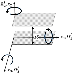
Figure 2: Flow configuration and coordinate system.

5.1 Heated Couette flows

Initially, we evaluate the model performance in a fully-developed Couette flow with the top wall moving at constant speed $u_{w}$ relative to the bottom wall. As a result, the mean flow is driven by the shear stress due to the relative movement between top and bottom walls, while the temperature difference between the heated top wall and the cooled bottom wall is kept constant. We consider two cases at different Reynolds numbers, particularly $Re_{w}=\frac{2\,u_{w}\,\delta}{\nu}=8600$ and 12800, for which detailed DNS data are provided by Kawamura et al. [24]. Figures LABEL:fig:COUETTE_ScF_8600 and LABEL:fig:COUETTE_ScF_12800 show a comparison between the two models (proposed and Younis) for the scalar-flux components with the corresponding DNS results for the two cases. Regarding the streamwise component, both models perform well near the wall boundary, being able to capture both the magnitude and the location of the near-wall peak, while both closures predict faster reduction of the shape profile with respect to the DNS results while moving away from the wall. The proposed model agrees well with the DNS data for the wall-normal component, especially at the wall region and close to the channel center, while Younis’ model underestimates the wall-normal component outside the viscous sublayer ($y^{+}>10$).

5.2 Heated Poiseuille flows

Here, we consider the case of a heated channel flow under fully-developed conditions at two different Reynolds numbers, particularly $Re_{\tau}=395$ and 640. The non-slip boundary condition is adopted in the wall-normal direction (i.e. at the top and bottom walls) while the thermal boundary condition is uniform heat-flux on both walls. The quality of the predictions is compared with the corresponding DNS results [17, 25]. Figure LABEL:fig:POISEUILLE_ScF_395_640 compares the turbulent scalar-fluxes as obtained from the present model and the Younis model for both cases. We observe that both models provide similar predictions for the streamwise component, achieving good agreement with the DNS data in both the inner and outer region of the channel. For the high $Re$ case though, both models tend to overpredict the magnitude of the peak value, thus showing a mild Reynolds dependence. Looking into the balance between the terms appearing in equation (18a) (not shown here) revealed that this tendency is mainly attributed to the $C_{3}$-related term, since this term exhibits the highest sensitivity to the Reynolds number. Contrary to algebraic closures, DNS predict non-zero values for the streamwise component at the channel centerline. This happens because the turbulent scalar field is being transported by the mean flow or the turbulence. These transport processes constitute a non-local mechanism that cannot be captured by a rational algebraic closure [9]. For the low $Re$ case, the proposed model achieves a considerably better agreement than Younis’ model regarding the normal flux, being able to quickly adjust to the slope’s sign change that occurs in the inner region. As expected, both models tend to overestimate the magnitude of the flux for $Re_{\tau}=640$, with the proposed model still being able to produce satisfactory results.

Next, we further investigate the near-wall performance of the proposed closure. A useful parameter for that purpose is the scalar-flux ratio $R_{u^{\prime}\phi^{\prime}}$, defined in equation (11). Figure LABEL:fig:POISEUILLE_ScR shows a comparison of the scalar-flux ratio predictions of both models (proposed and Younis) with the corresponding DNS data, for which this ratio varies as $R_{12}/R_{11}$ in the near-wall region under high shear strain, as already mentioned in Section 3. The proposed model achieves better agreement with the DNS results, being able to capture the near-wall limit up to $y^{+}=20$. This is attributed to the dominant role that $C_{5}$-related term plays in the buffer layer for both flux-components, as already shown in figure LABEL:fig:CALIBRATION_CASE, which exhibits the proper near-wall physical behaviour (see discussion in Section 3). In contrast, Younis’ model fails to capture this limiting behaviour for $y^{+}>10$, since no term appearing in its model equation (6) captures the correct turbulent anisotropy.

5.3 Heated channel flow subjected to streamwise rotation

The first considered case involving Coriolis effects is that of a flow in a plane channel that rotates about its streamwise axis. This scenario is more complex than the stationary one, since it induces a non-trivial spanwise mean velocity component, thus activating additional Reynolds stress elements. The walls are assumed to be kept at different, but constant temperatures without fluctuations, with the upper wall cooled and the lower wall heated. Comparison is made with DNS studies that differ substantially in the relative strength of the imposed rotation. The first study corresponds to the DNS results of Wu & Kasagi [26] for Rossby and Reynolds numbers $Ro_{\tau}=\frac{2\Omega^{f}_{1}\delta}{u^{*}_{\tau}}=2.5$ and $Re_{\tau^{*}}=\frac{u^{*}_{\tau}\delta}{\nu}=300$ respectively, where $u^{*}_{\tau}$ is the friction velocity calculated from the wall shear stress averaged on the two walls. Figure LABEL:fig:RE_300_Ro25_ST shows results for the scalar-flux components. For the streamwise component, both models accurately capture the location and magnitude of the peak value. However, similar to the stationary cases, their predictions drop much faster than the DNS results while approaching the channel’s centerline. The present closure provides reasonable estimations for the normal component, being able to capture the near-wall anisotropy, while it mildly underestimates the level of this quantity while moving away from the wall. This happens possibly due to the fact that the effects of streamwise rotation on the normal component are explicitly absent, as indicated in equation (18b). The opposite is true for Younis’ formulation, for which this dependence enters via the $C_{4}$-related term, as implied by equation (6).

The second case study considered is by El-Samni & Kasagi [27] for $Re_{\tau^{*}}=163$ in the presence of a much stronger rotation rate, corresponding to $Ro_{\tau}=15$, whereas the thermal boundary conditions are the same as in the low-$Ro_{\tau}$ case. Figure LABEL:fig:RE_163_Ro15_ST shows profiles of the scalar-flux components, showing large discrepancies between DNS and models. Both models significantly overpredict the maximum value of the streamwise component. Regarding the proposed closure, this is partly associated with the presence of non-trivial contribution from the product $R_{12}\,R_{23}$ that appears in the $C_{5}$-related term of the model equation (18a). As a result, the value of this term is greatly increased compared to the stationary case. Significant increase (compared to the non-rotating case) also occurs for $C_{3}$-related term, suggesting that modifications to the associated model coefficient might be required so that the model attains the proper anisotropy levels. In accordance with the previous case study, the proposed model predicts smaller values for the normal component than Younis’ formulation, achieving better agreement with the DNS in the near wall region as well as close to channel’s centerline.

5.4 Heated channel flow subjected to wall-normal rotation

Here, the simulated flow field is rotated at a specified angular velocity around the wall-normal axis, which induces a strong spanwise mean velocity that makes the absolute mean flow tilt towards to the spanwise direction. The DNS results used for this case are those of El-Samni & Kasagi [27] at $Re_{\tau^{*}}=160.1$ and $Ro_{\tau}=0.04$. The profiles of the streamwise scalar-flux component are shown in figure LABEL:fig:RE_160_Ro004_WN_a. The models provide similar predictions, being able to capture accurately the near-wall peak while underestimating the value of this quantity in the remaining region. As shown in figure LABEL:fig:RE_160_Ro004_WN_b, Younis’ model achieves very accurate predictions for the normal component, while the present model underestimates the level of this quantity outside the proximity of the wall boundary ($y^{+}>20$).

5.5 Heated channel flow subjected to spanwise rotation

Next, we consider the presence of Coriolis forces emerging from the spanwise rotation. For this configuration, existing studies [28, 29] have shown that at moderate $Ro$ numbers, turbulence and especially the wall-normal fluctuations are augmented on the channel side where the system rotation is anti-cyclonic (called the unstable side), while they are damped on the channel side where the rotation is cyclonic (called the stable side). The scalar is kept at constant but different values at each wall, in accordance with the previous rotating cases. Model predictions are compared with the DNS results of Wu & Kasagi [26] for $Re_{\tau^{*}}=295.5$ and $Ro_{\tau}=2.5$. Figure LABEL:fig:RE_295_Ro25_SP_a shows that both models severely overestimate the level of the peak magnitude in the near-wall region. Focusing on the present model, the strength of the individual terms that contribute to this quantity (18a) is shown in figure LABEL:fig:RE_295_Ro25_SP_b. We observe the failure of the model in the near-wall region mainly because the $C_{3}$-related term becomes extremely high in the high-strain rate region, while it becomes trivial for $y^{+}>50$, yielding reasonable predictions of the model outside the buffer layer ($y^{+}>30$). Consequently, modifications on the damping function $f_{C_{3}}$ should be applied to improve model performance in this region. Figure 11 reveals that both models are sensitized to the rotation-induced asymmetry, with the proposed model being in closer agreement with the DNS results than Younis’ model. Note that equation (18b) indicates that the $C_{3}$-related term does not contribute to the estimation, thus supporting the notion that modifications on the $f_{C_{3}}$ can improve model performance for this case.

Figure 11: As in Figure LABEL:fig:RE_295_Ro25_SP_a, but for the wall-normal component.

6 SUMMMARY AND CONCLUSIONS

In this study we have proposed an explicit algebraic closure for the turbulent scalar-flux vector based on the general formulation of Younis, which is essentially an extended version of the model proposed by Abe & Suga (12) through the inclusion of an extra term involving products between the gradients of the mean velocity and scalar field. This closure consists of three terms, making it simpler than Younis’ model and an elegant choice for use in general-purpose computational codes. It is also motivated by the “effective-gradients” hypothesis, which postulates that turbulence-turbulence interactions provide a gradient that acts supplementary to the mean shear, thus giving an alternative physical interpretation of the proposal compared to other closures. The resulting model explicitly depends on Coriolis effects in a similar manner to other models, which ensures its consistency with the principle of coordinate invariance. To minimize model bias to inhomogeneous applications, the values of the model coefficients are determined based on existing LES predictions of homogeneous shear flows in the presence of arbitrary mean scalar gradients, while a simple damping function was applied to account for the near-wall effects. In order to test the quality of the proposed model, we have considered different types of heated channel flows, particularly Poiseuille and Couette flows, in both stationary and rotating frames. The proposed model performs well in Couette flows at different Reynolds numbers, showing its sensitivity to the near-wall turbulent anisotropies. Regarding Poiseuille flows, good predictions are obtained for both flux components, with the model showing a mild tendency to overestimate the near-wall peak magnitude as the Reynolds number increases. Furthermore, the proposed model captured the proper near-wall limit for the scalar ratio $R_{u^{\prime}\phi^{\prime}}$ for wall distances up to $y^{+}\approx 20$, significantly further than Younis’ model ($y^{+}\approx 10$). In all cases, the proposed model achieved substantially better agreement with the DNS results than Younis’ model for the normal component, while similar predictions between the models have been obtained for the streamwise component. The above non-rotating cases served as a guidance regarding the role of the different terms appearing in the algebraic expressions, showing the ability of the proposal to capture the anisotropy between the different flux components. The performance of the proposed model was further challenged in heated channel flows subjected to different modes of rotation, resulting in more complex flow configurations due to the emergence of secondary flows. Generally, the presented algebraic expression provides reasonable predictions for the normal component. Under spanwise rotation though, the model fails in capturing the proper near-wall behavior (the same is also evident with Younis model) of the streamwise component, suggesting that further modifications on the damping functions should be investigated. Future work will focus on testing the proposed closure in additional cases involving frame-rotation, in an attempt to further improve the estimation performance in the presence of Coriolis effects. For that purpose, we intend to use DNS data in heated channel flows to quantify the response of passive scalar transport for a wider range of Rossby numbers.

Appendix A Details regarding the calibration process.

The model coefficients of the proposed algebraic closures are determined based on the LES data of Kaltenbach et al. [15], who investigated the turbulent transport of three passive species which have uniform gradients in either the normal, streamwise or spanwise direction. All cases under consideration start from the same shear parameter ratio $S^{*}_{o}=\bigg{(}\frac{2S\kappa}{\epsilon}\bigg{)}_{o}=5.04$ and the same Prandtl number $Pr=1.0$, in the initial absent of scalar fluctuations. The mean flow configuration is expressed by

$$G_{ij}=S\delta_{i1}\delta_{j3}\,,\qquad\Lambda_{i}=\Lambda\delta_{i\alpha}\,,$$ (19)

where greek index $\alpha$ denotes the direction of the mean scalar gradient.

$St$	$R_{11}$	$R_{13}$	$R_{22}$	$R_{33}$	$\epsilon$	$\Lambda_{i}$	$\overline{u^{\prime}_{1}\phi^{\prime}}$	$\overline{u^{\prime}_{2}\phi^{\prime}}$	$\overline{u^{\prime}_{3}\phi^{\prime}}$
8	4.98	-1.42	2.82	1.60	0.911	$(1,0,0)$	-10.9		2.22
10	6.32	-1.84	3.63	2.20	1.190	$(1,0,0)$	-13.9		3.01
12	7.67	-2.27	4.71	3.12	1.600	$(1,0,0)$	-16.3		4.08
8	4.98	-1.42	2.82	1.60	0.911	$(0,1,0)$		-3.84
10	6.32	-1.84	3.63	2.20	1.190	$(0,1,0)$		-4.62
12	7.67	-2.27	4.71	3.12	1.600	$(0,1,0)$		-5.78
8	4.98	-1.42	2.82	1.60	0.911	$(0,0,1)$	4.32		-1.83
10	6.32	-1.84	3.63	2.20	1.190	$(0,0,1)$	5.42		-2.47
12	7.67	-2.27	4.71	3.12	1.600	$(0,0,1)$	6.33		-3.42

Table 1: Summary of the LES data used to determine model coefficients. Data are extracted at different total shear instants $St$ (where $t$ is time).

References

- [1] B.A. Younis, B. Weigand, F. Mohr, and M. Schmidt. Modeling the effects of system rotation on the turbulent scalar fluxes. J. Heat Transf., 132(5):051703, 2010. doi: 10.1115/1.4000446.
- [2] G.K. Batchelor. Diffusion in a field of homogeneous turbulence. Aust. J. Sci. Res. Ser. A, 2:437–450, 1949. doi: 10.1071/PH490437.
- [3] B.J. Daly and F.H. Harlow. Transport equations of turbulence. Phys. Fluids, 13 (11):2634–2649, 1970. doi: 10.1063/1.1692845.
- [4] K. Suga and K. Abe. Nonlinear eddy viscosity modelling for turbulence and heat transfer near wall and shear-free boundaries. Int. J. Heat Fluid Fl., 21(1):37–48, 2000. doi: 10.1016/S0142-727X(99)00060-0.
- [5] W. Rodi. The prediction of free turbulent boundary layers by use of a two-equation model of turbulence. PhD Thesis, Department of Heat Transfer, Imperial College, London, 1972.
- [6] S.S. Girimaji and S. Balachandar. Analysis and modeling of buoyancy-generated turbulence using numerical data. Int. J. Heat Mass Tran., 41 (6-7):915–929, 1998. doi: 10.1016/S0017-9310(97)00166-X.
- [7] P.M. Wikstrom, S. Wallin, and A.V. Johansson. Derivation and investigation of a new explicit algebraic model for the passive scalar flux. Phys. Fluids, 12:688–702, 2000. doi: 10.1063/1.870274.
- [8] W.M.J. Lazeroms, G. Brethouwer, S. Wallin, and A.V. Johansson. An explicit algebraic Reynolds-stress and scalar-flux model for stably stratified flows. J. Fluid Mech., 723:91–125, 2013. doi: 10.1017/jfm.2013.116.
- [9] B.A. Younis, C.G. Speziale, and T.T. Clark. A rational model for the turbulent scalar fluxes. Proc. R. Soc. A, 461:575–594, 2005. doi: 10.1098/rspa.2004.1380.
- [10] B.A. Younis, B. Weigand, and S. Spring. An explicit algebraic model for turbulent heat transfer in wall-bounded flow with streamline curvature. J. Heat Transf., 129(4):425–433, 2007. doi: 10.1115/1.2709960.
- [11] H. Müller, B.A. Younis, and Weigand B. Development of a compact explicit algebraic model for the turbulent heat fluxes and its application in heated rotating flows. Int. J. Heat Mass Tran., 86:880–889, 2015. doi: 10.1016/j.ijheatmasstransfer.2015.03.059.
- [12] B.E. Launder, D.P. Tselepidakis, and B.A. Younis. A second-moment closure study of rotating channel flow. J. Fluid Mech., 183:63–75, 1987. doi: 10.1017/S0022112087002520.
- [13] T. Dakos and M.M. Gibson. On modelling the pressure terms of the scalar flux equations. pages 7–18. Turbulent Shear Flows 5. Springer, Berlin, Heidelberg, 1987. doi: 10.1007/978-3-642-71435-1_2.
- [14] A. Yoshizawa. Statistical analysis of the anisotropy of scalar diffusion in turbulent shear flows. Phys. Fluids, 28(11):3226–3231, 1985. doi: 10.1063/1.865371.
- [15] H.J. Kaltenbach, T. Gerz, and U. Schumann. Large-eddy simulation of homogeneous turbulence and diffusion in stably stratified shear flow. J. Fluid Mech., 280:1–40, 1994. doi: 10.1017/S0022112094002831.
- [16] B.E. Launder. On the computation of convective heat transfer in complex turbulent flows. J. Heat Transf., 110(4b):1112–1128, 1988. doi: 10.1115/1.3250614.
- [17] K. Abe and K. Suga. Towards the development of a Reynolds-averaged algebraic turbulent scalar-flux model. Int. J. Heat Fluid Fl., 22(1):19–29, 2001. doi: 10.1016/S0142-727X(00)00062-X.
- [18] J. Kim and P. Moin. Transport of passive scalars in a turbulent channel flow. In Andre JC., J. Cousteix, F. Durst, B.E. Launder, F.W. Schmidt, and J.H. Whitelaw, editors, Turbulent Shear Flows, volume 6. Springer, Berlin, Heidelberg, 1989.
- [19] Y. Tomita, N. Kasagi, and A. Kuroda. Establishment of the Direct Numerical Simulation databases of turbulent transport phenomena. http://thtlab.jp/DNS/CH122_PG.WL1, 1993.
- [20] S.C. Kassinos and W.C. Reynolds. A structure-based model with stropholysis effects. Annual Research Briefs, pages 197–209, California, USA, 1998. Center for Turbulence Research, NASA Ames/Stanford University.
- [21] C.F. Panagiotou and S.C. Kassinos. A structure-based model for the transport of passive scalars in homogeneous turbulent flows. Int. J. Heat Fluid Fl., 57:109–129, 2016. doi: 10.1016/j.ijheatfluidflow.2015.11.008.
- [22] C.F. Panagiotou and S.C. Kassinos. A structure-based model for transport in stably stratified homogeneous turbulent flows. Int. J. Heat Fluid Fl., 65:309–322, 2017. doi: 10.1016/j.ijheatfluidflow.2016.12.005.
- [23] C.F. Panagiotou, F.S. Stylianou, and S.C. Kassinos. Structure-based transient models for scalar dissipation rate in homogeneous turbulence. Int. J. Heat Fluid Fl., XX:XX, 2020.
- [24] H. Kawamura, H. Abe, and K. Shingai. DNS of turbulence and heat transport in a channel flow with different Reynolds and Prandtl numbers and boundary conditions. In Y. Nagano, K. Hanjalic, and T. Tsuji, editors, 3rd International Symposium on Turbulence, Heat and Mass Transfer, volume 6. Aichi Shuppan, 2000.
- [25] H. Abe, H. Kawamura, and Y. Matsuo. Surface heat-flux fluctuations in a turbulent channel flow up to =1020 with Pr=0.025 and 0.71. Int. J. Heat Fluid Fl., 25(3):404–419, 2004. doi: 101016/jijheatfluidflow200402010.
- [26] H. Wu and N. Kasagi. Effects of arbitrary directional system rotation on turbulent channel flow. Phys. Fluids, 16(4):979–990, 2004. doi: 10.1063/1.1649337.
- [27] O. El-Samni and N. Kasagi. Heat and momentum transfer in rotating turbulent channel flow. In 4th JSME-KSME Thermal Engi. Conf., volume 3. Kobe, 2000.
- [28] O. Grundestam, S. Wallin, and A.V Johansson. Direct numerical simulations of rotating turbulent channel flow. J. Fluid Mech., 598:177–199, 2008. doi: 10.1017/S0022112007000122.
- [29] Z. Xia, Y. Shi, and S. Chen. Direct numerical simulation of turbulent channel flow with spanwise rotation. J. Fluid Mech., 788:42–56, 2016. doi: 10.1017/jfm.2015.717.