Verification benchmarks for single-phase flow in three-dimensional fractured porous media

Abstract

Flow in fractured porous media occurs in the earth’s subsurface, in biological tissues, and in man-made materials. Fractures have a dominating influence on flow processes, and the last decade has seen an extensive development of models and numerical methods that explicitly account for their presence. To support these developments, we present a portfolio of four benchmark cases for single-phase flow in three-dimensional fractured porous media. The cases are specifically designed to test the methods’ capabilities in handling various complexities common to the geometrical structures of fracture networks. Based on an open call for participation, results obtained with 17 numerical methods were collected. This paper presents the underlying mathematical model, an overview of the features of the participating numerical methods, and their performance in solving the benchmark cases.

1 Introduction

Flow in fractured porous media is characterized by an interaction between the fractures and the surrounding porous medium, commonly referred to as the matrix. The strong influence of fracture network geometry on flow patterns has motivated the development of mathematical models and numerical methods that explicitly account for the geometry of fractures [1]. Considering flow both in the fractures and in the surrounding porous medium, these models are based on the conceptual discrete-fracture-matrix (DFM) representation of the fractured porous media.

With the development of a wealth of simulation tools for flow in fractured porous media, a need for verification benchmarks for numerical methods has emerged. To accommodate this need, four research groups working in the field initiated a comparison study, which led to the presentation of a suite of two-dimensional benchmark tests and corresponding results for a range of numerical methods [2]. The methods were probed on test cases featuring known difficulties for numerical methods, including fracture intersections and combinations of blocking and conducting fractures. The study exposed the relative strengths and weaknesses between the participating methods, both in terms of accuracy and computational cost. After the publication of the results, these benchmark cases have been widely applied by the scientific community in testing numerical methods and new simulation tools [3, 4, 5, 6, 7, 8, 9, 10, 11].

Based on the reception of the verification benchmarks [2] and the capabilities of three-dimensional modeling in the research community, the next phase in the work on verification benchmarks was launched with a call for participation [12]. The purpose of this call was to extend the platform of verification benchmarks for numerical methods to three-dimensional problems. In addition, the studies were extended to include simulations of linear tracer transport as a means to highlight additional nuances in the comparison of the calculated flow fields. The present paper discusses the results we received as answers to this call.

The paper is organized as follows. In Section 2, an overview of the participation process is given. In Section 3, we describe the mathematical models for fluid flow and transport in fractured porous media. Section 4 briefly describes the participating numerical methods as well as the discretization of the transport problem. The four test cases are described in Section 5, with each description followed by a presentation and discussion of the corresponding results. Section 6 summarizes the discussion of the results, and Section 7 provides concluding remarks.

2 Benchmark Process

The publication of this verification benchmark study was laid out as a four-stage process: the development of benchmark cases, a call for participation, collection and synchronization of the results by the participants, and a final discussion and reporting.

The process started with the participants of the benchmark study [2] developing four new test cases. These were designed to test the capabilities of numerical methods for DFM representations of flow in three-dimensional fracture networks. The design of each test case was led by the ”benchmark case designers” listed in Section 5. An open call for participation was launched in September 2018 [12], followed by a dedicated mini-symposium at the SIAM Conference on Mathematical and Computational Issues in the Geosciences, March 2019, Houston. Researchers interested in participating in the benchmark followed a predefined registration procedure, were approved by the authors issuing the call, and were asked to sign a participation agreement. During this process, we received applications concerning 15 additional numerical methods, all of which were approved. Finally, the results of 12 of these methods were submitted and included in the study.

The case descriptions presented in the call [12] were accompanied by data in the form of geometry descriptions, existing simulation results, and plotting scripts, all available in the Git repository https://git.iws.uni-stuttgart.de/benchmarks/fracture-flow-3d.git. This repository was reused in the fully transparent collection and synchronization phase. During this phase, the results were uploaded and made available to all participants, and recomputations and adjustments were allowed until August 2019. In the fourth phase, all participants contributed to the reporting of the results presented in Section 5. The last two phases were led by assigned ”benchmark case coordinators”. While access to the Git repository was restricted to the benchmark participants during the phase of collection and comparison of the results, all data have been made publicly available upon submission of this manuscript. In addition to the data and plotting scripts, five Jupyter notebooks are provided, four focusing on reproducing the figures encountered in Section 5, and one for facilitating the comparison of new results.

3 Mathematical Models

We introduce two models for flow and transport in fractured media. First, the flow model is presented in the conventional equidimensional setting, allowing a natural introduction to the physical parameters. From this formulation, we derive the mixed-dimensional model through appropriate reduction of the equations. The mixed-dimensional model forms the focus of this study. Finally, we present the equi- and mixed-dimensional transport models.

3.1 Equidimensional Flow Model

We consider a steady-state, incompressible, single-phase flow through a porous medium described by Darcy’s law. With the imposition of mass conservation, the governing system of equations is given by

$$\begin{aligned} \bm{u}+\mathbb{K}\nabla h&=0,\\ \nabla\cdot\bm{u}&={q},\end{aligned}\quad\text{in }\Lambda.$$ (1a)

Here, $$\bm{u} \mathrm{m}\text{/}\mathrm{s} \mathbb{K} \mathrm{m}\text{/}\mathrm{s} h \mathrm{m}\text{/} q \text{/}\mathrm{s} \Lambda\subset\mathbb{R}^{3} \partial\Lambda \Lambda$$ denotes the fluid velocity in , is hydraulic conductivity measured in , is hydraulic head measured in , and represents a source/sink term measured in . The domain will be called the equidimensional domain. The following boundary conditions on the boundary of complete model (1a):

$$\begin{aligned} h|_{{\partial\Lambda_{{\footnotesize h}}}}&=\overline{h}&\quad\text{on }{\partial\Lambda_{{\footnotesize h}}},\\ \bm{u}\cdot\bm{n}|_{{\partial\Lambda_{{\footnotesize u}}}}&=\overline{u}&\text{on }{\partial\Lambda_{{\footnotesize u}}}.\end{aligned}$$ (1b)

We assume $\partial\Lambda={\partial\Lambda_{{\footnotesize h}}}\cup{\partial\Lambda_{{\footnotesize u}}}$, ${\partial\Lambda_{{\footnotesize h}}}\cap{\partial\Lambda_{{\footnotesize u}}}=\emptyset$, and $|{\partial\Lambda_{{\footnotesize h}}}|>0$. In (1b) $\cdot|_{A}$ is a suitable trace operator on $A\subset\partial\Lambda$. $\overline{h}$ is the hydraulic head imposed on the boundary ${\partial\Lambda_{{\footnotesize h}}}$, while $\overline{u}$ is the prescribed Darcy velocity normal to the boundary ${\partial\Lambda_{{\footnotesize u}}}$ with respect to the outer unit normal vector $\bm{n}$.

By substituting Darcy’s law in the mass conservation, the dual problem (1) can be recast in its primal formulation, given by

$$\begin{aligned} -\nabla\cdot\mathbb{K}\nabla h&={q}&\quad\text{in }\Lambda,\\ h|_{{\partial\Lambda_{{\footnotesize h}}}}&=\overline{h}&\text{on }{\partial\Lambda_{{\footnotesize h}}},\\ -\mathbb{K}\nabla h\cdot\bm{n}|_{{\partial\Lambda_{{\footnotesize u}}}}&=\overline{u}&\text{on }{\partial\Lambda_{{\footnotesize u}}}.\end{aligned}$$ (2)

Problems (1) and (2) are equivalent. However, different numerical schemes are based on either of the two formulations. Under regularity assumptions on $\Lambda$ and the data, both problems admit a unique weak solution. We refer to [13, 14, 15, 16] for more details.

We assume that $\Lambda$ contains several fractures, i.e., thin inclusions in the domain. The fracture walls are assumed to be planar with smooth boundaries. The fractures have two distinguishing features: (1) the thickness, which we measure by the aperture $\varepsilon$, is small compared to the extension of the fracture; and the (2) hydraulic conductivity may differ significantly from that of the rest of $\Lambda$. The latter implies that the fractures may have a significant impact on the flow in $\Lambda$.

We further make the assumption that the principal directions of the local hydraulic conductivity are aligned with the orientation of the fractures. In particular, the hydraulic conductivity in the matrix ($\mathbb{K}_{3}$), the fractures ($\mathbb{K}_{2}$), as well as in the intersections between two fractures ($\mathbb{K}_{1}$) and at the crossings of intersections ($\mathbb{K}_{0}$), can be decomposed in the following way:

$$\mathbb{K}_{3} =K_{3}^{eq}, \mathbb{K}_{2} =\begin{bmatrix}K_{2}^{eq}&\begin{matrix}0\\ 0\end{matrix}\\ \begin{matrix}0&0\end{matrix}&\kappa_{2}^{eq}\end{bmatrix},$$

$$\mathbb{K}_{1} =\begin{bmatrix}K_{1}^{eq}&0&0\\ 0&\kappa_{1}^{eq}&0\\ 0&0&\kappa_{1}^{eq}\\ \end{bmatrix}, \mathbb{K}_{0} =\begin{bmatrix}\kappa_{0}^{eq}&0&0\\ 0&\kappa_{0}^{eq}&0\\ 0&0&\kappa_{0}^{eq}\\ \end{bmatrix}.$$

Here, $K_{d}^{eq}$ and $\kappa_{d}^{eq}$, for different values of $d$, denote the tangential and normal hydraulic conductivities, respectively. Thus, $K_{d}^{eq}$ is an elliptic $(d\times d)$-tensor field, whereas $\kappa_{d}^{eq}$ is a positive scalar field. The subscript $d$ indicates that the features will be represented by $d$-dimensional objects in the reduced model, as derived in the next section. The superscript $eq$, on the other hand, indicates that these quantities are related to the equidimensional model.

3.2 Mixed-dimensional Flow Model

The small aperture of the fractures justifies a reduction of dimensionality to a representation where fractures and their intersections are approximated by lower-dimensional objects. For more details on the derivation, we refer the reader to [17, 18, 19, 20, 21, 22, 23, 24, 25].

Here, we use $\Omega$ to denote the mixed-dimensional decomposition of $\Lambda$. First, let $\Omega$ contain a three-dimensional domain $\Omega_{3}$ that represents the (possibly unconnected) matrix. Furthermore, $\Omega$ contains up to three lower-dimensional, open subdomains, namely, the union of fracture planes $\Omega_{2}$, their intersection lines $\Omega_{1}$ and intersection points $\Omega_{0}$. For compatibility, we assume that $\Omega_{d}\not\subset\Omega_{d^{\prime}}$ for all $d^{\prime}>d$. Finally, we introduce $\Gamma_{d}=\Omega_{d}\cap\partial\Omega_{d+1}$ as the set of $d$-interfaces between neighboring subdomains of codimension one. Each interface is endowed with a normal unit vector $\bm{n}$ pointing outward from $\Omega_{d+1}$.

Remaining consistent with the notation convention above, data and unknowns will also be annotated with a subscript related to the dimension. As a first example, on a $d$-dimensional feature $\Omega_{d,i}\subseteq\Omega_{d}$ with counting index $i$, let $\varepsilon_{d,i}$ denote the cross-sectional volume, area, or length of the corresponding physical domain for $d=0,...,2$, respectively. It has the unit of measure ${\mathrm{m}}^{3-d}\text{/}$ and is extended as nondimensional unity in $\Omega_{3}$. Moreover, we introduce for each $d$-feature with index $i$, a typical length $a_{d,i}$ such that $\varepsilon_{d,i}=a_{d,i}^{3-d}$. In the continuation, we will omit the subscript $i$ if no ambiguity arises.

We continue this subsection by presenting the reduced model associated with (1) in the two-dimensional fractures $\Omega_{2}$ followed by its generalization for all $d=0,...,3$.

3.2.1 Two-dimensional Fracture Flow

The variables in this formulation are the velocity $\bm{u}_{3}=\bm{u}$ and hydraulic head $h_{3}=h$ in the rock matrix $\Omega_{3}$, as well as the integrated tangential velocity $\bm{u}_{2}$ and average hydraulic head $h_{2}$ in the fracture. These are given pointwise for $x\in\Omega_{2}$ by

$$\bm{u}_{2}(x)=\int_{\varepsilon_{2}(x)}\bm{u}_{\|}\quad\text{and}\quad h_{2}(x)=\dfrac{1}{\varepsilon_{2}(x)}\int_{\varepsilon_{2}(x)}h.$$

Here, $\bm{u}_{\|}$ denotes the components of $\bm{u}$ tangential to $\Omega_{2}$. The integrals are computed in the normal direction of the fracture, and thus, the corresponding units of measurement are ${\mathrm{m}}^{2}\text{/}\mathrm{s}$ and $\mathrm{m}\text{/}$ for $\bm{u}_{2}$ and $h_{2}$, respectively.

We derive the reduced Darcy’s law and the mass balance equation by averaging and integrating, respectively, over the direction normal to the fractures. Recall that the vector $\bm{n}$ here refers to the normal unit vector oriented outward from $\Omega_{3}$.

$$\begin{aligned} \frac{1}{\varepsilon_{2}}\bm{u}_{2}+K_{2}^{eq}\nabla_{2}h_{2}&=0\\ \nabla_{2}\cdot\bm{u}_{2}-\left\llbracket{\bm{u}_{3}\cdot\bm{n}}\right\rrbracket&={q}_{2}\end{aligned}\quad\text{in }\Omega_{2},$$ (3a)

where $$\nabla_{2} {q}_{2} {q}_{2}(s)=\int_{\varepsilon_{2}(s)}{q} K_{2}^{eq} \Omega_{2} \left\llbracket{\bm{u}_{3}\cdot\bm{n}}\right\rrbracket|_{\Omega_{d}}=\sum(\bm{u}_{3}\cdot\bm{n}|_{\Gamma_{2}}) \Omega_{2,i}\subseteq\Omega_{2} \Gamma_{2} \Omega_{2,i} \Omega_{2} \partial\Omega_{3}$$ is the del-operator in the tangential directions and is the integrated source term, i.e., . Note that we have assumed to be constant in the direction normal to . The jump operator is defined as , thus representing the mass exchange between fracture and matrix. In particular, for each subdomain , we sum over all flux contributions over sections of that coincide geometrically with . These fluxes are assumed to satisfy the following Darcy-type law given by a finite difference between the hydraulic head in and on :

$$\bm{u}_{3}\cdot\bm{n}+\kappa_{2}^{eq}\frac{2}{a_{d}}(h_{2}-h_{3})=0\quad\text{on }\Gamma_{2}.$$ (3b)

Note that to be mathematically precise, each term in this equation represents an appropriate trace or projection of the corresponding variable onto $\Gamma_{2}$.

3.2.2 Generalized Flow Model

Next, we generalize the equations described above to domains of all dimensions, thus including the intersection lines and points. For that purpose, we introduce the integrated velocity $\bm{u}_{d}$ for $d=1$ and average hydraulic head $h_{d}$ with $d=0,1$ given pointwise for $x\in\Omega_{d}$ by

$$\bm{u}_{1}(x)=\int_{\varepsilon_{1}(x)}\bm{u}_{\|}\quad\text{and}\quad h_{d}(x)=\dfrac{1}{\varepsilon_{d}(x)}\int_{\varepsilon_{d}(x)}h,\text{ for }d=0,1.$$

Again, $\bm{u}_{\|}$ denotes the components of $\bm{u}$ tangential to $\Omega_{1}$. The corresponding units of measurement are ${\mathrm{m}}^{3}\text{/}\mathrm{s}$ and $\mathrm{m}\text{/}$ for $\bm{u}_{1}$ and $h_{d}$, respectively. The analogs of (3a) on these lower-dimensional manifolds are then given by

$$\begin{aligned} \frac{1}{\varepsilon_{1}}\bm{u}_{1}+K_{1}^{eq}\nabla_{1}h_{1}&=0\\ \nabla_{1}\cdot\bm{u}_{1}-\left\llbracket{\bm{u}_{2}\cdot\bm{n}}\right\rrbracket&={q}_{1}\quad\text{in }\Omega_{1},\\ -\left\llbracket{\bm{u}_{1}\cdot\bm{n}}\right\rrbracket&={q}_{0}\quad\text{in }\Omega_{0}.\end{aligned}$$ (4)

Here, $\nabla_{1}$ denotes the del-operator, i.e., the derivative, in $\Omega_{1}$. Moreover, the linear jump operator $\left\llbracket{\cdot}\right\rrbracket$ is naturally generalized to $\left\llbracket{\bm{u}_{d+1}\cdot\bm{n}}\right\rrbracket|_{\Omega_{d}}=\sum(\bm{u}_{d+1}\cdot\bm{n}|_{\Gamma_{d}})$, where we for each subdomain $\Omega_{d,i}\subseteq\Omega_{d}$ sum over all flux contributions over sections of $\Gamma_{d}$ that coincide geometrically with $\Omega_{d,i}$. Finally, $q_{1}$ and $q_{0}$ correspond to the integrated source terms in the intersection lines and points, respectively.

Due to our choice of defining $\bm{u}_{d}$ as the integrated velocity, a scaling with $\varepsilon_{d+1}$ appears in the equation governing the flux across $\Gamma_{d}$:

$$\frac{1}{\epsilon_{d+1}}\bm{u}_{d+1}\cdot\bm{n}+\kappa_{d}^{eq}\frac{2}{a_{d}}(h_{d}-h_{d+1})=0\quad\text{on }\Gamma_{d},\ d=0,1.$$ (5)

Recalling that $\epsilon_{3}=1$, it now follows that the effective tangential and normal hydraulic conductivities are given by:

$$K_{d} =\varepsilon_{d}K_{d}^{eq}, \text{in }\Omega_{d},\ d =1,\dots,3$$ (6a)

$$\kappa_{d} =\varepsilon_{d+1}\frac{2}{a_{d}}\kappa_{d}^{eq}, \text{on }\Gamma_{d},\ d =0,\dots,2.$$ (6b)

From these definitions, it is clear that the units of $K_{d}$ and $\kappa_{d}$ are ${\mathrm{m}}^{4-d}\text{/}\mathrm{s}$ and ${\mathrm{m}}^{2-d}\text{/}\mathrm{s}$, respectively.

Collecting the above equations, we obtain the generalization of system (3) to subdomains of all dimensions. The resulting system consists of Darcy’s law in both tangential and normal directions followed by the mass conservation equations:

$$\bm{u}_{d}+K_{d}\nabla_{d}h_{d} =0, \Omega_{d},\ d=1,\dots,3,$$ in (7a)

$$\bm{u}_{d+1}\cdot\bm{n}+\kappa_{d}(h_{d}-h_{d+1}) =0, \Gamma_{d},\ d=0,\dots,2,$$ on (7b)

$$\nabla_{d}\cdot\bm{u}_{3} ={q}_{3}, \Omega_{3},$$ in (7c)

$$\nabla_{d}\cdot\bm{u}_{d}-\left\llbracket{\bm{u}_{d+1}\cdot\bm{n}}\right\rrbracket ={q}_{d}, \Omega_{d},\ d=1,2,$$ in (7d)

$$-\left\llbracket{\bm{u}_{1}\cdot\bm{n}}\right\rrbracket ={q}_{0}, \Omega_{0}.$$ in (7e)

The source term is given by ${q}_{3}$ for the rock matrix and ${q}_{d}(x)=\int_{\varepsilon_{d}(x)}{q}$ measured in ${\mathrm{m}}^{3-d}\text{/}\mathrm{s}$.

System (7) is then compactly described by:

$$\bm{u}_{d}+K_{d}\nabla_{d}h_{d} =0, \text{in }\Omega_{d},\ d =1,\dots,3,$$ (8a)

$$\bm{u}_{d+1}\cdot\bm{n}+\kappa_{d}(h_{d}-h_{d+1}) =0, \text{on }\Gamma_{d},\ d =0,\dots,2,$$ (8b)

$$\nabla_{d}\cdot\bm{u}_{d}-\left\llbracket{\bm{u}_{d+1}\cdot\bm{n}}\right\rrbracket ={q}_{d}, \text{in }\Omega_{d},\ d =0,\dots,3,$$ (8c)

in which the nonphysical $\bm{u}_{4}$ and $\bm{u}_{0}$ are understood as zero. The boundary conditions are inherited from the equidimensional model with the addition of a no-flux condition at embedded fracture endings:

$$h_{d} =\overline{h} \text{on }\partial\Omega_{d}\cap{\partial\Lambda_{{\footnotesize h}}},\ d =0,\dots,3,$$ (9a)

$$\bm{u}_{d}\cdot\bm{n} =\varepsilon_{d}\overline{u} \text{on }\partial\Omega_{d}\cap{\partial\Lambda_{{\footnotesize u}}},\ d =1,\dots,3,$$ (9b)

$$\bm{u}_{d}\cdot\bm{n} =0 \text{on }\partial\Omega_{d}\backslash(\Gamma_{d-1}\cup\partial\Lambda),\ d =1,\dots,3.$$ (9c)

To finish the section, we present the primal formulation of the mixed-dimensional fracture flow model. Analogous to (2), this formulation is derived by substituting Darcy’s laws (8a) and (8b) into the conservation equation (8c):

$$-\nabla_{d}\cdot K_{d}\nabla_{d}h_{d}+\left\llbracket{\kappa_{d}(h_{d}-h_{d+1})}\right\rrbracket ={q}_{d}, \text{in }\Omega_{d},\ d =0,\dots,3.$$ (10)

Again, we interpret the divergence term as zero if $d=0$ and the jump term as zero if $d=3$. The boundary conditions are given by

$$h_{d} =\overline{h} \text{on }\partial\Omega_{d}\cap{\partial\Lambda_{{\footnotesize h}}},\ d =0,\dots,3,$$ (11a)

$$-K_{d}\nabla_{d}h_{d}\cdot\bm{n} =\varepsilon_{d}\overline{u} \text{on }\partial\Omega_{d}\cap{\partial\Lambda_{{\footnotesize u}}},\ d =1,\dots,3,$$ (11b)

$$-K_{d}\nabla_{d}h_{d}\cdot\bm{n} =0 \text{on }\partial\Omega_{d}\backslash(\Gamma_{d-1}\cup\partial\Lambda),\ d =1,\dots,3.$$ (11c)

Many discretization schemes presented in this study ignore flow in the one-dimensional fracture intersections and zero-dimensional intersections thereof. Although these correspond to discretizing a simpler model, this is perfectly in line with the proposed study.

3.3 Equidimensional Transport Model

We now consider a scalar quantity $c$ with the unit of measure ${\mathrm{m}}^{-3}\text{/}$, which is transported through the porous medium subject to the velocity field resulting from the flow model presented in the previous sections. The purely advective transport of $c$ is described by the conservation equation:

$$\phi\frac{\partial c}{\partial{t}}+\nabla\cdot\left(c\bm{u}\right)={q}_{c}\quad\text{in }\Lambda,$$ (12)

where $\phi$ is the porosity of the medium and ${q}_{c}$ is a source/sink term for $c$ given in ${\mathrm{m}}^{-3}\text{/}\mathrm{s}$. We define Dirichlet boundary conditions on those boundary segments where inflow occurs, i.e.,

$$c|_{\partial\Lambda_{\footnotesize c}}=\overline{c}\quad\text{on }\partial\Lambda_{\footnotesize c},\quad\partial\Lambda_{\footnotesize c}=\{x\in\partial\Lambda:\,\,\bm{u}\cdot\bm{n}<0\},$$ (13)

with $\overline{c}$ being the value for $c$ prescribed on the boundary $\partial\Lambda_{\footnotesize c}$.

3.4 Mixed-dimensional Transport Model

Analogous to Section 3.2, we choose the average value for $c$ as the primary variable, which is defined as $c_{3}=c$ in $\Omega_{3}$ and for the lower dimensional objects (with $d\leq 2$) as

$$c_{d}(s)=\dfrac{1}{\varepsilon_{d}(s)}\int_{\varepsilon_{d}(s)}c.$$

Following the derivation of the mixed-dimensional flow model presented in Section 3.2, the resulting mixed-dimensional transport model reads as:

$$\varepsilon_{d}\phi_{d}\frac{\partial c_{d}}{\partial{t}}+\nabla_{d}\cdot\left(c_{d}\bm{u}_{d}\right)-\left\llbracket{\tilde{c}_{d+1}\left(\bm{u}_{d+1}\cdot\bm{n}\right)}\right\rrbracket={q}_{c,d}\quad\text{in }\Omega_{d},\quad d=0,\dots,3.$$ (14)

Note that for $d=0$, the divergence term is void. Here, the porosity is simply $\phi_{d}=\phi^{eq}$, with units of measure ${\mathrm{m}}^{-3}\text{/}$, and $\tilde{c}_{d+1}$ is evaluated on the basis of a first-order upwind scheme, i.e.,

$$\tilde{c}_{d+1}=\begin{cases}c_{d+1}&\text{if}\quad\bm{u}_{d+1}\cdot\bm{n}|_{\Gamma_{d}}>0\\ c_{d}&\text{if}\quad\bm{u}_{d+1}\cdot\bm{n}|_{\Gamma_{d}}<0.\end{cases}$$ (15)

As in the flow model, the jump operator represents the sum of the fluxes over all contributions defined on sections of $\Gamma_{d}$ that coincide geometrically with $\Omega_{d,i}$.

4 Discretization Methods

The intent of this benchmark study is to quantitatively evaluate different discretization schemes for the mixed-dimensional flow models (8)-(11). As a means of evaluation, the velocities were inserted into a standard cell-centered, first-order upwind scheme for the transport equations (14). The temporal discretization is given by the implicit Euler method with a fixed time-step prescribed for each test case. The main properties of the discretization methods covered by the benchmark are summarized in Tables 1 and 2, which also contain references for further details. The majority of the methods followed the mixed-dimensional flow model and the specified transport discretization, with the following exceptions:

The schemes NCU_TW-Hybrid_FEM and DTU-FEM_COMSOL describe the flow along the fractures by additional terms defined on the fracture surfaces. This effectively adds connectivity between the degrees of freedom located on fractures without introducing additional degrees of freedom. This means that these schemes do not solve the mass balances (8c) for $d<3$. Moreover, this approach implies continuity of the hydraulic head across the fractures and therefore replaces the coupling condition (8b). Other schemes participating in this study also assume continuity of the hydraulic head across the fractures, and a complete overview is given in Table 2.

The scheme UNIL_USI-FE_AMR_AFC is an equidimensional approach, meaning that the fractures, their intersections, and intersections of intersections are discretized with three-dimensional elements using locally refined grids. Therefore, the lower-dimensional mass balances (8c) for $d<3$ and the coupling conditions (8b) are not relevant for this scheme.

Finally, the schemes ETHZ_USI-FEM_LM and UNIL_USI-FE_AMR_AFC do not use a first-order upwind scheme but apply an algebraic flux correction technique for the stabilization of a finite element discretization of the transport model [26]. Such stabilization techniques provide a similar discretization as the given upwind scheme.

Acronym	References	Open source code	Run scripts	Test cases
Two-point flux approximation
UiB-TPFA	[27, 28]	✓[29]	[30]	1-4
Multi-point flux approximation
UiB-MPFA	[27, 28]	✓[29]	[30]	1-4
Lowest order mixed virtual element method
UiB-MVEM	[27, 28]	✓[29]	[30]	1-4
Lowest order Raviart-Thomas mixed finite elements
UiB-RT0	[27, 28, 25]	✓[29]	[30]	1-4
Multi-point flux approximation
USTUTT-MPFA	[31]	✓[32]	[33]	1-4
Two-point flux approximation
USTUTT-TPFA_Circ	[31]	✓[32]	[33]	1-4
Mimetic Finite Differences
LANL-MFD	[34]	✓[35]		1-4
Hybrid finite element method
NCU_TW-Hybrid_FEM	[36, 37]			1
Vertex Approximate Gradient continuous hydraulic head
UNICE_UNIGE-VAG_Cont	[38]			1-4
Hybrid Finite Volumes continuous hydraulic head
UNICE_UNIGE-HFV_Cont	[38]			1-4
Vertex Approximate Gradient discontinuous hydraulic head
UNICE_UNIGE-VAG_Disc	[39]			1-4
Hybrid Finite Volumes discontinuous hydraulic head
UNICE_UNIGE-HFV_Disc	[39]			1-4
Lagrange multiplier - L2-projection finite elements
ETHZ_USI-FEM_LM	[10, 40, 41]	✓	[42]	1-4
Hybrid H(div)
UNICAMP-Hybrid_Hdiv	[43, 44]	✓	[45]	1-4
Flux-corrected finite element method and adaptive mesh refinement
UNIL_USI-FE_AMR_AFC	[46, 26]			1-3
Embedded discrete fracture method
INM-EDFM	[47]	$\times$	$\times$	1,3
First-order Lagrangian finite elements (COMSOL)
DTU-FEM_COMSOL	[48]	$\times$	[49]	1-4

Table 1: Names, acronyms, references and test cases covered for all participating discretization methods.

Acronym	Degrees of freedom	Local mass conservation	Allows $h$ discontinuity	Conformity	subdomain dimensions
UiB-TPFA	$h$(elem), $\lambda$ (mortar flux)	✓	✓	geometrically	0-3
UiB-MPFA	$h$(elem), $\lambda$ (mortar flux)	✓	✓	geometrically	0-3
UiB-MVEM	$h$(elem), $\bm{u}$ (faces), $\lambda$ (mortar flux)	✓	✓	geometrically	0-3
UiB-RT0	$h$(elem), $\bm{u}$ (faces), $\lambda$ (mortar flux)	✓	✓	geometrically	0-3
USTUTT-MPFA	$h$(elem)	✓	✓	fully	2-3
USTUTT-TPFA_Circ	$h$(elem)	✓	✓	fully	2-3
LANL-MFD	$h$(faces)	✓	✓	fully	2-3
NCU_TW-Hybrid_FEM	$h$, $\bm{u}$(nodes)	✓	$\times$	fully	2-3
UNICE_UNIGE-VAG_Cont	$h$(nodes), (fracture faces)	✓	$\times$	conforming	2-3
UNICE_UNIGE-VAG_Disc	$h$(nodes), (fracture faces)	✓	✓	conforming	2-3
UNICE_UNIGE-HFV_Cont	$h$(faces), (fracture edges)	✓	$\times$	conforming	2-3
UNICE_UNIGE-HFV_Disc	$h$(faces), (fracture edges)	✓	✓	conforming	2-3
ETHZ_USI-FEM_LM	$h$(nodes) $\lambda$ (nodes)	$\times$	$\times$	none	2-3
UNICAMP-Hybrid_Hdiv	$h$, $\bm{u}$(elem), $\lambda$ (faces)	✓	✓	geometrically	0-3
UNIL_USI-FE_AMR_AFC	$h$(nodes)	✓	$\times$	not applicable	equi-dim.
INM-EDFM	$h$(elem)	✓	$\times$	none	2-3
DTU-FEM_COMSOL	$h$(nodes)	✓	$\times$	fully	2-3

Table 2: Numerical properties for the discretization methods. An entry in the column “conforming” can be “fully” if each fracture element needs to coincide with a facet shared by two neighboring matrix elements, “geometrically” if each fracture needs to be a union of element facets from each of the two neighboring matrix subdomain meshes, or “none” if fracture and matrix meshes can be completely independent of each other.

5 Benchmark Cases and Results

In this section, we present the benchmark cases and compare the submitted results. For each case, the hydraulic head and tracer concentration are compared using several predefined macroscopic metrics. In Subsection 5.1, a benchmark case containing a single fracture problem is considered. Subsection 5.2 presents a benchmark based on a synthetic network composed of nine, regularly arranged fractures. The benchmark case in Subsection 5.3 considers the geometrically challenging case of almost intersecting fractures, fractures with small intersections, and other features that a fracture network may exhibit. Finally, in Subsection 5.4, we study a case with 52 fractures selected from a real network.

5.1 Case 1: Single Fracture

Benchmark case designers: D. Gläser and A. Tatomir
Benchmark case coordinators: B. Flemisch and A. Tatomir

5.1.1 Description

Figure 1 illustrates the first benchmark case, with a geometry that is slightly modified from works [50] and [51].

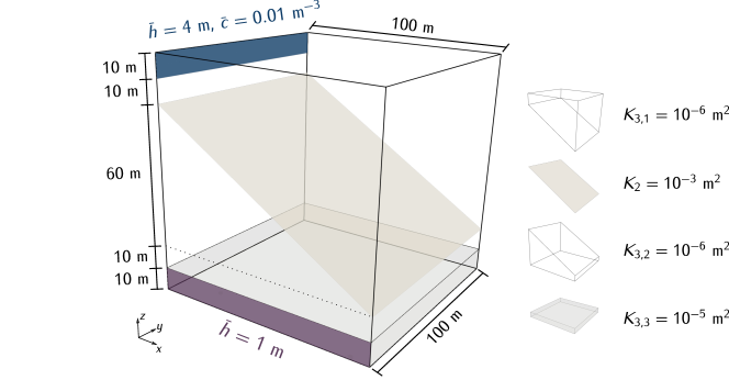
Figure 1: Conceptual model and geometrical description of the domain for Case 1 of Subsection 5.1.

The domain $\Omega$ is a cube-shaped region ($0\text{\,}\mathrm{m}\text{/}$, $100\text{\,}\mathrm{m}\text{/}$) $\times$ ($0\text{\,}\mathrm{m}\text{/}$, $100\text{\,}\mathrm{m}\text{/}$) $\times$ ($0\text{\,}\mathrm{m}\text{/}$, $100\text{\,}\mathrm{m}\text{/}$) which is crossed by a planar fracture, $\Omega_{2}$, with a thickness of $1\text{\times}{10}^{-2}\text{\,}\mathrm{m}\text{/}$. The matrix domain consists of subdomains $\Omega_{3,1}$ above the fracture and $\Omega_{3,2}$ and $\Omega_{3,3}$ below. The subdomain $\Omega_{3,3}$ represents a heterogeneity within the rock matrix. Inflow into the system occurs through a narrow band defined by $\{$0\text{\,}\mathrm{m}\text{/}$\}\times($0\text{\,}\mathrm{m}\text{/}$,$100\text{\,}\mathrm{m}\text{/}$)\times($90\text{\,}\mathrm{m}\text{/}$,$100\text{\,}\mathrm{m}\text{/}$)$. Similarly, the outlet is a narrow band defined by $($0\text{\,}\mathrm{m}\text{/}$,$100\text{\,}\mathrm{m}\text{/}$)\times\{$0\text{\,}\mathrm{m}\text{/}$\}\times($0\text{\,}\mathrm{m}\text{/}$,$10\text{\,}\mathrm{m}\text{/}$)$.

At the inlet and outlet bands, we impose the hydraulic head $h_{in}=$4\text{\,}\mathrm{m}\text{/}$$ and $h_{out}=$1\text{\,}\mathrm{m}\text{/}$$ respectively, and $c_{in}=$1\text{\times}{10}^{-2}\text{\,}{\mathrm{m}}^{-3}\text{/}$$ is set at the inlet for the transport problem. All remaining parts of the boundary are assigned no-flow conditions. The parameters for conductivity, porosity, and aperture are listed in Table 3 together with the overall simulation time and time-step size.

Matrix hydraulic conductivity $K_{3,1}$, $K_{3,2}$	$1\text{\times}{10}^{-6}$$\bm{I}$	$\mathrm{m}\text{/}\mathrm{s}$
Matrix hydraulic conductivity $K_{3,3}$	$1\text{\times}{10}^{-5}$$\bm{I}$	$\mathrm{m}\text{/}\mathrm{s}$
Fracture effective tangential hydraulic conductivity $K_{2}$	$1\text{\times}{10}^{-3}$$\bm{I}$	$\mathrm{m}^{2}\mathrm{/}\mathrm{s}$
Fracture effective normal hydraulic conductivity $\kappa_{2}$	$20$	$\text{/}\mathrm{s}$
Matrix porosity $\phi_{3,1},\phi_{3,2}$	$2\text{\times}{10}^{-1}$
Matrix porosity $\phi_{3,3}$	$2.5\text{\times}{10}^{-1}$
Fracture porosity $\phi_{2}$	$4\text{\times}{10}^{-1}$
Fracture cross-sectional length $\epsilon_{2}$	$1\text{\times}{10}^{-2}$	$\mathrm{m}\text{/}$
Total simulation time	$1\text{\times}{10}^{9}$	$\mathrm{s}\text{/}$
Time-step $\Delta t$	$1\text{\times}{10}^{7}$	$\mathrm{s}\text{/}$

Table 3: Parameters used in Case 1 of Subsection 5.1.

5.1.2 Results

Three different simulations were carried out with approximately $1$k, $10$k and $100$k cells for the 3d domain. The precise number of cells and degrees of freedom for each method are listed in Table 7 and will be discussed in Subsection 5.1.2. We compare the methods on the basis of computed pressure head and concentration, plotted along prescribed lines. The first comparison, represented in Subsection 5.1.2, depicts the hydraulic head along a line crossing the 3d matrix domain, while the solutions reported in 5.1.2 and 5.1.2 visualize the matrix and fracture concentration along lines at the final simulation time. Plots in Subsection 5.1.2 and 5.1.2 depict integrated matrix and fracture concentrations over time, respectively. Finally, we compare concentration fluxes across the outlet over time in Subsection 5.1.2.

Hydraulic Head Over Line

Figure 2 depicts the hydraulic head $h_{3}$ in the matrix along the line $\left($0\text{\,}\mathrm{m}\text{/}$,$100\text{\,}\mathrm{m}\text{/}$,$100\text{\,}\mathrm{m}\text{/}$\right)$-$\left($100\text{\,}\mathrm{m}\text{/}$,$0\text{\,}\mathrm{m}\text{/}$,$0\text{\,}\mathrm{m}\text{/}$\right)$. Each plot corresponds to one of the three refinement levels.

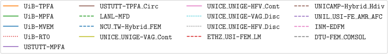
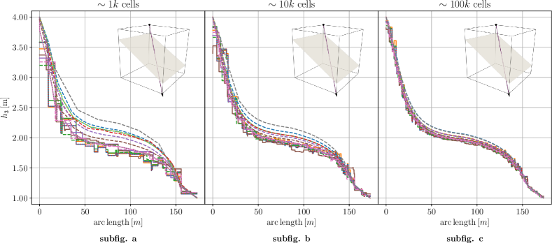
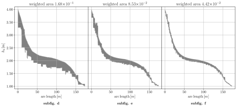
Figure 2: Case 1 of Subsection 5.1. On the top, the hydraulic head $h_{3}$ in the matrix over the line $\left($0\text{\,}\mathrm{m}\text{/}$,$100\text{\,}\mathrm{m}\text{/}$,$100\text{\,}\mathrm{m}\text{/}$\right)$ - $\left($100\text{\,}\mathrm{m}\text{/}$,$0\text{\,}\mathrm{m}\text{/}$,$0\text{\,}\mathrm{m}\text{/}$\right)$ for three refinements (coarse to fine). On the bottom, the area between the 10th and 90th percentiles for three refinements (coarse to fine) and data. Results of Subsection 5.1.2.

At the coarsest level of around 1000 cells, all methods already show reasonable agreement. As expected, differences between the methods decrease with increasing refinement level. We remark that two classes of methods can be distinguished in these plots. First, the methods that use cellwise constant values exhibit staircase-like patterns. On the other hand, methods using nodal values are interpolated within each cell and yield a smoother appearance.

To quantify the differences between the participating methods and their convergence behavior over all refinement levels, we calculate and visualize the spread of the associated data sets. For that purpose, the solution values are evaluated at 1000 evenly distributed points along the considered line. At each such point, the mean as well as the 10th and 90th percentiles are determined. Each plot in the bottom row of Figure 2 visualizes the area between the 10th and 90th percentiles over the evaluation points. The number in the picture title corresponds to that area divided by the area under the mean curve. Convergence between the methods can clearly be observed.

Matrix Concentration Over Line

The pictures at the top of Figure 3 illustrate the concentration $c_{3}$ in the matrix at the final simulation time along the line $\left($0\text{\,}\mathrm{m}\text{/}$,$100\text{\,}\mathrm{m}\text{/}$,$100\text{\,}\mathrm{m}\text{/}$\right)$-$\left($100\text{\,}\mathrm{m}\text{/}$,$0\text{\,}\mathrm{m}\text{/}$,$0\text{\,}\mathrm{m}\text{/}$\right)$, again for the different refinement levels.

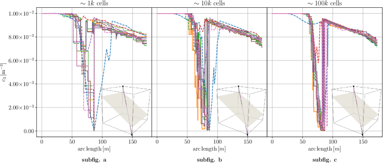
Figure 3: Case 1 of Subsection 5.1. On the top, concentration $c_{3}$ in the matrix, at the final simulation time, along the line $\left($0\text{\,}\mathrm{m}\text{/}$,$100\text{\,}\mathrm{m}\text{/}$,$100\text{\,}\mathrm{m}\text{/}$\right)$ - $\left($100\text{\,}\mathrm{m}\text{/}$,$0\text{\,}\mathrm{m}\text{/}$,$0\text{\,}\mathrm{m}\text{/}$\right)$ for three refinements (coarse to fine). On the bottom, area between the 10th and 90th percentiles for three refinements (coarse to fine) and data. Results of Subsection 5.1.2.

We observe a similar behavior to that in 5.1.2 in the sense that the differences between most of the methods decrease with increasing refinement level. However, two methods show more pronounced deviations from the rest: ETHZ_USI-FEM_LM exhibits oscillations that can be attributed to the fact that the employed algebraic flux correction stabilization scheme does not suppress all spurious oscillations. The NCU_TW-Hybrid_FEM does not capture the curve behavior at all. The obviously larger spread in the results is visualized more explicitly in the bottom row of Figure 3. As a result, the convergence is much slower compared to Subsection 5.1.2.

Fracture Concentration Over Line

Figure 4 shows the concentration $c_{2}$ within the fracture at the final simulation time along the line $\left($0\text{\,}\mathrm{m}\text{/}$,$100\text{\,}\mathrm{m}\text{/}$,$80\text{\,}\mathrm{m}\text{/}$\right)$-$\left($100\text{\,}\mathrm{m}\text{/}$,$0\text{\,}\mathrm{m}\text{/}$,$20\text{\,}\mathrm{m}\text{/}$\right)$.

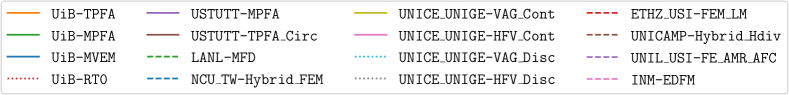
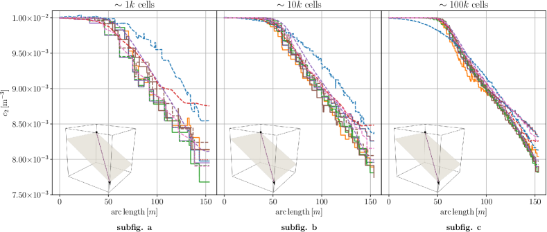
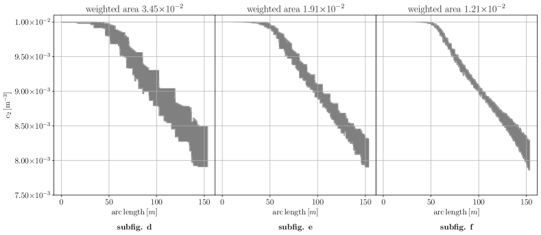
Figure 4: Case 1 of Subsection 5.1. On the top, concentration $c_{2}$ within the fracture, at the final simulation time, along the line $\left($0\text{\,}\mathrm{m}\text{/}$,$100\text{\,}\mathrm{m}\text{/}$,$80\text{\,}\mathrm{m}\text{/}$\right)$-$\left($100\text{\,}\mathrm{m}\text{/}$,$0\text{\,}\mathrm{m}\text{/}$,$20\text{\,}\mathrm{m}\text{/}$\right)$ for three refinements (coarse to fine). On the bottom, area between the 10th and 90th percentiles for three refinements (coarse to fine) and data. Results of Subsection 5.1.2.

Again, almost all methods appear to converge with increasing refinement. NCU_TW-Hybrid_FEM and UiB-TPFA exhibit the largest deviations over all refinement levels. Close to the outlet boundary, ETHZ_USI-FEM_LM yields rather different values than the rest of the methods, but its tendency to approach the other methods with refinement can be observed clearly. Additionally, INM-EDFM still shows considerably different results on the right boundary for the highest refinement level. Looking at the bottom row of Figure 4, the convergence behavior of the spread is better than that of the matrix concentration reported in Subsection 5.1.2, yet worse than for the matrix hydraulic head in Subsection 5.1.2.

Integrated Matrix Concentration Over Time

Unlike the first three plots in 5.1.2-5.1.2, Figure 5 illustrates an integrated quantity over time, namely, the integrated matrix concentration $\int_{\Omega_{3,3}}\phi_{3}c_{3}\,\mathrm{d}x$.

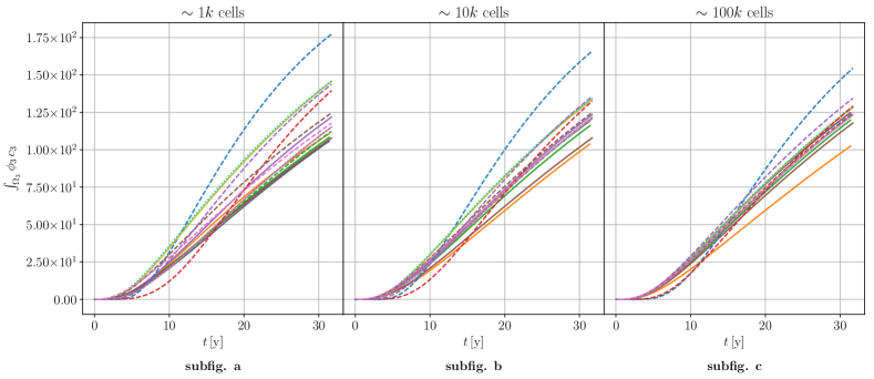
Figure 5: Case 1 of Subsection 5.1. integrated matrix concentration $\int_{\Omega_{3,3}}\phi_{3}c_{3}\,\mathrm{d}x$ for three refinements (coarse to fine). Results of Subsection 5.1.2.

Correspondingly, all curves appear much smoother than above. Over the three refinement levels, most methods again exhibit decreasing differences between each other. Remarkably, the UiB-TPFA shows a pronounced underestimation that increases over time. This can be explained by the inconsistency of the employed two-point flux approximation on the tetrahedral grids. Additionally, the NCU_TW-Hybrid_FEM and ETHZ_USI-FEM_LM again exhibit larger differences.

Integrated Fracture Concentration Over Time

Analogously, the integrated fracture concentration $\int_{\Omega_{2}}\varepsilon_{2}\phi_{2}c_{2}\,\mathrm{d}x$ for each time-step is visualized in Figure 6.

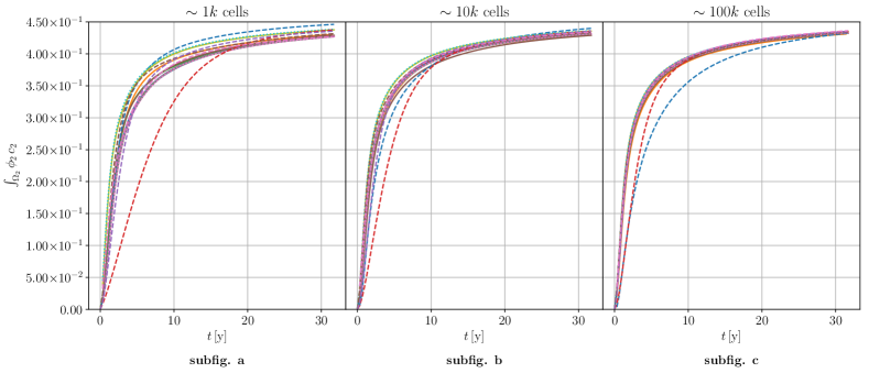
Figure 6: Case 1 of Subsection 5.1. Integrated fracture concentration $\int_{\Omega_{2}}\varepsilon_{2}\phi_{2}c_{2}\,\mathrm{d}x$ over time for three refinements (coarse to fine). Results of Subsection 5.1.2.

The behavior of the curves is generally different from that reported in Subsection 5.1.2, as the fracture fills up completely before the final simulation time. Here, the UiB-TPFA is in line with the other methods whereas the NCU_TW-Hybrid_FEM and ETHZ_USI-FEM_LM both deviate from the majority.

Concentration Flux Across the Outlet Over Time

Finally, Figure 7 depicts the integrated concentration flux across the outlet boundary over time.

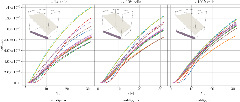
Figure 7: Case 1 of Subsection 5.1. Integrated flux of $c$ across the outlet boundary over time for three refinements (coarse to fine). Results of Subsection 5.1.2.

Compared to the results in Subsection 5.1.2, the agreement between the methods appears to be poorer. In particular, the two-point flux approximation of the UiB-TPFA results in an underestimation similar to that reported in 5.1.2. Again, ETHZ_USI-FEM_LM and NCU_TW-Hybrid_FEM yield considerably different results at all refinement levels.

Computational Cost

Indicators for the computational costs associated with the different methods are presented in Table 7. Most methods satisfy the prescribed numbers of elements. The most notable exception is given by the NCU_TW-Hybrid_FEM, where six to ten times as many tetrahedral elements have been employed, to compensate for the fact that the degrees of freedom are associated with the vertices. The number of vertices are in line with the prescribed cell numbers. The relations of the number of degrees of freedom to the number of cells vary considerably between the different schemes, reflecting the characteristics from Table 2. The lowest such numbers are for the purely head- and vertex-based schemes on tetrahedrons for the NCU_TW-Hybrid_FEM and DTU-FEM_COMSOL, while the highest ones result from the schemes that have head and velocity values as degrees of freedom. Additionally, the ratios of the number of nonzero entries to the number of degrees of freedom exhibit a large variability, ranging from approximately 5 (TPFA on tetrahedrons) to 30 (MPFA schemes with only head degrees of freedom).

5.2 Case 2: Regular Fracture Network

Benchmark case designers: A. Fumagalli and I. Stefansson
Benchmark case coordinators: W. Boon and D. Gläser

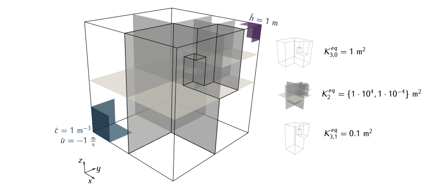
Figure 8: Representation of the domain ($\Omega_{3}=\left(0,1\right)^{3}$) and the fractures for Case 2 of Subsection 5.2. The inlet and outlet boundaries are colored in blue and purple, respectively, and on the right side, the permeability distributions among $\Omega_{3}$ and $\Omega_{2}$ are illustrated.

5.2.1 Description

The second benchmark is a three-dimensional analog of the two-dimensional test case 4.1 from the benchmark study [2]. The domain is given by the unit cube $\Omega=\left($0\text{\,}\mathrm{m}\text{/}$,$1\text{\,}\mathrm{m}\text{/}$\right)^{3}$ and contains 9 regularly oriented fractures, as illustrated in Figure 8. The boundary $\partial\Omega$ is decomposed into three parts, each corresponding to a chosen boundary condition (see Figure 8). First, $\partial\Omega_{h}=\{(x,y,z)\in\partial\Omega:x,y,z>$0.875\text{\,}\mathrm{m}\text{/}$\}$ is the part of the boundary on which we impose $\overline{h}=$1\text{\,}\mathrm{m}\text{/}$$. Second, we set a flux boundary condition on $\partial\Omega_{in}=\{(x,y,z)\in\partial\Omega:x,y,z<$0.25\text{\,}\mathrm{m}\text{/}$\}$ by imposing $\overline{u}=$-1\text{\,}\mathrm{m}\text{/}\mathrm{s}$$. On the remainder of the boundary of $\Omega$, we impose no-flow conditions.

Two variants of the test case are considered: Case 2.1 has highly conductive fractures and Case 2.2 has blocking fractures. In both cases, different hydraulic conductivities are prescribed in the following matrix subregions:

$$\Omega_{3,0}= \ \Omega_{3}\setminus\Omega_{3,1}$$

$$\Omega_{3,1}= \ \{(x,y,z)\in\Omega_{3}:x>$0.5\text{\,}\mathrm{m}\text{/}$\cap y<$0.5\text{\,}\mathrm{m}\text{/}$\}$$

$$\cup\{(x,y,z)\in\Omega_{3}:x>$0.75\text{\,}\mathrm{m}\text{/}$\cap$0.5\text{\,}\mathrm{m}\text{/}$<y<$0.75\text{\,}\mathrm{m}\text{/}$\cap z>$0.5\text{\,}\mathrm{m}\text{/}$\}$$

$$\cup\{(x,y,z)\in\Omega_{3}:$0.625\text{\,}\mathrm{m}\text{/}$<x<$0.75\text{\,}\mathrm{m}\text{/}$\cap$0.5\text{\,}\mathrm{m}\text{/}$<y<$0.625\text{\,}\mathrm{m}\text{/}$\cap$0.5\text{\,}\mathrm{m}\text{/}$<z<$0.75\text{\,}\mathrm{m}\text{/}$\}.$$

For an illustration of these regions, we refer to the right part of Figure 8. A complete overview of the parameters used in this test case is given in Table 4.

Finally, for the transport problem, we impose unitary concentration at the inflow boundary $\partial\Omega_{in}$.

	Case 2.1		Case 2.2
Matrix hydraulic conductivity $K_{3}|_{\Omega_{3,0}}$	$\bm{I}$	$\mathrm{m}\text{/}\mathrm{s}$	$\bm{I}$	$\mathrm{m}\text{/}\mathrm{s}$
Matrix hydraulic conductivity $K_{3}|_{\Omega_{3,1}}$	$1\text{\times}{10}^{-1}$$\bm{I}$	$\mathrm{m}\text{/}\mathrm{s}$	$1\text{\times}{10}^{-1}$$\bm{I}$	$\mathrm{m}\text{/}\mathrm{s}$
Fracture effective tangential hydraulic conductivity $K_{2}$	$\bm{I}$	${\mathrm{m}}^{2}\text{/}\mathrm{s}$	$1\text{\times}{10}^{-8}$$\bm{I}$	${\mathrm{m}}^{2}\text{/}\mathrm{s}$
Fracture effective normal hydraulic conductivity $\kappa_{2}$	$2\text{\times}{10}^{8}$	$\text{/}\mathrm{s}$	$2$	$\text{/}\mathrm{s}$
Intersection effective tangential hydraulic conductivity $K_{1}$	$1\text{\times}{10}^{-4}$	${\mathrm{m}}^{3}\text{/}\mathrm{s}$	$1\text{\times}{10}^{-12}$	${\mathrm{m}}^{3}\text{/}\mathrm{s}$
Intersection effective normal hydraulic conductivity $\kappa_{1}$	$2\text{\times}{10}^{4}$	$\mathrm{m}\text{/}\mathrm{s}$	$2\text{\times}{10}^{-4}$	$\mathrm{m}\text{/}\mathrm{s}$
Intersection effective normal hydraulic conductivity $\kappa_{0}$	$2$	${\mathrm{m}}^{2}\text{/}\mathrm{s}$	$2\text{\times}{10}^{-8}$	${\mathrm{m}}^{2}\text{/}\mathrm{s}$
Matrix porosity $\phi_{3}$	$1\text{\times}{10}^{-1}$		$1\text{\times}{10}^{-1}$
Fracture porosity $\phi_{2}$	$9\text{\times}{10}^{-1}$		$1\text{\times}{10}^{-2}$
Intersection porosity $\phi_{1}$	$9\text{\times}{10}^{-1}$		$1\text{\times}{10}^{-2}$
Fracture cross-sectional length $\epsilon_{2}$	$1\text{\times}{10}^{-4}$	$\mathrm{m}\text{/}$	$1\text{\times}{10}^{-4}$	$\mathrm{m}\text{/}$
Intersection cross-sectional area $\epsilon_{1}$	$1\text{\times}{10}^{-8}$	${\mathrm{m}}^{2}\text{/}$	$1\text{\times}{10}^{-8}$	${\mathrm{m}}^{2}\text{/}$
Intersection cross-sectional volume $\epsilon_{0}$	$1\text{\times}{10}^{-12}$	${\mathrm{m}}^{3}\text{/}$	$1\text{\times}{10}^{-12}$	${\mathrm{m}}^{3}\text{/}$
Total simulation time	$2.5\text{\times}{10}^{-1}$	$\mathrm{s}\text{/}$
Time-step $\Delta t$	$2.5\text{\times}{10}^{-3}$	$\mathrm{s}\text{/}$

Table 4: Parameters used in Case 2 of Subsection 5.2.

5.2.2 Results

The results were collected for a sequence of 3 simulations by discretizing the 3d domain using approximately $500$, $4$k, and $32$k cells. The number of cells and degrees of freedom used by the participating methods are reported in Table 8. In the following, we discuss the results on the basis of line profiles of the hydraulic head in the 3d matrix as well as plots of the average concentrations within specified subregions of the 3d matrix.

Hydraulic Head Over Line

Figure 9 shows the hydraulic head $h_{3}$ plotted along the diagonal line segment (0, 0, 0)-(1, 1, 1) for all grid refinements and for both Case 2.1 and Case 2.2. In the case of conductive fractures the spread decreases significantly upon grid refinement, although some noticeable differences still prevail for the finest grid.

In the case of blocking fractures, the highest discrepancies are shown by the schemes that assume continuity of the hydraulic head across the fractures. As expected, these methods cannot capture the jump in the hydraulic head present in this test case. On the other hand, the remaining schemes seem to approach the same solution. We observe that the UNICE_UNIGE-VAG_Disc and the UNIL_USI-FE_AMR_AFC produce slightly lower and the UNICAMP-Hybrid_Hdiv scheme slightly higher hydraulic heads, but the deviations tend to diminish with increasing grid refinement.

The UNICE_UNIGE-VAG_Cont and UNICE_UNIGE-VAG_Disc methods incorporate Dirichlet boundary conditions on the vertices rather than on faces. This may explain, in part, the deviations in hydraulic head observed on coarse meshes for these methods. As expected, these differences decrease with mesh refinement. For the UNIL_USI-FE_AMR_AFC method, the differences might come from the representation of the fractures, which have the same spatial dimension as the background matrix. In particular, each fracture consists of a layer of elements that is refined at least twice by using adaptive mesh refinement.

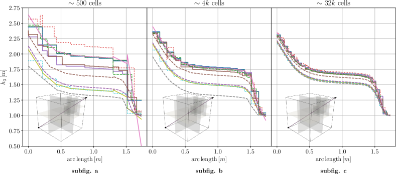
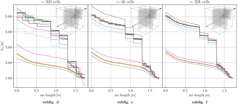
Figure 9: Case 2 of Subsection 5.2. Plots of the hydraulic head $h_{3}$ along the line $(0,0,0)$ - $(1,1,1)$ for the different refinement levels (grid refinement increases from left to right) for the case of conductive fractures (Case 2.1, upper row) and blocking fractures (Case 2.2, lower row). Results of Subsection 5.2.2.

Mean Matrix Concentration Over Time

The second comparison in Case 2 concerns the solution of the transport equation over time. These solutions are computed only on the second level of mesh refinement, i.e., using approximately $4000$ cells. For the simulation of the transport model, the upwind scheme is employed for all methods except UNIL_USI-FE_AMR_AFC and ETHZ_USI-FEM_LM, which employ a finite element discretization with an algebraic flux correction [26].

The top of Figure 10 depicts the temporal evolution of the mean tracer concentrations in three matrix regions for the case of highly conductive fractures. These regions were selected to form a representative illustration of the spread between the schemes. It can be seen that the majority of the schemes produce rather low concentrations in the first region, on the order of $2.5\text{\,}\mathrm{\char 37\relax}\text{/}$ at the final simulation time. In contrast, the ETHZ_USI-FEM_LM and the UNIL_USI-FE_AMR_AFC schemes produce significantly higher concentrations with values above $10\text{\,}\mathrm{\char 37\relax}\text{/}$ at the end of the simulation. In general, the temporal evolution of the concentrations in these three regions agrees very well among the majority of participating schemes, while the ETHZ_USI-FEM_LM and the UNIL_USI-FE_AMR_AFC schemes show significant deviations. These might be related to the flow discretization methods, but could also be affected by the different discretization that is employed for the transport discretization related to these methods, and, for UNIL_USI-FE_AMR_AFC, also the underlying equidimensional model.

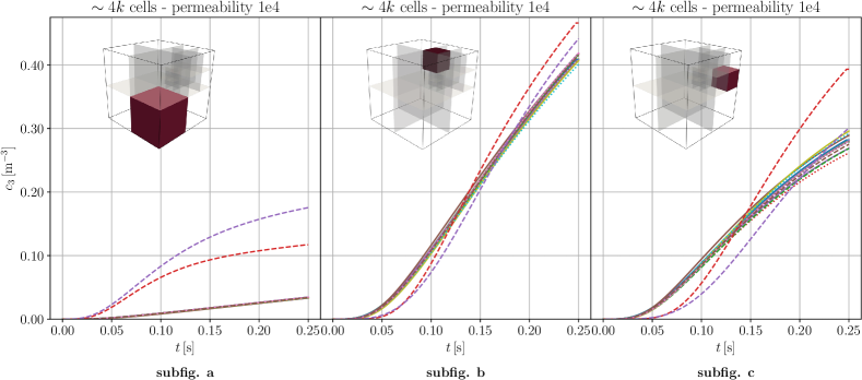
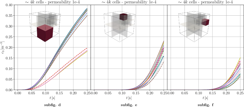
Figure 10: Case 2 of Subsection 5.2. On the top, temporal evolution of the average tracer concentration in matrix regions $1$, $10$ and $11$ (from left to right) for the case of conductive fractures (Case 2.1). On the bottom, temporal evolution of the average tracer concentration in the matrix regions $1$, $10$ and $11$ (from left to right) for the case of blocking fractures (Case 2.2). Results of Subsection 5.2.2.

For the case of blocking fractures, the concentrations in the same matrix regions are illustrated in the bottom row of Figure 10. In general, a larger spread of the computed concentrations can be observed. For the first region, the schemes that assume continuity of the hydraulic head produce significantly lower concentrations, while the remaining schemes produce solutions that agree rather well. However, for the second and third regions, the concentrations at the final simulation time show a widespread among all participating schemes.

As a general trend, it can be observed that the differences in computed concentrations increase with time. Additionally, differences increase with the regions’ distance from the inflow boundary. As expected, for the case of conductive fractures, the differences are smaller than in the case of blocking fractures.

5.3 Case 3: Network with Small Features

Benchmark case designers: E. Keilegavlen and I. Stefansson
Benchmark case coordinator: I. Stefansson and A. Fumagalli

5.3.1 Description

This test case is designed to probe accuracy in the presence of small geometric features, which may cause trouble for conforming meshing strategies. The domain is the box $\Omega=($0\text{\,}\mathrm{m}\text{/}$,$1\text{\,}\mathrm{m}\text{/}$)\times($0\text{\,}\mathrm{m}\text{/}$,$2.25\text{\,}\mathrm{m}\text{/}$)\times($0\text{\,}\mathrm{m}\text{/}$,$1\text{\,}\mathrm{m}\text{/}$)$, containing eight fractures (see Figure 11).

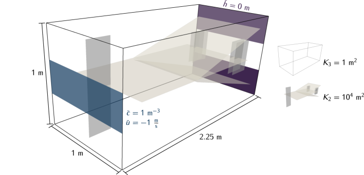
Figure 11: Representation of the fractures and the outline of the domain for Case 3 of Subsection 5.3.

We define the inlet and outlet boundaries as follows:

$$\partial\Omega_{N} =\partial\Omega\setminus(\partial\Omega_{in}\cup\partial\Omega_{out})$$

$$\partial\Omega_{in} =($0\text{\,}\mathrm{m}\text{/}$,$1\text{\,}\mathrm{m}\text{/}$)\times\{$0\text{\,}\mathrm{m}\text{/}$\}\times($1\text{/}3\text{\,}\mathrm{m}\text{/}$,$2\text{/}3\text{\,}\mathrm{m}\text{/}$)$$

$$\partial\Omega_{out} =\partial\Omega_{out,0}\cup\partial\Omega_{out,1}$$

$$\partial\Omega_{out,0} =($0\text{\,}\mathrm{m}\text{/}$,$1\text{\,}\mathrm{m}\text{/}$)\times\{$2.25\text{\,}\mathrm{m}\text{/}$\}\times($0\text{\,}\mathrm{m}\text{/}$,$1\text{/}3\text{\,}\mathrm{m}\text{/}$)$$

$$\partial\Omega_{out,1} =($0\text{\,}\mathrm{m}\text{/}$,$1\text{\,}\mathrm{m}\text{/}$)\times\{$2.25\text{\,}\mathrm{m}\text{/}$\}\times($2\text{/}3\text{\,}\mathrm{m}\text{/}$,$1\text{\,}\mathrm{m}\text{/}$)$$

The boundary conditions for flow are homogeneous Dirichlet conditions on $\partial\Omega_{out}$, uniform unit inflow on $\partial\Omega_{in}$, so that $\int_{\partial\Omega_{in}}\bm{u}_{3}\cdot\bm{n}dS=-1/3$ ${\mathrm{m}}^{3}\text{/}\mathrm{s}$, and homogeneous Neumann conditions on $\partial\Omega_{N}$. For the transport problem, we consider a homogeneous initial condition and as boundary condition a unit concentration at $\partial\Omega_{in}$. A complete overview of the parameters used in Case 3 is given in Table 5.

Matrix hydraulic conductivity $K_{3}$	$\bm{I}$	$\mathrm{m}\text{/}\mathrm{s}$
Fracture effective tangential hydraulic conductivity $K_{2}$	$1\text{\times}{10}^{2}$$\bm{I}$	${\mathrm{m}}^{2}\text{/}\mathrm{s}$
Fracture effective normal hydraulic conductivity $\kappa_{2}$	$2\text{\times}{10}^{6}$	$\text{/}\mathrm{s}$
Intersection effective tangential hydraulic conductivity $K_{1}$	$1$	${\mathrm{m}}^{3}\text{/}\mathrm{s}$
Intersection effective normal hydraulic conductivity $\kappa_{1}$	$2\text{\times}{10}^{4}$	$\mathrm{m}\text{/}\mathrm{s}$
Matrix porosity $\phi_{3}$	$2\text{\times}{10}^{-1}$
Fracture porosity $\phi_{2}$	$2\text{\times}{10}^{-1}$
Intersection effective porosity $\phi_{1}$	$2\text{\times}{10}^{-1}$
Fracture cross-sectional length $\epsilon_{2}$	$1\text{\times}{10}^{-2}$	$\mathrm{m}\text{/}$
Intersection cross-sectional area $\epsilon_{1}$	$1\text{\times}{10}^{-4}$	${\mathrm{m}}^{2}\text{/}$
Total simulation time	$1$	$\mathrm{s}\text{/}$
Time-step $\Delta t$	$1\text{\times}{10}^{-2}$	$\mathrm{s}\text{/}$

Table 5: Parameters used in Case 3 of Subsection 5.3.

5.3.2 Results

Similar to the previous cases, we compare the methods on the basis of a) the hydraulic head of the matrix domain along two lines, b) the integrated fracture concentration over time, c) the fluxes out of the domain and d) computational cost. Two different simulations with approximately $30$k and $150$k cells for the 3d domain were performed. It was seen as infeasible to include one more level of refinement for all methods. However, refined versions of the USTUTT-MPFA with up to approximately $1\text{\times}{10}^{6}$ matrix cells were produced. At this stage, there were no noticeable differences between solutions on different grids, and the finest solution was included as a reference solution.

Hydraulic Head Over Line

Figure 12 shows the profile of the hydraulic head $h_{3}$ in the matrix along the line $\left($0.5\text{\,}\mathrm{m}\text{/}$,$1.1\text{\,}\mathrm{m}\text{/}$,$0\text{\,}\mathrm{m}\text{/}$\right)$-$\left($0.5\text{\,}\mathrm{m}\text{/}$,$1.1\text{\,}\mathrm{m}\text{/}$,$1\text{\,}\mathrm{m}\text{/}$\right)$. This shows considerable differences between the methods for both refinement levels.

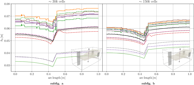
Figure 12: Case 3 of Subsection 5.3. Hydraulic head $h_{3}$ in the matrix over the line $\left($0.5\text{\,}\mathrm{m}\text{/}$,$1.1\text{\,}\mathrm{m}\text{/}$,$0\text{\,}\mathrm{m}\text{/}$\right)$-$\left($0.5\text{\,}\mathrm{m}\text{/}$,$1.1\text{\,}\mathrm{m}\text{/}$,$1\text{\,}\mathrm{m}\text{/}$\right)$ for the coarse (left) and fine (right) grid. The solid black line shows the solution obtained with the USTUTT-MPFA scheme on a grid with approximately $1\text{\times}{10}^{6}$ matrix cells. Results of Subsection 5.3.2.

However, the agreement is better for the second refinement level, where most of the methods are within a relative hydraulic head range of approximately $10\text{\,}\mathrm{\char 37\relax}\text{/}$. The UNICE_UNIGE-VAG_Disc, UNICE_UNIGE-VAG_Cont, DTU-FEM_COMSOL, and UNIL_USI-FE_AMR_AFC methods show the highest discrepancies in these plots, but the deviation from the reference solution decreases significantly with higher refinement. The significant difference between the refinements may indicate that the small features of the fracture network geometry are not adequately resolved, at least not by the coarser grids. This is in line with the purpose of the test case.

Mean Fracture Concentration Over Time

Data were reported for the integrated concentration $\overline{c_{2}}=\int_{\Omega_{2,i}}c_{2}/|\Omega_{2,i}|$ on each fracture $i$ throughout the simulation. There is a general agreement between the methods, with the method of ETHZ_USI-FEM_LM showing some deviations for some of the fractures. As an example, Figure 13 shows the plots for both refinement levels for fracture number 3, demonstrating limited difference between the refinement levels.

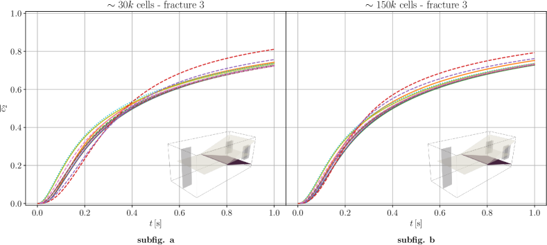
Figure 13: Case 3 of Subsection 5.3. Mean concentration within fracture number 3 throughout the simulation time for the coarse (left) and fine (right) grid. Results of Subsection 5.3.2.

Boundary Fluxes

The total outflow $\overline{u}_{out}=\int_{\partial\Omega_{out}}\bm{u}_{3}\cdot\bm{n}dS$ and the proportion exiting over $\partial\Omega_{out,0}$, i.e., $r_{out}=\int_{\partial\Omega_{out,0}}\bm{u}_{3}\cdot\bm{n}dS/\overline{u}_{out}$, are shown in Figure 14. When compared to the prescribed inflow of $-1\text{/}3\text{\,}{\mathrm{m}}^{3}\text{/}\mathrm{s}$, the $\overline{u}_{out}$ values reveal a small lack of volume conservation for ETHZ_USI-FEM_LM, but the method improves for the finer grid. The ratio $r_{out}$ provides an indication of whether the flux fields agree. The ratios generally agree well with the refined USTUTT-MPFA, except for the ETHZ_USI-FEM_LM method, which does not approach the reference value for the finest grid.

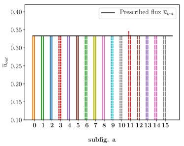
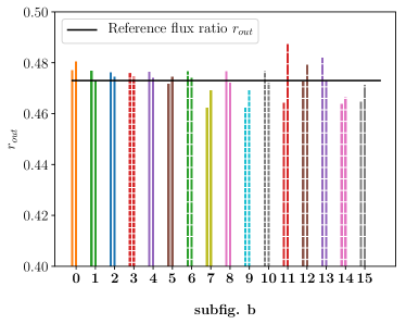
Figure 14: Case 3 of Subsection 5.3. Total outflux (left) and ratio exiting over $\partial\Omega_{out,0}$ (right). The bar pairs correspond to the coarse and fine grid, while the reference solution is indicated by the horizontal line. Results of Subsection 5.3.2.

Computational Cost

Based on the data presented in Table 9, we note that the UNIL_USI-FE_AMR_AFC applies $68$k and $~{}203$k cells for the cases where $30$k and $150$k cells were prescribed, respectively. The rest of the methods are well within $10\text{\,}\mathrm{\char 37\relax}\text{/}$ of the prescribed values. As for the other test cases, there are significant variations in the number of degrees of freedom and nonzero matrix entries related to the design of the methods.

5.4 Case 4: Field Case

Benchmark case designers: E. Keilegavlen and A. Fumagalli
Benchmark case coordinator: E. Keilegavlen

5.4.1 Description

The geometry of the fourth case is based on a postprocessed outcrop from the island of Algerøyna, outside Bergen, Norway, and is a subset of the fracture network presented in [52]. From the outcrop, 52 fractures were selected, extruded in the vertical direction and then cut by a bounding box. The resulting network has 106 fracture intersections, and multiple fractures intersect the domain boundary. The simulation domain is the box $\Omega=($-500\text{\,}\mathrm{m}\text{/}$,$350\text{\,}\mathrm{m}\text{/}$)\times($100\text{\,}\mathrm{m}\text{/}$,$1500\text{\,}\mathrm{m}\text{/}$)\times($-100\text{\,}\mathrm{m}\text{/}$,$500\text{\,}\mathrm{m}\text{/}$)$. The fracture geometry is depicted in Figure 15.

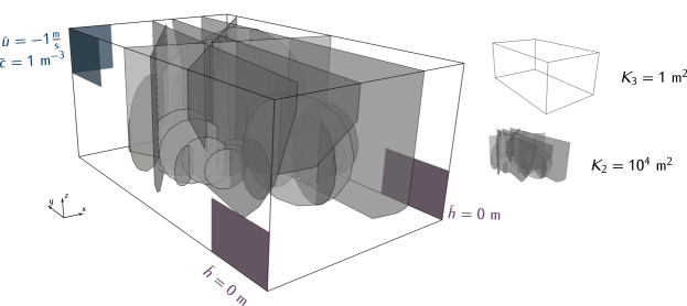
Figure 15: Case 4 of Subsection 5.4. Representation of the fractures and the outline of the domain. Inlet boundaries are shown in blue, outlets in purple.

The inlet and outlet boundaries are defined as follows:

$$\partial\Omega_{N} =\partial\Omega\setminus(\partial\Omega_{in}\cup\partial\Omega_{out}),$$

$$\partial\Omega_{in} =\partial\Omega_{in,0}\cup\partial\Omega_{in,1},\qquad\partial\Omega_{out}=\partial\Omega_{out,0}\cup\partial\Omega_{out,1},$$

$$\partial\Omega_{in,0} =($-500\text{\,}\mathrm{m}\text{/}$,$-200\text{\,}\mathrm{m}\text{/}$)\times\{$1500\text{\,}\mathrm{m}\text{/}$\}\times($300\text{\,}\mathrm{m}\text{/}$,$500\text{\,}\mathrm{m}\text{/}$),$$

$$\partial\Omega_{in,1} =\{$-500\text{\,}\mathrm{m}\text{/}$\}\times($1200\text{\,}\mathrm{m}\text{/}$,$1500\text{\,}\mathrm{m}\text{/}$)\times($300\text{\,}\mathrm{m}\text{/}$,$500\text{\,}\mathrm{m}\text{/}$),$$

$$\partial\Omega_{out,0} =\{$-500\text{\,}\mathrm{m}\text{/}$\}\times($100\text{\,}\mathrm{m}\text{/}$,$400\text{\,}\mathrm{m}\text{/}$)\times($-100\text{\,}\mathrm{m}\text{/}$,$100\text{\,}\mathrm{m}\text{/}$),$$

$$\partial\Omega_{out,1} =\{$350\text{\,}\mathrm{m}\text{/}$\}\times($100\text{\,}\mathrm{m}\text{/}$,$400\text{\,}\mathrm{m}\text{/}$)\times($-100\text{\,}\mathrm{m}\text{/}$,$100\text{\,}\mathrm{m}\text{/}$).$$

The boundary conditions for flow are homogeneous Dirichlet conditions on $\partial\Omega_{out}$, uniform unit inflow on $\partial\Omega_{in}$, so that $\int_{\partial\Omega_{in}}\bm{u}_{3}\cdot\bm{n}dS=$-1.2\text{\times}{10}^{5}\text{\,}{\mathrm{m}}^{3}\text{/}\mathrm{s}$$, and homogeneous Neumann conditions on $\partial\Omega_{N}$. For the transport problem, we consider a homogeneous initial condition, with a unit concentration at $\partial\Omega_{in}$. The parameters for conductivity, porosity and aperture are given in Table 6, as is the total simulation time and time-step size.

Matrix hydraulic conductivity $K_{3}$	$\bm{I}$	$\mathrm{m}\text{/}\mathrm{s}$
Fracture effective tangential hydraulic conductivity $K_{2}$	$1\text{\times}{10}^{2}$$\bm{I}$	${\mathrm{m}}^{2}\text{/}\mathrm{s}$
Fracture effective normal hydraulic conductivity $\kappa_{2}$	$2\text{\times}{10}^{6}$	$\text{/}\mathrm{s}$
Intersection effective tangential hydraulic conductivity $K_{1}$	$1$	${\mathrm{m}}^{3}\text{/}\mathrm{s}$
Intersection effective normal hydraulic conductivity $\kappa_{1}$	$2\text{\times}{10}^{4}$	$\mathrm{m}\text{/}\mathrm{s}$
Matrix porosity $\phi_{3}$	$2\text{\times}{10}^{-1}$
Fracture porosity $\phi_{2}$	$2\text{\times}{10}^{-1}$
Intersection porosity $\phi_{1}$	$2\text{\times}{10}^{-1}$
Fracture cross-sectional length $\epsilon_{2}$	$1\text{\times}{10}^{-2}$	$\mathrm{m}\text{/}$
Intersection cross-sectional area $\epsilon_{1}$	$1\text{\times}{10}^{-4}$	${\mathrm{m}}^{2}\text{/}$
Total simulation time	$5\text{\times}{10}^{3}$	$\mathrm{s}\text{/}$
Time-step $\Delta t$	$5\text{\times}{10}^{1}$	$\mathrm{s}\text{/}$

Table 6: Parameter used in Case 4 of Subsection 5.4.

Because of the complex network geometry, grid refinement studies were considered infeasible and the benchmark specified the usage of a single grid. A Gmsh [53] configuration file, was provided to assist participants with geometry processing and meshing. The use of this predefined grid was optional, but the number of 3d cells should be approximately 260k.

5.4.2 Results

Results were reported for 14 schemes. The two methods that participated in Case 3, which is closest in geometric complexity, but not in Case 4, are INM-EDFM and UNIL_USI-FE_AMR_AFC. The participating methods are compared in terms of a) hydraulic head of the matrix domain along two lines, b) time series of concentrations in selected fractures and c) computational cost.

Hydraulic Head

Figure 16 shows the hydraulic head along the two specified lines, together with the spread of the reported results.

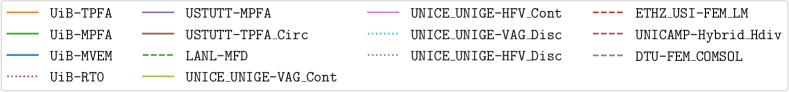
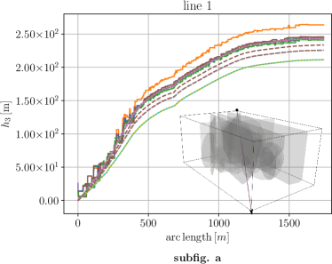
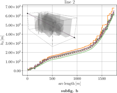
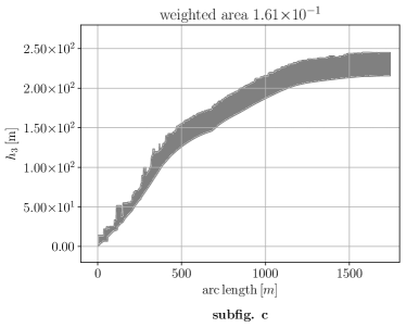
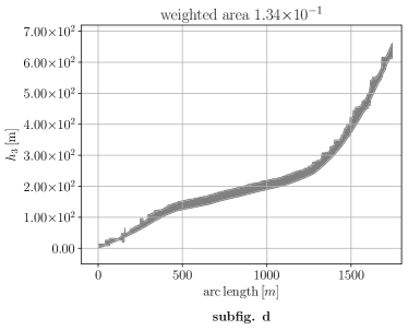
Figure 16: Case 4 of Subsection 5.4. Hydraulic head profiles across the domain. Left: Profile from outlet $\partial\Omega_{out,0}$ towards the opposite corner. Right: Profile from outlet $\partial\Omega_{out,1}$ towards $\partial\Omega_{in}$. Results of Subsection 5.4.2.

Both lines start in points at the outflow boundaries where the hydraulic head is set to 0; the first line ends far away from the inlet, while the second ends at the inlet boundary. For the first line there are noticeable deviations for some of the solutions: The UiB-TPFA scheme predicts a significantly higher hydraulic head drop, likely caused by the inconsistency of the scheme. Conversely, the UNICE_UNIGE-VAG_Disc and UNICE_UNIGE-VAG_Cont methods underestimate the drop in hydraulic head compared to the average of the reported results, while there is only minor disagreement among the other methods. On the second line, the UiB-TPFA scheme overestimates the drop in hydraulic head over the domain, while the other methods are in very good agreement.

Concentration Plots

The quality of the flux field is measured by the time series of average concentrations in the fracture planes, with good agreement among most of the methods. Figure 17 shows the time evolution of concentration for three of the fractures, numbers 15, 45 and 48, which show the largest differences between the methods.

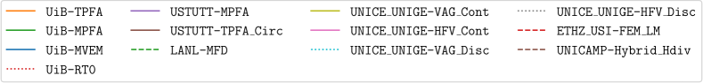
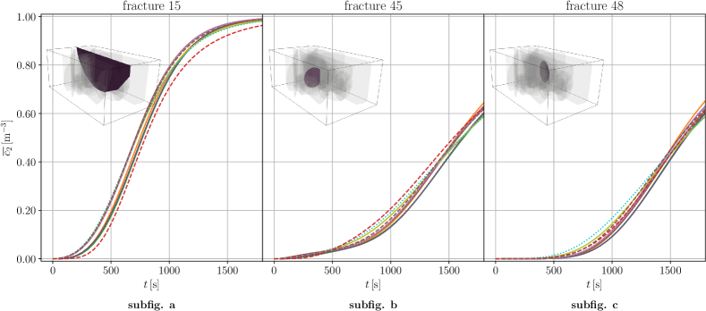
Figure 17: Case 4 of Subsection 5.4. Mean concentration over time in three selected fractures with identification 15, 45, and 48. Results of Subsection 5.4.2.

The results produced by the ETHZ_USI-FEM_LM deviate slightly from the other methods on two of these figures, while UNICE_UNIGE-VAG_Disc also shows a slight deviation for one of the figures.

Computational Cost

Measures for the computational cost of the participating methods are given in Table 10. Most of the groups used the provided mesh file. The UNICAMP-Hybrid_Hdiv method used a grid with only approximately 40% of the cells in the provided grid. DTU-FEM_COMSOL employed almost seven times more 3d cells for its nodal-based method, yielding a number of degrees of freedom that is in the lower half with respect to all participating methods. As in the previous test cases, there are significant differences in the number of unknowns and nonzero matrix elements among the methods.

6 Summary of Results

The performance of each method for all test cases is indicated in Figure 18. We also list the main points emerging from the discussion of the results in Section 5:

1. Of the 17 schemes that participated in at least one of the test cases, 14 presented simulation results on all four cases.

2. Cases 3 and 4 pose the highest demands on the methods in terms of geometrical complexity. Taken together, the cases point to the challenges inherent to DFM simulations and indicate the methods’ robustness in this respect.

3. Not unexpectedly, fractures that act as barriers cause trouble for the methods that assume a continuous hydraulic head over the fracture, as seen in Case 2. Blocking fractures are outside the intended range of validity for these models, and alternative approaches should be sought for those cases.

4. Out of the 17 schemes, one is not mass conservative. There are no signs of the lack of conservation in the reported concentration fields, likely due to successful postprocessing of the flux fields. Nevertheless, for most of the test cases, the concentration fields reported by the nonconforming mesh method ETHZ_USI-FEM_LM deviate from the other reported results.

5. The well-known inconsistency of the widely used two-point flux approximation is manifested in the underestimation of permeability in the hydraulic head results reported for UiB-TPFA. The USTUTT-TPFA_Circ method circumvents this inconsistency by locating the hydraulic head values at the circumcenters of the tetrahedrons. However, this poses additional restrictions on the mesh.

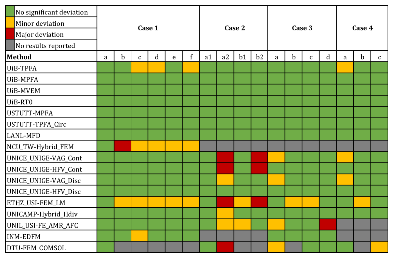
Figure 18: Summary of the performance of all methods.

7 Conclusion

This paper has presented a set of benchmark cases for the simulation of Darcy flow in three-dimensional fractured porous media. The suite consists of one case with a single fracture, one case with 9 fractures and setups with conductive and blocking fractures, one case with 8 fractures designed to emphasize complex geometric details, and finally a case with 52 fractures, based on a real fracture network. The metrics employed to measure discretization performance are (1) the profiles of the hydraulic head, (2) the quality of the flux field measured by simulation of passive tracers and (3) the computational cost as indicated by the number of degrees of freedom and matrix sparsity pattern. A total of 17 methods participated in the benchmark, spanning a wide range of discretization approaches for fractured media. Although it was not possible to identify one approach as superior, the benchmark uncovered important differences between the methods. The high number of participating methods and research groups proves that simulations in 3d media are fully feasible for a wide range of schemes and research codes. For further development of discretization methods, 3d cases should therefore become a natural complement to the more traditional 2d simulation results.

All data used in the benchmark can be found in the online repository https://git.iws.uni-stuttgart.de/benchmarks/fracture-flow-3d.git. This includes the specification of benchmark case parameters, geometries, ready-made mesh generation files, applied metrics, and the results of all participating methods. Additionally, Python scripts and Jupyter notebooks are provided which enable the reproduction of the result figures as well as the comparison of new computational results. Therefore, we expect that the present work can serve as a reference point for the further development of discretization methods for fractured porous media.

8 Acknowledgments

I. Berre, A. Fumagalli, E. Keilegavlen, and I. Stefansson were supported by Norwegian Research Council grants 250223, 244129/E20 and 267908/E20. The contribution of S. Burbulla was funded by the Deutsche Forschungsgemeinschaft (DFG, German Research Foundation) – Project Number 327154368 – SFB 1313. P. Devloo was supported by Fapesp grant No 2017/15736-3, ANP/Petrobras grant No 2014/00090-2 and CNPq grant No 310369/2006-1. O. Duran was supported by ANP/Petrobras grant No 2014/00090-2. M. Favino was supported by the Swiss National Science Foundation (SNSF) grant PZ00P2_180112. M. Nestola and P.Zulian were supported by the SCCER-SoE and the Pasc Project FASTER. C.F. Ni and I.H. Lee were partially funded by Institute of Nuclear Energy Research under grant NL1050288 and by Ministry of Science and Technology under grant MOST 108-2116-M-008-004- and MOST 106-2116-M-008-014-. K. Nikitin and R. Yanbarisov were supported by Moscow Center for Fundamental and Applied Mathematics (agreement with the Ministry of Education and Science of the Russian Federation No. 075-15-2019-1624). P. Schädle thanks the Werner Siemens Foundation for their endowment of the Geothermal Energy and Geofluids group at the Institute of Geophysics, ETH Zurich.

9 Appendix

9.1 Measures of Computational Cost

This section provides three indicators related to computational cost: the number of cells (0d-3d), the number of degrees of freedom and the number of nonzero matrix entries. There is one table for each test case with data of all the participating methods at all refinement levels. For the equidimensional UNIL_USI-FE_AMR_AFC method, the cells listed as “0d-2d cells” are also three-dimensional cells that correspond to the fractures (“2d”), intersections of fractures (“1d”) and intersections of such intersections (“0d”).

Method	Refinement	0d cells	1d cells	2d cells	3d cells	dofs	nnz
UiB-TPFA	0	0	0	112	1022	1358	6008
	1	0	0	756	9438	11706	53904
	2	0	0	4576	98311	112039	533547
UiB-MPFA	0	0	0	112	1022	1358	62200
	1	0	0	756	9438	11706	672454
	2	0	0	4576	98311	112039	7481237
UiB-MVEM	0	0	0	112	1022	3905	24435
	1	0	0	756	9438	33651	222927
	2	0	0	4576	98311	326561	2259630
UiB-RT0	0	0	0	112	1022	3905	24435
	1	0	0	756	9438	33651	222927
	2	0	0	4576	98311	326561	2259623
USTUTT-MPFA	0	0	0	100	1000	1100	22626
	1	0	0	400	9600	10000	227354
	2	0	0	3600	108000	111600	2731104
USTUTT-TPFA_Circ	0	0	0	193	3400	3593	17373
	1	0	0	448	9085	9533	46505
	2	0	0	2582	104578	107160	530224
LANL-MFD	0	0	0	100	1000	4400	51720
	1	0	0	400	8000	34840	390840
	2	0	0	1600	64000	267280	3035280
NCU_TW-Hybrid_FEM	0	0	0	625	9572	1840	25539
	1	0	0	2453	65934	11537	169937
	2	0	0	22262	638332	104581	1603776
UNICE_UNIGE-VAG_Cont	0	0	0	81	1134	1511	34085
	1	0	0	361	10108	11721	288933
	2	0	0	1849	103544	111233	2877105
UNICE_UNIGE-HFV_Cont	0	0	0	81	1134	3870	39060
	1	0	0	361	10108	32319	340879
	2	0	0	1849	103544	320221	3454921
UNICE_UNIGE-VAG_Disc	0	0	0	81	1134	1943	43519
	1	0	0	361	10108	13483	328867
	2	0	0	1849	103544	119771	3073987
UNICE_UNIGE-HFV_Disc	0	0	0	81	1134	4077	40041
	1	0	0	361	10108	33231	345135
	2	0	0	1849	103544	324779	3475475
ETHZ_USI-FEM_LM	0	0	0	120	1000	1617	38834
	1	0	0	480	10115	12714	335023
	2	0	0	1920	93150	103470	2775270
UNICAMP-Hybrid_Hdiv	0	0	0	526	1054	5968	114924
	1	0	0	2884	10589	62164	1249536
	2	0	0	15052	100273	604019	12448629
UNIL_USI-FE_AMR_AFC	0	0	0	720	540	1857	49417
	1	0	0	10880	38180	56947	1545935
	2	0	0	39520	108671	579837	16878449
INM-EDFM	0	0	0	140	1000	1140	7666
	1	0	0	720	10000	10720	73364
	2	0	0	3800	100000	103800	719292
DTU-FEM_COMSOL	0	0	0	0	1006	259	3082
	1	0	0	0	10091	1931	26771
	2	0	0	0	100014	17850	258202

Table 7: Computational cost indicators for Case 1

Method	Refinement	0d cells	1d cells	2d cells	3d cells	dofs	nnz
UiB-TPFA	0	27	90	252	512	1820	8253
	1	27	180	1008	4096	8074	43513
	2	27	360	4032	32768	46622	281717
UiB-MPFA	0	27	90	252	512	1820	8609
	1	27	180	1008	4096	8074	44984
	2	27	360	4032	32768	46622	287565
UiB-MVEM	0	27	90	252	512	4706	20795
	1	27	180	1008	4096	24862	118620
	2	27	360	4032	32768	161414	806000
UiB-RT0	0	27	72	226	612	3970	21687
	1	27	159	1192	5339	24727	153263
	2	27	270	4536	39157	148245	980955
USTUTT-MPFA	0	0	0	284	843	1127	42060
	1	0	0	686	3076	3762	207260
	2	0	0	4578	38877	43455	2918322
USTUTT-TPFA_Circ	0	0	0	312	978	1290	7488
	1	0	0	1206	4286	5492	31402
	2	0	0	4578	38877	43455	226201
LANL-MFD	0	0	0	434	628	2758	23246
	1	0	0	1736	5024	18610	150314
	2	0	0	6944	40192	134812	1062572
UNICE_UNIGE-VAG_Cont	0	0	0	252	512	974	22324
	1	0	0	1008	4096	5902	143470
	2	0	0	4032	32768	39908	1014088
UNICE_UNIGE-HFV_Cont	0	0	0	252	512	2223	22599
	1	0	0	1008	4096	15048	157980
	2	0	0	4032	32768	109368	1172592
UNICE_UNIGE-VAG_Disc	0	0	0	252	512	2102	46348
	1	0	0	1008	4096	10223	238891
	2	0	0	4032	32768	56607	1390939
UNICE_UNIGE-HFV_Disc	0	0	0	252	512	2730	24138
	1	0	0	1008	4096	17076	164148
	2	0	0	4032	32768	117480	1197288
ETHZ_USI-FEM_LM	0	0	0	1212	512	3159	67183
	1	0	0	1212	4096	7343	182793
	2	0	0	1212	32768	38367	1036960
UNICAMP-Hybrid_Hdiv	0	27	69	534	923	6018	123312
	1	27	90	1896	3912	23988	479322
	2	27	249	10744	38742	236868	4830288
UNIL_USI-FE_AMR_AFC	0	1331	2787	6513	1745	16283	410491
	1	1331	5211	20673	8129	45257	1180333
	2	1331	10059	72033	47553	161805	4274281
DTU-FEM_COMSOL	0	0	0	0	550	129	1561
	1	0	0	0	3881	836	10900
	2	0	0	0	32147	6060	84954

Table 8: Computational cost indicators for Case 2

Method	Refinement	0d cells	1d cells	2d cells	3d cells	dofs	nnz
UiB-TPFA	0	0	50	4305	31644	44786	207295
	1	0	86	13731	138446	180024	849349
UiB-MPFA	0	0	50	4305	31644	44786	2596061
	1	0	86	13731	138446	180024	11196843
UiB-MVEM	0	0	50	4305	31644	120696	818151
	1	0	86	13731	138446	496032	3438098
UiB-RT0	0	0	50	4305	31644	120696	818151
	1	0	86	13731	138446	496032	3438098
USTUTT-MPFA	0	0	0	4321	31942	36263	2459195
	1	0	0	12147	131488	143635	10157331
USTUTT-TPFA_Circ	0	0	0	4321	31942	36263	191147
	1	0	0	12147	131488	143635	745375
LANL-MFD	0	0	0	5617	21056	75878	607730
	1	0	0	22468	168448	555887	4367379
UNICE_UNIGE-VAG_Cont	0	0	0	4321	31870	10213	130781
	1	0	0	7711	150083	35485	479105
UNICE_UNIGE-HFV_Cont	0	0	0	4321	31870	71708	504872
	1	0	0	7711	150083	319175	2206691
UNICE_UNIGE-VAG_Disc	0	0	0	4321	31870	23302	400876
	1	0	0	7711	150083	59187	966849
UNICE_UNIGE-HFV_Disc	0	0	0	4321	31870	80538	532114
	1	0	0	7711	150083	335599	2259971
ETHZ_USI-FEM_LM	0	0	0	750	29295	33270	899809
	1	0	0	3000	150930	163430	4421700
UNICAMP-Hybrid_Hdiv	0	0	38	5580	24351	153519	3180847
	1	0	51	23607	162773	994243	20600135
UNIL_USI-FE_AMR_AFC	0	0	3877	323779	68386	86594	1206048
	1	0	3877	323779	547088	148993	2202947
INM-EDFM	0	0	0	4036	29952	33988	240398
	1	0	0	10732	149760	160492	1133364
DTU-FEM_COMSOL	0	0	0	0	30984	5641	80669
	1	0	0	0	150524	30379	469447
USTUTT-MPFA-refined	5	0	0	49428	980212	1029640	75207825

Table 9: Computational cost indicators for Case 3

Method	0d cells	1d cells	2d cells	3d cells	dofs	nnz
UiB-TPFA	0	1601	52618	259409	424703	1950313
UiB-MPFA	0	1601	52618	259409	424703	22953336
UiB-MVEM	0	1601	52618	259409	1082740	7342691
UiB-RT0	0	1601	52618	259409	1082740	7342691
USTUTT-MPFA	0	0	52618	259420	312038	21227071
USTUTT-TPFA_Circ	0	0	52618	259420	312038	1721932
LANL-MFD	0	0	52070	260417	783158	7953396
UNICE_UNIGE-VAG_Cont	0	0	52070	260431	95930	1237714
UNICE_UNIGE-HFV_Cont	0	0	52070	260431	600561	4349901
UNICE_UNIGE-VAG_Disc	0	0	52070	260431	252326	4497980
UNICE_UNIGE-HFV_Disc	0	0	52070	260431	704813	4663105
ETHZ_USI-FEM_LM	0	0	52618	212040	223532	5817930
UNICAMP-Hybrid_Hdiv	0	938	24853	94294	629065	13233581
DTU-FEM_COMSOL	0	0	0	1860063	319489	4709565

Table 10: Computational cost indicators for Case 4

References

- [1] I. Berre, F. Doster, E. Keilegavlen, Flow in fractured porous media: A review of conceptual models and discretization approaches, Transport in Porous Media 130 (1) (2019) 215–236. doi:10.1007/s11242-018-1171-6.
- [2] B. Flemisch, I. Berre, W. Boon, A. Fumagalli, N. Schwenck, A. Scotti, I. Stefansson, A. Tatomir, Benchmarks for single-phase flow in fractured porous media, Advances in Water Resources 111 (2018) 239–258. doi:10.1016/j.advwatres.2017.10.036.
- [3] A. Arrarás, F. J. Gaspar, L. Portero, C. Rodrigo, Mixed-dimensional geometric multigrid methods for single-phase flow in fractured porous media, SIAM Journal on Scientific Computing 41 (5) (2019) B1082–B1114. doi:10.1137/18M1224751.
- [4] A. Budisa, X. Hu, Block Preconditioners for Mixed-dimensional Discretization of Flow in Fractured Porous Media, arXiv e-prints (2019) 1905.13513.
- [5] A. Budisa, W. Boon, X. Hu, Mixed-dimensional auxiliary space preconditioners, arXiv preprint arXiv:1910.04704 (2019).
- [6] Fumagalli, Alessio, Keilegavlen, Eirik, Dual virtual element methods for discrete fracture matrix models, Oil Gas Sci. Technol. - Rev. IFP Energies nouvelles 74 (2019) 41. doi:10.2516/ogst/2019008.
- [7] M. Köppel, V. Martin, J. Jaffré, J. E. Roberts, A Lagrange multiplier method for a discrete fracture model for flow in porous media, Computational Geosciences 23 (2) (2019) 239–253. doi:10.1007/s10596-018-9779-8.
- [8] M. Köppel, V. Martin, J. E. Roberts, A stabilized lagrange multiplier finite-element method for flow in porous media with fractures, GEM - International Journal on Geomathematics 10 (1) (2019) 7. doi:10.1007/s13137-019-0117-7.
- [9] L. H. Odsæter, T. Kvamsdal, M. G. Larson, A simple embedded discrete fracture–matrix model for a coupled flow and transport problem in porous media, Computer Methods in Applied Mechanics and Engineering 343 (2019) 572–601. doi:10.1016/j.cma.2018.09.003.
- [10] P. Schädle, P. Zulian, D. Vogler, S. R. Bhopalam, M. G. Nestola, A. Ebigbo, R. Krause, M. O. Saar, 3d non-conforming mesh model for flow in fractured porous media using lagrange multipliers, Computers & Geosciences 132 (2019) 42–55. doi:10.1016/j.cageo.2019.06.014.
- [11] I. Stefansson, I. Berre, E. Keilegavlen, Finite-volume discretisations for flow in fractured porous media, Transport in Porous Media 124 (2) (2018) 439–462. doi:10.1007/s11242-018-1077-3.
- [12] I. Berre, W. Boon, B. Flemisch, A. Fumagalli, D. Gläser, E. Keilegavlen, A. Scotti, I. Stefansson, A. Tatomir, Call for participation: Verification benchmarks for single-phase flow in three-dimensional fractured porous media, arXiv e-prints (2018) 1809.06926.
- [13] P. A. Raviart, J. M. Thomas, A mixed finite element method for 2-nd order elliptic problems, in: I. Galligani, E. Magenes (Eds.), Mathematical Aspects of Finite Element Methods, Springer Berlin Heidelberg, 1977, p. 292–315. doi:10.1007/BFb0064470.
- [14] F. Brezzi, M. Fortin, Mixed and Hybrid Finite Element Methods, Vol. 15 of Computational Mathematics, Springer Verlag, Berlin, 1991.
- [15] J. E. Roberts, J.-M. Thomas, Mixed and hybrid methods, in: P. G. Ciarlet, J. L. Lions (Eds.), Handbook of numerical analysis, Vol. II, North-Holland, Amsterdam, 1991, pp. 523–639. doi:10.1016/S1570-8659(05)80041-9.
- [16] A. Ern, J.-L. Guermond, Theory and Practice of Finite Elements, Vol. 159 of Applied mathematical sciences, Springer, 2004. doi:10.1007/978-1-4757-4355-5.
- [17] C. Alboin, J. Jaffré, J. E. Roberts, X. Wang, C. Serres, Domain decomposition for some transmission problems in flow in porous media, in: Z. Chen, R. E. Ewing, Z.-C. Shi (Eds.), Numerical treatment of multiphase flows in porous media (Beijing, 1999), Vol. 552 of Lecture Notes in Phys., Springer, Berlin, 2000, pp. 22–34. doi:10.1007/3-540-45467-5_2.
- [18] I. Faille, E. Flauraud, F. Nataf, S. Pégaz-Fiornet, F. Schneider, F. Willien, A New Fault Model in Geological Basin Modelling. Application of Finite Volume Scheme and Domain Decomposition Methods, in: Finite volumes for complex applications, III (Porquerolles, 2002), Hermes Sci. Publ., Paris, 2002, pp. 529–536.
- [19] P. Angot, A model of fracture for elliptic problems with flux and solution jumps, Comptes Rendus Mathematique 337 (6) (2003) 425–430. doi:10.1016/S1631-073X(03)00300-5.
- [20] V. Martin, J. Jaffré, J. E. Roberts, Modeling Fractures and Barriers as Interfaces for Flow in Porous Media, SIAM J. Sci. Comput. 26 (5) (2005) 1667–1691. doi:10.1137/S1064827503429363.
- [21] C. D’Angelo, A. Scotti, A mixed finite element method for Darcy flow in fractured porous media with non-matching grids, Mathematical Modelling and Numerical Analysis 46 (02) (2012) 465–489. doi:10.1051/m2an/2011148.
- [22] A. Fumagalli, A. Scotti, An Efficient XFEM Approximation of Darcy Flows in Arbitrarily Fractured Porous Media, Oil and Gas Sciences and Technologies - Revue d’IFP Energies Nouvelles 69 (4) (2014) 555–564. doi:10.2516/ogst/2013192.
- [23] N. Schwenck, B. Flemisch, R. Helmig, B. Wohlmuth, Dimensionally reduced flow models in fractured porous media: crossings and boundaries, Computational Geosciences 19 (6) (2015) 1219–1230. doi:10.1007/s10596-015-9536-1.
- [24] B. Flemisch, A. Fumagalli, A. Scotti, A review of the xfem-based approximation of flow in fractured porous media, in: G. Ventura, E. Benvenuti (Eds.), Advances in Discretization Methods: Discontinuities, Virtual Elements, Fictitious Domain Methods, Vol. 12 of SEMA SIMAI Springer Series, Springer International Publishing, Cham, 2016, pp. 47–76. doi:10.1007/978-3-319-41246-7_3.
- [25] W. M. Boon, J. M. Nordbotten, I. Yotov, Robust discretization of flow in fractured porous media, SIAM Journal on Numerical Analysis 56 (4) (2018) 2203–2233. doi:10.1137/17M1139102.
- [26] D. Kuzmin, R. Löhner, S. Turek (Eds.), Flux-corrected transport: principles, algorithms, and applications, Springer, 2012. doi:10.1007/978-94-007-4038-9.
- [27] E. Keilegavlen, R. Berge, A. Fumagalli, M. Starnoni, I. Stefansson, J. Varela, I. Berre, PorePy: An Open-Source Software for Simulation of Multiphysics Processes in Fractured Porous Media, arXiv e-prints (2019) 1908.09869.
- [28] J. M. Nordbotten, W. M. Boon, A. Fumagalli, E. Keilegavlen, Unified approach to discretization of flow in fractured porous media, Computational Geosciences 23 (2) (2019) 225–237. doi:10.1007/s10596-018-9778-9.
- [29] https://github.com/pmgbergen/porepy (2019).
- [30] https://github.com/pmgbergen/arXiv_1809_06926 (2019).
- [31] B. Flemisch, M. Darcis, K. Erbertseder, B. Faigle, A. Lauser, K. Mosthaf, S. Müthing, P. Nuske, A. Tatomir, M. Wolff, R. Helmig, DuMux: DUNE for multi- Phase, Component, Scale, Physics, … flow and transport in porous media, Advances in Water Resources 34 (2011) 1102–1112. doi:10.1016/j.advwatres.2011.03.007.
- [32] https://git.iws.uni-stuttgart.de/dumux-repositories/dumux (2019).
- [33] https://git.iws.uni-stuttgart.de/dumux-pub/berre2019a (2019).
- [34] K. Lipnikov, G. Manzini, M. Shashkov, Mimetic finite difference method, Journal of Computational Physics 257 (2014) 1163 – 1227. doi:10.1016/j.jcp.2013.07.031.
- [35] https://github.com/amanzi (2019).
- [36] I.-H. Lee, C.-F. Ni, Fracture-based modeling of complex flow and CO2 migration in three-dimensional fractured rocks, Computers & Geosciences 81 (2015) 64 – 77. doi:10.1016/j.cageo.2015.04.012.
- [37] I.-H. Lee, C.-F. Ni, F.-P. Lin, C.-P. Lin, C.-C. Ke, Stochastic modeling of flow and conservative transport in three-dimensional discrete fracture networks, Hydrology and Earth System Sciences (2019) 19–34doi:10.5194/hess-23-19-2019.
- [38] K. Brenner, M. Groza, C. Guichard, G. Lebeau, R. Masson, Gradient discretization of hybrid dimensional darcy flows in fractured porous media, Numerische Mathematik 134 (3) (2016) 569–609. doi:10.1007/s00211-015-0782-x.
- [39] K. Brenner, J. Hennicker, R. Masson, P. Samier, Gradient discretization of hybrid-dimensional Darcy flow in fractured porous media with discontinuous pressures at matrix–fracture interfaces, IMA Journal of Numerical Analysis 37 (3) (2016) 1551–1585. doi:10.1093/imanum/drw044.
- [40] M. Köppel, V. Martin, J. Jaffré, J. E. Roberts, A lagrange multiplier method for a discrete fracture model for flow in porous media, Computational Geosciences 23 (2) (2019) 239–253. doi:10.1007/s10596-018-9779-8.
- [41] R. Krause, P. Zulian, A parallel approach to the variational transfer of discrete fields between arbitrarily distributed unstructured finite element meshes, SIAM Journal on Scientific Computing 38 (2016) C307–C333. doi:10.1137/15M1008361.
-
[42]
P. Zulian, A. Kopanicáková, M. C. G. Nestola, A. Fink, N. Fadel,
V. Magri, T. Schneider, E. Botter,
Utopia: A C++ embedded
domain specific language for scientific computing. Git repository (2016).
URL https://bitbucket.org/zulianp/utopia - [43] P. Devloo, W. Teng, C.-S. Zhang, Multiscale hybrid-mixed finite element method for flow simulation in fractured porous media, Computer Modeling in Engineering & Sciences 119 (1) (2019) 145–163. doi:10.32604/cmes.2019.04812.
- [44] O. Durán, P. R. Devloo, S. M. Gomes, F. Valentin, A multiscale hybrid method for darcy’s problems using mixed finite element local solvers, Computer Methods in Applied Mechanics and Engineering 354 (2019) 213 – 244. doi:10.1016/j.cma.2019.05.013.
- [45] https://github.com/labmec/HDiv/tree/master/HDiv_Benchmarks (2019).
- [46] M. Favino, J. Hunziker, E. Caspari, B. Quital, K. Holliger, R. Krause, Fully-automated adaptive mesh refinement for media embedding complex heterogeneities: Application to poroelastic fluid pressure diffusion, submitted (2019).
- [47] K. Nikitin, R. Yanbarisov, Monotone embedded discrete fractures method for flows in porous media, J. Comp. Appl. Math. 364 (2020). doi:10.1016/j.cam.2019.112353.
- [48] https://www.comsol.com/release/5.4 (2019).
- [49] I. Berre, W. M. Boon, B. Flemisch, A. Fumagalli, D. Gläser, E. Keilegavlen, A. Scotti, I. Stefansson, A. Tatomir, K. Brenner, S. Burbulla, P. Devloo, O. Duran, M. Favino, J. Hennicker, I.-H. Lee, K. Lipnikov, R. Masson, K. Mosthaf, M. G. C. Nestola, C.-F. Ni, K. Nikitin, P. Schädle, D. Svyatskiy, R. Yanbarisov, P. Zulian, Data repository of this work, https://git.iws.uni-stuttgart.de/benchmarks/fracture-flow-3d.git (2020).
-
[50]
W. Zielke, R. Helmig, K. Krohn, H. Shao, J. Wollrath,
Discrete modelling of transport processes in fractured porous
rock, in: 7th ISRM Congress, 1991, pp. 57–60.
URL https://www.onepetro.org/conference-paper/ISRM-7CONGRESS-1991-013 - [51] C. Barlag, R. Hinkelmann, R. Helmig, W. Zielke, Adaptive methods for modelling transport processes in fractured subsurface systems, 3rd International Conference on Hydroscience and Engineering, Cottbus (1998).
- [52] A. Fumagalli, E. Keilegavlen, S. Scialò, Conforming, non-conforming and non-matching discretization couplings in discrete fracture network simulations, Journal of Computational Physics 376 (2019) 694–712. doi:10.1016/j.jcp.2018.09.048.
- [53] C. Geuzaine, J.-F. Remacle, Gmsh: A 3-d finite element mesh generator with built-in pre- and post-processing facilities, International Journal for Numerical Methods in Engineering 79 (11) (2009) 1309–1331. doi:10.1002/nme.2579.