Neutron scattering off Weyl semimetals

Abstract

We present how to detect type-$1$ Weyl nodes in a material by inelastic neutron scattering. Such an experiment first of all allows one to determine the dispersion of the Weyl fermions. We extend the reasoning to produce a quantitative test of the Weyl equation taking into account realistic anisotropic properties. These anisotropies are mostly contained in the form of the emergent magnetic moment of the excitations, which determines how they couple to the neutrons. Although there are many material parameters, we find several quantitative predictions that are universal and demonstrate that the excitations are described by solutions to the Weyl equation. The anisotropic coupling between electrons and neutrons implies that even fully unpolarized neutrons can reveal the spin-momentum locking of the Weyl fermions because the neutrons will couple to some components of the Weyl fermion pseudospin more strongly. On the other hand, in an experiment with polarized neutrons, the scattered neutron beam remains fully polarized in a direction that varies as a function of momentum transfer (within the range of validity of the Weyl equation). This allows measurement of the chirality of Weyl fermions for inversion symmetric nodes. Furthermore, we estimate that the scattering rate may be large enough for such experiments to be practical; in particular, the magnetic moment may be larger than the ordinary Bohr magneton, compensating for a small density of states.

I Introduction

The Weyl equation, first applied in high-energy physics to describe neutrinos, has recently been connected to condensed matter physics, where it describes materials whose electronic excitations have a strong coupling between spin and orbital degrees of freedom. In experimentsXu et al. (2015); Yang et al. (2015); Lv et al. (2015) guided by band structure calculationsWan et al. (2011); Weng et al. (2015); Huang et al. (2015), Weyl fermions have recently been realized in the context of Weyl semimetals (WSM) in crystalline solids, photonic crystalsLu et al. (2015), and magnon bandsMook et al. (2016); Li et al. (2016); Li et al. (2017).

Except for establishing magnetic structureLiu et al. (2017); Guo et al. (2014); Nakajima et al. (2015), spin dynamicsItoh et al. (2016), and probing magnon excitationsYao et al. (2018); Shivam et al. (2017), neutron scattering has by and large been absent in revealing the physics in topological semimetalsArmitage et al. (2018); Bernevig et al. (2018). WSMs, however, are characterized by the property that their excitations are spin-momentum locked. This indicates that inelastic neutron scattering (INS) could measure these as it is a probe well-suited for measuring magnetic properties of excitations. However, it has long been known, that INS is a technique that has severe difficulties probing electronic excitations due to kinematic restrictions, form factor and low density of states at the Fermi level. For normal metallic systems, the cross-section intensity was predictedSilver (1984) to be as low as $10^{-4}-10^{-3}\;{\rm mb/meV\,sr\,f.u.}$. At first glance, the prospects of probing excitations in WSMs seem worse, since the cross-section should be limited by the small density of states at a Weyl point. However, the coupling of the neutron to Weyl fermions has a contribution from orbital currents in addition to the usual form factor that determines the rate of neutron scattering. This can be large enough to compensate for the small density of states. As a proof of concept, we employ a toy model to estimate the cross-section with this coupling included; with some optimistic assumptions, the cross-section can be as large as $10^{-2}\;{\rm mb/meV\,sr\,f.u.}$, which is similar to the rates of scattering associated with other spin$-\frac{1}{2}$ related phenomena, that have been observedGoremychkin et al. (2018); Vignolle et al. (2007); Walters et al. (2009); Fujita et al. (2012); Janoschek et al. (2015).

The Weyl equation (when applied to fundamental particles) describes a particle which is massless and therefore always moves at the speed of light in some direction, and which also has a handedness–the spin is aligned to the velocity. This is described mathematically by a two-component spinor wave-function. In a Weyl semimetal the two components correspond to two different Bloch states that happen to be degenerate at a specific crystal momentum, and the fact that they are described by the same equation as relativistic particles nearby is an emergent effect. In particular, qualitative properties of a Weyl semimetal that agree with relativistic Weyl fermions are the correlation between the velocity and the orientation of the pseudo-spinor (degree of freedom that transform as spin) on the Bloch sphere and the existence of handedness. The chirality is especially important because it alone determines the magnitude of the “chiral anomaly,” which leads to macroscopic phenomena such as a strong magnetoresistance.

This article models the coupling of Weyl fermions to neutrons and calculates the INS cross-section in detail. We show that although a Weyl semimetal may not have any permanent magnetic ordering, neutrons will still become polarized when they are scattered. When a neutron scatters from the system, it excites an electron from some state below the Fermi energy to one above. The chance of the electron’s velocity being deflected in a given direction depends on the angle between this direction and the initial and final spins of the neutron (which in principle can be controlled experimentally). If this can be seen in an experiment, it would be a sign of spin-momentum locking. INS would provide information that other experimental techniques cannot obtain. For example, it would go beyond ARPES in being able to resolve all three components of momenta and so would be able to probe spin-momentum locking more cleanly. INS would correctly distinguish a Weyl semimetal from a narrow gap semiconductor because the spin-momentum locking does not occur in a narrow gap semiconductor (at least not at low energies). Besides the specific problem discussed in this paper, of how to deduce the properties of Weyl excitations from neutron scattering, the detailed analysis of the scattering cross-section suggests that highly unusual types of particle-hole excitations could be generated by a scattering event.

There are two difficulties with using neutron scattering to understand Weyl semimetals in this way. Neutron scattering creates a continuum of particle-hole pairs. Only the momentum transfer from the neutron is known, and this can result from many different combinations of momenta of the excited particle and hole, each of which corresponds to a different change in the neutron spin. However, at the maximum momentum transfer (for a given energy transfer) the electron velocity must switch sign. This determines the direction of the initial and final velocity, and the magnitudes are not needed to detect spin-momentum locking. The other difficulty is that although the excitations are essentially described by Weyl equation, the coupling of the neutrons to the electrons is not simply proportional to the emergent magnetic moment and depends on many material dependent parameters. The differential cross-section is thus given by a relativistic expression that is distorted in a complex way. Nevertheless, we show that there is remarkably a pattern hidden in this function that has a stable character reflecting the topological chirality of the nodes.

After presenting the results on the differential cross-section, this article focuses on finding good ways to interpret the neutron scattering as a function of spin and momentum, especially given that there are many unknown parameters. The article proceeds as follows: The scattering process (under circumstances we discuss in Sec. II) can be mapped to a relativistic process. The cross-section can thus be determined by using Lorentz invariance (with details of the calculation given in Appendix C). The scattering rate for neutrons is equivalent to the rate of excitation of relativistic Weyl fermions with an applied field of a certain polarization determined by g-factors (see Sec. III) of the WSM-neutron coupling. In particular, we discuss the size of these – in materials in which the two Weyl nodes have very close momenta. Here the g-factors can be very large, so that the effective magnetic moment is much greater than that of an ordinary electron. The cross-section (see Sec. V), while affected by the material-dependent g-factors, still has properties that capture Weyl fermion physics solely.

Our main findings are:

$(1)$

By varying the energy and looking at the corresponding range of the nonzero cross-section, one can indirectly measure the dispersion of the Weyl excitations, their velocity and principal directions (see Sec. V.1).

$(2)$

The spin-momentum locking manifests itself as dependence of the cross-section on the angle of momentum transfer. It is readily observable in a fully unpolarized experiment (see Sec. V.2), because an unpolarized beam acts as if it is polarized thanks to the anisotropy of the neutron coupling parameters. Furthermore, one can obtain quantitative identities that are “universal” in that they are satisfied by the cross-section independently of the coupling constants.

$(3)$

If the initial neutron beam is perfectly polarized (see Sec. V.4) with maximum momentum transfer, then the scattered beam is rotated in a definite direction by the interaction with the spins of the Weyl fermions, so the neutrons deflected by any given amount remain perfectly polarized.

$(4)$

With both beam (initially) and detector polarized, one can measure the chirality for inversion symmetric nodes.

II Kinematics and spin-momentum locking

Let us consider scattering between two Weyl nodes, at momenta $\mathbf{k}_{0,1}$ and $\mathbf{k}_{0,2}$. Suppose that the Hamiltonians near these can be put into the idealized form

$$H_{0,i}(\mathbf{k})=\chi_{i}v_{\rm F}{\bm{\sigma}}\cdot\left(\mathbf{k}-\mathbf{k}_{0,i}\right),$$ (1)

by changing coordinates if necessary. Here $v_{\rm F}$ is the velocity of Weyl particles and $\chi_{i}=\pm 1$ their handedness that we will be interested in measuring. The vector of pseudospin Pauli matrices is ${\bm{\sigma}}$. The Weyl equation has two solutions corresponding to the conduction and valence band, labelled by $\eta=\pm 1$. These solutions have the form $\psi_{i,\eta}(\mathbf{r})=e^{i\mathbf{k}\cdot\mathbf{r}/\hbar}|\mathbf{p};\chi_{i}\eta\rangle$, where it is convenient to introduce $\mathbf{p}=\mathbf{k}-\mathbf{k}_{0,i}$, the momentum measured relative to the Weyl point. Here, $|\mathbf{p};\chi_{i}\eta\rangle$ represents the $2$-component spinor pointing either parallel or antiparallel to the momentum, according to $\chi_{i}\eta=\pm 1$.

In general, the Hamiltonians may have a more complicated form (described below); however, as we show at the end of this section, most of the asymmetries of the Hamiltonian may be eliminated under assumptions about inversion or time-reversal symmetry. There is just one Lorentz-violating term that cannot be eliminated, which causes certain characteristics of our results to break down. But the conceptual picture of how neutron scattering reflects spin-momentum locking does not change.

If the material is initially in the ground state, a neutron with initial momentum $\mathbf{q}_{i}$ can scatter an electron from one Weyl node to another, exciting a Weyl fermion with momentum $\mathbf{k}_{f}$, and creating a hole below the Fermi energy with momentum $\mathbf{k}_{i}$ near the other Weyl point, see Fig. 1. As a result of this scattering process the neutron loses energy and its momentum is changed to $\mathbf{q}_{f}$. For a neutron momentum transfer $\mathbf{q}=\mathbf{q}_{i}-\mathbf{q}_{f}$ and change in Weyl momentum $\Delta\mathbf{k}=\mathbf{k}_{f}-\mathbf{k}_{i}$, the momentum conservation is represented by a factor ${\delta}^{3}(\mathbf{q}-\Delta\mathbf{k})={\delta}^{3}(\mathbf{p}+\bm{\Delta})$, where it is convenient to introduce new variables $\bm{\Delta}$ and $\mathbf{p}$. The first is defined by $\bm{\Delta}=\Delta\mathbf{k}_{0}-\mathbf{q}$, i.e., the deviation between the transferred momentum and the vector connecting the exact positions of the nodes $\Delta\mathbf{k}_{0}$. The second is defined by $\mathbf{p}=\mathbf{p}_{f}-\mathbf{p}_{i}$ where the variables $\mathbf{p}_{i},\mathbf{p}_{f}$ are the parts of the momenta that appear in the Weyl equation, i.e., the deviation of each momentum from the corresponding Weyl point. These momenta may be regarded as a sort of “kinetic momentum” because they determine the direction the particle moves and the spin state, while $\mathbf{k}_{0,1}$ and $\mathbf{k}_{0,2}$ are just constant offsets. In this article, we consider only absorption processes, where neutrons transfer energy $\hbar\omega=(|\mathbf{q}_{i}|^{2}-|\mathbf{q}_{f}|^{2})/2m_{\rm n}$ to the WSM with accordingly a change in energy $\Delta\xi^{\rm w}$ of the electrons.

The most basic thing one can measure using neutron scattering is the region of $\mathbf{q},\omega$-space in which the cross-section is nonzero. Because the neutron scattering produces two excitations, there is a range of $\omega$’s for each $\mathbf{q}$ rather than a sharp dispersion, similar to the two-particle part of the structure factor in a magnon system, for example. The change in energy of the electron, due to scattering from a negative energy state at the first node to a positive energy state at the second node, is $\Delta\xi^{\rm w}=v_{\rm F}|\mathbf{p}_{f}|-(-v_{\rm F})|\mathbf{p}_{i}|$ so energy conservation is described by $\delta[\hbar\omega-v_{\rm F}(|\mathbf{p}_{f}|+|\mathbf{p}_{i}|)]$. Graphically, the transferred “kinetic momentum” $-\mathbf{\Delta}$ is represented by a vector connecting the end-points of $\mathbf{p}_{f}$ and $\mathbf{p}_{i}$ and the energy is proportional to the sum of their lengths. Thus, by the triangle inequality $\hbar\omega\geq v_{\rm F}|\bm{\Delta}|$. Suppose one plots the scattering cross-section at a fixed energy transfer. Then the inequality says that the scattering cross-section is nonzero only inside of a sphere; the sphere is expected to appear with a strong relief as the cross-section jumps sharply from zero at its surface. In an actual experiment, if one plots the cross-section at a fixed $\hbar\omega$ as a function of the momentum transfer $\mathbf{q}$, one will see two spheres of radii $\hbar\omega/v_{\rm F}$ centered at $\pm\Delta\mathbf{k}_{0}$ as in Fig. 2, which corresponds to transitions (see Fig. 1) from the first Weyl node to the second, or vice versa, which we call $\text{M}^{\pm}$ transitions. The $\text{M}^{\pm}$ transitions are displaced in momentum because the physical momentum differs from $\mathbf{p}$ by offsets $\pm\Delta\mathbf{k}_{0}$. The way the cross-section varies within these spheres is interesting to understand in detail, because it is connected to spin-momentum locking (see Sec. V.2).

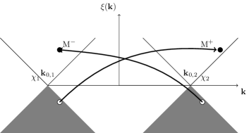
Figure 1: Low energy region of two isotropic Weyl nodes located at $\mathbf{k}_{0,2}=-\mathbf{k}_{0,1}$ with chirality $\chi_{2}$ and $\chi_{1}$, respectively. At zero temperature the filled Fermi sea (grey) is half-filled.

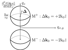
Figure 2: Region of nonzero scattering between two nodes at $\mathbf{k}_{0,2}=-\mathbf{k}_{0,1}={\text{k}}_{0}\hat{z}$. The cross-section as a function of momentum transfer $\mathbf{q}$ varies within spheres for $0\leq\lvert\bm{\Delta}\rvert\leq\hbar\omega/v_{\rm F}$.

II.1 Conditions for Lorentz invariance and its consequences

We will see below that Lorentz invariance leads to some special properties of the cross-section. First, there is a discontinuity of the cross-section at the surface of the spherical regions in momentum space where the cross-section is nonzero. Second, the variation of the cross-section as a function of momentum can be found using Lorentz transformations.

In contrast to a relativistic description of Weyl fermions, a condensed matter WSM manifestly breaksGrushin (2012) Lorentz invariance, because nodes are separated in momentum space and the $i^{th}$ Weyl node expanded to linear order in the momentum has the general anisotropic form

$$H_{0,i}(\mathbf{k}) = \sigma_{0}\mathbf{v}^{(i)}_{0}\cdot\mathbf{p}+\sigma_{l}v_{\rm F}\lambda^{(i)}_{l\,m}\text{p}_{m},$$ (2)

where $\sigma_{0}$ is the identity matrix and $\lambda_{lm}$ is a matrix of parameters (we use Einstein’s summation convention).

Now, we will focus on scattering between a pair of nodes that are related by either time-reversal or inversion symmetry. By this symmetry, we may assume the nodes are at $\mathbf{k}_{0,1}=-\mathbf{k}_{0}$ and $\mathbf{k}_{0,2}=\mathbf{k}_{0}$. By a linear transformation $\tilde{\mathbf{p}}=T\mathbf{p}$ (see Appendix A), the Hamiltonian of the $i^{\mathrm{th}}$ ($i=1,2$) low energy region can be turned into

$$H_{0,i}(\tilde{\mathbf{k}})=\sigma_{0}\mathbf{v}^{(i)}_{0}\cdot\tilde{\mathbf{p}}+\chi_{i}v_{\rm F}{\bm{\sigma}}\cdot\tilde{\mathbf{p}}\quad,\quad\tilde{\mathbf{p}}=\tilde{\mathbf{k}}-\tilde{\mathbf{k}}_{0,i}.$$ (3)

The type of symmetry connecting the Weyl nodes determines their relative chirality; for time-reversal and inversion symmetry, the chiralities are equal and negative of one another, respectively.

The transformation $T$ was chosen such that the second term in Eq. (2) transforms into the standard isotropic form of Eq. (3). If the term $\mathbf{v}^{(i)}_{0}$ is negligible, then the Hamiltonian is clearly isotropic and even has a relativistic symmetry. Importantly, because of the time-reversal or inversion symmetry, the transformation $T$ is the same for both nodes; i.e. the nodes have their principal axes aligned and are isotropic in a single coordinate system. This is crucial for our calculation of the cross-section; without it we would not be able to use Lorentz symmetry, and the contour of constant energy would not have the simple ellipsoidal shape that is found in Section V. As a consequence, the regions of nonzero scattering would not end sharply. In order to compare experimental results to this theory, it will be necessary to determine the transformation. We show in Section V.1 that it is easy to see the form of $T$ experimentally from a plot of the structure factor at fixed energy. The transformation must be chosen to have a determinant of $1$ to ensure that the density of states for exciting Weyl fermions does not change. Thus $v_{\rm F}$ will be the geometric mean of the three principal velocities of the original anisotropic dispersion.

The following conditions are the precise conditions under which Lorentz invariance can be assumed:

1. The nodes involved in the scattering are aligned (or nearly aligned) with the chemical potential. This requires careful doping for the materials discovered so far, but in a material where all the Weyl nodes are at the same energy, due to symmetry, it can be an automatic property of a compound with an even number of electrons per unit cell.

2. Scattering is between two nodes connected by either time-reversal or inversion symmetry.

3. The three components of $\mathbf{v}^{(i)}_{0}$ in Eq. (3) vanish. Although this condition would not usually be satisfied exactly, we will assume it to be, in order to be able to use Lorentz invariance. A small nonzero $\mathbf{v}_{0}$ does not change the predictions too much and, in fact, any type-I WSM $|\mathbf{v}_{0}|\leq v_{\rm F}$ is analytically tractable as will be discussed in Section V.1.

Under these conditions, the dynamics of the excitations of the material are entirely Lorentz invariant, but their interaction with neutrons is not. Thus the cross-section will not be Lorentz invariant, but it can be predicted using Lorentz symmetry. It turns out that the cross-section for a given initial and final neutron polarization is a certain component of a relativistic tensor (see Sec. IV); the tensor for any net momentum ${\tilde{\bm{\Delta}}}$ can be obtained by applying a Lorentz transformation to that in the rest frame. The cross-section is not Lorentz invariant for the same reason that the life-time of a particle depends on its velocity–namely, the lifetime is only one component of a 4-vector while the cross-section is one component of a 4-tensor. In the case of a moving particle, the Lorentz invariance can be proven by using a detector that is moving at the same speed as the particle, in which case the lifetime is the same as the rest-lifetime of the particle. In our case, the neutrons are not Lorentz invariant, so there is no way to accelerate the “detector”; we can only measure certain components of the scattering tensor in one reference frame.

II.2 Kinetic limitations on scattering between nodes at the same momentum

Consider now the case of intranode scattering, i.e., a transition within a single Weyl node. In this case, $\Delta\mathbf{k}_{0}=\bm{0}$. The conservation of energy and momentum give the same conditions on the transferred momentum and energy as above. However, in contrast to the case of distinct nodes where $\mathbf{q}_{i}-\mathbf{q}_{f}=\Delta\mathbf{k}_{0}-\bm{\Delta}$, there is no offset to the momentum, and this makes it much more difficult to see anything using neutron scattering. The same conclusion will apply to scattering between two Weyl nodes at the same point (e.g., in a Dirac material). First, it is clearly impossible to access the center of the spherical region described above, because $|\bm{\Delta}|=0$ implies that no momentum is transferred; therefore, the neutron’s momentum is unchanged, and so no energy is transferred either. For internode scattering, $|\bm{\Delta}|=0$ only implies that the transferred momentum is $\Delta\mathbf{k}_{0}$, and so the neutron’s energy can change, allowing it to create excitations in the material.

Second, there are no possible scattering events at all (with any transferred momentum) if the neutron has too small an energy. We initially assume an isotropic system, so that transformed and untransformed coordinates are the same, e.g. $\mathbf{q}_{i}=\tilde{\mathbf{q}}_{i},\mathbf{q}_{f}=\tilde{\mathbf{q}}_{f}$. Using $\hbar\omega\geq|{\tilde{\bm{\Delta}}}|v_{\rm F}$, the triangle inequality, $|{\tilde{\bm{\Delta}}}|\geq|\tilde{\mathbf{q}}_{i}|-|\tilde{\mathbf{q}}_{f}|$, and conservation of energy, $\hbar\omega=\frac{\hbar^{2}}{2m_{N}}(\mathbf{q}_{i}^{2}-\mathbf{q}_{f}^{2})$, we obtain $|\mathbf{q}_{i}|+|\mathbf{q}_{f}|\geq 2m_{\rm n}v_{\rm F}$, a restriction on the neutron momenta. Since the neutron loses energy and momentum, this relation constrains the velocity of the incident neutron $v_{\rm n}=|\mathbf{q}_{i}|/m_{\rm n}$ to

$$v_{\rm n}\geq v_{\rm F}.$$ (4)

In the more general case where the electron’s speed is direction-dependent, the neutron’s speed must exceed the maximum possible speed of the electron if one is to see the full region of scattering $|{\tilde{\bm{\Delta}}}|\leq\hbar\omega/v_{\rm F}$.

Hence, the Fermi velocity of the node determines a characteristic velocity scale for the neutronsGalilo (2013), implying that only neutrons moving faster than $v_{\rm F}$ can scatter on a single Weyl node. For example, ARPES measurements of tantalum phosphideXu et al. (2016) indicates a velocity of about $v_{\rm F}\approx 1.5\times 10^{5}\;{\rm m\,s^{-1}}$, which greatly exceeds the speedCarron (2007) of a thermal neutron $v_{\rm n}^{\rm thermal}=2\times 10^{3}\;{\rm m\,s^{-1}}$. In order to reach a speed of $10^{5}\;{\rm m\,s^{-1}}$ a neutron has to be rather hot, carrying an energy of the order of $10^{2}\;{\rm eV}$, which is far beyond what thermal neutron sources can offer and belongs within the resonance energy range. However, with the advent of ever-new WSMs, ones that allow observation of intranode scattering may be foundGuo et al. (2018). Hence, although we focus in this paper on scattering between separated Weyl nodes, Appendix D points out some differences that appear for intranode scattering.

III Operators for Neutron-Weyl Fermion Interaction

A Weyl fermion has two internal states, similar to a spin, but these do not necessarily correspond to spin–we call them pseudospin instead. The two states could, for example, be two orbitals of atoms with positive and negative orbital angular momentum $L_{z}$, or could differ in both spin and orbital degrees of freedom, or they could differ in some other way (they do not have to correspond to atomic orbitals of single atoms in fact). Because of this, the operator that interacts with the magnetic field of the neutron is not simply proportional to $\bm{\sigma}$. In this section, we will derive the most general form that this operator takes. It differs from the ordinary magnetic moment in an additional way–namely, it induces transitions between two different Weyl nodes.

III.1 Magnetic Moments of Weyl Fermions

The interactionBalcar and Lovesey (1989); Hirst (1997) of a neutron with the WSM is treated in the Born approximation, where the vector potential operator $\mathbf{A}(\mathbf{r})$ of the neutron’s magnetic moment interacts with the currents of the electronic system. If a full band structure is available, a direct way to calculate the structure factor would be to evaluate the matrix elements of the exact current operator (including spin and orbital parts) between the Bloch states. Near a Weyl point, one can focus on a few parameters from this calculation, which can be represented as an effective anomalous magnetic moment operator. See Appendix D for a discussion of why the interaction cannot be found by the minimal substitution in this case.

The basic idea is that the Weyl Hamiltonian in the vicinity of $\mathbf{k}_{0,i}$ can be developed just from information about the degenerate states exactly at these points. The Hamiltonian at a nearby point $H_{0,i}(\mathbf{k}_{0,i}+\mathbf{p})$ can be understood by treating $\mathbf{p}$ as a perturbation. We project it into the $2-$fold degenerate subspace $D_{i}=\{\lvert s;\mathbf{k}_{0,i}\rangle\}$ exactly at the nearby Weyl point, enumerated by arbitrary pseudospin label $s=\pm$. These are not necessarily different spin states; they are just any two degenerate states, and could differ in orbital structure instead of spin for example. For momenta $\mathbf{p}\neq 0$ away from the node, the projected Hamiltonian can be expanded to first order as $\mathbf{w}^{(i)}\cdot\mathbf{p}$ which removes the degeneracy, where $\mathbf{w}^{(i)}=\partial H_{0,i}(\mathbf{p}+\mathbf{k}_{0,i})/\partial\mathbf{p}|_{\mathbf{p}=\bm{0}}$ is a vector of $2\times 2$ matrices. Expanding in terms of Pauli matrices gives the effective low energy Weyl Hamiltonian Eq. (2), under the assumption that the nodes are aligned at the chemical potential. Note that the states $|s,\mathbf{k}_{0i}\rangle$ are not eigenstates at a nonzero $\mathbf{p}$; the energy eigenstates take the form $\sum_{s}c_{s}(\mathbf{p})|s;\mathbf{k}_{0i}\rangle$ where the $c_{s}$’s form an eigenvector of Eq. (2).

As mentioned above, neutron scattering depends on the matrix elements of the electronic current operator. These matrix elements have a complicated dependence on the “kinetic momenta” $\mathbf{p}$ of the states involved. However, this dependence can be derived from a simple effective description. There is an effective operator, a simple $2\times 2$ matrix that describes the electronic current within the low-energy subspaces. This matrix has no momentum dependence (to a good accuracy). However, it is defined with respect to the basis $|s;\mathbf{k}_{0i}\rangle$ which are not energy eigenstates; the momentum-dependence of the matrix elements appears because these eigenstates depend on momentum as $\sum_{s}c_{s}(\mathbf{p})|s;\mathbf{k}_{0,i}\rangle$.

For an $\text{M}^{+}$ transition, we need only the current’s overlaps between states of the degenerate subspaces $D_{1}$ and $D_{2}$. The current $\mathbf{J}$ forms a vector $\bm{\mathcal{J}}(2\mathbf{k}_{0})$ of $2\times 2$ matrices. The dependence on $\mathbf{p}$ can be neglected since the basis states are constant within the first order approximation aside from multiplication by $e^{i\mathbf{p}\cdot\mathbf{r}}$ to change the crystal momentum. (The basis states are nearly constant by the perturbation theory approach discussed above; the eigenstates vary strongly because $\mathbf{p}$ acts as a perturbation to a degenerate Hamiltonian). Within the effective Weyl fermion description, $\bm{\mathcal{J}}(2\mathbf{k}_{0})$ is the $1^{\mathrm{st}}$ quantized operator corresponding to the current; it has the same matrix elements for corresponding states in the effective and more realistic descriptions. Conservation of momentum gives

$$\langle s;\mathbf{k}_{0,2}+\mathbf{p}_{2}\rvert\mathbf{J}(\mathbf{q})\lvert\mathbf{k}_{0,1}+\mathbf{p}_{1};s^{\prime}\rangle={\delta}^{3}(\mathbf{q}-2\mathbf{k}_{0}+\bm{\Delta})\bm{\mathcal{J}}(2\mathbf{k}_{0})_{ss^{\prime}},$$ (5)

without any dependence of the matrix elements on ${\tilde{\bm{\Delta}}}$, which is valid for $|{\tilde{\bm{\Delta}}}|\ll|2\mathbf{k}_{0}|$ as is considered in this article. The electron-neutron coupling can now be reduced to

$$H_{\mathbf{A}}=-\int_{V}\textup{d}\mathbf{r}\,\mathbf{J}_{eff}(\mathbf{r})\cdot\mathbf{A}(\mathbf{r}-\mathbf{r}_{n})$$ (6)

where the Weyl-fermion current is given by

$$\mathbf{J}_{eff}(\mathbf{r},t)=\Psi_{2}^{\dagger}(\mathbf{r},t)\bm{\mathcal{J}}(2\mathbf{k}_{0})\Psi_{1}(\mathbf{r},t)+h.c.$$ (7)

and $\mathbf{A}(\mathbf{r}-\mathbf{r}_{\rm n})$ is the vector potential of a neutron at $\mathbf{r}_{\rm n}$.

This current can be interpreted as a magnetic moment. We first need a crucial fact that can be obtained by using conservation of charge $\partial\rho/\partial t+\bm{\nabla}\cdot\bm{\mathcal{J}}=0$ and Heisenberg’s equation of motion $\partial\rho/\partial t=(i/\hbar)\left[H,\rho\right]$ for the local electronic particle density operator. One finds that $2\mathbf{k}_{0}\cdot\bm{\mathcal{J}}(2\mathbf{k}_{0})=0$ since the matrix elements of $[H,\rho]$ are 0 between degenerate states. Hence the transition current density is purely transverse with respect to $2\mathbf{k}_{0}$ and can therefore be expressed as $\bm{\mathcal{J}}(2\mathbf{k}_{0})=-i2\mathbf{k}_{0}/\hbar\times\bm{\mathcal{M}}(2\mathbf{k}_{0})$. This operator has the interpretation of a magnetization operator. Substituting for $\bm{\mathcal{J}}$ in Eq. (7) in terms of $\bm{\mathcal{M}}$ and replacing $i2\mathbf{k}_{0}/\hbar$ by the gradient (which is valid for momenta near the nodes), we find $\mathbf{J}=\mathrm{curl}\ \mathbf{M}$ where

$$\mathbf{M}(\mathbf{r},t)=\Psi_{1}^{\dagger}(\mathbf{r},t)\bm{\mathcal{M}}^{\dagger}\Psi_{2}(\mathbf{r},t)+\Psi_{2}^{\dagger}(\mathbf{r},t)\bm{\mathcal{M}}\Psi_{1}(\mathbf{r},t).$$ (8)

This allows one to express the interaction between the neutron and the electrons, Eq. (6), as the standard form for the energy of a dipole in a magnetic field:

$$H_{\mathbf{B}}=-\int_{V}\textup{d}\mathbf{r}\,\mathbf{M}(\mathbf{r})\cdot\mathbf{B}(\mathbf{r}-\mathbf{r}_{n}).$$ (9)

Furthermore, the magnetization $\bm{\mathcal{M}}$, being a $2\times 2$ matrix, can be expanded as:

$$\bm{\mathcal{M}}=\mu_{\rm B}\sigma_{\mu}\mathbf{F}^{\mu}\quad,\quad\mu=0,1,2,3.$$ (10)

Defining the $j^{th}$ component of $\mathbf{F}^{\mu}\in\mathds{C}^{3}$ to be $\mathbf{F}^{\mu}$, a $4\times 3$ matrix which describes the coupling between the “magnetic” degree of freedom $j$ and the “pseudospin” degree of freedom $\mu$. Since these indices transform differently (one with spatial rotations and one with redefinition of the pseudospin basis), $\text{F}^{\mu}_{\hskip 4.26773ptj}$ is not a geometrical object. It is merely a collection of complex coupling coefficients which relate the magnetic moment to the spin, similar to the factor $\frac{g}{2}$ for an electron spin-$\frac{1}{2}$ magnetic moment $(g/2)\mu_{\rm B}{\bm{\sigma}}$ which Eq. (10) is a generalization of. Roughly, $\mathbf{F}^{\mu}$ can be interpreted as the “anomalous” components of a “Weyl magnetic moment”. However, it is not completely right to use this analogy. The reason is that the interaction involves a transition between states of two different nodes. Hence, the presence of the “anomalous magnetic moment” coupling $\mathbf{F}^{\mu}$ is a quantum effect from the bands, which acts like a force on the pseudospin.

The parameters $\mathbf{F}^{\mu}$ can be determined numerically if one has developed a realistic band structure model. Evaluating the current operator (including the currents associated with the spin) between the pair of degenerate wavefunctions gives a $2\times 2$ matrix from which one can obtain the $\mathbf{F}$’s. With respect to $\mathbf{k}_{0}$ these can be divided into longitudinal and transverse parts $\mathbf{F}^{\mu}=\mathbf{F}^{\mu}_{\parallel}+\mathbf{F}^{\mu}_{\perp}$. We have the freedom to set $\mathbf{F}^{\mu}_{\parallel}=\bm{0}$ and by Eq. (10) and the relation between $\bm{\mathcal{M}}$ and $\bm{\mathcal{J}}$, $\mathbf{F}_{\perp}$ can be found in two stages as:

$$\mathbf{F}^{\mu}_{\top} = \widehat{\mathbf{k}}_{0}\times\mathbf{F}^{\mu}=\frac{i\hbar}{2\lvert 2\mathbf{k}_{0}\rvert\mu_{\rm B}}\text{Tr}\left[\bm{\mathcal{J}}(2\mathbf{k}_{0})\sigma^{\mu}\right],$$ (11a)

$$\mathbf{F}^{\mu}_{\perp} = \mathbf{F}^{\mu}_{\top}\times\widehat{\mathbf{k}}_{0}.$$ (11b)

Contrary to conventional purely magnetic scattering, the coupling Eq. (11) is determined by sixteen real numbers without invoking constraints from symmetry. These contain information from bands solely, so without a specific band model these are unknown. Thus the coupling is structurally much more complicated than the bare coupling of neutrons with matter, which is just a single number with magnitude $g/2=1$. That is, $\mathbf{F}_{\perp}^{0}\neq\bm{0}$ generally and $\mathbf{F}_{\perp}^{i}\cdot\hat{j}\neq{\delta}_{ij}$ always, (by the constraint $2\mathbf{k}_{0}\cdot\mathbf{F}_{\perp}^{i}=0$), and can even be very asymmetric with either a larger or smaller value than the bare coupling. Furthermore, $\mathbf{F}^{\mu}_{\perp}$ may become divergent upon approaching $|2\mathbf{k}_{0}|\to 0$ a topological phase transition. An example of these features is illustrated in Section III.2 for a toy model.

III.2 Example: minimal $4$-band toy model of inversion invariant WSM

Analogous to Ref. Burkov et al., 2011; *Burkov2011b, a minimal time-reversal breaking and inversion invariant WSM can be obtained by starting with a material that is tuned to the transition between a topological and normal insulator and introducing magnetic impurities. In a time-reversal symmetric material that is tuned to the transition point, the gap is closed producing 3D Dirac points, which we suppose to be at momentum 0. The Dirac points are described by a Hamiltonian $H_{3\,\rm{D}}=v_{\rm D}\mathbf{k}\cdot{\bm{\sigma}}\tau^{z}$. These may be regarded as two Weyl nodes, labelled by $\tau^{z}=\pm 1$, and they have opposite chiralities, also given by $\tau_{z}$. The $\bm{\sigma}$s correspond to the spin of the state, while $\tau$ labels different bands. As one moves away from the topological transition, a hybridization term appears $H_{\delta}=\delta\sigma^{0}\tau^{x}$ that couples the nodes with strength $\delta$ and produces a gap. Returning to the transition point and introducing magnetic impurities $H_{\rm Z}=-m\sigma^{z}\tau^{0}$ that are assumed to order ferromagnetically along the z-direction and interact equally with both orbitals breaks time-reversal symmetry and separates the nodes in momentum space. If the hybridization term is present as well and not too large then it will not open a gap and the Weyl points will remain stable as long as $m>|\delta|$ assuming that $m>0$. This yields a basic minimal $4$-band toy model whose Hamiltonian $H^{0}_{4}=H_{3\,\rm D}+H_{\delta}+H_{\rm Z}$ has nodes at $\mathbf{k}_{0,2}=-\mathbf{k}_{0,1}={\text{k}}_{0}\hat{z}$, where $v_{\rm D}{\text{k}}_{0}=\sqrt{m^{2}-\delta^{2}}$, and its energy spectrum is plotted in Fig. 3.

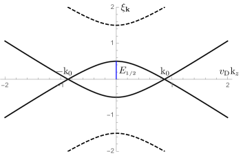
Figure 3: Energy spectrum of $4$-band model for $|\delta|/m=0.5$. The half-energy gap (blue line) $E_{\scriptscriptstyle 1/2}=m-|{\delta}|$ is indicated.

Each node $i=1,2$ has a degenerate subspace $D_{i}=\left\{\lvert s;\mathbf{k}_{0,i}\rangle\right\}$ enumerated by pseudospin $s=\pm$. The Hamiltonian is inversion symmetric, i.e. $PH^{0}_{4}(\mathbf{k})P^{-1}=H^{0}_{4}(-\mathbf{k})$, where inversion is $P=\sigma^{0}\tau^{x}$. As explained in Appendix A and B, in order to be sure that the effective Hamiltonian can be transformed into an isotropic form, the inversion symmetry must act as the identity–this is true within the space of degenerate states since $P\lvert s,\mathbf{k}_{1}\rangle=\lvert s,\mathbf{k}_{2}\rangle$. As expected the effective low energy Hamiltonians at the two Weyl points have the form of Eq. (2) with $\lambda^{(1)}=-\lambda^{(2)}=diag(+1,+1,-\sqrt{1-(\delta/m)^{2}})$, and $\mathbf{v}_{0}^{(i)}=\bm{0}$.

As we consider only scattering within the low energy sector of the nodes, the coupling Eq. (10) is determined by evaluating the matrix elements of the current exactly at the Weyl node positions, i.e. evaluating the left-hand side of Eq. (5) for the eigenfunctions of our model with $\mathbf{p}_{1}=\mathbf{p}_{2}=\bm{0}$, and comparing to the right-hand side evaluated using the effective description, Eq. (10). Note that in the effective model, the spin operators $\sigma^{i}$ are redefined to act on the two-dimensional subspace, e.g., $\sigma^{z}|s;\mathbf{k}_{0,i}\rangle=s|s;\mathbf{k}_{0,i}\rangle$, whereas the eigenstates are not eigenfunctions of the original $\sigma_{z}$. The $\mathbf{F}^{\mu}$ can then be solved for [giving Eq. (11)]. The current operator in this model is $\bm{\mathcal{J}}=ev_{\rm D}{\bm{\sigma}}\tau_{z}$; this is obtained by introducing a coupling to the vector potential into $H^{0}_{4}$ by a minimal substitution (see Appendix D for justification) and then comparing the term linear in $\mathbf{A}$ with Eq. (7). Consequently $\mathbf{F}_{\perp}^{\mu}$ has nonzero components $\text{F}^{x}_{\perp,x}$ and $\text{F}^{y}_{\perp,y}$, which both have the same magnitude,

$$\text{F}^{\perp}_{x\,x}=\frac{ev_{\rm D}}{\mu_{\rm B}}\frac{\delta}{m}\frac{\hbar}{\lvert 2\mathbf{k}_{0}\rvert}=\pm\frac{m_{\rm e}v_{\rm D}^{2}}{v_{\rm D}{\text{k}}_{0}}\frac{(v_{\rm D}{\text{k}}_{0})^{2}-E_{\scriptscriptstyle 1/2}^{2}}{(v_{\rm D}{\text{k}}_{0})^{2}+E_{\scriptscriptstyle 1/2}^{2}},$$ (12)

where $E_{\scriptscriptstyle 1/2}=m-|{\delta}|\leq v_{\rm D}{\text{k}}_{0}$ is the half-energy gap at $\mathbf{k}=\bm{0}$ indicated in Fig. 3. The second expression is written in terms of parameters of the bands’ dispersion; the sign just depends on the sign of $\delta$ which cannot be seen from the dispersion.

For example, for a Fermi velocity of order $v_{\rm D}=c/300$, the magnetic moment per Bohr magneton for the internode coupling, i.e. its $g/2$-factor, is plotted in Fig. 4 as a function of node position and half-energy gap. Hence the coupling of a neutron to nodes is comparable to, smaller or even much larger than that of the electron and may diverge upon approaching the topological phase transition. The cross-section will be estimated in the Section V.1. The above features hold, at least for this toy model which does not represent a realistic model. However, these features could be more generic in nature and hence present in real WSMs, but this question is left unanswered here. Alternatively some Weyl materials will be found that can actually be described as topological insulators with magnetic impurities.

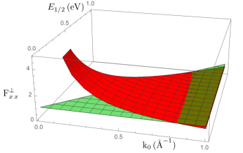
Figure 4: Coupling of neutron to Weyl fermions. The coupling, Eq. (12), for $v_{\rm D}=c/300$ is plotted (red) as a function of node position ${\text{k}}_{0}$ and half-energy gap $E_{\scriptscriptstyle 1/2}$ of spectrum in Fig. 3. The bare coupling of neutron to electrons, i.e. $g/2=1$, is the (green) plane.

IV Inelastic cross-Section and formalism

We will now present the formulae for scattering cross-sections. These results apply if the scattering is between two nodes that are related either by inversion or time reversal symmetry and that are aligned at (or near) the chemical potential. Furthermore, we need to assume that the three parameters $\mathbf{v}_{0}$ of Eq. (3) are negligible. These conditions allow the results to be obtained and interpreted in a relativistic way, as discussed above.

We will give the cross-section in detail, for arbitrary initial and final neutron polarization and arbitrary momentum and energy transfer. To be more precise, consider incident neutrons of a given momentum $\mathbf{q}_{i}$ and spin state represented by a spinor $|\tau_{i}\rangle$. Suppose a detector filters the neutrons according to their final momentum and spin eigenvalue $\pm 1/2$ along a specific direction and counts only the neutrons with eigenvalue $+1/2$, described by the state $|\tau_{f}\rangle$, say. Then the counting rate is proportional to the rate of transitions from the initial neutron state $\lvert i_{\rm n}\rangle=\lvert\mathbf{q}_{i};\tau_{i}\rangle$ via interactions with the WSM, defined by the Hamiltonian $H_{0,1}+H_{0,2}$, to the final state $\lvert f_{\rm n}\rangle=\lvert\mathbf{q}_{f};\tau_{f}\rangle$. The WSM begins in the ground state, $\lvert i_{\rm w}\rangle$, and ends in $\lvert f_{\rm w}\rangle$ upon absorbing neutron momentum $\mathbf{q}=\mathbf{q}_{i}-\mathbf{q}_{f}$ and energy $\hbar\omega$. The total differential cross-section is then

$$\frac{\text{d}^{2}\sigma(\mathbf{q},\omega)}{\text{d}\Omega\text{d}E_{f}}\bigg{|}_{\tau_{i}}^{\tau_{f}}\approx\frac{\text{q}_{f}}{\text{q}_{i}}\left(\frac{m_{\rm n}}{2\pi\hbar^{2}}\right)^{2}\frac{\mu_{0}^{2}}{2\pi\hbar}\sum_{l,m=1}^{3}\,\mu_{\perp,l}^{if}\mu_{\perp,m}^{fi}S_{l\,m}(\mathbf{q},\omega),$$ (13)

where the matrix element of the perpendicular component (with respect to the internode direction) of neutron magnetic moment is $\bm{\mu}^{fi}_{\perp}=\langle\tau_{f}\rvert\bm{\mu}_{\perp}\lvert\tau_{i}\rangle$.

The dynamic structure factor $S_{l\,m}(\mathbf{q},\omega)$ is the frequency and momentum Fourier transform of the scattering function $S_{l\,m}(\mathbf{r},t)$, which can be decomposed into $S_{l\,m}(\mathbf{r},t)=S^{(-)}_{l\,m}(\mathbf{r},t)+S^{(+)}_{l\,m}(\mathbf{r},t)$ (the contributions of the two processes $\text{M}^{\pm}$ defined in Fig. 2), since we can ignore intranode scattering. For the $\text{M}^{+}$ process

$$S^{(+)}_{i\,j}(\mathbf{r},t)\equiv V\left<\text{M}^{(-)}_{i}(\mathbf{r},t)\,\text{M}^{(+)}_{j}(\mathbf{0},0)\right>_{0},$$

which expresses the fact that it is a van Hove type correlation function of magnetization operators Eq. (8). The structure factor of an $\text{M}^{-}$ transition follows trivially from that of an $\text{M}^{+}$ transition simply by interchanging Weyl node labels $1\leftrightarrow 2$.

The structure factor $S_{l\,m}(\mathbf{q},\omega)$ considered as a function of neutron momentum transfer $\mathbf{q}=2\mathbf{k}_{0}-\bm{\Delta}$, will be concentrated in small spheres centered at $2\mathbf{k}_{0}$ as illustrated in Fig. 2. To focus on this region, it is convenient to describe the cross-section in a coordinate system of ${\tilde{\bm{\Delta}}}$.

The previous expression can be written as

$$S^{(+)}_{ij}(\mathbf{r},t)=\mu_{\rm B}^{2}\text{F}^{\mu,*}_{i}\text{F}^{\nu}_{j}\sigma^{(+)}_{\mu\,\nu}(\mathbf{r},t),$$ (14)

where the intermediate scattering function

$$\sigma^{(+)}_{\mu\,\nu}(\mathbf{r},t)=\langle\Psi_{1}^{\dagger}(\mathbf{r},t)\sigma_{\mu}\Psi_{2}(\mathbf{r},t)\Psi_{2}^{\dagger}(\mathbf{0},0)\sigma_{\nu}\Psi_{1}(\mathbf{0},0)\rangle_{0}V,$$ (15)

is a particle-hole correlator of the relativistic Weyl fermions. It can be related to the absorptive part of the generalized susceptibility $\chi^{(+)}_{\mu\,\nu}$ by the fluctuation-dissipation theorem. For conventional neutron scattering, the neutrons interact mainly with the spin degrees of freedom and hence $\sigma_{\mu\nu}^{(+)}(\mathbf{q},\omega)/2\hbar$ describes the spin susceptibility. In this case, the states of the Weyl fermions are pseudospin states, so $\sigma$ does not correspond to the spin. Instead, $\sigma_{\mu\nu}^{(+)}(\mathbf{q},\omega)/2\hbar$ describes the full magnetic susceptibility including both orbital and spin contributions to the magnetic moments, since we determined the magnetization operator in a way that includes all these contributions.

The susceptibility can be calculated by integrating over all possible Weyl particle-hole pairs. At zero temperature we exploit Lorentz invariance to evaluate this analytically (see Appendix C). When the nodes are related by time-reversal symmetry, they have the same chirality, say $\chi_{i}=\chi_{f}=\chi$. The susceptibility for the scattering process is

$$\chi^{\prime\prime\mu\,\nu}_{(+)}(\mathbf{q},\omega)=\sigma^{\mu\,\nu}_{(+)}(\mathbf{q},\omega)/2\hbar.$$ (16)

For time-reversal symmetric nodes it is a Lorentz invariant rank-$2$ tensor with components:

$$a^{-1}\chi^{\prime\prime 0\,0}_{(+)}(\mathbf{q},\omega) = \lvert{\tilde{\bm{\Delta}}}\rvert^{2}$$ (17a)

$$a^{-1}\chi^{\prime\prime 0\,i}_{(+)}(\mathbf{q},\omega) = a^{-1}\chi^{\prime\prime i\,0}_{(+)}(\mathbf{q},\omega)=\chi(\hbar\omega/v_{\rm F})\tilde{\Delta}_{i}$$ (17b)

$$a^{-1}\chi^{\prime\prime i\,j}_{(+)}(\mathbf{q},\omega) = \tilde{\Delta}_{i}\tilde{\Delta}_{j}+{\delta}_{i\,j}[\left(\hbar\omega/v_{\rm F}\right)^{2}-\lvert{\tilde{\bm{\Delta}}}\rvert^{2}]\hskip 7.11317pt$$ (17c)

with

$$a=\frac{\pi^{2}}{3}\frac{V}{v_{\rm F}(2\pi\hbar)^{3}}.$$ (18)

When the symmetry between the nodes is inversion, they have opposite chiralities, which we take to be $\chi_{i}=-\chi_{f}=\chi$. In this case Eq. (16) breaks up into different tensors:

$$a^{-1}\chi^{\prime\prime 0\,0}_{(+)}(\mathbf{q},\omega) = (3/2)[\left(\hbar\omega/v_{\rm F}\right)^{2}-|{\tilde{\bm{\Delta}}}|^{2}]$$ (19a)

$$a^{-1}\chi^{\prime\prime 0\,i}_{(+)}(\mathbf{q},\omega) = a^{-1}\chi^{\prime\prime i\,0}_{(+)}(\mathbf{q},\omega)=0$$ (19b)

$$a^{-1}\chi^{\prime\prime i\,j}_{(+)}(\mathbf{q},\omega) = {\delta}_{i\,j}[\left(\hbar\omega/v_{\rm F}\right)^{2}+|{\tilde{\bm{\Delta}}}|^{2}]/2-\tilde{\Delta}_{i}\tilde{\Delta}_{j}$$ (19c)

$$+ \chi\,i\,\epsilon_{i\,j\,k}\left(\hbar\omega/v_{\rm F}\right)\tilde{\Delta}_{k}$$

Clearly, $\chi^{\prime\prime 0\,0}_{(+)}$ is a Lorentz scalar. The other tensor does not look Lorentz covariant since it has only spatial indices, but it actually is a usual type of tensor, see Appendix C.

Now, by combining Eq. (13) and (14) with either the time-reversal or inversion-symmetric susceptibility, Eq. (17) or (19), we get the general expressions for scattering with both a polarized beam and a polarized detector. All these results are in the isotropic coordinate system obtained from the physical one by applying the transformation ${\tilde{\bm{\Delta}}}=T\mathbf{\Delta}$. Section V.1 explains how to find the appropriate transformation $T$ experimentally.

In realistic neutron scattering experiments, the initial neutron beam of $N$ neutrons has an average polarization vector $\mathbf{P}$, which can be described by a density matrix $\bm{\rho}=\left(\tau_{0}+\mathbf{P}\cdot\bm{\tau}\right)/2$, where $\bm{\tau}$ is a vector of Pauli matrices and $\tau_{0}$ the identity matrix in neutron spin basis. The inelastic cross-section Eq. (13) of the scattered beam measured by an unpolarized detector is given byLovesey (1984); Hirst (1997)

$$\frac{\text{d}^{2}\sigma^{(+)}(\mathbf{q},\omega;\mathbf{P})}{\text{d}\Omega\text{d}E_{f}} = \frac{\text{q}_{f}}{\text{q}_{i}}\left(\frac{gr_{0}}{4}\right)^{2}\left[\Sigma^{(+)}(\mathbf{q},\omega)+\mathbf{P}\cdot\bm{\Sigma}^{\prime(+)}(\mathbf{q},\omega)\right]$$

where $$\Sigma^{(+)} \bm{\Sigma^{\prime}}{(+)}$$ and can be found using Eq. (14),

$$\Sigma^{(+)}(\mathbf{q},\omega) \equiv \hskip 5.83286pt\left<\mathbf{M}^{(-)}_{\perp}(-\mathbf{q},-\omega)\hskip 2.13387pt\cdot\hskip 2.13387pt\mathbf{M}^{(+)}_{\perp}(\mathbf{q},\omega)\right>/2\pi\hbar\mu_{\rm B}^{2},$$ (20a)

$$= \hskip 3.55658pt\mathbf{F}^{\mu,*}_{\perp}\cdot\mathbf{F}^{\nu}_{\perp}\chi^{(+)}_{\mu\,\nu}(\mathbf{q},\omega)/\pi,$$

$$\bm{\Sigma}^{\prime(+)}(\mathbf{q},\omega) \equiv i\left<\mathbf{M}^{(-)}_{\perp}(-\mathbf{q},-\omega)\times\mathbf{M}^{(+)}_{\perp}(\mathbf{q},\omega)\right>/2\pi\hbar\mu_{\rm B}^{2},$$ (20b)

$$= i\mathbf{F}^{\mu,*}_{\perp}\times\mathbf{F}^{\nu}_{\perp}\chi^{(+)}_{\mu\,\nu}(\mathbf{q},\omega)/\pi.$$

The coefficients $\mathbf{F}^{\mu,*}_{\perp}\cdot\mathbf{F}^{\nu}_{\perp}$ and $\mathbf{F}^{\mu,*}_{\perp}\times\mathbf{F}^{\nu}_{\perp}$ select which components of $\chi_{\mu\nu}$ are measured by neutron scattering. The $(\mu,\nu)=(0,0)$ component give rise to no angular ${\tilde{\bm{\Delta}}}$ dependence. However, the remaining hermitian ($i,j=1,2,3$) parts do and can be written in their spectral decompositions

$$\mathbf{F}^{i,*}_{\perp}\cdot\mathbf{F}^{j}_{\perp} = \sum_{l=1}^{2}\,\alpha_{l}\,\widehat{\mathbf{a}}^{l}_{j}\,\widehat{\mathbf{a}}^{l*}_{i},$$ (21a)

$$\mathbf{F}^{i,*}_{\perp}\times\mathbf{F}^{j}_{\perp} = -i\widehat{\mathbf{k}}_{0}\sum_{l=1}^{2}\,\beta_{l}\,\widehat{\mathbf{b}}^{l}_{i}\,\widehat{\mathbf{b}}^{l*}_{j},$$ (21b)

where $\alpha_{l}(\beta_{l})$ and $\widehat{\mathbf{a}}^{l}(\widehat{\mathbf{b}}^{l})$ are the $l^{th}$ eigenvalue and normalized eigenvector of matrix $\mathbf{F}^{i,*}_{\perp}\cdot\mathbf{F}^{j}_{\perp}$ ($i\widehat{\mathbf{k}}_{0}\cdot\mathbf{F}^{i,*}_{\top}\times\mathbf{F}^{j}_{\top}$). To prove these, we used the fact that $\mathbf{F}^{i}_{\perp}\cdot\widehat{\mathbf{k}}_{0}=0$ for each $i$, hence $\mathrm{det}[\mathbf{F}^{i}\cdot\hat{j}]=0$ and therefore Eq. (21) will have a zero eigenvalue.

V Experimental predictions and interpretation

The results of the last section have several conceptually and experimentally interesting special cases. Although there are many parameters describing the coupling of neutrons to Weyl fermions, there are some universal predictions contained in these formulae. In addition, one can observe spin-momentum locking even without using polarized neutron beams or measuring the polarization of the scattered neutrons. Furthermore, with a polarized measurement, it is possible to determine the chiralities of the Weyl fermions in the inversion-symmetric case, without knowing the coupling parameters.

The scattering process is distinguished by whether the symmetry relation between the two nodes involved is inversion or time-reversal. While the density of states is the same for either type of symmetry, the cross-sections differ, for two reasons. First, the chiralities are different in the two cases and hence the relativistic susceptibilities have different forms, see Eq. (17) and (19). Second, the symmetry constraints on the coupling between neutrons and Weyl nodes are different for time-reversal and inversion symmetry. Appendix B shows that

$$\mathbf{F}^{0}=\bm{0}\quad,\quad\mathbf{F}^{j}\in\mathds{C}^{3}\text{ with }j=1,2,3$$ (22)

for time-reversal symmetric nodes, whereas

$$\mathbf{F}^{\mu}\in\mathds{R}^{3}\text{ with }\mu=0,1,2,3$$ (23)

for inversion symmetric nodes. As the predictions will be different for time-reversal and inversion symmetric nodes, they will be discussed separately.

V.1 Measurement of dispersion, principal axes and velocities

The rate of neutron scattering depends on what final electron-hole states can be produced in the material. This is determined by the number of final states and the matrix element for creating the particle-hole pair. We will begin by describing the possible final states and estimating the density of states (DOS). Understanding the density of states will help to understand a few features of the scattering cross-section, and in particular will show how one can measure the linearity of the Weyl fermion dispersion and determine its principal axes and the velocities along them.

The DOS is defined as an integral over all internal states that conserve energy and momentum:

$$D({\tilde{\bm{\Delta}}},\omega)=\iint\frac{d^{3}\tilde{\mathbf{p}}_{i}d^{3}\tilde{\mathbf{p}}_{f}}{(2\pi\hbar)^{3}}\delta^{3}(\tilde{\mathbf{p}}+{\tilde{\bm{\Delta}}})\delta(\hbar\omega-\Delta\xi^{\rm w}).$$ (24)

The set of allowed momenta have a simple geometric description, see Fig. 5. Plot a point at the origin and a point displaced from this by ${\tilde{\bm{\Delta}}}$. If the initial electron momentum is represented by a point $P$ displaced from the origin by $\tilde{\mathbf{p}}_{i}$, then the final momentum is the vector from ${\tilde{\bm{\Delta}}}$ to $P$, according to conservation of momentum. The change in energy is $v_{\rm F}(|\tilde{\mathbf{p}}_{f}|+|\tilde{\mathbf{p}}_{i}|)$, so conservation of energy forces $P$ to lie on a prolate ellipsoid with foci at $\mathbf{0}$ and ${\tilde{\bm{\Delta}}}$. When $|{\tilde{\bm{\Delta}}}|=0$, the ellipsoid turns into a sphere; when $|{\tilde{\bm{\Delta}}}|=\hbar\omega/v_{\rm F}$, the ellipsoid degenerates into a line segment connecting the two foci; and for any smaller ratio of $\hbar\omega/v_{\rm F}$ to $|{\tilde{\bm{\Delta}}}|$ there are no final states compatible with conservation laws. Hence, the region of nonzero DOS is defined by $|{\tilde{\bm{\Delta}}}|\leq\hbar\omega/v_{\rm F}$ and within this region the density of states is found to be

$$D({\tilde{\bm{\Delta}}},\omega)=\frac{\pi}{2v_{\rm F}(2\pi\hbar)^{3}}[\left(\hbar\omega/v_{\rm F}\right)^{2}-(1/3)|{\tilde{\bm{\Delta}}}|^{2}]$$ (25)

We remark, first of all, that this shows that the scattering cross-section scales as the square of the transferred energy like the DOS for a single node. This makes the scattering cross-section small at low energies. This can be problematic, since experiments must be restricted to energies small enough that the Weyl Hamiltonian is correct. In particular, the momentum transfer can be at most of order $|\mathbf{k}_{0}|$ since beyond that distance from one Weyl point, the other Weyl Hamiltonian becomes a better approximation. Luckily, the small size of the cross-section at small energies can be compensated by the possibility that the coupling to the neutrons is larger than the usual $g$-factor of the electrons. To illustrate this, we employed a WSM toy model in Section IIIB. The factors F are enhanced and even diverge as the spacing between the Weyl nodes approaches zero, which can compensate for the small DOS. This is actually more general than this specific model. In Eq. (11), the current matrix element $\bm{\mathcal{J}}(2\mathbf{k}_{0})$ depends on two contributions to the currentBalcar and Lovesey (1989), orbital and spin current. The orbital Schrödinger current is proportional to the velocity, represented by the operator $\frac{\hbar}{m_{e}i}\bm{\nabla}_{\mathbf{R}}$ where $\mathbf{R}$ is the position of the electron, and hence the current at a specific point is $\mathbf{J}_{orbital}(\mathbf{r})=\frac{e\hbar}{2m_{e}i}\{\bm{\nabla}_{\mathbf{R}},\delta(\mathbf{r}-\mathbf{R})\}$. (Here $\{a,b\}$ represents the anticommutator of the two operators.) The spin current is described by an infinitesimal spinning sphere, which can be represented by the gradient of a delta-function, $\mathbf{J}_{spin}(\mathbf{r})=\frac{g\mu_{\text{B}}}{2}\bm{\sigma}\times\bm{\nabla}_{\mathbf{r}}\delta(\mathbf{r}-\mathbf{R})$. The matrix element of the spin current comes out to be the structure factor that usually determines neutron cross-sections: taking the Fourier transform causes the delta function to be replaced by $e^{-2i\mathbf{k}_{0}\cdot\mathbf{R}}$ and the gradient gives a factor of $2\mathbf{k}_{0}$ that cancels the factor in the denominator of Eq. (11). However, in the orbital current, the gradient acts on the electron position $\mathbf{R}$ rather than $\mathbf{r}$, hence this produces a factor of $1/d$ where $d$ is the length scale for variation of the phase of the electronic wave functions, which, if the imaginary parts of the wave-functions, due to spin-orbit coupling for example, are large, can be the same as the size of an atom. Thus, $\mathrm{F}_{x,x;\perp}$ is of order $1/k_{0}d$, so if accidentally the two Weyl points happen to be close to one another, the coupling is large. Even if the Weyl points are separated by an amount on the order of the Brillouin zone, $1/k_{0}d$ will be large if a unit cell contains many atoms. To get a real estimate one needs to know in detail the form of the wave functions; in particular, the wave-functions might have small imaginary parts, or the orbitals at the two Weyl points might be separated in space, and then F would be small because of the small overlap integral of the orbitals.

To give a concrete estimate of the unpolarized cross-section, Eq. (20a), we return to the 4-band model. For internode scattering it has magnitude

$$\frac{1}{V}\frac{\text{q}_{i}}{\text{q}_{f}}\frac{\text{d}^{2}\sigma^{(+)}(\mathbf{q},\omega)}{\text{d}\Omega\text{d}E_{f}} = \left(\frac{gr_{0}}{4}\right)^{2}\frac{\pi}{3}\frac{(\hbar\omega)^{2}}{(2\pi\hbar v_{\rm F})^{3}}\text{F}^{x}_{x,\perp}\text{F}^{x}_{x,\perp},\hskip 14.22636pt$$ (26)

$$\lesssim 5\cdot 10^{-2}\frac{v_{\rm F}}{c}\;\frac{\rm mb}{\rm meV\,\r{A}^{3}\,Sr}.$$ (27)

The expression Eq. (26) is a generally applicable expression with coupling given by Eq. (12), whereas Eq. (27) is an estimate for the 4-band model. We made the following substitutions. Since $\chi_{\mu\nu}$ was derived in the isotropic coordinate system, the factor of $v_{\rm F}$ is not the physical velocity. The physical Weyl nodes have three eigen-velocities; the two perpendicular to the internode direction are equal to $v_{\rm D}$ whereas that parallel is smaller, and $v_{\rm F}$ should be the geometric mean of all three. In the above, we conservatively took all three velocities to be identical, i.e., $v_{\rm D}=v_{\rm F}$. The intensity would be higher than Eq. (27) if one took account of the anisotropy. Further, the energy transfer $\hbar\omega$ has been expressed in terms of the displacement of the momenta of the excitations from the Weyl point. We have taken the value $\mathrm{k}_{0}$, which is the largest possible as explained above. Since the result scales as $\omega^{2}$, the cross-section decreases quickly for momenta below this optimistic value. Finally $\mathrm{F}_{x,x;\perp}^{2}$ is taken as $(m_{e}v_{\rm D}/\mathrm{k}_{0})^{2}$. Despite the fact that $\chi_{\mu\nu}$ is suppressed by a factor $(\hbar\omega)^{2}/v_{\rm F}^{3}\propto\mathrm{p}^{2}/v_{\rm F}$ from the DOS, the coupling squared, $\mathrm{F}_{x,x;\perp}^{2}$, partly cancels this suppression leaving the product to have an order $\lesssim v_{\rm F}$ resulting in Eq. (27). This implies that a higher node velocity leads to a higher intensity of the cross-section. For a typical Fermi velocity $v_{\rm F}=c/300$ Eq. (27) is $\lesssim 1.7\times 10^{-4}\;{\rm mb}/{\rm meV\,\r{A}^{3}\,sr}$. Now assuming a typical unit cell has volume $V=(5\rm\r{A})^{3}$, the intensity $\text{q}_{i}/\text{q}_{f}\times\text{d}^{2}\sigma^{(+)}(\mathbf{q},\omega)/\text{d}\Omega\text{d}E_{f}\lesssim 2\times 10^{-2}\;{\rm mb}/{\rm meV\,sr\,f.u.}$. As anticipated for a semimetal the intensity is low, but much higher than the early estimatesSilver (1984) of the neutron cross-section for one-electron metallic band structures, which were of order $10^{-4}-10^{-3}{\rm mb/meV\,sr}$. Our estimate for the $4$-band model is only of order $10^{-2}-1$ smaller than what has been observed in scattering off spin-$\frac{1}{2}$ particle-hole pairs Goremychkin et al. (2018); Vignolle et al. (2007); Walters et al. (2009); Fujita et al. (2012); Janoschek et al. (2015).

One other property of the Weyl scattering cross-section may also help it to be visible–namely at the maximum momentum transfer the DOS is still nonzero, and then there is a sharp jump down to zero. A sharp jump can be separated out when there is a smooth background, even if the background is large, by differentiating.

Let us understand why the DOS has a sharp jump. Imagine fixing the transferred momentum and lowering the energy. The set of final states is always a prolate ellipsoid with the same foci $\mathbf{0}$ and $\tilde{\bm{\Delta}}$, that eventually degenerates to a line segment at the minimum possible energy transfer. Because there is a whole line segment rather than a single final state, the DOS is larger than usual in this limit. To be more precise, let $\Delta\xi^{\rm w}(\tilde{\mathbf{p}}_{i})$ be the change in energy of the electron as a function of the initial momentum ($\tilde{\mathbf{p}}_{f}=\tilde{\mathbf{p}}_{i}-{\tilde{\bm{\Delta}}}$ since ${\tilde{\bm{\Delta}}}$ is fixed), $\Delta\xi^{\rm w}(\tilde{\mathbf{p}}_{i})=v_{\rm F}(|\tilde{\mathbf{p}}_{i}|+|\tilde{\mathbf{p}}_{i}-{\tilde{\bm{\Delta}}}|)$. The DOS of the particle-hole pair is given by $(2\pi\hbar)^{-3}\int d^{3}\tilde{\mathbf{p}}_{i}\,\delta(\Delta\xi^{\rm w}(\tilde{\mathbf{p}}_{i})-\hbar\omega)$, which is the same formula used to calculate the DOS of a single particle whose dispersion happens to be given by $\Delta\xi^{\rm w}(\tilde{\mathbf{p}_{i}})$. We will use this analogy to understand the behaviour of the particle-hole pair DOS at the surface of the spherical scattering region. Here its behaviour corresponds to a van Hove singularity. To see this, notice that the function $\Delta\xi^{\rm w}$ has a minimum value $\Delta\xi^{\rm w}_{min}=v_{F}|{\tilde{\bm{\Delta}}}|$. Increasing $|{\tilde{\bm{\Delta}}}|$ with a fixed $\omega$, beyond the surface of the scattering region, is equivalent to letting $\hbar\omega$ fall below this minimum value. Generically, in three-dimensions the DOS close to a minimum should have the van Hove dependence of $\sqrt{\hbar\omega-\Delta\xi^{\rm w}_{min}}$. This assumes that the minimum is at an isolated point. However, for the pair of Weyl excitations, there is a line which $\Delta\xi^{\rm w}$ is minimum on, the line connecting the foci of the ellipsoid. The DOS may be found by integrating over layers perpendicular to the line connecting foci. For example, if ${\tilde{\bm{\Delta}}}$ is parallel to the $z$-axis, $D(\omega)=\int\frac{\textup{d}\tilde{p}_{z}}{2\pi\hbar}D_{\perp}(\tilde{p}_{z})$ where $D_{\perp}$ is the DOS in one of these planes. For each fixed $\tilde{p}_{z}$, $D_{\perp}$ has the van Hove singularity one expects in two dimensions (this function is quadratic near its minimum except in the planes passing through the foci), that is, it should jump from 0 to a nonzero value. Since the minimal values of $\omega$ are equal for all planes between the foci, there is still a discontinuous jump after integrating over $\tilde{p}_{z}$ and thus also in $D(\omega)$.

If the transferred energy is fixed, the region of nonzero scattering is a sphere of radius $\hbar\omega/v_{\rm F}$. Thus, by measuring the radius of this sphere as a function of the transferred energy one may deduce the dispersion velocity of the Weyl fermions. Furthermore, the linear relationship between the radius of the sphere and the energy reflects the linear dispersion of the Weyl fermions. Now this region is spherical only because we began by rescaling all momenta to make the dispersion isotropic. In general, the dispersion of Weyl fermions is likely to be anisotropic; it has the form $\sqrt{\sum_{i\,j}(v^{2})_{i\,j}\mathbf{p}_{i}\mathbf{p}_{j}}$ where $v^{2}$ is a certain matrix. Indeed, when one diagonalizes Eq. (2), one finds that the energy of the excitation has this form, with $v^{2}=v_{\rm F}^{2}\lambda^{T}\lambda$. By the inversion or time-reversal symmetry, both Weyl particles have the same dispersion. One can then show that the region of allowed momentum and energy transfers is $\hbar\omega\geq v_{\rm F}\sqrt{\sum_{i\,j}(\lambda^{T}\lambda)_{i\,j}\mathbf{p}_{i}\mathbf{p}_{j}}$, which is an ellipsoid for each fixed $\omega$ rather than a sphere. It has the same shape as the equal-energy contours of a single particle. The directions and lengths of the principle axes give the eigenvectors and eigenvalues of $v^{2}$. Let $T$ be any linear transformation that distorts this ellipsoid to a sphere; then the dispersion becomes isotropic upon redefining $\tilde{\mathbf{p}}=T\mathbf{p}$. The Weyl equation then takes the form in Eq. (1). In this way, one can measure from the cross-section the principal axes, velocities of the dispersion as well as the transformation $T$ that will be important to be able to see the “universal” predictions of this theory below.

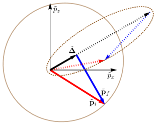
Figure 5: Contour of constant energy transfer $\hbar\omega$ for Weyl excitations produced in an scattering event: A prolate spherioid (brown line) in the $\tilde{p}_{x},\tilde{p}_{z}$-plane with symmetry axis (black arrow) along ${\tilde{\bm{\Delta}}}$ and foci at origin of initial $\tilde{\mathbf{p}}_{i}$ (red arrow) and final $\tilde{\mathbf{p}}_{f}$ (blue arrow) excitations for a given $|{\tilde{\bm{\Delta}}}|$. Full (dottted) lines are for $|{\tilde{\bm{\Delta}}}|=0.25\hbar\omega/v_{\rm F}$ ($|{\tilde{\bm{\Delta}}}|=0.95\hbar\omega/v_{\rm F}$).

The discontinuous jump is unique to the case where $\mathbf{v}^{(i)}_{0}=\bm{0}$ in Eq. (2). When the vector $\mathbf{v}^{(i)}_{0}$ is nonvanishing then its values at the two nodes are negative of one another by symmetry (either inversion or time reversal), i.e., $\mathbf{v}_{0}^{(1)}=-\mathbf{v}_{0}^{(2)}=\mathbf{v}_{0}$. By transforming the coordinates, one can still make $\lambda_{i\,j}^{(1)}=\pm\lambda_{i\,j}^{(2)}=\delta_{i\,j}$ and additionally make $\mathbf{v}_{0}$ parallel to any direction one prefers. One then sees that there is only one parameter in the Hamiltonian that is important: the ratio $|\mathbf{v}_{0}|/v_{\rm F}\equiv\alpha$, which for a type-I WSM takes valuesSoluyanov et al. (2015) $0\leq\alpha<1$. The parameter $\alpha$ upsets Lorentz invariance more seriously than the coupling parameters $\mathbf{F}^{\mu}$. It changes the kinematics, such that the constant energy contour is not an ellipsoid any longerBjerngaard et al. . It also appears in a nontrivial way in the structure factor Eq. (15). A specific effect is that the cross-section will not jump suddenly to zero at the edge (see Fig. 6 and 7); it vanishes continuously. If $\alpha$ is small, this jump happens in a layer of a thickness proportional to $\alpha$, so when $\alpha$ is very small, it seems to be a sharp jump. On the other hand, the spin-momentum locking could still be observed; it would still cause the cross-section to vary strongly as a function of the angle around the center of the region. The formula for the variation would not be so simple as that given here.

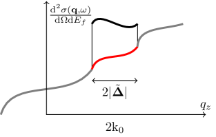
Figure 6: Sketch of cross-section including background scattering along $q_{z}$ in Fig. 2 for the $\text{M}^{+}$ process. The intensity jumps discontinuously at the boundary between the region describing internode scattering (black curve) and that which does not (gray curve), while there might be background scattering (red curve) in the region of interest.

V.2 Probing spin-momentum locking in a fully unpolarized experiment

We have previously just quoted the susceptibility. Now we turn to an intuitive explanation of it in terms of simple concepts of spin matrix elements and spin-momentum locking, thereby enabling us to understand how a fully unpolarized measurement can probe the spin-momentum locking of Weyl spinors, which at first seems like a contradiction. Appendix C gives a different interpretation of the results in terms of Lorentz transformations of spinors.

To guide our intuition, we will explain it here for the case of coupling strengths that most closely resemble conventional purely magnetic scattering, i.e. $\mathbf{F}^{0}=\bm{0}$ and $\text{F}_{i\,j}={\delta}_{i\,j}$. We will assume that the nodes are on the $z$-axis, $\mathbf{k}_{0,2}=-\mathbf{k}_{0,1}={\text{k}}_{0}\hat{z}$. Then the cross-section Eq. (20) becomes $\pi\Sigma^{(+)}(\mathbf{q},\omega)=\sum_{i=1}^{2}\chi^{\prime\prime(+)}_{i\,i}(\mathbf{q},\omega)$. This clearly highlights the fact, see Eq. (11), that neutrons couple only to components of the coupling vectors that are perpendicular to the internode direction. This has the desirable consequence that the cross-section will have angular ${\tilde{\bm{\Delta}}}$ dependence, which is a signature of probing spin-momentum locking of Weyl spinors.

A consequence of momentum conservation is that initial $\lvert i_{\rm w}\rangle=\lvert\widehat{\tilde{\mathbf{p}}}_{i};-\chi_{i}\rangle$ and final $\lvert f_{\rm w}\rangle=\lvert\widehat{\tilde{\mathbf{p}}}_{f};+\chi_{f}\rangle$ Weyl states are related by $\tilde{\mathbf{p}}_{f}=\tilde{\mathbf{p}}_{i}-{\tilde{\bm{\Delta}}}$, and energy conservation dictates that any pair $\tilde{\mathbf{p}}_{i}$ and $\tilde{\mathbf{p}}_{f}$ are restricted to the ellipsoid constant energy contour in Fig. 5. In the limit ${\tilde{\bm{\Delta}}}=\bm{0}$, the allowed initial and final states are pairs $\tilde{\mathbf{p}}_{f}=\tilde{\mathbf{p}}_{i}$ on a sphere of radius $\hbar\omega/2v_{\rm F}$, and the polarization vectors of the Weyl spinors are thus related by

$$\langle f_{\rm w}\rvert{\bm{\sigma}}\lvert f_{\rm w}\rangle = \mp\langle i_{\rm w}\rvert{\bm{\sigma}}\lvert i_{\rm w}\rangle\text{ for }\chi_{f}=\pm\chi_{i},$$ (28)

i.e. initial and final spinors are antiparallel (parallel) for same (opposite) chirality. (To understand this, remember that the initial state has a negative energy and the final state has a positive energy.) All these different spinors just contribute to the cross-section at a single point, so there is no signature that distinguishes between $\chi_{f}=\pm\chi_{i}$ apart from a constant factor of 2 (which cannot be measured anyway unless one knows the values of the $\mathrm{F}$’s).

For increasing $\lvert{\tilde{\bm{\Delta}}}\rvert$ the energy conserving contour takes a more extreme prolate spheroid form and the cross-section will have angular ${\tilde{\bm{\Delta}}}$ dependence because the Weyl state contributions depend on the direction of ${\tilde{\bm{\Delta}}}$.

In the extreme limit $|{\tilde{\bm{\Delta}}}|\approx\hbar\omega/v_{\rm F}$ the energy conserving contour becomes an extremely slim, elongated prolate spheroid, which degenerates to a line at maximum $|{\tilde{\bm{\Delta}}}|=\hbar\omega/v_{\rm F}$. The initial and final unit vectors along the momenta are therefore approximately $\widehat{\tilde{\mathbf{p}}}_{i}\approx\widehat{{\tilde{\bm{\Delta}}}}\approx-\widehat{\tilde{\mathbf{p}}}_{f}$, so states are $\lvert i_{\rm w}\rangle\approx\lvert\widehat{{\tilde{\bm{\Delta}}}};-\chi_{i}\rangle$ and $\lvert f_{\rm w}\rangle\approx\lvert\widehat{{\tilde{\bm{\Delta}}}};-\chi_{f}\rangle$, which means that spinors are related as

$$\langle f_{\rm w}\rvert{\bm{\sigma}}\lvert f_{\rm w}\rangle = \pm\langle i_{\rm w}\rvert{\bm{\sigma}}\lvert i_{\rm w}\rangle\text{ for }\chi_{f}=\pm\chi_{i},$$ (29)

which is the reverse of Eq. (28). Because of this, the momenta of the particle and hole are opposite to each other while the spins Eq. (29) are parallel or antiparallel to one another depending on the type of symmetry.

We saw above that only the transverse components of the neutron and of the Weyl fermion are coupled. To understand how this causes the cross-section to become anisotropic, we note that the interaction of electrons and neutrons is proportional to $\sigma_{x}\tau_{x}+\sigma_{y}\tau_{y}$ where $\bm{\tau}$ is the Pauli spin matrices of the neutron. The cross-section is proportional to the integral of the interaction matrix element $|\langle\tau_{f};\chi_{f};\widehat{\tilde{\mathbf{p}}}_{f}|\sigma_{x}\tau_{x}+\sigma_{y}\tau_{y}|\widehat{\tilde{\mathbf{p}}}_{i};-\chi_{i};\tau_{i}\rangle|^{2}$ over all possible final states of the electron. Even for the unpolarized neutrons averaging this over all initial and final neutron states gives $|\langle\chi_{f};\widehat{\tilde{\mathbf{p}}}_{f}|\sigma_{x}|\widehat{\tilde{\mathbf{p}}}_{i};-\chi_{i}\rangle|^{2}+|\langle\chi_{f};\widehat{\tilde{\mathbf{p}}}_{f}|\sigma_{y}|\widehat{\tilde{\mathbf{p}}}_{i};-\chi_{i}\rangle|^{2}$ which is still asymmetric. The effect of this interaction, in which $\sigma_{x}$ or $\sigma_{y}$ are applied to the Weyl fermion’s pseudospin, is different depending on the initial direction of the pseudospin: for some directions it is more likely to flip it and for others more likely not to. This causes the cross-section to oscillate over the surface of the sphere. This oscillation has a different form for the time-reversal and inversion-symmetric cases. For example, in the time-reversal symmetric case, the spin directions before and after scattering must be parallel, so the cross-section is zero when ${\tilde{\bm{\Delta}}}\rightarrow\pm\hbar\omega/v_{\rm F}\hat{\mathbf{z}}$ (in which case both $\sigma_{x}$ and $\sigma_{y}$ flip the spin), while the cross-section is maximum on this axis in the inversion-symmetric case.

Figure 7 illustrates the variation of the cross-section as a function of $|{\tilde{\bm{\Delta}}}|$ on the $z$-axis $\theta_{\tilde{\bm{\Delta}}}=0$ and the $xy$-plane $\theta_{\tilde{\bm{\Delta}}}=\pi/2$ for the two types of symmetry. Figure 8,8 and 8 plots the full ${\tilde{\bm{\Delta}}}$ dependence of the cross-section centered around $2\mathbf{k}_{0}$ for the case of inversion symmetric nodes.

In summary, due to energy and momentum constraints of the excitations, the scattering channels are effectively those of a polarized measurement for any $|{\tilde{\bm{\Delta}}}|>0$ with the degree of polarization being maximum for maximal momentum transfer $|{\tilde{\bm{\Delta}}}|=\hbar\omega/v_{\rm F}$. Hence by sweeping ${\tilde{\bm{\Delta}}}$, i.e., by sweeping external neutron momentum transfer $\mathbf{q}$, one indirectly performs a polarized experiment despite not using polarized neutrons.

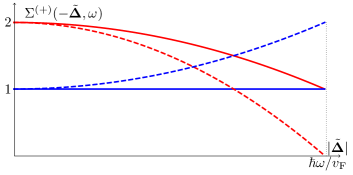
Figure 7: Cuts of the cross-section for a coupling $\mathbf{F}^{0}=\bm{0}$ and $\text{F}_{i\,j}={\delta}_{i\,j}$. The cross-section is plotted as a function of $\lvert{\tilde{\bm{\Delta}}}\rvert$ for scattering between nodes of chirality $\chi_{f}=-(+)\chi_{i}$ in blue (red) along $\theta_{{\tilde{\bm{\Delta}}}}=\pi/2$ ($\theta_{{\tilde{\bm{\Delta}}}}=0$) in full (dashed) lines.

The angular dependence of the cross-section of unpolarized neutrons results from a combination of two facts: first, the electron polarization is dependent on the transferred momentum, and second, the $\text{F}_{ij}^{\perp}$ is anisotropic so it is possible to see the variation of the electron-polarization even with unpolarized neutrons. If, hypothetically it had been the case that $\text{F}^{\perp}_{i\,j}={\delta}_{i\,j}$, then the cross-section would have no angular ${\tilde{\bm{\Delta}}}$ dependence, but would be spherical symmetric as a function of $|{\tilde{\bm{\Delta}}}|$ for a given $\omega$. However, $\text{F}_{\perp}$ can never be diagonal because in a coordinate system where $\widehat{\mathbf{k}}_{0}=\hat{\mathbf{z}}$, $\text{F}_{\perp}$ would have two columns orthogonal to $\widehat{\mathbf{k}}_{0}$ because $\mathbf{F}^{i}_{\perp}\cdot\widehat{\mathbf{k}}_{0}=0$ holds always. This generally implies angular dependence. However, although this condition rules out $\text{F}^{\perp}_{i\,j}={\delta}_{i\,j}$, there is a way that the spin-momentum locking could be hidden in the time-reversal symmetric case. The coupling

$$\text{F}_{\perp}=\begin{pmatrix}1&0&0\\ 0&1&0\\ i&0&0\end{pmatrix},$$ (30)

gives a cross-section $\pi\Sigma^{(+)}(\mathbf{q},\omega)=\sum_{j=1}^{3}\chi^{\prime\prime(+)}_{j\,j}(\mathbf{q},\omega)$, which has the same effect as if $\text{F}^{\perp}_{i\,j}={\delta}_{i\,j}$. Such a coupling is allowed, though probably not very likely to occur since it is very specific. Consequently, any angular dependence of the cross-section implies probing spin-momentum locking. The reverse statement is necessarily true for inversion-symmetric nodes, whereas it is not necessarily true for time-reversal symmetric nodes. The strong angular ${\tilde{\bm{\Delta}}}$ dependence of the cross-section reflects that the spherical harmonics Eq. (17) and (19) change rapidly as a function of ${\tilde{\bm{\Delta}}}$. When $\omega$ is small, the cross-section varies just as strongly with the angle on the surface of the sphere $|{\tilde{\bm{\Delta}}}|=\hbar\omega/v_{\rm F}$. This is a large variation for a small change in momentum. That is because the Weyl particle and hole have their momentum locked to spin, or equivalently, it reflects the singularity of the wavefunctions $|\tilde{\mathbf{p}};\eta\chi\rangle$ at $\tilde{\mathbf{p}}=0$. This differs from scattering between two pockets of a narrow gap semiconductor, where there would be no angular ${\tilde{\bm{\Delta}}}$ dependence because the wavefunctions are continuous.

Figure 8: Comparison of cross-sections for different couplings. The cross-section $\Sigma^{(+)}(-{\tilde{\bm{\Delta}}},\omega)$ for scattering between inversion symmetric nodes is plotted in isotropic coordinates ${\tilde{\bm{\Delta}}}$ for a given energy transfer $\hbar\omega$. Columns are cuts of $|{\tilde{\bm{\Delta}}}|$ with the left, middle, and right columns at $|{\tilde{\bm{\Delta}}}|v_{\rm F}/\hbar\omega=0.2,0.5$, and $0.95$, respectively. All rows are the same case of coupling eigendirections, Eq. (21a), $\widehat{\mathbf{a}}_{1}=\hat{\mathbf{x}}$ and $\widehat{\mathbf{a}}_{2}=\hat{\mathbf{y}}$ but different eigenvalues $\alpha_{1}$ and $\alpha_{2}$ and constant $\text{F}^{0}_{\perp}$. The upper row [8,8,8] is for $\text{F}^{0}_{\perp}=0$ and $\alpha_{1}=\alpha_{2}=1$, The middle row [8,8,8] is for $\text{F}^{0}_{\perp}=0$ and $\alpha_{1}=2\alpha_{2}=1$. The lower row [8,8,8] is for $\text{F}^{0}_{\perp}=1/2$ and $\alpha_{1}=2\alpha_{2}=1$. Intensity is given by the temperature scale in subfigure 8.

V.3 Universal features of the cross-section with an unpolarized detector

The form of the cross-section can change a great deal depending on the values of the coupling parameters, suggesting in particular that it might not be possible to observe the chiralities at the two Weyl nodes, or even whether they are the same or different. With an unpolarized detector one loses information about how the neutron’s spin is affected by coupling to the electron so the situation is worse.

To understand the situation better, both theoretically and experimentally, a result that is independent of sample-parameters is desirable (e.g., a sum-rule). However the usual sum-rules involve sums over all bands, obscuring the relevant low energy physics of a WSM. However, by taking the ratio of spherically averaged cross-sections we will get a prediction, which for time-reversal symmetric nodes (see Sec. V.3.1 and V.3.2) is a universal expression capturing only the relevant relativistic Weyl fermion physics measured in internode scattering. Hence this expresses exactly the information we seek from a sum-rule. For inversion symmetric nodes (see Sec. V.3.3), the averaging method does not lead to a completely universal expression, because of the coupling $\mathbf{F}^{0}$ may be present in this case. However, there is another universal property of the cross-section.

V.3.1 Time-reversal symmetric Weyl nodes: Unpolarized incident neutrons

Time-reversal symmetry has two consequences: the chiralities of the Weyl nodes is the same, and the couplings are restricted by Eq. (22). The inelastic cross-section Eq. (20) is determined by Eq. (17). In spite of the large number of coupling parameters, the averaging method mentioned above gives some universal predictions, and these reflect the two nodes’s handedness being identical. On the other hand, the chirality cannot be measured. The chirality appears only in the $\chi^{\prime\prime i\,0}_{(+)}$ ($i=1,2,3$) components of the susceptibility, but since $\mathbf{F}^{0}_{\perp}=\bm{0}$, such terms do not appear in the cross-section.

For unpolarized incident neutrons Eq. (20a) is

$$\Sigma^{(+)}(\mathbf{q},\omega)=\frac{a}{\pi}\mathbf{F}^{i,*}_{\perp}\cdot\mathbf{F}^{j}_{\perp}[\{\left(\hbar\omega/v_{\rm F}\right)^{2}-|{\tilde{\bm{\Delta}}}|^{2}\}{\delta}_{ij}+\tilde{\Delta}_{i}\tilde{\Delta}_{j}].$$ (31)

The tensor $\chi^{\prime\prime ij}_{(+)}$ has no antisymmetric part, so it consists only of terms that transform as a spherical tensor with angular momentum $l=0$ and $2$.

As previously stated, we can extract information by averaging the cross-section Eq. (31) over the solid angle One must do this average with respect to ${\tilde{\bm{\Delta}}}=T\bm{\Delta}$, in which the dispersion is isotropic. In terms of the original coordinates this is an average over an ellipsoid. Averaging gives $\left<\pi\Sigma^{(+)}(\mathbf{q},\omega)\right>=a[\left(\hbar\omega/v_{\rm F}\right)^{2}-\frac{2}{3}\lvert{\tilde{\bm{\Delta}}}\rvert^{2}]\left(\alpha_{1}+\alpha_{2}\right)$ where all the sample-specific information $\alpha_{1,2}$ factors out. Hence, we can divide by $\left<\Sigma^{(+)}(\mathbf{q}^{\prime},\omega^{\prime})\right>_{4\pi}$ for any arbitrary reference (within the low energy window) $\mathbf{q}^{\prime}=2\mathbf{k}_{0}-{\tilde{\bm{\Delta}}}^{\prime}$ and $\omega^{\prime}$ to get a result independent of $\alpha_{1,2}$, i.e.,

$$\frac{\left<\Sigma^{(+)}(\mathbf{q},\omega)\right>_{4\pi}}{\left<\Sigma^{(+)}(\mathbf{q}^{\prime},\omega^{\prime})\right>_{4\pi}}=\frac{\left(\hbar\omega/v_{\rm F}\right)^{2}-(2/3)\lvert{\tilde{\bm{\Delta}}}\rvert^{2}}{\left(\hbar\omega^{\prime}/v_{\rm F}\right)^{2}-(2/3)\lvert{\tilde{\bm{\Delta}}}^{\prime}\rvert^{2}},$$ (32)

which is a universal function of ${\tilde{\bm{\Delta}}},{\tilde{\bm{\Delta}}}^{\prime},\omega$ and $\omega^{\prime}$ that are all controlled in experiment. For example, choosing the reference cross-section to be of same energy but with $\tilde{\Delta}=0$, the ratio of averaged cross-sections in ${\tilde{\bm{\Delta}}}$-coordinates centered on $2\mathbf{k}_{0}$ is

$$\frac{\left<\Sigma^{(+)}(-{\tilde{\bm{\Delta}}},\omega)\right>_{4\pi}}{\left<\Sigma^{(+)}(\bm{0},\omega)\right>_{4\pi}}=1-\frac{2}{3}\left(\frac{\lvert{\tilde{\bm{\Delta}}}\rvert}{\hbar\omega/v_{\rm F}}\right)^{2},$$ (33)

which is a universal function of ${\tilde{\bm{\Delta}}}$ and $\omega$ plotted in Fig. 9. In particular, the averaged cross-section before the jump is $\frac{1}{3}$ the cross-section at ${\tilde{\bm{\Delta}}}=0$. This is a combined result of the density of states decreasing by a factor of $\frac{2}{3}$ with increasing ${\tilde{\bm{\Delta}}}$ and the interaction matrix elements decreasing when the spins go from being antiparallel to parallel. This has to do with the fact that the interaction is more likely to flip than not to flip the electron spin, as explained in Sec. V.2 for the case $\text{F}^{i}_{j}\propto\delta_{ij}$. Note that the result surprisingly applies to any F after averaging.

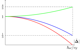
Figure 9: Universal predictions. The solid angle averaged cross-section ratio Eq. (33), (38), and (39) in blue, red, and green, respectively, as a functions of isotropic coordinate ${\tilde{\bm{\Delta}}}$.

V.3.2 Time-reversal symmetric Weyl nodes: Polarized incident neutrons

For polarized incident neutrons Eq. (20b) is

$$\pi\mathbf{P}\cdot\bm{\Sigma}^{\prime(+)}(\mathbf{q},\omega) = ia\,(\mathbf{P}\cdot\widehat{\mathbf{k}}_{0})\widehat{\mathbf{k}}_{0}\cdot(\mathbf{F}^{i,*}_{\perp}\times\mathbf{F}^{j}_{\perp})$$

$$\times [\{(\hbar\omega/v_{\rm F})^{2}-|{\tilde{\bm{\Delta}}}|^{2}\}{\delta}_{ij}+\tilde{\Delta}_{i}\tilde{\Delta}_{j}].$$

The cross-section for any material depends only on the component of $\mathbf{P}$ along $\mathbf{k}_{0}$; in fact, in any neutron scattering experiment the cross-section at low energies depends only on the component of $\mathbf{P}$ in the direction of the momentum transfer, because of the condition $\bm{\mathcal{J}}\cdot\bm{\Delta}\mathbf{k}=0$. We can take a ratio between any two solid angle averages of Eq. (V.3.2) to get a result independent of $\beta_{1,2}$, i.e.

$$\frac{\left<\mathbf{P}\cdot\bm{\Sigma}^{\prime(+)}(\mathbf{q},\omega)\right>_{4\pi}}{\left<\mathbf{P}^{\prime}\cdot\bm{\Sigma}^{\prime(+)}(\mathbf{q}^{\prime},\omega^{\prime})\right>_{4\pi}}=\frac{\mathbf{P}\cdot\widehat{\mathbf{k}}_{0}}{\mathbf{P}^{\prime}\cdot\widehat{\mathbf{k}}_{0}}\frac{\left<\Sigma^{(+)}(\mathbf{q},\omega)\right>_{4\pi}}{\left<\Sigma^{(+)}(\mathbf{q}^{\prime},\omega^{\prime})\right>_{4\pi}},$$ (35)

which is a universal function of $\mathbf{P},\mathbf{P}^{\prime},{\tilde{\bm{\Delta}}},{\tilde{\bm{\Delta}}}^{\prime},\omega$ and $\omega^{\prime}$ that are controlled in experiment. This function is that of Eq. (32) weighted by the ratio of polarization vectors’ projection onto the internode direction.

V.3.3 Inversion symmetric Weyl nodes: Unpolarized incident neutrons

For the inversion symmetric case, the inelastic cross-section Eq. (20) is determined by Eq. (19) and the coupling is restricted by Eq. (23). Two differences from the time-reversal symmetric case are that $\mathbf{F}^{0}$ can be nonzero which makes it more complicated to obtain a “universal prediction”. Furthermore, the chirality of the node where a hole is created can enter the cross-section through the antisymmetric part of the susceptibility $\chi^{\prime\prime i\,j}_{(+)}$ ($i,j=1,2,3$), which allows the chirality to be measured, although polarized neutrons and detectors are required for this. In this section, we will illustrate the use of the spectral decomposition of the effective coupling Eq. (21).

For unpolarized incident neutrons Eq. (20a) is

$$\pi \Sigma^{(+)} (\mathbf{q},\omega)=\alpha_{0}\frac{3a}{2}[\left(\hbar\omega/v_{\rm F}\right)^{2}-\lvert{\tilde{\bm{\Delta}}}\rvert^{2}]$$

$$+ \frac{a}{2}\sum_{m=1}^{2}\,\alpha_{m}\,[\left(\hbar\omega/v_{\rm F}\right)^{2}+\lvert{\tilde{\bm{\Delta}}}\rvert^{2}-2|{\tilde{\bm{\Delta}}}\cdot\hat{\mathbf{a}}_{m}|^{2}],$$

where $\hat{\mathbf{a}}_{1,2}$ are the two orthogonal, real unit vectors from the spectral decomposition of F, and $\alpha_{1,2}$ are the corresponding parameters as in Eq. (21a). In this expression appears a term $\alpha_{0}=\mathbf{F}^{0}_{\perp}\cdot\mathbf{F}^{0}_{\perp}$ which is generically nonzero. This term gives a $\chi^{\prime\prime 0\,0}_{(+)}$ contribution to the cross-section with no angular ${\tilde{\bm{\Delta}}}$ dependence. As $\chi^{\prime\prime i\,0}_{(+)}=0$ and $\mathbf{F}^{i}_{\perp}\cdot\mathbf{F}^{j}_{\perp}$ is symmetric in spin-indices, only the symmetric part of $\chi^{\prime\prime i\,j}_{(+)}$ contributes, which we have seen does not depend on $\chi$. It is therefore not possible to measure the chirality of the nodes with unpolarized neutrons.

The cross-section Eq. (V.3.3) is plotted in Fig. 8 as a function of ${\tilde{\bm{\Delta}}}$ for the case where coupling eigendirections of Eq. (21a) are $\widehat{\mathbf{a}}_{1}=\hat{\mathbf{x}}$ and $\widehat{\mathbf{a}}_{2}=\hat{\mathbf{y}}$ for various values of $\alpha_{0,1,2}$. Figure 10 plots cuts of the cross-section plotted in Fig. 8,8 and 8, from which one sees that the intensity variation is substantial. The $4$-band toy model (see Sec. III.2) corresponds to couplings with $\widehat{\mathbf{a}}_{1}=\hat{\mathbf{x}}$, $\widehat{\mathbf{a}}_{2}=\hat{\mathbf{y}}$, $\alpha_{1}=\alpha_{2}=\text{F}_{\perp,xx}^{2}$ and $\alpha_{0}=0$, the cross-section of which therefore has the same angular dependence as the top row of Fig. 8 but the intensity is a factor $2\text{F}_{\perp,xx}^{2}$ amplified by the value in Fig. 4.

The angular average of Eq. (V.3.3) is

$$\left<\pi\Sigma^{(+)}(\mathbf{q},\omega)\right>_{4\pi} = \alpha_{0}\frac{3a}{2}[\left(\hbar\omega/v_{\rm F}\right)^{2}-\lvert{\tilde{\bm{\Delta}}}\rvert^{2}]$$

$$+ \frac{a}{2}[\left(\hbar\omega/v_{\rm F}\right)^{2}+\lvert{\tilde{\bm{\Delta}}}\rvert^{2}/3]\left(\alpha_{1}+\alpha_{2}\right),$$

where the sample specific information $\alpha_{0,1,2}$ does not factor out. Hence we cannot divide by $\left<\Sigma^{(+)}(\mathbf{q}^{\prime},\omega^{\prime})\right>_{4\pi}$ for any arbitrary reference $\mathbf{q}^{\prime}$ and $\omega^{\prime}$ to get a universal result independent of $\alpha_{0,1,2}$. However, if the coupling $\mathbf{F}_{\perp}^{i}=\mathbf{0}$ vanish for all $i=1,2,3$ then $\alpha_{1,2}=0$ and we can get a result independent of $\alpha_{0}$. For example, choosing the reference cross-section to be of same energy but direct internode scattering, the ratio of averaged cross-sections in ${\tilde{\bm{\Delta}}}$-coordinates centered on $2\mathbf{k}_{0}$ is

$$\frac{\left<\Sigma^{(+)}(-{\tilde{\bm{\Delta}}},\omega)\right>_{4\pi}}{\left<\Sigma^{(+)}(\bm{0},\omega)\right>_{4\pi}}=1-\left(\frac{\lvert{\tilde{\bm{\Delta}}}\rvert}{\hbar\omega/v_{\rm F}}\right)^{2},$$ (38)

which is a monotonically attenuating function plotted in Fig. 9. If, on the other hand, the coupling $\mathbf{F}_{\perp}^{0}=\bm{0}$ vanishes then $\alpha_{0}=0$ and we can get a result independent of $\alpha_{1,2}$. For example, choosing the reference dataset to be the same as above, the ratio of averaged cross-sections in ${\tilde{\bm{\Delta}}}$-coordinates centered on $2\mathbf{k}_{0}$ is

$$\frac{\left<\Sigma^{(+)}(-{\tilde{\bm{\Delta}}},\omega)\right>_{4\pi}}{\left<\Sigma^{(+)}(\bm{0},\omega)\right>_{4\pi}}=1+\frac{1}{3}\left(\frac{\lvert{\tilde{\bm{\Delta}}}\rvert}{\hbar\omega/v_{\rm F}}\right)^{2},$$ (39)

which is a monotonically increasing function plotted in Fig. 9. Hence the ratio with $\alpha_{1,2}=0$ can be distinguished from the ratio with $\alpha_{0}=0$. In the general case with $\alpha_{0,1,2}\neq 0$ one does not obtain a universal ratio of solid angle averaged cross-sections. Although Eq. (V.3.3) is non-universal, the functional dependence, $c_{1}(\hbar\omega/v_{\rm F})^{2}+c_{2}|{\tilde{\bm{\Delta}}}|^{2}$ with constants $c_{1,2}$ is very specific.

In fact, there is a more quantitative universal prediction as well. Eq. (V.3.3) can be written as

$$\pi\Sigma^{(+)}(\mathbf{q},\omega)=\frac{\bar{\alpha}a}{2}\left[(\hbar\omega/v_{F})^{2}+\sum_{m=1}^{3}c_{m}({\tilde{\bm{\Delta}}}\cdot\hat{\mathbf{a}}_{m})^{2}\right],$$ (40)

where $\bar{\alpha}$ and $c_{i}$’s are certain parameters and $\hat{\bm{a}}_{3}$ is a unit vector completing a basis with $\hat{\mathbf{a}}_{1}$ and $\hat{\mathbf{a}}_{2}$; i.e., it is the direction in pseudospin space that is not coupled to the neutron spin. That such a direction exists follows from the fact that there is a direction in neutron spin space that is not coupled to the pseudospin, as seen more formally in the derivation of the spectral decomposition, see Sec. IV. Eq. (40) follows from $|{\tilde{\bm{\Delta}}}|^{2}=\sum_{m=1}^{3}({\tilde{\bm{\Delta}}}\cdot\hat{\mathbf{a}}_{m})^{2}$. The ${\tilde{\bm{\Delta}}}$-dependence of this expression is a quadratic function of ${\tilde{\bm{\Delta}}}$; although with respect to the $\hat{\mathbf{a}}$ basis it is diagonal, in the coordinate system of the experiment, it could be an arbitary quadratic function of ${\tilde{\bm{\Delta}}}$. Consider the cross-section at the maximum possible transfer momentum, $|{\tilde{\bm{\Delta}}}|=\hbar\omega/v_{\rm F}$. A quadratic form on the surface of a sphere has two maxima, two minima and two saddle-points (at diametrically opposite pairs of points). The prediction is that, the cross-section always has the property that the value at the maximum is the sum of the value at the saddle point and the minimum. In fact, the extrema always correspond to the eigendirections of the quadratic form, namely $\hat{\mathbf{a}}_{1},\hat{\mathbf{a}}_{2}$ and $\hat{\mathbf{a}}_{3}$. The values of the cross-sections at these points are $2\alpha_{2}(\hbar\omega/v_{\rm F})^{2}$, $2\alpha_{1}(\hbar\omega/v_{\rm F})^{2}$, and $2(\alpha_{1}+\alpha_{2})(\hbar\omega/v_{\rm F})^{2}$ respectively. The last is the largest since $\alpha_{1},\alpha_{2}\geq 0$. This prediction can be understood qualitatively by noting that the initial and final spins of the electron are antiparallel to one another. Hence there is no contribution to the cross-section at maximal $|{\tilde{\bm{\Delta}}}|$ due to the $\mathbf{F}^{0}$ coupling, which does not cause spin flips, while the cross-section due to the other interactions is greatest when the momentum is along $\mathbf{\hat{a}}_{3}$ because the neutron couples to both components of the spin perpendicular to this, namely $\hat{\mathbf{a}}_{1}$ and $\hat{\mathbf{a}}_{2}$ and so each term in the interaction induces the spin and also the momentum to flip.

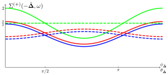
Figure 10: Angular variation of cross-section for different couplings. The cross-section for scattering between inversion symmetric nodes at a given energy transfer $\hbar\omega$ is plotted as a function angles $\phi_{{\tilde{\bm{\Delta}}}}$ and $\theta_{{\tilde{\bm{\Delta}}}}$ on a sphere with radius $|{\tilde{\bm{\Delta}}}|=0.95\hbar\omega/v_{\rm F}$. The green, blue, and red curves corresponds to that of Fig. 8, 8,8, respectively, as a function of $\theta_{{\tilde{\bm{\Delta}}}}$ at $\phi_{{\tilde{\bm{\Delta}}}}=\pi/4$, whereas the dashed curves are functions of $\phi_{{\tilde{\bm{\Delta}}}}$ at $\theta_{{\tilde{\bm{\Delta}}}}=\pi/4$.

V.3.4 Inversion symmetric Weyl points: Polarized incident neutrons

For polarized incident neutrons Eq. (20b) is

$$\pi \mathbf{P} \cdot\bm{\Sigma}^{\prime(+)}(\mathbf{q},\omega)$$ (41)

$$= -\chi a\left(\hbar\omega/v_{\rm F}\right)\mathbf{P}\cdot(\mathbf{F}^{i}_{\perp}\times\mathbf{F}^{j}_{\perp})\epsilon_{ijk}\tilde{\Delta}_{k}.$$

Despite the possibility that $\mathbf{F}_{\perp}^{0}\neq\bm{0}$ there is no $\chi^{\prime\prime 0\,0}_{(+)}$ contribution because $\widehat{\mathbf{k}}_{0}\cdot\mathbf{F}^{0}_{\perp}\times\mathbf{F}^{0}_{\perp}=0$. As $\chi^{\prime\prime i\,0}_{(+)}=0$ and $\mathbf{F}^{i}_{\perp}\times\mathbf{F}^{j}_{\perp}$ is antisymmetric in spin-indices, only the antisymmetric part of $\chi^{\prime\prime i\,j}_{(+)}$ contributes, which is a term that transforms as a spherical tensor with angular momentum $l=1$. From the antisymmetric part of $\chi^{\prime\prime i\,j}_{(+)}$ one sees that this measures “chiral” fluctuations $\langle{\bm{\sigma}}(\mathbf{q},\omega)\times{\bm{\sigma}}(-\mathbf{q},-\omega)\rangle\cdot{\tilde{\bm{\Delta}}}$ originating in the axial-vector of the interaction.

Now $\mathbf{F}^{i}_{\perp}\times\mathbf{F}^{j}_{\perp}$ is always parallel to $\mathbf{k}_{0}$. This implies $(\mathbf{F}^{i}_{\perp}\times\mathbf{F}^{j}_{\perp})\cdot\mathbf{P}$ depends only on the component of $\mathbf{P}$ in the internode direction $\mathbf{k}_{0}$; further it is antisymmetric between $i$ and $j$, hence it can be written $\epsilon_{ijk}\gamma_{k}(\mathbf{P}\cdot\hat{\mathbf{k}}_{0})$, for some numbers $\gamma_{k}$. (Explicitly, $\gamma_{3}=\hat{\mathbf{k}}_{0}\cdot(\mathbf{F}_{1}\times\mathbf{F}_{2}$, etc.) Hence

$$\pi\mathbf{P}\cdot\bm{\Sigma}^{\prime(+)}(\mathbf{q},\omega) = -\chi a\left(\hbar\omega/v_{\rm F}\right)(\bm{\gamma}\cdot{\tilde{\bm{\Delta}}})(\mathbf{P}\cdot\hat{\mathbf{k}}_{0}).$$ (42)

This part is linear in ${\tilde{\bm{\Delta}}}$, so the angular average is

$$\left<\mathbf{P}\cdot\bm{\Sigma}^{\prime(+)}(\mathbf{q},\omega)\right>_{4\pi}=0.$$ (43)

Now although this result depends on the chirality, the coefficients $\gamma_{i}$ are not known because they depend on F, so it is not possible to measure the chirality even with polarized neutrons when the detector is unpolarized. The next section explains that the polarization-independent and dependent cross-sections $\Sigma^{(+)},\bm{\Sigma}^{\prime(+)}$ are not enough to determine $\chi$; there is always at least one choice of F that matches the data for each of $\chi=\pm 1$.

V.4 Polarized measurement

We will now consider polarized neutrons and detector; the main result is that it is possible to measure the chirality for inversion-symmetric WSMs.

V.4.1 Pure States of Scattered Neutrons

Consider directing an incident fully polarized beam of neutrons with polarization vector $\mathbf{P}^{i}$ on a WSM and measuring the polarization vector $\mathbf{P}^{f}$ of the scattered beam. The Blume-Maleyev polarization matrix describes the relationship between them. Instead of calculating this, we simplify the discussion and consider, for the moment, a single incident neutron in spin state $\lvert\tau_{i}\rangle$ and measuring whether the scattered neutron is in the state $\lvert\tau_{f}\rangle$ or in the orthogonal one.

The Weyl states are not eigenvectors of $\sigma_{z}$, but are dependent on the direction and magnitude of ${\tilde{\bm{\Delta}}}$. For a given scattering process, i.e. a fixed initial and final neutron state, the cross-section Eq. (13) sums up all internal particle-hole pair Weyl states which fulfill the energy and momentum constraints of the system (see Fig. 5). Intuitively one expects that each of these pairs affects the scattered neutron in a different way.

For small amounts of transferred momentum it is correct (as this reasoning suggests) that the scattered neutron will be in a mixed state. However, consider the case where the momentum transfer is the maximum that is possible for the given energy transfer, $|{\tilde{\bm{\Delta}}}|=\hbar\omega/v_{\rm F}$. For a given pure initial spin state of the neutron and a fixed momentum transfer, the cross-section can be shown (see below) to take the form $\frac{\text{d}^{2}\sigma(\mathbf{q},\omega)}{\text{d}\Omega\text{d}E_{f}}\big{|}_{\tau_{i}}^{\tau_{f}}\propto\left|\langle\tau_{f}|\phi\rangle\right|^{2}$ where the auxiliary state $|\phi\rangle$ depends on the initial neutron state $\lvert\tau_{i}\rangle$ and direction ${\tilde{\bm{\Delta}}}$. In other words, the scattered neutron is in a pure state $|\phi\rangle$. This can be demonstrated experimentally by measuring that there is a certain final state for which the scattering rate into that state is zero. This final neutron state is the time-reversed ket of $\rvert\phi\rangle$, i.e. $\lvert\tau_{f}^{\rm TR}\rangle=T\lvert\phi\rangle$, since $\langle\tau_{f}^{\rm TR}|\phi\rangle=0$.

The fact that there is only one transition available for a given momentum transfer is direct evidence of spin-momentum locking. The reason for the perfect polarization, in more detail, is that in the extreme limit $|\tilde{\bm{\Delta}}|\approx\hbar\omega/v_{\rm F}$, the set of possible internal momenta degenerates from an ellipsoid to a line. All the possible values are parallel and thus the electron and hole spin states are the same throughout the particle-hole continuum. The current matrix element is the same for all pairs, so the integral over the state of the electrons and holes just gives a multiplicative factor and the cross section is proportional to

$$\frac{d\sigma}{d\Omega}\propto|\langle\tau_{f};\chi_{f};-\widehat{{\tilde{\bm{\Delta}}}}|\bm{\tau}\cdot\bm{\mathcal{M}}|\widehat{{\tilde{\bm{\Delta}}}};-\chi_{i};\tau_{i}\rangle|^{2}$$ (44)

where the magnetization $\bm{\mathcal{M}}$ is given by Eq. (10) and $\bm{\tau}$ is, as above, the neutron spin operator. The dynamics of the neutron spin may be understood as a precession of the neutron in a magnetic field that depends on how the electron transitions. To see this, we factor this expression as $|\langle\tau_{f}|\bm{\tau}|\tau_{i}\rangle\cdot\langle\chi_{f};-\widehat{{\tilde{\bm{\Delta}}}}|\bm{\mathcal{M}}|\widehat{{\tilde{\bm{\Delta}}}};-\chi_{i}\rangle|^{2}$, then define the c-number $\bm{\mathcal{M}}_{fi}=\langle\chi_{f};-\widehat{{\tilde{\bm{\Delta}}}}|\bm{\mathcal{M}}|\widehat{{\tilde{\bm{\Delta}}}};-\chi_{i}\rangle$. The transition probability can now be written as $\frac{d\sigma}{d\Omega}\propto|\langle\tau_{f}|\bm{\tau}\cdot\bm{\mathcal{M}}_{fi}|\tau_{i}\rangle|^{2}$ Thus, we may define $|\phi\rangle=\bm{\mathcal{M}}_{fi}\cdot\bm{\tau}|\tau_{i}\rangle$, and the cross-section is given by $|\langle\tau_{f}|\phi\rangle|^{2}$ as claimed above. Intuitively, when the electron’s spin flips in a particular way, the scattered beam ends up in a fully polarized state if the beam was initially fully polarized; the final state is obtained by applying the operator $\bm{\mathcal{M}}_{fi}\cdot\bm{\tau}$ to the initial state. This mechanism is due to the constant energy contour degenerating into a line and to perfect spin-momentum locking; if there were curvature, the electron spinors would not be all aligned and the final neutron beam would not be fully polarized.

In a neutron experiment, in which a beam of $N\gg 1$ neutrons having a polarization $\mathbf{P}^{i}$ is incident to the target, all neutrons scattered to a certain momentum have the same available scattering channel $\lvert\phi\rangle=\bm{\mathcal{M}}_{fi}\cdot\bm{\tau}|\tau_{i}\rangle$ if the initial neutron beam is fully polarized. This state has an expansion

$$c_{1}=\langle\uparrow\rvert\phi\rangle/\lvert\phi\rvert\quad,\quad c_{2}=\langle\downarrow\rvert\phi\rangle/\lvert\phi\rvert.$$ (45)

The emitted neutrons in this direction are fully polarized and specified by $\mathbf{P}^{f}\cdot\bm{\tau}\lvert\tau_{f}\rangle=\lvert\tau_{f}\rangle$ where the polarization vector has the components

$${\text{P}}^{f}_{x}=2\Re\left[c_{1}^{*}c_{2}\right]\>,\>{\text{P}}^{f}_{y}=2\Im\left[c_{1}^{*}c_{2}\right]\>,\>{\text{P}}^{f}_{z}=|c_{1}|^{2}-|c_{2}|^{2}.$$ (46)

The polarization vector Eq. (46) is to be understood as a field $\mathbf{P}^{f}({\tilde{\bm{\Delta}}}/|{\tilde{\bm{\Delta}}}|)$ on the surface of the sphere of transferred maximum momentum. The matrix element of the magnetization can be evaluated explicitly for time-reversal and inversion symmetric nodes, $\bm{\mathcal{M}}_{fi}=\widehat{\tilde{\Delta}}_{i}\mathbf{F}^{i}_{\perp}$ and $\bm{\mathcal{M}}_{fi}=(\hat{u}_{j}+i\chi\hat{v}_{j})\mathbf{F}_{\perp}^{j}$, respectively. Here $\hat{\mathbf{u}},\hat{\mathbf{v}}$ are some pair of vectors making a right-handed coordinate system together with ${\tilde{\bm{\Delta}}}$. The total cross-section is proportional to $|\phi|^{2}$, which gives

$$|\phi|^{2} = \widehat{\tilde{\Delta}}_{i}\widehat{\tilde{\Delta}}_{j}(\mathbf{F}^{i,*}_{\perp}\cdot\mathbf{F}^{j}_{\perp}+\mathbf{P}^{i}\cdot\widehat{\mathbf{k}}_{0}i\widehat{\mathbf{k}}_{0}\cdot\mathbf{F}^{i,*}_{\perp}\times\mathbf{F}^{j}_{\perp}),\hskip 12.80365pt$$ (47a)

$$|\phi|^{2} = ({\delta}_{ij}-\widehat{\tilde{\Delta}}_{i}\widehat{\tilde{\Delta}}_{j})\mathbf{F}_{\perp}^{i}\cdot\mathbf{F}_{\perp}^{j}$$ (47b)

$$\hskip 1.42271pt-\chi\mathbf{P}^{i}\cdot\widehat{\mathbf{k}}_{0}\widehat{\tilde{\Delta}}_{k}\epsilon_{k\,i\,j}\widehat{\mathbf{k}}_{0}\cdot\mathbf{F}_{\perp}^{i}\times\mathbf{F}_{\perp}^{j},$$

for time-reversal and inversion symmetric nodes, respectively, in agreement with our general expressions [see Eqs. (31), (V.3.2), (V.3.3),(41)] for the cross-section in the case where $|{\tilde{\bm{\Delta}}}|=\hbar\omega$. Notice that $|\phi\rangle$ is not of unit norm.

Notice that in this result, the chirality $\chi$ appears only for inversion-symmetric nodes, suggesting that it is possible to measure the chirality for inversion-symmetric but not time-reversal symmetric materials. This is true as shown in the next section, but it is not possible to determine the chirality from a measurement of the total cross-section, although this formula seems to suggest it. The problem is that the $\mathbf{F}$ parameters are unknown. It is possible to compensate for a change in sign of $\chi$ by changing the $\mathbf{F}$’s. If two materials have scattering cross-sections as a function of $\tilde{\mathbf{\Delta}}$ that look the same except that the cross-section pattern is reflected through the $z$-axis (whenever neutrons polarized in the same way are passed through the material), then it looks as if the materials have the opposite sign of $\chi$. However, there is an alternative explanation: suppose $\mathbf{k}_{0}$ is parallel to the $z$-axis, $\hat{\mathbf{z}}\cdot\mathbf{F}^{i}=0$. If one material has $\mathbf{F}^{i}=\text{F}^{i}_{x}\hat{\mathbf{x}}+\text{F}^{i}_{y}\hat{\mathbf{y}}$ while the other has $\mathbf{F}^{i}=\text{F}^{i}_{x}\hat{\mathbf{x}}-\text{F}^{i}_{y}\hat{\mathbf{y}}$ for each $i$, this would also explain the reflection of the cross-section in the $xy$-plane.

To summarize, the scattering Eq. (47) is dependent on the initial neutron beam polarization vector, the scattering direction, and the a priori unknown coupling constants. Measuring the polarization vector of the final neutron beam at $|{\tilde{\bm{\Delta}}}|=\hbar\omega/v_{\rm F}$, one finds that $|\mathbf{P}^{f}|=1$ for all scattering directions and any incident fully polarized neutron beam. This is quite remarkable and counter-intuitive as one is probing particle-hole Weyl pairs and not conventional magnetic excitations.

V.4.2 Measuring Chiralities

It is possible to measure the chirality of the nodes in an inversion symmetric WSM, although it is not straightforward because of the unknown $\mathbf{F}$ parameters.

First, it is clear that it is not possible to measure the chirality for scattering between two nodes related by time-reversal symmetry, since the chirality does not appear in the cross-section, Eqs. (17) and (47a). This seems at first surprising since the two Weyl points are either both left-handed or right-handed, which should be distinguishable. One can understand why, nevertheless, it is impossible to distinguish them with neutron scattering from the following point of view: The scattering produces a particle-hole pair. The hole and particle at a Weyl point have the opposite handedness. So the two cases are essentially the same, with one excitation of each handedness in both cases. The only difference is how the charges of the excitations is correlated to their handedness. This does not affect the cross-section since the sign of the charge does not appear in the cross-section, which depends on the square of the matrix elements. On the other hand, in the inversion symmetric case, either two left-handed excitations are produced (if the Weyl point at $-\mathbf{k}_{0}$ is right-handed and the excitation at $+\mathbf{k}_{0}$ is left-handed) or two right-handed excitations are produced, explaining why $\chi$ enters into the cross-section. We will now explain how to measure the chirality in this case.

We will focus on the case discussed in the last section, where $|{\tilde{\bm{\Delta}}}|=\hbar\omega$. Because the spin and momentum of the electron are locked, we may ignore the momentum of the electron. We can simply consider the electron as fixed in space with a neutron scattering off of it. The expression for the cross-section, Eq. (44), is then interpreted as the cross-section for scattering in which the electron’s spin changes from $-\chi_{i}{\tilde{\bm{\Delta}}}$ to $-\chi_{f}{\tilde{\bm{\Delta}}}$, which is always a spin-flip scattering since $\chi_{i}=-\chi_{f}$. The interaction operator can be written $\bm{\tau}\cdot\bm{\mathcal{M}}=\tau_{x}(\mathbf{a}\cdot\bm{\sigma})+\tau_{y}(\mathbf{b}\cdot\bm{\sigma})$ where $a_{i}=\hat{\mathbf{x}}\cdot\mathbf{F}_{i},b_{i}=\hat{\mathbf{y}}\cdot\mathbf{F}_{i}$. No $z$-component appears because $\mathbf{k}_{0}\cdot\mathbf{F}_{i}=0$. The $\mathbf{F}_{0}$ term of $\mathcal{M}$ is omitted because it does not contribute to the matrix element for an event in which the electron’s spin flips.

One can do an experiment where one focuses on events where the neutron’s spin changes from a given $\lvert\tau_{i}\rangle$ to another $\lvert\tau_{f}\rangle$. If one could measure how the spin of the electron changes, one would expect (because of the form of the interaction above) a certain correlation of this measurement to the way the spin of the neutron has changed. Now an experiment actually measures how the momentum of the electron changes (by measuring momentum transfer), which is locked to the spin of the electron up to the sign that we wish to find. If the way the electron’s momentum changes is reversed from the behavior one expects from the spin, it must be because $\chi_{f}=-\chi_{i}=-1$ so that the spin is antiparallel to the momentum. If the interaction were $\sigma_{x}\tau_{x}+\sigma_{y}\tau_{y}$, this is clear; it is easy to work out how the electron’s spin is affected by scattering. With the arbitrary $\mathbf{a}$ and $\mathbf{b}$ the expectation of how the electron spin should flip would be distorted and it is not clear that it is possible to determine the sign of $\chi_{f},\chi_{i}$ if they are unknown.

In principle, we could prepare the neutron in any initial state and measure its final state along any axis. However, to trim the problem down, we will focus on just the rate of spin-flip scattering of the neutron. So consider an experiment where the neutron is prepared with a certain polarization direction $\hat{\mathbf{N}}$ and one measures the cross-section $f_{\hat{\mathbf{N}}}(\widehat{{\tilde{\bm{\Delta}}}})$ that it flips to $-\hat{\mathbf{N}}$ as a function of the direction of ${\tilde{\bm{\Delta}}}$. First consider the case where $|\mathbf{a}|=|\mathbf{b}|$ and they are orthogonal to one another for simplicity. We will calculate the probability as a function of the direction of the initial spins of the neutron and electron, $\hat{\mathbf{N}}$ and $\hat{\mathbf{E}}$ respectively (rather than momentum); the relation is $\hat{\mathbf{E}}=-\chi_{i}\widehat{{\tilde{\bm{\Delta}}}}$. One can evaluate $|\langle-\hat{\mathbf{N}},-\hat{\mathbf{E}}|\mathbf{a}\cdot\bm{\sigma}\tau_{x}+\mathbf{b}\cdot\bm{\sigma}\tau_{y}|\hat{\mathbf{E}},\hat{\mathbf{N}}\rangle|^{2}$ by means of the formula given in the previous section, $\langle-\hat{\mathbf{n}}|\bm{\sigma}|\hat{\mathbf{n}}\rangle=\mathbf{u}+i\mathbf{v}$ where $|\hat{\mathbf{n}}\rangle$ is a spinor oriented along the $\hat{\mathbf{n}}$ direction of the Bloch sphere, and $\hat{\mathbf{u}}$ and $\hat{\mathbf{v}}$ are any unit vectors that make a right-handed coordinate system together with $\hat{\mathbf{n}}$. We apply this formula to both the electron and neutron by introducing vectors $\hat{\mathbf{u}}_{e},\hat{\mathbf{v}}_{e},\hat{\mathbf{u}}_{n},\hat{\mathbf{v}}_{n}$. The probability of the electron flipping from $\hat{\mathbf{E}}$ to $-\hat{\mathbf{E}}$ and the neutron flipping from $\hat{\mathbf{N}}$ to $-\hat{\mathbf{N}}$ comes out to be

$$f_{\hat{\mathbf{N}}}(\widehat{{\tilde{\bm{\Delta}}}})\propto({\rm N}_{x}{\rm E}_{a}+{\rm N}_{y}{\rm E}_{b})^{2}+({\rm N}_{z}-{\rm E}_{c})^{2}$$ (48)

where ${\rm E}_{a},{\rm E}_{b},{\rm E}_{c}$ are the components of $\hat{\mathbf{E}}$ along the directions of $\mathbf{a},\mathbf{b}$ and a third direction making a coordinate system with them, $\hat{\mathbf{c}}=\hat{\mathbf{a}}\times\hat{\mathbf{b}}$.

A striking effect is that for any direction of the initial neutron spin, there are two initial spin directions of the electron for which spin-flips of the neutrons have zero probability. Thus in an experiment, one can map out the cross-section for a neutron spin-flip with a fixed $\hat{\mathbf{N}}$ as a function of momentum transfer and then search for these nodes. If the initial spin of the neutron is in the $xy$-plane, the two nodes of $f_{\widehat{\hat{\mathbf{N}}}}$ are in the $ab$ plane at opposite points of the equatorial circle. As the neutron spin rotates in the $xy$-plane the nodes of the electron spin rotate in the $ab$ plane. The corresponding nodes of the electron spin are related to $\hat{\mathbf{N}}$ as follows. Rotate the $xy$-plane onto the $ab$-plane so that $\hat{\mathbf{x}}$ maps to $\hat{\mathbf{a}}$ and $\hat{\mathbf{y}}$ maps to $\hat{\mathbf{b}}$. The initial neutron spin maps to a certain point on the great circle in the $ab$-plane and the two points $90^{\circ}$ away from this point on the great circle are the nodes. This follows from Eq. (48) by noting that $f$ is zero if ${\rm E}_{a}=\pm{\rm N}_{y}$; ${\rm E}_{b}=\mp{\rm N}_{x}$, ${\rm E}_{c}=0$. Comparing this prediction to experimental data would allow one to determine the directions of the $\hat{\mathbf{a}}$ and $\hat{\mathbf{b}}$ vectors up to a common sign.

Now if the neutron spin is moved out of the $xy$-plane, the nodes for the electron move out of the $ab$-plane, as $f=0$ when ${\rm E}_{c}={\rm N}_{z}$ and ${\rm E}_{a}/{\rm E}_{b}=-{\rm N}_{y}/{\rm N}_{x}$. Note that these nodes are not antipodal to one another: they both move into the same hemisphere, toward the $\hat{\mathbf{c}}$-axis.

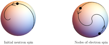
Figure 11: How to measure chirality. Consider scattering with a maximal $|{\tilde{\bm{\Delta}}}|$. For each initial spin of the neutron find the momentum transfer direction where spin-flip scattering has zero cross-section. There are always two such nodes. At the left is a sphere representing the possible initial spin directions of the neutron; as the spin moves along a spiral from the equator perpendicular to $\mathbf{k}_{0}$ up to one of the axes parallel to $\mathbf{k}_{0}$, the corresponding nodes (shown on the right) also spiral in some direction, with an arbitrary rotation and possibly a distortion due to the interaction parameters. However, no matter what the parameters are, if the nodes form a double-spiral with the same handedness as the neutron-spin’s spiral, then the scattering is from a right-handed to a left-handed Weyl point, and if with the opposite handedness, then the scattering is from a left-handed to a right-handed Weyl point.

To describe this in a geometrical way that is independent of knowing $\hat{\mathbf{a}},\hat{\mathbf{b}},\hat{\mathbf{c}}$ and their signs correctly, return to the first case where the neutron spin is rotating around the $xy$-plane and the electron nodes are rotating around the $ab$-plane. Find from which hemisphere of the electron’s Bloch sphere the nodes can be seen rotating with the same handedness as the neutron’s initial spin rotates when seen from the positive $z$-axis. That is the hemisphere the nodes will move into. Figure 11 illustrates this: if the neutron’s initial spin follows a helix starting on the great circle in the $xy$-plane and spirals in toward the $z$-axis, the two nodes for the electron’s initial spin both form a helix of the same handedness contracting towards one of the poles of the Bloch sphere.

Now in the neutron scattering experiment one measures $\widehat{{\tilde{\bm{\Delta}}}}$ rather than $\bm{\sigma}$. $\widehat{{\tilde{\bm{\Delta}}}}$ is parallel to the initial spin if $\chi_{f}=1$ and to the final spin if $\chi_{f}=-1$. Hence if $\chi_{f}=1$, the helix formed by the nodes has the same handedness as the helix which the neutron’s spin is made to rotate along, and it has the opposite handedness if $\chi_{f}=-1$.

The fact that the nodes move into the same hemisphere when the neutron’s spin moves out of the $xy$-plane can be understood by noting that $\tau_{x}\sigma_{a}+\tau_{y}\sigma_{b}$ is an ordinary “easy-axis” coupling of two spins, except that each is measured relative to its own coordinate system. So the sum of the component of each spin along the axis perpendicular to the plane where the coupling is, $\sigma_{c}+\tau_{z}$, should be conserved; if the neutron flips from up to down it is not possible for the electron spin to also flip from up to down, since then the net spin would change by $2\hbar$. It is surprising that there is a correlation between flips of the neutron’s spin along the $z$-axis and flips of the electron’s spin along the $c$-axis, since these components of spin do not appear in the interaction Hamiltonian. The direction of the $c$-axis is determined however by the relation $\sigma_{c}=i\sigma_{a}\sigma_{b}$.

As a brief remark on how to carry out such an experiment, it might seem as if measuring the nodes in the cross-section as a function of momentum-transfer for three polarizations of the neutrons, along the $x$, $y$, and $z$ axis, should be sufficient. This seemingly allows one to determine the momentum directions that are locked to the $a$,$b$ and $c$ axes of spin and whether they are right- or left-handed. However, the nodes for initial neutron spin $\hat{\mathbf{x}},\hat{\mathbf{y}}$ are at $\pm\hat{\mathbf{b}}$ and $\pm\hat{\mathbf{a}}$, so it is not possible to determine the signs of these axes, leaving the handedness indeterminate. This is solved by identifying the nodes for a few additional spin directions intermediate between $\hat{\mathbf{x}}$ and $\hat{\mathbf{y}}$.

If $\mathbf{a}$ and $\mathbf{b}$ are more general (not orthogonal and with different magnitudes), the same routine would allow one to measure the chirality; the only difference is that the nodes of the electron’s spin do not slide all the way to the $c$-axis when the spin of the neutron moves to the $z$-axis–they still spiral with the same handedness though.

VI Conclusion

In this paper, we have shown that INS can probe bulk excitations of type-$1$ Weyl nodes. These where assumed to be aligned at (or near) the chemical potentialRuan et al. (2016); Buchhold et al. (2018); Nandkishore et al. (2014); Huang et al. (2013); Skinner (2014); Syzranov et al. (2015) with realistic anisotropy, but a negligible scalar term $\alpha$. Footnote [$40$] outlines how any $|\alpha|<1$ is analytically tractable.

The analysis separated the cross-section into a Lorentz invariant susceptibility and a symmetry breaking coupling of neutrons to Weyl fermions determined by material specific $g$-factors. This had advantages: first, Lorentz invariant properties of the susceptibility, describing the excitations’ dynamics, are reflected in the cross-section. This leads to several universal quantitative predictions, and furthermore, the possibility of measuring chirality for inversion symmetric nodes despite arbitrary material parameters. Noticeably, the chirality of a Weyl point can be seen through the distortions produced by the unknown form of the neutron-electron interaction, which reflects its topological character. Secondly, anisotropy of these $g$-factors is actually helpful, as they render spin-momentum locking observable even in a fully unpolarized experiment. Furthermore, the $g$-factors can enhance the cross-section intensity as they, in principle, can take any value from zero to diverging, which differs from the bare coupling value $g/2=1$. As a proof of concept, we estimated the intensity under optimistic conditions $\text{q}_{i}/\text{q}_{f}\times\text{d}^{2}\sigma^{(+)}(\mathbf{q},\omega)/\text{d}\Omega\text{d}E_{f}\lesssim 2\times 10^{-2}\;{\rm mb}/{\rm meV\,f.u.\,sr}$ for a toy model. This is low but remarkably only of order $10^{-2}-1$ smaller than what has been observed in scattering off spin-$\frac{1}{2}$ particle-hole pairsGoremychkin et al. (2018); Vignolle et al. (2007); Walters et al. (2009); Fujita et al. (2012); Janoschek et al. (2015).

INS can thus provide a platform to understand the intrinsic behavior of WSMs, for example, the spin and orbital effects discussed here. It can test the form of the Weyl equation in materials, including monitoring changes in it such as relocation in energy and momentum space, distortion of dispersion, redistribution of occupation numbers, due to applied fields, currents or elastic and magnetic deformations as predicted Ref. Chan et al., 2016; Ghorashi et al., 2018; Cortijo et al., 2015; Ghimire et al., 2019; Araki, ; Sekine et al., 2017.

Some of the details that have appeared in this study could give new information about Weyl materials. For example, the many $g$-factors describing the emergent magnetic moment of the Weyl fermions induced by an external magnetic field (which does not have to be from a neutron). In particular, it would be interesting to know how these parameters evolve as a magnetic Weyl semimetal approaches the transition pointCrippa et al. (2020); Chang and Coleman (2018); Wan et al. (2011); Ivanov et al. (2019). The $4$-band model above shows that they depend on the strength of the spontaneous magnetic ordering and hybridization between bands. Such an endeavor can be done theoretically by use of numerically realistic band structure calculations and experimentally be measured by neutron scattering.

Besides the specific problem of neutron scattering, particle-hole correlators (as calculated here) are relevant to WSMs’ intrinsic properties. For example, particle-hole bound states (like plasma waves) might form, and their self-energy is closely related to the spin-susceptibility. If a particle-hole bound state from excitations at distinct Weyl points can form, we would expect angle-dependent properties, for example, it should have an effective mass that is proportional to the matrix elements between the two Weyl points and hence would be strongly momentum dependent. Also, just as there is an emergent magnetic moment of Weyl excitations, there could be an emergent electric dipole moment, which is not ruled out by symmetry unlike the case of an electron in free spaceI.B. Khriplovich (1997). This could influence the bound state through pseudospin dipole-dipole interactions. It is necessary to understand carefully what properties of Weyl fermions are universal for such analyses, and the relativistic method developed here should be useful.

Furthermore, it would be interesting to extend our method to derive the cross-section for scattering between emergent BdG Weyl nodes induced in a monopole superconducting WSMSun et al. (2019).

Appendix A Principal axis transformation

When the three parameters $\mathbf{v}_{0}^{(i)}$ of Eq. (2) are negligible, the total Hamiltonian is

$$H_{0} = \sum_{i=1,2}\sum_{\mathbf{k}}\,c^{\dagger}_{\mathbf{k};i}H_{0,i}(\mathbf{p})c_{\mathbf{k};i},$$

$$H_{0,i}(\mathbf{p}) = v_{\rm F}\sigma_{l}\lambda^{(i)}_{l\,m}\text{p}_{m},$$ (49)

with $\mathbf{p}=\mathbf{k}-\mathbf{k}_{0,i}$. The Hamiltonian has to be Hermitian, which means that $\lambda^{(i)}_{l\,m}\in\mathds{R}$ for both nodes $i=1,2$. Now the symmetry, either time-reversal or inversion symmetry exchange the nodes. This symmetry takes a particle at the second Weyl point in the first-quantized state $\psi_{2}$ to $\psi_{1}=\theta K\psi_{2}$ or $\psi_{1}=\theta\psi_{2}$ at the first Weyl point, in the case of time-reversal and inversion respectively, where $\theta$ is a unitary matrix and $K$ is complex conjugation. The matrix $\theta$ can be chosen arbitrarily since the two states at each Weyl point are pseudospin states. One can choose them in some way at the second Weyl point and define the two states at the first Weyl point by the transforms of these states under the appropriate symmetry combined with a convenient $\theta$. We choose $\theta=\sigma_{0},\sigma_{y}$ for inversion and time-reversal respectively. With this choice, the requirement that the Hamiltonian be invariant under inversion or time-reversal symmetry dictates that $\lambda^{(1)}_{l\,m}=\pm\lambda^{(2)}_{l\,m}$ with $+(-)$ for the former (latter) symmetry. Hence, in order to transform the nodes into isotropic form, it is sufficient to perform a singular value decomposition on $\lambda^{(2)}_{l\,m}$ only. A singular value decomposition is a general way to diagonalize non-Hermitian matrices; it is a representation in the form $\lambda^{(2)}=ODV^{T}$ with orthogonal matrices $O$ and $V$ and a diagonal matrix $D_{a\,b}=\delta_{a\,b}d_{b}$ the elements of which are the singular values, i.e. the square root of the eigenvalues of the velocity tensor $\lambda^{(2),\rm T}\lambda^{(2)}$. To get the Hamiltonian in an isotropic form one then transforms both momentum and spin degrees of freedom. The new coordinate for momentum $\tilde{\mathbf{p}}=T\mathbf{p}$ is obtained from the original $\mathbf{p}$ by a transformation $T_{ab}=V_{ba}d_{a}$, which is a coordinate transformation $V^{\rm T}$ and scaling $d_{a}>0$. The same transformation must act on the momenta of both nodes simultaneously, since in the constraint that momentum is conserved in a scattering between modes, momenta from the two nodes are subtracted. If spin is transformed by a unitary matrix such that $O_{a\,i}\sigma_{i}=U^{\dagger}\sigma_{a}U$, then the transformation $H_{0,2}(\mathbf{p})\to UH_{0,2}(T^{-1}\tilde{\mathbf{p}})U^{\dagger}$ brings the second node and thus both nodes into isotropic form,

$$H_{0,i}(\mathbf{p})\to H_{0,i}(\tilde{\mathbf{p}})=\chi_{i}v_{\rm F}{\bm{\sigma}}\cdot\tilde{\mathbf{p}}.$$ (50)

Here chirality is $\chi_{1}=\chi_{2}$ for time-reversal symmetric nodes, and $\chi_{1}=-\chi_{2}$ for inversion symmetric nodes, or alternatively $\chi_{i}=sign{|\lambda^{(i)}|}$. For example, the effective low energy Hamiltonian of the $4$-band toy model (see Section III.2) will be transformed to isotropic nodes by $T_{ab}=d_{a}{\delta}_{ab}$ where $\mathbf{d}=(1,1,\sqrt{1-(|{\delta}|/m)^{2}})^{\rm T}$.

Appendix B Interaction for symmetry related nodes

In $2^{nd}$ quantization, the Hamiltonian of the $i^{th}$ Weyl node is $H_{i}=\int\text{d}\mathbf{r}\,\Psi_{i}^{\dagger}(\mathbf{r},t)H_{0,i}(-i\bm{\nabla}_{\mathbf{r}})\Psi_{i}(\mathbf{r},t)$, where $\Psi_{i}(\mathbf{r},t)$ is the $2^{nd}$ quantized Weyl fermion field, and $H_{0,i}$ has the $1^{st}$ quantized isotropic form Eq. (50). The interaction for scattering between nodes is given by $H_{\mathbf{B}}=\int\text{d}\mathbf{r}\,\mathcal{H}_{\mathbf{B}}(\mathbf{r},t)$, where interaction density is $\mathcal{H}_{\mathbf{B}}(\mathbf{r},t)=-\mathbf{M}(\mathbf{r},t)\cdot\mathbf{B}(\mathbf{r})$ with Eq. (8). For scattering between nodes related by either time-reversal or inversion symmetry, the coupling is constrained, as will be explained in Appendix B.1 and B.2, respectively.

B.1 Time-reversal symmetric Weyl nodes

Let $\hat{\tau}$ denote the antiunitary time-reversal operator actingLudwig (2015) on $\Psi_{i}$. Time-reversal symmetry transforms the spinors at the two Weyl points via $\hat{\tau}\psi_{2}\hat{\tau}^{-1}=\theta^{\dagger}\psi_{1}$,$\hat{\tau}\psi_{1}\hat{\tau}^{-1}=-\theta^{*}\psi_{2}$. The standard isotropic form of the Hamiltonian occurs only if $\theta=\sigma_{y}$ as shown in the previous appendix. Time-symmetry implies that $\mathcal{H}_{\mathbf{B}}=\hat{\tau}\mathcal{H}_{-\mathbf{B}}\hat{\tau}^{-1}$, which implies that the couplings are restricted to Eq. (22).

B.2 Inversion symmetric Weyl nodes

Let $\hat{\rho}$ denote the unitary inversion operator acting on $\Psi_{i}$. Inversion symmetry transforms the spinors via $\hat{\rho}\psi_{2}\hat{\rho}^{-1}=\theta^{\dagger}\psi_{1}$,$\hat{\rho}\psi_{1}\hat{\rho}^{-1}=\theta\psi_{2}$. The standard isotropic form of the Hamiltonian occurs if $\theta=\sigma_{0}$ as shown in the previous appendix. Inversion symmetry, i.e. $\mathcal{H}_{\mathbf{B}}=\hat{\rho}\mathcal{H}_{\mathbf{B}}\hat{\rho}^{-1}$, implies that the couplings are restricted to Eq. (23).

Appendix C Particle-hole Weyl pair

The Weyl fermion correlator

$$\sigma^{(+)}_{\mu\,\nu}(\mathbf{r},t) = V\left<\sigma^{(-)}_{\mu}(\mathbf{r},t)\sigma^{(+)}_{\nu}\right>_{0}$$ (51)

is an intermediate scattering function of non-hermitian operators $\sigma^{(+)}_{\mu}(\mathbf{r},t)=\Psi_{2}^{\dagger}(\mathbf{r},t)\sigma_{\mu}\Psi_{1}(\mathbf{r},t)$ and $\sigma^{(-)}_{\mu}(\mathbf{r},t)=\sigma^{(+),\dagger}_{\mu}(\mathbf{r},t)$. These excite an occupied state from the vicinity of one Weyl node to an empty state in the vicinity of the other Weyl node. According to the fluctuation-dissipation theorem, the scattering function and the absorptive part of the generalized susceptibility are related by $\sigma^{(\pm)}_{\mu\,\nu}(\mathbf{q},\omega)=\kappa(\omega,T)\chi^{\prime\prime(\pm)}_{\mu\,\nu}(\mathbf{q},\omega)$ where $\kappa(\omega,T)=2\hbar/[1-exp(-\beta\hbar\omega)]$ with $\beta=1/k_{\rm B}T$. The susceptibility is decomposed into $\chi^{(\pm)}_{\mu\,\nu}(\mathbf{q},\omega)=\chi^{\prime(\pm)}_{\mu\,\nu}(\mathbf{q},\omega)+i\chi^{\prime\prime(\pm)}_{\mu\,\nu}(\mathbf{q},\omega)$. By standard spectral decompositionJensen and Mackintosh (1991) at zero temperature and infinite volume limit, we get, for noninteracting Weyl fermions, that

$$\chi^{\prime\prime(\pm)}_{\mu\,\nu}(\mathbf{q},\omega)=\frac{\pi V}{(2\pi\hbar)^{3}}\int\textup{d}\tilde{\mathbf{p}}_{i}\int\textup{d}\tilde{\mathbf{p}}_{f}\,{\delta}(\tilde{\mathbf{p}}-{\tilde{\bm{\Delta}}})\,{\delta}\left(\hbar\omega-\Delta\xi^{\rm w}\right)\langle-\chi_{i};\tilde{\mathbf{p}}_{i}\rvert\sigma^{\mu}\lvert\tilde{\mathbf{p}}_{f};\chi_{f}\rangle\langle\chi_{f};\tilde{\mathbf{p}}_{f}\rvert\sigma^{\nu}\lvert\tilde{\mathbf{p}}_{i};-\chi_{i}\rangle,$$ (52)

with change in internal energy $\Delta\xi^{\rm w}=\xi_{\tilde{\mathbf{p}}_{f}}^{+}-\xi_{\tilde{\mathbf{p}}_{i}}^{-}$. The energy of the occupied state $\xi_{\tilde{\mathbf{p}}_{i}}^{-}$ is negative, and the excited state $\xi_{\tilde{\mathbf{p}}_{f}}^{+}$ is positive. This is the Lindhard function weighted by a pseudospin correlation between the Weyl fermion ejected from the Fermi sea, and that scattered into the empty state. Now we do a particle-hole transform, mainly for the reason that it makes the expressions more symmetric and the relativistic symmetry easier to see. A neutron transfers energy $\hbar\omega$ to the WSM and creates a particle-hole Weyl pair. The change in energy can be rewritten $\Delta\xi^{\rm w}\to\xi_{\tilde{\mathbf{p}}_{f}}^{p}+\xi_{\tilde{\mathbf{p}}_{i}}^{h}=v_{\rm F}\left(\lvert\tilde{\mathbf{p}}_{f}\rvert+\lvert\tilde{\mathbf{p}}_{i}\rvert\right)$ by reinterpreting $-\xi_{\tilde{\mathbf{p}}_{i}}^{-}$ as the energy $\xi^{h}_{\tilde{\mathbf{p}}_{i}}$ of the created hole. In order to make this picture consisten, we need to also redefine $\tilde{\mathbf{p}}_{i}\rightarrow-\tilde{\mathbf{p}}_{i}$, i.e. a sign change on $\tilde{\mathbf{p}}_{i}$ with respect to the definition in Section II. In this particle-hole picture, Eq. (52) becomes

$$\chi^{\prime\prime(\pm)}_{\mu\,\nu}(\mathbf{q},\omega)=\frac{\pi V}{v_{\rm F}(2\pi\hbar)^{3}}\int\frac{\textup{d}\tilde{\mathbf{p}}_{i}}{2\tilde{p}_{i}^{0}}\int\frac{\textup{d}\tilde{\mathbf{p}}_{f}}{2\tilde{p}^{0}_{f}}\,{\delta}^{(4)}\left(\text{Q}-{\text{P}}\right)2\tilde{p}^{0}_{i}2\tilde{p}^{0}_{f}\,\langle\chi_{i};\hat{\tilde{\mathbf{p}}}_{i}\rvert\sigma^{\mu}\lvert\hat{\tilde{\mathbf{p}}}_{f};\chi_{f}\rangle\langle\chi_{f};\hat{\tilde{\mathbf{p}}}_{f}\rvert\sigma^{\nu}\lvert\hat{\tilde{\mathbf{p}}}_{i};\chi_{i}\rangle,$$ (53)

where now the solutions at Weyl point $1$ have chirality $+\chi_{i}$. In this expression, the energy and $3$-momentum delta functions have been combined into an energy-momentum $4$-delta function. The neutron energy-momentum $4$-vector is $\text{Q}^{\mu}=(\text{Q}^{0},\mathbf{Q})$ with $\text{Q}^{0}\equiv\hbar\omega/v_{\rm F}$ and $\mathbf{Q}\equiv-\tilde{\bm{\Delta}}=\Delta\tilde{\mathbf{k}}_{0}-\Delta\tilde{\mathbf{q}}$, while the particle-hole Weyl pair energy-momentum $4$-vector is ${\text{P}}^{\mu}=({\text{P}}^{0},\mathbf{P})$ with ${\text{P}}^{0}\equiv\Delta\xi^{\rm w}/v_{\rm F}$ and $\mathbf{P}\equiv\Delta\tilde{\mathbf{p}}=\tilde{\mathbf{p}}_{1}+\tilde{\mathbf{p}}_{2}$. The integration measure and $4$-delta are Lorentz invariant, but the integrand is not yet written in a relativistic form. In order to do this, we will transform from $2$-spinors $\lvert\hat{\tilde{\mathbf{p}}};\chi\rangle$ to $4$-spinors $u^{\chi}_{\tilde{\mathbf{p}}}$, while simultaneously transforming Pauli matrices to gamma matrices whose Lorentz transformation properties are more transparent. We use the Weyl representation in which $\gamma^{0}=\sigma^{x}\otimes\sigma^{0}$, $\gamma^{i}=i\sigma^{y}\otimes\sigma^{i}$,$\gamma^{5}=-\sigma^{z}\otimes\sigma^{0}$. With these definitions, we find that a 4-spinor $\phi=(\phi_{1},\phi_{2})^{T}$ satisfies $\gamma^{\mu}\partial_{\mu}\phi=0$ if $\phi_{1}$ and $\phi_{2}$ satisfy the left- and right-handed Weyl equations respectively. Equation (53) can now be written in terms of 4-vectors by introducing special solutions $u_{\tilde{\mathbf{p}}}=(\lvert\hat{\tilde{\mathbf{p}}};L\rangle,\lvert\hat{\tilde{\mathbf{p}}};R\rangle)^{\rm T}$, $u_{\tilde{\mathbf{p}}}^{L}=(\lvert\hat{\tilde{\mathbf{p}}};L\rangle,0)^{\rm T}$, $u_{\tilde{\mathbf{p}}}^{R}=(0,\lvert\hat{\tilde{\mathbf{p}}};R\rangle)^{\rm T}$ and $\bar{u}_{\tilde{\mathbf{p}}}^{\chi}=u_{\tilde{\mathbf{p}}}^{\chi,\dagger}\gamma^{0}$. We have to do further calculations to rewrite the $2\times 2$ Pauli matrices in terms of $\gamma$’s, in order to determine the correct transformation rules. We will temporarily rename $\chi^{\prime\prime\mu\,\nu}_{(\pm)}(\mathbf{q},\omega)\to T_{\chi\to\chi}^{\mu\,\nu}(Q)$ or $I_{\chi\to\bar{\chi}}^{\mu\,\nu}(Q)$ for time-reversal and inversion-symmetric nodes, although these are not necessarily tensors. These are calculated in Section C.1 and C.2, respectively.

Introducing projectors helps to carry out the calculations and determine the Lorentz transformation properties. Because we have performed a particle-hole transformation, all states have positive energy, and therefore, the only relevant projectors are

$$2\tilde{p}^{0}u_{\tilde{\mathbf{p}}}^{\chi}\bar{u}_{\tilde{\mathbf{p}}}^{\chi}=p_{\chi}\,p_{+}(\tilde{p})\gamma^{0},$$ (54)

which project into positive energy states with chirality $\chi=(L,R)$ by $p_{+}$ and $p_{\chi}$, respectively, given by $p_{+}(\tilde{p})=\tilde{p}^{0}+\gamma^{0}\bm{\gamma}\cdot\tilde{\mathbf{p}}$, $p_{L}=(\mathds{1}-\gamma^{5})/2$ and $p_{R}=(\mathds{1}+\gamma^{5})/2$. Note that the projector is a Lorentz scalar since $p_{+}(\tilde{p})\gamma^{0}=p^{\mu}\gamma_{\mu}$. (What we call a projector is not technically a projector, but once adjusted slightly to give a Lorentz invariant form.)

C.1 Time-reversal symmetric Weyl nodes

For time-reversal symmetric nodes, the matrix element Eq. (53) connects only nodes with same chirality, i.e. $\chi_{i}=\chi_{f}\equiv\chi$. One now seeks $4\times 4$ operators with the same properties and finds that $\gamma^{0}\gamma^{\mu}$ also connects modes with the same chirality. The susceptibility can be rewritten in terms of this operator. Transform the susceptibility $T^{\mu\,\nu}_{\chi\rightarrow\chi}(\text{Q})\to(-1)^{\xi_{\chi}}\tilde{T}^{\mu\,\nu}_{\chi\rightarrow\chi}(\text{Q})$ with

$$\tilde{T}^{\mu\,\nu}_{\chi\rightarrow\chi}(\text{Q})=c\int\frac{\text{d}^{3}\,\tilde{\mathbf{p}}_{i}}{2\tilde{p}_{i}^{0}}\int\frac{\text{d}^{3}\,\tilde{\mathbf{p}}_{f}}{2\tilde{p}_{f}^{0}}\,{\delta}^{(4)}\left(\text{Q}-{\text{P}}\right)\,\tilde{\tilde{T}}^{\mu\,\nu}_{\chi\rightarrow\chi}.$$

Here $\tilde{\tilde{T}}^{\mu\,\nu}_{\chi\rightarrow\chi}=2\tilde{p}_{i}^{0}2\tilde{p}_{f}^{0}\,\bar{u}^{\chi}_{\tilde{\mathbf{p}}_{i}}\gamma^{\mu}u^{\chi}_{\tilde{\mathbf{p}}_{f}}\bar{u}^{\chi}_{\tilde{\mathbf{p}}_{f}}\gamma^{\nu}u^{\chi}_{\tilde{\mathbf{p}}_{i}}$, constant $c=\pi V/[v_{\rm F}(2\pi\hbar)^{3}]$, $\xi_{R}=0$ for any $\mu,\nu$, whereas $\xi_{L}=0$ if $\mu=\nu=0$ or $\mu,\nu\neq 0$, otherwise $1$. The matrix element $\tilde{T}^{\mu\,\nu}_{\chi\rightarrow\chi}(\text{Q})$ is a Lorentz-invariant rank-$2$ tensor and by dimensional analysis is quadratic in $Q$, thus the most general form it can have is $\tilde{T}^{\mu\,\nu}_{\chi\rightarrow\chi}(\text{Q})=a_{\chi}\left(\text{Q}\cdot\text{Q}\right)g^{\mu\,\nu}+b_{\chi}\text{Q}^{\mu}\text{Q}^{\nu}.$ The scalars $a_{\chi}$ and $b_{\chi}$ can be determined from the two contractions $g_{\mu\,\nu}\tilde{T}^{\mu\,\nu}_{\chi\rightarrow\chi}(\text{Q})=\left(4a_{\chi}+b_{\chi}\right)\text{Q}\cdot\text{Q}$ and $\text{Q}_{\mu}\text{Q}_{\nu}\tilde{T}^{\mu\,\nu}_{\chi\rightarrow\chi}(\text{Q})=\left(a_{\chi}+b_{\chi}\right)(\text{Q}\cdot\text{Q})^{2}$, evaluated in a frame where $Q$ is time-like $\tilde{\text{Q}}^{\mu}=(\tilde{\text{Q}}^{0},\bm{0})$–i.e. the center-of-momentum (COM) frame of the particle-hole pair. Using the projection operators Eq. (54) gives $-a_{\chi}=b_{\chi}=a$, the result Eq. (17), where

$$a=\frac{\pi^{2}}{3}\frac{V}{v_{\rm F}(2\pi\hbar)^{3}}.$$ (55)

In this frame, the conservation laws lead to a simple integral over the surface of a sphere.

C.2 Inversion symmetric Weyl nodes

For inversion symmetric nodes the matrix element Eq. (53) connects only nodes with opposite chirality, i.e. $\chi_{i}\equiv\chi$ and $\chi_{f}\equiv\bar{\chi}=-\chi$. As the amplitude corresponding to various $\mu,\nu=0,1,2,3$ transforms differently, we will treat them case-by-case in the following.

C.2.1 For $\mu=\nu=0$

The $I^{0\,0}$ component of the susceptibility in $2$-spinor space transforms into $4$-spinor space according to $I^{0\,0}_{\chi\rightarrow\bar{\chi}}(\text{Q})\to I_{\chi\rightarrow\bar{\chi}}(\text{Q})$, where

$$I_{\chi\rightarrow\bar{\chi}}(\text{Q})=c\int\frac{\text{d}^{3}\,\tilde{\mathbf{p}}_{i}}{2\tilde{p}_{i}^{0}}\int\frac{\text{d}^{3}\,\tilde{\mathbf{p}}_{f}}{2\tilde{p}_{f}^{0}}\,{\delta}^{(4)}\left(\text{Q}-{\text{P}}\right)\,\tilde{I}_{\chi\rightarrow\bar{\chi}},$$

with $\tilde{I}_{\chi\rightarrow\bar{\chi}}=2\tilde{p}^{0}_{i}2\tilde{p}^{0}_{f}\,\bar{u}^{\chi}_{\tilde{\mathbf{p}}_{i}}u^{\bar{\chi}}_{\tilde{\mathbf{p}}_{f}}\bar{u}^{\bar{\chi}}_{\tilde{\mathbf{p}}_{f}}u^{\chi}_{\tilde{\mathbf{p}}_{i}}.$ Since $I_{\chi\rightarrow\bar{\chi}}(\text{Q})$ is a scalar, the most general form it can have is $I_{\chi\rightarrow\bar{\chi}}(Q)=f_{\chi}\left(Q\cdot Q\right)$. The constant $f_{\chi}$ can be determined by evaluation in the neutron COM frame by using Eq. (54). This gives $f\equiv f_{\chi}=(3/2)a$ with $a$ given by Eq. (55) and the result Eq. (19a).

C.2.2 For $\mu\neq 0,\nu\neq 0$

The $I^{i\,j}$ component of susceptibility in the $2$-spinor space transforms into a rank-$4$ tensor according to $I^{i\,j}_{\chi\rightarrow\bar{\chi}}(\text{Q})\to I^{0\,i\,0\,j}_{\chi\rightarrow\bar{\chi}}(\text{Q})$, where

$$I^{\alpha\,\beta\,\gamma\,\delta}_{\chi\rightarrow\bar{\chi}}(\text{Q})=c\int\frac{\text{d}^{3}\,\tilde{\mathbf{p}}_{i}}{2\tilde{p}_{i}^{0}}\int\frac{\text{d}^{3}\,\tilde{\mathbf{p}}_{f}}{2\tilde{p}_{f}^{0}}\,{\delta}^{(4)}\left(\text{Q}-{\text{P}}\right)\,\tilde{I}^{\alpha\,\beta\,\gamma\,\delta}_{\chi\rightarrow\bar{\chi}},$$

with $\tilde{I}^{\alpha\,\beta\,\gamma\,\delta}_{\chi\rightarrow\bar{\chi}}=2\tilde{p}_{i}^{0}2\tilde{p}_{f}^{0}\,\bar{u}^{\chi}_{\tilde{\mathbf{p}}_{i}}\sigma^{\alpha\,\beta}u^{\bar{\chi}}_{\tilde{\mathbf{p}}_{f}}\,\bar{u}^{\bar{\chi}}_{\tilde{\mathbf{p}}_{f}}\sigma^{\gamma\,\delta}u^{\chi}_{\tilde{\mathbf{p}}_{i}},$ which is a Lorentz rank-$4$ tensor. Here $\sigma^{\mu\,\nu}=\frac{i}{2}[\gamma^{\mu},\gamma^{\nu}]$. The expense of this transformation is that the tensor has many extra components besides the ones we need. However, the additional entries are actually redundant due to the fact that $\sigma^{2\,3}=i\sigma^{0\,1}\gamma_{5}$ and $\gamma^{5}$ can be replaced by its eigenvalue. Because this tensor is antisymmetric in $\alpha\beta$ and in $\gamma\delta$, the most general form it can have is

$$I^{\alpha\,\beta\,\gamma\,\delta}_{\chi\rightarrow\bar{\chi}}(\text{Q})=A^{\alpha\,\beta\,\gamma\,\delta}_{\chi\rightarrow\bar{\chi}}(\text{Q}) + B^{\alpha\,\beta\,\gamma\,\delta}_{\chi\rightarrow\bar{\chi}}(\text{Q})+D^{\alpha\,\beta\,\gamma\,\delta}_{\chi\rightarrow\bar{\chi}}(\text{Q})$$ (56)

$$+ E^{\alpha\,\beta\,\gamma\,\delta}_{\chi\rightarrow\bar{\chi}}(\text{Q}),$$

with

$$A^{\alpha\,\beta\,\gamma\,\delta}_{\chi\rightarrow\bar{\chi}}(\text{Q}) = a_{\chi}(g^{\alpha\,\delta}\text{Q}^{\beta}\text{Q}^{\gamma}-g^{\alpha\,\gamma}\text{Q}^{\beta}\text{Q}^{\delta}+g^{\beta\,\gamma}\text{Q}^{\alpha}\text{Q}^{\delta}$$ (57a)

$$\hskip 59.75095pt-g^{\beta\,\delta}\text{Q}^{\alpha}\text{Q}^{\gamma}),$$

$$B^{\alpha\,\beta\,\gamma\,\delta}_{\chi\rightarrow\bar{\chi}}(\text{Q}) = b_{\chi}(\text{Q}\cdot\text{Q})(g^{\alpha\,\gamma}g^{\beta\,\delta}-g^{\alpha\,\delta}g^{\beta\,\gamma}),$$ (57b)

$$D^{\alpha\,\beta\,\gamma\,\delta}_{\chi\rightarrow\bar{\chi}}(\text{Q}) = d_{\chi}(\epsilon^{\alpha\,\beta\,\gamma\,\tau}\text{Q}_{\tau}\text{Q}^{\delta}-\epsilon^{\alpha\,\beta\,\delta\,\tau}\text{Q}_{\tau}\text{Q}^{\gamma}),$$ (57c)

$$E^{\alpha\,\beta\,\gamma\,\delta}_{\chi\rightarrow\bar{\chi}}(\text{Q}) = e_{\chi}(\epsilon^{\alpha\,\gamma\,\delta\,\tau}\text{Q}_{\tau}\text{Q}^{\beta}-\epsilon^{\beta\,\gamma\,\delta\,\tau}\text{Q}_{\tau}\text{Q}^{\alpha}).$$ (57d)

Notice that a term $C^{\alpha\,\beta\,\gamma\,\delta}_{\chi\rightarrow\bar{\chi}}(\text{Q})=c_{\chi}\left(\text{Q}\cdot\text{Q}\right)\epsilon^{\alpha\,\beta\,\gamma\,\delta}$ is a linear combination of $D^{\alpha\,\beta\,\gamma\,\delta}_{\chi\rightarrow\bar{\chi}}(\text{Q})$ and $E^{\alpha\,\beta\,\gamma\,\delta}_{\chi\rightarrow\bar{\chi}}(\text{Q})$ and should therefore not be included. Now the coefficients can be related with the help of the redundancy, essentially,

$$\bar{u}^{\bar{\chi}}_{\tilde{\mathbf{p}}}\,\sigma_{\alpha\,\beta}\,u^{\chi}_{\tilde{\mathbf{p}}^{\prime}}=\bar{u}^{\bar{\chi}}_{\tilde{\mathbf{p}}}\,i\frac{\chi}{2}\epsilon_{\alpha\,\beta\,\gamma\,\delta}\sigma^{\gamma\,\delta}\,u^{\chi}_{\tilde{\mathbf{p}}^{\prime}}.$$ (58)

There turns out to be only one independent scalar, $b_{\chi}=a_{\chi}/2,d_{\chi}=-e_{\chi}=i\chi(a_{\chi}/2)$. This can be determined by the contraction $\text{Q}_{\alpha}\text{Q}_{\gamma}g_{\beta\,\delta}I^{\alpha\,\beta\,\gamma\,\delta}_{\chi\rightarrow\bar{\chi}}(\text{Q})=-\frac{3}{2}a_{\chi}(\text{Q}\cdot\text{Q})$ evaluated in the COM frame by using Eq. (54). This gives $a_{\chi}=a$ with Eq. (55), and the result Eq. (19c).

Notice that Eq. (58) is an antisymmetric tensor $F$ with the extra symmetry property $(\bar{\chi}/2)\epsilon^{\alpha\,\beta\,\gamma\,\delta}F_{\gamma\,\delta}=iF^{\alpha\,\beta}$, which reduces the six independent components to $3$, since there are $F^{0\,1},F^{0\,2},F^{0\,3}$, and the other components are all either $-1$ or $\pm i$ times these. The amplitude is thus an “electromagnetic field tensor”

$$F^{\alpha\,\beta}=\left(\begin{array}[]{cccc}0&-E_{x}&-E_{y}&-E_{z}\\ E_{x}&0&-B_{z}&B_{y}\\ E_{y}&B_{z}&0&-B_{x}\\ E_{z}&-B_{y}&B_{x}&0\end{array}\right),$$ (59)

which transforms as a Lorentz rank-2 tensor, but with an additional symmetry property $\mathbf{B}=i\mathbf{E}$, which is incidentally satisfied by the electromagnetic field of circularly polarized radiation. This is called a self-dual tensor.

C.2.3 For $\mu\neq 0,\nu=0$ and $\mu=0,\nu\neq 0$

This case starts in the same way as the previous one. This tensor is found to be a component of an antisymmetric Lorentz rank-$2$ tensor quadratic in $\text{Q}^{\mu}$, so without calculation (since this type of tensor does not exist), we conclude the result Eq. (19b).

The fact that in the time-reversal symmetric case, all four values of $\mu$ are united in a single 4-vector while in the inversion symmetric case, they separate into a scalar and another covariant tensor, can be understood with the help of representations of the Lorentz groupRamond (1981). These are labelled by two spins $(s_{1},s_{2})$; in particular left- and right-handed Weyl spinors transform under $(\frac{1}{2},0)$ and $(0,\frac{1}{2})$. The matrix elements for transitions between two left-handed spinors (for example) $\psi_{1},\psi_{2}$ are products of the components $\psi_{1\alpha}^{*}\psi_{2\beta}$, which form the representation $\overline{(\frac{1}{2},0)}\otimes(\frac{1}{2},0)$ where the bar corresponds to the fact that the first spinor is complex-conjugated, and exchanges representations of types $(s_{1},s_{2})\rightarrow(s_{2},s_{1})$ (physically, an antiparticle of a left-handed particle is right-handed). This becomes $(\frac{1}{2},\frac{1}{2})$, a $4$-vector. For a transition from a left-handed to a right-handed node, the representation is $\overline{(0,\frac{1}{2})}\otimes(\frac{1}{2},0)=(0,0)\oplus(1,0)$, where $(1,0)$ is represented by the self-dual $2$-rank tensor.

Appendix D Intranode scattering

The argument in Section II shows that the neutron speed must be high relative to the Weyl fermion speed if one wishes to measure intranode scattering, so we focused on scattering between nodes at different momenta. However, for a material with a low Weyl fermion speed it would be possible to study intranode scattering without very high-energy neutrons. In case intranode scattering is possible, some of the theory described above applies to intranode scattering, but there are a few interesting differences. An important issue is the role played by minimal substitution in finding the coupling of the Weyl fermions to the magnetic field of the neutrons, which we will begin by discussing.

In Section III, we suggested that the $\bm{\mathcal{J}}$ operator that couples two distinct Weyl nodes should be found just by evaluating the current operator matrix-elements, and interpreting the matrix elements among the low-energy states as a $2\times 2$ effective operator, which can also be written in terms of a magnetization by using $\mathbf{J}=\mathrm{curl\ }\mathbf{M}$ to deduce $\bm{\mathcal{J}}=-\frac{2i}{\hbar}\mathbf{k}_{0}\times\bm{\mathcal{M}}$. The actual parameters can be worked out only if one knows the detailed band structure, where $\mathbf{J}(\mathbf{r})$, the current at $\mathbf{r}$ is represented in first quantization by:

$$\mathbf{J}(\mathbf{r})=\frac{\hbar}{2mi}\{\delta(\mathbf{r}-\mathbf{R}),\bm{\nabla}_{\mathbf{R}}\}+\bm{\nabla}_{\mathbf{r}}\delta(\mathbf{r}-\mathbf{R})\times\bm{\mu},$$ (60)

which is the Schrodinger current and the spin current. Here $\mathbf{r}$ is the position where one is measuring the current (a c-number) and $\mathbf{R}$ is the electron position operator. If spin-orbit coupling is important, there is an additional contribution that can be found using $\mathbf{J}=-\frac{\delta H}{\delta\mathbf{A}}$. Taking the matrix element between two Bloch states and then taking Fourier transforms with respect $\mathbf{r}$ gives the matrix elements connecting states at certain momenta.

On the other hand, in the 4-band toy model, we began by introducing the vector potential into the effective 4-band Hamiltonian via minimal substitution, and then differentiating with respect to $\mathbf{A}$ to find the current, which is not equivalent to starting from a microscopic model of the system. The reason this is approximately correct is the following: The Hamiltonian in the presence of a vector potential must be gauge invariant, and this is automatically true when the vector potential is added by minimal substitution. However, this does not rule out other terms as long as they are gauge invariant, like $\mathbf{B}\cdot\psi_{2}^{\dagger}\bm{\mathcal{M}}\psi_{1}+h.c.$ Now applying minimal substitution to a single Weyl node as in Eq. (2) or a single node as in the 4-band model, gives

$$\mathcal{H}_{min}=-ev_{\rm F}\lambda_{lm}A^{m}\cdot\psi^{\dagger}\sigma_{l}\psi.$$ (61)

This generates transitions within a single node only, so it does not generate the intranode scattering in Eq. (8). To understand such transitions, one has to just add the term mentioned above explicitly.

Now either for intranode scattering or for the 4-band model the minimal substitution can be justified. Although there can be other terms present, the minimal substitution term has to be included for gauge invariance, and it is larger than the others at low momenta. The vector potential of a neutron of spin $\bm{\tau}$ is given by $\mathbf{A}_{\rm n}(\mathbf{q})=-i\mu_{0}(\bm{\tau}\times\hat{\mathbf{q}})/|\mathbf{q}|$ which diverges at small values of $q=|\mathbf{q}|$, so this will cause stronger scattering than a term like $\text{B}_{i}\text{F}_{ij}\psi^{\dagger}\bm{\sigma}^{j}\psi$, where $\mathbf{B}$ is the magnetic field, whose Fourier transform is $\mu_{0}(\bm{\tau}-(\bm{\tau}\cdot\hat{\mathbf{q}})\hat{\mathbf{q}})$, as long as $q$ is low enough. Now when $m$ and $\delta$ are nonzero, $q$ does not tend to zero for scattering between the nodes. But the coupling to neutrons is still dominated by the minimal substitution contribution, as long as the Weyl nodes are close, which happens when $m$ and $\delta$ are small.

Now let us consider scattering between the Weyl fermions of a single node. We have just seen that up to a certain energy we can focus on minimal substitution. Thus there are not all the free F-parameters that break Lorentz invariance. However, Lorentz invariance is still broken by the coupling to the neutrons. Equation (61) says that neutron coupling will still be determined by the susceptibility $\chi^{\prime\prime}_{ij}(q,\omega)$, but it will be multiplied by $\mathbf{A}$, more precisely,

$$\frac{\textup{d}^{2}\sigma}{\textup{d}\Omega\textup{d}E_{f}}\propto\sum_{l,l^{\prime},m,m^{\prime}}\frac{(\bm{\tau}_{fi}\times\mathbf{q})_{m}\lambda_{lm}(\bm{\tau}_{if}\times\mathbf{q})_{m^{\prime}}\lambda_{l^{\prime}m^{\prime}}\chi^{\prime\prime}_{mm^{\prime}}(\tilde{\mathbf{q}},\omega)}{q^{4}},$$ (62)

where $\bm{\tau}_{if}$ are the matrix elements of the neutron spin operators and $\tilde{q}_{i}=\sum_{j}\lambda_{ij}q_{j}$. Note that $\mathbf{q}$ and $\tilde{\mathbf{q}}$ both appear in this equation. The susceptibility is evaluated at $\tilde{\mathbf{q}}$ because it was derived above for Lorentz invariant coordinates, and it is in terms of $\tilde{\mathbf{q}}$ that the velocity is isotropic. Note that the “kinetic momentum” appearing in the Weyl fermions’ cross-section is the same in this case as the momentum appearing in the vector potential from the neutron since there is no offset between the initial and final Weyl point. In Eq. (62) both the dipole field of the neutron and the Weyl fermion dynamics contribute to the angular variation of the cross-section. This leads to a more complicated breaking of Lorentz invariance than in internode scattering, resulting from the fact that the momentum respect to both coordinate systems appears in the equation. Using the equal-chirality formula for the susceptibility, Eq. (17c), and using the fact that $v_{\rm F}^{2}\lambda^{T}\lambda=v^{2}$, the squared velocity matrix of the Weyl fermions, we obtain

$$\frac{\textup{d}^{2}\sigma}{\textup{d}\Omega\textup{d}E_{f}}\propto\frac{1}{q^{4}}\left(|\mathbf{l}^{*}\cdot\mathbf{h}|^{2}+\mathbf{l}^{*}\cdot\mathbf{l}\left[(\hbar\omega)^{2}-\mathbf{h}^{*}\cdot\mathbf{h}\right]\right)$$ (63)

where we have defined the two vectors $\mathbf{h}=v\mathbf{q}$ and $\mathbf{l}=v(\bm{\tau}_{fi}\times\mathbf{q}$). This is a quartic function of $\hat{\mathbf{q}}$, which (by introducing polar coordinates) is seen to be the sum of spherical harmonics with $l=0,2$ and $4$.

References

- Xu et al. (2015) S.-Y. Xu et al., “Discovery of a weyl fermion semimetal and topological fermi arcs,” Science 349, 613 (2015).
- Yang et al. (2015) L. X. Yang et al., “Weyl semimetal phase in the non-centrosymmetric compound taas,” Nat. Phys. 11, 728 (2015).
- Lv et al. (2015) B. Q. Lv et al., “Experimental discovery of weyl semimetal taas,” Phys. Rev. X 5, 031013 (2015).
- Wan et al. (2011) X. Wan, A. M. Turner, A. Vishwanath, and S. Y. Savrasov, “Topological semimetal and fermi-arc surface states in the electronic structure of pyrochlore iridates,” Phys. Rev. B 83, 205101 (2011).
- Weng et al. (2015) H. Weng, C. Fang, Z. Fang, B. A. Bernevig, and X. Dai, “Weyl semimetal phase in noncentrosymmetric transition-metal monophosphides,” Phys. Rev. X 5, 011029 (2015).
- Huang et al. (2015) S.-M. Huang et al., “A weyl fermion semimetal with surface fermi arcs in the transition metal monopnictide taas class,” Nat. Commun. 6, 7373 (2015).
- Lu et al. (2015) L. Lu et al., “Experimental observation of weyl points,” Science 349, 622 (2015).
- Mook et al. (2016) A. Mook, J. Henk, and I. Mertig, “Tunable magnon weyl points in ferromagnetic pyrochlores,” Phys. Rev. Lett. 117, 157204 (2016).
- Li et al. (2016) F.-Y. Li et al., “Weyl magnons in breathing pyrochlore antiferromagnets,” Nat. Commun. 7, 12691 (2016).
- Li et al. (2017) K. Li, C. Li, J. Hu, Y. Li, and C. Fang, “Dirac and nodal line magnons in three-dimensional antiferromagnets,” Phys. Rev. Lett. 119, 247202 (2017).
- Liu et al. (2017) J. Y. Liu et al., “A magnetic topological semimetal,” Nat. Mater. 16, 905 (2017).
- Guo et al. (2014) Y. F. Guo et al., “Coupling of magnetic order to planar bi electrons in the anisotropic dirac metals ,” Phys. Rev. B 90, 075120 (2014).
- Nakajima et al. (2015) Yasuyuki Nakajima et al., “Topological half-heusler semimetals: A new family of noncentrosymmetric magnetic superconductors,” Sci. Adv. 1 (2015).
- Itoh et al. (2016) S. Itoh et al., “Weyl fermions and spin dynamics of metallic ferromagnet ,” Nat. Commun. 7, 11788 (2016).
- Yao et al. (2018) W. Yao et al., “Topological spin excitations in a three-dimensional antiferromagnet,” Nat. Phys. 14, 1011–1015 (2018).
- Shivam et al. (2017) S. Shivam, R. Coldea, R. Moessner, and P. A. McClarty, “Neutron scattering signatures of magnon weyl points,” (2017), arXiv:1712.08535 .
- Armitage et al. (2018) N. P. Armitage, E. J. Mele, and A. Vishwanath, “Weyl and dirac semimetals in three-dimensional solids,” Rev. Mod. Phys. 90, 015001 (2018).
- Bernevig et al. (2018) A. Bernevig, H. Weng, Z. Fang, and X. Dai, “Recent progress in the study of topological semimetals,” J. Phys. Soc. Jpn. 87, 041001 (2018).
- Silver (1984) R. N. Silver, Proceedings of the 1984 workshop on high-energy excitations in condensed matter, Tech. Rep. (Los Alamos National Laboratory, 1984).
- Goremychkin et al. (2018) E. A. Goremychkin et al., “Coherent band excitations in : A comparison of neutron scattering and ab initio theory,” Science 359, 186–191 (2018).
- Vignolle et al. (2007) B. Vignolle et al., “Two energy scales in the spin excitations of the high-temperature superconductor ,” Nature Physics 3, 163–167 (2007).
- Walters et al. (2009) A. C. Walters et al., “Effect of covalent bonding on magnetism and the missing neutron intensity in copper oxide compounds,” Nature Physics 5, 867–872 (2009).
- Fujita et al. (2012) M. Fujita et al., “Progress in neutron scattering studies of spin excitations in high-tc cuprates,” Journal of the Physical Society of Japan 81, 011007 (2012).
- Janoschek et al. (2015) M. Janoschek et al., “The valence-fluctuating ground state of plutonium,” Science Advances 1 (2015).
- Grushin (2012) A. G. Grushin, “Consequences of a condensed matter reliazation of lorentz-violating qed in weyl semi-metals,” Phys. Rev. D 86, 045001 (2012).
- Note (1) Note that the factorization of the coefficients of the second term as is arbitrary; can be chosen in a convenient way, and the remaining factors which describe the anisotropy are placed in .
- Galilo (2013) B. Galilo, Weyl semimetals, Master’s thesis, University of Amsterdam (2013).
- Xu et al. (2016) N. Xu et al., “Observation of weyl nodes and fermi arcs in tantalum phosphide,” Nat. Commun. 7, 11006 (2016).
- Carron (2007) N. J. Carron, An Introduction to the Passage of Energetic Particles through Matter (Taylor & Francis group, 2007).
- Guo et al. (2018) C. Y. Guo et al., “Evidence for weyl fermions in a canonical heavy-fermion semimetal YbPtBi,” Nature Communications 9, 4622 (2018).
- Balcar and Lovesey (1989) E. Balcar and S. W. Lovesey, Theory of Magnetic Neutron and Photon Scattering (Clarendon Press, Oxford, 1989).
- Hirst (1997) L. L. Hirst, “The microscopic magnetization: concept and application,” Rev. Mod. Phys. 69, 607 – 627 (1997).
- Note (2) The vector potential at spacepoint induced by a neutron magnetic moment operator at , where with nuclear magneton magnetic moment , neutron g-factor . The permeability of free space is .
- Note (3) A Bloch band model of the nodes would be a more accurate treatment and higher orders in could be included. If doing so, the overlap would be , and would approximately be a constant matrix in the Bloch band states. Consequently, the coupling to be introduced below would become dependent on .
- Burkov et al. (2011) A. A. Burkov, M. D. Hook, and L. Balents, “Topological nodal semimetals,” Phys. Rev. B 84, 235126 (2011).
- Burkov and Balents (2011) A. A. Burkov and L. Balents, “Weyl semimetal in a topological insulator multilayer,” Phys. Rev. Lett. 107, 127205 (2011).
- Note (4) The component of that enters the cross-section should really be the component perpendicular to the momentum transfer , but since we focus on low energy scattering, the error is negligible, about .
- Note (5) In the following, Weyl node indices and will not appear explicitly, but only implicitly. However, interchange is equivalent to interchanging signs , and conjugate the coupling constants whenever they appear.
- Lovesey (1984) S. W. Lovesey, Theory of Magnetic Neutron from Condensed Matter, International Series of Monographs on Physics, Vol. 2 (Oxford University Press, 1984).
- Note (6) Note that for scattering between two Weyl points that are not related by symmetry, the shape of this region is more complicated because it arises from a combination of two different dispersions. Also, one does not expect a sharp jump in the scattering cross-section, because will have a unique minimum then.
- Note (7) More precisely, the Weyl Eq. takes the form where is a multiple of the identity; i.e., is a multiple of a rotation matrix. Now a change of basis of the two states spanning the pseudospin space corresponds to a rotation of the Pauli matrices. Thus one can choose a transformation that converts into a scalar matrix.
- Note (8) In fact, it is possible to calculate the cross-section analytically, for arbitrary type-I WSM nodes with . The Lorentz symmetry method we used, when , does not work because is not Lorentz invariant. However, one can evaluate the contribution to the cross-section from fermions with a fixed using two-dimensional Lorentz symmetry, and then, the resulting expressions can be integrated over . There are many terms to evaluate (since now there is no symmetry between and the other ’s) .
- Soluyanov et al. (2015) A. A. Soluyanov et al., “Type-ii weyl semimetals,” Nature 527, 495 (2015).
- (44) M. Bjerngaard, B. Galilo, and A. M. Turner, (unpublished).
- Note (9) This expression includes components of F that are not transverse to . This does not affect the results however, since only the transverse components enter into Eq. (13).
- Note (10) The average of some function over the solid angle with respect to is where .
- Note (11) The vectors are real since is real for inversion symmetric nodes.
- Note (12) This can be proved without calculation, by a general symmetry argument–the symmetric part consists only of terms, that transform as spherical tensors with angular momentum and , and any such tensor function of is an ordinary tensor, not an axial tensor. Therefore this term is independent of the chirality of the nodes.
- Note (13) The spectral decomposition, , implies for a certain pair of orthonormal vectors , according to the theory of singular value decompositions. Thus the interaction is .
- Note (14) Time-reversal operator on a single-particle state is , where is conjugation operation and , as explained in Appendix B.
- Note (15) The latter expression follows from , where is the spin-1/2 state aligned with . Changing to a different pair of vectors just turns out to multiply the right-hand side by a phase, which matches the ambiguity in the phase of the left-hand side; the phases of can be chosen independently of one another.
- Note (16) For this calculation, use the completeness identity and and analogous identities for the neutron.
- Note (17) To show this, first note that it is always possible to find coordinates for the plane such that are orthogonal, although not normalized. This follows from footnote [47]. To show that there are two nodes of Eq. (44\@@italiccorr), we must find for which electron and neutron spin directions the scattering cross-section, or more simply, the matrix element that it is the square of, vanishes. We use a representation for the electron and neutron spinors leads to simple expressions, e.g. for the electron . The orientation of the spinor in space is determined by the complex parameter via , and is a normalization constant that cancels out. The condition that the matrix element vanishes is a quadratic polynomial in . Thus for each neutron direction there are two nodes , which spiral when represented on a sphere as described.
- Ruan et al. (2016) J. Ruan et al., “Symmetry-protected ideal weyl semimetal in hgte-class materials,” Nat. Commun. 7, 11136 (2016).
- Buchhold et al. (2018) M. Buchhold, S. Diehl, and A. Altland, “Vanishing density of states in weakly disordered weyl semimetals,” Phys. Rev. Lett. 121, 215301 (2018).
- Nandkishore et al. (2014) R. Nandkishore, D. A. Huse, and S. L. Sondhi, “Rare region effects dominate weakly disordered three-dimensional dirac points,” Phys. Rev. B 89, 245110 (2014).
- Huang et al. (2013) Z. Huang, T. Das, A. V. Balatsky, and D. P. Arovas, “Stability of weyl metals under impurity scattering,” Phys. Rev. B 87, 155123 (2013).
- Skinner (2014) B. Skinner, “Coulomb disorder in three-dimensional dirac systems,” Phys. Rev. B 90, 060202 (2014).
- Syzranov et al. (2015) S. V. Syzranov, V. Gurarie, and L. Radzihovsky, “Unconventional localization transition in high dimensions,” Phys. Rev. B 91, 035133– (2015).
- Chan et al. (2016) C.-K. Chan, P. A. Lee, K. S. Burch, J. H. Han, and Y. Ran, “When chiral photons meet chiral fermions: Photoinduced anomalous hall effects in weyl semimetals,” Phys. Rev. Lett. 116, 026805 (2016).
- Ghorashi et al. (2018) S. A. A. Ghorashi, P. Hosur, and C.-S. Ting, “Irradiated three-dimensional luttinger semimetal: A factory for engineering weyl semimetals,” Phys. Rev. B 97, 205402 (2018).
- Cortijo et al. (2015) A. Cortijo, Y. Ferreirós, K. Landsteiner, and M. A. H. Vozmediano, “Elastic gauge fields in weyl semimetals,” Phys. Rev. Lett. 115, 177202 (2015).
- Ghimire et al. (2019) M. P. Ghimire et al., “Creating weyl nodes and controlling their energy by magnetization rotation,” Phys. Rev. Research 1, 032044 (2019).
- (64) Y. Araki, “Magnetic textures and dynamics in magnetic weyl semimetals,” Annalen der Physik , 1900287.
- Sekine et al. (2017) A. Sekine, D. Culcer, and A. H. MacDonald, “Quantum kinetic theory of the chiral anomaly,” Phys. Rev. B 96, 235134 (2017).
- Crippa et al. (2020) L. Crippa et al., “Nonlocal annihilation of weyl fermions in correlated systems,” Phys. Rev. Research 2, 012023 (2020).
- Chang and Coleman (2018) P.-Y. Chang and P. Coleman, “Parity-violating hybridization in heavy weyl semimetals,” Phys. Rev. B 97, 155134 (2018).
- Ivanov et al. (2019) V. Ivanov, X. Wan, and S. Y. Savrasov, “Topological insulator-to-weyl semimetal transition in strongly correlated actinide system unisn,” Phys. Rev. X 9, 041055 (2019).
- I.B. Khriplovich (1997) S.K. Lamoreaux I.B. Khriplovich, CP Violation Without Strangeness: Electric Dipole Moments of Particles, Atoms and Molecules (Springer-Verlag Berlin, 1997).
- Sun et al. (2019) C. Sun, S.-P. Lee, and Y. Li, “Vortices in a monopole superconducting weyl semimetal,” (2019), arXiv:1909.04179 .
- Note (18) It is required that and , but rather than constraining , they determine the way that and transform the first Weyl point back to the second. For example, for inversion symmetry does not have to square to ; as long as , .
- Ludwig (2015) A. W. W. Ludwig, “Topological phases: classification of topological insulators and superconductors of non-interacting fermions, and beyond,” Phys. Scr. T168, 014001 (2015).
- Note (19) The transformation of follows from the transformation of and the fact that .
- Jensen and Mackintosh (1991) J. Jensen and A. Mackintosh, Rare Earth Magnetism - Structures and Excitations, The International Series of Monographs on Physics (Clarendon Press, Oxford, 1991).
- Note (20) Note however that the hole actually does have chirality ; there is an additional complex conjugation involved in exchanging the created and annihilated states.
- Ramond (1981) P. Ramond, Field Theory: A modern Primer, 1st ed. (The Benjamin/Cumings Puclishing Company, 1981).