The ALMA Spectroscopic Survey in the HUDF: A model to explain observed 1.1 and 0.85 millimeter dust continuum number counts

Abstract

We present a new semi-empirical model for the dust continuum number counts of galaxies at 1.1 millimeter and 850 $\mu$m. Our approach couples an observationally motivated model for the stellar mass and SFR distribution of galaxies with empirical scaling relations to predict the dust continuum flux density of these galaxies. Without a need to tweak the IMF, the model reproduces the currently available observations of the 1.1 millimeter and 850 $\mu$m number counts, including the observed flattening in the 1.1 millimeter number counts below 0.3 mJy (González-López et al., 2020) and the number counts in discrete bins of different galaxy properties. Predictions of our work include : (1) the galaxies that dominate the number counts at flux densities below 1 mJy (3 mJy) at 1.1 millimeter (850 $\mu$m) have redshifts between $z=1$ and $z=2$, stellar masses of $\sim 5\times 10^{10}\leavevmode\nobreak\ \rm{M}_{\odot}$, and dust masses of $\sim 10^{8}\leavevmode\nobreak\ \rm{M}_{\odot}$; (2) the flattening in the observed 1.1 millimeter number counts corresponds to the knee of the 1.1 millimeter luminosity function. A similar flattening is predicted for the number counts at 850 $\mu$m; (3) the model reproduces the redshift distribution of current 1.1 millimeter detections; (4) to efficiently detect large numbers of galaxies through their dust continuum, future surveys should scan large areas once reaching a 1.1 millimeter flux density of 0.1 mJy rather than integrating to fainter fluxes. Our modeling framework also suggests that the amount of information on galaxy physics that can be extracted from the 1.1 millimeter and 850 $\mu$m number counts is almost exhausted.

1 Introduction

Dust-obscured star-formation contributes importantly to the cosmic star-formation history of our Universe (see the review by Madau & Dickinson, 2014). Ever since the infrared (IR) extragalactic background light (EBL) was first detected by the Cosmic Background Explorer (COBE), it has become clear that the IR contributes to about half of the total EBL (Puget et al., 1996; Fixsen et al., 1998). Understanding which galaxies are responsible for the IR EBL, is therefore a key requirement towards understanding which galaxies contribute most actively to the dust-obscured cosmic star-formation thereby providing critical constraints for galaxy formation models (Granato et al., 2000; Baugh et al., 2005; Fontanot et al., 2009; Somerville et al., 2012; Cowley et al., 2015).

A commonly used approach to better quantify the IR EBL has been to measure the number counts of galaxies at IR wavelengths. Because of the negative k–correction, the preferred wavelength range to do this has been the sub-millimeter and millimeter regime. The first efforts to measure number counts were carried out with single dish instruments such as SCUBA and LABOCA (Eales et al. 2000; Smail et al. 2002; Coppin et al. 2006; Knudsen et al. 2008; Weiß et al. 2009 and see Casey et al. 2014 for a more extensive review). These efforts have been paramount for our understanding of the IR EBL, but typically suffered from a lack of sensitivity and from source blending due to poor angular resolution.

The advent of the Atacama Large Millimeter/sub-millimeter Array (ALMA) has opened up a new means to quantify the IR EBL. In particular, the superior sensitivity of ALMA allows for a better quantification of the IR EBL down to fainter limits. This is further aided by a higher angular resolution that can overcome source blending. Indeed, since ALMA started operating a large number of works in the literature have contributed to better quantifying millimeter and sub-millimeter number counts (Hatsukade et al., 2013; Ono et al., 2014; Carniani et al., 2015; Oteo et al., 2016; Dunlop et al., 2017; Aravena et al., 2016; Hatsukade et al., 2016; Fujimoto et al., 2016; Umehata et al., 2017; Franco et al., 2018; Muñoz Arancibia et al., 2018; González-López et al., 2020). Aravena et al. (2016), Fujimoto et al. (2016), and Muñoz Arancibia et al. (2018) have pushed the quantification of 1.2 millimeter number counts down to flux densities of 0.3 and 0.02 mJy, respectively. Fujimoto et al. (2016) reached this conclusion by taking advantage of lensing through a cluster. More recently, Muñoz Arancibia et al. (2018) also measured the number counts of galaxies at 1.1 millimeter down to 0.01 mJy taking advantage of lensing. Although focusing on lensed sources has proven to be an efficient way to reach faint flux densities, uncertainties in the lensing model complicate the precise derivation of the faint number counts. Aravena et al. (2016) on the other hand reached flux densities of 0.3 mJy as a part of the ASPECS pilot project (Walter et al., 2016), targeting the 1.2 mm emission in a contiguous blank region on the sky corresponding to $\sim 1$ arcmin².

González-López et al. (2020) present the deepest 1.2 mm continuum images obtained to date in a contiguous area over the sky (4.2 arcmin²), reaching number count statistics down to an rms flux density of 9.5$\mu\rm{Jy}$ per beam. This work was based on the band 6 component of the full ASPECS survey, whose first results were presented in Aravena et al. (2019), Boogaard et al. (2019), Decarli et al. (2019),González-López et al. (2019), and Popping et al. (2019). González-López et al. (2020) found that the 1.2 mm number counts flatten below flux densities of $\sim 0.3$ mJy. These results are similar to the earlier findings at less significance by Muñoz Arancibia et al. (2018) based on lensed sub–mm emission in three galaxy clusters. González-López et al. (2020) was furthermore able to decompose the 1.2 millimeter number counts in bins of different galaxy properties (redshift, stellar mass, star formation rate, and dust mass). Now that the shape and normalization of the 1.2 mm number counts are well characterised by ALMA, as well as how these decompose in bins of different galaxy properties, it is crucial to put these observations in a theoretical framework.

In this paper we present a new semi–empirical approach to model the 1.1 millimeter and 850 $\mu$m number counts of galaxies. This model is designed to explore how the number counts are built up by contributions from galaxy samples at different redshifts and varying galaxy properties (i.e., the star formation rate (SFR), stellar mass, and dust mass). In particular, we aim to address the cause for the flattening in the 1.2 millimeter number counts of galaxies, and if a similar flattening is to be expected in the 850 $\mu$m number counts. To this aim, we explore which galaxies are responsible for different parts of the (sub-)millimeter number counts of galaxies. Based on our findings, we furthermore discuss the best strategies to detect large numbers of galaxies through their dust continuum.

The paper is outlined as follows. We present the model in Section 2. We present the predictions by the model and how they compare to and explain the observational data in Section 3. We discuss our findings in Section 4 and summarise them and draw conclusions in Section 5. Throughout this paper we adopt a flat $\Lambda$CDM cosmology, with parameters ($\Omega_{M}=0.307$, $\Omega_{\Lambda}=0.693$, $h=0.678$, $\sigma_{8}=0.823$, and $n_{s}=0.96$) similar to Planck 2018 constraints (Planck Collaboration et al., 2018). We furthermore adopt a Chabrier (2003) stellar initial mass function.

2 Model description

This section describes our methodology to predict the sub–mm continuum flux density of galaxies. In summary, we start with mock light cones (i.e., a continuous model galaxy distribution from $z=0$ to $z=10$ over an area on the sky) created by the UniverseMachine (Behroozi et al., 2019), which assigns galaxy properties (stellar mass, SFR) to haloes based on observationally constrained relations. We then use a number of empirical relations to assign dust masses to each galaxy. We calculate the 850 $\mu$m and 1.1 millimeter flux density of galaxies following the fits presented in Hayward et al. (2011) and Hayward et al. (2013a) as a function of galaxy SFR and dust mass.

2.1 Generating mock lightcones

The UniverseMachine is an empirical model of galaxy formation that infers how the star formation rates of galaxies depend on host halo mass, halo mass accretion rate, and redshift via forward modeling (Behroozi et al., 2019). Given a guess for the SFR–halo relationship, the UniverseMachine applies the relationship to a dark matter halo catalog and generates an entire mock universe. This mock universe is observed in the same way as the real Universe, and galaxy statistics (including stellar mass functions, specific star formation rates, galaxy clustering, luminosity functions, and quenched fractions, among others) are compared to evaluate the likelihood for the given SFR–halo relationship to be correct. This likelihood is then fed to a Markov Chain Monte Carlo algorithm that explores the posterior distribution of SFR–halo relationships that match observations. The model was compared to galaxy observations from among others the SDSS, PRIMUS, CANDELS, zFOURGE, and ULTRAVISTA surveys over the range $z=0$ to $z=10$; for full details of the modeling and data, see Behroozi et al. (2019). The underlying dark matter simulation was Bolshoi-Planck, which resolves halos down to $10^{10}\rm{M}_{\odot}$ (hosting galaxies down to $10^{7}\rm{M}_{\odot}$) in a periodic cosmological region that is 250 Mpc h^-1 on a side (Klypin et al., 2016; Rodríguez-Puebla et al., 2016). Halo finding and merger tree construction were performed by the Rockstar and Consistent-Trees codes, respectively (Behroozi et al., 2013b, c).

The lightcones used in this paper are based on the bestfit UniverseMachine DR1 SFR–halo relationship. This relationship was used to generate a mock catalog containing galaxy stellar masses and star formation rates for every halo (and subhalo) in Bolshoi-Planck at every redshift output (180, equally spaced in $\log(a)$ from $z\sim 20$ to $z=0$). Eight lightcones were generated for the CANDELS GOODS-S field footprints by choosing random locations within the simulation volume and then selecting halos along a random line of sight, tiling the periodic simulation volume as necessary. When selecting halos, the cosmological distance along the lightcone was used to determine the closest simulation redshift output to use. The final lightcones include galaxy stellar masses, star formation rates, sky positions, and redshifts (including both cosmological redshift and redshift due to peculiar velocities), as well as full dark matter halo properties.

2.2 Assigning (sub-)mm luminosities to galaxies

Hayward et al. (2011) and Hayward et al. (2013b) presented fitting functions for the (sub-mm) flux densities of galaxies based on their SFR and dust mass. These fitting functions were derived by running the SUNRISE (Jonsson, 2006) dust radiative transfer code on smoothed particle hydrodynamics simulations of isolated and merging galaxies. The authors found that the 850 $\mu$m and 1.1 millimeter flux density of IR–bright galaxies (down to 0.5 mJy) can be well described by

$$S_{850\leavevmode\nobreak\ \mu\rm{m}}=0.81\rm{mJy}\left(\frac{\rm{SFR_{\rm obscured}}}{100\leavevmode\nobreak\ \rm{M}_{\odot}\rm{yr}^{-1}}\right)^{0.43}\left(\frac{M_{d}}{10^{8}\leavevmode\nobreak\ \rm{M}_{\odot}}\right)^{0.54},$$ (1)

and

$$S_{1.1\leavevmode\nobreak\ \rm{mm}}=0.35\rm{mJy}\left(\frac{\rm{SFR_{\rm obscured}}}{100\leavevmode\nobreak\ \rm{M}_{\odot}\rm{yr}^{-1}}\right)^{0.41}\left(\frac{M_{d}}{10^{8}\leavevmode\nobreak\ \rm{M}_{\odot}}\right)^{0.56},$$ (2)

where $S_{850\leavevmode\nobreak\ \mu\rm{m}}$ and $S_{1.1\leavevmode\nobreak\ \rm{mm}}$ mark the 850 $\mu$m and 1.1 millimeter flux density, and $\rm{SFR_{\rm obscured}}$ and $M_{d}$ the dust obscured SFR of galaxies and dust mass of a galaxy, respectively. Hayward et al. (2011) find that these functions recover the sub-mm flux (brighter than 0.5 mJy) at these wavelengths of simulated galaxies to within a scatter of 0.13 dex in the redshift range $z\sim 1$–6 (we include this scatter when we calculate fluxes). The apparent redshift independence of this relation is a natural result of the negative k–correction in the millimeter range of the galaxy spectral energy distribution. This fit under predicts the flux of galaxies significantly at $z<0.5$. Because of the change in normalization of the main-sequence of star-formation from $z=0.5$ to $z=0$ (e.g., Speagle et al., 2014) we do not expect these galaxies to contribute significantly to the total sub–mm flux density (as we will see in Sec. 3.2). Furthermore, the volume probed by a survey in the redshift range $z=0$–0.5 is only a small fraction of the total volume from $z=0$ to $z=8$. We furthermore do not include a correction for the cosmic microwave background (CMB) as a background radiation field in this work. Our methodology does not provide the actual dust temperature of the simulated galaxies, from which a correction factor can be estimated following da Cunha et al. (2013). If we assume a dust temperature of 20 Kelvin, we expect that 90% of the intrinsic flux emitted by galaxies at $z=3$ is observed against the CMB background. There have been works suggesting the dust temperature of galaxies evolves to even higher temperatures (40 Kelvin and above at $z>3$) as a function of lookback time (e.g., Bouwens et al., 2016; Narayanan et al., 2018). At these temperatures more than 95% of the intrinsic flux is observed against the CMB background at $z<5$. We are therefore confident that (at least for the regime where we can directly compare our model to observations) the CMB won’t alter our results significantly.

The dust obscured SFR can be described as

$$\rm{SFR}_{\rm obscured}=f_{\rm obscured}\rm{SFR}_{\rm total},$$ (3)

where $f_{\rm obscured}$ corresponds to the obscured fraction of star formation and $\rm{SFR}_{\rm total}$ corresponds to the total SFR of galaxies (the sum of the obscured and unobscured fraction). To calculate $f_{\rm obscured}$ we use the empirical relation derived by Whitaker et al. (2017) between the obscured fraction of star formation and the stellar mass for main-sequence galaxies in the redshift range from $z=0.5$ to $z=2.5$. We assume that this empirical fit extends towards higher redshift and also applies for galaxies above the main-sequence. Hayward et al. (2013b) do not make an explicit distinction between unobscured and obscured star formation in their fitting functions (i.e., they implicitly assume that all star formation is dust obscured). To quantify the effect of introducing the parametrization by Whitaker et al. (2017) we explore the scenario where $f_{\rm obscured}$ is set to one in Appendix A. We find that the predicted number counts are almost identical to the predictions by our fiducial.

To calculate the dust mass $M_{d}$ of galaxies, we use a strategy similar to the one presented in Hayward et al. (2013a). We first calculate the total gas mass of galaxies as described in Popping et al. (2015a). The authors determine gas masses for galaxy catalogues generated using sub-halo abundance matching models. In summary, the authors calculate what gas mass a galaxy must have to have a SFR equal to the SFR obtained from the sub-halo abundance matching model. This is done by randomly picking a gas mass for a galaxy and assuming that the gas and stellar mass of this galaxy are distributed exponentially, with a scale length given by the stellar mass – size relation of galaxies as found by van der Wel et al. (2014). At every point in the disc, the gas is then divided into a molecular and an atomic component, following the empirical relation determined by Blitz & Rosolowsky (2006) which relates the mid-plane pressure acting on the gas disc to the molecular hydrogen fraction. The SFR surface density is then calculated as a function of the molecular hydrogen surface density following Bigiel et al. (2008), but allowing for an increased star-formation efficiency in high surface density environments. The total SFR of a galaxy is calculated by integrating over the entire disc. The ‘true’ gas mass of a galaxy is determined by iterating over gas masses till the SFR calculated following these empirical relations equals the SFR provided by the sub-halo abundance matching model. A more detailed description of this method is given in Popping et al. (2015a) and Popping et al. (2015b).

Once the total cold gas mass of a galaxy is known, we estimate the dust mass of this galaxy by multiplying it with a dust–to–gas ratio. We use the fit presented in De Vis et al. (2019) between dust–to–gas ratio and gas-phase metallicity of galaxies of local galaxies to estimate a dust–to–gas ratio. Theoretical simulations have suggested that the relation between dust–to–gas ratio and gas-phase metallicity hardly evolves between redshifts $z=0$ and $z=6$ (e.g., Feldmann 2015, Popping et al. 2017, though see Hou et al. 2019 who suggest that the normalization of the relation between dust–to–gas ratio and gas–phase metallicity decreases at $z>3$). The gas-phase metallicity of galaxies is estimated as a function of the stellar mass and redshift by fitting the results presented in Zahid et al. (2013, see also ). The metallicities are converted to the same metallicity calibration as used in De Vis et al. (2019) following the approach presented in Kewley & Ellison (2008). Zahid et al. (2013) presents metallicities for a sample of galaxies out to $z\sim 2.26$ and we assume that the redshift dependent fit to the mass-metallicity relation extends towards higher redshifts. A similar approach was also adopted by Imara et al. (2018) to assign dust masses to galaxies based on empirical scaling relations.

Throughout this process we use the stellar mass and SFR predicted by the UniverseMachine as input for the empirical relations. To account for the fact that empirical relations are based on observationally derived stellar masses and SFRs and not on the intrinsic stellar mass and SFR of a galaxy, we make use of the predictions for galaxy properties from the UniverseMachine that account for observational effects and errors. Each of the adopted empirical relations has an intrinsic error associated to it. To account for this, we run 100 realizations of the model, sampling over errors in the empirical relations. In the Appendix of this paper we explore alternative empirical relations with the aim of developing a sense of how robust our results are against our assumptions. We do not account for blending effects and gravitational lensing when modeling number counts as our analysis focuses on flux densities for which blending is not thought to significantly contribute to the number counts (e.g., Hayward et al., 2013a).

To test the validity of our model we compare the 1.1 millimeter flux predicted for the galaxies observed in González-López et al. (2020) based on their observed stellar mass, SFR, and redshift to the observed fluxes. We find that the mean ratio between the predicted and observed 1.1 millimeter flux densities for these objects is 1.05, with a standard deviation of 0.81.

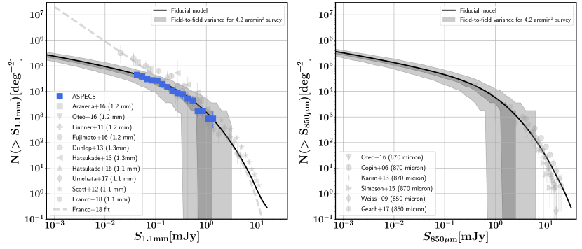
Figure 1: The 1.1 millimeter (left) and 850 $\mu$m (right) galaxy number counts. The black solid lines mark our predictions for the number counts when accounting for all the galaxies in the entire simulated lightcone. The dark– and light–gray shaded areas mark the one– and two–sigma scatter due to field–to–field variance, assuming a survey with the size of ASPECS (i.e., 4.2 arcmin²). The model predictions are compared to a literature compilation of number counts, where the dashed line corresponds to the Schechter fit presented by Franco et al. to their literature compilation. The blue points show the. number counts derived from ASPECS (González-López et al., 2020)

Figure 2: The predicted and observed 1.1 millimeter galaxy number counts in bins of redshift (top left), dust mass (top right), stellar mass (bottom left), and SFR (bottom right). The solid lines correspond to the model predictions, whereas the shaded areas show the ASPECS observations.

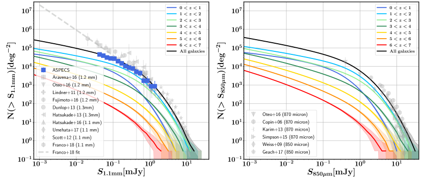
Figure 3: The 1.1 millimeter (left) and 850 $\mu$m (right) galaxy number counts. The black solid lines mark our predictions for the number counts when accounting for all the galaxies in the lightcone (as shown in Fig. 1). The coloured lines mark the number counts when selecting galaxies based on their redshift. The color shading corresponds to the two-sigma scatter when sampling over the intrinsic scatter of the empirical scaling relations. The model predictions are compared to a literature compilation of number counts as in Fig. 1. The 1.1 mm number counts are dominated by galaxies at $z=$1–2, with additional contributions from galaxies up to $z=3$ at the brightest fluxes and galaxies in the range $z=$0–1 at the faintest fluxes.

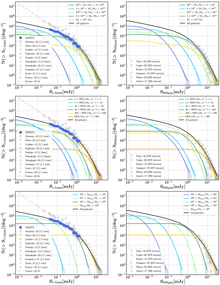
Figure 4: The 1.1 millimeter (left) and 850 $\mu$m (right) galaxy number counts of galaxies, broken up by different galaxy properties (integrated over all redshifts). The black solid lines mark our predictions for the number counts when accounting for all the galaxies in the lightcone (as shown in Fig. 1). The coloured lines mark the number counts when selecting galaxies based on their stellar mass (top row), SFR (middle row), and dust mass (bottom row). The color shading corresponds to the two-sigma scatter when sampling over the intrinsic scatter of the empirical scaling relations. The model predictions are compared to a literature compilation of number counts as in Fig. 1.

3 Results

In this Section we present our predictions for the 1.1 millimeter and 850 $\mu$m number counts of galaxies, specifically focusing on how they compare to current observations and which galaxies are responsible for the number counts at different flux densities. Throughout this paper we compare our model predictions to a set of observations taken from Coppin et al. (2006), Weiß et al. (2009), Lindner et al. (2011), Scott et al. (2012), Hatsukade et al. (2013), Karim et al. (2013), Simpson et al. (2015), Aravena et al. (2016), Dunlop et al. (2017), Fujimoto et al. (2016), Hatsukade et al. (2016), Oteo et al. (2016), Umehata et al. (2017), Geach et al. (2017), Franco et al. (2018), and González-López et al. (2020, the deepest survey at 1.2 millimeter over a contiguous area on the sky to date). This compilation includes observations based on single-dish instruments as well as with ALMA. These observations were carried out over a range of wavelengths, and scaled to 1.1 millimeter and 850 $\mu$m fluxes such that $S_{\rm 1.1mm}/S_{\rm 1.2mm}=1.36$, $S_{\rm 1.1mm}/S_{\rm 1.3mm}=1.79$, and $S_{\rm 870\mu\rm{m}}/S_{{\rm 850}\mu\rm{m}}=0.92$, assuming a dust emissivity index $\beta=1.5-2.0$ (e.g., Draine, 2011) and a temperature of 25–40 Kelvin (e.g.,Magdis et al. 2012; Schreiber et al. 2018). We first present the model number counts and how field–to–field variance affects the derived number counts. We then break up the number counts in bins of redshift, dust mass, stellar mass, and SFR. We finish by showing the redshift distribution of galaxies compared to observations.

3.1 The (sub-)mm number counts of galaxies and field-to-field variance

We present the 1.1 millimeter and 850 $\mu$m flux density number counts of galaxies in Figure 1 (black solid lines). The number counts predicted by the model are in good agreement with the ASPECS data, both at 1.1 millimeter and at 850 $\mu$m over the full flux density range where observations are available. We predict a flattening in the number counts of galaxies for flux densities below $\sim 0.3$ mJy at 1.1 millimeter, similar to the flattening found by González-López et al. (2020). We also find a flattening in the 850 $\mu$m number counts around a flux density of $\sim 1$ mJy. The predicted number counts lie below the observations by Fujimoto et al. (2016), who derived their number counts based on uncertain lensing models. Aravena et al. (2016) calculated their number counts based on a significantly smaller area and simpler analysis techniques. A more detailed description of the source of the discrepancy is given in (González-López et al., 2020).

Since one of the specific aims of this paper is to assess the origin of the flattening in the 1.1 mm number counts detected by González-López et al. (2020), we show the number counts derived for the entire simulated area, as well as the number counts derived for a simulated area corresponding to the ASPECS survey. To this aim we calculate the number counts in 100 randomly drawn sub-areas covering 4.2 arcmin² (the area covered by ASPECS) on the sky. The number counts of the full simulated volume are depicted as a black solid line, whereas the one- and two-sigma scatter when calculating the number counts in the areas corresponding to ASPECS are depicted as gray shaded regions. There are two noteworthy results with regards to cosmic variance. First of all, at flux densities fainter than 1 (3) mJy when focusing on 1.1 millimeter (850 $\mu$m) emission, the typical two-sigma scatter due to field-to-field variance is only a factor of 1.5 and the flattening in the number counts is always recovered. Second, due to the small area covered, sources brighter than 1 mJy (at 1.1 millimeter, 3 mJy at 850 $\mu$m) are typically missed by surveys targeting only 4.2 arcmin² on the sky (see also Figure 9).

3.2 Which galaxies are the main contributors to the number counts?

The depth of the ASPECS survey combined with the rich ancillary data available in the HUDF allowed González-López et al. (2020) to decompose the observed 1.2 millimeter number counts in bins of stellar mass, dust mass, SFR, and redshift. We compare our model predictions to these observations in Figure 2. We find decent agreement between the observations and model predictions when breaking up the number counts in bins of redshift, dust mass, and SFR. When breaking up the number counts in bins of stellar mass, we find that the contribution of galaxies with stellar masses between $10^{9}$ and $10^{10}\,\rm{M}_{\odot}$ is well reproduced. Our model predicts a contribution to the number counts below 0.5 mJy by galaxies with a stellar mass between $10^{10}$ and $10^{11}$ solar masses that is too large (up to a factor of two). The predicted contribution by galaxies with larger stellar masses in this flux density range is too small (up to a factor of three) compared to the observations. Tests have shown that when we change the stellar mass bins (e.g., from $10^{10.5}$ to $10^{11.5}\,\rm{M}_{\odot}$) the agreement between models and observations is much better. This suggests that the discrepancy is (at least partially) driven by uncertainties in the observed stellar masses that can easily be of the order 0.3 dex (Leja et al., 2019). We have furthermore not taken the effects of cosmic variance into account in this comparison, which can be non-negligible for the bins with highest stellar masses (Moster et al. 2011, since the ASPECS survey only covers an area of 4.2 squared arcsec in ALMA band 6). The good agreement between the model predictions is encouraging and opens up the opportunity to explore the model further to better understand which galaxies contribute to the number counts at different flux densities.

We show the number counts of galaxies in different redshift bins in Figure 3. Galaxies at $z>3$ make up for a small fraction of the total number counts at 1.1 millimeter and 850 $\mu$m. The number counts are made up by an equal contribution of galaxies in the redshift range $z=$2–3 and $z=$1–2 for flux densities brighter than $\sim$3 ($\sim 6$) mJy at 1.1 millimeter (850 $\mu$m). At lower flux densities, the largest contribution to the number counts comes from galaxies in the redshift bin $z=$1–2. Galaxies at $z<1$ hardly contribute to the number counts at flux densities larger than $\sim 0.1$ mJy at both wavelengths, whereas they contribute more importantly to the number counts at fainter fluxes (although still a factor of 2 less than galaxies at $z=$1–2). There is a clear flattening visible in the number counts of galaxies at all redshifts. The galaxy population that contributes most to the total (all redshifts) number counts at flux densities of 0.3 mJy at 1.1 millimeter (1 mJy at 850 $\mu$m, this corresponds to the flux density below which the total number counts rapidly flatten ) consists of galaxies with redshifts in the range $z=$1–2.

In Figure 4 we show the number counts of galaxies in bins of stellar mass. As the flux density increases the number counts are dominated by more massive galaxies. This is a natural consequence of an increase in dust mass and SFR of galaxies as a function of stellar mass. Galaxies with stellar masses around $5\times 10^{10}\,\rm{M}_{\odot}$ contribute most dominantly to the number counts at the flux density below which the number counts flatten (0.3 and 1 mJy at 1.1 millimeter and 850 $\mu$m, respectively).

We show the number counts of galaxies in bins of SFR in the middle row of Figure 4. Not surprisingly, we find that the number counts at the brightest flux densities probed by observations are dominated by the most actively star-forming galaxies (i.e., SFR $>100\leavevmode\nobreak\ \rm{M}_{\odot}\leavevmode\nobreak\ \rm{yr}^{-1}$). Interestingly, at $\sim$0.25 (0.6) mJy the 1.1 millimeter (850 $\mu$m) number counts are driven by an equal contribution from galaxies with a SFR in the bin between 10–50, 50–100, and 100–500 $\rm{M}_{\odot}\leavevmode\nobreak\ \rm{yr}^{-1}$. This pivoting point also roughly marks the location of the flattening in the number counts. At lower flux densities (but brighter than 0.05 and 0.1 mJy for the 1.1 millimeter and 850 $\mu$m number counts, respectively) the number densities are dominated by galaxies with a SFR $=$10–50 $\rm{M}_{\odot}\leavevmode\nobreak\ \rm{yr}^{-1}$. At even lower flux densities galaxies with SFRs between 1 and 5 $\rm{M}_{\odot}\,\rm{yr}^{-1}$ are predominantly responsible for the number counts. In the previous figures we noticed that as the flux density increases the number counts are dominated by more massive galaxies. Such a behavior is not seen for the SFR of galaxies. Some bins in SFR (e.g., 5–10 and 50–100 $\rm{M}_{\odot}\leavevmode\nobreak\ \rm{yr}^{-1}$) are never the dominant population of galaxies responsible for the observed total number counts. This is because the 1.1 millimeter and 850 $\mu$m fluxes of galaxies depend more strongly on dust mass than on SFR (see Equations 2 and 1).

The contribution by galaxies with different dust masses to the 1.1 millimeter and 850 $\mu$m number counts is also presented in Figure 4 (bottom row). Similar to the stellar mass, we find that as the flux density increases, the number counts are dominated by galaxies with increasing dust masses. We find that galaxies with dust masses in the range between $10^{8}$ and $10^{9}\,\rm{M}_{\odot}$ contribute most strongly to the number counts at 0.3 (1.0) mJy at 1.1 millimeter (850 $\mu$m), the flux density below which the number counts flatten.

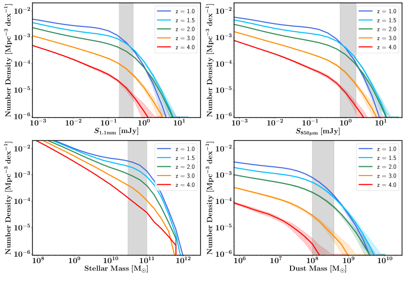
Figure 5: The 1.1 millimeter luminosity function (top left), the 850 $\mu$m luminosity function (top right), the stellar mass function (bottom left), and the dust mass function (bottom right) of galaxies at different redshifts. The color shading corresponds to the two-sigma scatter when sampling over the intrinsic scatter of the empirical scaling relations. The grey shaded band in each panel corresponds to the galaxies that contribute most dominantly to flux density at which the predicted flattening starts in the 1.1 millimeter and 850 $\mu$m number counts. The grey bands overlap with the knee of the respective mass/luminosity functions, suggesting that the flattening in number counts is a reflection of the 1.1 millimeter and 850 $\mu$m luminosity functions. We do not show the luminosity and mass functions at $z<1$ since the predicted flux densities at these redshifts are not reliable.

3.3 The flattening in number counts corresponds to the knee and shallow faint end slope of the dust continuum luminosity functions

In the previous subsection we have seen that our model and the observations suggest that galaxies at $z=$1–2 contribute most to the flux densities at which the 1.1 millimeter and 850 $\mu$m number counts flatten (Figure 3). We have furthermore seen that the galaxies responsible for the flattening have stellar masses around $5\times 10^{10}\leavevmode\nobreak\ \rm{M}_{\odot}$, dust masses between $10^{8}$ and $10^{9}\leavevmode\nobreak\ \rm{M}_{\odot}$, and SFRs in the range between 10 and 500 $M_{\sun}$ yr^-1. At $z=$1–2, a stellar mass of $5\times 10^{10}\leavevmode\nobreak\ \rm{M}_{\odot}$ roughly corresponds to the stellar mass at the knee of the stellar mass function at these redshifts (e.g., Tomczak et al., 2014). This suggests that the flattening in the number counts is driven by the shape of the 1.1 millimeter and 850 $\mu$m luminosity function at $z=$1–2 and that the flattening may actually simply reflect observations probing galaxies below the knee of this function.

To test our hypothesis we switch from number counts (projected densities on the sky) to volume densities. In Figure 5 we show the luminosity function (number of sources per volume element) predicted from our model as a function of redshift (cosmic time). We also show the stellar mass function and dust mass functions. We highlight the flux density and stellar (dust) mass regime at which the flattening occurs with a vertical grey band. Indeed, the knee of the luminosity function at $z=1.5$ (in the middle of the redshift range $z=$1–2) corresponds to the flux densities at which the flattening in the number counts occurs. Similarly, the stellar and dust mass at which the flattening occurs in the number counts corresponds to the knee of the respective mass functions at $z=1.5$. We furthermore find that the faint–end slope of the dust continuum luminosity functions (and dust mass function) is significantly shallower than the low–mass slope of the stellar mass function (almost flat at $z<2$; compare the top two panels to the bottom left panel). This is driven by the strong dependence of the gas–phase metallicity on stellar mass and the strong dependence of the dust-to-gas ratio on the gas-phase metallicity. Because of this shallow slope in the dust continuum luminosity function, integrating to fainter flux densities results in only a modest increase in detected sources, as will be discussed in Sec. 4. The flattening in the number counts thus corresponds to probing galaxies below the knee of the luminosity function.

Our model assumes that a set of empirical relations can be used to describe the entire population of galaxies from low to high redshifts. It is therefore worthwhile to explore if our finding that the flattening in the number counts is caused by the shape of the dust continuum luminosity function is robust against changes in the assumed empirical relations. In Appendix A of this work we adopt a variety of different assumptions, including different recipes to assign gas masses to galaxies, different mass-metallicity relations, a different assumption for the amount of star formation that is dust obscured, and different assumptions for the dust–to–gas ratio of galaxies. Every empirical relation used in the model has an error associated to it. To better understand how the error in these components affects the number counts we run the model 100 times, sampling over the intrinsic error for each empirical relation. The different assumptions change the normalization of the number counts by up to a factor of two. It furthermore slightly changes the shape of the cumulative number counts. Nevertheless, for none of the explored scenarios does the flattening in the number counts disappear. In other words, this flattening is not driven by changes in the assumptions on how we derive the dust-to-gas ratio of galaxies, their gas mass, the fraction of obscured star-formation, their metallicity, or the uncertainties in the individual model components. This strengthens our conclusion that the flattening in the number counts is simply caused by the distribution of the underlying galaxy population, i.e., probing galaxies below the knee of the dust continuum luminosity functions/mass functions.

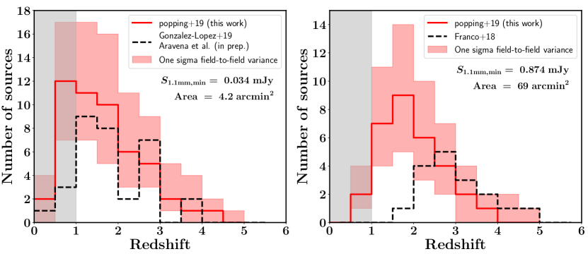
Figure 6: A comparison between the predicted and observed redshift distribution of galaxies observed at 1.1 millimeter. To account for field–to–field variance, we calculate the number counts 1000 times over a random portion of the entire modeled lightcone covering the same area as the observations, imposing the same survey depth (as outlined in the individual panels). The solid line corresponds to the median redshift distribution, whereas the shaded region corresponds to the one-sigma scatter. Model predictions are compared to the observations by González-López et al. (2020, left) (and Aravena et al in prep.) and Franco et al. (2018, right). The gray shaded area (at $z<1$) marks the regime where the model predictions can not be fully trusted because the negative k–correction does not apply anymore at those redshifts.

3.4 Redshift distribution

Current (sub-)millimeter surveys with ALMA have predominantly detected galaxies at redshifts $z<3.5$ (see for example Figure 18 in Franco et al. 2018 and other figures in Aravena et al. 2016 and Bouwens et al. 2016 and González-López et al. 2020). Even though ALMA has pushed the detection limit of galaxies to flux densities below 0.1 mJy, the fraction of galaxies at redshifts larger than 3.5 still remains very low. This is driven by the dominant contribution of galaxies at $z=1-3$ to the number counts (Fig. 3).

To quantify the agreement between the redshift distribution of (sub-)mm detections predicted by our model and the current observations, we present a comparison between the two in Figure 6. For this comparison, we adopt the same field–of–view and sensitivity cutoff as the observations. We compare our predictions to observational results by Franco et al. (2018) and González-López et al. (2020). These works probe the 1.1 millimeter number counts over an area of 69 arcmin² (Franco et al., 2018) down to 0.874 mJy and an area of 4.2 arcmin² down to 0.034 mJy (González-López et al., 2020). To account for field–to–field variance, we calculate the number counts 1000 times over a random portion of the entire modeled lightcone covering the same area as the observations (similar to Figure 1). We show the mean and one-sigma distribution of the predicted number counts. The predicted redshift distribution at $z<1$ can not fully be trusted, as the negative k–correction implied by our model does not apply at these redshifts.

Overall we find that the observed redshift distributions from González-López et al. (2020) typically all fall within the one-sigma scatter of the model predictions. This suggests that, at least at $z<3$, the model not only successfully reproduces the cumulative number counts of galaxies, but also the redshifts of the sources that are responsible for these number counts. The low-number statistics of detections at $z>4$ makes it hard to further quantify the success of the presented model. Possibly most surprising is the lack of sources detected by Franco et al. (2018) at $z<2$ compared to our model predictions. We additionally find that at $\sim 1$ mJy, our model predicts number counts higher than derived by Franco et al. (2018). Given the success of our model in reproducing the number counts by González-López et al. (2020), the apparent mismatch with Franco et al. may suggest a tension between the model predictions and observations for the brightest millimeter sources, but we note that not all sources in the Franco et al. 2018 sample have a spectroscopic redshift. Furthermore, a prior based selection of the data presented in Franco et al. suggested that additional sources may have been missed in the blind selection, which may change the redshfit distribution (Franco et al. in prep). Lastly, it has to be noted that the observations still fall within the two–sigma range of the model predictions. Our model predicts a higher median redshift for a survey similar to Franco et al. (2018) than González-López et al. (2020) (although the median redshift predicted for a survey with the Franco et al. specifics is different from what was observed). This is in agreement with previous findings that the survey depth can significantly alter the redshift distribution with shallower surveys yielding higher mean redshifts (Béthermin et al., 2015).

4 Discussion

4.1 Observational consequences

We have presented a new data driven model for the cumulative number counts and redshift distribution of (sub–)millimeter detections of galaxies. This model successfully reproduces current observations (the cumulative number counts, number counts in bins of different galaxy properties, and redshift distribution functions), including the flattening in the 1.1 millimeter number counts observed by González-López et al. (2020). There is a simple origin for this flattening, namely the shape of the underlying luminosity function of galaxies at 1.1 millimeter in the redshift range between $z=1$ and $z=2$ (probing the knee and shallow faint end slope). We have furthermore demonstrated that this conclusion is robust against field-to-field variance and the assumptions made in the presented model. The predicted (and observed) flattening in the number counts has clear consequences for future continuum surveys with ALMA. A survey at 1.1 millimeter deeper than 0.1 mJy will not significantly increase the number of detected sources per square degree. A similar flattening is to be expected for the 850 $\mu$m number counts below 1 mJy, a flux density regime only probed by Oteo et al. (2016) so far. Given our predictions, a future deep survey at 850 $\mu$m will detect fewer sources than naively have been expected when extending a simple fit to the current 850 $\mu$m number count observations.

We can further quantify this by looking into the expected results of hypothetical surveys. In Figure 8 we show the expected number of sources for a survey covering a given area to a given depth. We furthermore show how many hours per pointing it takes to reach that depth (adopting a signal-to-noise ratio of three and assuming standard ALMA assumptions in the respective bands with 50 antennas), and how many pointings are needed to cover the targeted area adopting Nyquist sampling. On the top two panels, we also plot contours that mark a fixed number of expected detections. As expected, an increase in area and an increase in depth both result in a larger number of detected galaxies. Below 0.1 mJy (for 1.1 millimeter, 0.3 mJy for 850 $\mu$m) the contours of constant number of sources are almost horizontal (i.e., scale less strongly with sensitivity than with area). An increase in the depth from 0.1 to 0.01 mJy only results in an increase of a factor of $\sim$3 in the detected number of sources. An increase of the area with an order of magnitude naturally results in an increase of a factor 10 in the detected number of sources. This suggest that if the goal of the survey is to detect large number of sources for better statistics, an increase in area is more effective than an increase in survey depth once one has reached a depth of $\sim$0.1 mJy at 1.1 millimeter ($\sim$ 0.3 mJy at 850 $\mu$m).

In the bottom two panels of Figure 8, we show contours of fixed total on source time necessary to perform such a survey. This clearly shows that to detect a large number of sources for proper statistics a wide survey is more time efficient than a deep survey. Figure 8 also shows that although galaxies are intrinsically brighter at 850 $\mu$m, a survey at 1.1 mm is actually more time efficient. Because the primary beam of ALMA at 1.1 millimeter is larger than at 850 $\mu$m, within a fixed time a survey at 1.1 millimeter can detect fainter sources over a given area than a survey at 850 $\mu$m (as the time is distributed over fewer pointings and thus a fainter sensitivity limit can be reached). The number of expected detected sources per square arc minute is roughly the same between a survey at 850 $\mu$m and 1.1 millimeter for a fixed on source observing time.

In Figure 9 we plot the redshift distribution of galaxies per arcmin² for surveys reaching different depths. We explore the redshift distribution when accounting for galaxies with flux densities brighter than 0.01, 0.1, and 1 mJy, respectively. We mark the redshift range $z<1$ with a grey vertical band, as the negative k–correction assumed in our model does not apply for this redshift range.

As the depth of the survey increases, the number of galaxies per arcmin² increases at every redshift. The number of galaxies detected per arcmin² is systematically higher at 850 $\mu$m than at 1.1 mm by a factor of three for a survey down to 1 mJy and a factor of 1.5 for a survey down to 0.1 mJy and 0.01 mJy. This is the natural consequence of the shape of the (sub-)millimeter SED of galaxies, i.e., lower flux densities at longer wavelengths. Interestingly enough, the median redshift of the redshift distributions is very similar for all three survey depths (around $z=1.5$, although note that the uncertain $z<1$ redshift range at which our model may over predict the brightness of sources is included). This seems in tension with observational results (e.g., the higher median redshift of Franco et al. (2018) than González-López et al. (2020)), similar to what we saw in Figure 6.

At 1.1 millimeter, a survey reaching a depth of 0.1 mJy will detect approximately an order of magnitude more sources at $1<z<4$ (up to a factor of 30 at $z\sim 5$) than a survey reaching a depth of 1 mJy. An increase in sensitivity down to 0.01 mJy yields another factor of $\sim 3$ increase in the number of galaxies per arcmin² at $z>1$. At 850 $\mu$m a survey with a depth of 0.1 mJy will detect a factor of 8–10 more galaxies than a survey with a depth of 1 mJy at $z>1$. An additional factor of two can be gained by integrating down to a sensitivity of 0.01 mJy. This again emphasises that below flux densities of 0.1 (0.3) mJy at 1.1 millimeter (850 $\mu$m), the number of expected sources only moderately increases with increasing survey depth. At those densities a survey is probing the faint end slope of the dust continuum luminosity function (top two panels Figure 5).

Summarising, to significantly increase the number of sources with dust continuum counterparts, a wide survey at 1.1 millimeter at flux density of $\sim 0.1$ mJy is most cost efficient. A gain of only a factor 10 in the number of detected sources compared to the results of González-López et al. (2020) could already heavily increase the constraining power for models. Not only will it improve the high-redshift statistics (currently poorly understood), it is also a better approach to obtain dust-continuum counterparts of as many objects as possible that are already detected through optical and near-infrared surveys in common legacy fields. This will allow a more detailed break-down of number counts over different galaxy properties as suggested in this work (e.g., as a function of stellar mass and SFR) and a dust-continuum based gas and dust mass estimate for increasingly large number of galaxies (e.g., Aravena et al., 2016; Scoville et al., 2016; Magnelli et al., 2019). The exact survey strategy will ultimately depend on the scientific requirements.

4.2 What a successful empirical model says about galaxy scaling relations

Our semi-empirical model combines a data-driven model for the stellar mass and SFR population of galaxies over cosmic time (Behroozi et al., 2019) with a number of empirical relations to connect the SFR and stellar mass of galaxies to their dust continuum emission. It is comforting to realize that this combination correctly reproduces the observed 1.1 millimeter and 850 $\mu$m number counts. What this teaches us is that the adopted scaling relations all seem to hold at least over the redshift regime $z=$0–2 (i.e., the redshift range that most dominantly contributes to the number counts). This is especially relevant for the adopted relation between dust–to–gas ratio and gas–phase metallicity and the scaling between dust mass, SFR, and 1.1 millimeter and 850 $\mu$m dust continuum flux density, as these relations have only been observationally probed in this redshift range for a limited number of massive galaxies (e.g., Aravena et al., 2016; Dunlop et al., 2017; Miettinen et al., 2017; Aravena et al., 2019; Magnelli et al., 2019). We have indeed seen (see Appendix A) that a different choice for the dust–to–gas ratio and mass–metallicity relation results in poorer agreement between the model predictions and observations. It is furthermore encouraging to see that that the Hayward et al. fitting relations for the dust continuum emission of galaxies result in good agreement with observed number counts, even though these fitting relations were derived for galaxies with flux densities brighter than 0.5 mJy.

Except for the redshift range between $z=1-2$, the constraining power of number counts for our understanding of galaxy physics over cosmic time is rather limited. The fact that our model successfully reproduces the redshift distribution of 1.1 millimeter detections up to $z=4$ (within one sigma) is encouraging, but the low number statistics in the $z=$2–4 redshift range does not allow us to make further claims on the validity of the adopted scaling relations in that redshift regime. It is even harder to make any claims about the physics at higher redshifts. For example, the contribution of galaxies at $z>4$ to the number counts is very limited and an order of magnitude increase or decrease in the number of dusty galaxies at $z>4$ would not change the cumulative number counts significantly. This suggests that we have almost exhausted what can be learned about galaxy physics from cumulative number counts. It is therefore important that future observations start to probe the luminosity function of galaxies at discrete redshifts (and possibly the dust mass function), start connecting the dust continuum measurement to other galaxy properties, and furthermore aim at resolving the interiors of galaxies at sub-mm wavelengths. This requires among others complete spectroscopic redshift samples for sizeable numbers of (sub-mm) galaxies. Besides confirming our theoretical hypothesis about the flattening caused by the knee of the mass/luminosity functions at $z=$1–2 and the shallow faint end slope, such an effort will provide stringent constraints currently missing for theoretical models that started to include the detailed tracking of dust formation and destruction over cosmic time (McKinnon et al., 2017; Popping et al., 2017; Hou et al., 2019; Davé et al., 2019). These include constraints on the dust mass function, cosmic density of dust, but also the connection between stellar mass and SFR and dust properties. An approach to observationally probe the luminosity function would be to cross-correlate the securely detected dust continuum sources with information from spectroscopic surveys of the UDF for example with MUSE (Inami et al., 2017; Boogaard et al., 2019) or based on ALMA spectral information (González-López et al., 2019).

4.3 A top-heavy initial mass function?

Previous theoretical works have suggested that a top–heavy IMF in starburst environments is necessary to reproduce the number count of bright galaxies, while simultaneously reproducing the optical and near-infrared properties of galaxies (e.g., Baugh et al., 2005; Lacey et al., 2016). Recent observations of active star-forming regions (analogues of high-redshift starbursts) in our Galaxy and the Large Magellanic Cloud (Motte et al., 2018; Schneider et al., 2018) have suggested that the newly formed stars in these regions indeed have a top-heavy IMF compared to a Chabrier IMF. Zhang et al. (2018) looked at the abundance ratio of isotopologues (an index of the IMF, Romano et al. 2017) in $z=2-3$ dust-enshrouded starbursts and concluded that these galaxies have an IMF more top-heavy than a Chabrier IMF.

We find that we can reproduce the number counts of galaxies at 1.1 millimeter and 850 $\mu$m (up to a few tens of mJy at 850 $\mu$m) under the assumption of a uniform Chabrier (2003) IMF. This is in line with other recent theoretical efforts that suggest that the number counts of sub-millimeter bright galaxies can be reproduced without invoking a top-heavy IMF (e.g., Safarzadeh et al., 2017; Lagos et al., 2019). This does not necessarily mean that starburst environments can not form stars following a different IMF than Chabrier. It suggests that changes in the IMF in order to match sub-mm number counts are degenerate with other ingredients and predictions of galaxy formation models such as the treatment of dust and dust emission and/or the SF properties of galaxies. These degeneracies should be explored with care.

4.4 Comparison to earlier work

There have been multiple theoretical efforts in the literature (some of them from first principles, others adopting a semi-empirical approach similar to our model) that model the (sub-)mm number counts of galaxies. Pre-ALMA, the focus of these comparisons was on the sub-millimeter galaxies that are orders of magnitude brighter than the sources discussed in this work. Only after ALMA started operations did these comparisons start to include sources with flux densities below 1 mJy.

Somerville et al. (2012) presented predictions for the 850 $\mu$m number counts down to 0.01 mJy, based on a semi-analytic model of galaxy formation (Somerville et al., 2008). This model predicts a sharp drop in the differential number counts of galaxies for flux densities below 0.1 mJy. The model does not succeed in reproducing the observational constraints that were available at that time.

Cowley et al. (2017) use a different semi-analytic model to study 850 $\mu$m number counts of galaxies. The authors reproduce the observations and predict a flattening in the number counts, but do not explore what causes this flattening. The authors specifically focus on the effect of field-to-field variance on observed number counts and similar to us find that survey design influences how well the underlying ‘real’ number count distribution of galaxies is recovered.

Lacey et al. (2016) provides predictions for the 850 $\mu$m number counts using the same semi-analytic model as Cowley et al. (2017). The authors specifically explore how different prescriptions for the baryonic physics in galaxies affect the number counts, but found all explored prescriptions predict a flattening in the number counts. This strengthens our conclusion that the flattening is caused by the underlying galaxy population. The authors furthermore explore the redshift distribution of sub-mm detected galaxies, but focus on surveys with a depth of 5 mJy. In order to reproduce the observed number counts (especially for the brightest flux densities) Lacey et al. (2016) adopt a top-heavy IMF during starburst events (see also Baugh et al. 2005). Our work on the other hand suggests that the number counts can be reproduced by a simple semi-empirical model that does not need to make any changes to the initial mass function of the stars.

Safarzadeh et al. (2017) present predictions for the 850 $\mu$m number counts of galaxies based on a semi-analytic model (Lu et al., 2011, 2014). In this work the authors calculate the 850 $\mu$m flux of galaxies by coupling the SAM output to the fitting functions presented in Hayward et al. (2013b). The presented predictions agree fairly well with the observations that were available at that time (although they seem to predict higher number densities than found by Aravena et al. (2016) after rescaling to 850 $\mu$m). The model predictions include a flattening of the cumulative number counts below 850 $\mu$m flux densities $\sim 1$ mJy, in rough agreement with our predictions. The main result of Safarzadeh et al. (2017) is that the observed 850 $\mu$m number counts can be reproduced by the models without invoking the need of a top-heavy IMF, in line with our findings. This also agrees with the findings using a different semi-analytic model by Lagos et al. (2019), who reach a similar conclusion by predicting the 850 $\mu$m flux density directly from the star-formation history of the galaxies with a physical model for attenuation.

Hayward et al. (2013b) couples a semi-empirical model with the fitting functions from Hayward et al. (2011) to model the number counts at 1.1 millimeter at flux densities brighter than 0.5 mJy. The model reproduced the available constraints at that time, but did not look at faint enough galaxies to probe the existence of the flattening in the 1.1 millimeter number counts. The authors furthermore present the redshift distribution function for a survey at 1.1 millimeter with a flux density sensitivity of 1.5 mJy and find a median redshift of $z=3$, with a quick drop at $z>4$. This median redshift is higher than predicted by our model. The origin of this difference may lie in the adopted approach to estimate the dust mass of galaxies. Hayward et al. (2013b) adopt a fixed dust–to–metal ratio, a different mass–metallicity relation, and a different approach to estimate the gas mass of galaxies. As demonstrated in the Appendix of this paper (see Figure 7), these different approaches result in changes in the normalization of the number counts and small changes in their shape. Especially given the difference between the Zahid et al. (2013) and Maiolino et al. (2008) mass–metallicity relation, it is not surprising that this leads to a different redshift distribution.

Similar to the work presented in this paper, Hayward et al. (2013a) coupled the fitting functions from Hayward et al. (2011) to the sub-halo abundance matching model presented in Behroozi et al. (2013a). Hayward et al. were particularly interested in the effects of blending (i.e., spatially and physically unassociated galaxies blending within one beam) on the derived 850 $\mu$m number counts of single-dish surveys and found that, indeed, for single dish surveys blending contributes significantly to the number counts at flux densities brighter than 2 mJy (the exact contribution of blending to the bright end of the number counts depends on the adopted beam size). In this work we are mostly comparing our model predictions to observations that probe fainter regimes (fainter than 2 mJy at 850 $\mu$m) where blending is less of an issue and/or based on ALMA results, for which the beam size is sufficiently small to easily separate the individual sources.

Béthermin et al. (2017, see also ) developed a semi-empirical model for the number counts of galaxies. This model is conceptually similar to the work presented here, but also accounts for the effect of lensing on the number counts of galaxies. The authors find a flattening in the 1.2 millimeter number counts at flux densities below 0.1 mJy, although not as strong as we find and suggested by observations. The authors furthermore explore the redshift distribution of galaxies, exploring a scenario with a survey depth of 4 mJy at 850 $\mu$m and 1.5 mJy at 1.2 millimeter (see also Béthermin et al. 2015). Béthermin et al. (2017) find that for the latter scenario the redshift distribution peaks at around $z=$2–3, slightly higher than our findings. The authors do not aim to explore what the properties are of the galaxies that contribute to the number counts at different flux densities.

Casey et al. (2018) also presented a model for the (among others) 1.1 millimeter and 850 $\mu$m number counts. Casey et al. explore a number of star-formation history scenarios (especially focusing on the fraction of dust-obscured SF at $z>4$) and investigate how these changes in the star-formation histories manifest themselves in the (sub–)millimeter number counts. The authors do not focus on flux densities faint enough to discuss their theoretical predictions for a flattening in the number counts.

5 Conclusions

In this paper we presented a semi-empirical model for the number counts of galaxies at 1.1 millimeter and 850 $\mu$m. This model is based upon the UniverseMachine (Behroozi et al. 2019, a model that predicts the stellar mass and SFR distribution of galaxies over cosmic time) with theoretical and empirical relations that predict the dust emission of galaxies as a function of their SFR and dust mass. This model can explain the observations at flux levels that were not reachable pre–ALMA. We summarise our main results below.

• The predictions by our fiducial model are in good agreement with the observed cumulative number counts and number counts in bins of different galaxy properties. The model reproduces the flattening observed in the 1.1 millimeter number counts of recent deep surveys with ALMA. A similar flattening is predicted for 850 $\mu$m number counts below 1 mJy.

• We demonstrate that the flattening in the 1.1 millimeter number counts reflects the shape of the underlying galaxy population at $z=$1–2, i.e., the observations are probing the knee and the shallow faint end slope of the 1.1 millimeter luminosity function.

• The galaxies at the ‘knee’ of the 1.1 millimeter number counts have redshifts between $z=1$ and $z=2$, stellar masses around $5\times 10^{10}\rm{M}_{\odot}$ and dust masses of the order $10^{8}\leavevmode\nobreak\ \rm{M}_{\odot}$.

• The observed ASPECS redshift distribution of 1.1 millimeter ALMA detections is in agreement with the model predictions after we account for field–to–field variance.

• Future dust continuum surveys at 1.1 millimeter and 850 $\mu$m surveys that aim to detect large numbers of sources through their dust emission should cover large areas on the sky once below a flux density of $\sim$0.1 mJy (at 1.1 millimeter, $\sim$ 0.3 mJy at 850 $\mu$m), rather than integrating to faint flux densities over small portions on the sky.

• Our model successfully reproduces the number counts of galaxies without the need to adopt an IMF different from Chabrier (2003). This is in contrast with theoretical models suggesting that a top–heavy IMF is responsible for the observed number counts of bright millimeter galaxies.

• The success of our model to reproduce the number counts of galaxies suggest that the adopted empirical relations in our fiducial model (to estimate the gas mass, the gas-phase metallicity, obscured fraction of star formation, dust mass, and dust continuum flux of galaxies) are valid up to $z=2$. Different choices for the empirical relations lead to poorer agreement with the observations.

The success of our model to describe the number counts of galaxies at 1.1 millimeter and which galaxies are responsible for these number counts also means that we have exhausted the amount of information about galaxy physics that can be extracted from dust continuum number counts. Mainly because the number counts are biased towards a narrow redshift range from redshift one to two. To further our knowledge about galaxy physics from continuum observations, future observational efforts should focus on the dust continuum properties in discrete redshift bins (e.g., dust continuum luminosity function), as a function of other galaxy properties, and on spatially resolved, multi–band dust continuum properties of galaxies and their connection to the resolved stellar and gas properties of galaxies.

Appendix A Is the flattening in the number counts robust against the assumptions made in the semi-empirical model

In the main body of this paper we have connected the predictions from the UniverseMachine to a number of empirical relations to estimate the sub-mm flux density of galaxies. In this Appendix we explore how robust our results are against the exact choice in these empirical relations. We replace the empirical relations in our fiducial model by other relations/assumptions proposed in the literature and show the resulting predicted number counts in Figure 7.

Gas masses estimated following Saintonge et al. (2013)

We have adopted the methodology presented in Popping et al. (2015a) to estimate the gas mass (atomic plus molecular) of galaxies. An alternative option is the fit for the H₂ mass of galaxies as a function of stellar mass, SFR, and redshift given in (Saintonge et al. 2013, note that this prescription does not include a contribution by Hi to the total gas mass). We find that the number counts are systematically a factor 1.5–2 below the predictions of our fiducial model.

Fixed dust–to–metal ratio of 0.4

Theoretical models typically make the assumption that the dust-to-metal ratio of the ISM equals 0.4. When adopting the same value (thus not scaling the dust-to-metal ratio of the ISM as a function of the gas-phase metallicity) the predicted number counts are a factor of 1.5–2 above the predictions by our fiducial model. Although the overall normalization of the number counts changes, the flattening does not disappear.

Mass-metallicity relation from Maiolino et al. (2008)

An alternative fit of the gas-phase metallicity of galaxies as a function of their stellar mass and redshift in the redshift range from $z=0$ to $z=3.5$ was presented in Maiolino et al. (2008). We adopted the Zahid et al. (2013) relation for our fiducial model as this is based on a more robust sample of galaxies with a coherent metallicity calibration. The number counts predicted when adopting the Maiolino et al. (2008) mass-metallicity relation are a factor $\sim 1.5$ below the predictions by our fiducial model.

All star-formation is obscured

We adopted the fit presented in Whitaker et al. (2017) to estimate the obscured fraction of SF. An extreme alternative is to assume that all SF happens in dust environments and $f_{\rm obscured}=1$. We find that the resulting number counts are essentially the same as predicted by our fiducial model, expect for the faintest flux densities.

Summarising, we find that the exact choice for the individual components of our model change the normalization of the number counts, but not the presence of a flattening. This confirms that the flattening seen in the data is indeed a result of the underlying galaxy population and not due to the adopted approach to assign sub-mm luminosities to galaxies.

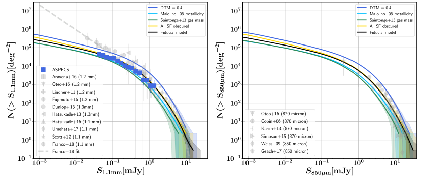
Figure 7: The observed and predicted 1.1 millimeter and 850 $\mu$m galaxy number counts. The black solid line marks the fiducial model discussed in this paper. The coloured lines mark the number counts when replacing individual components of the model by different empirical relations/assumptions discussed in the Appendix. The shaded region marks the one-sigma variance of the 100 random realizations when sampling over the error of the individual components of the model. There are some changes in the normalization of the number counts when varying individual components of the model within a facor of $<$2, but overall the shape of the number counts is robust against the changes applied to the model.

Appendix B A hypothetical survey

In Figures 8 and 9 we show predicted number of observed galaxies and their redshift distribution, respectively, of hypothetical future surveys (with ALMA). These are discussed in detail in Section 4.1

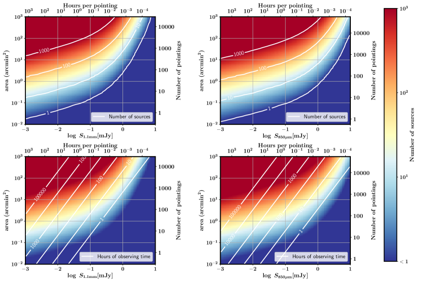
Figure 8: The expected number of sources for a hypothetical survey at 1.1 millimeter (left column) and 850 $\mu$m (right column), as a function of the survey depth and covered area, as well as the number of hours per pointing it takes to reach this depth (at a signal-to-noise ratio of 3) and the number of pointings necessary to cover the area assuming Nyquist sampling (all assuming standard ALMA assumptions for 50 antenna’s). In the top row, contours depict lines of a fixed number of expected sources. In the bottom row, contours depict a fixed total on source observing time. Below flux densities of 0.1 (0.3 mJy) a wide survey at 1.1 millimeter (850 $\mu$m) is more (cost-)efficient to increase the number of detected source than a deep pointed survey.

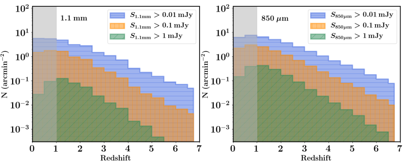
Figure 9: The redshift distribution of galaxies as a function of their 1.1 millimeter (left) and 850 $\mu$m (right) flux density. A different survey depth results in preferably detecting galaxies at different redshift. To efficiently detect galaxies, a shallow but wide survey is more time efficient that a narrow but deeper survey. The gray shaded area (at $z<1$) marks the regime where the model predictions can not be fully trusted because the negative k–correction does not apply anymore at those redshifts.

References

- Aravena et al. (2016) Aravena, M., Decarli, R., Walter, F., et al. 2016, ApJ, 833, 68
- Aravena et al. (2019) Aravena, M., Decarli, R., Gónzalez-López, J., et al. 2019, ApJ, 882, 136
- Baugh et al. (2005) Baugh, C. M., Lacey, C. G., Frenk, C. S., et al. 2005, MNRAS, 356, 1191
- Behroozi et al. (2019) Behroozi, P., Wechsler, R. H., Hearin, A. P., & Conroy, C. 2019, MNRAS, 488, 3143
- Behroozi et al. (2013a) Behroozi, P. S., Wechsler, R. H., & Conroy, C. 2013a, ApJ, 770, 57
- Behroozi et al. (2013b) Behroozi, P. S., Wechsler, R. H., & Wu, H.-Y. 2013b, ApJ, 762, 109
- Behroozi et al. (2013c) Behroozi, P. S., Wechsler, R. H., Wu, H.-Y., et al. 2013c, ApJ, 763, 18
- Béthermin et al. (2015) Béthermin, M., De Breuck, C., Sargent, M., & Daddi, E. 2015, A&A, 576, L9
- Béthermin et al. (2012) Béthermin, M., Daddi, E., Magdis, G., et al. 2012, ApJ, 757, L23
- Béthermin et al. (2017) Béthermin, M., Wu, H.-Y., Lagache, G., et al. 2017, A&A, 607, A89
- Bigiel et al. (2008) Bigiel, F., Leroy, A., Walter, F., et al. 2008, AJ, 136, 2846
- Blitz & Rosolowsky (2006) Blitz, L., & Rosolowsky, E. 2006, ApJ, 650, 933
- Boogaard et al. (2019) Boogaard, L. A., Decarli, R., González-López, J., et al. 2019, ApJ, 882, 140
- Bouwens et al. (2016) Bouwens, R. J., Aravena, M., Decarli, R., et al. 2016, ApJ, 833, 72
- Carniani et al. (2015) Carniani, S., Maiolino, R., De Zotti, G., et al. 2015, A&A, 584, A78
- Casey et al. (2014) Casey, C. M., Narayanan, D., & Cooray, A. 2014, Phys. Rep., 541, 45
- Casey et al. (2018) Casey, C. M., Zavala, J. A., Spilker, J., et al. 2018, ApJ, 862, 77
- Chabrier (2003) Chabrier, G. 2003, PASP, 115, 763
- Coppin et al. (2006) Coppin, K., Chapin, E. L., Mortier, A. M. J., et al. 2006, MNRAS, 372, 1621
- Cowley et al. (2017) Cowley, W. I., Béthermin, M., Lagos, C. d. P., et al. 2017, MNRAS, 467, 1231
- Cowley et al. (2015) Cowley, W. I., Lacey, C. G., Baugh, C. M., & Cole, S. 2015, MNRAS, 446, 1784
- da Cunha et al. (2013) da Cunha, E., Groves, B., Walter, F., et al. 2013, ApJ, 766, 13
- Davé et al. (2019) Davé, R., Anglés-Alcázar, D., Narayanan, D., et al. 2019, MNRAS, 486, 2827
- De Vis et al. (2019) De Vis, P., Jones, A., Viaene, S., et al. 2019, A&A, 623, A5
- Decarli et al. (2019) Decarli, R., Walter, F., Gónzalez-López, J., et al. 2019, ApJ, 882, 138
- Draine (2011) Draine, B. T. 2011, Physics of the Interstellar and Intergalactic Medium
- Dunlop et al. (2017) Dunlop, J. S., McLure, R. J., Biggs, A. D., et al. 2017, MNRAS, 466, 861
- Eales et al. (2000) Eales, S., Lilly, S., Webb, T., et al. 2000, AJ, 120, 2244
- Feldmann (2015) Feldmann, R. 2015, MNRAS, 449, 3274
- Fixsen et al. (1998) Fixsen, D. J., Dwek, E., Mather, J. C., Bennett, C. L., & Shafer, R. A. 1998, ApJ, 508, 123
- Fontanot et al. (2009) Fontanot, F., Somerville, R. S., Silva, L., Monaco, P., & Skibba, R. 2009, MNRAS, 392, 553
- Franco et al. (2018) Franco, M., Elbaz, D., Béthermin, M., et al. 2018, A&A, 620, A152
- Fujimoto et al. (2016) Fujimoto, S., Ouchi, M., Ono, Y., et al. 2016, ApJS, 222, 1
- Geach et al. (2017) Geach, J. E., Dunlop, J. S., Halpern, M., et al. 2017, MNRAS, 465, 1789
- González-López et al. (2019) González-López, J., Decarli, R., Pavesi, R., et al. 2019, ApJ, 882, 139